Motor Control With Arduino MathWorks

7/17/2019 Motor Control With Arduino MathWorks

http://slidepdf.com/reader/full/motor-control-with-arduino-mathworks 1/14

Motor Control with Arduino: A Case Study in Data-Driven Modelling and Control Design

By Pravallika Vinnakota, MathWorks

Tuning a controller on a physical prototype or plant hardware can lead to unsafe operating conditions

and damage the hardware. A more reliable approach is to build a plant model and simulate it to verify

the controller at different operating conditions so as to run what-if scenarios without risk.

When first-principles modelling is not feasible, an alternative is to develop models from input-output

measurements of the plant. A low-order, linear model might be sufficient for designing a basic

controller. Detailed analysis and design of a higher-performance controller requires a higher-fidelity

and possibly nonlinear model.

Using a simple control system for a DC motor as an example, this article shows how to identify a plant

model from input-output data, use the identified model to design a controller, and implement it. Theworkflow includes the following steps: acquiring data, identifying linear and nonlinear plant models,

designing and simulating feedback controllers, and implementing these controllers on an embedded

microprocessor for real-time testing.

The DC Motor: Control Design Goals

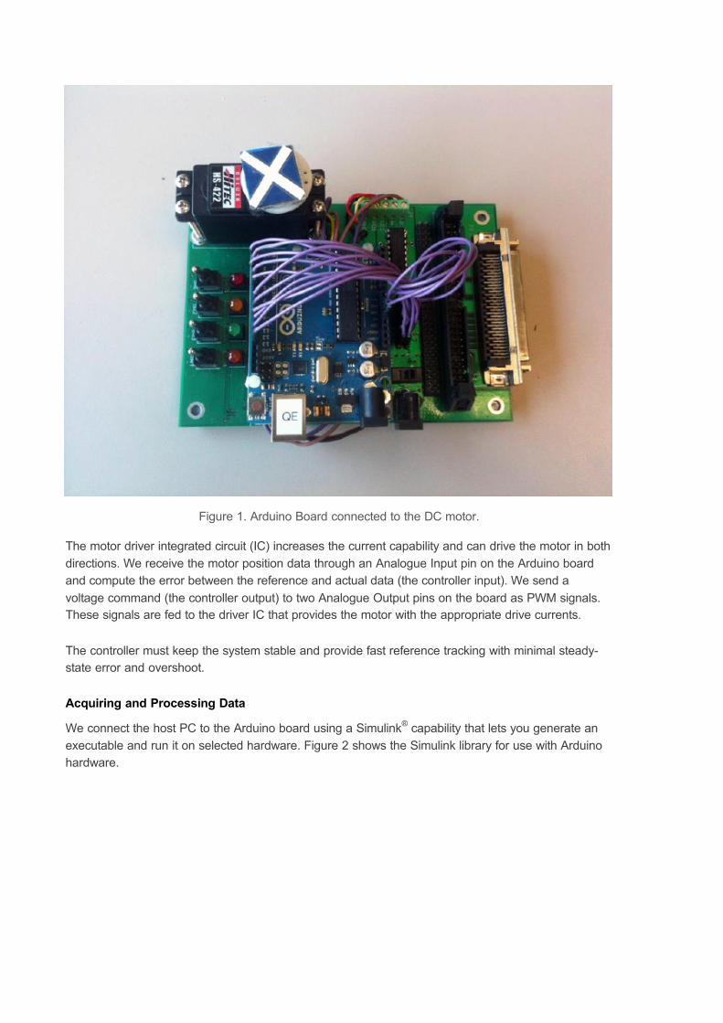
The physical system is a DC motor connected to an Arduino® Uno board via a motor driver (Figure 1).

We want to design a feedback controller for this motor to track a reference position. The controller will

generate the appropriate voltage command based on the motor position reference data. When

applied to the motor, this voltage will cause the motor to generate the torque that turns the motor shaft.

We will use a potentiometer to measure the angle of rotation of the motor shaft, and feed this angleback to the controller.



Figure 1. Arduino Board connected to the DC motor.

The motor driver integrated circuit (IC) increases the current capability and can drive the motor in both

directions. We receive the motor position data through an Analogue Input pin on the Arduino board

and compute the error between the reference and actual data (the controller input). We send a

voltage command (the controller output) to two Analogue Output pins on the board as PWM signals.

These signals are fed to the driver IC that provides the motor with the appropriate drive currents.

The controller must keep the system stable and provide fast reference tracking with minimal steady-

state error and overshoot.

Acquiring and Processing Data

We connect the host PC to the Arduino board using a Simulink® capability that lets you generate an

executable and run it on selected hardware. Figure 2 shows the Simulink library for use with Arduino

hardware.



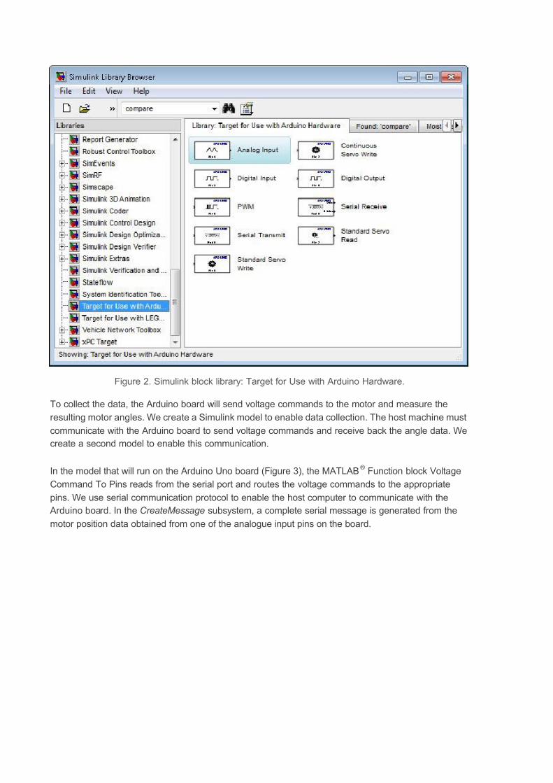
Figure 2. Simulink block library: Target for Use with Arduino Hardware.

To collect the data, the Arduino board will send voltage commands to the motor and measure the

resulting motor angles. We create a Simulink model to enable data collection. The host machine must

communicate with the Arduino board to send voltage commands and receive back the angle data. We

create a second model to enable this communication.

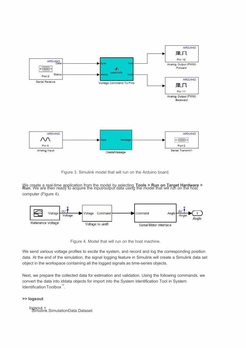
In the model that will run on the Arduino Uno board (Figure 3), the MATLAB® Function block Voltage

Command To Pins reads from the serial port and routes the voltage commands to the appropriate

pins. We use serial communication protocol to enable the host computer to communicate with the

Arduino board. In the CreateMessage subsystem, a complete serial message is generated from the

motor position data obtained from one of the analogue input pins on the board.



Figure 3. Simulink model that will run on the Arduino board.

We create a real-time application from the model by selecting Tools > Run on Target Hardware >Run. We are then ready to acquire the input/output data using the model that will run on the host

computer (Figure 4).

Figure 4. Model that will run on the host machine.

We send various voltage profiles to excite the system, and record and log the corresponding position

data. At the end of the simulation, the signal logging feature in Simulink will create a Simulink data set

object in the workspace containing all the logged signals as time-series objects.

Next, we prepare the collected data for estimation and validation. Using the following commands, we

convert the data into iddata objects for import into the System Identification Tool in System

Identification Toolbox™

.

>> logsout

logsout =Simulink.SimulationData.Dataset



Package: Simulink.SimulationData

Characteristics:

Name: 'logsout'

Total Elements: 2

Elements:

1: 'Voltage'

2: 'Angle'

-Use getElement to access elements by index or name.

-Use addElement or setElement to add or modify elements.

Methods, Superclasses

>> u = logsout.getElement(1).Values.Data;

>> y = logsout.getElement(2).Values.Data;

>> bounds1 = iddata(y,u,0.01,'InputName','Voltage','OutputName','Angle',......'InputUnit','V','OutputUnit','deg')

Time domain data set with 1001 samples.

Sample time: 0.01 seconds

Outputs Unit (if specified)

Angle deg

Inputs Unit (if specified)

Voltage V

We will be working with 12 data sets. These data sets were selected to ensure adequate excitation of

the system and to provide sufficient data for model validation.

Developing Plant Models from Experimental Data

Developing plant models using system identification techniques involves a tradeoff between model

fidelity and modelling effort. The more accurate the model, the higher the cost in terms of effort and

computational time. The goal is to find the simplest model that will adequately capture the dynamics

of the system.

We follow the typical workflow for system identification: We start by estimating a simple linear system

and then estimate a more detailed nonlinear model that is a more accurate representation of the

motor and captures the nonlinear behaviour. While a linear model might suffice for most controller

design applications, a nonlinear model enables more accurate simulations of the system behaviour

and controller design over a range of operating points.

Linear System Identification

Using the iddata objects, we first estimate a linear dynamic model for the plant as a continuous-time

transfer function. For this estimation, we specify the number of poles and zeros. System Identification

Toolbox then automatically determines their locations to maximise the fit to the selected data sets.

We launch the System Identification Tool by executing

>> ident

http://www.mathworks.com.au/company/newsletters/articles/data-sets-for-motor-control-with-arduino.html






We can import the data sets into the tool from the base workspace using the Import Data pull-down

menu (Figure 5). We also have the option to preprocess the imported data. To start the estimation

process, we select the working data that will be used to estimate a model and the validation data

against which the estimated model will be tested. We can use the same data set for both estimation

and validation initially, and then use other data sets to confirm our results. Figure 5 shows the System

Identification Tool with the data set imported. The estimation data set, data set 11, comes from an

experiment designed to avoid exciting nonlinearities in the system.

Figure 5. The System identification Tool with data imported.

We can now estimate a continuous transfer function for this data. In our example, we estimate a 2-

pole, no-zero, continuous-time transfer function (Figure 6).

Figure 6. Continuous Transfer Function estimation GUI.

We compare the simulation response of the estimated model against measured data by checking the

Model Output box in the System Identification Tool. The fit between the response of the estimated

linear model and the estimation data is 93.62% (Figure 7).

http://www.mathworks.com.au/cmsimages/74128_wm_Dataset_11_wl.jpg






Figure 7. Plot comparing estimated model response and estimation data.

To ensure that the estimated transfer function represents the motor dynamics, we must validate it

against an independent data set. For this purpose we select data set 12, where the motor operates

linearly as our validation data. We achieve a reasonably accurate fit (Figure 8).







Figure 8. Plot comparing estimated model response with validation data.

While the fit is not perfect, the transfer function that we identified does a good job of capturing the

dynamics of the system. We can use this transfer function to design a controller for the system.

We can also analyse the effect of plant uncertainty. Models obtained with System IdentificationToolbox contain information not only about the nominal parameter values but also about parameter

uncertainty encapsulated by the parameter covariance matrix. A measure of the reliability of the

model, the computed uncertainty is influenced by external disturbances affecting the system,

unmodelled dynamics, and the amount of collected data. We can visualise the uncertainty by plotting

its effect on the model’s response. For example, we can generate the Bode plot of the estimated

transfer function showing 1 standard deviation confidence bound around the nominal response

(Figure 9).

Figure 9. Bode plot of the estimated model showing model uncertainty.

Nonlinear System Identification

A linear model of the motor dynamics, created by using data collected from a linear region of its

operation, is useful for designing an effective controller. However, this plant model cannot capture

nonlinear behaviour exhibited by the motor. For example, data set 2 shows that the motor’s response

saturates at about 100°, and data set 3 shows that the motor is not responsive to small command

voltages, perhaps owing to dry friction.











In this step, we will create a higher-fidelity model of the DC motor. To do that, we estimate a nonlinear

model for the DC motor. A closer inspection of the data reveals that the change in the slope of the

response is not linearly related to the change in voltage. This trend suggests nonlinear, hysteresis-like

behaviour. Nonlinear ARX (NLARX) models offer considerable flexibility, enabling us to capture such

behaviour using a rich set of nonlinear functions, such as wavelets and sigmoid networks.

Furthermore, these models let us incorporate what we have discovered about the system

nonlinearities using custom regressors.

For the NLARX modelling to be effective, we need data that is rich in information about the

nonlinearities. We merge three data sets to create the estimation data. We merge five other data sets

to create a larger, multi-experiment, validation data set.

>> mergedD = merge(z7,z3,z6)

Time domain data set containing 3 experiments.

Experiment Samples Sample Time

Exp1 5480 0.01Exp2 980 0.01

Exp3 980 0.01

Outputs Unit (if specified)

Angle deg

Inputs Unit (if specified)

Voltage V

>> mergedV = merge(z1,z2,z4,z5,z8);

The nonlinear model had various adjustable components. We adjusted the model orders, delays, type

of nonlinear function, and the number of units in the nonlinear function. We added regressors that

represent saturation and dead-zone behaviour. After several iterations, we chose a model structure

that employed a sigmoid network with a parallel linear function and used a subset of regressors as its

inputs. The parameters of this model were estimated to achieve the best possible simulation results

(Figure 10).

http://www.mathworks.com.au/cmsimages/74028_wm_Datafit_Estimation_wl.jpg



http://www.mathworks.com.au/cmsimages/74029_wm_Datafit_Validation_wl.jpg







Figure 10. Nonlinear ARX model estimation GUI.

The resulting model has an excellent fit of >90% for the estimation data as well as for the validation

data. This model can be used for controller design as well as for analysis and prediction.

Designing the Controller

We are now ready to design a PID controller for the higher-fidelity nonlinear model. We linearise the

estimated nonlinear model at an operating point of interest and then design a controller for this

linearised model.

We tune the PID controller and then select its parameters (Figure 11).



Figure 11. PID Tuner interface.

We also check how this controller performs on the nonlinear model. Figure 12 shows the Simulink

model that we use to obtain the simulation response of the nonlinear ARX model.

Figure 12. Simulink model for testing the controller on the estimated nonlinear model.

We then compare the linearised and nonlinear model closed-loop step responses for a desiredreference position of 60° (Figure 13).



Figure 13. Step response plot comparing simulation responses of nonlinear and linearised models.

Testing the Controller on Hardware

We create a Simulink model with the controller and place it on the Arduino Uno board using Simulink

built-in support for deploying models to target hardware (Figure 14).



Figure 14. Model with the controller implemented on the Arduino board. The subsystem Get Anglereceives the reference signal from the serial port and converts it to the desired angle of the motor.

The DC Motor subsystem configures the Arduino board to interface with the physical motor.

We designed a controller by linearising the estimated nonlinear ARX model about a certain operating

point. The results for this controller show that the hardware response is quite close to the simulation

results (Figure 15).

Figure 15. Plot comparing simulation and hardware responses to a step reference for a controllerdesigned using a linearised model.



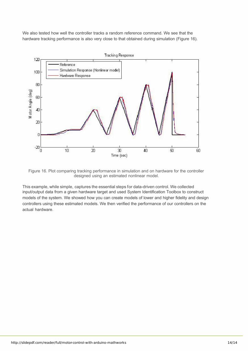
We also tested how well the controller tracks a random reference command. We see that the

hardware tracking performance is also very close to that obtained during simulation (Figure 16).

Figure 16. Plot comparing tracking performance in simulation and on hardware for the controllerdesigned using an estimated nonlinear model.

This example, while simple, captures the essential steps for data-driven control. We collected

input/output data from a given hardware target and used System Identification Toolbox to construct

models of the system. We showed how you can create models of lower and higher fidelity and design

controllers using these estimated models. We then verified the performance of our controllers on the

actual hardware.

Documents

Motor Control With Arduino MathWorks