Moving Aerial Base Station Networks: Stochastic Geometry ...Moving Aerial Base Station Networks: Stochastic Geometry Analysis and Design Perspective S. Enayati, H. Saeedi, H. Pishro-Nik,

ACCEPTED FOR PUBLICATION IN IEEE TRANSACTIONS ON WIRELESS COMMUNICATIONS, MARCH 2019 1

Moving Aerial Base Station Networks: Stochastic

Geometry Analysis and Design Perspective

S. Enayati, H. Saeedi, H. Pishro-Nik, and H. Yanikomeroglu

Abstract

Recently, the utilization of aerial base stations (ABSs) has attracted a lot of attention. For static

implementation of ABSs, it has been shown that if the ABSs are statistically distributed in a given height

over a cell, according to a binomial point process (BPP), a fairly uniform coverage across the cell is

achievable. However, such a static deployment exhibits a poor performance in terms of average fade

duration (AFD) for the static or low speed moving users and power consumption. Therefore, considering

a network of moving ABSs is of practical importance. On the other hand, once such a moving ABS

network is considered, the coverage probability may not necessarily remain at an acceptable level. This

paper is concerned with the design of stochastic trajectory processes such that if according to which

the ABSs move, in addition to improving the AFD, an acceptable coverage profile can be obtained. We

propose two families of such processes, namely spiral and oval processes, and analytically demonstrate

that the same coverage as the static case is achievable. We then focus on two special cases of such

processes, namely, radial and ring processes, and show that the AFD is reduced about two orders

of magnitude with respect to the static case. To obtain a more practical scenario, we also consider

deterministic counterparts of the proposed radial and ring processes and show that similar coverage and

AFD as the stochastic case can be obtained.

S. Enayati and H. Saeedi are with ECE Department, Tarbiat Modares University, Tehran, 14115, Iran. H. Pishro-Nik is with

ECS Department, University of Massachusetts, Amherst, MA, 01003, USA. H. Yanikomeroglu is with SCE Department, Carleton

University, Ottawa, ON, K1S 5B6, Canada. The corresponding author is H. Saeedi, email: {[email protected]}. The materiel of

this paper has been presented in part at International Symposium on Information Theory (ISIT), July 2018, Vail, CO, USA [1].


I. INTRODUCTION

Thanks to the recent advances in electronics and hardware technologies, communication, em-

bedded systems, sensor and energy storage technologies as well as carbon fiber-reinforced plastic

materials [2], low cost and easy deployment, unmanned aerial systems (UASs) have become one

of the most attractive candidates to support and complement the present and upcoming wireless

networks in different applications ranging from data collection and environment monitoring to

performing as relays and aerial base stations (ABSs) in order to enhance the network coverage

and throughput [3], [4].

ABSs can be both deployed statically or mobile. Although managing a static ABS network

may be more appealing, two major advantages come with a network of moving ABSs. First,

it has been generally stated in the literature that moving UASs outperform fixed ones as far

as the energy consumption is concerned [5]–[7]. Another benefit of having moving ABSs is

the significant reduction in average fade duration (AFD). This is defined as the average time

between entering a fading situation and going out of it, and directly depends on the receiver

and transmitter mobility. Intuitively, moving ABSs are expected to provide shorter AFD than

static ABSs. In particular, for a strictly static ABS network, a fixed user can stay in a deep fade

forever [8].

Several research directions on ABSs are in place including performance analysis [5], [9]–[13],

optimal positioning [14]–[20], and path planning [6], [21]–[25]. As far as performance analysis

is concerned, [9] investigated the coverage and rate performance of a network using an ABS

serving cellular users affected by underlaid device-to-device (D2D) users. A throughput-delay

trade-off has been considered in a throughput maximum-minimum problem in [10] to optimally

allocate time to several ground terminals while the ABS is moving along a certain straight line

in a cyclical time division manner. Assuming an ABS that relays data between a transmitter and


receiver in a circular path, the authors of [5] considered the variable rate protocol implementation

to both the transmitter-relay and relay-receiver links in order to investigate outage probability

and achievable rate. Furthermore, using the tools from the stochastic geometry, [11] and [13]

provided coverage and throughput analysis in a Binomial point process (BPP) and Poisson point

process (PPP) modeled networks of static ABSs, respectively. Also, [26] proposed a stochastic

model for ABS networks which considers both the ABS-user link and the ABS-backhaul link

simultaneously.

In papers considering the optimal deployment, the goal is often to optimize the placement of

the ABSs to provide satisfaction in a variety of quality of service (QoS) levels. In this regard, [14]

optimizes the distance between two ABSs in two cases of having and not-having interference

to obtain a certain coverage probability in a given area. In [15], assuming only a line-of-sight

(LoS) dominated channel, simulation based sequential algorithms have been presented to obtain

the minimum number of ABSs and their placement to cover a given area. In a similar work, [16]

obtained the minimum number and the optimal 3D placement of the ABSs using the particle

swarm optimization (PSO) algorithm. The authors in [17] optimized the 3D location of multiple

ABSs using circle packing theory that led to a maximum coverage and minimum transmit power

for the ABSs. The same authors in [18] and [19] proposed a cell association algorithm using

the optimal transport theory while considering the terrestrial base stations in the latter.

As the mobility is the unique feature of the ABSs compared to their counterpart, i.e., terrestrial

base stations, it is not surprising that many studies have recently been devoted to this aspect.

In particular, path planning problems have been proposed in which, similar to the previous

category, the goal is to design an optimal path to satisfy certain QoS indicators. In [6] after

deriving a theoretical model for the propulsion energy consumption, the authors investigated the

energy efficiency problem in a certain circular trajectory and a general trajectory of a single


ABS. Movement minimization of data collecting ABSs to obtain the optimum trajectory was

considered in [21], where the authors are also willing to make the power transmission of Internet

of things (IoT) devices more efficient. In [22], the user scheduling and a single ABS trajectory

were jointly optimized with the objective of maximizing the minimum average sum rate. A

similar idea was considered in [23] for the multi-ABS case. A recent trajectory planning was

investigated in [24] in which a single UAV is considered to help a ground BS while turning a

circular path around it with a constant speed. A similar trajectory was considered in [25], where

for a multiple antenna equipped UAV, the transmission duration and the transmit power were

jointly optimized to obtain the maximum data collection efficiency.

As can be seen, many works have dealt with moving ABSs, most of which deal with finding

optimal trajectory paths with different utility functions such as sum-rate or energy efficiency,

e.g., [6], and [21]–[25], [27]. However, there is no work in multi UAV network in the literature

that uses coverage probability as the utility function as it can result in intractable and compli-

cated optimization problems. Moreover, even for deterministic utility functions, the optimization

problems are sometimes so complicated to solve that many works investigate a network with

a single ABS [22], [24], [25], [28]–[31] and in many cases, it is assumed that we know the

locations of the users and/or other elements of the network, e.g., [31], [32]–[34]. In this paper,

we aim to present a different perspective on the motion analysis of the ABSs. Our scheme

makes it possible to deal with probabilistic measures such as coverage probability and there

is no limitation in analyzing multiple ABSs and mobile users. Such a stochastic analysis has

been applied widely to several cellular network frameworks, see, e.g., [35]–[37] and references

therein.

As far as ABS networks are concerned, stochastic geometry analysis has already been applied

to a network of fixed ABSs [11]. In this work, the ABSs are modeled according to a uniform BPP


and then the closed-form formulations for coverage probability are obtained. Analysis shows that

such a BPP distribution for ABSs can provide fairly uniform coverage across the cell and the

outage probability can be maintained below an acceptable value throughout the cell. However, if

the ABSs are assumed to be moving, this is not the case anymore necessarily. For example, let’s

assume ABSs start their flight with constant speed from the cell center towards the cell edge in

straight lines with an angle uniformly chosen with respect to the X axis and return on the same

line before they choose a new angle and leave the origin again at another random angle. This

can be seen as one of the simplest trajectories that comes to mind. After few departures/arrivals

from/to the origin, this moving pattern leads ABSs to be concentrated at the cell center which

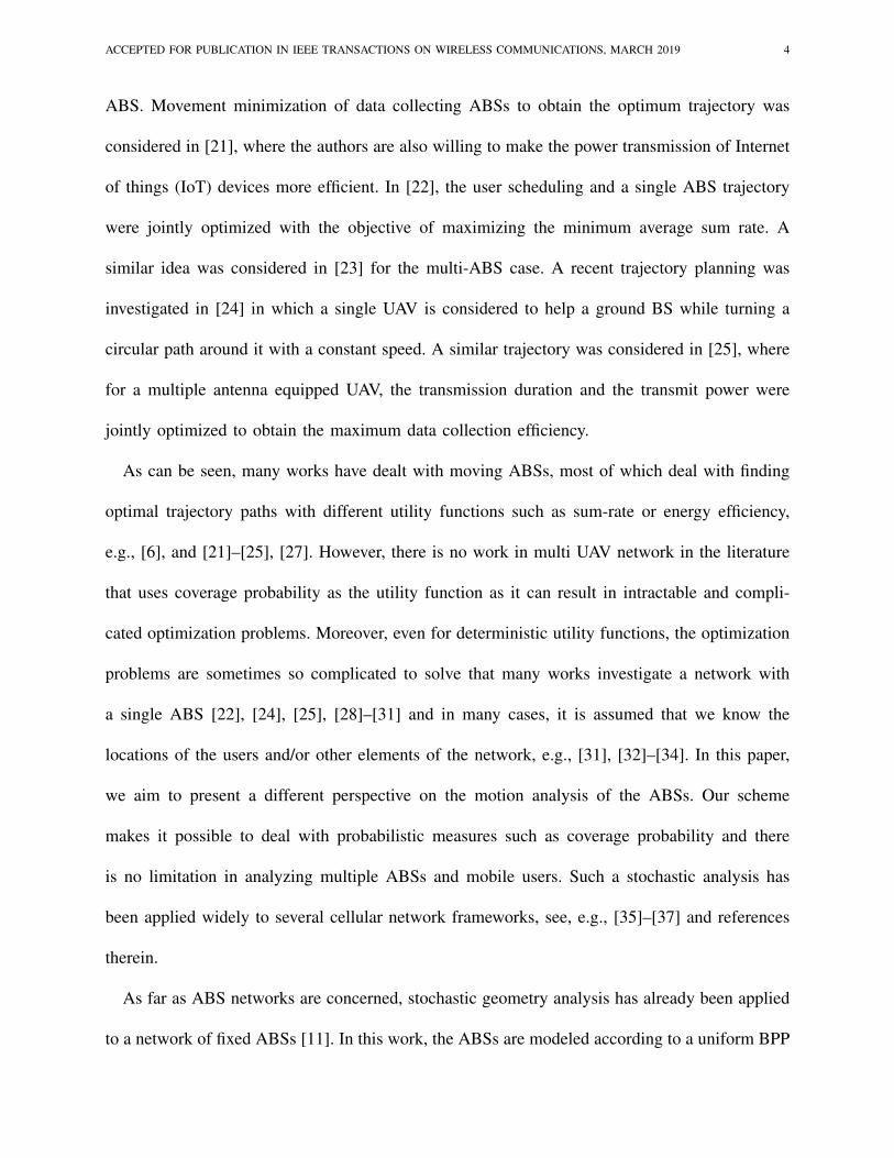
results in the coverage probability degradation at the cell edge. In Fig. 1, we have compared

the coverage profile resulting from the considered moving pattern to the coverage obtained by

deploying BPP-distributed static ABSs. As can be seen, the coverage probability at the cell edge

is not acceptable for the moving case.1

In this paper, our aim is to design a family of trajectory processes that if according to which

te ABSs move, a fairly uniform user coverage can be maintained while taking advantage of

the benefits of ABS mobility. The results are promising: we analytically demonstrate that the

proposed family of trajectory processes can maintain the same coverage behavior as that of the

uniform BPP. Through simulation, we observe significant improvement in the AFD compared

to the static case. This is in addition to the saving we obtain in energy consumption as stated

in the literature2.

The obtained stochastic trajectory curves are then used as a building block to design determin-

1In addition to the results of the figure, the non-uniformity of the points in the case of constant speed can be proved analytically.

We have not stated the proof here due to space limitation.

2This statement regarding the energy comes from [5]–[7] and is not simulated in this paper.


User location (m)0 500 1000 1500 2000 2500 3000 3500 4000

Cov

erag

e pr

obab

ility

0

0.1

0.2

0.3

0.4

0.5

0.6

0.7

0.8

0.9

1

Static BPPMoving ABS with uniform velocity

Fig. 1. Coverage probability vs. distance to origin for a cell with radius ρ = 4 km and 10 ABSs. For static case, ABSs are

distributed according to BPP. For the mobile case, the ABSs move with a constant speed of 5 m/s.

istic trajectory curves that are practically implementable. We show that with reasonable number

of ABSs, we can obtain similar AFD and coverage probability as that of the stochastic case

without the ABSs being moving in stochastic paths.

This paper is organized as follows: in Section II, we revisit some existing definitions and

formulations for coverage probability in a finite network of ABSs. In Section III, we introduce

two general family of stochastic trajectory processes and their corresponding special cases as

well as the deterministic design. Section IV provides simulation results and Section V concludes

the paper.

Notations: In this paper, deterministic quantities are denoted by italic letters, while stochastic

quantities are denoted by bold-face lower-case and upper-case letters.

II. SYSTEM MODEL AND PRELIMINARIES

In this section, we review the concept of general BPP and uniform BPP. Then, we explain

the system model and review the formulations for the coverage probability corresponding to a

network in which the ABSs are modeled as a BPP. If a fixed number of points are independently


and identically distributed (i.i.d.) on a compact set W ∈ Rd [38], we say the points can be

modeled as a general BPP. If these points are distributed uniformly within the same compact

set, then we say the points are modeled according to a uniform BPP .

Now suppose that N ABSs at height H are distributed according to a BPP in a circle

with radius of ρ and start their flights independently following an arbitrary trajectory process,

{X1(t),X2(t),X3(t), · · ·}, at times T1,T2, ...,TN , chosen uniformly and independently from

(0, τ), respectively, according to a given PDF (it is assumed that the trajectory curves are chosen

independently from a certain probability space, and are independent from the starting times

T1,T2, ...,TN ). It can be easily seen that at any arbitrary observation time of t′ ≥ τ , the ABSs

still follow a general BPP. However, if these ABSs are distributed according to uniform BPP and

move according to an arbitrary trajectory, at a given time instant, then ABSs do not necessarily

follow a uniform BPP model.

We assume that N ABSs are BPP-distributed at the fixed height of H above a circular area

of radius ρ, referred to as cell3. The ABSs can be static or moving. At any time snapshot, the

aim is to provide coverage for the user located at a given point (x0, 0, 0). We assume that the

user is connected to its closest ABS, called the serving ABS where the instantaneous distance

between the serving ABS and the user is denoted by r. Note that in a dynamic network, the user

can be handed over to a different ABS based on the change in the value of r. Assuming ABSs

share the same resource blocks in time or frequency with a reuse factor of 1, the other ABSs

are considered as interfering ABSs. Alternatively, we can assume that the spectrum is divided

between the ABS’s.

Using the formulation of [11] for the case of uniform BPP, we can revisit the following

proposition corresponding to the coverage probability for the case of uniform BPP:

3In this paper by cell, we mean a circular area without any ground base stations that aims to be covered by a set of ABSs.


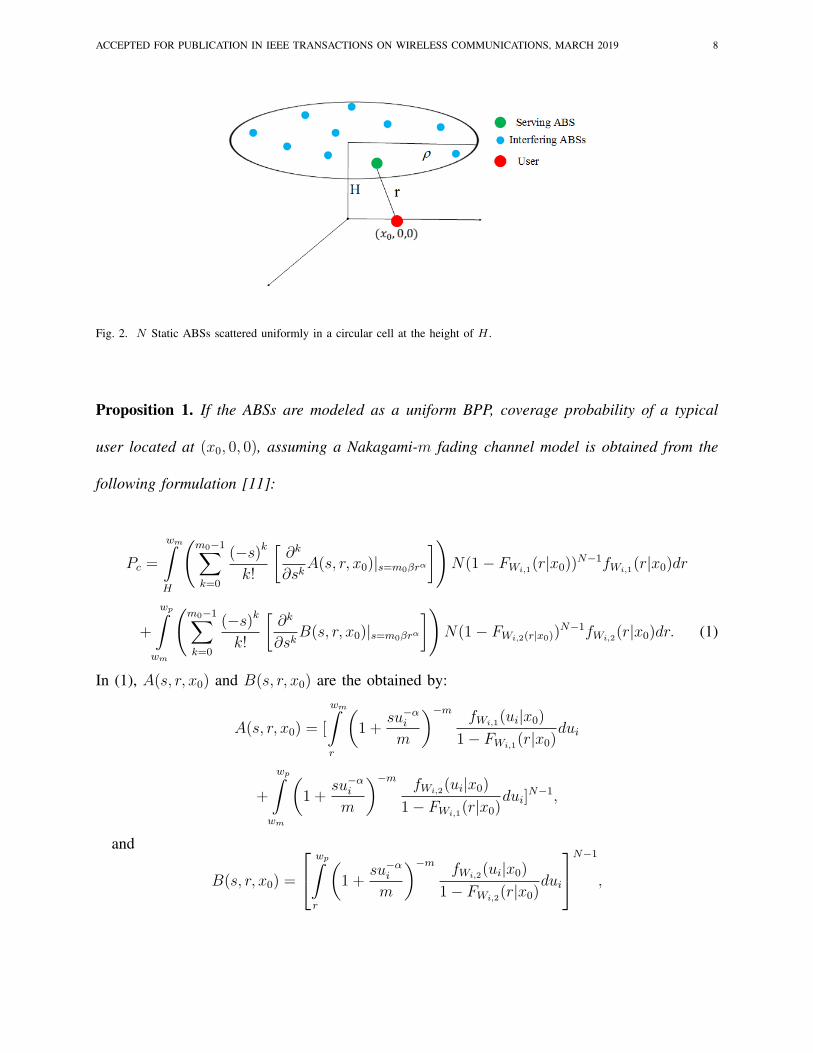
Fig. 2. N Static ABSs scattered uniformly in a circular cell at the height of H .

Proposition 1. If the ABSs are modeled as a uniform BPP, coverage probability of a typical

user located at (x0, 0, 0), assuming a Nakagami-m fading channel model is obtained from the

following formulation [11]:

Pc =

wm∫H

(m0−1∑k=0

(−s)k

k!

[∂k

∂skA(s, r, x0)|s=m0βrα

])N(1− FWi,1

(r|x0))N−1fWi,1

(r|x0)dr

+

wp∫wm

(m0−1∑k=0

(−s)k

k!

[∂k

∂skB(s, r, x0)|s=m0βrα

])N(1− FWi,2(r|x0))

N−1fWi,2(r|x0)dr. (1)

In (1), A(s, r, x0) and B(s, r, x0) are the obtained by:

A(s, r, x0) = [

wm∫r

(1 +

su−αi

m

)−m fWi,1(ui|x0)

1− FWi,1(r|x0)

dui

+

wp∫wm

(1 +

su−αi

m

)−m fWi,2(ui|x0)

1− FWi,1(r|x0)

dui]N−1,

and

B(s, r, x0) =

wp∫r

(1 +

su−αi

m

)−m fWi,2(ui|x0)

1− FWi,2(r|x0)

dui

N−1

,


respectively, where FWi,1(r|x0) and FWi,2

(r|x0) are the cumulative distribution functions (CDF)s

of the distances from the receiver to the ABSs denoted by {Wi} conditioned on x0 given as

below:

FWi,1(r|x0) =

r2 −H2

ρ2,

FWi,2(r|x0) =

r2 −H2

πρ2(θ∗ − 0.5 sin 2θ∗) +

1

π(ϕ∗ − 0.5 sin 2ϕ∗) ,

where

θ∗ = arccos

(r2 + x0

2 − d2

2x0

√r2 −H2

),

and

ϕ∗ = arccos

(x0

2 + d2 − r2

2x0ρ

).

Also, fWi,1(ui|x0) and fWi,2

(ui|x0) are the set of distance probability distribution functions

(PDF)s of ABSs conditioned on x0 given by:

fWi,1(ui|x0) =

2ui

ρ2,

and

fWi,2(ui|x0) =

2ui

πρ2arccos

(ui

2 + x02 − d2

2x0

√ui

2 −H2

).

Furthermore, wm =√

(ρ− x0)2 +H2, wp =√

(ρ+ x0)2 +H2, and d =√

ρ2 +H2, β is the

signal-to-interference ratio (SIR) threshold, α > 2 is the path-loss exponent, and m0 and m are

the Nakagami-m parameters of the serving and interfering links, respectively. A key feature of

ABSs is their ability to change altitude. However, considering this extra degree of freedom adds

to the complexity of an already involved design problem. Therefore, in this paper, we assume

all ABSs fly in a fixed altitude. Also, in most countries, the existing policies impose important

restrictions to the height and UAV may end up flying at a limited range altitude.


III. STOCHASTIC TRAJECTORY PROCESSES THAT PROVIDE UNIFORM COVERAGE

A. General Idea and Summary of Results

In the previous section, we reviewed the result of [11] in which for a network of static ABSs

modeled according to uniform BPP, closed-form formulations for coverage were obtained. As

shown in Fig. 1, such a distribution provides fairly uniform coverage across the cell but as

long as the ABSs are static, the user experience in terms of AFD is poor. In the same figure,

we observed that if the ABSs start moving, while the AFD experience may improve, such a

uniformity in coverage is not necessarily preserved. Therefore in this section, we are looking

for trajectory processes such that if according to which the ABSs move, the points remain to

follow BPP at any time instant, leading to an almost uniform coverage. So far, we have been

able to identify two families of such trajectory processes, referred to as spiral and oval trajectory

processes.

Before getting involved with the detailed analytical formulations and their derivations, we

provide an intuitive summary first. As mentioned above, we have identified two major families

of processes, namely, spiral and oval. In spiral trajectory processes, each ABS generally starts

flying from the cell origin towards the cell edge according to the specs itemized in Definition

1 of the next subsection. An important member of this family is called the radial trajectory

process in which the trajectories are in fact the cell radius. In oval trajectory processes, each

ABS moves on a closed curve, containing the cell origin within it according to the specs itemized

in Definition 2 of the next subsection. An important member of this family is called the ring

trajectory process in which the trajectories are in fact randomly-selected cell radii, all centered

at the cell origin.

An important question that may arise is how to implement such stochastic moving paths

in a deterministic way. To address this question, by focusing on the radial and ring trajectory


x (km)-5 -4 -3 -2 -1 0 1 2 3 4 5

y (k

m)

-4

-3

-2

-1

0

1

2

3

4

ABS1, ∆θ1 = 2π/5, v

1 = ρ2/τR

1

ABS2, ∆θ2 = 2π/5, v

2 = ρ2/τR

2

ABS3, ∆θ3 = 2π/5, v

3 = ρ2/τR

3

ABS4, ∆θ4 = 2π/5, v

4= ρ2/τR

4

ABS5, ∆θ5 = 2π/5, v

5 = ρ2/τR

5

∆θ5

∆θ4

∆θ3

∆θ1

∆θ2

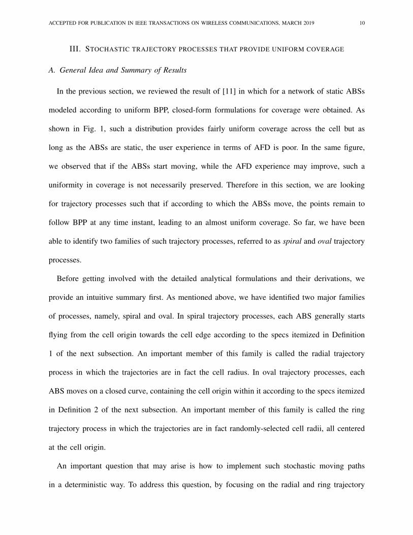
Fig. 3. ABSs location according to deterministic radial trajectory in a cell of radius 4 km.

processes, we introduce their deterministic counterparts and show that they also provide similar

behavior in terms of coverage and AFD to the stochastic case.

For the deterministic radial trajectory, we claim that we can achieve the required uniform

coverage with N available ABSs across a cell of radius ρ, if they are scheduled to move as

follows:

1- For an arbitrary initial phase β, the ith ABS will fly on a radius with phase β+2π(i−1)/N .

2- For an arbitrary constant value τ , all ABSs fly with similar speed profiles, vi = ρ2

Riτ, where

Ri is the instantaneous distance to the origin.

3- The ith ABS departs origin at time iτ/(N + 1).

4- Once any ABS reaches the edge of the cell, it reverses its direction and returns to the origin

with the same speed profile as in Item 2 and this cycle continues periodically.

Fig. 3 shows a snapshot of the ABSs’ coordinates in a cell with radius of 4 km, for N = 5.

For the deterministic ring trajectory, we claim that we can achieve the required uniform

coverage with N available ABSs across a cell of radius ρ, if they are scheduled to move as

follows:


x (km)-5 -4 -3 -2 -1 0 1 2 3 4 5

y (k

m)

-4

-3

-2

-1

0

1

2

3

4ABS1, R

12 = 1/6 ρ2, ∆ θ

1=2π/5

ABS2, R22 = 2/6 ρ2, ∆ θ

2=2π/5

ABS3, R32 = 3/6 ρ2, ∆ θ

3=2π/5

ABS4, R42 = 4/6 ρ2, ∆ θ

4=2π/5

ABS5, R52 = 5/6 ρ2, ∆ θ

5=2π/5

∆ θ1

∆ θ2

∆ θ3

∆ θ4

∆ θ5

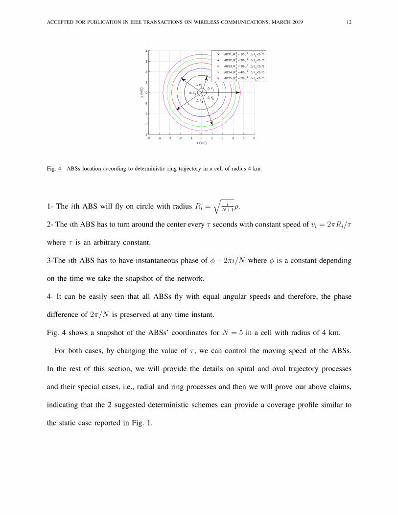
Fig. 4. ABSs location according to deterministic ring trajectory in a cell of radius 4 km.

1- The ith ABS will fly on circle with radius Ri =√

iN+1

ρ.

2- The ith ABS has to turn around the center every τ seconds with constant speed of vi = 2πRi/τ

where τ is an arbitrary constant.

3-The ith ABS has to have instantaneous phase of ϕ+ 2πi/N where ϕ is a constant depending

on the time we take the snapshot of the network.

4- It can be easily seen that all ABSs fly with equal angular speeds and therefore, the phase

difference of 2π/N is preserved at any time instant.

Fig. 4 shows a snapshot of the ABSs’ coordinates for N = 5 in a cell with radius of 4 km.

For both cases, by changing the value of τ , we can control the moving speed of the ABSs.

In the rest of this section, we will provide the details on spiral and oval trajectory processes

and their special cases, i.e., radial and ring processes and then we will prove our above claims,

indicating that the 2 suggested deterministic schemes can provide a coverage profile similar to

the static case reported in Fig. 1.


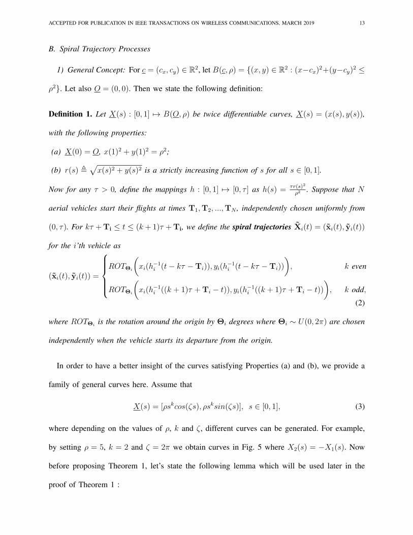
B. Spiral Trajectory Processes

1) General Concept: For c = (cx, cy) ∈ R2, let B(c, ρ) = {(x, y) ∈ R2 : (x−cx)2+(y−cy)

2 ≤

ρ2}. Let also O = (0, 0). Then we state the following definition:

Definition 1. Let X(s) : [0, 1] 7→ B(O, ρ) be twice differentiable curves, X(s) = (x(s), y(s)),

with the following properties:

(a) X(0) = O, x(1)2 + y(1)2 = ρ2;

(b) r(s) ≜√x(s)2 + y(s)2 is a strictly increasing function of s for all s ∈ [0, 1].

Now for any τ > 0, define the mappings h : [0, 1] 7→ [0, τ ] as h(s) = τr(s)2

ρ2. Suppose that N

aerial vehicles start their flights at times T1,T2, ...,TN , independently chosen uniformly from

(0, τ). For kτ +Ti ≤ t ≤ (k+1)τ +Ti, we define the spiral trajectories Xi(t) = (xi(t), yi(t))

for the i’th vehicle as

(xi(t), yi(t)) =

ROTΘi

(xi(h

−1i (t− kτ −Ti)), yi(h

−1i (t− kτ −Ti))

), k even

ROTΘi

(xi(h

−1i ((k + 1)τ +Ti − t)), yi(h

−1i ((k + 1)τ +Ti − t))

), k odd,

(2)

where ROTΘiis the rotation around the origin by Θi degrees where Θi ∼ U(0, 2π) are chosen

independently when the vehicle starts its departure from the origin.

In order to have a better insight of the curves satisfying Properties (a) and (b), we provide a

family of general curves here. Assume that

X(s) = [ρskcos(ζs), ρsksin(ζs)], s ∈ [0, 1], (3)

where depending on the values of ρ, k and ζ , different curves can be generated. For example,

by setting ρ = 5, k = 2 and ζ = 2π we obtain curves in Fig. 5 where X2(s) = −X1(s). Now

before proposing Theorem 1, let’s state the following lemma which will be used later in the

proof of Theorem 1 :


x(s)-6 -4 -2 0 2 4 6

y(s)

-6

-4

-2

0

2

4

6X

1(s)

X2(s)

B(0,ρ)

Fig. 5. Typical curves from the spiral trajectory process with ρ = 5, k = 2 and ζ = 2π.

Lemma 1. Consider a periodic function g : R 7→ [0,∞), where g(t+τ) = g(t), ∀t ∈ R. FR(t)(r),

the CDF of the randomly shifted process R(t) ≜ g(t−T),T ∼ U(0, τ), is obtained by

FR(t)(r) =|A|τ

, (4)

where |.| is the Lebesgue measure of A defined as A = {α ∈ [0, τ ]| g(α) ≤ r}.

Proof.

FR(t)(r) =

∫ τ

0

Pr (g(t−T) ≤ r|T = α) fT(α)dα

=1

τ

∫ τ

0

1{g(t−α)≤r}dα =|A|τ

, (5)

where A is defined as the region in which g(α) ≤ r during one period, i.e., A = {α ∈

[0, τ ]|g(α) ≤ r}.

Corollary 1. If we have g(2τ − t) = g(t), t ∈ (0, τ), and R(t) ≜ g(t−T),∼ U(0, τ), we get

a similar distribution since g(t) is symmetric with respect to τ .

Now we are ready to state the following theorem:


Theorem 1. For all t > τ , the instantaneous locations of the aerial vehicles on the spiral

trajectory, i.e., Xi(t) = (xi(t), yi(t)), form a uniform BPP in B(O, ρ).

Proof. For the proof of Theorem 1, we first need to show that for t ≥ τ , the location of vehicles

are independent. This is intuitive, since Θi ∼ U(0, 2π) and Ti ∼ U(0, τ) both have been chosen

independently. Second, we have to show that the locations are uniformly distributed in B(O, ρ).

To do so, we note that since Θi ∼ U(0, 2π), the phase of an arbitrary point on the curve is

uniformly distributed between 0 and 2π, i.e., Xi(t) ∼ U(0, 2π). It only remains to show that

the CDF of the distance between the origin and an arbitrary point on the curve, i.e., ∥Xi(t)∥, is

equal to the distribution corresponding to uniform BPP within B(O, ρ). For notational simplicity,

we drop index i in the rest of the proof.

Let

u(t) ≜

∥X(h−1(t))∥ 0 ≤ t ≤ τ

∥X(h−1(2τ − t))∥ τ ≤ t ≤ 2τ

. (6)

We provide the proof for the case of 0 ≤ t ≤ τ , the proof for the case of τ ≤ t ≤ 2τ is similar.

According to (6) and Property 2 in Definition 1, we understand that

u(t) = ∥X(h−1(t))∥= r(h−1(t)). (7)

Also, since the random rotation of X(t) will not affect its absolute value, we have ∥X(t)∥=

u(t − T) where X(t) is the randomly rotated and shifted version of X(t) defined in Eq. (2).

Now using Lemma (1), we obtain F∥X∥ as below

F∥X∥ =1

τ|{0 ≤ α ≤ τ : u(α) ≤ r}|

=1

τ|{0 ≤ α ≤ τ : ∥X(h−1(α))∥≤ r}|. (8)


Again, according to Property 2, since r(s)2 is strictly increasing, h(s) = τr(s)2

ρ2is also strictly

increasing and hence, there exists an αmax such that

∥X(h−1(αmax))∥≤ r. (9)

Therefore, F∥X∥ =|[0,αmax]|

τ= αmax

τ. Now suppose there exists an arbitrary 0 ≤ α∗ ≤ τ such that

α∗ =τr2

ρ2. (10)

This means there exists a s∗ ∈ [0, 1] such that

α∗ = h(s∗) =τr∗2

ρ2, (11)

which means r∗ = r(h−1(α∗)) = r. Therefore, we have

h−1(α∗) = h−1(αmax), (12)

according to (9). By this, we can uniquely obtain α∗ = αmax, since h is monotonic. Finally, the

CDF can be written as

F∥X∥ =|{0 ≤ α ≤ αmax}|

τ=

r2

ρ2, (13)

which is the same as the CDF corresponding to a BPP within B(O, ρ). This completes the

proof.

The family of curves introduced by this theorem is quite diverse. In the next subsection, we

focus on one of the simple trajectory processes of this family called radial trajectory process.

2) Radial Trajectory Process: A sample radial trajectory process is shown in Fig. 6. It

can be obtained by setting k = 1 and ζ = 0 in (3). In this setup, we consider a cell with

radius ρ. We assume that N ABSs start to take off from the cell center at random moments

T1,T2, ...,TN ∈ (0, τ) where τ is the initialization time in which all N ABSs start to take

off. T1,T2, ...,TN are independently chosen uniformly from (0, τ). Each ABS first flies to a


𝜃1 𝜃2

𝜃𝑖

𝑟1(𝑡)

𝑟2(𝑡)

𝑖 = 1,2,… ,𝑁

ABS

𝜃𝑖~𝑈(0,2𝜋)

ρ

𝑟𝑖(𝑡)

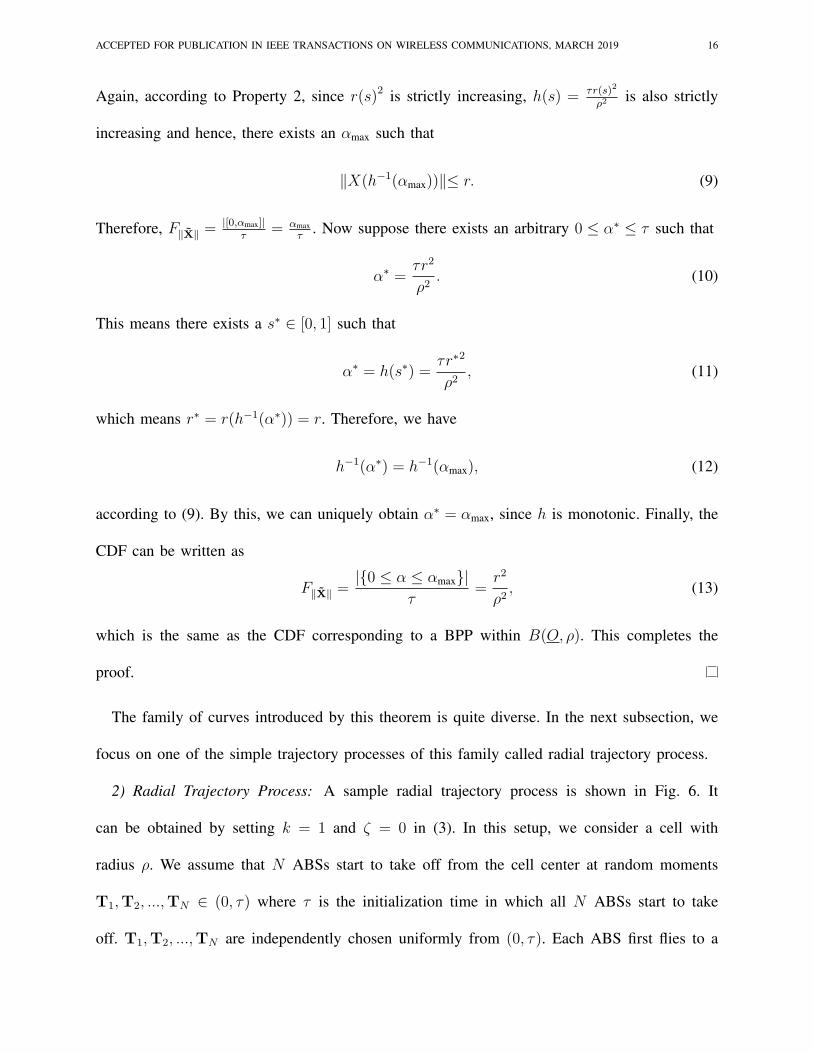
Fig. 6. An illustration of flying ABSs according to a radial trajectory process.

predetermined altitude of H and then chooses a random angle Θi ∈ (0, 2π) uniformly and

flies in a straight line towards the cell edge where its distance to origin at time t is shown by

the random variable R(t). When an ABS reaches the cell edge, it returns to the origin on the

same angle to complete the first cycle and this action repeats continuously. For each half cycle

kτ +Ti ≤ t ≤ (k + 1)τ +Ti, R(t) has to satisfy the following formulation:

Ri(t) =

ρ√

t−Ti−kττ

, k even

ρ√

(k+1)τ+Ti−tτ

k odd

. (14)

Note that with this definition, we have Ri(kτ) = 0 if k is even and Ri(kτ) = ρ otherwise.

In other words, τ is the time it takes for an ABS to go from center to the edge. It is worth

mentioning that during the initial take off phase, it takes a while for each ABS to get to the

altitude H , but we assume this time is negligible compared to τ . By the description above, one

can understand that after the time τ , we have N ABSs flying at the altitude of H .

A very interesting point in radial trajectory process is the behaviour of the ABS velocity which


can be obtained by the taking derivative of (14):

Vi(t) =

ρ√

τ(t−Ti−kτ), k even

− ρ√τ((k+1)τ+Ti−t)

, k odd

. (15)

Eq. (15) demonstrates that as t increases (i.e., ABS is at larger distance from the center), its

velocity decreases which means that it spends longer time flying at the larger distances to provide

a uniform coverage.

C. Oval Trajectory Processes

1) General Concept:

Definition 2. For any given a, b ∈ R+, where 0 ≤ a ≤ b ≤ ρ, let Xa,b(s) : [0, 1] 7→ B(O, ρ) be

twice differentiable curves, Xa,b(s) = (xa,b1 (s), xa,b

2 (s)), with the following properties:

(a) Xa,b(0) = (0, a), Xa,b(1) = (b, 0);

(b) ra,b(s) ≜ ∥Xa,b(s)∥=√xa,b1 (s)2 + xa,b

2 (s)2 is a non-decreasing function of s for all s ∈

[0, 1].

Now, for any τ > 0, define the mappings ha,b : [0, 1] 7→ [0, τ4] as

ha,b(s) =τ(ra,b(s)− a)

4(b− a). (16)

In addition, for i ∈ {1, 2, · · · , N}, assume that random variables (Ai,Bi) are chosen inde-

pendently according a two-dimensional probability distribution that satisfies P (0 ≤ Ai ≤ Bi ≤

ρ) = 1 and

EAi,Bi

[1(Ai≤r≤Bi)

Ai −Bi

]=

2r

ρ2, for all r ∈ [0, ρ]. (17)


We define the corresponding oval trajectories Za,b(t) : [0, τ ] 7→ B(O, ρ) as in Equations (18)

and (19), for 0 ≤ t ≤ τ2

and τ2

≤ t ≤ τ , respectively:

Za,b(t) = (za,b1 (t), za,b2 (t)) =

(xa,b1 (h−1

i (t)), xa,b2 (h−1

i (t))

), for 0 ≤ t ≤ τ

4(− xa,b

1 (h−1i ( τ

2− t)), xa,b

2 (h−1i ( τ

2− t))

), for τ

4≤ t ≤ τ

2

,

(18)

Za,b(t) = (za,b1 (t), za,b2 (t)) =

(− xa,b

1 (h−1i (t− τ

2)),−xa,b

2 (h−1i (t− τ

2))

), for τ

2≤ t ≤ 3τ

4(xa,b1 (h−1

i (τ − t)),−xa,b2 (h−1

i (τ − t))

), for 3τ

4≤ t ≤ τ

.

(19)

Now for any ABS i, we set a = Ai and b = Bi to generate Za,bi (t). The extended oval trajectories,

Za,b(t) = (za,b1 (t), za,b2 (t)) : R+ 7→ B(O, ρ), are defined by periodically extending Za,b(t) outside

of [0, τ ] such that

Za,b(t+ τ) = Z

a,b(t), for t ∈ R+.

Suppose that N aerial vehicles start their flights at times T1,T2, ...,TN , independently

chosen uniformly from (0, τ). Let also WAi,Bi

i (t) be the corresponding delayed extended oval

trajectories according to Ti’s, i.e., for t ∈ [Ti,∞],

WAi,Bi(t) = ZAi,Bi

(t−Ti).

Moreover, for t > τ , we define the rotated delayed extended oval trajectories, Vi(t) =

(vi(t), vi(t)) of the i’th vehicle

(vi(t), vi(t)) = ROTΘi

(WAi,Bi(t)

), (20)

where ROTΘiis the rotation around the origin by Θi degrees and Θi ∼ U(0, 2π) is chosen

independently from each other.


x(s)-4 -3 -2 -1 0 1 2 3 4

y(s)

-4

-3

-2

-1

0

1

2

3

4a=1,b=3a=1,b=2a=2,b=3

Fig. 7. Typical curves from the oval trajectory process.

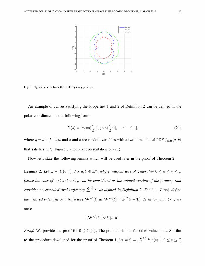
An example of curves satisfying the Properties 1 and 2 of Definition 2 can be defined in the

polar coordinates of the following form

X(s) = [q cos(π

2s), q sin(

π

2s)], s ∈ [0, 1], (21)

where q = a+(b−a)s and a and b are random variables with a two-dimensional PDF fA,B(a, b)

that satisfies (17). Figure 7 shows a representation of (21).

Now let’s state the following lemma which will be used later in the proof of Theorem 2.

Lemma 2. Let T ∼ U(0, τ). Fix a, b ∈ R+, where without loss of generality 0 ≤ a ≤ b ≤ ρ

(since the case of 0 ≤ b ≤ a ≤ ρ can be considered as the rotated version of the former), and

consider an extended oval trajectory Za,b(t) as defined in Definition 2. For t ∈ [T,∞], define

the delayed extended oval trajectory Wa,b(t) as Wa,b(t) = Za,b(t−T). Then for any t > τ , we

have

∥Wa,b(t)∥∼ U(a, b).

Proof. We provide the proof for 0 ≤ t ≤ τ4. The proof is similar for other values of t. Similar

to the procedure developed for the proof of Theorem 1, let u(t) = ∥Za,b(h−1(t))∥, 0 ≤ t ≤ τ

4


and ∥Wa,b(t)∥= u(t − T), where T is a uniform random variable in the interval (0, τ). With

these assumptions and using Lemma 1, we obtain

F∥Wa,b∥ =4|{0 ≤ β ≤ τ

4: u(β) ≤ r}|

τ

=4|{0 ≤ β ≤ τ

4: ∥Za,b

(h−1(β))∥≤ r}|τ

, (22)

where since h(s) defined in (16) is a non-decreasing function of s, we can say that there exists

a βmax for which we have ∥Za,b(h−1(βmax))∥≤ r. Hence, we get

F∥Wa,b∥ =4|[0, βmax]|

τ=

4βmax

τ. (23)

On the other hand, let 0 ≤ β∗ ≤ τ4, β∗ = τ(r−a)

4(b−a)which means there exists a s∗ ∈ [0, 1] for which

β∗ = h(s∗). Therefore, we have h−1(β∗) = h−1(βmax) and since h is monotonic, we uniquely

have β∗ = βmax. Finally we obtain the CDF of the distance between any point on the first quarter

located on the curve W a,b(t) and the origin as below

F∥Wa,b∥ =4|{0 ≤ β ≤ βmax}|

τ=

4βmax

τ=

r − a

b− a, (24)

which is the CDF of a random variable distributed uniformly between a and b.

We are now ready to state Theorem 2:

Theorem 2. For all t > τ , the instantaneous locations of the aerial vehicles on the rotated

delayed extended oval trajectory, i.e., V(t), form a uniform BPP in B(O, ρ).

Proof. Similar to the case of Theorem 1, since Θi ∈ (0, 2π) and Ti ∈ (0, τ) are each chosen

independently, we conclude that the points on the curves are independent. Now we can obtain

the distribution of distances of the points on the rotated delayed extended oval trajectory Vi(t)

for t ≥ τ , f∥V∥(r) as below

f∥V∥(r)(i)=

∫a

∫b

f∥V∥|A,B(r|a, b)fA,B(a, b)dadb


= EA,B[f∥V∥|A,B(r|a, b)](ii)= EA,B

[1A≤r≤B

B−A

], (25)

where (i) results from the law of total probability and (ii) comes from Lemma 2 where we

showed that given a and b, the distribution of ∥Wa,b(t)∥ is uniform in the interval (a, b). Finally,

according to (17) the last statement in (25) is equal to 2rρ2

and so we have f∥V∥(r) =2rρ2

which

completes the proof.

In the following, we bring up two special cases of the oval trajectory processes.

2) Ellipse and ring processes: Assume that for the ith ABS, we fix Bi = ρ and fAi(a) =

2ρ2(ρ − a) and 0 ≤ a ≤ ρ. Now, by setting b = Bi and a = Ai in (21), it reduces to an ellipse

with semi-major axis Bi and semi-minor axis Ai. To show that it is an oval trajectory, we have

to check out if (17) holds. To do so, we observe that

EAi,Bi

[1Ai≤r≤Bi

Bi −Ai

]= EAi

[1Ai≤r

ρ−Ai

]=

∫ r

0

2

ρ2(ρ− a)(ρ− a)da

=2r

ρ2, 0 ≤ r ≤ ρ, (26)

which satisfies (17). We refer to this process as the ellipse process.

Another special case can be obtained by assuming Bi to be a random variable with fBi(b) = 2b

ρ2

and Ai = Bi − ϵ with probability 1. Again, with a = b = Bi which results in q = Bi in (21),

this trajectory which henceforth called the ring process, represents a circle with the radius Bi on

which an ABS i turns around the center with a constant speed of vi,ring =2πBi

τ. Such a constant

speed is a major practical advantage over other members of the oval trajectory family as well

as the spiral trajectory. Again, we investigate if (17) holds:

EAi,Bi

[1Ai≤r≤Bi

Bi −Ai

]=

1

ϵPr (Bi − ϵ ≤ r ≤ Bi) =

1

ϵ

∫ r+ϵ

r

fBi(b)db

=2r + ϵ

ρ2, (27)

where as ϵ → 0, it converges to 2rρ2

.


ρ

𝜃𝑖(𝑡) 𝑟𝑖

𝑖 = 1,2,… ,𝑁

ABS

𝑓𝑅𝑖 𝑟𝑖 =

2𝑟𝑖𝜌2

𝑟2

𝑟1

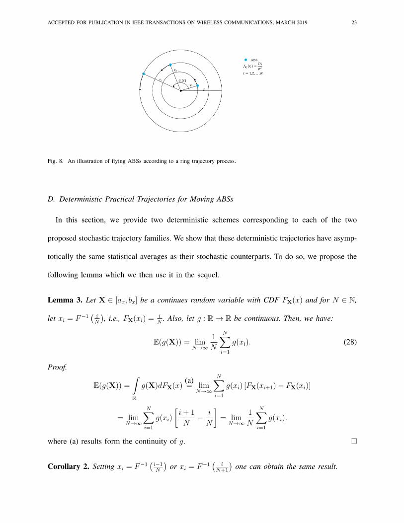
Fig. 8. An illustration of flying ABSs according to a ring trajectory process.

D. Deterministic Practical Trajectories for Moving ABSs

In this section, we provide two deterministic schemes corresponding to each of the two

proposed stochastic trajectory families. We show that these deterministic trajectories have asymp-

totically the same statistical averages as their stochastic counterparts. To do so, we propose the

following lemma which we then use it in the sequel.

Lemma 3. Let X ∈ [ax, bx] be a continues random variable with CDF FX(x) and for N ∈ N,

let xi = F−1(

iN

), i.e., FX(xi) =

iN

. Also, let g : R → R be continuous. Then, we have:

E(g(X)) = limN→∞

1

N

N∑i=1

g(xi). (28)

Proof.

E(g(X)) =

∫R

g(X)dFX(x)(a)= lim

N→∞

N∑i=1

g(xi) [FX(xi+1)− FX(xi)]

= limN→∞

N∑i=1

g(xi)

[i+ 1

N− i

N

]= lim

N→∞

1

N

N∑i=1

g(xi).

where (a) results form the continuity of g.

Corollary 2. Setting xi = F−1(i−1N

)or xi = F−1

(i

N+1

)one can obtain the same result.


θ(rad)0 1 2 3 4 5 6

PD

F0.1

0.11

0.12

0.13

0.14

0.15

0.16

0.17Histogram of Θ

i in deterministic radial trajectory

PDF of Θi in stochastic radial trajectory

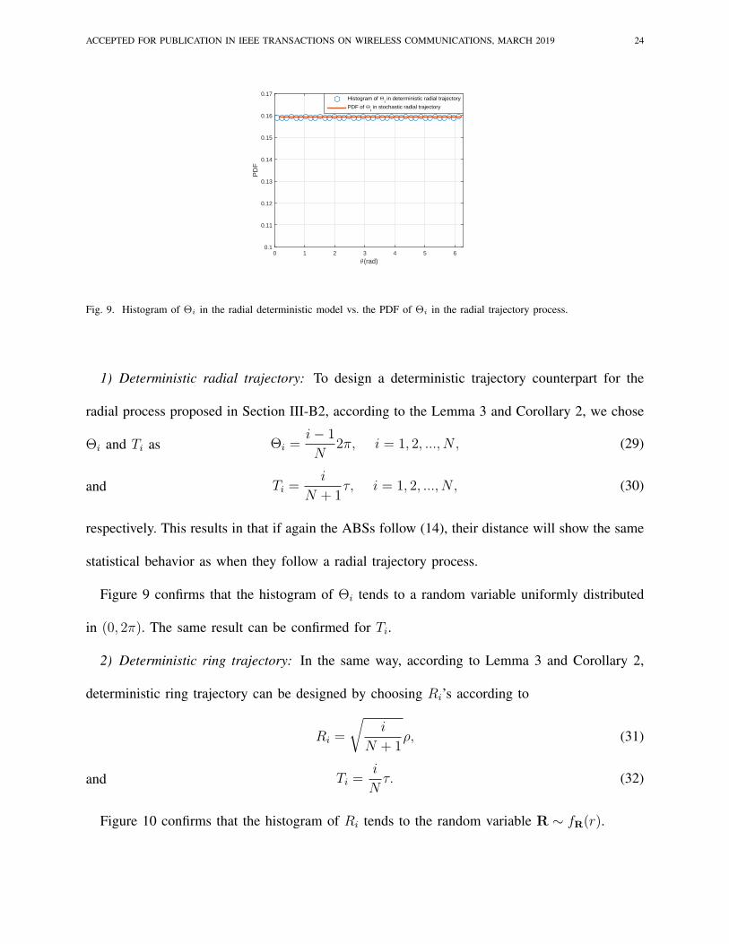
Fig. 9. Histogram of Θi in the radial deterministic model vs. the PDF of Θi in the radial trajectory process.

1) Deterministic radial trajectory: To design a deterministic trajectory counterpart for the

radial process proposed in Section III-B2, according to the Lemma 3 and Corollary 2, we chose

Θi and Ti as Θi =i− 1

N2π, i = 1, 2, ..., N, (29)

and Ti =i

N + 1τ, i = 1, 2, ..., N, (30)

respectively. This results in that if again the ABSs follow (14), their distance will show the same

statistical behavior as when they follow a radial trajectory process.

Figure 9 confirms that the histogram of Θi tends to a random variable uniformly distributed

in (0, 2π). The same result can be confirmed for Ti.

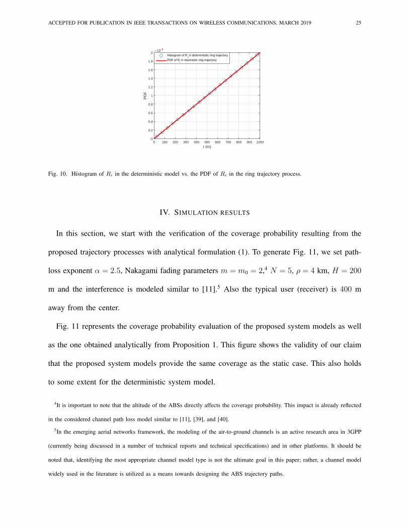
2) Deterministic ring trajectory: In the same way, according to Lemma 3 and Corollary 2,

deterministic ring trajectory can be designed by choosing Ri’s according to

Ri =

√i

N + 1ρ, (31)

and Ti =i

Nτ. (32)

Figure 10 confirms that the histogram of Ri tends to the random variable R ∼ fR(r).


r (m)0 100 200 300 400 500 600 700 800 900 1000

PD

F

×10-3

0

0.2

0.4

0.6

0.8

1

1.2

1.4

1.6

1.8

2Histogram of R

i in deterministic ring trajectory

PDF of Ri in stochastic ring trajectory

Fig. 10. Histogram of Ri in the deterministic model vs. the PDF of Ri in the ring trajectory process.

IV. SIMULATION RESULTS

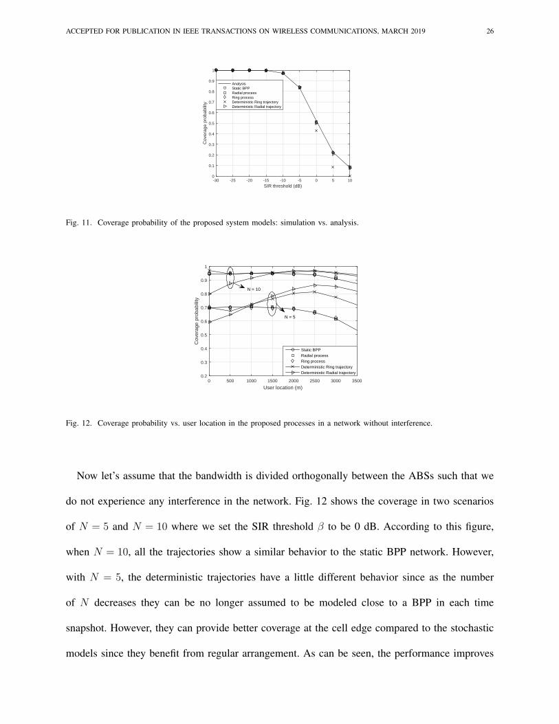
In this section, we start with the verification of the coverage probability resulting from the

proposed trajectory processes with analytical formulation (1). To generate Fig. 11, we set path-

loss exponent α = 2.5, Nakagami fading parameters m = m0 = 2,4 N = 5, ρ = 4 km, H = 200

m and the interference is modeled similar to [11].5 Also the typical user (receiver) is 400 m

away from the center.

Fig. 11 represents the coverage probability evaluation of the proposed system models as well

as the one obtained analytically from Proposition 1. This figure shows the validity of our claim

that the proposed system models provide the same coverage as the static case. This also holds

to some extent for the deterministic system model.

4It is important to note that the altitude of the ABSs directly affects the coverage probability. This impact is already reflected

in the considered channel path loss model similar to [11], [39], and [40].

5In the emerging aerial networks framework, the modeling of the air-to-ground channels is an active research area in 3GPP

(currently being discussed in a number of technical reports and technical specifications) and in other platforms. It should be

noted that, identifying the most appropriate channel model type is not the ultimate goal in this paper; rather, a channel model

widely used in the literature is utilized as a means towards designing the ABS trajectory paths.


SIR threshold (dB)-30 -25 -20 -15 -10 -5 0 5 10

Cov

erag

e pr

obab

ility

0

0.1

0.2

0.3

0.4

0.5

0.6

0.7

0.8

0.9

1

AnalysisStatic BPPRadial processRing processDeterministic Ring trajectoryDeterministic Radial trajectory

Fig. 11. Coverage probability of the proposed system models: simulation vs. analysis.

User location (m)0 500 1000 1500 2000 2500 3000 3500

Cov

erag

e pr

obab

ility

0.2

0.3

0.4

0.5

0.6

0.7

0.8

0.9

1

Static BPPRadial processRing processDeterministic Ring trajectoryDeterministic Radial trajectory

N = 10

N = 5

Fig. 12. Coverage probability vs. user location in the proposed processes in a network without interference.

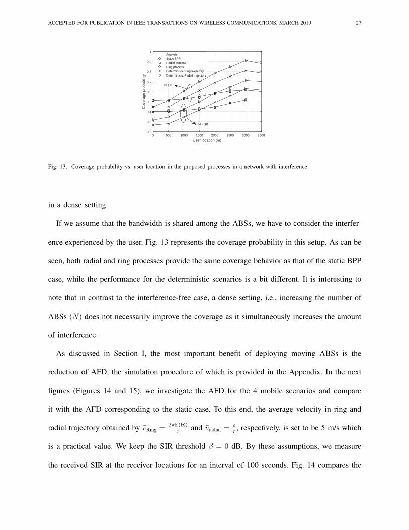
Now let’s assume that the bandwidth is divided orthogonally between the ABSs such that we

do not experience any interference in the network. Fig. 12 shows the coverage in two scenarios

of N = 5 and N = 10 where we set the SIR threshold β to be 0 dB. According to this figure,

when N = 10, all the trajectories show a similar behavior to the static BPP network. However,

with N = 5, the deterministic trajectories have a little different behavior since as the number

of N decreases they can be no longer assumed to be modeled close to a BPP in each time

snapshot. However, they can provide better coverage at the cell edge compared to the stochastic

models since they benefit from regular arrangement. As can be seen, the performance improves


User location (m)0 500 1000 1500 2000 2500 3000 3500

Cov

erag

e pr

obab

ility

0.2

0.3

0.4

0.5

0.6

0.7

0.8

0.9

1AnalysisStatic BPPRadial processRing processDeterministic Ring trajectoryDeterministic Radial trajectory

N = 10

N = 5

Fig. 13. Coverage probability vs. user location in the proposed processes in a network with interference.

in a dense setting.

If we assume that the bandwidth is shared among the ABSs, we have to consider the interfer-

ence experienced by the user. Fig. 13 represents the coverage probability in this setup. As can be

seen, both radial and ring processes provide the same coverage behavior as that of the static BPP

case, while the performance for the deterministic scenarios is a bit different. It is interesting to

note that in contrast to the interference-free case, a dense setting, i.e., increasing the number of

ABSs (N ) does not necessarily improve the coverage as it simultaneously increases the amount

of interference.

As discussed in Section I, the most important benefit of deploying moving ABSs is the

reduction of AFD, the simulation procedure of which is provided in the Appendix. In the next

figures (Figures 14 and 15), we investigate the AFD for the 4 mobile scenarios and compare

it with the AFD corresponding to the static case. To this end, the average velocity in ring and

radial trajectory obtained by vRing =2πE(R)

τand vradial =

ρτ, respectively, is set to be 5 m/s which

is a practical value. We keep the SIR threshold β = 0 dB. By these assumptions, we measure

the received SIR at the receiver locations for an interval of 100 seconds. Fig. 14 compares the


User speed (m/s)0 2 4 6 8 10 12 14 16 18 20

Ave

rage

fade

dua

rion

(s)

10-2

10-1

100

101

102Static BPPRadial processRing processDeterministic radial trajectoryDeterministic ring trajectory

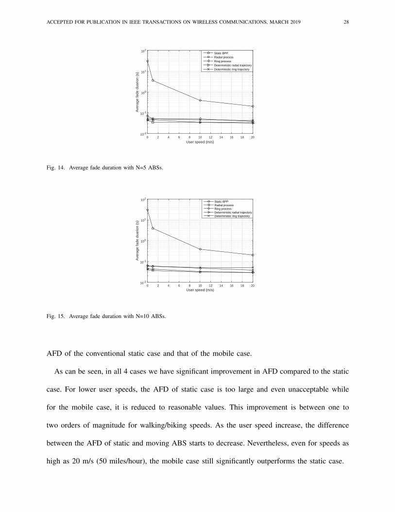
Fig. 14. Average fade duration with N=5 ABSs.

User speed (m/s)0 2 4 6 8 10 12 14 16 18 20

Ave

rage

fade

dua

rion

(s)

10-2

10-1

100

101

102Static BPPRadial processRing processDeterministic radial trajectoryDeterministic ring trajectory

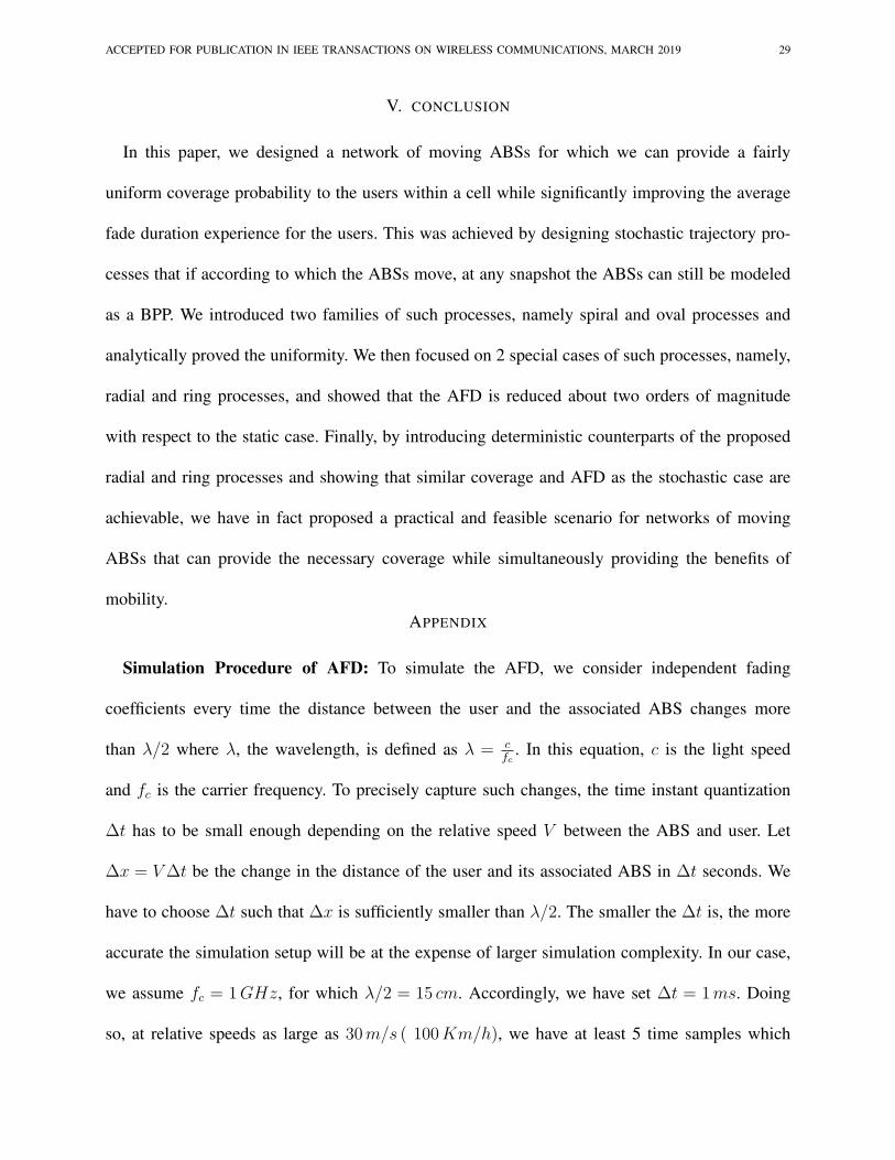
Fig. 15. Average fade duration with N=10 ABSs.

AFD of the conventional static case and that of the mobile case.

As can be seen, in all 4 cases we have significant improvement in AFD compared to the static

case. For lower user speeds, the AFD of static case is too large and even unacceptable while

for the mobile case, it is reduced to reasonable values. This improvement is between one to

two orders of magnitude for walking/biking speeds. As the user speed increase, the difference

between the AFD of static and moving ABS starts to decrease. Nevertheless, even for speeds as

high as 20 m/s (50 miles/hour), the mobile case still significantly outperforms the static case.


V. CONCLUSION

In this paper, we designed a network of moving ABSs for which we can provide a fairly

uniform coverage probability to the users within a cell while significantly improving the average

fade duration experience for the users. This was achieved by designing stochastic trajectory pro-

cesses that if according to which the ABSs move, at any snapshot the ABSs can still be modeled

as a BPP. We introduced two families of such processes, namely spiral and oval processes and

analytically proved the uniformity. We then focused on 2 special cases of such processes, namely,

radial and ring processes, and showed that the AFD is reduced about two orders of magnitude

with respect to the static case. Finally, by introducing deterministic counterparts of the proposed

radial and ring processes and showing that similar coverage and AFD as the stochastic case are

achievable, we have in fact proposed a practical and feasible scenario for networks of moving

ABSs that can provide the necessary coverage while simultaneously providing the benefits of

mobility.APPENDIX

Simulation Procedure of AFD: To simulate the AFD, we consider independent fading

coefficients every time the distance between the user and the associated ABS changes more

than λ/2 where λ, the wavelength, is defined as λ = cfc

. In this equation, c is the light speed

and fc is the carrier frequency. To precisely capture such changes, the time instant quantization

∆t has to be small enough depending on the relative speed V between the ABS and user. Let

∆x = V∆t be the change in the distance of the user and its associated ABS in ∆t seconds. We

have to choose ∆t such that ∆x is sufficiently smaller than λ/2. The smaller the ∆t is, the more

accurate the simulation setup will be at the expense of larger simulation complexity. In our case,

we assume fc = 1GHz, for which λ/2 = 15 cm. Accordingly, we have set ∆t = 1ms. Doing

so, at relative speeds as large as 30m/s ( 100Km/h), we have at least 5 time samples which


observe a fixed fading coefficient. Now we generate the coefficients according the considered

distribution (here, Nakagami) and at each time instant, we record the associated gain for the whole

period of measurement (here T = 100 s) for any user-ABS pair. Now based on the required SIR

threshold, we find blocks of time instants for which all the associated gains are below the given

SIR threshold and record their time length. Then we average over such lengths to obtain the

AFD. To be sure of the accuracy of the chosen ∆t, we have examined smaller values for ∆t

(i.e., 0.1ms) at the expense of increasing the simulation complexity one order of magnitude and

the AFD results were almost the same. Therefore, for the speeds up to 100Km/h, time instants

around 1ms seem to be sufficiently small for simulating AFD.

REFERENCES

[1] S. Enayati, H. Saeedi, and H. Pishro-Nik, “Trajectory processes that preserve uniformity: A stochastic geometry approach,”

Accepted in IEEE International Symposium on Information Theory (ISIT), July 2018, Vail, CO, USA.

[2] N. Goddemeier, K. Daniel, and C. Wietfeld, “Role-based connectivity management with realistic air-to-ground channels

for cooperative UAVs,” IEEE Journal on Selected Areas in Communications, vol. 30, no. 5, pp. 951–963, Jun. 2012.

[3] S. Hayat, E. Yanmaz, and R. Muzaffar, “Survey on unmanned aerial vehicle networks for civil applications: a

communications viewpoint,” IEEE Communications Surveys & Tutorials, vol. 18, no. 4, pp. 2624–2661, 2016.

[4] L. Gupta, R. Jain, and G. Vaszkun, “Survey of important issues in UAV communication networks,” IEEE Communications

Surveys & Tutorials, vol. 18, no. 2, pp. 1123–1152, 2015.

[5] F. Ono, H. Ochiai, and R. Miura, “A wireless relay network based on unmanned aircraft system with rate optimization,”

IEEE Transactions on Wireless Communications, vol. 15, no. 11, pp. 7699–7708, Nov. 2016.

[6] Y. Zeng and R. Zhang, “Energy-efficient UAV communication with trajectory optimization,” IEEE Transactions on Wireless

Communications, vol. 16, no. 6, pp. 3747–3760, Jun. 2017.

[7] A. Filippone, Flight Performance of Fixed and Rotary Wing Aircraft. American Institute of Aeronautics & Ast., 2006.

[8] M. Guizani, Wireless Communications Systems and Networks. Kluwer Academic Publishers, 2004.

[9] M. Mozaffari, W. Saad, M. Bennis, and M. Debbah, “Unmanned aerial vehicle with underlaid device-to-device communi-

cations: Performance and tradeoffs,” IEEE Transactions on Wireless Communications, vol. 15, no. 6, pp. 3949–3963, Jun.

2016.


[10] J. Lyu, Y. Zeng, and R. Zhang, “Cyclical multiple access in UAV-aided communications: A throughput-delay tradeoff,”

IEEE Wireless Communications Letters, vol. 5, no. 6, pp. 600–603, Dec. 2016.

[11] V. V. Chetlur and H. S. Dhillon, “Downlink coverage analysis for a finite 3D wireless network of unmanned aerial vehicles,”

IEEE Transactions on Communications, vol. 65, no. 10, pp. 4543–4558, Oct. 2017.

[12] Y. Zeng, R. Zhang, and T. J. Lim, “Throughput maximization for UAV-enabled mobile relaying systems,” IEEE Transactions

on Communications, vol. 64, no. 12, pp. 4983–4996, Dec. 2016.

[13] C. Zhang and W. Zhang, “Spectrum sharing for drone networks,” IEEE Journal on Selected Areas in Communications,

vol. 35, no. 1, pp. 136–144, Jan. 2017.

[14] M. Mozaffari, W. Saad, M. Bennis, and M. Debbah, “Drone small cells in the clouds: Design, deployment and performance

analysis,” in IEEE Global Communications Conference (GLOBECOM), San Diego, CA, USA, Dec. 2015, pp. 1–6.

[15] J. Lyu, Y. Zeng, R. Zhang, and T. J. Lim, “Placement optimization of UAV-mounted mobile base stations,” IEEE

Communications Letters, vol. 21, no. 3, pp. 604–607, Mar. 2017.

[16] E. Kalantari, H. Yanikomeroglu, and A. Yongacoglu, “On the number and 3D placement of drone base stations in wireless

cellular networks,” in Proc. of IEEE Vehicular Technology Conference (VTC-Fall), Montreal, QC, Canada, Sep. 2016.

[17] M. Mozaffari, W. Saad, M. Bennis, and M. Debbah, “Efficient deployment of multiple unmanned aerial vehicles for optimal

wireless coverage,” IEEE Communications Letters, vol. 20, no. 8, pp. 1647–1650, Aug. 2016.

[18] ——, “Optimal transport theory for power-efficient deployment of unmanned aerial vehicles,” in Proc. of IEEE International

Conference on Communications, Kuala Lumpur, Malaysia, May 2016, pp. 1–6.

[19] ——, “Optimal transport theory for cell association in UAV-enabled cellular networks,” IEEE Communications Letters,

vol. 21, no. 9, pp. 2053–2056, Sep. 2017.

[20] R. Yaliniz, A. El-Keyi, and H. Yanikomeroglu, “Efficient 3-D placement of an aerial base station in next generation cellular

networks,” in Proc. of IEEE International Conference on Communications, Kuala Lumpur, Malaysia, May 2016, pp. 1–5.

[21] M. Mozaffari, W. Saad, M. Bennis, and M. Debbah, “Mobile unmanned aerial vehicles (UAVs) for energy-efficient internet

of things communications,” IEEE Transactions on Communications, vol. 16, no. 11, pp. 7574–7589, Nov. 2017.

[22] Q. Wu, Y. Zeng, and R. Zhang, “Joint trajectory and communication design for uav-enabled multiple access,” in IEEE

Global Communications Conference (GLOBECOM). IEEE, Singapore, Singapore, Dec. 2017, pp. 1–6.

[23] ——, “Joint trajectory and communication design for multi-UAV enabled wireless networks,” IEEE Transactions on

Wireless Communications, vol. 17, no. 3, pp. 2109–2121, March 2018.

[24] J. Lyu, Y. Zeng, and R. Zhang, “UAV-aided offloading for cellular hotspot,” IEEE Transactions on Wireless Communica-

tions, vol. 17, no. 6, pp. 3988 – 4001, Jun. 2018.

[25] W. Feng, J. Wang, Y. Chen, X. Wang, N. Ge, and J. Lu, “UAV-aided MIMO communications for 5G internet of things,”


IEEE Internet of Things Journal, Early Access 2018.

[26] B. Galkin, J. Kibilda, and L. A. DaSilva, “A stochastic geometry model of backhaul and user coverage in urban UAV

networks,” arXiv preprint arXiv:1710.03701, 2017.

[27] Y. Cai, F. Cui, Q. Shi, M. Zhao, and G. Li, “Dual-UAV enabled secure communications: joint trajectory design and user

scheduling,” IEEE Journal on Selected Areas in Communications, vol. 36, no. 9, pp. 1972 – 1985, Sep. 2018.

[28] Q. Wang, Z. Chen, H. Li, and S. Li, “Joint power and trajectory design for physical-layer secrecy in the UAV-aided mobile

relaying system,” IEEE Access, vol. 6, pp. 62 849–62 855, 2018.

[29] X. Jiang, Z. Wu, Z. Yin, and Z. Yang, “Joint power and trajectory design for UAV-relayed wireless systems,” IEEE Wireless

Communications Letters, Early Access, 2018.

[30] L. Xie, J. Xu, and R. Zhang, “Throughput maximization for UAV-enabled wireless powered communication networks,”

IEEE Internet of Things Journal, Early Access, 2018.

[31] X. Zhou, S. Yan, J. Hu, J. Sun, J. Li, and F. Shu, “Joint optimization of a UAVs trajectory and transmit power for covert

communications,” arXiv preprint arXiv:1812.00583, Dec. 2018.

[32] Y. Zeng, X. Xu, and R. Zhang, “Trajectory design for completion time minimization in UAV-enabled multicasting,” IEEE

Transactions on Wireless Communications, vol. 17, no. 4, pp. 2233–2246, Apr. 2018.

[33] G. Zhang, H. Yan, Y. Zeng, M. Cui, and Y. Liu, “Trajectory optimization and power allocation for multi-hop UAV relaying

communications,” IEEE Access, vol. 6, pp. 48 566–48 576, Aug. 2018.

[34] S. Eom, H. Lee, J. Park, and I. Lee, “UAV-aided wireless communication designs with propulsion energy limitations,”

arXiv preprint arXiv:1801.02782, 2018.

[35] M. Haenggi, J. G. Andrews, F. Baccelli, O. Dousse, and M. Franceschetti, “Stochastic geometry and random graphs for

the analysis and design of wireless networks,” IEEE Journal on Selected Areas in Communications, vol. 27, no. 7, Sep.

2009.

[36] J. G. Andrews, A. K. Gupta, and H. S. Dhillon, “A primer on cellular network analysis using stochastic geometry,” arXiv

preprint arXiv:1604.03183, 2016.

[37] H. ElSawy, A. Sultan-Salem, M.-S. Alouini, and M. Z. Win, “Modeling and analysis of cellular networks using stochastic

geometry: A tutorial,” IEEE Communications Surveys & Tutorials, vol. 19, no. 1, pp. 167–203, Firstquarter 2017.

[38] M. Haenggi, Stochastic Geometry for Wireless Networks. Cambridge University Press, 2012.

[39] I. Atzeni, J. Arnau, and M. Kountouris, “Downlink cellular network analysis with los/nlos propagation and elevated base

stations,” IEEE Transactions on Wireless Communications, vol. 17, no. 1, pp. 142–156, Jan. 2018.

[40] Y. Zhu, G. Zheng, and M. Fitch, “Secrecy rate analysis of UAV-enabled mmwave networks using matern hardcore point

processes,” IEEE Journal on Selected Areas in Communications, vol. 36, no. 7, pp. 1397 – 1409, Jul. 2018.

Documents

Moving Aerial Base Station Networks: Stochastic Geometry ...Moving Aerial Base Station Networks: Stochastic Geometry Analysis and Design Perspective S. Enayati, H. Saeedi, H. Pishro-Nik,