Moving from Customer Lifetime Value to Customer Equity

Xavier Drèze

André Bonfrer*

September 2005

* Xavier Drèze is Assistant Professor of Marketing at the Wharton School of the University of Pennsylvania, 3730 Walnut street, Philadelphia, PA 19104-6340, 215-898-1223, Fax 215-898-2534, xdreze@wharton.upenn.edu. André Bonfrer is Assistant Professor of Marketing at the Lee Kong Chian School of Business, Singapore Management University. This research was funded in part by the Wharton-SMU research center, Singapore Management University and in part by a WeBI - Mac Center Grant.

Moving from Customer Lifetime Value to Customer Equity

Abstract

We study the consequence of moving from Customer Lifetime Value maximization to Customer Equity

maximization. Customer equity has traditionally been seen as the discounted sum of the lifetime value of

all current and future customers and thus it has been largely assumed that maximizing customer lifetime

value would lead to maximum customer equity. We show that the transition from CLV to CE is not that

straightforward. Although the CLV model is appropriate for managing a single non-replaceable customer,

the application of a CLV model to the valuation of customers when an acquisition process is in place leads

to sub-optimal customer relationship management and acquisition strategies. We also derive a simple

solution to the customer equity optimization problem.

Keywords: Customer Equity, Database Marketing, Customer Lifetime Value, Internet Marketing,

Direct Marketing, Customer Acquisition

1 Introduction

There has been a recent move towards using Customer Equity as a marketing metric both for assessing the

return of marketing actions and to value firms as a whole. The metric, proposed by Blattberg and

Deighton (1996) and defined by Rust, Lemon, and Zeithaml (2004) as “the total of the discounted lifetime

values summed over all the firm’s current and potential customers,” seeks to asses the value of not only a

firm’s current customer base, but also its potential or future customer base as well. This long term view

seems appropriate since a firm’s actions at any given time do not only affect its customer base at that

point in time, but they also affect its ability to recruit and retain customers in subsequent time periods.

Customer Equity (CE) has been endorsed by many researchers. For instance, Berger et al (2002)

make CE the foundation on which they build their framework for managing customers as assets; Bayon,

Gutsche, and Bauer (2002) make a case that CE is the best basis for customer analysis; Gupta, Lehmann,

and Stuart (2004) use CE as a basis for valuing firms.

At the core of CE is the Customer Lifetime Value (CLV). The CLV metric is an adaptation of the

concept of discounted cash flow or net present value from financial analysis. It seeks to compute the

value of a customer by discounting the future revenues expected from the customer to the present. It is

constructed using core metrics such as customer retention rate, revenue per customer, and discount rate of

money. Berger and Nasr (1998) discuss the concept in detail and provide many different ways to

compute it depending on the situation the firm is facing.

When building CE as the aggregation of current and future customers’ CLV, researchers have

taken for granted that the precepts coming out of a CLV analysis still apply when looking a Customer

Equity. For instance, a common belief is that if one spends more on acquiring a customer than his/her

CLV then one loses money. Another is that what maximizes the CLV will also maximize the CE.

While there is no doubt that the CLV concept is what it claims to be, the value in present terms of

future earnings from a given customer, we question whether it is still an appropriate metric when one

considers the larger and long term goal of the firm to maximize its customer equity. Can CLV still be

used to evaluate and optimize marketing actions? Does a firm that maximizes the CLV for a group of

2

customers maximize its Customer Equity? Is the CLV the proper benchmark when setting a customer

acquisition policy? If not, what is the appropriate metric? How can the firm compute it? How can the

firm adjust its marketing actions to optimize it?

We answer these questions in the remainder of this paper. We start with a discussion of

customers as a resource to the firm (section 2.1) and how the firm should aim to maximize the long-term

value of this resource. Based on this discussion, we derive a general functional form for a firm’s

Customer Equity in section 2.3. In sections Error! Reference source not found. and 4, we derive the

first order condition that must be satisfied to maximize CE and perform comparative statics to show how

marketing actions should be adapted when control variables (e.g., retention rate, acquisition effectiveness)

change. We show how maximizing CE is different from maximizing CLV such that maximizing CLV is

sub-optimal from a customer equity standpoint. Then, in section 5, we discuss the impact of a long term

focus on acquisition spending. We show that firms that aim to maximize CE should be more aggressive

in their acquisition policy than is predicated by CLV proponents. In section 6, we show our model to be

robust to both observed and un-observed heterogeneity. We conclude the paper in section 7.

2 A Customer Equity Model

For modeling purposes, and in the spirit of Berger et al (2002), we consider the case of a firm that is

trying to generate revenues by contacting members of its database. Customers are recruited through an

acquisition policy and are contacted at fixed intervals. The problem of the firm is to find the marketing

actions, defined as the acquisition spending and contact periodicity, that will maximize its expected

revenues, taking into account the various costs it faces (acquisition, communication) and the reaction of

customers to the firm’s policy (defection, purchase).

When developing a model of customer equity, we pay particular attention to two processes. First,

we seek to capture the customer acquisition/retention process in a meaningful way. Second, we seek to

capture the impact of the firm’s marketing actions on customer retention and expenditure.

3

2.1 Customer flow: acquisition and retention process

Fundamentally, managing a database of customer names hinges on balancing the retention of the

customer and the ability of the marketer to continue to extract rents from its current list of customers. The

problem of extracting the highest possible profits from a database of customer names is similar to the

challenges encountered by researchers studying the management of natural resources. Economists

(Sweeny 1992) consider three types of resources: depletable, renewable, and expendable. The distinction

is made based on the time scale of the replenishment process. Depletable resources, such as crude oil

reserves, are those whose replenishment process is so slow that one can model them as being available

once and only once. Renewable resources, such as the stock of fish in a lake or pond, adjust more rapidly

so that they renew within the time horizon studied. However, any action in a given time period that alters

the stock of the resource will have an impact on the subsequent periods. Finally, expendable resources,

such as solar energy, renew themselves at such a speed that their use in one period has little or no impact

on subsequent periods.

Depending on the type of resource a firm is managing, it faces a different objective. In the case of

a depletable resource, the firm is interested in the optimal use of the resource in its path to depletion. With

a renewable resource, the firm is interested in long-term equilibrium strategies. Faced with an expendable

resource, the firm is interested in its best short-term allocation.

When looking at its customer database, a firm can treat its customers as any of these three

resource types depending on the lens it uses for the problem. In the cohort view (the basis for CLV),

customers are seen as a depletable resource. New cohorts are recruited over time, but each cohort will

eventually become extinct (see Wang and Spiegel 1994). Attrition is measured by the difference in cohort

size from one year to another. In an email-SPAM environment, where consumers cannot prevent the firm

from sending them emails, and where new email names can readily be found by “scrubbing” the Internet,

the firm views consumers as an expendable resource and thus can take a short-term approach to profit

maximization.

4

Customer equity takes a long term approach to valuing and optimizing a firm’s customer base.

For a firm with a long-term horizon, a depletable resource view of customers is not viable as it implies

that the firm will lose all its customers at some point. Thus a customer acquisition process must be in

place for the firm to survive. Further, if the firm observes defection and incurs acquisition costs to replace

lost customers, then it cannot treat its customers as expendable. Hence, we argue that the appropriate way

to look at the profit maximization problem is to view customers as a renewable resource. This view is the

basis for our formulation and analysis of a firm’s customer equity. Further, if the firm views customers as

a renewable resource, then it must evaluate its policies in terms of the long-term equilibrium they

generate. This is the approach we take in this paper.

2.2 The Impact of marketing actions on customer retention and expenditure

One cannot capture in a simple model the impact of all possible marketing actions (pricing decisions,

package design, advertising content…). Hence, as in Venkatesan and Kumar (2004), we concentrate on

optimizing the frequency with which a firm should contact its customer base. It is a broadly applicable

problem that is meaningful for many applications, not only for the timing of mail or email

communications, but also the frequency of calls by direct sales force or the intensity of broadcast

advertising. It is also a more interesting process to model than some of the other natural candidates. For

instance, the impact of marketing communication content on customer attrition is straightforward. Poor

content leads to lower retention rates and smaller revenues than good content. In contrast, the effect of the

periodicity of communication on attrition is more pernicious. To see why, one can conduct the following

thought experiment: let us consider the two extremes in contact periodicity. At one extreme, a firm might

contact its clients so often that the relationship becomes too onerous for the clients to maintain and thus

they sever their links to the company, rendering their names worthless. (Evidence of this phenomenon can

be seen in the emergence of the ‘Do Not Call Registry’ in 2003 as well as the Anti-Spamming Act of

2001.) At the other extreme, the firm never contacts its customers and, although the names have a

potential value, this value is never realized. Thus, periodicity affects the value of names in two ways. On

the one hand, more frequent contact leads to more opportunities to earn money. On the other hand, more

5

frequent contacts provide customers with more opportunities to defect. The latter can quickly lead to high

long-term attrition. Imagine the case of a company that has a retention rate of 97% from one campaign to

another. This might at first glance seem like outstanding loyalty. However, if the firm were to contact its

database every week, and ignoring the acquisition of new names, it would lose 80% of its customers

within a year! Clearly, there must be an intermediary situation where one maximizes the realized value

from a name by optimally trading off the extraction of value in the short-term against the loss of future

value due to customer defection.

2.3 Customer Equity

Our customer equity model is in essence a version of the model developed by Gupta et al (2004) that has

been modified to directly take into account the requirement described in the preceding two sections. In

particular, we explicitly develop a consumer production function ( ( )iS τ ) that characterizes how the

customer base evolves from one period to another as a function of acquisition and retention. We also

make customer retention and customer spending a function of the time elapsed between communication

(τ ).

Because the time elapsed between each communication is a control variable, we must be careful

when discounting revenues and expenses. To apply the correct discount rate to expenses and revenues,

one must pinpoint when each occurs. Consistent with Venkatesan and Kumar (2004), we assume that

acquisition expenses are an ongoing expenditure that the firm recognizes on a periodic basis (e.g.,

monthly) while communications expenses and revenues are recognized at the time of the communication.

This assumption is also consistent with our observations of practice, where the acquisition costs are

decoupled from the marketing activities once the names are acquired. This is also a recommendation of

Blattberg and Deighton (1996), highlighting the different roles of acquisition and retention efforts.

Based on these assumptions, Customer Equity can be generally defined as:

( )0 0

( ) ( ) ( )ir jri i i

i jCE e R S FC e AQττ τ τ

∞ ∞−

= =

= − −∑ j−∑ . (1)

6

Where:

i is an index of communications,

j is an index of time periods,

re− is the per period discount rate1,

τ is the periodicity of contact,

( )iR τ is the expected profit (revenues net of cost of goods sold and variable communication

costs) per customer for communication i ,

( )iS τ is the number of people in the database when communication i was sent,

iFC is the fixed cost associated with communication i ,

jAQ is the acquisition costs incurred in time period . j

Further, we define the customer profit ( ( )iR τ ) and production ( ( )iS τ ) functions as:

(( ) ( )i iR A VCτ τ= − )i (2)

1( ) ( ) ( ) ( )i i i iS S P gτ τ τ τ−= + (3)

Where:

( )iA τ is the expected per-customer gross profit for communication , i

iVC is the variable cost of sending communication i ,

0 ( ) 0S τ = ,

( )iP τ is the retention rate for communication i ,

( )ig τ is the number of names acquired between campaigns 1i − and i .

The model laid out above is a general case that is applicable in any situations. However, we make

the following simplifications in order to make the maximization problem more tractable. First, we

assume that the acquisition efforts are constant over time and produce a steady stream of names (i.e.,

7

( ) .ig gτ τ= , ( )jAQ AQ g= ). There is no free production of names and the cost of acquisition increases

with the size of the name stream such that: (0) 0AQ = , . Second, we assume that the fixed

and variable communications costs are constant across communications (i.e., , ).

Third, we assume that the communications are identical in nature, if not in actual content, and that

customers’ reaction to the communications depends only on their frequency such that:

( ) ' 0AQ g >

iVC VC= iFC FC=

( ) ( )iA Aτ τ= 2 and

( ) ( )iP Pτ τ= . Further, we assume that ( )A τ is monotonically increasing in τ , with and

finite (i.e., the more time the firm has to come up with a new offer, the more attractive it can make

it –up to a point), and that

(0) 0A =

( )A ∞

( )P τ is inverted-U shaped (i.e., retention is lowest when the firm sends

incessant messages or when it never contacts its customers and there is a unique optimal communication

periodicity for retention purposes) and dependent on ( )A τ such that ( ) / ( ) 0P Aτ τ∂ ∂ > (i.e., the better

the offer, the higher the retention rate).

We assume that customers are treated by the firm as homogenous entities; there is no observed

heterogeneity the firm can use to derive different τ for different individual. We feel justified in doing so

by the recommendation of researchers (Zeithaml, Rust, and Lemon 2001, Berger et al 2002, Libai,

Narayandas, and Humby 2002, Hwang, Jung, and Suh 2004), which is widely followed in practice, that

customers be segmented in fairly homogenous groups and that each group be treated independently. With

this in mind, we would argue that each customer segment has its own CE with its own acquisition and

retention process; equation (1) can be applied to each of these segments. Nevertheless, we will discuss

heterogeneity issues in section 6.

We defer to the technical appendix for a more complete justification of our assumptions. We also

discuss the robustness of the major findings to the relaxation of these assumptions later in this paper when

appropriate. Building on these assumptions, we can rewrite the customer equity equations as follows:

( )0 0

( ) ( ) ( ) ( )ir jri

i jCE e R S FC e AQ gττ τ τ

∞ ∞−

= =

= − −∑ ∑ − (4)

8

1( ) ( ) ( ) .i iS S P gτ τ τ τ−= +

)

(5)

(( ) ( ) .R A VCτ τ= − (6)

We show (Lemma 1) that, given (5), in the long run, the database reaches an equilibrium size,

regardless of the number of names the firm is endowed with at time 0 ( ): 0S

Lemma 1: For any given constant marketing actions there exists a steady state such that the

database is constant in size. The steady state size is .

1 (gS

P )τ

τ=

−.

Proof: See Appendix A.1.

The intuition behind Lemma 1 is straightforward given the database production function (5). For any

given τ the firm acquires a constant number of new names ( .gτ ) between every communication, but it

loses names in proportion ( ( )P τ ) to its database size. Consequently, the database will be at equilibrium

when the firm, between one communication and the next, acquires as many names as it loses due to the

communication.

This is analogous to Little’s Law, which states that an inventory reaches a steady state size, L,

which is a product of the arrival rate of new stock (λ ) and the expected time spent by any single unit of

stock in the inventory (W ) or L Wλ= (Little 1961). When Little’s Law is applied to an inventory of

customer names we have L S= the expected number of units in the system, .gλ τ= the arrival rate of

new units, and W 1/(1 ( ))P τ= − the expected time spent by a unit in the system. Little’s Law yields a

finite inventory size, as long as λ and W are both finite and stationary. This law has been the subject of

numerous papers and has been shown to hold under very general assumptions. This means that Lemma 1

will hold (in expected value) for any stochastic acquisition and retention process as long as they are

stationary in the long run, that τ and g are finite, and ( ) 1P τ < . The appeal of Little’s Law applied to

the CE problem is its robustness - this relationship holds even if:

9

• there is seasonality in retention or acquisition (aggregated to the year level, these processes

become stationary – e.g., g = E[Yearly acquisition rate]),

• the firm improves its ability to attract new customers (as long as lim ( )t

g g→∞

t= is finite, where t is

the length of time the firm has been in business),

• there is heterogeneity in customer retention (see Section 6),

• customer retention probability increases–possibly due to habit formation or inertia–as customers

stay in the database longer (provided that lim ( , ) 1t

P tτ→∞

< , where t is the length of time during

which a customer has been active).

In section 6.3 we use a simulation to illustrate this stationarity property of Lemma 1.

Lemma 1 yields some interesting properties for the CE model. First, it allows managers to ex ante

predict the long-term database size and CE. All they need to know is their long-term attrition rate and

acquisition effectiveness. This is particularly important when valuating young companies (e.g., start-ups)

as it provides a monitoring tool and a base for predicting long-term value. Second, it allows us to further

simplify the formulation of CE. Indeed, we can write the steady state CE:

( )0 0

( ) ( ) ( ) ( )ir jr

i jCE e R S FC e AQ gττ τ τ

∞ ∞− −

= =

= − −∑ ∑ ,

or, taking the limit of sums:

( )( ) ( ) ( ) ( ) .1 1

r r

r

e eCE R S FC AQ ge e

τ

ττ τ τ= − − r− − (7)

Third, the elements of (7) are quite easy to compute for database marketers. Having a database of

names they track, they can measure S (it is the number of live names in the database), they can compute

R as the average per-customer profit per campaign, the various costs can be obtained from their

accounting department (as is r). Finally, they can set τ to maximize ( )CE τ as discussed in Proposition

2, below.

10

Fourth, the optimal marketing actions and the resulting steady state database size is a function of

the rate of the acquisition stream, not its cost. We formalize this point in Lemma 2.

Lemma 2: Given an acquisition stream, the marketing actions that maximize CE depend on

the rate of acquisition, but are separable from the cost of acquisition.

Proof: The proof is straightforward. One only needs to recognize that CE can be split in

two terms. The first one depends on g and τ , the second one depends on g only. That is:

( )( ) ( ),

( ) ( ) ( ) ( )1 1

r r

r r

k gf g

e eCE R S FC AQ ge e

τ

τ

τ

τ τ τ= − −− −

.

Further, to maximize CE with respect to τ one computes ( ) /CE τ τ∂ ∂ such that:

( ) ( )( ) , ( ) ,CE f g k g f g 0.τ τ ττ τ τ τ

∂ ∂ ∂ ∂= − =

∂ ∂ ∂ ∂=

The essence of the proof stems from the observation that the acquisition expenditures precede and

are separable from the frequency of contact or the message content. Once names have entered the

database, it is the marketer’s responsibility to maximize the expected profits extracted from those names,

with the consideration that the cost of acquisition is a sunk cost. That is, when optimizing the contact

strategy, the firm only needs to know how many new names are acquired every month, not how much

these names cost. Everything else being constant, two firms having the same acquisition rate, but different

acquisition costs will have identical inter-communication intervals (but different overall profitability).

Lemma 2 belies the belief that one should be more careful with names that were expensive to

acquire than with names that were acquired at low cost. This does not imply, however, that acquisition

costs are irrelevant. The long-term profitability of the firm relies on the revenues generated from the

database being larger than the acquisition costs. Further, acquisition costs are likely to be positively

correlated with the quality of the names acquired (where better quality is defined by either higher

retention or higher revenue per customer). Nevertheless, the optimal marketing activity are a function of

11

the acquisition rate (g) and can be set without knowledge of the cost associated with this acquisition rate

(AQ(g)).

The importance of Lemma 2 is that it allows us to split customer equity in two part: the value of

the customer database and the cost of replenishing the database to compensate attrition. We can thus

study the optimization problem in two stages. First, solve (Section 3.1) the problem of maximizing the

database value given a predetermined acquisition stream (i.e., find ). Second, optimize (Section * | gτ 5)

the acquisition spending given the characterization of *τ . Further, this Lemma formalizes Blattberg and

Deighton’s (1996) suggestion that, when maximizing customer equity, the “acquisition” and the

“customer equity” management tasks are very different, and should be treated separately.

3 Customer Equity and Customer Lifetime Value

We now turn to the profit maximization problem given an acquisition stream of names (g). As we have

shown in the previous section, if the acquisition expenditures are independent of τ , we can ignore them

when optimizing the communication strategy. The problem to the firm then becomes:

( )0

( ) ( ) ( ) .max1

r

ce r

eV R S FCe

τ

ττ

τ τ τ>

= −−

(8)

where V (the database value part of CE) represents the net present value of all future expected

profits and the subscript ce indicates that we take a customer equity approach, as opposed to the customer

lifetime value approach that we will formulate shortly (using clv as a subscript). We show in Proposition

1 that maximizing the CLV leads to different solutions than maximizing Vce such that maximizing the

CLV is sub-optimal with regard to long-term customer equity maximization.

Proposition 1: CLV maximization is sub-optimal with regard to the long-term profitability of the

firm.

Proof: See Appendix A.2.

12

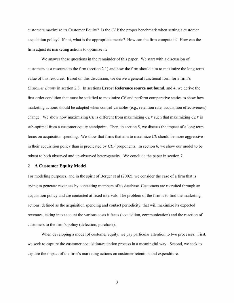
When computing a CLV one accounts for the fact that, due to attrition, customers have a decreasing

probability of being active as time passes. Given our notation, one would write the CLV of an individual

customer as:

0( ) ( ) ( )

( ) .( )

ir i

i

r

r

FCCLV e P RS

FC eRS e P

τ

τ

τ

τ τ τ

ττ

∞−

=

⎛ ⎞= −⎜ ⎟⎝ ⎠

⎛ ⎞= −⎜ ⎟ −⎝ ⎠

∑

(9)

Thus, we can restate the database value (8) in terms of the customer lifetime value as:

( )( ) ( ) .1

r

ce r

e PV CLV Se

τ

τ

ττ τ −=

− (10)

In this equation, the multiplier ( ) 11

r

r

e Pe

τ

τ

τ−>

− accounts for the fact that customers are renewable

and lost customers are replaced. The lower the retention rate, the higher the multiplier. Further, the

multiplier increases as the discount rate (r) or the communication interval (τ) decreases. One can see

evidence of this multiplier at play in the results produced by Gupta et al (2004). Indeed, although they do

consider some future customer acquisition, their model assumes that “as a firm reaches maturity and its

customer acquisition slows, it will eventually lose all its customers.” Although their model is an

improvement on the straight CLV approach, it still undervalues future revenues. Looking at their results,

we can compute the correlation between their assumed retention rate and the ratio of their estimated

customer value (an enhanced CLV estimate) to the book value of the firm (see table 4 in their paper). Per

equation (10) we would expect a negative correlation. We find the correlation (based on the five firms

studied) between the assumed retention rate and the customer value metric to book value ratio to be -0.80

(p = .1).

Following equation (10), the database value is equal to the CLV multiplied by a correction factor.

Maximizing the CLV will thus lead to the maximum customer equity if and only if, at the maximum CLV,

the derivative of the multiplier with respect to τ is equal to 0. We show in Appendix A.2 that this can

13

only occur if . But, as we will show in the next section, * 0τ = *τ is always strictly greater than zero.

Thus, the marketing actions that maximize the CLV do not also maximize the long term CE of the firm.

Therefore, CLV maximization is sub-optimal for the firm!

One should note that when computing the CLV (9) we allocated a portion of the campaign costs

(FC) to each name. This allocation does not affect the substance of our findings. Indeed, if we were to

ignore the fixed costs at the name level, we would compute the CLV as:

( ) ( )( )

r

r

eCLV Re P

τ

ττ ττ

=−

. (11)

Thus, we would have:

( )( ) ( )1 1

r r

ce r r

e P eV CLV S FCe e

τ τ

τ τ

ττ τ −⎡ ⎤= −⎣ ⎦ − −.

The value of the database as a whole is the value of its names minus the costs associated with extracting

profits from these names. In valuating each name we find the same multiplier ( )1

r

r

e Pe

τ

τ

τ⎛ ⎞−⎜ −⎝ ⎠

⎟ as we had

when we incorporated the costs directly in the name value.

3.1 Finding the optimal periodicity ( *τ )

In order to optimize the firm’s marketing actions for any given acquisition strategy, we calculate the first-

order condition for optimality by differentiating (8) with respect to τ . Without further specifying the

general functions that constitute the database value, it is not possible to generate an explicit closed-form

solution for optimal τ . However, for our purposes, we can make some inferences using comparative

static tools. We start by describing the first-order condition, expressed as a function of the elasticities of

the retention and profit functions with respect to changes in the inter-communication interval. Then, we

study how the first-order condition changes with respect to retention rates, profit functions, acquisition

rates, and discount rates.

14

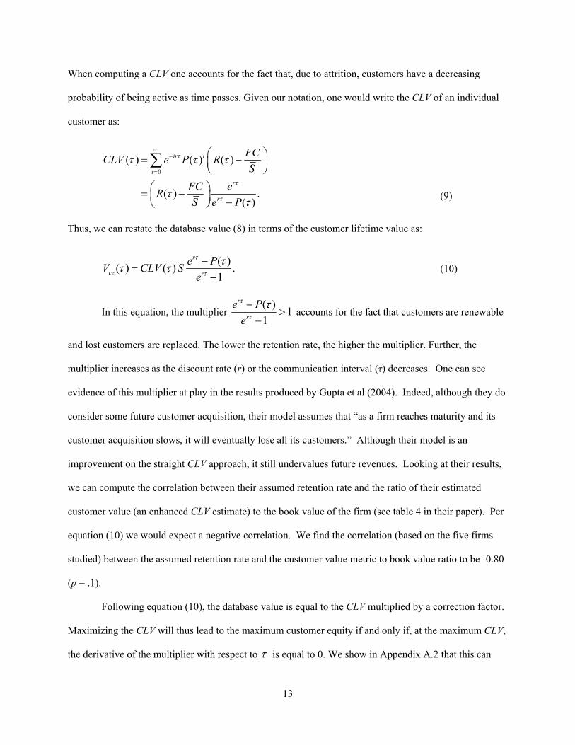
Proposition 2: The first-order condition for a firm that seeks to maximize its database value by

optimizing the inter-communication interval is:

. 0R DS GMη η η+ + = . (12)

Where:

( ) ( )( ) ( )R

R AR A VC

τ τ τ τητ τ τ τ

∂ ∂= =

∂ ∂ − is the elasticity of ( )R τ with respect to τ ,

( )11 ( )S

PP

τ τητ τ

∂= +

∂ − is the elasticity of S with respect to τ ,

1D r

re τ

τη −=

− is the elasticity of the discount multiplier ( )

1

r

r

eDe

τ

ττ⎛ ⎞

=⎜ ⎟−⎝ ⎠ with respect to τ ,

( ). ( )( ). ( )

R S FCGMR Sτ τ

τ τ−

= is the gross margin yielded by each communication.

Proof: See Appendix B.1.

The proof of Proposition 2 is an algebraic exercise that leads to a simple expression of the first-order

condition: a linear combination of elasticities. The optimal inter-communication interval ( *τ ) is found

when the sum of elasticities is equal to 0. When the sum is positive, the firm would increase its value by

increasing τ . When the sum is negative, the firm would be better off decreasing its τ . As we show in the

Technical Appendix, if there exists a τ such that ( )ceV τ is positive, then there exists a unique *τ that is

finite and strictly positive. This is not a restrictive condition, as it only assumes that it is possible for the

firm to make some profits. If it were not the case, the firm should not pursue database driven marketing

and the search for an optimal τ becomes meaningless. Further, if ( )P τ is not too convex then there are

no local maxima and thus the maximum is unique. This, again, is not restrictive, as ( )P τ will typically

be concave over the domain of interest.

15

4 The Impact of Retention rate, Discounts, Revenues and Acquisition rates on Customer

Equity

Our framework for the valuation of customer equity relies on several metrics commonly used to

characterize a customer database: retention rate, acquisition rate, customer margins (revenues and costs),

and discount rates. When any of these change, the marketing action (τ ) must change to reach the new

maximum customer equity. Since we endogenized the marketing action, we can now answer the

question: how do these levers of customer value impact both the optimal marketing actions ( *τ ) and

customer equity (CE*)? To answer this question, we perform a comparative static analysis on the CE

problem. Furthermore, we make some generalization about how these levers impact customer equity.

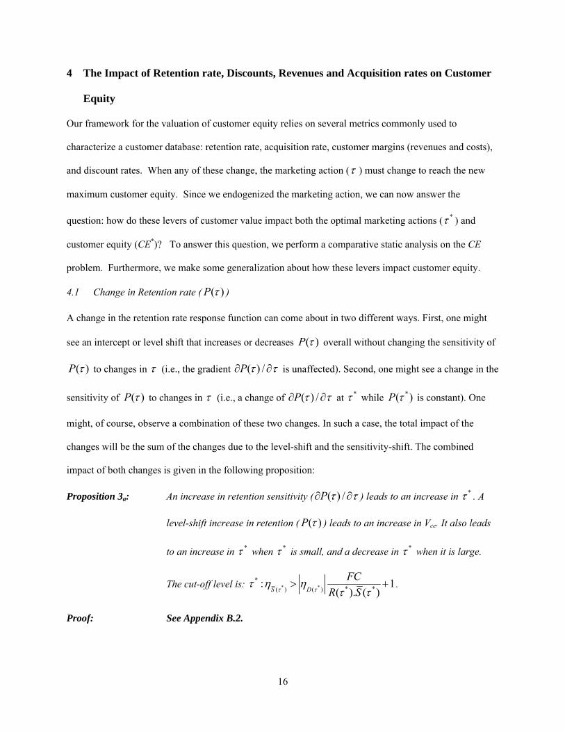
4.1 Change in Retention rate ( ( )P τ )

A change in the retention rate response function can come about in two different ways. First, one might

see an intercept or level shift that increases or decreases ( )P τ overall without changing the sensitivity of

( )P τ to changes in τ (i.e., the gradient ( ) /P τ τ∂ ∂ is unaffected). Second, one might see a change in the

sensitivity of ( )P τ to changes in τ (i.e., a change of ( ) /P τ τ∂ ∂ at *τ while *( )P τ is constant). One

might, of course, observe a combination of these two changes. In such a case, the total impact of the

changes will be the sum of the changes due to the level-shift and the sensitivity-shift. The combined

impact of both changes is given in the following proposition:

Proposition 3a: An increase in retention sensitivity ( ( ) /P τ τ∂ ∂ ) leads to an increase in *τ . A

level-shift increase in retention ( ( )P τ ) leads to an increase in Vce. It also leads

to an increase in *τ when *τ is small, and a decrease in *τ when it is large.

The cut-off level is: * **

* *( ) ( ): 1

( ). ( )S D

FCR Sτ τ

τ η ητ τ

> + .

Proof: See Appendix B.2.

16

The retention probability affects the FOC through both Sη and GM. Thus, when looking at changes in

( )P τ we need to consider the combined impact of both changes. In the case of a change in ( ) /P τ τ∂ ∂ ,

the situation is straightforward, as GM is unaffected and thus the increase in ( ) /P τ τ∂ ∂ leads to an

increase in the FOC through Sη . Hence, the firm would react by increasing its τ . In other words, an

increase in ( ) /P τ τ∂ ∂ means that the firm has more to gain by waiting a little longer between

communications, and since the system was at equilibrium before, it now leans in favor of a larger *τ .

In terms of database value, Vce is not directly affected by changes in ( ) /P τ τ∂ ∂ and thus, strictly

speaking, a change in ( ) /P τ τ∂ ∂ will not affect the database value. However, a change in ( ) /P τ τ∂ ∂

cannot reasonably arise without some change in ( )P τ . And thus, Vce will be affected through the change

in ( )P τ . It is straightforward to show that a level-shift increase in ( )P τ increases Vce. The envelope

theorem tells us that although *τ is affected by changes in P, when looking at the net impact on Vce, we

can ignore the (small) impact of changes in P on *τ , and simply look at the sign of . Here, we

have and thus V

/ceV∂ ∂P

0/ceV P∂ ∂ > ce is increasing in P.

In the case of a level-shift, the situation is made complex in that GM always increases when

( )P τ increases (which leads to a decrease in the FOC as Dη is negative), but the effect on Sη depends

on ( ) /P τ τ∂ ∂ . If we assume that ( )P τ is inverted-U shaped (increasing at a decreasing rate for small

τ — ( ) / 0P τ τ∂ ∂ > , , 2 2( ) / 0P τ τ∂ ∂ < τ pτ∀ < —then decreasing after some threshold—

( ) / 0P τ τ∂ ∂ < , pτ τ∀ > ) then we find that for small τ an intercept-shift increase in ( )P τ leads to an

increase in *τ , and for large τ it leads to a decrease in *τ . The difference in behavior comes from the

fact that when τ is small, an increase in ( )P τ has a large impact on the database size and spurs the

company to seek an even larger database while, when τ is large, an increase in retention allows the firm

to harvest the database to a greater extent.

17

4.2 Change in Expected Profit per Contact ( ( )R τ )

We study the impact of costs in the next section and focus here solely on ( )A τ . Similar to ( )P τ , ( )A τ

can be changed through an intercept-shift or through a change in sensitivity to τ . The situation is,

however, a bit more complex for ( )A τ than for ( )P τ because ( )P τ depends on ( )A τ . In other words,

defection depends in part on the content that is sent to customers. Thus, we must account not only for the

direct effect of a change in ( )A τ on the FOC, but also for indirect effects through changes in ( )P τ .

Proposition 3b: An increase in revenue per contact sensitivity ( ( ) /A τ τ∂ ∂ ) leads to an increase

in *τ . An intercept-shift in revenue per contact ( ( )A τ ) leads to an increase in

Vce. It also leads to a decrease in *τ when *τ is small to moderate, and an

increase in *τ when it is large. A lower-bound to the cut-off level

is: * 2: 1Sτ η τ= + .

Proof: See Appendix B.3.

The impact of ( )A τ on Vce follows from the envelope theorem. In terms of the impact of ( )A τ and

( ) /A τ τ∂ ∂ on *τ , the proof in Appendix B.3 is longer than for the previous proposition because of the

effects of A on P. The essence of the proposition is, however, straightforward. When the sensitivity of

revenue to longer τ increases, there is a pressure towards longer *τ . In case of a positive intercept-shift,

there is a tendency for the firm to take advantage of the shift by harvesting the database.

4.3 Change in Acquisition Rate (g)

Proposition 3c: An increase in acquisition rate leads to a decrease in *τ and an increase in Vce.

Proof: The proof is similar to the proof of Proposition 3a. Since S is a linear function of

g, the elasticity Sη does not depend on g. The only term in the FOC that depends on the acquisition rate

is the gross margin (through S ). Thus all we are interested in is the sign of:

18

2

( ). ( )( ). ( )

( ) .( ). ( )

GM R S FCg g R S

FC SR S g

τ ττ τ

ττ τ

∂ ∂ −=

∂ ∂

∂=

∂

Hence, 0GMg

∂>

∂ since

( ) 01 ( )

Sg Pτ τ

τ∂

=∂ −

> . Thus, given that GM acts as a multiplier to Dη , which is

negative, an increase in acquisition rate – through increased acquisition spending or increased acquisition

effectiveness – will lead to a decrease in *τ and conversely for a decrease in acquisition rate. Finally, the

increase in Vce follows from the envelope theorem and the fact that /ceV g∂ ∂ is positive.

This relationship between g and *τ is a direct result of treating customers as a resource. When

the resource is plentiful (g is high) the firm can harvest it; setting a low *τ . When the resource is scarce

(g is low), the firm must conserve it; setting a high *τ .

4.4 Change in Discount Rate (r)

Proposition 3d: An increase in discount rate leads to an increase in *τ and a decrease in Vce.

Proof: Although counterintuitive with regards to *τ , Proposition 3d is straightforward to

prove. To show that *τ increases in r, we first note that Rη , Sη , and GM are independent from r. Hence,

a change in discount rate will only affect Dη . This change is:

1 0, 0, 01 1 1

rD

r r r

r r e rr r e e e

τ

τ τ τ

η τ τ τ τ⎛ ⎞∂ ∂ −

= = − > ∀ >⎜ ⎟∂ ∂ − − −⎝ ⎠.>

The derivative of Dη with respect to r is positive for all positive r and τ .3 This implies that the optimal

reaction for a firm faced with an increase in discount rate is to increase its inter-communication interval.

This may seem counter-intuitive at first, as one might believe that increasing r makes future revenues less

attractive and, thus, one might want to decrease τ so as to realize more profits in the short-term.

19

What actually happens is that an increase in r leads to a decrease in the discount multiplier (D).

This decrease means that, holding everything else constant, the value of each name decreases, and thus

the value of the database decreases. This decrease must be offset by either an increase in database size

( S ) or an increase in expected profit per name per communication (R). Both can be accomplished by

increasing τ .

It is straightforward to show that as r increases, the value of the database decreases. Applying the

envelope theorem one more time we have:

( ) ( )( )2 0.

1 1

r rce

r r

V e eRS FC RS FCr r e e

τ τ

τ τ

τ∂ ∂ −= − = − <

∂ ∂ − −

Hence, an increase in r leads to both an increase in optimal inter-communication time ( *τ ) and a decrease

in database value (Vce). The impact of r on *τ could be used to study how a firm should vary its

communication time in response to interest rate variations. However, a more interesting study is how *τ

changes as a firm grows from a start-up to a large legitimate company. Indeed, a start-up is a risky

venture and its implicit discount rate will be high. As the firm grows, its future becomes less uncertain

and its discount rate diminishes. Proposition 3d states that in such case, the firm will decrease its inter-

communication time as it grows. This decrease in τ effectively shifts the firm from a “database growth”

regime to a “profit generation” regime as it now tries to extract more revenues from its database and

leaves itself less time between communication to replace the names lost.

4.5 Changes in Costs

The firm’s reaction to any increase in cost, whether fixed or variable, is to increase optimal inter-

communication interval. The intuition for this is straightforward. An increase in cost reduces per-

campaign profits. The firm must then increase *τ to try to boost its profits per campaign—reducing the

number of communications sent raises expected revenue per campaign.

Proposition 3e: An increase in fixed or variable costs leads to a decrease in Vce and an increase

in *τ .

20

Proof: Comes from 0ceVFC∂

<∂

, 0ceVVC∂

<∂

, 0R

VCη∂

>∂

, and 0GMVC

∂<

∂.

4.6 Take away

The study of the levers of customer value reveals some consistent patterns. The firm has two conflicting

objectives that it is trying to balance: database growth and database harvesting. Database growth involves

a long-term approach, so the marketer needs to adjust marketing actions so as to increase the database

size, ( S ). In the CE framework this can be achieved by reducing the communication frequency (i.e.

raising τ ). On the other hand, when the objective is to harvest the database, marketing actions need to be

adjusted so as to increase short-term revenues. This can be achieved by reducing the inter-

communication interval (i.e. decreasing τ —except in some occasions when τ is very small, in which

case both objectives are achieved by increasing τ ).

Whenever there is a change in the firm’s performance or in the environment that is beneficial to

the firm (e.g., higher return from acquisition, better retention rate, lower interest rate), the firm can adjust

its actions in a way that favors harvesting at the expense of growth (i.e., decrease τ ). Conversely, if the

change is detrimental (e.g., lower return per campaign, higher costs), the firm must counteract this change

by leaning more toward growth rather than harvesting (i.e., increase τ ).

5 Acquisition Policy

Now that we have discussed the key levers of the database value and can maximize the marketing actions

( *τ ) for any given acquisition policy, we can turn to the problem of optimizing acquisition. Indeed, we

have thus far assumed that acquisition expenditures were fixed. We were able to do this since Lemma 2

shows that the actual spending on name acquisition is separable from the optimization of τ , and therefore

only the acquisition rate matters for the derivation of the optimal inter-communication interval. The

implication of this result is that the marketer first needs to derive the optimal τ for a given acquisition

rate (Section Error! Reference source not found.), and then optimize acquisition spending given the

21

solution for *τ . Section 4 ignored acquisition except for the finding that an increase in acquisition rate

leads to a decrease in *τ (Proposition 3c).

Our goal for this section is to derive the optimal acquisition policy (g*) as a function of the

optimal marketing policy *τ . We found that a higher customer acquisition rate leads to greater database

size, and larger revenues, but these benefits must be offset against the cost of acquiring these customers.

It is critical, for this analysis, to understand that the acquisition costs correspond to a stream of customers

over time, rather than a one-time payment for such customers.

Formally, since, by Proposition 2, we can separate the optimization of the optimal inter-

communication interval ( *τ ) from the optimal acquisition rate, then *τ can be expressed as a function of

acquisition spending. Thus we can find the optimal expenditure on acquisition by taking the derivative of

CE with respect to g. The optimum is found when marginal revenues are equal to marginal costs. We

formalize this in the following proposition:

Proposition 4: If the periodicity at which the acquisition expenditures are recognized is equal to

the periodicity of the communications (i.e., * 1τ = ), then optimal acquisition rate

occurs when the marginal acquisition cost per name is equal to the non-

discounted expected revenues from the name.

Proof: The firm will increase its acquisition spending until the marginal profit generated

by the last acquired name is equal to the marginal costs of acquiring names. This point can be found by

studying the first-order condition for acquisition cost:

*

*

**

*

0 0

( ) 01 ( ) 11

r r

rr

MR MC

CE e e AQRg P e ge

τ

τ

τττ> >

∂ ∂= −∂ − − ∂−

= . (13)

Rearranging (13) to isolate the maximum amount one should be willing to pay to acquire one more

customer, we obtain:

22

*

*

* *

*

1 . ( )1 (1

r r

r r

I II

AQ e e Rg e Pe

τ

τ )τ τ

τ−∂ =

∂ −−. (14)

There are two components, labeled I and II, to this equation. The first term is a discount adjustment factor

that corrects the expected profits for any discrepancies between the interval at which expenses are

recognized and profits are realized. If expenses and profits are recognized at different time intervals, say

monthly expenses and quarterly newsletters, the firm needs to adjust its acquisition expenditure to reflect

the fact that profits will lag or precede expenditures.4 However, when acquisition expenses are recognized

at the same interval as the revenue (i.e., * 1τ = ) this term is equal to 1. In this case, we can simplify (14)

to show that marginal cost must equal expected marginal revenues:

*

*

( )1 (

AQ Rg P

τ)τ

∂ =∂ −

. (15)

The importance of Proposition 4 is that the revenues are not discounted. In traditional CLV

calculation (see equation (11)) one discounts future revenues, thus the marginal acquisition costs should

not be greater than the CLV or:

*

**

**

( )( )( )( ) 1

r

r

r

AQ e RRPg e Pe

τ

τ

τ

ττττ

∂= =

∂ − −. (16)

In other words, the optimal spending based on the Customer Equity perspective (15) is greater than that

based on from a CLV perspective (16). This parallels Proposition 1 such that the CLV framework not only

leads to sub-optimal *τ ’s, but also sub-optimal acquisition expenditures ( *( )AQ τ ).

To understand why future revenues should not be discounted when setting the optimal policy,

consider figures 1a and 1b. Figure 1a represents the evolution of one cohort. Figure 1b represents the

make up of the database as new cohorts are acquired and old ones shrink. Focusing on the tenth year

(Y10), one can see that at any point in time, the database contains the names acquired as part of the latest

cohort, plus the names from the previous cohort that survived one period, plus the names of the cohort

23

before that survived two periods, and so on. Hence, by collating individuals across cohorts we can

recreate the profile of a single cohort. Thus, the revenues generated by the database in each period are

equal to the revenues generated by one cohort over its entire lifetime. Profitability at stationarity requires

that the acquisition costs in any period are more than offset by the profits generated during that period.

Hence, profitability only requires that the costs of acquiring a cohort are less than the (undiscounted)

revenues generated by one cohort. There is no discounting of future revenues, because at steady state,

acquisition costs are offset by current rather than future revenues. It is an inter-cohort revenue matching

rather than an inter-temporal one.

A side benefit of working with non-discounted revenues is that it allows us to relax the

assumptions of constant retention rate and revenues. Indeed, looking at Figure 2a we see a cohort profile

where retention is not constant over the life of its members. Retention is low in the first year, high for the

next four years, then steady for the remaining years. This uneven retention violates our assumption of

constant retention rate which is necessary to simplify the infinite sum of future revenues into the simple

equation that is (9). However, as is demonstrated by figure 2b, the database size in this case is still equal

to the sum of the cohort size over its life, and the revenues generated by the database in one period are

still equal to the revenues generated by a cohort over its life. Thus, Lemma 1 will still hold in that there is

a fixed long-term size to the database (the actual size will not be .

1 (g

P )τ

τ− as P is not constant over time,

but it can still be calculated, we show an example of this in section 6.1). Further, one can still use the first

order condition developed in (12) to maximize the database value. Finally, equation (15) still applies, and

we can compute the maximum acquisition spending to one period of database revenues divided by the

number of new customers needed to maintain steady state size.

6 Heterogeneity

An important assumption was made about customers being identical in terms of key constituents of the

CLV, the revenue function, the retention function and acquisition policy. We thereby assumed that the

database value could be expressed as a function of an “average” consumer. This simplified view the

24

derivation of many of the results, but we need to understand how robust the results are if we relax this

assumption.

First note that marketers deal with two types of heterogeneity: observed and unobserved. This

leads to two questions. First, what happens when customers are treated as identical when they are not

(unobserved heterogeneity)? Second, how does our framework change, and is it still applicable, when

heterogeneity is observed and the marketer treats different customers differently by sending different

communications to different groups of customers, or send communications at different rates to different

customers?

6.1 Unobserved heterogeneity

Customers can be heterogeneous in their retention probability (P) and/or their expected return from each

communication (R). If consumers have identical retention probabilities, but are heterogeneous in their

expected return, then, if all customers are treated as being identical, the average expected return ( R ) can

be used to maximize profits. Indeed, let f(R) be the probability density function of R. The expected

database value is obtained by integrating out customer equity across customers:

( ) ( )[ ] ( )1 1

r r

ce r r

e eE V RS FC f R dR RS FCe e

τ τ

τ τ= − = −− −∫ .

Taking the same approach is a little more complicated for heterogeneity in the retention rate.

Indeed, P appears on the denominator of CE through S . Thus, going back to Little’s Law, we need to

compute:

1 .. . [ ] .1 1 [

gS g EP E P]

ττ= ≠− −

The difference stems from the fact that customers with higher retention rates stay in the database longer

than customers with lower retention rates. For instance, if we assume that the acquisition efforts yield a

stream of customers whose retention rate has a Beta distribution, ( , )α βΒ with 1β > 5, then we have:

1 1 1 2

0 0

( ) ( ) (1 ) .1 ( ) ( )f PS g dP g P P dP

Pα βα βτ τ

α β− −Γ +

= = −− Γ Γ∫ ∫

25

Since , we have: ( 1) (n nΓ + = Γ )n

1 1 2

0

1

( 1) ( 1) .(1 ) ,( 1) ( ) ( 1) 1

( 1

gS g P P dPα β

)

α β α β ττ αβ α βα β

− −

=

+ − Γ + −= −

− Γ Γ − −+ −

∫ =

where we recognize the term ( 1)

αα β+ −

as the expected value of a ( , 1)α βΒ − . Hence, if the

heterogeneity in retention rate in the acquisition stream is characterized by a ( , )α βΒ , then the marketer

should optimize its database using the expected value of a ( , 1)α βΒ − as its average P.

6.2 Observed Heterogeneity

A firm faced with observed heterogeneity can adapt its marketing actions in two ways. The traditional

method used by marketers is to segment customers into mutually exclusive segments based on their

purchase behavior and then treat each customer segment as homogenous. Airlines, with their tiered

frequent flyer programs, are classic examples of this approach. Proponents of Customer Relationship

Management (CRM) propose a more radical approach where each customer is able to receive an

individually tailored marketing communication.

It is easy to see that the CE approach is appropriate for the traditional customer segmentation

approach. One can optimize each segment’s marketing communications and overall value separately, as a

function of each segment’s acquisition, margins, and retention rates. One can also easily compute the

benefits of having more or less segments by comparing the segment values in an N segment world to

those in an N+1 segment world. The trade-off one makes when increasing the number of segments is that

revenues should increase with the number of segments as one can better customize the marketing

communications when the segments become more homogenous; but, communication costs will also

increase as different communication must be created for different segments. This naturally leads to an

optimal number of segments.

The promises of CRM are to make the customization costs so low that it now becomes feasible to

have segments of size one. If this promise were realized, one could argue that a CLV model is more

26

appropriate than a CE model. Indeed, if segments are of size one then they truly are depletable. When

the segment member defects; the segment is depleted. Newly acquired customers constitute their own

segments rather than replenishing pre-existing segments. If all decision variables (acquisition spending,

communication frequency, communication content, etc.) are optimized at the individual level independent

of other individuals, then the CLV approach is the correct one. However, that is not what CRM actually

entails.

What CRM proposes to do in practice is to develop a set of rules or models that, when applied to

the information known about the firm’s customer, yield a customized marketing message (Winer 2001).

The nature and the amount of customization varies across applications. For instance, American Airlines

uses CRM to select which WebFares to advertise to each of its frequent flyers in its weekly emails.

Citibank uses CRM to direct callers to its toll free lines to the sales person that is most adept at selling the

type of products that their predictive model selected as a likely candidate for cross-selling. Amazon.com

uses CRM to try to up-sell its customers by offering them bundles of books they might be interested in. In

each of these examples, different customers will experience different offerings. Different frequent flyers

will be alerted of different promotional fares depending on the cities they fly most; different readers will

be offered different book bundles depending on the books they are searching for. Nevertheless, the set of

rules or models that are used to generate these offers will be identical for all frequent flyers, or all

Amazon customers. The output will be different, but the process will be identical. Further, the costs of

creating the rules and communication templates will be shared across all individuals rather than borne

individually. As such, the CE framework developed here still applies. The CRM objectives will be to

develop the set of rules that maximize overall CE rather than any specific individual’s CLV. When doing

so, it is critical to use the appropriate objective function. This will be achieved by considering the impact

of the CRM efforts on retention and amounts spent and maximize the long term database value just as has

been done in this paper with the inter-communication interval (τ ).

27

6.3 Simulation

To illustrate the CE approach for database optimization, and to demonstrate that the CE framework is

robust to a stochastic environment, we conducted a simulation where the acquisition, retention, and

purchase processes were stochastic yielding a wide heterogeneity in customers. We simulate a process by

which a company acquires customers on a continuous basis. Once per period, the firm sends a

communication to the customers who are still active. These customers respond to the offers in a stochastic

manner and have an individual level retention rate. In line with the queuing theory literature, we assume

an exponential arrival rate for customers and model the per-period acquisition process using a Poisson

process (Cooper 1981). For each acquired customer, we draw a retention probability from a Beta(3,3)

distribution. In each period, each active customer generates a purchase whose monetary value is drawn

from a Uniform(0,50) distribution using a different draw from the distribution for each customer in each

period. Further, to illustrate what happens when the acquisition policy changes, we run the simulation for

250 periods with the acquisition stream set as a Poisson(7,500) (i.e., the mean number of customers

acquired per period is 7,500), then we increase the arrival rate to produce an average of 10,000 names per

period.

Our theory predicts that if the retention probabilities in the incoming customer name stream are

distributed Beta(3,3), then, in the long run, the retention probabilities of the members of the database will

be distributed Beta(3,2). To check this, we plot (Figure 4a) the distribution of the retention probabilities

of all the names acquired in our simulation (in grey) alongside the distribution of the retention

probabilities of the names in the database at the end of the 500-period simulation (in black). As one can

see, the simulation results match our expectation.

A Beta(3,2) has a mean of 3/5. Thus, Lemma 1 predicts that the size of the database will be

7,500/(3/5)=18,750 during the first 250 periods of the simulation. It will then increase to 25,000 during

the next 250 periods. Further, given that the purchases are distributed Uniform(0,50), the expected

revenue during the first 250 periods will be $468,750; increasing to $625,000 in the next 250 periods. We

show the period-by-period database size and revenues in Figures 4b and 4c respectively. Again, our

28

model outcomes are confirmed. Once the database reaches its steady-state size it does not deviate much

from the expected values. Given our process, it seems to take about 20 periods for the database to grow

from 0 names to the steady-state. When the acquisition rate increases to 10,000 names per period, it takes

about 15 periods for the database to adjust its size. Finally, note that once the steady state has been

reached, the database generates $625,000 every period as long as the acquisition process generates 10,000

names. Therefore, as long as acquisition spending is less than $62.50 per acquired customers, the firm

will generate profits every period. This upper bound of $62.50 is equal to the undiscounted expected cash

flow ($25 per period for 2.5 periods) as predicted by our model rather than the discounted cash flow

predicted by the CLV approach.

7 Managerial Implications and Conclusion

The lifetime value of a firm’s customer base depends both on the acquisition process used by the firm and

the marketing actions targeted at these customers. To take both aspects into account, we draw on the

theory of optimal resource management to revisit the concept of customer lifetime value. Our contention

is that customers are a renewable resource and hence marketing actions directed at acquiring and

extracting revenues from customers should take a long-term value-maximization approach. Thus we

study the implications of moving from Customer Lifetime Value maximization to Customer Equity

maximization. To answer the first questions raised in the introduction is (Does CLV maximization equate

to CE maximization?), our findings indicate that disregarding future acquisition leads to sub-optimal

acquisition (Proposition 4) and revenue extraction strategies (Proposition 1).

Following on from this, our second research question addresses what is the proper benchmark to

use to guide customer acquisition policy. Of significance is our finding that the firm is able to spend

more on acquiring a new customer if it were to use the CE approach, than if it were to estimate the value

of a customer using the CLV approach.

To answer the final research questions raised (What is the appropriate metric, how is it computed

and maximized?), we first need to consider how the database value is impacted by actions of the

marketer. As we summarized in Proposition 2, our model of customer equity directly accounts for the

29

impact of marketing actions on the value of a firm’s customer assets. This allows us to derive the optimal

actions for the firm, and we derive the long-term steady-state size of a firm’s customer base (Lemma 1).

Our first-order condition for the maximization of customer equity (Proposition 2) shows that a firm

should adapt its marketing actions to changes in the critical factors that impact database value. The

strength of the first-order condition derived in Proposition 2 is that it is easy to optimize empirically. The

firm can run a series of tests to estimate the various elasticities and infer from them if it should increase or

decrease its communication periodicity. This is simplified by the fact that customer equity has a unique

maximum. The first-order condition also lends itself well to static comparisons (Propositions 3a to 3d).

This exercise shows how firms are attempting to balance two conflicting objectives: database growth and

database harvesting. Whenever there is a change in the firm’s performance or in the environment that is

beneficial to the firm (e.g., higher return from acquisition, better retention rate, lower interest rate), the

firm should adjust its actions in a way that favors harvesting at the expense of growth. Conversely, if the

change is detrimental (e.g., lower return per campaign, higher costs), the firm must counteract this change

by leaning more toward growth rather than harvesting.

We finish the paper with a discussion of customer heterogeneity. We show that our model is

robust to unobserved heterogeneity. The learning point there is that ignoring heterogeneity in customers’

valuation of the communication is less of an issue than ignoring customer heterogeneity in retention rate.

We recognize several limitations inherent in this study. We made specific assumptions regarding

the relationship between customer retention and the firm’s communication strategy, both in terms of

timing (through τ ) and in content (through the relationship between A and P) that could be relaxed in

future work. We have also dissociated the issue of heterogeneity from our main findings. Finally, we have

only concerned ourselves with the steady state regime without studying the path to this steady state.

More can certainly be done on those fronts. Further work also needs to be done to incorporate the impact

of competitive actions and reactions on the measurement of customer equity. This might potentially be

done by folding our approach with a theoretical model such as the one developed by Fruchter and Zhang

30

(2004). We believe, however, that the framework presented in this study is a useful starting point for such

a competitive analysis.

References

Bayon, Thomas, Jens Gutsche, and Hans Bauer (2002), “Customer Equity Marketing: Touching the

Intangible,” European Management Journal, 20 (3), 213-22.

Berger, Paul D., Ruth N. Bolton, Douglas Bowman, Elten Briggs, V. Kumar, A. Parasuraman, and Creed

Terry (2002), “Marketing Actions and the Value of Customer Assets: A Framework for Customer

Asset Management,” Journal of Service Research, 5 (1), 39-54.

Berger, Paul D. and Nada I. Nasr (1998), “Customer Life Time Value: Marketing Models and

Applications,” Journal of Interactive Marketing, 12 (1), 17-30.

Blattberg, Robert C. and John Deighton (1996), “Manage Marketing by the Customer Equity Test,”

Harvard Business Review, July-August, 136-144.

Cooper, Robert B. (1981), Introduction to queuing theory, Elsevier North Holland, New York.

Fruchter, Gila E. and John Z. Zhang (2004), “Dynamic Targeted Promotions: A Customer Retention and

Acquisition Perspective,” Journal of Service Research, 7 (1), 3-19.

Gupta, Sunil and Donald R. Lehmann (2003), “Customers As Assets,” Journal of Interactive Marketing,

17(1), 9-24.

Gupta, Sunil, Donald R. Lehmann, and Jennifer Ames Stuart (2004), “Valuing Customers,” Journal of

Marketing Research, XLI (February), 7-18.

Hwang, Hyunseok, Taesoo Jung, and Euiho Suh (2004), “An LTV model and customer segmentation

based on customer value: a cose study on the wireless telecommunication industry,” Expert

Systems with Applications, 26(2004), 181-8.

31

Libai, Barak, Das Narayandas, and Clive Humby (2002), “Toward an Individual Customer Profitability

Model: A Segment-Based Approach,” Journal of Service Research, 5 (1), 69-76.

Little, John D.C. (1961), “A Proof of the Queuing Formula: L Wλ= ,” Operations Research, 9 (May),

383-387.

Rust, Roland T., Katherine N. Lemon, and Valarie A. Zeithaml (2004), “Return on Marketing: Using

Customer Equity to Focus Marketing Strategy,” Journal of Marketing, 68 (January), 109-27.

Sweeny, James L. (1992), “Economic Theory of Depletable Resources: An Introduction,” in Handbook of

Natural Resources and Energy Economics, Vol. 3, ed. by A. V. Kneese and J. L. Sweeney, North-

Holland.

Wang, Paul and Ted Spiegel (1994) “Database Marketing and its Measurement of Success: Designing a

Managerial Instrument to Calculate the Value of a Repeat Customer Database,” Journal of Direct

Marketing, 8(2), Spring, 73-81.

Winer, Russell S. (2001), “A Framework for Customer Relationship Management,” California

Management Review, 43 (Summer), 89-105.

Zeithaml, Valarie A., Roland T. Rust, and Katherine N. Lemon (2001), “The Customer Pyramid: Creating

and Serving Profitable Customers,” California Management Review, 43 (4), 118-42.

32

Appendix A: Proof of Lemma 1 and Proposition 1

A.1 Proof of Lemma 1. Let ( )P τ be the proportion of the database that is retained from one campaign to the next, given that τ

is the fixed inter-campaign time interval. Let the acquisition stream be ( ) .g gτ τ= . If the firm begins

with a database size at 0S S≠ , we show that the long-term stationary value of the database is still S . To find this value, solve the Law of Motion for the size of the database as:

.. ( ) . .

1 ( )gS S P g

Pττ τ

τ= + =

−

What if the database size is not at the stationary value? Then, ifτ is constant, the state variable converges to the stationary value. To see this, pick any arbitrary value for the starting size of the database e.g. pick any 0ε ≠ such that iS S< or iS S> e.g.:

. .

1 ( )igS

Pτ ε

τ= +

−

so that for the next period:

1. .( ) . ( ) . . )

1 ( ) 1 ( )i ig gS S P g P g P

P Pτ ττ τ ε τ τ

τ τ+

⎛ ⎞= + = + + = +⎜ ⎟− −⎝ ⎠

ε τ(

and for any n>0,

. ( )

1 ( , )n

i ngS P

P kτ ε ττ+ = +

−

and lim i nnS +→∞

= S , since ( ) (0,1)P τ ∈ and therefore . ( ) 0 as nP nε τ → →∞

A.2 Maximization of Customer Value versus Customer Equity. Assume that we look at the equilibrium conditions so that iS S= . The value of an individual customer name is defined as:

0

( ) ( ) ( ) .( )

rir i

clv ri

FC FC eV e P R RS S e

ττ

ττ τ τP τ

∞−

=

⎛ ⎞ ⎛ ⎞= − = −⎜ ⎟ ⎜ ⎟ −⎝ ⎠ ⎝ ⎠∑

The database value, is defined as:

( ) ( )0

( ) ( ) .1

rir

ce ri

eV e R S FC R S FCe

ττ

ττ τ∞

−

=

= − = −−∑

Hence, we have the database value as a function of the customer value: ( ) .1

r

ce clv r

e PV V Se

τ

τ

τ−=

−

To maximize, we differentiate with respect to τ : ( ) ( ) .1 1

r rce clv

clvr r

V Ve P e PS V Se e

τ τ

τ τ

τ ττ τ τ

∂ ∂− ∂= +

∂ − ∂ ∂−−

Hence, maximizing the CLV and the CE will be identical iff:

33

00? 00 0

( ) ( ) 01 1

r rce clv

clvr r

V Ve P e PS V Se e

τ τ

τ τ

τ ττ τ τ

≠=≠ =

∂ ∂− ∂ −= +

∂ − ∂ ∂ −?

= .

The fourth term ( )1

r

r

e PSe

τ

τ

ττ

⎛ ⎞∂ −⎜ ∂ −⎝ ⎠

⎟ will be equal to 0 iff: ( )1

0r

r

S e Pe

τ

ττ

η η−−

+ = , or ( )1

.r

r

S e Pe

τ

ττ

η η−−

= −

We know that ( )1

1 ( )SP

Pτ τητ τ

∂= +

∂ −, we now need to compute ( )

1

r

re P

e

τ

ττ

η−−

:

( )( )

( )

( ) ( )( )21 1 1

( )1 ( ) .1 1

Pr r rre e P rere Pr re e re

r re P rePrrer re e

ττ τ τττ τ ττ ττ τ

τ τττττ ττ

∂− −∂ − ∂= −∂ − − −

⎛ ⎞−⎜ ⎟∂= − −⎜ ⎟∂− −⎜ ⎟

⎝ ⎠

Thus:

( )

( )( )

( )1

( )1 ( )( )1 11

1 ( ) ( ) .( )1 ( )

r

r

re Pe

r

rr r

r re P rePrrer r e Pe ee

P Prree Pe e P

τ

τ

ττ

τ

ττ τ

τ τττ ττη τ τ ττ

τ τ ττττ ττ

−−

⎛ ⎞−⎜ ⎟∂= − −⎜ ⎟ −∂− −⎜ ⎟

⎝ ⎠ −⎡ ⎤⎛ ⎞− ∂⎢ ⎥⎜ ⎟= − +

⎜ ⎟ ∂ −− −⎢ ⎥⎝ ⎠⎣ ⎦

This means that Sη and ( )1

r

re P

e

τ

ττ

η−−

− are both affine transformations of ( )P ττ

∂∂

, and thus will be equal for

all ( )P ττ

∂∂

iff both their intercepts and their slopes are equal, or:

( )( )1 ( )11 (

.1 ( ) ( )

r r

r

Prree e P

P e P

τ τ

τ

ττττ

τ ττ τ

⎛ ⎞−⎜ ⎟=⎜ ⎟− −⎝ ⎠

=− −

) and

The second condition gives us that they will be equal only when 0τ = . Applying l’Hospital Rule to the first condition we find that, at the limit for 0τ → , the first condition is also satisfied. Hence, this shows

that it will only be for 0τ = that ( )1

r

r

e pSe

τ

τ

ττ∂ −∂ −

. And thus, maximizing the Vclv and the Vce lead to the

same optimal only when , which cannot happen since at * 0τ = 0τ = the database value is negative ( ). QED (0)ceV = −∞

34

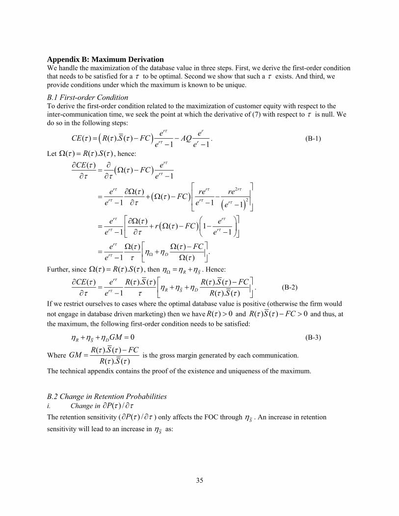
Appendix B: Maximum Derivation We handle the maximization of the database value in three steps. First, we derive the first-order condition that needs to be satisfied for a τ to be optimal. Second we show that such a τ exists. And third, we provide conditions under which the maximum is known to be unique.

B.1 First-order Condition To derive the first-order condition related to the maximization of customer equity with respect to the inter-communication time, we seek the point at which the derivative of (7) with respect to τ is null. We do so in the following steps:

( )( ) ( ). ( )1 1

r r

r

e eCE R S FC AQe e

τ

ττ τ τ= − − r− −. (B-1)

Let ( ) ( ). ( )R Sτ τ τΩ = , hence:

( )

( )( )

( )

2

2

( ) ( )1

( ) ( )1 1 1

( ) ( ) 11 1

( ) ( ) .1 ( )

r

r

r r

r r r

r r

r r

r

Dr

CE eFCe

e reFCe e e

e er FCe e

e FCe

τ

τ

τ τ

τ τ τ

τ τ

τ τ

τ

τ

τ ττ τ

τ ττ

τ ττ

τ τη ητ τΩ

∂ ∂= Ω −

∂ ∂ −rre τ⎡ ⎤∂Ω ⎢ ⎥= + Ω − −

⎢ ⎥− ∂ − −⎣ ⎦⎡ ⎤⎛ ⎞∂Ω

= + Ω − −⎢ ⎥⎜ ⎟− ∂ −⎝ ⎠⎣ ⎦⎡ ⎤Ω Ω −

= +⎢ ⎥− Ω⎣ ⎦

Further, since ( ) ( ). ( )R Sτ τ τΩ = , then R Sη η ηΩ = + . Hence:

( ) ( ). ( ) ( ). ( )1 (

r

R DSr

CE e R S R S FCe R

τ

τ

τ τ τ τ τη η ητ τ τ

⎡ ⎤∂ −= + +⎢ ⎥∂ − ⎣ ⎦). ( )S τ

. (B-2)

If we restrict ourselves to cases where the optimal database value is positive (otherwise the firm would not engage in database driven marketing) then we have ( ) 0R τ > and ( ) ( ) 0R S FCτ τ − > and thus, at the maximum, the following first-order condition needs to be satisfied:

0R DS GMη η η+ + = (B-3)

Where ( ). ( )

( ). ( )R S FCGM

R Sτ τ

τ τ−

= is the gross margin generated by each communication.

The technical appendix contains the proof of the existence and uniqueness of the maximum.

B.2 Change in Retention Probabilities i. Change in ( ) /P τ τ∂ ∂ The retention sensitivity ( ( ) /P τ τ∂ ∂ ) only affects the FOC through Sη . An increase in retention

sensitivity will lead to an increase in Sη as:

35

( )1( ) ( ) ( ) 1 ( )( ) ( )

0.1 ( )

S PP P P

P

η τ ττ τ τ ττ τ

ττ

∂ ⎡ ⎤∂ ∂= +⎢ ⎥∂ ∂ ∂ −⎣ ⎦

∂ ∂

= >−

This increase in Sη will lead the firm to increase its τ to reach maximum profits. ii. Intercept-shift in ( )P τ We look here at the change in FOC resulting from an intercept-shift increase in retention probabilities. That is:

1 0

1

( ) ( )( ) ( ) .

P PP P

pτ ττ ττ τ

= +∂ ∂

=∂ ∂

Since ( )R τ and D are both independent from ( )P τ , we have 0 0

0 and 0R

p pDη η∂ ∂

= =∂ ∂

. Further:

( )

1

0 0 1

0 0

20

( )11 ( )

( ) 11 ( )

( ) .1 ( )

S Pp p P

Pp P p

PP p

η τ ττ τ

τ ττ τ

τ τττ

∂ ⎡ ∂∂= +⎢ ⎥∂ ∂ ∂ −⎣ ⎦

⎡ ⎤∂ ∂= ⎢ ⎥∂ ∂ − −⎣ ⎦

∂=

∂− −

⎤

(B-4)

Hence, 0/S pη∂ ∂ has the same sign as ( ) /P τ τ∂ ∂ . For small τ , where ( ) /P τ τ∂ ∂ is positive, the

intercept-shift will have a positive impact on Sη . For large τ , where ( ) /P τ τ∂ ∂ is negative, the impact will be negative. For GM we have:

0 0

0

20

0

( ). ( )( ). ( )

( ). ( )( ) .

( ) ( )

GM R S FCp p R S

FCp R SFC S

R S p

τ ττ τ

τ τ

ττ τ

>

∂ ∂ −=

∂ ∂∂

= −∂

∂=

∂

(B-5)

And:

( )

0 0 0

20

( ) .1 ( )

. 0.1 ( )

S gp p P p

gP p

τ ττ

ττ

∂ ∂=

∂ ∂ − −

=− −

> (B-6)

36

Hence, an intercept-shift increase in ( )P τ leads to an increase in GM that leads to a decrease in FOC. Putting (B-4), (B-5), and (B-6) back into the FOC, we have that an intercept-shift increase in ( )P τ will

lead to higher *τ if:

( ) ( )2 2 2

( ) .( ) ( )1 ( ) 1 ( )

( )( ) ( ). ( )

( )1 ( ). ( )

1.( ). ( )

Do o

D

D

DS

P gR SP p P p

P g FCS R S

P FCP R S

FCR S

FCτ τ τητ τ ττ τ

τ ητ τ τ ττ τ ητ τ τ

η ητ τ

∂>

∂− − − −

∂ >∂

∂ >∂ −

> + (B-7)

That is, if we assume that ( )P τ is inverted-U shape, *τ increases for small *τ when there is an

intercept-shift in ( )P τ , and decreases for large *τ .

B.3 Change in Revenue per Contact i. Change in ( ) /A τ τ∂ ∂ The revenue sensitivity affects the FOC through both Rη and Sη . We have:

( )( ) ( ) ( )

0.( )

R AA A A V

A VC

Cη τ ττ τ τ ττ τ

ττ

∂ ∂ ∂=

∂ ∂ ∂ −∂ ∂∂ ∂

= >−

and

2

( )1( ) ( ) 1 ( )

( )1( ) 1 ( )

( ) ( )1( ) 1 ( )

( )( ) ( )1( ) 1 ( )

1

S PA A P

A cfA P

f x A cA P x

Af x A

A P x

η τ ττ τ τ ττ τ

τ ττ τ τ ττ

τ ττ τ τ ττ

ττ ττ

τ τ τ ττ

∂ ⎡ ⎤∂ ∂= +⎢ ⎥∂ ∂ ∂ −⎣ ⎦∂ ∂

∂ ∂⎡ ⎤∂ ∂ −⎛ ⎞= + ⎜ ⎟⎢ ⎥∂ − ∂ ⎝ ⎠⎣ ⎦∂

∂⎡ ⎤∂ ∂ ∂ −⎡ ⎤= +⎢ ⎥⎢ ⎥∂ − ∂ ∂ ⎣ ⎦⎣ ⎦∂

∂⎡ ∂⎛ ⎞⎢ ⎥⎜ ⎟∂ ∂ ∂= + −⎢ ⎥⎜ ⎟∂ − ∂⎢ ⎥⎜ ⎟∂⎢ ⎥∂ ⎝ ⎠⎣ ⎦

=

c⎤

−

( ) 0.1 ( )

f xP xτ

∂>

− ∂

37

Hence, the database sensitivity to τ increases when the sensitivity of the revenue increases, creating a compounding effect that leads the firm to increase its optimal sending rate ( *τ ).

iii. Intercept-shift in ( )A τ An intercept-shift in ( )A τ will be felt through Rη , Sη , and GM. Thus, we compute the following:

1 0

1

( ) ( )( ) ( )

A A aA Aτ ττ ττ τ

= +∂ ∂

=∂ ∂

( )

0 0

2

( )( )

( )( )

0( )

R

R

Aa a A V

AA VC

R

η τ ττ τ

τ ττ τητ

∂ ∂ ∂=

∂ ∂ ∂ −∂ −

=∂ −

−= <

C

0 0

( ) ( )

1 ( ) 0

P Afa a

f xx

τ ττ

τ

∂ ∂ −⎛ ⎞= ⎜ ⎟∂ ∂ ⎝ ⎠∂

= >∂

c

20 0

2

( )( ) ( ) 1 ( )

1 ( ) 0

Pf x A A c

a a xf x

x

ττ τττ τ τ

τ

∂∂ ∂ ⎡∂ ∂ − ⎤⎛ ⎞∂ = −⎜ ⎟⎢ ⎥∂ ∂ ∂ ∂⎝ ⎠⎣ ⎦∂

= − <∂

( )

0 0

02

0

.1 ( )

( )

.1 ( )

( )1 ( )

1 ( ) 01 ( )

S ga a P

Pag

P

S PP a

S f xP x

τττ

ττ

ττ

τ τ

⎡ ⎤∂ ∂= ⎢ ⎥∂ ∂ −⎣ ⎦

∂∂

=−

∂=

− ∂

∂= >

− ∂

38

( )

( )

0 0

0 02

2

( ). ( )

( ) ( ). ( ) ( ).

( ). ( )

( ). ( ) 1 ( )( )1 ( )( ). ( )

1 1 1 ( ) 0( ). ( ) ( ) 1 ( )

GM FCa a R S

R SS Ra aFC

R S

R S f xSP xFC

R S

FC f xR S R P x

τ τ

τ ττ τ

τ τ

τ τττ τ

τ τ

τ τ τ τ τ

∂ ∂= −

∂ ∂

⎛ ⎞∂ ∂+⎜ ⎟∂ ∂⎜ ⎟=⎜ ⎟⎜ ⎟⎝ ⎠⎛ ⎞∂

+⎜ ⎟− ∂⎜ ⎟=⎜ ⎟⎜ ⎟⎝ ⎠

⎛ ⎞∂= +⎜ ⎟− ∂⎝ ⎠

>

( )

( )

( )

0 0

02

0

( )11 ( )

( )( )( )

1 ( ) 1 ( )1 ( )21 ( ) ( )

2 21 ( ) 1 ( )

1 ( ) (1 ( )2(1 ( ))

S Pa a P

PPaP

P a P

) .

f xxf x P

P x P

f x PPxP

η τ ττ τ

τττ ττ ττ τ τ

τ τ τττ ττ τ

ττττ τ

∂ ⎡ ⎤∂ ∂= +⎢ ⎥∂ ∂ ∂ −⎣ ⎦

∂∂∂ ∂∂∂= +

− ∂ ∂ −

− ∂∂− ∂ ∂

= +− ∂ ∂ −

− ∂ ∂⎡ ⎤= −⎢ ⎥∂ ∂⎣ ⎦−+

Hence, 0/S aη∂ ∂ is negative for small to moderate levels of *τ (i.e., * * *:1 ( ) ( ) /P Pτ τ τ τ− > −∂ ∂ ) and

positive for larger *τ . Thus, for small to moderate *τ , the negative impacts on Rη , Sη and the positive

impact on GM will both yield a smaller *τ . For large *τ , the net impact might be positive. The point at which the effect reverses itself is given by:

( )( )2

1 ( ) ( ) 1 1 1 ( ): 1 ( )( ) ( ). ( ) ( ) 1 ( )1 ( )

RD

P f x FC fPR x R S RPη ττ τ τ ητ τ τ τ τ τ ττ τ

⎛ ⎞− − ∂ ∂ ∂⎛ ⎞+ − − + +⎜ ⎟⎜ ⎟∂ ∂ −⎝ ⎠− ⎝ ⎠0x

P x=

∂

. This expression is not tractable, but a lower-bound on *τ is given by:

( )* ( ): 1P P( )ττ τ ττ

∂= −

∂

or . * 2: 1Sτ η τ= +

39

(1 )d+ re1 NPV calculations traditionally uses 1/ as the discount factor. To make our derivations simpler, we use −

instead. The two formulations are equivalent if we set r dln(1 )= +

0

. 2 There is conflicting evidence regarding whether revenues per customer increase or decrease as a function of the

length of the relationship with the firm. Gupta et al (2004) fail to find any systematic pattern in per customer

revenues for the companies they studied.

= , r e , and for all 1 0r reτ ττ = − = 03 To see this, note that at τ τ > ,

2 1r r r r rr e re r e e reτ τ τ τ ττ ττ τ∂ ∂

= + > − =∂ ∂

.

4 This is similar in spirit to the concept of positive or negative float in a retailing environment.

� β>0 is needed to ensure that f(1)=0. If f(1)>0 then some people will stay in the system forever, regardless of the

firm’s actions. This would lead to degenerate solutions.

40

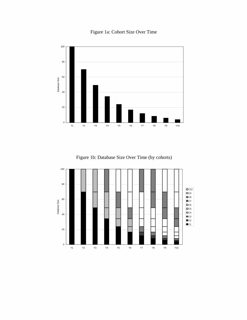
Figure 1a: Cohort Size Over Time

0

20

40

60

80

100

Y1 Y2 Y3 Y4 Y5 Y6 Y7 Y8 Y9 Y10

Dat

abas

e S

ize

Figure 1b: Database Size Over Time (by cohorts)

0

20

40

60

80

100

Y1 Y2 Y3 Y4 Y5 Y6 Y7 Y8 Y9 Y10

Dat

abas

e S

ize

C10

C9

C8

C7

C6

C5

C4

C3

C2

C1

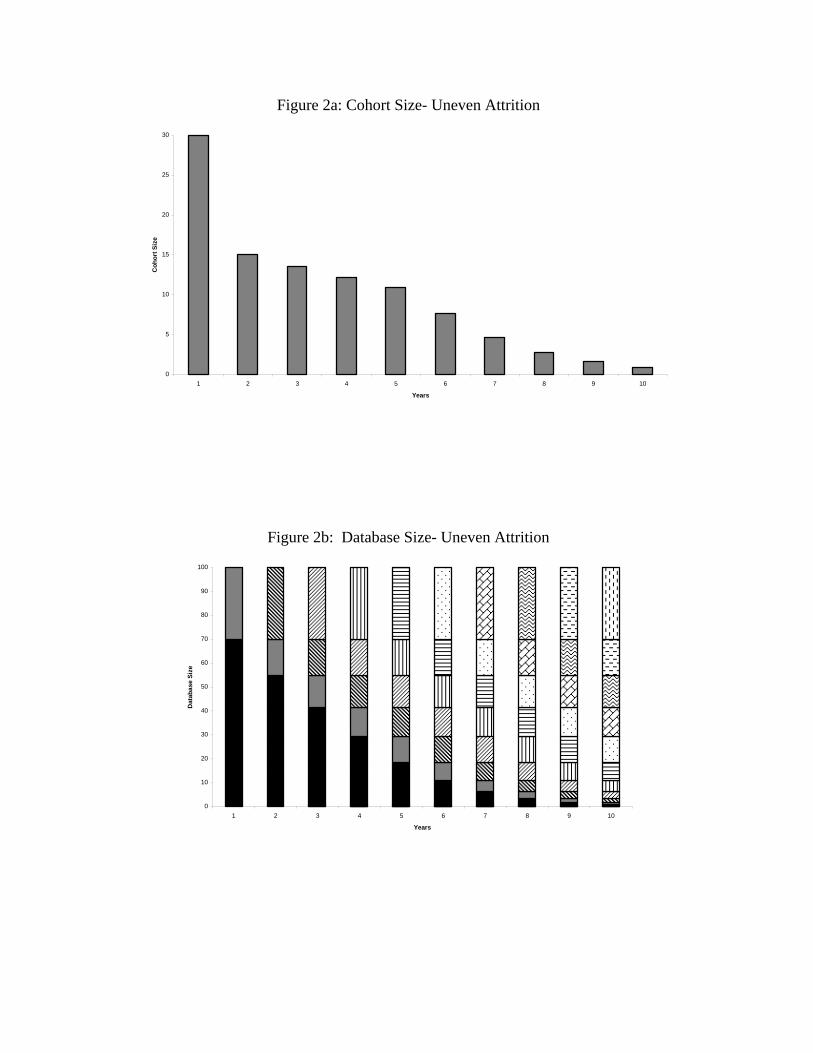
Figure 2a: Cohort Size- Uneven Attrition

0

5

10

15

20

25

30

1 2 3 4 5 6 7 8 9 10

Years

Coh

ort S

ize

Figure 2b: Database Size- Uneven Attrition

0

10

20

30

40

50

60

70

80

90

100

1 2 3 4 5 6 7 8 9 10

Years

Dat

abas

e Si

ze

Moving from Customer Lifetime Value to Customer Equity

Technical Appendix

1. Value of Information

( )A τ is the expected gross revenue realized by the firm for each person to whom it has sent a

communication. This revenue can take on many different forms depending on which type of business is

conducted by the firm. To understand how τ affects A let us look at a concrete example. CDNow uses

its email newsletter to inform its customer of new music CD arrivals in the hope that they will purchase

them. What happens to CDNow if it spaces out the newsletters? On the one hand, if more time elapses,

then CDNow can expect that more new CDs will be released, and thus it is more likely that a CD with

broad appeal is released (which would lead to an increase in A ). On the other hand, information about

CDs is likely to be time sensitive in that the longer CDNow waits, the more likely its customers will have

already purchased the CD promoted by the newsletter (which leads to a decrease in A ).

In more general terms, let us assume that the firm uses an email newsletter to provide its

customers information that might be valuable to them (e.g., the release of Britney Spear’s new album for

CDNow; the release of a new laser printer for Hewlett Packard). This information arrives to the firm on a

continuous basis, but varies in its value to the customer. The arrival process is exponential and the value

of the information is distributed Uniform[0,1]. Once this information is in the possession of the firm, its

value to the customer will decay at an exponential rate until it is sent. Finally, let us assume that for each

communication the firm will pick the one piece of information – out of all the information that it received

since the last communication – that it deems most valuable to its customers.

These assumptions mean the following: (1) the information is generated by a memory-less

process that is not under the control of the marketer; (2) not every piece of information is as valuable to

the customer; (3) the information is time-sensitive; and (4) firms are limited in the length of their

communications. This last assumption may seem arbitrary. Its purpose is to ensure that there are

TA-1

decreasing marginal returns from waiting even when the information is not time sensitive. It can be

justified theoretically by the research on information overload (see Bettman 1979 or Wright 1973), which

shows that consumers can be overwhelmed when they are presented with too much information. It can

also be justified empirically by the fact that three out of the top five reasons people give for un-

subscribing to a newsletter are: the content is irrelevant (55%), poor content (32%), and too long (26%)

(Forrester Research 2001).

The figure below shows a hypothetical example where the firm received 4 pieces of information

I1-I4. In this case, the firm would choose to send information I3 to its customers. The impact of

information decay can be seen in that although I2 was originally more valuable than I4, at τ , I4 has

become more valuable.

The revenue that the firm will be able to extract from the consumer is a function of how valuable

the information is to the consumer. It is natural to assume that the more valuable the information is to the

consumer, the more revenue the firm can generate out of it (i.e., ( )( ) ( )A f Iτ τ= , and ( ) 0f II

∂>

∂). In

Val

ue o

f the

info

rmat

ion

(I)

I4

I1 I2 I3 τ

TA-2

other words, (( ) ( )A f I )τ τ= is the production function of the firm that maps the value of the

information to consumers ( ( )I τ ) into revenue to the firm ( ( )A τ ) via a demand-curve.

Thus, we are interested in the behavior of ( )I τ . This represents the expected value of the most

valuable piece of information arriving in τ periods of time. If the arrival rate for the information is

Poisson of mean μ and the value of the information is Uniform[0,1], then in the absence of information

decay, ( )I τ is the expected value of a Poisson mixture with the order statistics of series of Uniform

draws. For this, note first that the maximum of n random variables with pdf ( )Xf y , and cdf is

distributed as:

( )XF y

[ ] 1( ) ( ) ( )n

nY X Xf y n F y f y−= (TA-1)

Based on this, we note that the maximum of n uniform variables is equal to 1

nn +

. For the uniform

distribution, , . So the expected value of the maximum of the n uniform variables is

given by:

( ) 1Xf y = ( )XF y y=

1 1

11 11

00 0

( ) .[ ] .1 .

[ ( )] . . .1 1

n

n

n nY

n n nY

f y n y n y

nE f y n y y dy n y dy yn n

− −

−

= =

⎡ ⎤⇒ = = = =⎢ ⎥1 n+

+ +⎣ ⎦∫ ∫ (TA-2)

We are interested in the functional form of ( )I τ . One approach to calculating this would be to

compute the expected value of a Poisson mixture with the order statistics of series of Uniform draws. This

can be done in the absence of information decay; however, when information decay is present, the order

statistics cannot be computed for any arbitrary number of draws. And thus one cannot compute the

expected value of the Poisson mixture. Nevertheless, it is possible to derive an expression for ( )I ττ

∂∂

and

from there solve the differential equation to recover ( )I τ . We do so in the next few paragraphs. In this

first derivation, we ignore information decay as it makes the exposition easier to follow.

TA-3

2. No Information Decay

To compute ( )I ττ

∂∂

let us assume that we are at time τ and that we possess information of value ( )I τ .

We can compute the derivate of ( )I τ with respect to τ as:

( )0

( ) (( ) lim t

)E I t IIt

τ τττ Δ →

+ Δ −∂=

∂ Δ. (TA-3)

If we ignore information decay, [ ( )]E I tτ + Δ is given by:

1 ([ ( )] ( )(1 ( )) ( )2

)IE I t I P t P t ττ τ ++ Δ = − Δ + Δ (TA-4)

where,

( )P tΔ is the probability that waiting tΔ will produce a piece of information that is

more valuable than ( )I τ ,

1 (2

)I τ+ is the expected value of the new information conditional on the fact that is better

than ( )I τ .

For a Poisson process, the probability of receiving a new piece of information is tμΔ .i Further,

the probability that the information is more valuable than ( )I τ is (1 ( )I τ− ). Thus, we have:

( )( ) ( )1 ( )[ ( )] ( ) 1 1 ( ) 1 ( )2IE I t I t I t I ττ τ μ τ μ τ +

+ Δ = − Δ − + Δ −

2[ ( )] ( ) ( )(1 )2 2

t tE I t I I tμ μτ τ τ μΔ Δ⇔ +Δ = + − Δ + . (TA-5)

2

0

( ) ( )(1 ) ( )[ ( )] ( ) 2 2lim t

t tI I tE I t It t

Iμ μτ τ μ ττ τΔ →

Δ Δ+ − Δ + −+ Δ −

⇒ =Δ Δ

( )2( ) ( ) 2 ( ) 12

I I Iτ μ τ ττ

∂⇒ = − +

∂ (TA-6)

TA-4

This differential equation characterizes the derivative of the value of the information with respect

to τ . One can use this equation and the knowledge that (0) 0I = to solve the differential equation and

recover the functional form of ( )I τ (see section 2 below):

( ) 2I τττ

μ

=+

(TA-7)

Thus, ( )I τ is a monotonic increasing function that starts at 0 for 0τ = and asymptotes to 1

when τ →∞ . Further:

22I

IIτη

τ μτ∂

= =∂ +

(TA-8)

Hence, Iη is positive, it is at a maximum when 0τ = ( 0 1Iη = ), and it decreases as τ increases

( ). Going back to 0Iη∞ = Aη , our analysis of ( )I τ reveals that Aη is positive but decreases as τ

increases, further 0Aη → when τ →∞ .

3. Information Decay

Let us now assume that once received by the firm, any piece of information decays in its value to the

consumers as time passes. Let ( , )X I tΔ be the value of a piece of information (I) that the firm has sat on

for . If the information decay is exponential in nature, we can write tΔ ( , )X I tΔ as:

( , ) . .tX I t I e λ− ΔΔ =

We can now rewrite (TA-4) as:

1 ( ( ),[ ( )] ( ( ), )(1 ( )) ( )2

)X I tE I t X I t P t P t ττ τ + Δ+ Δ = Δ − Δ + Δ

where,

( ) .(1 ( ( ), ))P t t X I tμ τΔ = Δ − Δ .

Substituting these terms into (TA-5) we now have:

TA-5

2 2[ ( )] ( ) ( ) (1 )2 2

t tt tE I t I e I e tλ λμ μτ τ τ μ− Δ − ΔΔ Δ+ Δ = + − Δ + .

We can now compute the derivate of tI with respect to t:

2 2

2 2

2 2

( ) ( ) (1 ) ( )[ ( )] ( ) 2 2

1 1( ) ( )( ( ) )2 2

1( ) ( )( ))2 2

t t

t t

tt t

t tI e I e tE I t It t

I e I et t

eI e I et

λ λ

λ λ

λλ λ

Iμ μτ τ μτ τ

μ μτ τ μ

μ μτ τ μ

− Δ − Δ

− Δ − Δ

− Δ− Δ − Δ

τΔ Δ+ − Δ + −+ Δ −

=Δ Δ

= + − − +Δ Δ−

= + − +Δ

.

As , , , and 0tΔ → 2 1te λ− Δ → 1te λ− Δ →1te

t

λ

λ− Δ −

→ −Δ

, hence:

2( ) ( ) ( ) ( )2 2

I I Itτ μ μτ μ λ τ∂

= − +∂

+ . (TA-9)

The effect of introducing information decay is, thus, to reduce ( )I ττ

∂∂

. We can compute the point at

which the information asymptotes by looking at the point at which ( ) 0Itτ∂

=∂

:

2

2 2

2

( ) ( ) ( ) 02 2

( ) ( )( )

( ) 2( )

I I

I

I

μ μτ μ λ τ

μ λ μ λ μτ

μ

μ λ λ μλτ

μ

− + + =

+ ± + −⇒ =

+ − +⇒ =

(TA-10)

The minus sign is chosen over the plus sign because ( )I τ cannot be greater than 1. What we see

here is that, in the absence of decay (i.e., 0λ = ), ( )I τ asymptotes to 1; in the presence of decay, ( )I τ

asymptotes to a positive number smaller than one (in the degenerate case where 0μ = , ( )I τ is always

null).

TA-6

4. Solving the differential equation in (TA-9)

To obtain ( )I τ we need to solve the following ODE (TA-9) for ( )I τ :

2( ) ( ) ( ) ( )2 2

I I Iτ μ μτ μ λ ττ

∂= − + +

∂ (TA-11)

which we factorize to obtain:

( ) ( ) ( )2

I d dI Iτ μ μ λ μ λτ ττ μ μ μ μ

⎛ ⎞⎛⎛ ⎞ ⎛∂ + += − + − −⎜ ⎟⎜⎜ ⎟ ⎜∂ ⎝ ⎠ ⎝⎝ ⎠⎝

⎞⎞⎟⎟⎠⎠

(TA-12)

where 2 2d λ μλ= + .

In order to find the general solution, first separate the variables as follows. We put all the terms

involving ( )I τ on the right-hand side. Then we integrate, to get:

1

( ) ( ) ( )2

d dI I dIμ λ μ λ μ dτ τ τμ μ μ μ

−⎛ ⎞⎛ ⎞⎛ ⎞ ⎛ ⎞+ +

− + − − =⎜ ⎟⎜ ⎟⎜ ⎟ ⎜ ⎟⎝ ⎠ ⎝ ⎠⎝ ⎠⎝ ⎠

∫ ∫ τ (TA-13)

Then we re-arrange the left-hand side, given that:

1 1 1 1( )( ) ( ) ( ) ( )x a x b b a x b x a

⎛ ⎞= −⎜ ⎟− − − − −⎝ ⎠

which means we can rewrite (TA-13) as:

111

11

2 ( ) ( ) ( )2

( ) ( ) ( )

d d dI I dI

d d

d

I I dI

μ λ μ λ μ

d d

τ τ τμ μ μ μ μ

μ λ μ λ

τ

τ τ τμ μ μ μ

−−−

−−

⎛ ⎞⎛ ⎞ ⎛ ⎞⎛ ⎞ ⎛ ⎞ ⎛ ⎞− + +⎜ ⎟− − − − + =⎜ ⎟ ⎜ ⎟⎜ ⎟ ⎜ ⎟ ⎜ ⎟⎜ ⎟⎝ ⎠ ⎝ ⎠ ⎝ ⎠⎝ ⎠ ⎝ ⎠⎝ ⎠

⎛ ⎞⎛ ⎞ ⎛ ⎞⎛ ⎞ ⎛ ⎞+ +⎜ ⎟− − − − − + =⎜ ⎟ ⎜ ⎟⎜ ⎟ ⎜ ⎟⎜ ⎟⎝ ⎠ ⎝ ⎠⎝ ⎠ ⎝ ⎠⎝ ⎠

∫ ∫

∫ ∫ τ

(TA-14)

Without the constant, the solution to the left-hand side integrand is (noting that ln( / ) ln( / )a b b a− = :

ln ( )

ln ( )

dI

dI

μ λτμ μ

μ λτμ μ

⎛ ⎞+− +⎜ ⎟⎝⎛ ⎞+

− −⎜ ⎟⎝ ⎠

⎠ (TA-15)

TA-7

With the right-hand side:

ln ( )

ln ( )

dId

dI

μ λτμ μ

τμ λτμ μ

⎛ ⎞+− +⎜ ⎟⎝ ⎠ = +⎛ ⎞+

− −⎜ ⎟⎝ ⎠

c (TA-16)

Then taking exponents of both sides yields:

1 1

( )exp( ), exp( )

( )

dIc d c

dI

μ λτμ μ

τμ λτμ μ

⎛ ⎞+− +⎜ ⎟⎝ ⎠ = =⎛ ⎞+

− −⎜ ⎟⎝ ⎠

c

Solving for ( )I τ :

1

1

1

1

exp( )( )

1 exp( )(1 exp( ))(1 exp( ))

d d c dI

c dc ddc d

μ λ μ λ τμ μ μ μ

ττ

τμ λμ μ τ

⎛ ⎞+ +− − + −⎜ ⎟

⎝ ⎠=− +++

= +−

(TA-17)

Recognizing that at , (0) 0I =

1dcd

λ μλ μ+ +

=+ −

. (TA-18)

Expression (TA-17) is not very user-friendly. A plot if I(t) both in the presence of decay (TA-17),

and in the absence of decay (TA-7), is shown below. As one can see, in the presence of information

decay, the shape of ( )I τ is similar to that when there is no decay; except that it asymptotes to a number

smaller than one. The sign of the first and second order derivatives are preserved. The asymptote point is

given by (TA-10).

TA-8

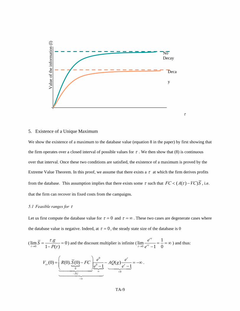
Val

ue o

f the

info

rmat

ion

(I)

No Decay

Deca

y

τ

5. Existence of a Unique Maximum

We show the existence of a maximum to the database value (equation 8 in the paper) by first showing that

the firm operates over a closed interval of possible values for τ . We then show that (8) is continuous

over that interval. Once these two conditions are satisfied, the existence of a maximum is proved by the

Extreme Value Theorem. In this proof, we assume that there exists a τ at which the firm derives profits

from the database. This assumption implies that there exists some τ such that ( ( ) )FC A VC Sτ< − , i.e.

that the firm can recover its fixed costs from the campaigns.

5.1 Feasible ranges for τ

Let us first compute the database value for 0τ = and τ = ∞ . These two cases are degenerate cases where

the database value is negative. Indeed, at 0τ = , the steady state size of the database is 0

(0

.lim 01 ( )

gSPτ

ττ→

=−

= ) and the discount multiplier is infinite (0

1lim1 0

r

r

ee

τ

ττ→= = ∞

−) and thus:

0

00

0

(0) (0). (0) ( )1 1

r

ce r

FC

e eV R S FC AQ ge e

∞ <−

−∞

⎛ ⎞= − −⎜ ⎟⎜ ⎟ − −⎝ ⎠

= −∞ .

TA-9

At τ = ∞ we have another degenerate case, but here it is a case where steady state is never

reached. The firm sends a communication at t=0 and then acquires new names for the rest of eternity

without ever initiating any new communications. Thus, if we assume that 0 0S = , we have

( ) ( )1

r

ce r

eV AQ ge

∞ = −−

.

Given that both Vce(0) and Vce(∞) are negative, and that we assume there exists a τ for which the

database has a positive value, then, by the Intermediate Value Theorem, there exists

min min min: 0 ( ) 0p ceand Vτ τ τ τ< < = and max max max: p ceand V ( ) 0τ τ τ τ< < ∞ = . Thus, the domain over

which the firm operates can be defined by the closed interval [ ]min max,τ τ .

5.2 DBV is continuous over [ ]min max,τ τ

Looking at (C-2 in the paper), we see that the derivative of ( )ceV τ exists everywhere except where

, 1 0re τ − = 0τ = , and ( ). ( ) 0R Sτ τ = . The first two cases occur when 0τ = , the third case occurs

when no money is generated by the communications. Since min 0τ > , the former cannot occur over the

interval [ ]min max,τ τ . Further, since ( ) 0ceV τ ≥ over [ ]min max,τ τ , then ( ). ( )R S Fτ τ ≥ C and thus the

latter cannot occur either.

Since ( )ceV τ is differentiable over the domain [ ]min max,τ τ , it is also continuous over that

domain. Thus, by the Extreme Value Theorem, a maximum exists in the interval. Since 0pτ > , the

maximum is also positive.

5.3 Uniqueness of the Maximum

Let us first rewrite (8) as:

( ) ( ). ( ). ( ) . ( ) ( ). (1)ce

a b c

V R S D FC D AQ g Dτ τ τ τ τ= − − . (TA-19)

where:

TA-10

.

.( )1

r x

r x

eD xe

=−

.

In (TA-19), the third term (c) is independent of τ and can be ignored (see Lemma 2). Thus, we

can show uniqueness of the maximum by showing that the first term (a) has a unique maximum, and that

the second term (b) is a monotonous decreasing function of τ and, thus, the difference of the two terms

has a unique maximum.

i. Unique maximum for a

To prove that the first term has a unique maximum, we look at its second derivative in logs. If the second

derivative is strictly negative, then log(a) has a unique maximum, and thus a also has a unique maximum.

( ) ( ) ( )

22 22

2

0

( ). ( ). ( )

log( ) log ( ) log ( ) log ( )

log( ) ( ) ' ( ) ' ( ) '( ) ( ) ( )

log( ) ( ) ' ( ) ' ( ) ' ( )" ( )" ( )" .( ) ( ) ( ) ( ) ( ) ( )

a R S D

a R S D

a R S DR S D

a R S D R S DR S D R S D

τ τ τ

τ τ τ

τ τ ττ τ τ τ

τ τ τ τ τ ττ τ τ τ τ τ

<

=

= + +

∂= + +

∂

⎛ ⎞⎛ ⎞ ⎛ ⎞∂= − − − + + +⎜ ⎟⎜ ⎟ ⎜ ⎟∂ ⎝ ⎠ ⎝ ⎠⎝ ⎠ τ

Further, we have: ( ) 0, ( ) 0, ( ) 0, ( )" 0, ( )" 0R S D R Dτ τ τ τ τ> > > < < . Thus, a sufficient (but not

necessary) condition for the uniqueness of the maximum is that ( )" 0S τ < . We can reasonably expect

( )S τ to be concave over the feasible domain and, thus, the condition to be satisfied. If not, the necessary

condition for convexity is:

22 2

0

( )" ( ) ' ( ) ' ( ) ' ( )" ( )" .( ) ( ) ( ) ( ) ( ) ( )

S R S D R DS R S D R Dτ τ τ τ τ ττ τ τ τ τ

>

⎛ ⎞⎛ ⎞ ⎛ ⎞< + + − −⎜ ⎟⎜ ⎟ ⎜ ⎟⎝ ⎠ ⎝ ⎠⎝ ⎠ τ

We have:

TA-11

( ) ( )( )( )

22

32

.( )1 ( )

2 1 ' 2 ' 1 "( ) .1

gSP

g P P P P PSP

τττ

τ τττ

=−

− − + −∂⇒ =

∂ −

Thus:

( ) ( )( )( )

2

3

22

2

2 1 ' 2 ' 1 "( )" 1( ) .1

1 ( 1)2 ' 2 ' ( 1) "( 1)

2 ' (1 ) "' .( 1) (1 )

g P P P P PS PS gP

P P P P PP

p P PPP P

τ τττ τ

τ

τ

− − + − −=

−

− −⎡ ⎤= − +⎢ ⎥− ⎣ ⎦−⎡ ⎤= + +⎢ ⎥− −⎣ ⎦

−

Hence, concavity is met if:

( )

22 2

2

22 2

2

2 ' (1 ) " ( ) ' ( ) ' ( ) ' ( )" ( )"'( 1) (1 ) ( ) ( ) ( ) ( ) ( )

( ) ' ( ) ' ( ) ' ( )" ( )" 2 ' (1 )" 1 '( ) ( ) ( ) ( ) ( ) ( 1)

P P P R S D R DPP P R S D R D

R S D R D P PP P PR S D R D P

τ τ τ τ ττ τ τ τ τ

τ τ τ τ ττ τ τ τ τ τ

⎛ ⎞⎛ ⎞ ⎛ ⎞−⎡ ⎤+ + < + + − −⎜ ⎟⎜ ⎟ ⎜ ⎟⎢ ⎥− −⎣ ⎦ ⎝ ⎠ ⎝ ⎠⎝ ⎠

⎛ ⎞⎛ ⎞ ⎛ ⎞ −⎡⇒ < − + + − − − +⎜ ⎟⎜ ⎟ ⎜ ⎟ −⎝ ⎠ ⎝ ⎠⎝ ⎠.

⎡ ⎤⎤⎢ ⎥⎢ ⎥⎣ ⎦⎢ ⎥⎣ ⎦

τ

That is, it is concave as long as P is not too convex.

ii. Monotonicity of b

The fact that b is a monotonously decreasing function of τ can easily be seen by showing that its first

derivative is negative:

2

2

2 .( 1)

r

r

b rFCe

τ

ττ∂

= −∂ −

e

QED

TA-12

6. References

Bettman, James R. (1979), An Information Processing Theory of Consumer Choice, Reading, MA:

Addison-Wesley.

Forrester (2001), “Effective Email Marketing,” The Forrester Report, August.

Mood, Graybill and Boes (1974), Introduction to the Theory of Statistics, McGraw-Hill Publishing

Company.

Wright, Peter L. (1973), “The Cognitive Process Mediating Acceptance of Advertising,” journal of

Marketing Research, 10 (February), 53-62.

i Per Mood, Graybill and Boes, for very small time interval, the probability of one event occurring in a Poisson

process of parameter μ is much larger than the probability of more than one event occurring, and is equal to

tμΔ .

TA-13