Embed Size (px)
Citation preview

1
Moving Towards Improved Basin-level Oil and Gas Inventories and Reconciliation with Measurements
Amnon Bar-Ilan, John Grant, Rajashi Parikh, Ralph Morris
ENVIRON International Corporation, 773 San Marin Drive, Suite 2115, Novato, CA 94998
Garvin Heath, Viktor Diakov National Renewable Energy Laboratory, 15013 Denver West Parkway, Golden, CO 80401
Dan Zimmerle
Colorado State University, Fort Collins, CO 80523
Lee Gribovicz Airstar Consulting, 3570 East 8th St. Casper, WY 82609
ABSTRACT
The Western Regional Air Partnership (WRAP) Phase III emission inventories for oil and gas have been widely distributed and used for inventory, reporting, and air quality modeling in the Rocky Mountain region. We report on the most recent basin for which a WRAP Phase III-type inventory has been developed – the Williston Basin in Montana/North Dakota including the Bakken oil formation. We discuss several innovations that were implemented in this basin including the use of tribal minor new source review (MNSR) data available through Subpart OOOO, and the estimation of oil-production specific source categories in the Bakken formation. We then discuss the comparison of WRAP Phase III inventories with measured inventories, including a case study of inventory analysis relative to measurement data in the Denver-Julesburg (D-J) Basin in Colorado. Inverse modeling was performed and compared to aircraft measurements of volatile organic compound (VOC) fluxes from Weld County in the D-J Basin and determined that inventories were undercounting several key VOC species. This led to identification of potential sources of additional VOC emissions and modification of the inventory. Finally we discuss the implications of these past efforts on a new project sponsored by the US Department of Energy’s National Energy Technology Laboratory and carried out by a large research consortium led by the Colorado School of Mines, the National Renewable Energy Laboratory and the National Oceanic and Atmospheric Administration. The project includes the development of a new emission inventory protocol that enhances and extends prior emission inventories of oil and gas air pollutant emitting sources. INTRODUCTION
Oil and gas exploration and production activities occur extensively throughout the Rocky Mountain States in the United States – which includes the states of New Mexico, Colorado, Utah, Wyoming, Montana and North Dakota. These activities include a large number of processes and equipment which can generate air pollution emissions. Given the scope of these activities, these emissions can contribute significantly to the overall county-level or state-level emissions inventories of these Rocky Mountain States. Individual states have undertaken efforts to develop emissions inventories of oil and gas activities occurring within each state. The Western Regional Air Partnership (WRAP) has sponsored the development of regional inventories for oil and gas, intended to cover multi-state regions in the Western United States. The WRAP inventories were developed in two phases – the Phase I inventory1 which was the first-ever attempt to develop a comprehensive regional inventory of oil and gas activities, and the Phase II inventory2 which included a more detailed analysis of compressor engine and drilling rig emissions. Each of these past projects encountered limitations in the availability of data and the comprehensiveness and accuracy of the inventories they generated. Thus WRAP

2
identified the need for a new, comprehensive inventory of oil and gas activities in the Rocky Mountain States. This led to the development of the Phase III inventories. The Phase III inventory project was begun in 2007, and was a comprehensive inventory of all major oil and gas exploration and production activities, processes and equipment in the Rocky Mountain States. The Phase III project covers criteria pollutants, including nitrogen oxides (NOx), carbon monoxide (CO), volatile organic compounds (VOC), sulfur oxides (SOx) and particulate matter (PM). The inventory considers a base year of 2006, and “midterm” projections to 2012 or 2015. The inventory considers both combustion-generated emissions and those from oil and gas exploration or production processes:
Combustion-generated emissions – includes gas compressor engines, tank and separator heaters, boilers and reboilers in dehydrators and gas sweetening processes, flaring, drilling rig and workover rig engines, and miscellaneous engines (e.g. on-site generators, air compressors, vapor recovery units);
Process emissions – includes flashing and working and breathing losses from condensate and oil tanks, venting emissions from dehydrators and gas sweetening units, fugitive emissions from well site and central facility components, vented emissions from pneumatic devices, vented emissions from pneumatic chemical injection pumps, vented emissions from well completions and recompletions, and vented emissions from well blowdowns.
The Phase III inventory considers all oil and gas exploration and production activities up to the
outlet of a natural gas processing facility, or the inlet to a refinery. This scope is generally consistent with the definition of the “upstream” oil and gas sector, as defined separately from oil refining and natural gas transmission and distribution.3 The Phase III inventory scope does not include on-road and off-road mobile sources associated with exploration and production activity, with the exception of drilling and workover rigs. However these mobile sources have been addressed in a new pilot study for the U.S. Environmental Protection Agency (EPA) that focused on the Piceance Basin in Northwestern Colorado.4
Since the development of the Phase III inventories, these inventories have been regularly updated through projections and further analysis, to a calendar year of 2008 in the WestJump Air Quality Modeling Study (AQMS)5 and to a calendar year of 2011 as part of the Three-State Air Quality Study (3SAQS)6. The inventories have also been used extensively in air quality modeling for predicting photochemical ozone formation and PM concentrations, both for research studies and for State Implementation Plan (SIP) modeling under a regulatory framework7. The EPA has used the WRAP Phase III inventories or their recent projections in the national modeling platform8. Most recently the methodologies developed in the WRAP Phase III inventories have been applied to the development of a comprehensive criteria pollutant inventory for the Williston Basin in Montana and North Dakota with a base year of 2011 under the direction and sponsorship of the Bureau of Land Management (BLM). The methodology and results of this work are presented here, including several key innovations that were applied to the Williston Basin inventory.
In addition, this paper discusses the application of the inventories to regional modeling and comparison of model predictions with recent top-down measurements of VOC flux in an oil and gas basin. A case study is presented of top-down measurements conducted by the National Oceanic and Atmospheric Administration (NOAA) in the Denver-Julesburg (D-J) Basin in North-Central Colorado and its comparison to photochemical ozone modeling conducted for the Denver ozone SIP.
Finally, the limitations of the inventories are discussed in the context of comparison to top-down measurements, the source category limitations of the inventories, data availability and other issues. This has prompted the Department of Energy’s National Energy Technology Laboratory (NETL) to sponsor an ongoing study to improve reconciliation between top-down and bottom-up inventories of oil and gas emissions. The ongoing work is discussed and presented in terms of planned improvements to the inventories and the scope and scale of the NETL study.

3
METHODS
The general methodology for developing the Williston Basin inventory follows that of the Phase III inventories. More detailed presentation of the specific emissions estimation methodologies by source category are presented in the technical report for the study which is available through the WRAP9.
The Williston Basin baseline inventory is developed from a combination of (1) production statistics from a commercially available database; (2) survey data from oil and gas companies; (3) permit data from states and the EPA for larger point-source facilities; and (4) minor source registrations for sources on tribal land from EPA. These four data sources are then compiled to generate the complete baseline inventory for each basin. The tribal minor source data represent a key innovation advanced in this study. Oil and Gas Production Statistics
Oil and gas related activity data across the entire Williston Basin were obtained from the IHS Enerdeq database queried via online interface. The IHS database uses data from each state’s Oil and Gas Conservation Commission (OGCC or equivalent) as sources of information for oil and gas activity. This data is also available directly through database querying tools maintained by the respective agencies, however it was determined that the IHS database is more accurate and complete than these state databases and therefore was chosen as the basis for production statistics for this analysis. Two types of data were queried from the Enerdeq database: production data and well data. Production data includes information relevant to producing wells in the basin while well data includes information relevant to drilling activity (“spuds”) and completions in the basin.
Production data were obtained for all counties in the Williston Basin in the form of IHS “298” format data files. The “298” well data contain information regarding historical oil and gas production. The “298”well data were processed with a PERL script to arrive at a database of by- American Petroleum Institute (API)-number, well type, annual gas production, oil production, and water production with latitude and longitude information.
The API number in the IHS database consists of 14 digits as follows: Digits 1 to 2: state identifier; Digits 3 to 5: county identifier; Digits 6 to 10: borehole identifier; Digits 11 to 12: sidetracks; Digits 13 to 14: event sequence code (recompletions).
Based on the expectation that the first 10 digits, which include geographic and borehole identifiers, would predict unique sets of well head equipment, the unique wells were identified by the first 10 digits of the API number.
Well data were also obtained from the IHS Enerdeq database for the counties that make up the Williston Basin in the form of “297” well data. The “297” well data contain information regarding spuds and completions. The “297”well data were processed with a PERL script to arrive at a database of by-API-number, spud and completion dates with latitude and longitude information. Drilling events in 2011 were identified by indication that the spud occurred within 2011. If the well API number indicated the well was a recompletion, it was not counted as a drilling event, though if the API number indicated the well was a sidetrack, it was counted as a drilling event.
Tables 1 and 2 below show the 2011 baseline production statistics and baseline well count statistics, respectively, for the Williston Basin. Table 1. 2011 production by production type and by county for the Williston Basin (counties without oil and gas production are not shown).
Liquid Hydrocarbon
Production Gas Production
County Condensate
(bbl) Oil
(bbl) Primary Gas
(mcf) Associated Gas
(mcf) Produced
Water (bbl) Carter, MT 0 27,436 49,295 0 139,164 Custer, MT 0 0 60,449 0 0 Daniels, MT 0 3,230 0 0 12,488

4
Liquid Hydrocarbon
Production Gas Production
County Condensate
(bbl) Oil
(bbl) Primary Gas
(mcf) Associated Gas
(mcf) Produced
Water (bbl) Dawson, MT 0 595,113 0 53,615 2,700,813 Fallon, MT 15,418 4,822,211 14,055,984 3,549,143 46,058,213 Garfield, MT 0 13,159 0 1,969 74,713 McCone, MT 0 4,200 0 0 90,419 Prairie, MT 0 63,325 430 0 1,880,916 Richland, MT 31,260 11,962,438 21,204 13,428,072 5,983,761 Roosevelt, MT 0 1,779,002 0 999,229 13,167,825 Sheridan, MT 6,435 1,276,436 1,948 439,261 12,952,771 Valley, MT 0 100,412 1,539,084 8,221 1,002,778 Wibaux, MT 0 741,512 221,939 229,797 12,295,410 Billings, ND 7,054 3,830,377 25,874 4,102,338 22,306,981 Bottineau, ND 36,240 1,750,108 2,952 77,376 37,632,266 Bowman, ND 1,866,510 8,018,738 4,570,444 7,945,295 33,665,670 Burke, ND 16,780 2,235,526 40,185 3,196,199 7,074,419 Divide, ND 38,855 5,186,853 52,420 6,021,999 5,948,983 Dunn, ND 154,372 22,268,833 126,213 15,258,523 12,260,749 Golden Valley, ND 0 652,781 0 498,881 2,417,409 McHenry, ND 0 25,849 0 0 513,965 McKenzie , ND 843,889 29,044,894 2,897,188 41,054,821 21,427,508 McLean, ND 0 747,001 0 316,753 355,773 Mercer, ND 0 2,111 0 0 10,598 Mountrail, ND 123,231 50,959,389 71,989 34,121,971 18,254,096 Renville, ND 44,189 810,957 0 100,171 9,950,411 Slope, ND 254,656 307,887 82,364 518,533 1,213,648 Stark, ND 0 2,344,297 0 1,757,258 10,005,696 Ward, ND 0 38,845 0 11,132 570,370 Williams, ND 606,902 20,076,648 3,607,091 29,101,957 26,750,917 Harding, SD 28,053 1,586,475 1,295,351 11,155,586 3,979,830 Total 4,073,844 171,276,043 28,722,404 173,948,100 310,698,560
Table 2. 2011 active well counts and spuds counts by county for the Williston Basin (counties without oil and gas production are not shown). Well Count
Spud Count County Gas Wells Oil Wells Carter, MT 17 1 0 Custer, MT 3 0 0 Daniels, MT 0 2 0 Dawson, MT 0 62 2 Fallon, MT 982 495 2 Garfield, MT 0 12 1 McCone, MT 0 7 0 Prairie, MT 1 12 0 Richland, MT 4 995 34 Roosevelt, MT 0 206 29 Sheridan, MT 1 209 9 Valley, MT 149 41 3 Wibaux, MT 32 81 0 Billings, ND 3 460 31 Bottineau, ND 5 533 12 Bowman, ND 212 329 4 Burke, ND 5 433 47 Divide, ND 5 275 95 Dunn, ND 10 701 220 Golden Valley, ND 0 69 7 McHenry, ND 0 17 0

5
Well Count Spud Count County Gas Wells Oil Wells
McKenzie , ND 46 1,231 353 McLean, ND 0 29 14 Mercer, ND 0 1 0 Mountrail, ND 4 1,124 336 Renville, ND 6 284 5 Slope, ND 5 13 1 Stark, ND 0 102 35 Ward, ND 0 16 0 Williams, ND 38 800 306 Harding, SD 99 136 10 Total 1,627 8,676 1,556
The Williston Basin, unlike all other Rocky Mountain region basins, is characterized by high
levels of crude oil production primarily from the Bakken Shale formation. In 2013, the state of North Dakota was ranked the second highest crude oil producer in the fifty United States due almost entirely to the production in the Bakken10. The Williston Basin is not a large producer of either condensate or natural gas relative to other Rocky Mountain basins and has far fewer primary gas wells than oil wells (by a factor of approximately 5.3 to 1). The vast majority of gas produced in the basin is in the form of associated gas (or casinghead gas) produced as a byproduct from primary oil wells. The majority of this gas is captured and processed for sale, but a significant fraction is not captured due to lack of infrastructure and must instead be flared. This issue is discussed in greater detail below.
Temporal and Geographic Scope
This inventory considers a base year of 2011 for purposes of estimating emissions. All base year
well count and production data for the basin obtained from the IHS database were for the calendar year 2011 and data gathered from a number of sources on emissions and equipment were also for calendar year 2011. Emissions from all source categories are assumed to be uniformly distributed throughout the year except for heaters and pneumatic pumps, which are assigned seasonality fractions as they are typically used primarily in winter.
The geographic scope of this inventory is the Williston Basin in Northeastern Montana, North Dakota, and including a small portion of Northwestern South Dakota. For the purposes of this study, the boundaries for the Williston Basin were modified from those of the US Geological Survey (USGS)11 to wholly include Carter, Custer, Daniels, Dawson, Fallon, Garfield, McCone, Prairie, Richland, Roosevelt, Sheridan, Valley, and Wibaux Counties in Montana; Butte and Harding Counties in South Dakota; and all counties in North Dakota. For purposes of this report, only those counties in North Dakota with some oil and gas activity or midstream sources were included, consisting of Barnes, Billings, Bottineau, Bowman, Burke, Burleigh, Divide, Dunn, Golden Valley, McHenry, McIntosh, McKenzie, McLean, Mercer, Morton, Mountrail, Renville, Slope, Stark, Stutsman, Ward and Williams Counties in North Dakota. The geographic scope of the analysis also considers activities by mineral estate ownership: BLM, United States Forest Service (USFS), Bureau of Indian Affairs (BIA) and state or private fee land.
Figure 1 and Figure 2 show the boundaries of the Williston Basin, with the 2011 well locations extracted from the IHS database overlaid. Figure 1 presents wells by type and Figure 2 presents wells by mineral designation. A key innovation in this study was the determination of mineral ownership and assigning of production and well surrogates to mineral ownership designations. This allowed for the emission inventory to be apportioned by mineral ownership designations, which provides regulatory agencies critical data on the fractions of emissions associated with each agency’s jurisdiction. Mineral ownership was determined by working closely with BLM and other federal agencies to tag wells by API number for which the mineral ownership designation was BLM, USFS and BIA. All other wells were

6
assumed to be state/private/fee land. Production associated with those wells was then obtained through the IHS database analysis described in more detail below.
Figure 1. 2011 oil and gas well locations by well type within the Williston Basin.

7
Figure 2. 2011 oil and gas well locations by mineral designation within the Williston Basin.
2011 Midstream Sources
Permitted midstream sources in the Williston Basin analysis refer to three types of sources for which data was gathered: (1) Title V or major sources in use in midstream, gas gathering applications from permit data from the Montana Department of Environmental Quality (MTDEQ); (2) Title V or major sources in use in midstream applications from NDDOH (North Dakota Department of Health); and (3) Part 71 major sources on tribal land from US EPA Region 8. The three source types are described below. In general, these permitted sources were used to supplement the emissions associated with well-site sources which were derived from survey data and tribal minor source registrations. Most permitted emissions used in this inventory were for midstream facilities which were not included in the exploration and production (E&P) sector surveys described in the next section. Although the MTDEQ and NDDOH register production-site equipment, this study used the detailed survey of operators to estimate emissions from these sources rather than permit data for individual production sites due to the availability of the data and the resources available for processing this data.
Permit Data for Midstream Facilities from State Agencies
Similar to the WRAP Phase III emissions inventories, midstream companies were generally not
participants in the survey process conducted in the Williston Basin, with the exception of some gas and oil producers who may also own and operate midstream facilities. Because NDDOH and MTDEQ permit large midstream sources on non-tribal land in each state respectively, it was determined that these permit databases would be the most comprehensive source of data on midstream facilities such as gas plants, compressor stations and associated equipment. Requests were made to the MTDEQ and NDDOH to query their database of permitted facilities to identify midstream oil and gas sources in the Williston Basin using a combination of NAICS (SIC) and SCC codes corresponding to onshore oil and gas

8
sources. This query was focused on facilities and to the extent possible excluded production sites. It is noted that both NDDOH and MTDEQ require registration of production sites including registration of equipment at the sites, but discussions with both agencies indicated that this information was not considered readily available for use in the inventory. Permit Data from EPA Region 8
Title V and Part 71 permits were requested from EPA Region 8 covering the Williston Basin,
primarily for the Fort Berthold and Fort Peck Indian Reservations. Data provided by EPA indicated only a single source in the Fort Peck Indian Reservation meeting the Title V emission thresholds.
Tribal minor source registration emissions were requested from EPA Region 8 covering the Williston Basin, primarily for the Fort Berthold and Fort Peck Indian Reservations. Data provided by EPA indicated eleven compressor stations that did not meet Title V emission threshold, but were reported under EPA’s minor source program. Well Site Sources
Emissions from well site sources were estimated based primarily on two sources of data. A survey effort was conducted to develop basin-wide representative data for well site emission sources. Additionally, tribal minor source well site registrations were obtained from EPA for the Fort Berthold Indian Reservation which allowed for compilation of representative well site data specific to the Fort Berthold Indian Reservation for select well site emission sources. Tribal minor source well site registrations were not obtained from EPA for the Fort Peck Indian Reservation due to the small number of well site registrations that were available for that reservation.
Detailed inventory methodologies for each of the source categories are presented in Section 4.0. Emission estimates were generally made by extending representative emissions per well or per unit of production developed from the survey and tribal minor source data to the entire basin by scaling by the appropriate oil and gas surrogate. Similarly, emissions by mineral designation were estimated by scaling basin-wide emissions by the oil and gas activity surrogate appropriate to each source category. Surveyed Sources
A survey spreadsheet was forwarded to participating operators in the Williston Basin. The
spreadsheet contained requests for specific data related to one of the following 23 source categories: Drill Rigs Fracing Engines Completion Engines Initial Completion Venting Oil and Condensate Tanks Well Truck Loading Artificial Lift Engines Casinghead Flaring Well-site Fugitive Components Heaters Pneumatic Devices Pneumatic Pumps Dehydrators Workover Rigs Refracing Engines Recompletion Venting Other Flaring

9
Miscellaneous Engines Well Blowdown (liquids unloading) Wellsite Compressor Engines Compressor Start-ups and Shutdown Water Tanks Water Disposal Pits
The companies participating in the survey process for the Williston Basin represented
approximately 46% of well ownership in the basin, 70% of gas production in the basin, and 58% of oil production in the basin. Company participation is significantly higher than in the WRAP Phase III Williston Basin Emission Inventory12 for which the companies participating in the survey process represented approximately 20% of well ownership in the basin, 30% of gas production in the basin, and 33% of oil production in the basin. The percentage of oil and gas activity that was captured in the survey process allow for good representation of oil and gas operations in the basin.
Insufficient survey data was obtained to estimate emissions for certain source categories. These source categories were therefore excluded from the study and include amine units, CBM pump engines, truck loading at gas and natural gas liquid (NGL) processing plants, water disposal pits, and saltwater disposal engines. Finally, potential fugitive emissions from oil and gas pipelines from well heads to the main compressor stations were not estimated, consistent with the previous WRAP Phase III study12. Insufficient data was available on the components of pipelines or the complete extent of pipelines to tractably estimate basin-wide pipeline fugitive emissions.
It should be noted that the emission estimates calculated for survey-based sources rely on data that is not as rigorously documented as permitted sources. Much of the data provided for these sources is based upon estimates and extrapolation from the survey responses. However the level of detail of the surveys and the extent of participation in the survey effort allow for emissions estimates of survey-based sources which are a significant improvement over previous emission inventory efforts for the Williston Basin.
For emissions from those source categories that relied on estimates of volume of gas vented or leaked, such as tank flashing, well blowdowns, completions, and fugitive emissions, gas composition analyses were requested from all participating companies for gas produced from oil wells (i.e. casinghead or associated gas), gas produced from gas wells (primary gas), and flash gas associated with oil tanks. These composition analyses were averaged to derive basin-wide gas composition averages for oil wells by associated gas production, for gas wells by primary gas production, and for oil tank flash gas based on oil production. The average composition analyses were used to determine the average basin-wide VOC volume and mass fractions of the vented gas by type (i.e. associated gas, primary gas, and oil tank flash gas). It is noted that due to lack of survey data, condensate tank flash gas compositions were taken from the Phase III study12.
Survey data was aggregated together at the basin-wide level to maintain the confidentiality of each company’s data. Survey data was aggregated across all operators by the weighted average contribution of each company’s data using the surrogate as the weighting factor. This methodology allows each company’s survey data to impact the emissions from each source category in proportion to the company’s ownership of the surrogate assigned to each category.
Tribal Minor Source Registrations
EPA promulgated the Indian Country Minor New Source Review Rule in 2011 and has
subsequently made a number of revisions to this rulemaking. The rule requires registration of existing and new minor sources on tribal land. Minor sources are defined in attainment areas as those sources which do not meet major permitting thresholds with the potential to emit more than:
10 tons per year of carbon monoxide (CO), nitrogen oxides (NOx), sulfur dioxide (SO2), or particulate matter (PM), or

10
Five tons per year of volatile organic compounds (VOCs), or Five tons per year of particulate matter less than 10 microns (PM10), or Three tons per year of particulate matter less than 2.5 microns (PM2.5), or 0.1 tons per year of lead, or One ton per year of flourides, or Two tons per year of hydrogen sulfide (H2S)
In the development of the Williston Basin emission inventory, minor source permitted emissions
summary data, inclusive of both midstream (i.e., compressor station) and well site emissions, were provided by EPA for two tribal reservations within the boundaries of the Williston basin, the FBIR and the Fort Peck Indian Reservation. Midstream permitted source (i.e., compressor station) emissions from the tribal minor source emissions data were incorporated into the draft Williston Basin emission inventory. The tribal minor source emissions summary data also included a significant amount of well site emissions on the FBIR. Subsequent follow-up with EPA and analysis of well site permit registrations indicated the value of analysis of the tribal well site data and the potential for incorporation of this well site data into the Williston Basin emission inventories. Well site emissions from minor source registrations provided by EPA indicated a significant amount of well site emissions for the FBIR, however, well site emissions from Fort Peck minor source registrations were very small. The relatively small amount of well site emissions on the Fort Peck Indian Reservation is not unexpected given that the magnitude of oil production on the Fort Peck Indian Reservation is only 1% of the oil production on the FBIR. The focus of this analysis is the FBIR well site minor source registrations; Fort Peck well site minor registrations were not analyzed.
Tribal minor source registration data was obtained for seven companies representing 73% of oil production, 74% of gas production, and 69% of active well count on the Fort Berthold Indian Reservation according to the IHS Enerdeq database . This is a large percentage of oil and gas activity on the Fort Berthold Indian Reservation which made it possible to obtain a reasonable representation of oil and gas operations on the Fort Berthold Indian Reservation. Analysis of the well site registrations allowed for estimation of representative emission source inputs for use in developing Fort Berthold area emissions for the following categories:
Artificial Lift Engines Compressor Engines Well-Site Fugitive Components Heaters Miscellaneous Engines Oil Tanks Truck Loading of Oil Water Tanks
For source categories that are not listed above, all Fort Berthold Indian Reservation well site
emissions were estimated based on the basin-wide input factors which were developed primarily based on operator surveys. Similarly, all well site emissions outside of the Fort Berthold Indian Reservation were also based on the basin-wide input factors which were developed primarily from operator surveys.
For well site source categories that are available in the tribal minor source registrations (listed in Table 3 below), emission inventory input factors based on the minor source registrations were compiled. The tribal well site input factor data – equipment, process-related data, gas compositions, emission factors, etc. – were compiled for each operator by aggregating across all of each operator’s registrations based on the associated oil and gas activity statistic surrogate from each registration to compile operator average input factors.

11
Table 3. Percent of oil and gas surrogate for each source category for which emissions data was available from Fort Berthold Tribal MNSR data.
Inventory Source Category Oil and Gas Surrogate Surrogate Percent Coverage Artificial Lift Engines** Oil Production 58% Casinghead Gas Associated Gas Production 48% Wellhead Compressor Engines Active Well Count 59% Fugitives Active Well Count 46% Miscellaneous Engines Active Well Count 59% Water Tanks Water Production 22% Heaters Active Well Count 69% Oil Tank Oil Production 71% Truck Loading of Oil Oil Production 71% Natural Gas Composition1 Gas Production 39% Flash Gas Composition1 Oil Production 24%
Operator average input factors for each source category were aggregated across all operators by
the weighted average contribution of each company’s well site registration data using the surrogate as the weighting factor. This methodology allows each company’s well site registration data to impact the emissions from that source category in proportion to the company’s ownership of the surrogate assigned to that category.
The end result of this task is the representative data needed to calculate emissions for each source category representing aggregated tribal well site data. These representative data are shown below in Table 4.
Table 4. Representative well site emissions inputs based on tribal MNSR data mining.
Parameter
Fort Berthold EPA Minor Tribal
Average Data
Williston Basin Survey Producer
Data Unit Oil Tank
Uncontrolled VOC Emission Factor 5.4 5.6 lb/bbl Uncontrolled Flashing Emission Factor 66 68 scf/bbl Fraction of Production Controlled Via Flare 0% 70% - Fraction of Production Controlled Via VRUs 0% 13% - Fraction of Production Controlled Via Enclosed Combustor
100% 6% -
Casinghead Gas Fraction of Gas Flared 85% 25% - Heating Value 1504 1571 btu/scf Flaring control efficiency 97% 90% -
Heaters No. of Heaters per Well 0.98 0.55 count Heater Rating 0.68 0.61 Mmbtu/hr Annual Heater Usage 8760 8309 hr Heater Cycling (fraction of the time the heater is doing work when it is turned on)
100% 98% -
Heating Value 1459 1590 btu/scf Truck Loading
Fraction of Total Oil Production Sent Directly to Pipeline, Not Subject to Well site Loading
54% 31% -
True vapor pressure of liquid loaded 2.25 2.39 psi Temperature of Liquid Loaded 529 515 °R Molecular Weight of Liquid Loaded 46.7 50.0 lb/lb-mole Mode of Operation 100%
submerged loading: dedicated normal
68% - Submerged Loading of a Clean
cargo tank
-

12
Parameter
Fort Berthold EPA Minor Tribal
Average Data
Williston Basin Survey Producer
Data Unit service 32% - submerged
loading: dedicated vapor balance
service Saturation Factor for submerged loading: dedicated normal service
0.66 0.73 -
Fugitives GAS DEVICES Valves Gas 34 28 count pump seals Gas 0 0 count others (please provide description) Gas 1 0 count Connectors Gas 188 95 count Flanges Gas 19 23 count open-ended lines Gas 0 3 count non-GAS DEVICES Valves Heavy Oil 0 0 count Valves Light Oil 29 19 count Valves Water/Oil 7 3 count pump seals Heavy Oil 0 0 count pump seals Light Oil 0 1 count pump seals Water/Oil 1 0 count others (please provide description) Heavy Oil 0 0 count others (please provide description) Light Oil 0 0 count others (please provide description) Water/Oil 1 0 count Connectors Heavy Oil 0 0 count Connectors Light Oil 97 35 count Connectors Water/Oil 43 3 count Flanges Heavy Oil 0 0 count Flanges Light Oil 33 37 count Flanges Water/Oil 2 1 count open-ended lines Heavy Oil 0 0 count open-ended lines Light Oil 1 0 count open-ended lines Water/Oil 0 0 count
Wellhead Compressor Engines Fuel Type Natural Gas Natural Gas - Engine Rated Power 244 408 HP No. of Engines per Well 0.26 0.001 count Hours of operation 8760 8760 hours/year NOx 1.24 2.00 g/hp-hr VOC 0.63 1.00 g/hp-hr CO 2.36 4.00 g/hp-hr SO2 0.00 0.00 g/hp-hr PM 0.09 0.04 g/hp-hr
Misc. Engines – Pump Fuel Type Gasoline Gasoline - Engine Rated Power 8 8 Hp No. of Engines per Well 0.34 0.06 Count Hours of operation 1820 683 hours/year NOx 5.00 3.60 g/hp-hr VOC 7.01 6.12 g/hp-hr CO 3.16 284.57 g/hp-hr SO2 0.27 0.03 g/hp-hr PM 0.32 0.12 g/hp-hr

13
Parameter
Fort Berthold EPA Minor Tribal
Average Data
Williston Basin Survey Producer
Data Unit Misc. Engine –Generator
Fuel Type Diesel Diesel - Engine Rated Power 181 211 HP No.of Engines per Well 0.12 0.17 Count Hours of operation 8021 5735 hours/year NOx 3.77 2.98 g/hp-hr VOC 0.68 0.21 g/hp-hr CO 2.43 2.89 g/hp-hr SO2 0.93 0.00 g/hp-hr PM 0.21 0.21 g/hp-hr
Misc. Engine - Other –NG Fuel Type Natural Gas Natural Gas - Engine Rated Power 250 400 HP No.of Engines per Well 0.07 0.001 Count Hours of operation 8760 8760 hours/year NOx 1.79 2.00 g/hp-hr VOC 0.49 1.00 g/hp-hr CO 1.41 0.50 g/hp-hr SO2 0.00 0.00 g/hp-hr PM 0.09 0.04 g/hp-hr
Artificial Lift Engines Fuel Type Natural Gas Natural Gas - Engine Rated Power 80 70 HP No.of Engines per Well 0.02 0.22 Count Hours of operation 8760 8538 hours/year NOx 25.85 4.46 g/hp-hr VOC 0.98 1.09 g/hp-hr CO 3.14 2.29 g/hp-hr SO2 0.00 0.00 g/hp-hr PM 0.08 0.18 g/hp-hr Fraction of Engines Electric unknown 17% -
Water Tank VOC Emission Factor 0.25 0.05 lb/bbl Fraction of Production Controlled 100% 63.73% - Volume of Gas Flared Not available 0.15 MCF/bbl
Natural Gas Composition Analysis Gas MW 28.06 28.52 g/mol VOC Fraction (molar) 23% 23% - VOC/TOC (weight) 46% 45% - VOC MW 51.96 53.77 g/mol VOC Fraction (weight) 46% 43% - CH4 Fraction (weight) 28% 30% - CO2 Fraction (weight) 1% 1% - Heating Value 1504 1571 btu/scf
Flash Gas Composition Analysis Gas MW 65.52 40.23 g/mol VOC Fraction (molar) 79% 55% - VOC/TOC (weight) 92% 73% - VOC MW 76.60 52.56 g/mol VOC Fraction (weight) 92% 72% - CH4 Fraction (weight) 2% 7% - CO2 Fraction (weight) 0.1% 1% - Heating Value 2367 2092 btu/scf

14
Emission Estimation Methodologies
For each survey-based or tribal MNSR-based source category for well-site emissions, a set of methodologies was used to estimate emissions from these sources for the fraction of activity represented by responding companies or by the tribal MNSR data that was used. These methodologies follow the WRAP Phase III methodologies and were described in detail in a technical report for the Williston inventory9.
Two categories were considered in detail that were not in previous WRAP inventories: (1) casinghead gas flaring and capture; and (2) oil loading at rail terminals. These two sources are unique to the Bakken formation among the Rocky Mountain basins in being significant source categories. The Bakken is characterized by substantial amounts of casinghead gas production in a region that historically has not had the infrastructure for capturing, processing and selling this gas. Operators in the Bakken have made progress in building such infrastructure, but there remains a fraction of casinghead gas production that cannot be captured and must be flared in pit flares. Similarly, the boom in oil production has not matched the infrastructure for transferring the crude oil to refineries and other end destinations. This has led to an increase in the use of rail terminals in which oil is loaded into tanker cars and moved by rail to the next destinations. These two methodologies are described in more detail below.
Casinghead Gas Capture and Flaring
Casinghead gas venting and flaring emissions were estimated based on survey-based data and
data available from the North Dakota Oil and Gas Commission (NDOGC). VOC emissions result from any casinghead gas that is vented to the atmosphere as well as from casinghead gas that is flared. According to operator surveys, less than 0.3% of casinghead gas is vented. NDOGC estimates indicated that in 2011, 63% of produced gas was sold; it was conservatively assumed that any gas not sold was flared, hence 37% of casinghead gas was assumed to be flared. Some casinghead gas is expected to be used at the well site to power gas-fired equipment such as heaters or well site engines, or in other applications such as the generation of electricity or the capture of heavier hydrocarbons. However, data was not available to adequately characterize the percentage of gas that is used in such applications; hence all casinghead gas not sold was conservatively assumed to be flared. Further study to quantify the extent of alternative casinghead gas usage would allow for additional refinement of casinghead gas flaring emissions.
Casinghead gas flaring was assumed to occur only for Bakken Formation Counties, which is consistent with a majority of associated gas production in the Williston Basin occurring in the Bakken Formation Counties. A flare destruction efficiency of 90% was assumed.
VOC emission from casinghead gas were estimated per Equation 1.
(Equation 1) FFCYTR
MW1000VPE effVOC
VOCTOTALvented
gheadca
11
,
sin
where: Ecasinghead is the VOC emissions from casinghead gas [lb/year] Vvented,TOTAL is the total volume of casinghead gas that is vented [mscf/year] MWVOC is the molecular weight of the VOC [lb/lb-mol] R is the universal gas constant [scf-atm/K-lb-mol] YVOC is the volume fraction of VOC in the vented gas Ceff is the flaring control efficiency F is the fraction of vented volume that is flared
1,000 is the volume units conversion factor [scf/mscf] T is the temperature [K]

15
P is the pressure in [atm] The conversion from volume of gas vented to mass of VOC produced was evaluated at standard
temperature and pressure. The total VOC emissions from all casinghead gas venting and flaring as described in Equation 1
represent basin-wide casinghead VOC emissions. County-level emissions from casinghead gas were estimated by allocating the total basin-wide casinghead gas emissions into each county according to the fraction of 2011 associated gas production from oil wells occurring in that county. Emissions by mineral designation were estimated in each county by allocating the county total emissions into each mineral designation according to the fraction of total 2011 associated gas production from oil wells that occurred in each mineral designation in that county.
Rail Loading of Crude Oil
Based on information provided by NDDOH13 29 million barrels of oil was estimated to be
loaded onto rail in 2011 in Bakken Formation counties, with 53% of the loading emissions accounted for in the NDDOH provided midstream data; therefore 47% of rail loading emissions were estimated as an area source using the methodology described here. Rail truck loading emissions were estimated based on loading losses per EPA AP-42, Section 5.2 methodology combined with the estimates of volume loaded to rail and controlled by flare. The loading loss rate was estimated based on EPA AP-42, Section 5.2 methodology, following Equation 2 below:
(Equation 2)
T
MVSL 46.12
where:
L is the loading loss rate [lb/1000gal] S is the saturation factor taken from AP-42 default values based on operating mode V is the true vapor pressure of liquid loaded [psia] M is the molecular weight of the vapor [lb/lb-mole] T is the temperature of the bulk liquid [oR]
Total rail loading emissions were then estimated by combining the calculated loading loss rate
with the volume of oil loaded to rail as shown in Equation 3:
(Equation 3) 1000
42 PLEloading
where:
Eloading is the rail loading emissions [lb/year] L is the loading loss rate [lb/1000gal] P is the volume of oil loaded to rail not including the volume loaded to rail that is accounted for in midstream source emissions [bbl/yr] 42 is the volume-units conversion factor [gal/bbl] 1,000 is the volume-units conversion factor [gal/1000gal]
The basic emission estimation methodology described in Equations 2 and 3 above accounts for
total basin-wide emissions from rail loading losses. County-level emissions were estimated by allocating the total basin-wide rail loading emissions
into each Bakken Formation County according to the fraction of oil production in each county. Rail loading was assumed to be limited to Bakken Formation Counties. Emissions by mineral designation
16
were estimated in each county by allocating the county total emissions into each mineral designation according to the fraction of total 2011 oil production that occurred in each mineral designation in that county.
General Compilation Methodology
The survey and permit data were compiled in several steps to generate the baseline 2011
inventory. A set of surrogates were applied to each survey-based source category for which survey data was compiled, and similar surrogates were applied to the tribal MNSR input data for those categories in Table 3. The surrogates represented different oil and gas production statistics, such as primary gas production, casinghead gas production, oil production, condensate production, oil or gas well counts and spud (drilling event) counts. For each source category, the total value of the surrogate represented by all responding oil and gas companies whose data contributed to the survey was compared to the total value of the surrogate in the basin (or to the total value of the surrogate in the FBIR for tribal data). A scaling factor was developed, which was the ratio of the total value of the surrogate in the basin to that represented by the combined survey responses. The scaling factor was used to grow the total emissions for survey and tribal MNSR sources for each source category from the survey data to the basin-wide or tribal-wide emissions respectively. This was done because the survey respondents did not represent all activity in the basin.
Following this, the emissions from permitted sources were added to the emissions from the survey-based sources. The permitted sources were treated as point sources, since the exact locations of these sources were known. The resulting emissions inventory represented the total inventory. The surrogates for each source category were then used to scale the inventory down to the county level, such that the final inventories were reported on a county basis. The scaling factors for the county-level emissions estimates were the ratio of a surrogate’s value in a single county to that of the entire basin. A similar analysis was conducted for tribal versus non-tribal land. An analysis was conducted to determine the values of surrogates within tribal land in the basin, as opposed to non-tribal land. A similar scaling was then conducted on the total inventory for the basin to determine the tribal portion of the inventory. More details on this methodology are available in the references9. INVENTORY RESULTS Results from the combined permitted sources and the combined surveyed sources are presented below for the entire Williston Basin as a series of pie charts and bar graphs including county-level emissions, basin-wide emissions and emissions on tribal and non-tribal land. The quantitative emissions summaries are presented in Table 5. It should be noted that all figures showing county-level emissions only include those counties representing 1% or greater of the total emissions in the basin. A complete list of emissions for all counties is included in the summary emissions spreadsheets that accompany this report.
Figure 3 shows NOx emissions by county and source category in the Williston Basin. Figure 3 shows that NOx emissions are concentrated in McKenzie, Mountrail, Williams, and Dunn Counties in North Dakota, and to a lesser extent in Richland and Fallon Counties in Montana. These counties represent the core Bakken Formation area, with the exception of Fallon County in the Cedar Creek Anticline. Figure 4 shows NOx emissions by mineral designation in the Williston Basin. 77% of NOx emissions are from private/state fee mineral estate with less than 12% of NOx emissions from any other single mineral estate.
Figure 5 shows that VOC emissions are also concentrated in McKenzie, Mountrail, Williams, and Dunn Counties in the core of the Bakken area of North Dakota, and to a lesser extent in Richland and Fallon Counties in Montana. There are also significant VOC emissions in Bowman County in the Cedar Creek Anticline. 78% of VOC emissions are from private/state fee mineral estate with less than 10% of VOC emissions from any other single mineral estate.

17
Figure 7 shows VOC emissions by mineral designation. Figure 8 shows that VOC emissions from casinghead gas, oil tank flashing, and pneumatic devices are the largest contributors to basin-wide VOC emissions, accounting for approximately 81% of the basin-wide VOC emissions in the Williston Basin in 2011. Condensate tank flashing represents an additional 9% of basin-wide VOC emissions in the Williston Basin in 2011.
Figure 3. 2011 NOx emissions by source category and by county in the Williston Basin.
Figure 4. 2011 NOx emissions by mineral designation in the Williston Basin.
0
1000
2000
3000
4000
5000
6000
7000
8000
NO
x E
mis
sio
ns (
ton
s/y
ear)
County
Other Categories
Water Tank Flaring
Heaters
Initial completion Flaring
Fracing
Casinghead Gas Venting
Oil Well Truck Loading
Oil Tank
Condensate tank
Artificial Lift
Miscellaneous engines
Survey-based Fugitives
Venting - initialcompletionsPneumatic pumps
Pneumatic devices
Casinghead Gas Flaring
Drill rigs
Compressor engines
Chart represents by source category NOx emissions for only those counties which contribute greater than 1% of NOx basinwide emissions.
0
5,000
10,000
15,000
20,000
25,000
BLM Tribal Private/State U.S. Forest Service
NO
x E
mis
sio
ns (
ton
s/y
ea
r)
South Dakota- Total
North Dakota- Total
Montana - Total

18
Figure 5. 2011 VOC emissions by source category and by county in the Williston Basin.
Figure 6. 2011 VOC emissions by mineral designation in the Williston Basin.
0
10000
20000
30000
40000
50000
60000
70000V
OC
Em
issio
ns (
ton
s/y
ea
r)
County
Other Categories
Water Tank Flaring
Heaters
Initial completionFlaringFracing
Casinghead GasVentingOil Well Truck Loading
Oil Tank
Condensate tank
Artificial Lift
Miscellaneous engines
Survey-based Fugitives
Venting - initialcompletionsPneumatic pumps
Pneumatic devices
Casinghead GasFlaringDrill rigs
Compressor engines
Chart represents by source category VOC emissions for only those counties which contribute greater than 1% of VOC basinwide emissions.
0
50,000
100,000
150,000
200,000
250,000
BLM Tribal Private/State U.S. Forest Service
VO
C E
mis
sio
ns
(to
ns
/ye
ar)
South Dakota- Total
North Dakota- Total
Montana - Total

19
Figure 7. 2011 Williston Basin NOx emissions proportional contributions by source category.
Figure 8. 2011 Williston Basin VOC emissions proportional contributions by source category.
Compressor engines14%
Drill rigs24%
Casinghead Gas Flaring12%
Miscellaneous engines16%
Artificial Lift9%
Fracing12%
Initial completion Flaring
1%
Water Tank Flaring6%
Heaters3%
Other Categories4%
Basin-wide NOxEmissions (tons/year): 29,404
Pneumatic devices19%
Pneumatic pumps1%
Venting - initial completions
2%
Survey-based Fugitives3%
Condensate tank 9%
Oil Tank25%
Oil Well Truck Loading1%
Casinghead Gas Venting
37%
Other Categories2%
Basin-wide VOC Emissions (tons/year): 296,488

20
Table 5. 2011 emissions of all criteria pollutants by county for the Williston Basin.
County NOx VOC CO SOx PM
[tons/yr] [tons/yr] [tons/yr] [tons/yr] [tons/yr] Carter, MT 4 120 7 0 0 Custer, MT 0 18 0 0 0 Daniels, MT 2 16 2 0 0 Dawson, MT 82 723 142 4 4 Fallon, MT 1,205 12,080 2,328 140 50 Garfield, MT 12 89 12 0 1 McCone, MT 8 52 10 0 0 Prairie, MT 20 129 59 0 1 Richland, MT 1,703 22,299 3,007 413 82 Roosevelt, MT 539 3,089 819 42 20 Sheridan, MT 285 2,485 581 19 17 Valley, MT 127 1,263 155 3 5 Wibaux, MT 140 1,155 394 5 5 Barnes, ND 119 6 2 3 6 Billings, ND 970 8,578 1,761 407 34 Bottineau, ND 726 5,230 1,442 14 31 Bowman, ND 747 20,548 1,538 51 22 Burke, ND 714 6,798 1,060 137 31 Burleigh, ND 44 0 24 1 0 Divide, ND 685 9,521 1,310 185 29 Dunn, ND 2,905 27,290 4,643 531 99 Golden Valley, ND 92 1,202 190 16 4 Mc Henry, ND 130 136 31 3 7 McIntosh, ND 106 13 97 6 7 McKenzie , ND 6,798 60,939 9,555 1,511 224 McLean, ND 89 510 219 12 3 Mercer, ND 1 8 1 0 0 Morton, ND 219 34 210 12 14 Mountrail, ND 5,576 57,968 8,797 1,195 194 Renville, ND 325 2,864 511 8 16 Slope, ND 20 1,973 52 2 1 Stark, ND 274 3,363 637 58 7 Stutsman, ND 9 0 14 0 0 Ward, ND 18 152 29 1 1 Williams, ND 4,529 43,179 6,391 2,104 134 Butte, SD 0 0 0 0 0 Harding, SD 182 2,657 276 11 9 Totals 29,404 296,488 46,305 6,895 1,060
RECONCILIATION CASE STUDY
Increasingly there has been interest in evaluating the performance of basin-level oil and gas inventories such as the WRAP Phase III or the Williston Basin inventories relative to measurements of methane, VOC or ozone. Some measurement campaigns have focused on estimating a flux of VOC or methane at the basin level and comparing to the inventory data. Other studies have focused on the performance of the inventories through photochemical grid modeling (PGM) of ozone or reactive VOCs relative to measured concentrations. Here we present a case study in which the WRAP Phase III inventory of oil and gas for the D-J Basin is evaluated for performance using the CAMx modeling developed as part of the Denver Metropolitan Area (DMA) ozone SIP.

21
In November 2007, the Denver Metropolitan Area and North Front Range (DMA/NFR) region was designated as ozone nonattainment area (NAA) based on measured ozone data during 2005-2007 that violated the 1997 0.08 ppm 8-hour ozone NAAQS. This resulted in a requirement to prepare an 8-hour ozone State Implementation Plan (SIP) that demonstrates ozone attainment by 2010. The Denver Regional Air Quality Council (RAQC), in conjunction with the Colorado Department of Health and Environment Air Pollution Control Division (CDPHE/APCD) contracted with ENVIRON International Corporation and Alpine Geophysics, LLC to develop a June-July 2006 photochemical modeling database and conduct ozone attainment demonstration modeling and other analysis that demonstrated that the DMA/NFR NAA would achieve the 1997 8-hour ozone NAAQS by 2010. The documentation of the ozone attainment demonstration modeling and other technical analysis for the 2008 Denver 8-hour ozone SIP is available on the CDPHE/APCD website14.
As part of the 2008 Denver ozone SIP modeling, a model performance evaluation was performed15 that compared observations with predictions from the CAMx June-July 2006 base case simulation. This evaluation included the comparison of predicted and observed VOC and NOX concentrations and their ratios using special field study VOC samples collected by the CDPHE/APCD. The VOC sampling collected morning 3-hour grab samples at two sites in metropolitan Denver and two sites in the oil and gas producing region in Weld County (Fort Lupton and Platteville), as well as a few afternoon samples at downwind monitoring sites. The comparisons of the predicted and observed VOC concentrations found that CAMx underestimated the observed VOC concentrations.
Additional analysis was performed to investigate whether VOC emissions are understated in the current modeling system and investigate which source categories may be responsible for the understatement. Further details of this analysis can be found in the technical report16. This analysis consisted of the following activities:
Further investigation of the CAMx June-July 2006 base case model performance in order to identify the potential geographic source locations of emissions when the overestimation is greatest.
The VOC underestimation bias was greatest in the Weld County O&G producing region suggesting that VOC emissions from O&G sources may be underestimated. Thus, a CAMx sensitivity test was performed that multiplied the oil and gas VOC emissions in Colorado by a factor of 5.
Chemical Mass Balance (CMB) receptor modeling was used to analyze the speciated VOC samples and perform VOC source apportionment modeling of the samples. The Positive Matrix Factorization (PMF) receptor model was also used to obtain alternative VOC source apportionment. .
Deterministic emissions based VOC source apportionment modeling was conducted using CAMx for the June-July 2006 period and the results compared with the OBM modeling to try and reconcile the VOC observations and predictions and identify potentially missing VOC sources.
VOC Model Performance Evaluation
During the summer of 2006, the CDPHE/APCD collected grab canister samples at several sites in the DMA/NFR region. Morning 3-hour VOC samples were collected at the CAMP and Welby sites in metropolitan Denver as well as at Fort Lupton and Platteville in Weld County. A few afternoon VOC samples were collected at the Rocky Flats North and Fort Collins West high ozone (downwind) monitors. It is expected that the VOC samples at the two Denver sites (CAMP and Welby) will be dominated by on-road mobile source emissions inventory, whereas the morning samples at the two Weld County sites will be dominated by the oil and gas VOC emissions so the VOC model performance evaluation should provide an indication of the accuracy of the VOC emissions inventory for these two source sectors. The VOC canister samples were speciated to obtain individual VOC species concentrations along with total nonmethane hydrocarbon (TNMHC) concentrations that were compared

22
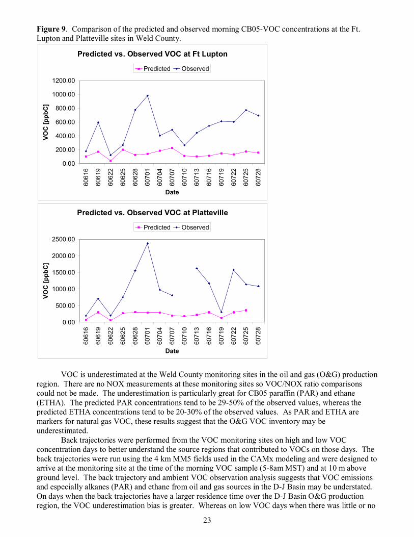
against the modeling results to determine how well the model predicted total VOC concentrations, concentrations of individual VOC species as well as predicting the key VOC/NOx indicator species ratios. The VOC speciation samples were speciated to the CB05 chemical mechanism VOC species used in the modeling. Weld County sites so we can only make model-observed comparisons for total CB05 VOC and Ethane (the VOC comparison is shown in Figure 9). At Fort Lupton, the modeled VOC ranges from 40 to 226 ppbC, whereas the observed values range from 122 to 981 ppbC. Most modeled VOC values at Fort Lupton are between 100-200 ppbC, whereas most observed values are over twice as high ranging from 250 to 700 ppbC. Similar results are seen at Platteville where the modeled VOC ranges from 50 to 200 ppbC, whereas the observed values are much higher ranging from 200 to 2,000 ppbC.
The model is also underpredicting the observed ethane concentrations at the two Weld County sites. At Fort Lupton the observed ethane values range from 24 to 240 ppbC, with average values of around 150 ppbC. Whereas the model ethane predictions range from 6 to 43 ppbC, with average values of approximately 25 ppbC that are over a 100 ppbC lower than observed on average. Even larger ethane underprediction bias is seen at Platteville with observed values of 35 to 600 ppbC and modeled values of 9 to 80 ppbC.
The model systematic underprediction of ethane in Denver and Weld County may suggest that there are missing sources of natural gas in the inventory. Or it may just be due to horizontal and vertical spatial gradients in the observed VOC and ethane concentrations that are not captured by the model grid cell average concentration. VOC species at the two Weld County monitors are dominated by ethane (ETHA) and paraffin (PAR). Table 6 compares the predicted and observed PAR and ETHA concentrations at Fort Lupton and Platteville. The large underprediction of PAR and ETHA at these sites (typically -70% to -80%) indicate that natural gas emissions may be missing in the inventory (Table 6). In addition to underestimating FORM and ALD2, as seen at the two Denver monitoring sites, the aromatic species are also underestimated at the Weld County sites, which suggest that gasoline combustion VOC emissions may be underestimated in the inventory as well.
Table 6. Comparison of predicted and observed morning paraffin (PAR) and ethane (ETHA) concentrations at the Weld County monitoring sites.
Site Date Observed Predicted Difference Difference
(ppbC) (ppbC) (ppbC) (%) PAR
Ft. Lupton June 19 403 119 284 -70% Ft. Lupton July 13 321 67 254 -79% Ft. Lupton July 28 455 105 350 -77% Platteville June 19 484 224 260 -54% Platteville July 28 779 267 512 -66%
ETHA Ft. Lupton June 19 88 18 70 -80% Ft. Lupton July 13 41 9 32 -77% Ft. Lupton July 28 96 13 83 -77% Platteville June 19 97 31 66 -68% Platteville July 28 161 34 127 -79%
23
Figure 9. Comparison of the predicted and observed morning CB05-VOC concentrations at the Ft. Lupton and Platteville sites in Weld County.
VOC is underestimated at the Weld County monitoring sites in the oil and gas (O&G) production
region. There are no NOX measurements at these monitoring sites so VOC/NOX ratio comparisons could not be made. The underestimation is particularly great for CB05 paraffin (PAR) and ethane (ETHA). The predicted PAR concentrations tend to be 29-50% of the observed values, whereas the predicted ETHA concentrations tend to be 20-30% of the observed values. As PAR and ETHA are markers for natural gas VOC, these results suggest that the O&G VOC inventory may be underestimated.
Back trajectories were performed from the VOC monitoring sites on high and low VOC concentration days to better understand the source regions that contributed to VOCs on those days. The back trajectories were run using the 4 km MM5 fields used in the CAMx modeling and were designed to arrive at the monitoring site at the time of the morning VOC sample (5-8am MST) and at 10 m above ground level. The back trajectory and ambient VOC observation analysis suggests that VOC emissions and especially alkanes (PAR) and ethane from oil and gas sources in the D-J Basin may be understated. On days when the back trajectories have a larger residence time over the D-J Basin O&G production region, the VOC underestimation bias is greater. Whereas on low VOC days when there was little or no
Predicted vs. Observed VOC at Ft Lupton
0.00
200.00
400.00
600.00
800.00
1000.00
1200.0060
61
6
60
61
9
60
62
2
60
62
5
60
62
8
60
70
1
60
70
4
60
70
7
60
71
0
60
71
3
60
71
6
60
71
9
60
72
2
60
72
5
60
72
8
Date
VO
C [
pp
bC
]
Predicted Observed
Predicted vs. Observed VOC at Platteville
0.00
500.00
1000.00
1500.00
2000.00
2500.00
60
61
6
60
61
9
60
62
2
60
62
5
60
62
8
60
70
1
60
70
4
60
70
7
60
71
0
60
71
3
60
71
6
60
71
9
60
72
2
60
72
5
60
72
8
Date
VO
C [
pp
bC
]
Predicted Observed

24
residence time over the D-J Basin O&G producing area there is better agreement between the predicted and observed VOC concentrations.
Oil and Gas VOC Sensitivity Simulation
The model performance evaluation and back trajectory analysis using measurements at the Weld
County Fort Lupton and Platteville monitoring sites suggests that oil and gas volatile organic compound (VOC) and ethane emissions may be understated in the photochemical modeling database. To investigate this issue, we performed an oil and gas (O&G) VOC emissions sensitivity test using the CAMx photochemical grid model and the June-July 2006 base case database. For the O&G VOC emissions sensitivity test, VOC emissions from O&G sources were increased by a factor of five. The factor of 5 O&G VOC enhancement factor was entirely arbitrary and should not be interpreted that we believe O&G VOC emissions are underestimated by such a factor. The sensitivity test was designed to see how sensitive ozone formation is to the level of O&G VOC emissions and whether increasing the O&G VOC emissions would improve ozone and VOC model performance. Thus, we wanted to perturb them by a large factor to make sure the change in ozone is above model noise.
CAMx Version 4.51 with the vertical velocity (VV) enhancement was used in the O&G VOC sensitivity test. Previously CAMx VV was used to make a revised 2006 base case and 2020 ozone projections as part of the post Denver 2008 ozone SIP model improvements. The revised CAMx VV 2006 base case simulation (Run22) was compare to the 5 times O&G VOC emissions sensitivity simulation (Run23) to determine the sensitivity of the CAMx VOC and ozone predictions to the level of O&G VOC emissions. Figure 10 compares the daily time series of the predicted and observed morning VOC concentrations at the four monitoring sites for the CAMx base case (Run22) and 5xVOC O&G emissions sensitivity test (Run23). The VOC comparisons in Figure 10 used the sum of the CB05 VOC species, including ethane, to obtain the observed and predicted VOC concentrations. Note that technically these are really total nonmethane organic compound (TNMOC) concentrations because they include ethane, but will call them CB05 VOC concentrations. At the two Weld County monitoring sites, the 5xVOC sensitivity test results in substantial increases in the modeled VOC concentrations so that they match the observed VOC concentrations much better. For example, at the Platteville site, the average observed VOC concentration (970 ppbC) is underestimated in the CAMx Run22 base case simulation (162 ppbC) by a factor of approximately 6. Whereas in the 5xVOC O&G emissions sensitivity test The CAMx Run23 simulation only underestimates the average observed VOC value by -30%.
Figure 10. Observed and predicted TNMOC concentrations for the CAMx base case (Run22) and 5 x VOC O&G emissions sensitivity test.
0200400600800
10001200
6/1
6…
6/1
9…
6/2
2…
6/2
5…
6/2
8…
7/1
/…
7/4
/…
7/7
/…
7/1
0…
7/1
3…
7/1
6…
7/1
9…
7/2
2…
7/2
5…
7/2
8…
VO
C [
pp
bC
]
Date
Predicted vs. Observed VOC at Ft Lupton
Observed Run 22 Run 23

25
Similarly a comparison was conducted between the base case (Run 22) and 5x sensitivity run
(Run 23) for predicted ozone model performance at the three monitoring sites for four 3-day episode periods during the June-July 2006 modeling period. The three monitoring sites are the Rocky Flats North (RFNO) monitor, which over the last decade has had the highest ozone Design Value in the DMA/NFR region, the Fort Collins West (FTCW) monitor which also observed high ozone but is improving, and Weld County Tower (WCTO) monitoring site that is near Greeley north of Platteville and within the D-J Basin O&G production region. During June 17-19, 2006 episode, the 5xVOC O&G emissions sensitivity test has no effect on the predicted ozone concentrations on the first two days (June 17-18). On June 19th there is a slight (~2 ppb) increase in the hourly ozone between 6am and noon at the RFNO and FTCW monitoring sites, but little to no effect the remainder of the time. During the June 26-28, 2006 episode the CAMx hourly ozone peak at RFNO on June 26 increases from 66.0 to 69.7 ppb due to the 5xVOC sensitivity test with slightly higher ozone also seen at RFNO on June 27 but no change on June 28. Very small ozone increases are also seen at FTCW and WCTO. There is essentially no change in the predicted ozone at RFNO and FTCW due to the 5xVOC sensitivity test during the July 13-15, 2006 episode. At the WCTO monitor, small increases in ozone are seen due to the 5xVOC sensitivity test. This includes the model trying to replicate a sharp rise in the observed morning ozone on July 15th where the ozone increases 6 ppb at 10am from 69 to 75 ppb due to the 5xVOC sensitivity simulation. The July 27-29, 2006 episode has slow wind speeds, consequently the largest changes in ozone occur at the WCTO monitoring site. The hourly ozone peaks at WCTO are increased from 81 to 85 ppb (+4 ppb) and from 82 to 87 ppb (+5 ppb) on, respectively, July 28 and 29 due to the 5xVOC O&G emissions sensitivity test better matching the observed ozone peaks on these two days.
The five times oil and gas VOC emissions sensitivity test produced slightly improved ozone model performance on some days at some of the monitoring sites. However, it resulted in significant improvement in VOC model performance at the two Weld County monitoring sites. These results suggest that VOC emissions may be understated in the D-J Basin, however the results are inconclusive as the VOC underestimation could also be due to spatially variability in the VOC concentrations that is not captured by the model grid cell average predictions.
The single largest source of VOC emissions from O&G sources in the D-J Basin are flash emissions from condensate tanks. Large condensate tanks are required to control these emissions, but smaller tanks are not. There is a lot of spatial variability in VOC emissions and consequently VOC concentrations across the D-J Basin. The model fails to capture all of this spatial variability due in part to use of the 4 km grid resolution. The model is also using average emissions rates that fail to capture the real-world temporal variability in emissions, including O&G production emissions. Some of the highest observed VOC concentrations (e.g., July 1, 2006 at Platteville) are likely due in part to temporal variations in the real-world emissions not captured in the emissions modeling. If the monitors are located close to some of these VOC sources then that could be a source of a model VOC underestimation bias, when in reality it is just an artifact of the averaging that is done in the model. The ozone increases due to the 5xVOC O&G emissions sensitivity test are small in the context of an ozone model performance evaluation that compares predicted and observed ozone concentrations. However, in
0
500
1000
1500
2000
2500
6/1
6
6/1
9
6/2
2
6/2
5
6/2
8
7/1
7/4
7/7
7/1
0
7/1
3
7/1
6
7/1
9
7/2
2
7/2
5
7/2
8
VO
C [
pp
bC
]
Date
Predicted vs. Observed VOC at Platteville
Observed Run 22 Run 23

26
the context of emissions control strategy evaluation in attainment demonstration modeling, a few ppb change in ozone is quite significant.
CMB and PMF Receptor Modeling
In this section we discuss the application of receptor models to the measured VOC species
concentrations in the Denver area during the June-July 2006 modeling episode for the purpose of trying to resolve differences between the measured ambient VOC concentrations and the VOC emissions inventory used in the photochemical grid modeling.
Receptor models, also called observation based models (OBM), use measured concentrations and estimate what source types contributed to them. In this study we used detailed speciated VOC measurements of numerous individual VOC species and receptor models to estimate source contributions to the VOC measurements. The two receptor models used were the Chemical Mass Balance (CMB) and the Positive Matrix Factorization (PMF). In the CMB receptor model, speciated VOC source profiles (source VOC finger prints) are provided and the CMB tries to fit those source profiles to the VOC measurements and estimate VOC source contributions to the measured VOC concentrations. The PMF receptor model decomposes the VOC measurements into “factors” that have different key VOC species and then the user examines the factors’ VOC speciation profiles to infer what types of sources emit those types of VOC profiles (i.e., what source category do the factors represent). In CMB, accurate and representative source profiles specific to the region of interest are needed as input in order to obtain reliable VOC source apportionment. CMB has a disadvantage in that potentially a large amount of the VOC measurement may be unidentifiable if it does not fit any of the provided source profiles. PMF has an advantage in that you do not have to a prior define the source profiles and it determines the factors based on the speciated VOC measurements. This can be an important attribute if there is a strong source signature for a source type that you don’t have source profiles for when CMB is used. However, PMF has a disadvantage in that it requires many more speciated VOC measurements than CMB to develop its factors and that the PMF factors may be nonsensical or represent multiple source types so are difficult to interpret.
In this study we first applied the CMB model to obtain preliminary CMB VOC source apportionment. We then made a preliminary application of PMF using just the VOC species in the CMB VOC source profiles and compared it with the CMB source apportionment. The PMF application helped identify additional VOC source profiles that were then used in a revised CMB application. We also performed a revised PMF application using all of the measured VOC species in the measurement, rather than just the VOC species in the CMB VOC speciation profiles used in the preliminary PMF application. Detailed technical formulations of both the CMB and PMF models can be found in the technical report for the study16.
The preliminary CMB modeling was applied to the morning (5-8am) VOC samples at the two Weld County monitoring sites. The preliminary CMB receptor modeling used the following VOC source profiles:
Compressed Natural Gas (CNG) Geogenic Natural Gas (GNG) Liquid Petroleum Gas (LPG) Gas Evaporative (Gas Evap) Vehicle Exhaust (Gasoline Combustion) Biogenic
The leftover VOC mass classified as “unidentified” represents the unknown species from the
measured VOC that are not represented in the input VOC source profiles. The CNG, GNG, LPG and Gas Evap profiles correspond to oil and gas sources. This would include oil and gas exploration and productions, as well as oil and gas processing and use. The Vehicle Exhaust profile corresponds to gasoline combustion within on-road mobile sources, as well as non-road gasoline engines and stationary

27
source gasoline combustion. The biogenic profile is keyed in on isoprene that is primarily emitted by deciduous trees.
The CMB model was applied to the morning speciated VOC measurements at the two Weld County sites using samples from the June-July 2006 period and the six VOC source profiles discussed above. There were 14-16 morning samples at each monitoring site. Figure 11 displays the source category contributions estimated by CMB averaged across the 14-16 sample days at the Fort Lupton and Platteville monitoring sites. As expected, the VOC contributions attributable to vehicle exhaust is relatively small at the two Weld County sites (6% and 2%), and the contribution of source categories associated with oil and gas sources is relatively high at the two Weld County sites (94% and 98%). The biogenic contribution was extremely low for all sites.
Figure 11. Average source contribution to measured VOC concentrations at four monitoring sites estimated using the preliminary CMB receptor modeling.
The CMB-estimated CNG source contributions appear to be highest at Fort Lupton, although the
unidentified fraction and Gas Evap contributions can also be high on some days. The signal of the four source categories associated with oil and gas is greatest at the Platteville monitoring site, which is consistent with its location in the center of the D-J Basin oil and gas producing area. On June 28, 2006, the CMB estimates that 1,600 ppbC of VOC is contributed by CNG, GNG, LPG and Gas Evap source categories.
The large fraction of measured VOC not speciated was a cause for concern indicating that there are additional VOCs which cannot be attributed to sources by the CMB receptor model. Another area of concern was the low biogenic VOC contribution estimated by the preliminary CMB modeling. To help identify potential additional source profiles that could be used, the PMF receptor model was applied. As noted previously, the PMF does not use source profiles as input but instead analyzes the VOC speciation data to obtain VOC speciation factors that may be attributable to a particular source category.
The PMF receptor model was used initially to try and better understand and potentially refine the preliminary CMB VOC source apportionment modeling results. The PMF was configured initially to use just the VOC species used in the preliminary CMB application. That is, the VOC species in the CNG, GNG, LPG Gas Evap, Vehicle Exhaust and Biogenic VOC speciation profiles were provided as input to PMF for the ~60 VOC measurements. The PMF was exercised using 4 and 5 factors. The 4 factor PMF application produced more recognizable source factors so is reported here. We examined the four factors produced by the PMF receptor modeling and found three of them produced a good match with the CMB VOC speciation profiles.
Veh Exh6%
CNG35%
GNG13%
LPG14%
Biogenic0%
Gas Evap.32%
Ft. LuptonVeh Exh
2%
CNG37%
GNG11%LPG
16%
Biogenic0%
Gas Evap.34%
Platteville

28
Figure 12 compares the four PMF factor VOC speciation profiles with VOC source profiles from the CMB collection. The first PMF factor is compared against the composite VOC source profile for CNG, GNG, LPG and Gas Evap, which is representative of VOC emissions from oil and gas production, processing and use. Both PMF and the composite VOC profile agree that N-Propane (N_PROP) is the largest component followed by Ethane (ETHANE) and then N-Butane (N_BUTA). There are also contributions of Iso-Butane (I_BUTA) and Iso-Pentane (IPENTA) in the first factor.
The second PMF factor compares favorably with the cold start emissions VOC speciation profile (Figure 12, second panel). Although the match is not as good as seen with the PMF factor 1 oil and gas VOC profile, there are numerous key species associated with cold start VOC emissions that are present in the second PMF factor (e.g., aromatics species of Benzene, Toluene and Xylene or BTX). PMF factor 2 does overstate the contributions of Ethane and Iso-Pentane to the vehicle cold start VOC profile. Note that the vehicle cold start VOC emissions profile was not used in the preliminary CMB modeling because of concern it could be co-linear with the vehicle running exhaust VOC profile.
The third PMF factor VOC species contribution has a fairly good match with the vehicle running exhaust VOC profile (Figure 12, third panel). Ethane and N-Butane are matched well, although the PMF third factor understates N-Propane.
The final PMF factor does not appear to match any of the profiles very well. In Figure 12 (bottom) the fourth PMF factor is compared to a composite solvent and biogenic VOC speciation profile, as these are two of the largest remaining source categories not accounted for in the previous three PMF factors. However, PMF factor four has a poor match with biogenic and solvent VOC speciation profiles.
Figure 12. VOC source profiles for the four PMF factors compared against VOC speciation profiles that can be used as input into CMB.
0%
5%
10%
15%
20%
25%
30%
35%
40%
BZ1
23
M
BZ1
24
M
BZ1
35
M
PEN
TE1
PA
224
M
BU
22
DM
PA
234
M
BU
23
DM
PEN
23
M
PEN
24
M
HEP
2ME
HEX
A2
M
PEN
A2
M
HEP
3ME
HEX
A3
M
PEN
A3
M
AC
ETYL
BEN
ZE
C2
BU
TE
C2
PEN
E
CYH
EXA
CP
ENTA
ETH
AN
E
ETB
Z
I_B
UTA
LBU
T1
E
IPEN
TA
I_P
RE
N
DET
BZ1
MEC
YH
X
MC
YPN
A
M_E
TOL
MP
_XYL
N_B
UTA
N_D
EC
N_H
EPT
N_H
EX
N_N
ON
N_O
CT
N_P
ENT
N_P
RB
Z
N_U
ND
E
O_E
TOL
O_X
YL
P_E
TOL
N_P
RO
P
STYR
TOLU
E
T2B
UTE
T2PE
NE
Oil & Gas Emissions Profiles (CMB = CNG + GNG + LPG + GEVAP)
PMF
CMB
0%
2%
4%
6%
8%
10%
12%
14%
16%
18%
BZ1
23
M
BZ1
24
M
BZ1
35
M
PEN
TE1
PA
22
4M
BU
22D
M
PA
23
4M
BU
23D
M
PEN
23
M
PEN
24
M
HEP
2M
E
HEX
A2
M
PEN
A2
M
HEP
3M
E
HEX
A3
M
PEN
A3
M
AC
ETY
L
BEN
ZE
C2
BU
TE
C2
PEN
E
CYH
EXA
CP
ENTA
ETH
AN
E
ETB
Z
I_B
UTA
LBU
T1E
IPEN
TA
I_P
REN
DET
BZ1
MEC
YHX
MC
YPN
A
M_E
TOL
MP
_XYL
N_B
UTA
N_D
EC
N_H
EPT
N_H
EX
N_N
ON
N_O
CT
N_P
ENT
N_P
RB
Z
N_U
ND
E
O_E
TO
L
O_X
YL
P_E
TOL
N_P
RO
P
STYR
TOLU
E
T2B
UTE
T2PE
NE
Vehicle Cold Start Emissions Profiles
PMF
CMB
0%
5%
10%
15%
20%
25%
30%
35%
40%
BZ1
23
M
BZ1
24
M
BZ1
35
M
PEN
TE1
PA
22
4M
BU
22
DM
PA
23
4M
BU
23
DM
PEN
23
M
PEN
24
M
HEP
2M
E
HE
XA
2M
PEN
A2
M
HEP
3M
E
HE
XA
3M
PEN
A3
M
AC
ETY
L
BEN
ZE
C2
BU
TE
C2
PEN
E
CYH
EXA
CP
ENTA
ETH
AN
E
ETB
Z
I_B
UTA
LBU
T1E
IPEN
TA
I_P
REN
DET
BZ1
MEC
YHX
MC
YPN
A
M_E
TO
L
MP
_XYL
N_B
UTA
N_D
EC
N_H
EPT
N_H
EX
N_N
ON
N_O
CT
N_P
ENT
N_P
RB
Z
N_U
ND
E
O_E
TOL
O_
XYL
P_E
TOL
N_P
RO
P
STYR
TOLU
E
T2B
UTE
T2P
ENE
Vehicle Running Emissions Profiles
PMF
CMB

29
Based on the PMF modeling, we identified two additional VOC profiles (vehicle cold starts and
solvent) for the revised CMB receptor modeling. The revised CMB modeling used the following VOC source profiles: CNG; GNG; LPG; Gas Evap; Gasoline Combustion; Bio; Veh Cold Start; and Solvent. The CMB-estimated VOC source contributions for CNG, GNG, LPG and Gas Evap were combined together to represent the oil and gas (O&G) source sector. Note that in the preliminary CMB application we were careful not to provide too many VOC source profiles as that can degrade the CMB source apportionment, especially when the VOC source profiles were co-linear. For example, specifying VOC source profiles for vehicle exhaust and vehicle cold starts could cause problems in the CMB modeling due to their co-linearity. However, the PMF modeling demonstrated that these two signals are sufficiently unique that this should not be a problem.
Figure 13 compares the daily VOC contributions estimated by the preliminary PMF and revised CMB receptor modeling using the source categories associated with the four PMF factors. With four sites and 14-16 days for each site this results in approximately 60 comparisons. Note that although the PMF factors were used to help identify additional VOC source profiles to use in the revised CMB modeling, the PMF and CMB VOC source apportionment receptor modeling are completely separate and independent calculations.
The agreement between the PMF factor 1 and CMB O&G VOC source apportionment is quite good (Figure 13, top panel). The day-to-day VOC contributions associated with vehicle cold start emissions estimated by PMF and CMB is not as good as seen for O&G sources, but they do tend to follow the trends in each other well at Fort Lupton (FLCO) (Figure 13, second panel). Agreement between PMF and CMB cold start VOC contributions is fairly good at Fort Lupton, but not as good at Platteville where CMB estimates higher contributions than PMF.
A comparison of the VOC contribution due to vehicle running exhaust emissions is given in the third panel in Figure 13 and shows good agreement in the day-to-day variations at Fort Lupton, with CMB estimating a much higher contribution than PMF. There is poor agreement in both the trends and magnitude in the VOC due to vehicle running exhaust emissions at Platteville with PMF estimating much higher contributions compared to CMB. Finally, the bottom panel in Figure 13 compares the PMF fourth factor VOC contributions with the CMB VOC contributions from solvent and biogenic sources. Not surprisingly given the poor agreement between the PMF and CMB VOC speciation profiles for this factor (see Figure 12, bottom), the VOC source contributions also has poor agreement.
Figure 13. Comparison of PMF and revised CMB VOC source contributions (ppbC) for the four PMF factors and their counterparts in the revised CMB modeling.
0%
10%
20%
30%
40%
50%
60%
BZ1
23
M
BZ1
24
M
BZ1
35
M
PEN
TE1
PA2
24
M
BU
22D
M
PA
234
M
BU
23D
M
PEN
23
M
PEN
24
M
HEP
2M
E
HEX
A2
M
PEN
A2
M
HEP
3M
E
HEX
A3
M
PEN
A3
M
AC
ETY
L
BEN
ZE
C2
BU
TE
C2
PEN
E
CYH
EXA
CP
ENTA
ETH
AN
E
ETB
Z
I_B
UTA
LBU
T1
E
IPE
NTA
I_P
REN
DE
TBZ1
MEC
YHX
MC
YPN
A
M_E
TOL
MP
_XYL
N_B
UT
A
N_D
EC
N_H
EPT
N_H
EX
N_N
ON
N_O
CT
N_P
ENT
N_P
RB
Z
N_
UN
DE
O_E
TO
L
O_X
YL
P_E
TOL
N_P
RO
P
STYR
TOLU
E
T2B
UTE
T2P
ENE
Remaining Sources Profile Comparison (CMB = Sovent + Biogenic)
PMF
CMB
0
500
1000
1500
2000
2500
3000
DE
CO
06
/16
/20
06
DE
CO
06
/19
/20
06
DE
CO
06
/22
/20
06
DE
CO
06
/25
/20
06
DE
CO
06
/28
/20
06
DE
CO
07
/01
/20
06
DE
CO
07
/04
/20
06
DE
CO
07
/07
/20
06
DE
CO
07
/10
/20
06
DE
CO
07
/13
/20
06
DE
CO
07
/16
/20
06
DE
CO
07
/19
/20
06
DE
CO
07
/22
/20
06
DE
CO
07
/25
/20
06
DE
CO
07
/28
/20
06
DE
CO
07
/31
/20
06
WE
CO
06
/16
/20
06
WE
CO
06
/19
/20
06
WE
CO
06
/22
/20
06
WE
CO
06
/25
/20
06
WE
CO
06
/28
/20
06
WE
CO
07
/01
/20
06
WE
CO
07
/04
/20
06
WE
CO
07
/07
/20
06
WE
CO
07
/10
/20
06
WE
CO
07
/13
/20
06
WE
CO
07
/16
/20
06
WE
CO
07
/19
/20
06
WE
CO
07
/22
/20
06
WE
CO
07
/25
/20
06
WE
CO
07
/31
/20
06
FLC
O 0
6/1
6/2
00
6
FLC
O 0
6/1
9/2
00
6
FLC
O 0
6/2
2/2
00
6
FLC
O 0
6/2
5/2
00
6
FLC
O 0
6/2
8/2
00
6
FLC
O 0
7/0
1/2
00
6
FLC
O 0
7/0
4/2
00
6
FLC
O 0
7/0
7/2
00
6
FLC
O 0
7/1
0/2
00
6
FLC
O 0
7/1
3/2
00
6
FLC
O 0
7/1
6/2
00
6
FLC
O 0
7/1
9/2
00
6
FLC
O 0
7/2
2/2
00
6
FLC
O 0
7/2
5/2
00
6
FLC
O 0
7/2
8/2
00
6
FLC
O 0
7/3
1/2
00
6
PLC
O 0
6/1
6/2
006
PLC
O 0
6/1
9/2
006
PLC
O 0
6/2
2/2
006
PLC
O 0
6/2
5/2
006
PLC
O 0
6/2
8/2
006
PLC
O 0
7/0
1/2
006
PLC
O 0
7/0
7/2
006
PLC
O 0
7/1
0/2
006
PLC
O 0
7/1
6/2
006
PLC
O 0
7/1
9/2
006
PLC
O 0
7/2
2/2
006
PLC
O 0
7/2
5/2
006
PLC
O 0
7/2
8/2
006
PLC
O 0
7/3
1/2
006
Co
nce
ntr
atio
n (
pp
bC
)
Oil & Gas Emissions (CMB = CNG + GNG + LPG + GEVAP) (ppbC)
PMF
CMB

30
Figure 14 displays the revised CMB VOC source apportionment modeling results averaged
across all monitoring days at the two Weld County monitoring sites that can be compared with Figure 11 for the preliminary CMB modeling. The revised CMB modeling estimates slightly lower VOC at Fort Lupton due to oil and gas sources (89%) compared to the preliminary CMB modeling (94%), this appears to be due in part to the new solvent category as the motor vehicle (7%) remain approximately the same. At Platteville, the contribution of vehicle running exhaust emissions remained the same in the preliminary and revised CMB modeling (1%), but the vehicle cold start emissions added another 2% contribution to motor vehicles. The new cold start (2%) and solvent (3%) source categories appear to have reduced the O&G contributions from 98% to 94% in the revised CMB modeling.
The conclusions in the revised CMB modeling remain the same as the preliminary CMB modeling with the two Weld County monitoring sites seeing a large contribution from O&G sources. But the comparison of the PMF and CMB VOC source apportionment modeling results provide some confidence in the CMB and PMF VOC contributions of O&G and motor vehicle source sectors to the measured VOC concentrations.
0
20
40
60
80
100
120
DE
CO
06
/16
/200
6
DE
CO
06
/19
/200
6
DE
CO
06
/22
/200
6
DE
CO
06
/25
/200
6
DE
CO
06
/28
/200
6
DE
CO
07
/01
/200
6
DE
CO
07
/04
/200
6
DEC
O 0
7/0
7/2
006
DE
CO
07
/10
/200
6
DE
CO
07
/13
/200
6
DE
CO
07
/16
/200
6
DEC
O 0
7/1
9/2
006
DE
CO
07
/22
/200
6
DE
CO
07
/25
/200
6
DE
CO
07
/28
/200
6
DE
CO
07
/31
/200
6
WE
CO
06
/16
/20
06
WE
CO
06
/19
/20
06
WE
CO
06
/22
/20
06
WE
CO
06
/25
/20
06
WE
CO
06
/28
/20
06
WE
CO
07
/01
/20
06
WE
CO
07
/04
/20
06
WE
CO
07
/07
/20
06
WE
CO
07
/10
/20
06
WE
CO
07
/13
/20
06
WE
CO
07
/16
/20
06
WE
CO
07
/19
/20
06
WE
CO
07
/22
/20
06
WE
CO
07
/25
/20
06
WE
CO
07
/31
/20
06
FLC
O 0
6/1
6/2
00
6
FLC
O 0
6/1
9/2
00
6
FLC
O 0
6/2
2/2
00
6
FLC
O 0
6/2
5/2
00
6
FLC
O 0
6/2
8/2
00
6
FLC
O 0
7/0
1/2
00
6
FLC
O 0
7/0
4/2
00
6
FLC
O 0
7/0
7/2
00
6
FLC
O 0
7/1
0/2
00
6
FLC
O 0
7/1
3/2
00
6
FLC
O 0
7/1
6/2
00
6
FLC
O 0
7/1
9/2
00
6
FLC
O 0
7/2
2/2
00
6
FLC
O 0
7/2
5/2
00
6
FLC
O 0
7/2
8/2
00
6
FLC
O 0
7/3
1/2
00
6
PLC
O 0
6/1
6/2
00
6
PLC
O 0
6/1
9/2
00
6
PLC
O 0
6/2
2/2
00
6
PLC
O 0
6/2
5/2
00
6
PLC
O 0
6/2
8/2
00
6
PLC
O 0
7/0
1/2
00
6
PLC
O 0
7/0
7/2
00
6
PLC
O 0
7/1
0/2
00
6
PLC
O 0
7/1
6/2
00
6
PLC
O 0
7/1
9/2
00
6
PLC
O 0
7/2
2/2
00
6
PLC
O 0
7/2
5/2
00
6
PLC
O 0
7/2
8/2
00
6
PLC
O 0
7/3
1/2
00
6
Co
nce
ntr
atio
n (
pp
bC
)
Vehicle Cold Start Emissions (ppbC)
PMF
CMB
020406080
100120140160180
DE
CO
06
/16
/200
6
DE
CO
06
/19
/200
6
DE
CO
06
/22
/200
6
DE
CO
06
/25
/200
6
DE
CO
06
/28
/200
6
DE
CO
07
/01
/200
6
DE
CO
07
/04
/200
6
DE
CO
07
/07
/200
6
DE
CO
07
/10
/200
6
DE
CO
07
/13
/200
6
DE
CO
07
/16
/200
6
DE
CO
07
/19
/200
6
DE
CO
07
/22
/200
6
DE
CO
07
/25
/200
6
DE
CO
07
/28
/200
6
DE
CO
07
/31
/200
6
WE
CO
06
/16
/20
06
WE
CO
06
/19
/20
06
WE
CO
06
/22
/20
06
WE
CO
06
/25
/20
06
WE
CO
06
/28
/20
06
WE
CO
07
/01
/20
06
WE
CO
07
/04
/20
06
WE
CO
07
/07
/20
06
WE
CO
07
/10
/20
06
WE
CO
07
/13
/20
06
WE
CO
07
/16
/20
06
WE
CO
07
/19
/20
06
WE
CO
07
/22
/20
06
WE
CO
07
/25
/20
06
WE
CO
07
/31
/20
06
FLC
O 0
6/1
6/2
00
6
FLC
O 0
6/1
9/2
00
6
FLC
O 0
6/2
2/2
00
6
FLC
O 0
6/2
5/2
00
6
FLC
O 0
6/2
8/2
00
6
FLC
O 0
7/0
1/2
00
6
FLC
O 0
7/0
4/2
00
6
FLC
O 0
7/0
7/2
00
6
FLC
O 0
7/1
0/2
00
6
FLC
O 0
7/1
3/2
00
6
FLC
O 0
7/1
6/2
00
6
FLC
O 0
7/1
9/2
00
6
FLC
O 0
7/2
2/2
00
6
FLC
O 0
7/2
5/2
00
6
FLC
O 0
7/2
8/2
00
6
FLC
O 0
7/3
1/2
00
6
PLC
O 0
6/1
6/2
006
PLC
O 0
6/1
9/2
006
PLC
O 0
6/2
2/2
006
PLC
O 0
6/2
5/2
006
PLC
O 0
6/2
8/2
006
PLC
O 0
7/0
1/2
006
PLC
O 0
7/0
7/2
006
PLC
O 0
7/1
0/2
006
PLC
O 0
7/1
6/2
006
PLC
O 0
7/1
9/2
006
PLC
O 0
7/2
2/2
006
PLC
O 0
7/2
5/2
006
PLC
O 0
7/2
8/2
006
PLC
O 0
7/3
1/2
006
Co
nce
ntr
atio
n (p
pb
C)
Vehicle Running Emissions (ppbC)
PMF
CMB
-100
1020304050607080
DE
CO
06
/16
/20
06
DE
CO
06
/19
/20
06
DE
CO
06
/22
/20
06
DE
CO
06
/25
/20
06
DE
CO
06
/28
/20
06
DE
CO
07
/01
/20
06
DE
CO
07
/04
/20
06
DE
CO
07
/07
/20
06
DE
CO
07
/10
/20
06
DE
CO
07
/13
/20
06
DE
CO
07
/16
/20
06
DE
CO
07
/19
/20
06
DE
CO
07
/22
/20
06
DE
CO
07
/25
/20
06
DE
CO
07
/28
/20
06
DE
CO
07
/31
/20
06
WEC
O 0
6/1
6/2
00
6
WEC
O 0
6/1
9/2
00
6
WEC
O 0
6/2
2/2
00
6
WEC
O 0
6/2
5/2
00
6
WEC
O 0
6/2
8/2
00
6
WEC
O 0
7/0
1/2
00
6
WEC
O 0
7/0
4/2
00
6
WEC
O 0
7/0
7/2
00
6
WEC
O 0
7/1
0/2
00
6
WEC
O 0
7/1
3/2
00
6
WEC
O 0
7/1
6/2
00
6
WEC
O 0
7/1
9/2
00
6
WEC
O 0
7/2
2/2
00
6
WEC
O 0
7/2
5/2
00
6
WEC
O 0
7/3
1/2
00
6
FLC
O 0
6/1
6/2
00
6
FLC
O 0
6/1
9/2
00
6
FLC
O 0
6/2
2/2
00
6
FLC
O 0
6/2
5/2
00
6
FLC
O 0
6/2
8/2
00
6
FLC
O 0
7/0
1/2
00
6
FLC
O 0
7/0
4/2
00
6
FLC
O 0
7/0
7/2
00
6
FLC
O 0
7/1
0/2
00
6
FLC
O 0
7/1
3/2
00
6
FLC
O 0
7/1
6/2
00
6
FLC
O 0
7/1
9/2
00
6
FLC
O 0
7/2
2/2
00
6
FLC
O 0
7/2
5/2
00
6
FLC
O 0
7/2
8/2
00
6
FLC
O 0
7/3
1/2
00
6
PLC
O 0
6/1
6/2
006
PLC
O 0
6/1
9/2
006
PLC
O 0
6/2
2/2
006
PLC
O 0
6/2
5/2
006
PLC
O 0
6/2
8/2
006
PLC
O 0
7/0
1/2
006
PLC
O 0
7/0
7/2
006
PLC
O 0
7/1
0/2
006
PLC
O 0
7/1
6/2
006
PLC
O 0
7/1
9/2
006
PLC
O 0
7/2
2/2
006
PLC
O 0
7/2
5/2
006
PLC
O 0
7/2
8/2
006
PLC
O 0
7/3
1/2
006
Co
nce
ntr
atio
n (p
pb
C)
Remaining Source Comparison (CMB = Solvent + Biogenic) (ppbC)
PMF
CMB

31
Figure 14. Average source contribution to measured VOC concentrations at monitoring sites estimated using the revised CMB receptor modeling.
Emission Based VOC Source Apportionment Modeling The CMB and PMF VOC source apportionment modeling presented two realizations of the
“sources” that contributed to the morning VOC measurements collected during the June-July 2006 period. In the past, such receptor modeling based VOC source apportionment results have been compared against the emissions inventory to try an reconcile the differences between the VOC emissions inventory and the receptor modeling VOC source apportionment based on the VOC measurements. However, it is unclear how big an area around the monitoring sites should be included in the VOC emissions inventory comparison. Upwind sector averaging can be used to refine the selected VOC inventory area for comparison with the receptor modeling VOC contributions, but there are still issues with how far upwind to look and what to do when wind varies. To get around this issue we performed VOC source apportionment modeling using the CAMx probing tools. The Ozone Source Apportionment Technology (OSAT) was used to track VOC emissions from major source categories that were then extracted at the monitoring sites for the 5-8am MST period and compared with the CMB and PMF receptor modeling VOC source apportionment results. In this application we analyzed the VOC tracers to determine major source category contributions to VOC concentrations at the time and locations that the VOC measurements were made. The CAMx/OSAT VOC source apportionment modeling tracked ozone, VOC and NOX contributions during the June-July 2006 episode for the following source categories: Biogenic, On-Road Mobile, Non-Road Mobile, Oil and Gas Production, Area, and Point.
Figure 15 displays the relative contributions of VOC source contributions at the two Weld County monitoring sites averaged across the VOC morning sampling times estimated by the CAMx/OSAT emissions-based source apportionment modeling and the revised CMB and PMF receptor modeling. All three source apportionment techniques estimate that O&G is the largest contributor to VOC concentrations at Fort Lupton and especially Platteville. CAMx/OSAT estimates higher contributions of mobile, area/point and biogenic than the two receptor models. It is suspected that sources that CMB/PMF attributes to oil and gas are within the area/point and mobile source categories in the CAMx/OSAT modeling.
Exhaust4%
Cold Starts
3%
O&G89%
Biogenic0%
Solvents4%
Ft. LuptonExhaust
1%Cold
Starts2%
O&G94%
Biogenic0%
Solvents3%
Platteville

32
Figure 15. Comparison of the relative contributions of VOC source categories to the average VOC concentrations at the Fort Lupton and Platteville Weld County monitoring sites.
The comparison of the emissions based deterministic CAMx/OSAT VOC source apportionment
modeling results with the observation-based CMB and PMF receptor modeling VOC source apportionment modeling results is inconclusive because of the following:
The CAMx/OSAT, CMB and PMF VOC source categories do not represent the same sources so this is not an “apple-apple” comparison. The CAMx biogenic, mobile, oil and gas and area/point are well defined from the pre-merged emission files. But the PMF and CMB oil and gas category likely contains some sources in the CAMx/OSAT mobile and area/point categories.
The PMF VOC source apportionment is not precise instead being mathematical factors that are interpreted as specific source categories. In reality they are mixture of sources (e.g., ethane in the biogenic source category).
It is difficult to determine whether the CAMx VOC underestimation bias is due to insufficient VOC emissions or just differences between the surface-based point measurement versus the grid cell volume average model prediction.
Despite these limitations, there is evidence that VOC emissions in the oil and gas production area
of Weld County may be under represented in the VOC emissions inventories. The largest source of VOC emission in the oil and gas production is flash emissions from the condensate tanks. Regulation 7 (Reg 7) requires large condensate tanks to have 95% control, which is what was provided in the Reg 7 reports used to develop the oil and gas emissions in the D-J Basin under WRAP Phase III. Note that a

33
small reduction in control efficiency would result in a large increase in VOC emissions from these sources.
FUTURE WORK
The work presented here shows that improvements have been made and implemented in the WRAP methodologies for basin level inventories. Despite this, a recent study of the reconciliation between measured VOC concentrations and model predicted concentrations suggests that these inventories are still underpredicting VOCs. Recent work by NOAA in taking aircraft-based flux measurements of methane in oil and gas basins also confirms the underestimation of emissions from oil and gas17. In response to this, the NETL has funded a research group comprised of NOAA, NREL, CSU and the Colorado School of Mines to study the reconciliation of top-down measurements and bottom-up inventories of methane from oil and gas.
The bottom-up inventory portion of the study will consist of further improvements to the methodologies initially used in the WRAP Phase III basin inventories. Some of these improvements include:
Temporal resolution – the inventory will focus on a time period concurrent with the top-down field measurements such that a highly temporally resolved inventory will be developed for direct comparison with the top-down measurements (order of several weeks).
Episodic emission inventory – the study will develop a survey for operators that is focused specifically on episodic emissions events, such as maintenance and upset conditions, well liquids unloading, well completions, and vessel and compressor blowdowns. The data gathered from the surveys will provide an enhanced set of activity data to estimate emissions from these non-routine events which have often been either missing from inventories or captured at a very coarse temporal resolution.
Focus on midstream and transmission sectors – building on the findings of the previous WRAP inventories, significant efforts will be made to identify and include midstream gathering and processing companies and transmission and distribution companies in the survey effort. Past work has shown that midstream gathering and processing facilities are often undercounted in oil and gas inventories, including gathering pipelines, compressor stations, liquid knockout, tank batteries and other similar sources. Both routine and episodic activity surveys will be developed for these sectors.
Use of latest emission factors – leveraging the extensive observation-based emissions factors developed as part of the EDF study of oil and gas emissions, the emission factors will include the latest data on pneumatic devices, fugitive components and other emission source factors reported as part of the EDF study.
Uncertainty analysis – variability in activity data and the uncertainty and probability distributions of the emissions factors from the EDF study will allow for a Monte Carlo-type uncertainty analysis to be performed on the resulting inventory. This will be the first basin-level oil and gas inventory to explicitly attempt to evaluate uncertainty for better comparison to the top-down measurements.
The study began in 2014 and is expected to continue through 2016. Results will be published in
peer-reviewed journals once available, and will include presentations and outreach/educational efforts to broadly publicize the results of the work once available. REFERENCES
1. Russell, J.; Pollack, A.K., “Oil and Gas Emission Inventories for the Western States”; Prepared for Western Governors’ Association by ENVIRON International Corporation, Novato, CA 2005.
34
2. Bar-Ilan, A.; Friesen, R.; Pollack, A.; Hoats, A., “WRAP Area Source Emissions Inventory Protections and Control Strategy Evaluation Phase II”; Prepared for Western Governors’ Association by ENVIRON International Corporation, Novato, CA 2007.
3. WRAP Phase III. http://www.wrapair2.org/PhaseIII.aspx (accessed July 2012). 4. Bar-Ilan, A.; Grant, J.; Parikh, R.; Morris, R.; Henderer, D., “Oil and Gas Mobile Sources Pilot
Study”; Prepared for US EPA by ENVIRON International Corporation, Novato, CA 2011. 5. WRAP West-wide Jumpstart Air Quality Modeling Study (WestJumpAQMS); Prepared for
Western Governors’ Association by ENVIRON International Corporation, Novato, CA 2013. http://www.wrapair2.org/WestJumpAQMS.aspx (accessed April 2015).
6. WRAP Intermountain States Data Warehouse. http://views.cira.colostate.edu/tsdw/ (accessed April 2015)
7. Morris, R.; Wang, B.; Tai, E.; McNally, D.; Loomis, C.; Stella G.; Tesche, T.W., “Modeling Protocol for the Denver 8-Hour Ozone Attainment Demonstration Modeling”; Prepared for Denver Regional Air Quality Council by ENVIRON International Corporation, Novato, CA 2007. http://www.colorado.gov/airquality/documents/deno308/Draft_Final_Protocol_Denver_8-Hour_Ozone_Nov28_2007.pdf
8. EPA. “2011 National Modeling Platform; 2011 NEIv2-based Platform (2011 v6.2)”; U.S. Environmental Protection Agency, Research Triangle Park, NC 2015. http://www.epa.gov/ttn/chief/emch/index.html#2011 (accessed April 2015).
9. Grant, J.; Parikh, R.; Bar-Ilan, A.; Morris, R., “Development of Baseline 2011 and Future Year 2015 Emissions from Oil and Gas Activity in the Williston Basin”; Prepared for Susan Bassett, BLM and Tom Moore, WESTAR by ENVIRON International Corporation, Novato, CA 2014. http://wrapair2.org/pdf/2011_2015_Williston_Basin_14Aug2014.pdf
10. U.S. DOE Energy Information Administration (EIA). Petroleum production data. http://www.eia.gov/petroleum/supply/annual/volume2/pdf/table14.pdf (accessed April 2015)
11. U.S.G.S. “National Oil and Gas Assessment: Supporting Data”; United States Geological Survey, Reston, VA. 2008. http://energy.cr.usgs.gov/oilgas/noga/data.html
12. Bar-Ilan, A.; Grant, J.; Parikh, R.; Sgamma, K., “Development of Baseline 2009 Emissions from Oil and Gas Activity in the Williston Basin”; Prepared for Western Governors’ Association by ENVIRON International Corporation, Novato, CA 2013 http://www.wrapair2.org/pdf/2009_Baseline_Emiss_Williston_Basin_062513.pdf
13. Dihle, M. 2013. North Dakota Department of Health, ND, personal communication. 14. CDPHE. “Ozone Action Plan – Alternative Proposal #2. APCD Rebuttal Statement”; Colorado
Department of Health and Environment, Air Pollution Control Division. Updated November 25, 2008 http://www.ozoneaware.org/postfiles/documentsandpresentations/sip/DivisionAlternativeProposal23201.pdf
15. Morris R.; Tai, E.; Sakulyanontvittaya, T.; McNally D.; Loomis, C., “Model Performance Evaluation for the June-July 2006 Ozone Episode for the Denver 8-Hour Ozone State Implementation Plan”; Prepared for Denver Regional Air Quality Council by ENVIRON International Corporation, Novato, CA 2008. http://www.colorado.gov/airquality/documents/deno308/Denver_2006MPE_DraftFinal_Aug29_2008.pdf
16. Morris, R.; Tai, E.; Sturtz, T., “Analysis of Predicted and Observed VOC Concentrations for the June-July 2006 Modeling Period Used in the 2008 Denver Ozone SIP”; Prepared for Denver Regional Air Quality Council by ENVIRON International Corporation, Novato, CA 2011.
17. Petron, G. et al. “A New Look at Methane and Nonmethane Hydrocarbon Emissions from Oil and Natural Gas Operations in the Colorado Denver-Julesburg Basin”, J. Geophys. Res. 2014, 119: 11. http://onlinelibrary.wiley.com/doi/10.1002/2013JD021272/full

35
ACKNOWLEDGEMENTS
The authors wish to acknowledge the support of Susan Bassett at the Bureau of Land Management Montana/Dakotas Field Office and Tom Moore of WESTAR for his support and project management. The authors also wish to acknowledge the extensive support received from the oil and gas companies who have participated in this study by providing detailed survey data and other information.

36
KEY WORDS Oil and Gas Emissions Inventories Montana North Dakota Bakken Flaring Fugitive Tribal Regulations Methane


![+YPSSPUN >VYRV]LY >LSS:LY]PJPUN9PNZ7 Drilling, Workover & Well Servicing Rigs Mast Free-standing API 4F hydraulically raised and telescoping mast: • Outriggers • Hollow structural](https://img.pdfslide.net/doc/110x75/5e7aa194649c7b681f46b7c2/ypsspun-vyrvly-lsslypjpun9pnz-7-drilling-workover-well-servicing.jpg)