Introduction to Statistical Computing in Clinical Research

Biostatistics 212

Lecture 1

Today...

• Course overview– Course objectives– Course details: grading, homework, etc– Schedule, lecture overview

• Where does Stata fit in?• Basic data analysis with Stata• Stata demos• Lab

Course Objectives

• Introduce you to using STATA and Excel for– Data management– Basic statistical and epidemiologic analysis– Turning raw data into presentable tables, figures and other

research products

• Prepare you for Fall courses• Start analyzing your own data

Course details

Introduction to Statistical Computing - 1 unit

Schedule – 7 lectures, 7 lab sessions, on 7 Tuesdays in a rowDates: August 4 – September 15Lectures 1:15-2:45Labs 3:00-4:00

All in China Basin, CBL 6702 (6704 for lab)

Final Project Due 9/22/09

Course details

Introduction to Statistical Computing

Grading: Satisfactory/UnsatisfactoryRequirements:

-Hand in all six Labs (even if late)-Satisfactory Final Project-80% of total points

Reading: Optional

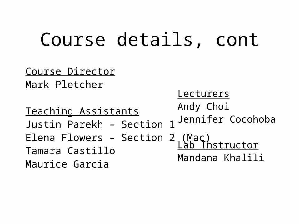
Course details, contCourse DirectorMark Pletcher

Teaching AssistantsJustin Parekh – Section 1Elena Flowers – Section 2 (Mac)Tamara CastilloMaurice Garcia

LecturersAndy ChoiJennifer Cocohoba

Lab InstructorMandana Khalili

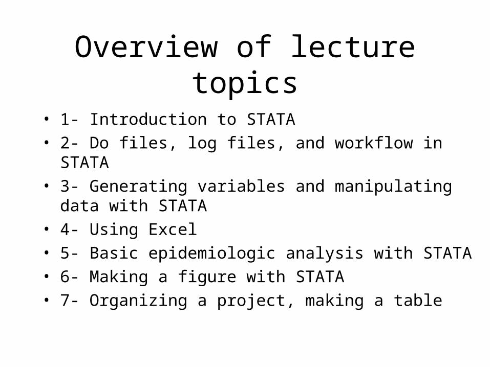
Overview of lecture topics

• 1- Introduction to STATA• 2- Do files, log files, and workflow in STATA• 3- Generating variables and manipulating data with STATA• 4- Using Excel• 5- Basic epidemiologic analysis with STATA• 6- Making a figure with STATA• 7- Organizing a project, making a table

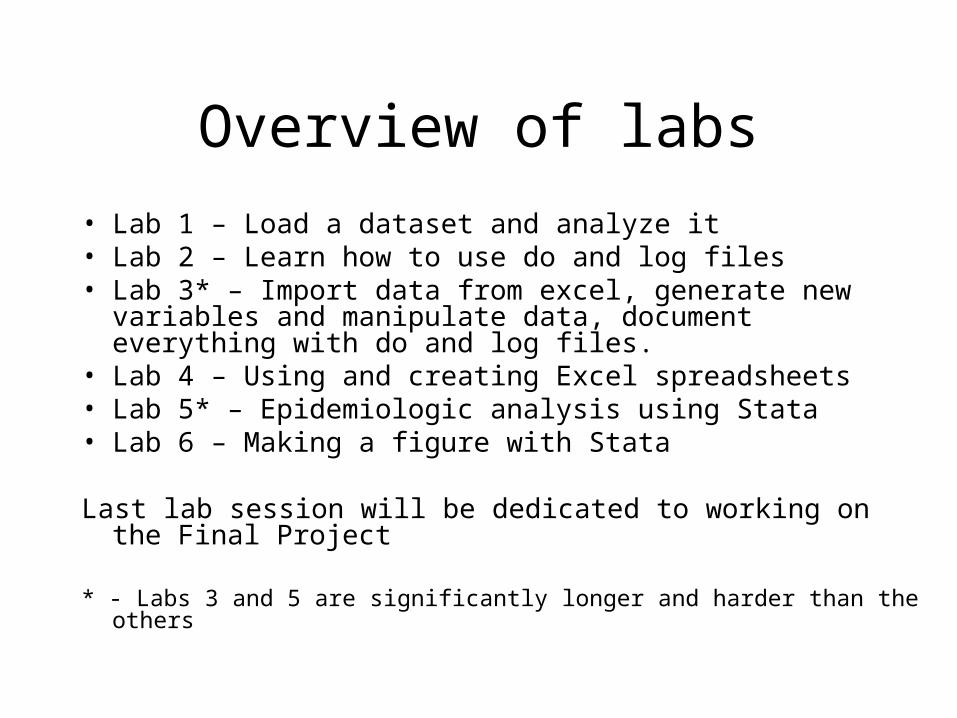
Overview of labs• Lab 1 – Load a dataset and analyze it• Lab 2 – Learn how to use do and log files• Lab 3* – Import data from excel, generate new variables and

manipulate data, document everything with do and log files.• Lab 4 – Using and creating Excel spreadsheets• Lab 5* – Epidemiologic analysis using Stata• Lab 6 – Making a figure with Stata

Last lab session will be dedicated to working on the Final Project

* - Labs 3 and 5 are significantly longer and harder than the others

Overview of labs, cont

• Official Lab time is 3:00-4:00, but we will start right after lecture, and you can leave when you are done.

Overview of labs, cont

• Labs are due the following week prior to lecture. Labs turned in late (less than 1 week) will receive only half credit; after that, no points will be awarded. However, ALL labs must be turned in to pass the class (even if no points are awarded).

• Lab 1 is paper• Labs 2-6 are electronic files, and should be emailed to your

section leader’s course email address: biostat212_section1@yahoo.com (Justin) or biostat212_section2@yahoo.com (Elena)

Final Project

• Create a Table and a Figure using your own data, document analysis using Stata.

• Due 1 week after last lab session, 20 points docked for each 1 day late.

Course Materials

• Course Overview• Final Project• Lectures and Labs (just in time)• Other handouts• Books

Getting started with STATA

Session 1

Types of software packages used in clinical research

• Statistical analysis packages• Spreadsheets• Database programs• Custom applications

– Cost-effectiveness analysis (TreeAge, etc)– Survey analysis (SUDAAN, etc)

Software packages for analyzing data

• STATA• SAS• S-plus, and R• SPS-S• SUDAAN• Epi-Info• JMP• MatLab• StatExact

Why use STATA?

• Quick start, user friendly• Immediate results, response• You can look at the data• Menu-driven option• Good graphics• Log and do files• Good manuals, help menu

Why NOT use STATA?

• SAS is used more often?• SAS does some things STATA does not• Programming easier with S-plus and R?• R is free• Complicated data structure and

manipulation easier with SAS?• Epi-info (free) is even easier than STATA?

STATA – Basic functionality

• Holds data for you– Stata holds 1 “flat” file dataset only (.dta file)

• Listens to what you want– Type a command, press enter

• Does stuff– Statistics, data manipulation, etc

• Shows you the results– Results window

Demo #1

• Open the program• Load some data• Look at it• Run a command

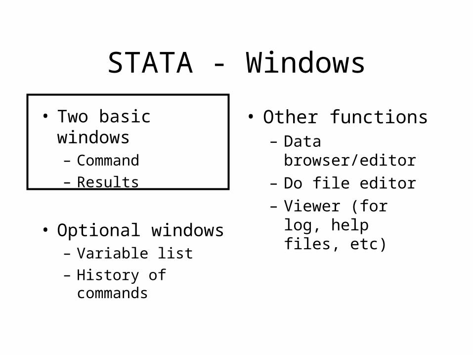
STATA - Windows

• Two basic windows– Command– Results

• Optional windows– Variable list– History of commands

• Other functions– Data browser/editor– Do file editor– Viewer (for log, help

files, etc)

STATA - Buttons

• The usual – open, save, print• Log-file open/suspend/close• Do-file editor• Browse and Edit• Break

STATA - Menus

• Almost every command can be accessed via menu

Demo #2

• Enter in some data• Look at it• Run a couple of commands

Menu vs. Command line

• Menu advantages– Look for commands you don’t know about– See the options for each command– Complex commands easier – learn syntax

• Command line advantages– Faster (if you know the command!)– “Closer” to the program– Only way to write “do” files

• Document and repeat analyses

STATA commandsDescribing your data

• describe [varlist]– Displays variable names, types, labels

• list [varlist]– Displays the values of all observations

• codebook [varlist]– Displays labels and codes for all variables

STATA commandsDescriptive statistics – continuous data

• summarize [varlist] [, detail]– # obs, mean, SD, range– “, detail” gets you more detail (median, etc)

• ci [varlist]– Mean, standard error of mean, and confidence intervals– Actually works for dichotomous variables, too.

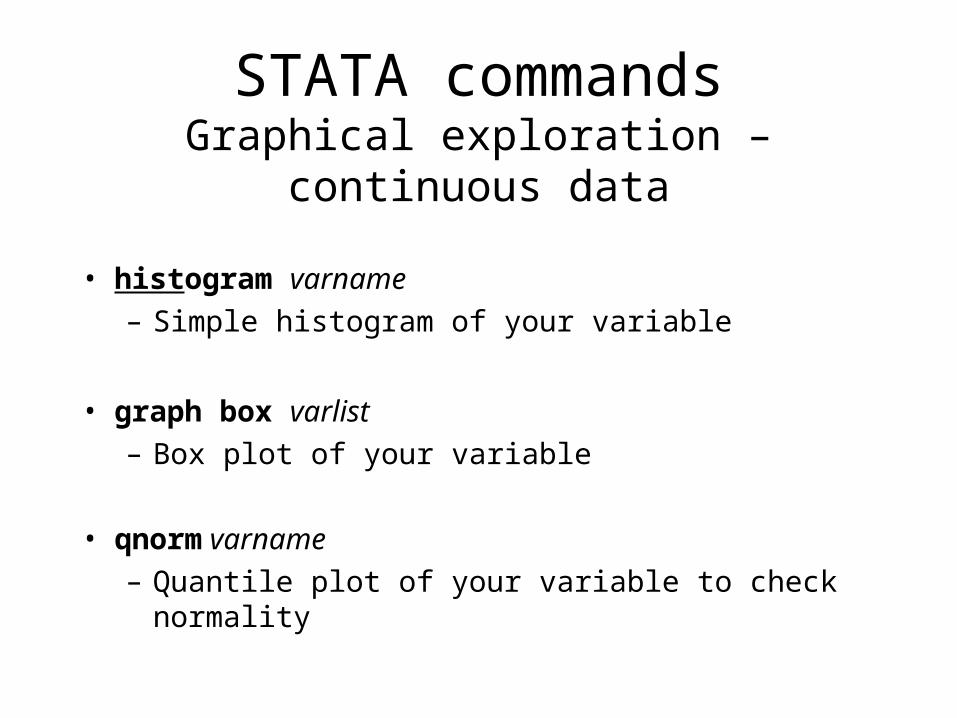
STATA commandsGraphical exploration – continuous data

• histogram varname– Simple histogram of your variable

• graph box varlist– Box plot of your variable

• qnorm varname– Quantile plot of your variable to check normality

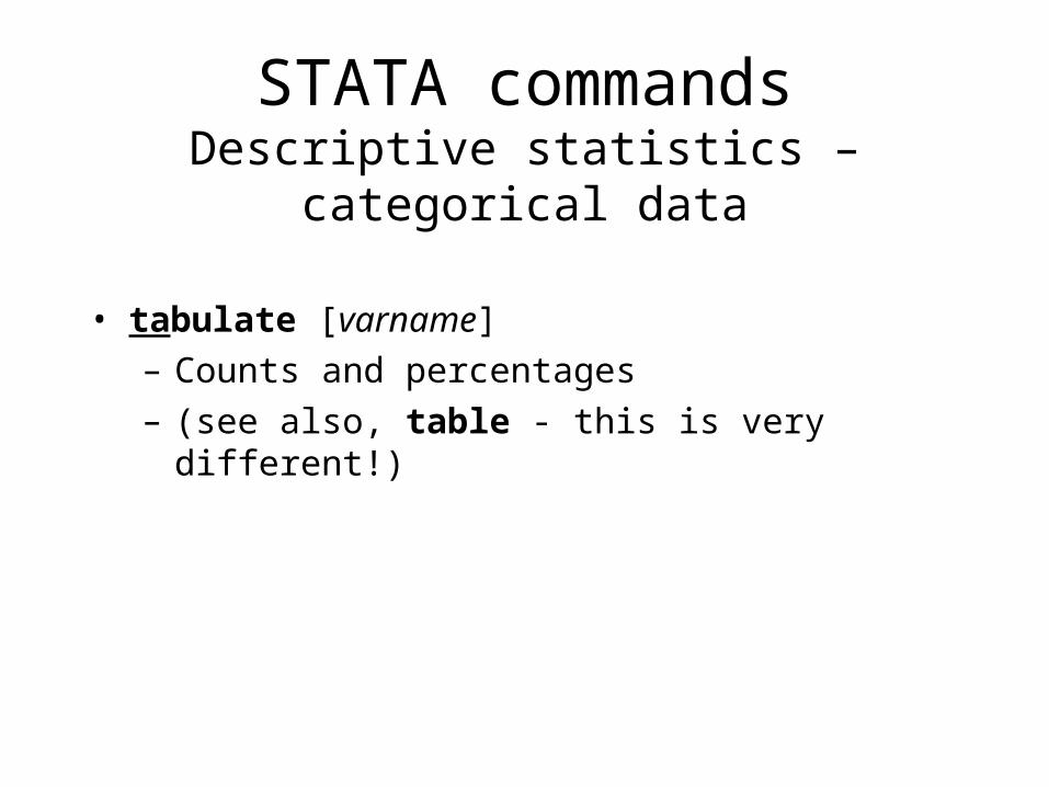
STATA commandsDescriptive statistics – categorical data

• tabulate [varname]– Counts and percentages– (see also, table - this is very different!)

STATA commandsAnalytic statistics – 2 categorical variables

STATA commandsAnalytic statistics – 2 categorical variables

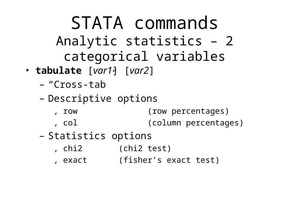
• tabulate [var1] [var2]– “Cross-tab”– Descriptive options

, row (row percentages), col (column percentages)

– Statistics options, chi2 (chi2 test), exact (fisher’s exact test)

Getting help

• Try to find the command on the pull-down menus

• Help menu– If you don’t know the command - Search...– If you know the command - Stata command...

• Try the manuals– more detail, theoretical underpinnings, etc

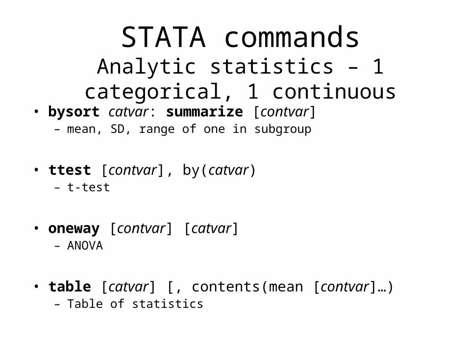
STATA commandsAnalytic statistics – 1 categorical, 1 continuous

STATA commandsAnalytic statistics – 1 categorical, 1 continuous

• bysort catvar: summarize [contvar]– mean, SD, range of one in subgroup

• ttest [contvar], by(catvar)– t-test

• oneway [contvar] [catvar]– ANOVA

• table [catvar] [, contents(mean [contvar]…)– Table of statistics

STATA commandsAnalytic statistics – 2 continuous

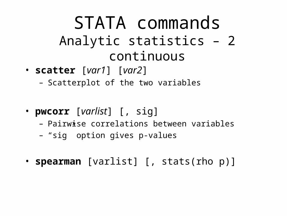
STATA commandsAnalytic statistics – 2 continuous

• scatter [var1] [var2]– Scatterplot of the two variables

• pwcorr [varlist] [, sig]– Pairwise correlations between variables– “sig” option gives p-values

• spearman [varlist] [, stats(rho p)]

Demo #3

• Load a STATA dataset• Explore the data• Describe the data• Answer some simple research questions

– Gender and HTN, age and HTN

In Lab Today…

• Familiarize yourself with Stata

• Load a dataset

• Use Stata commands to analyze data and fill in the blanks

Next week

• Do files, log files, and workflow in Stata

• Find a dataset!

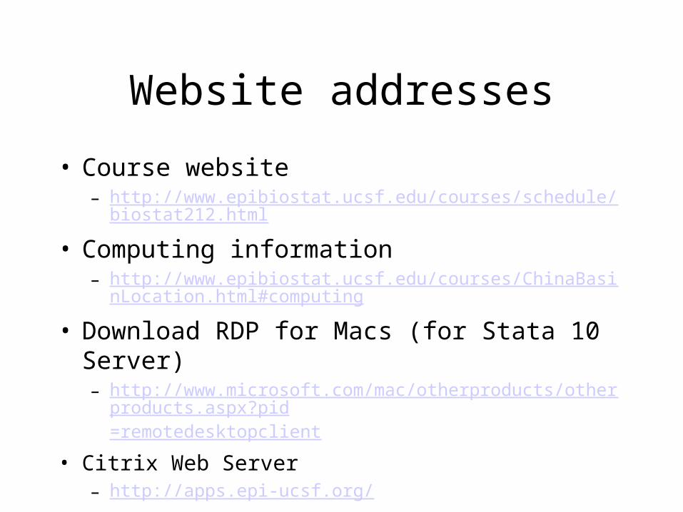
Website addresses

• Course website– http://www.epibiostat.ucsf.edu/courses/schedule/biostat212.html

• Computing information– http://www.epibiostat.ucsf.edu/courses/ChinaBasinLocation.html#

computing

• Download RDP for Macs (for Stata 10 Server)– http://www.microsoft.com/mac/otherproducts/otherproducts.aspx?

pid=remotedesktopclient

• Citrix Web Server– http://apps.epi-ucsf.org/