Embed Size (px)
Citation preview
MPI-BGC contribution to the CE Regional Experiment:
First Results and OutlookChristoph Gerbig
Max-Planck-Institute for Biogeochemistry Acknowledgements:
Bruno Neininger, Joel Giger, Han Bär (MetAir)
Stefan Körner, Armin Jordan, Michael Rothe (BGC)
Uwe Rascher, Heiner Geiss (FZJ)
Thorsten Warneke, Justus Notholt
MetAir
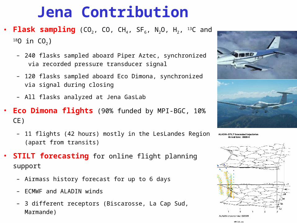
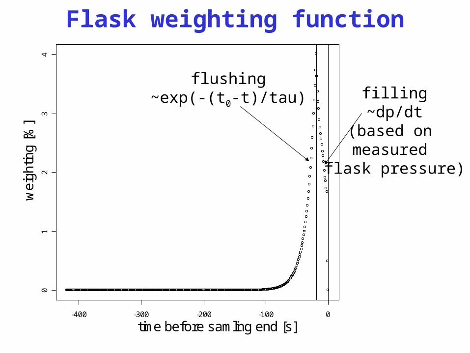
• Flask sampling (CO2, CO, CH4, SF6, N2O, H2, 13C and 18O in CO2)
– 240 flasks sampled aboard Piper Aztec, synchronized via recorded pressure transducer signal
– 120 flasks sampled aboard Eco Dimona, synchronized via signal during closing
– All flasks analyzed at Jena GasLab
• Eco Dimona flights (90% funded by MPI-BGC, 10%
CE)
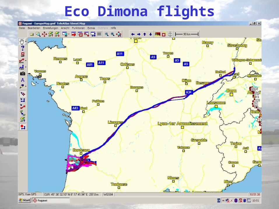
– 11 flights (42 hours) mostly in the LesLandes Region (apart from transits)
• STILT forecasting for online flight planning
support
– Airmass history forecast for up to 6 days
– ECMWF and ALADIN winds
– 3 different receptors (Biscarosse, La Cap Sud, Marmande)
Jena Contribution
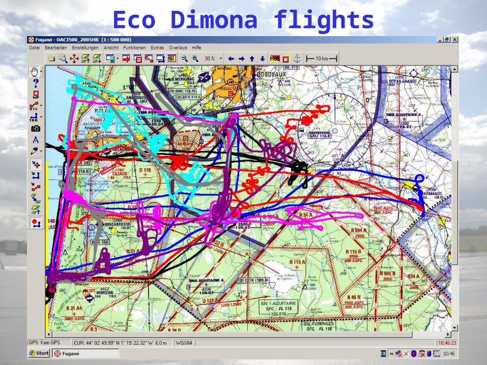
Eco Dimona flights
Eco Dimona flights
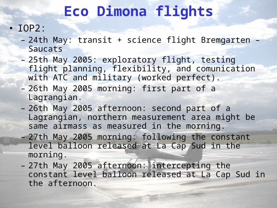
• IOP2:– 24th May: transit + science flight Bremgarten –
Saucats– 25th May 2005: exploratory flight, testing flight
planning, flexibility, and comunication with ATC and military (worked perfect).
– 26th May 2005 morning: first part of a Lagrangian.– 26th May 2005 afternoon: second part of a
Lagrangian, northern measurement area might be same airmass as measured in the morning.
– 27th May 2005 morning: following the constant level balloon released at La Cap Sud in the morning.
– 27th May 2005 afternoon: intercepting the constant level balloon released at La Cap Sud in the afternoon.
Eco Dimona flights

• IOP4:– 6th June: Lagrangian from North of Arcachon to La
Cap Sud, with help from constant level balloon released at La Cap Sud in the afternoon
– 7th June: Chasing the Bordeax plume towards the Biscarosse Tower, evidence of a sea breeze.
• IOP5:– 14th June: Lagrangian in a nearly ideal westerly
flow situation.– 15th June: Attempted Lagrangian under flow with
strong layering and windshear. This will be a critical test and a challenge for models. Radiation was reduced due to clouds (changed rtio direct/diffuse light).
– 17th June: transit + science flight Bremgarten – Saucats
Eco Dimona flights
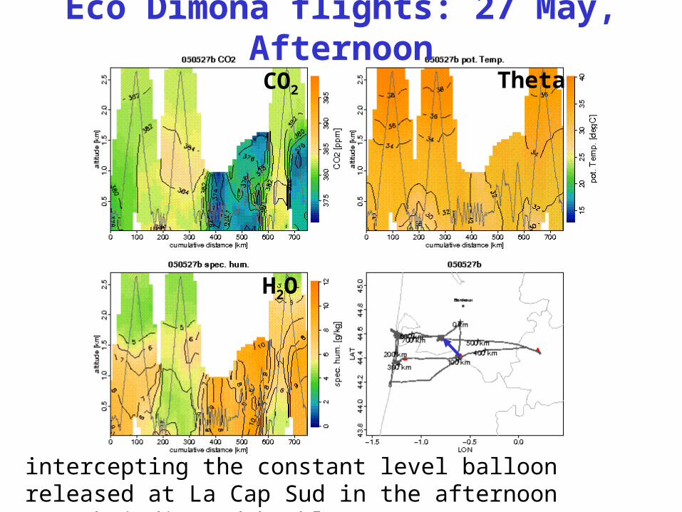
Eco Dimona flights: 27 May, Afternoon
CO2 Theta
H2O
intercepting the constant level balloon released at La Cap Sud in the afternoon (track indicated by blue arrow)
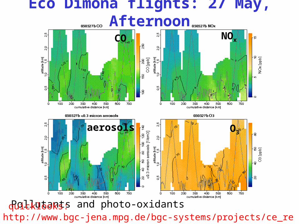
CO NOx
aerosols
Pollutants and photo-oxidants
Eco Dimona flights: 27 May, Afternoon
O3
quicklooks: http://www.bgc-jena.mpg.de/bgc-systems/projects/ce_re/xsection/
-400 -300 -200 -100 0
01
23
4
time before samling end [s]
we
igh
ting
[%]
piper6.6.2005a 32049Flask weighting function
-400 -300 -200 -100 0
01
23
time before samling end [s]
wei
ghtin
g [%
]
piper6.22.2005a 28250
-400 -300 -200 -100 0
01
23
4
time before samling end [s]
wei
ghtin
g [%
]
piper6.6.2005a 27163
-400 -300 -200 -100 0
01
23
time before samling end [s]
wei
ghtin
g [%
]
piper6.6.2005a 28015
-400 -300 -200 -100 0
01
23
time before samling end [s]
wei
ghtin
g [%
]
piper6.6.2005a 28624
-400 -300 -200 -100 0
0.0
1.0
2.0
3.0
time before samling end [s]
wei
ghtin
g [%
]
piper6.6.2005a 29517
-400 -300 -200 -100 0
01
23
4
time before samling end [s]
wei
ghtin
g [%
]
piper6.6.2005a 32049
-400 -300 -200 -100 0
01
23
45
67
time before samling end [s]
wei
ghtin
g [%
]
piper6.6.2005a 32349
-400 -300 -200 -100 0
01
23
45
time before samling end [s]
wei
ghtin
g [%
]
piper6.6.2005a 32847
-400 -300 -200 -100 0
01
23
4
time before samling end [s]
wei
ghtin
g [%
]
piper6.6.2005b 55513
-400 -300 -200 -100 0
01
23
time before samling end [s]
wei
ghtin
g [%
]
piper6.22.2005a 28250
-400 -300 -200 -100 0
01
23
4
time before samling end [s]
wei
ghtin
g [%
]
piper6.6.2005a 27163
-400 -300 -200 -100 0
01
23
time before samling end [s]
wei
ghtin
g [%
]
piper6.6.2005a 28015
-400 -300 -200 -100 0
01
23
time before samling end [s]
wei
ghtin
g [%
]
piper6.6.2005a 28624
-400 -300 -200 -100 0
0.0
1.0
2.0
3.0
time before samling end [s]
wei
ghtin
g [%
]
piper6.6.2005a 29517
-400 -300 -200 -100 0
01
23
4
time before samling end [s]
wei
ghtin
g [%
]
piper6.6.2005a 32049
-400 -300 -200 -100 0
01
23
45
67
time before samling end [s]
wei
ghtin
g [%
]
piper6.6.2005a 32349
-400 -300 -200 -100 0
01
23
45
time before samling end [s]
wei
ghtin
g [%
]
piper6.6.2005a 32847
-400 -300 -200 -100 0
01
23
4
time before samling end [s]
wei
ghtin
g [%
]
piper6.6.2005b 55513
flushing~exp(-(t0-t)/tau) filling
~dp/dt(based on measured
flask pressure)
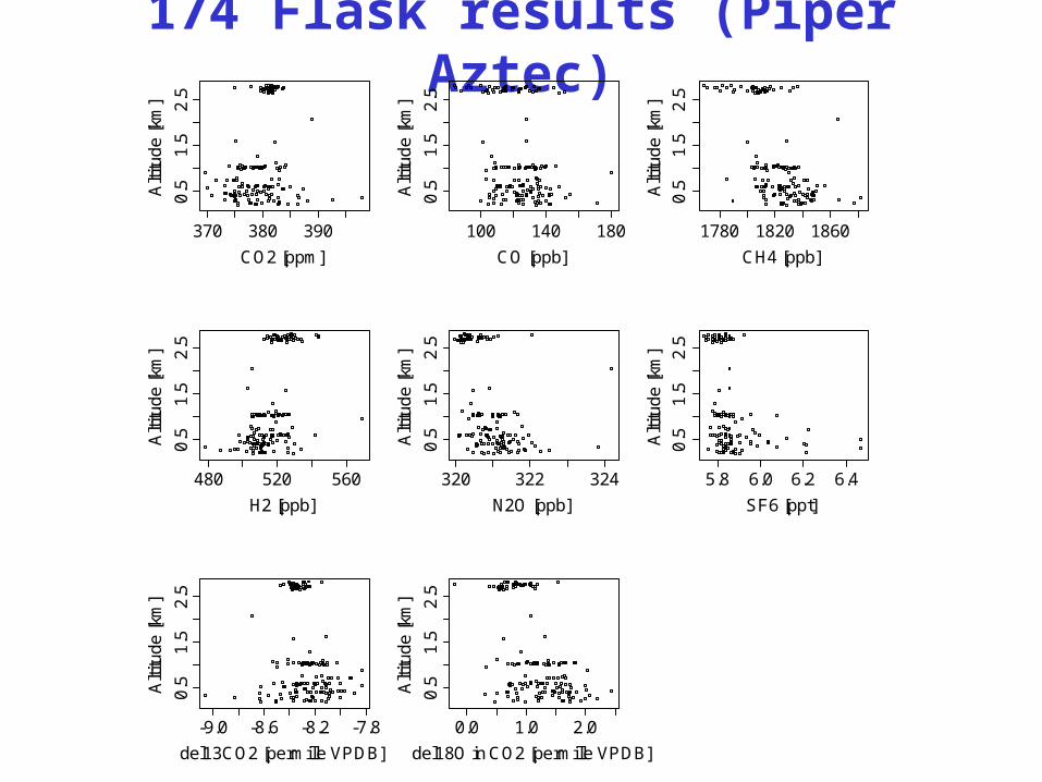
174 Flask results (Piper Aztec)
370 380 390
0.5
1.5
2.5
CO2 [ppm]
Alti
tud
e [k
m]
100 140 180
0.5
1.5
2.5
CO [ppb]
Alti
tud
e [k
m]
1780 1820 1860
0.5
1.5
2.5
CH4 [ppb]
Alti
tud
e [k
m]
480 520 560
0.5
1.5
2.5
H2 [ppb]
Alti
tud
e [k
m]
320 322 324
0.5
1.5
2.5
N2O [ppb]
Alti
tud
e [k
m]
5.8 6.0 6.2 6.4
0.5
1.5
2.5
SF6 [ppt]
Alti
tud
e [k
m]
-9.0 -8.6 -8.2 -7.8
0.5
1.5
2.5
del13CO2 [permille VPDB]
Alti
tud
e [k
m]
0.0 1.0 2.0
0.5
1.5
2.5
del18O in CO2 [permille VPDB]
Alti
tud
e [k
m]
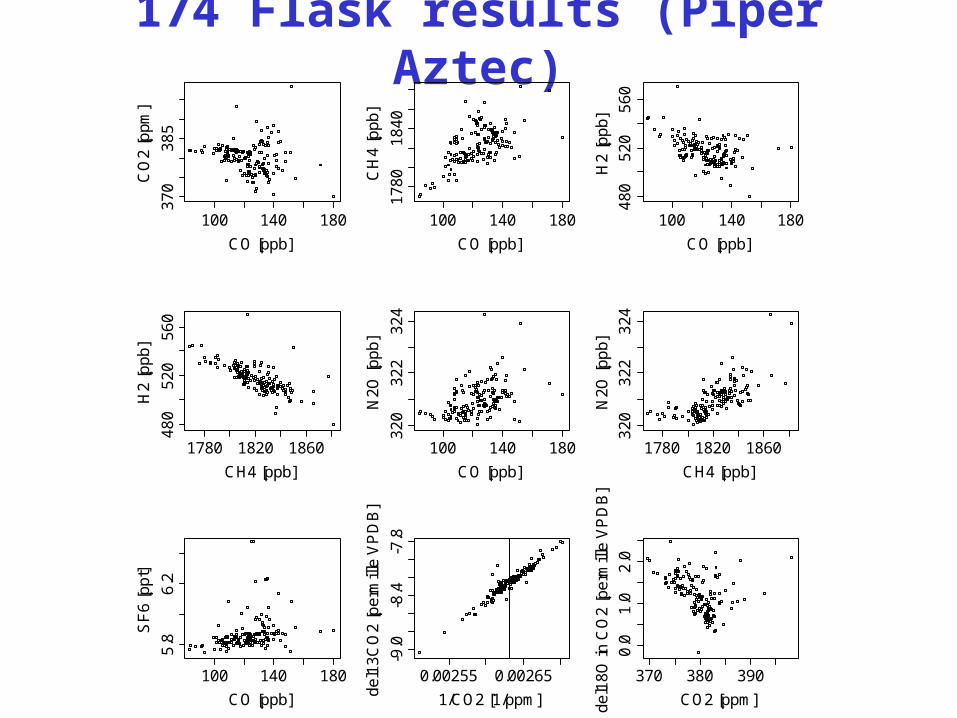
174 Flask results (Piper Aztec)
100 140 180
37
03
85
CO [ppb]
CO
2 [p
pm
]
100 140 180
17
80
18
40
CO [ppb]
CH
4 [p
pb
]
100 140 180
48
05
20
56
0
CO [ppb]
H2
[pp
b]
1780 1820 1860
48
05
20
56
0
CH4 [ppb]
H2
[pp
b]
100 140 180
32
03
22
32
4
CO [ppb]
N2
O [p
pb
]
1780 1820 1860
32
03
22
32
4
CH4 [ppb]
N2
O [p
pb
]
100 140 180
5.8
6.2
CO [ppb]
SF
6 [p
pt]
0.00255 0.00265
-9.0
-8.4
-7.8
1/CO2 [1/ppm]
de
l13
CO
2 [p
erm
ille
VP
DB
]
370 380 390
0.0
1.0
2.0
CO2 [ppm]de
l18
O in
CO
2 [p
erm
ille
VP
DB
]
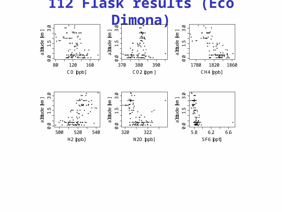
112 Flask results (Eco Dimona)
80 120 160
0.0
1.5
3.0
CO [ppb]
alti
tud
e [k
m]
370 380 390
0.0
1.5
3.0
CO2 [ppm]
alti
tud
e [k
m]
1780 1820 1860
0.0
1.5
3.0
CH4 [ppb]
alti
tud
e [k
m]
500 520 540
0.0
1.5
3.0
H2 [ppb]
alti
tud
e [k
m]
320 322
0.0
1.5
3.0
N2O [ppb]
alti
tud
e [k
m]
5.8 6.2 6.6
0.0
1.5
3.0
SF6 [ppt]
alti
tud
e [k
m]
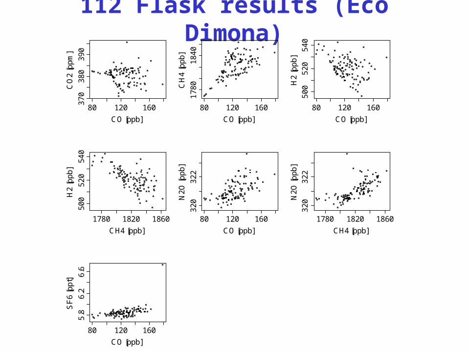
112 Flask results (Eco Dimona)
80 120 160
37
03
80
39
0
CO [ppb]
CO
2 [p
pm
]
80 120 160
17
80
18
40
CO [ppb]
CH
4 [p
pb
]
80 120 160
50
05
20
54
0
CO [ppb]
H2
[pp
b]
1780 1820 1860
50
05
20
54
0
CH4 [ppb]
H2
[pp
b]
80 120 160
32
03
22
CO [ppb]
N2
O [p
pb
]
1780 1820 1860
32
03
22
CH4 [ppb]
N2
O [p
pb
]
80 120 160
5.8
6.2
6.6
CO [ppb]
SF
6 [p
pt]
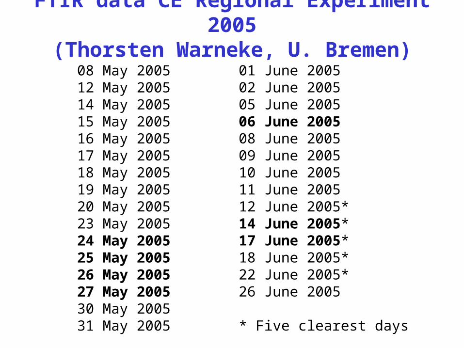
FTIR data CE Regional Experiment 2005
(Thorsten Warneke, U. Bremen)08 May 200512 May 200514 May 200515 May 200516 May 200517 May 200518 May 200519 May 200520 May 200523 May 200524 May 200525 May 200526 May 200527 May 200530 May 200531 May 2005
01 June 2005 02 June 2005 05 June 2005 06 June 2005 08 June 2005 09 June 2005 10 June 2005 11 June 2005 12 June 2005* 14 June 2005* 17 June 2005* 18 June 2005* 22 June 2005* 26 June 2005 * Five clearest days
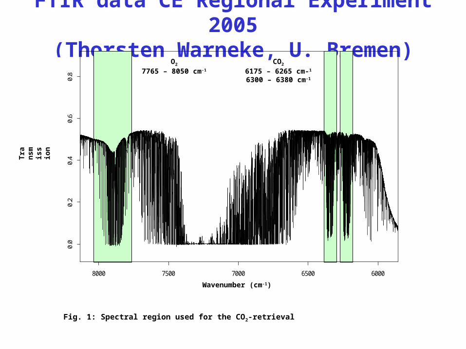
FTIR data CE Regional Experiment 2005
(Thorsten Warneke, U. Bremen)
\\Ftirserver\Ftir4\spectr14\02052200.0 Spitzbergen cm-1 5800.0 11000.0 cm-1 22/05/2002
60006500700075008000
Wavenumber cm-1
0.0
0.2
0.4
0.6
0.8
Sin
gle
chan
nel
CO2
6175 – 6265 cm-1
6300 – 6380 cm-1
O2
7765 – 8050 cm-1
Wavenumber (cm-1)
Tra
nsm
issi
on
Fig. 1: Spectral region used for the CO2-retrieval
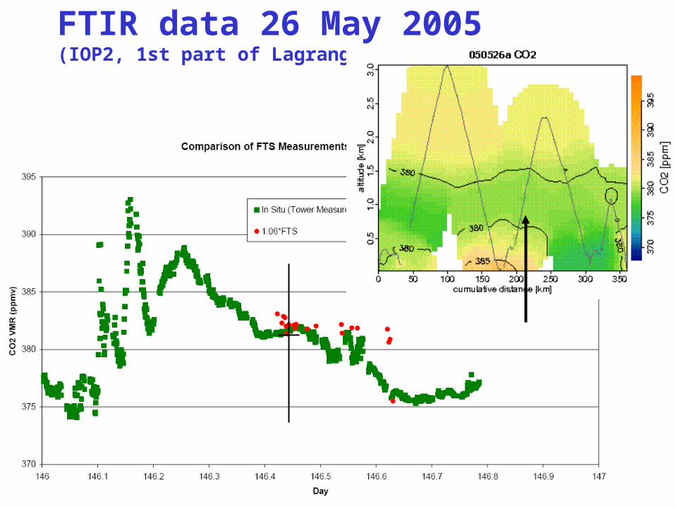
FTIR data 26 May 2005(IOP2, 1st part of Lagrangian)
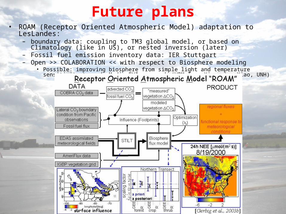
• ROAM (Receptor Oriented Atmospheric Model) adaptation to LesLandes: – boundary data: coupling to TM3 global model, or based on Climatology (like
in US), or nested inversion (later)– Fossil fuel emission inventory data: IER Stuttgart– Open >> COLABORATION << with respect to Biosphere modeling
• Possible: improving biosphere from simple light and temperature sensitivity towards Modis EVI approach (VPM from Xiangming Xiao, UNH)
Future plans
500 1500 2500 3500
500
1500
3000
radar zi [m]
stilt
zi [
m]
Orange
slope: 0.79
rsq: 0.09
500 1500 2500
500
1500
2500
radar zi [m]
stilt
zi [
m]
Pinnacle
slope: 0.97
rsq: 0.06
500 1500 2500
500
1500
2500
radar zi [m]
stilt
zi [
m]
Plymouth
slope: 0.99
rsq: 0.19
500 1500 2500
500
1500
2500
radar zi [m]
stilt
zi [
m]Schenectady
slope: 0.94
rsq: 0.38
500 1000 1500 2000
500
1500
radar zi [m]
stilt
zi [
m]
Appledore_Island
slope: 0.22
rsq: 0.13
500 1000 1500 2000
500
1500
radar zi [m]
stilt
zi [
m]
Concord
slope: 0.98
rsq: 0.03
500 1500 2500
500
1500
2500
radar zi [m]
stilt
zi [
m]
Pease_Tradeport
slope: 0.81
rsq: 0.08
local time [hr]
6 8 10 12 14 16
colorscale
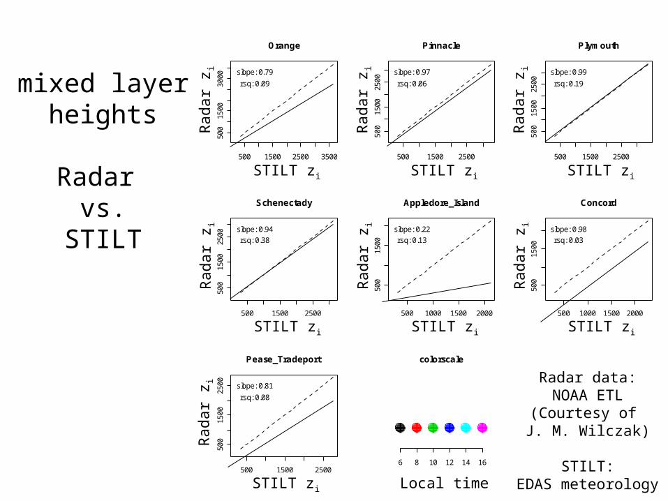
Comparison RADAR - STILT
RADAR data: NOAA ETL
(Courtesy of J. M. Wilczak)
mixed layerheights
Radar vs.
STILT
STILT zi
Radar
z i
STILT zi
Radar
z i
STILT zi
Radar
z i
STILT zi
Radar
z i
STILT zi
Radar
z i
STILT zi
Radar
z i
STILT zi
Radar
z i
Local time
Radar data:NOAA ETL
(Courtesy of J. M. Wilczak)
STILT:EDAS meteorology
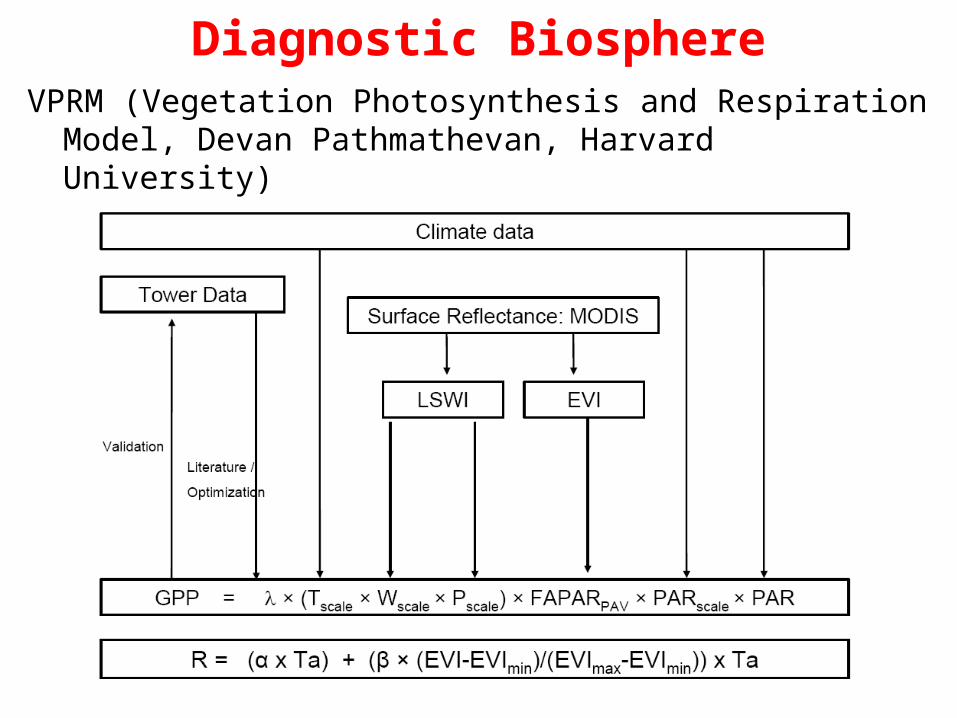
VPRM (Vegetation Photosynthesis and Respiration Model, Devan Pathmathevan, Harvard University)
-based on VPM from Xiangming Xiao, UNH
Diagnostic Biosphere
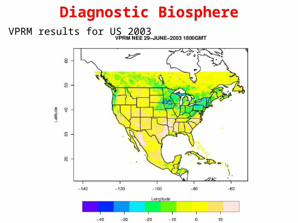
VPRM results for US 2003
Diagnostic Biosphere
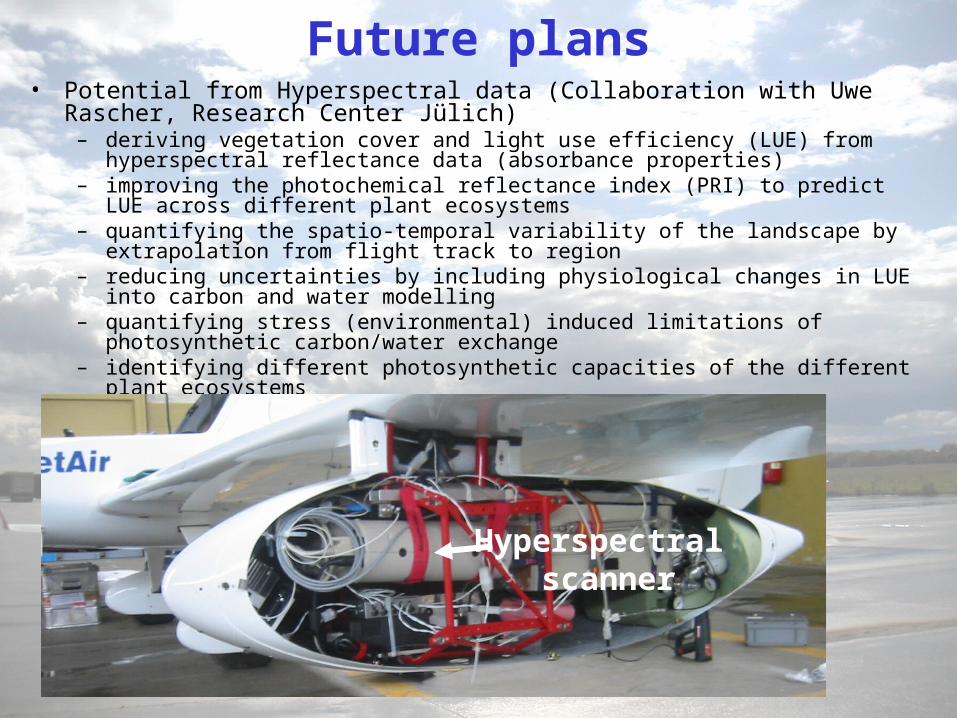
• Potential from Hyperspectral data (Collaboration with Uwe Rascher, Research Center Jülich)– deriving vegetation cover and light use efficiency (LUE) from hyperspectral
reflectance data (absorbance properties)– improving the photochemical reflectance index (PRI) to predict LUE across
different plant ecosystems– quantifying the spatio-temporal variability of the landscape by extrapolation
from flight track to region– reducing uncertainties by including physiological changes in LUE into carbon
and water modelling– quantifying stress (environmental) induced limitations of photosynthetic
carbon/water exchange– identifying different photosynthetic capacities of the different plant
ecosystems
Future plans
Hyperspectral scanner
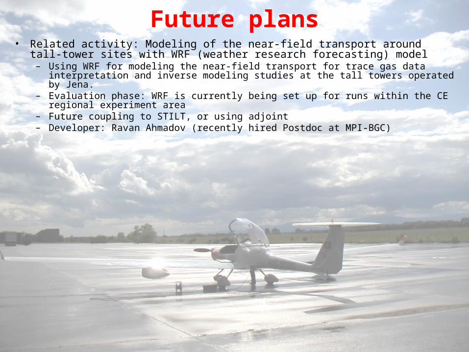
• Related activity: Modeling of the near-field transport around tall-tower sites with WRF (weather research forecasting) model – Using WRF for modeling the near-field transport for trace gas data
interpretation and inverse modeling studies at the tall towers operated by Jena. – Evaluation phase: WRF is currently being set up for runs within the CE regional
experiment area– Future coupling to STILT, or using adjoint– Developer: Ravan Ahmadov (recently hired Postdoc at MPI-BGC)
Future plans
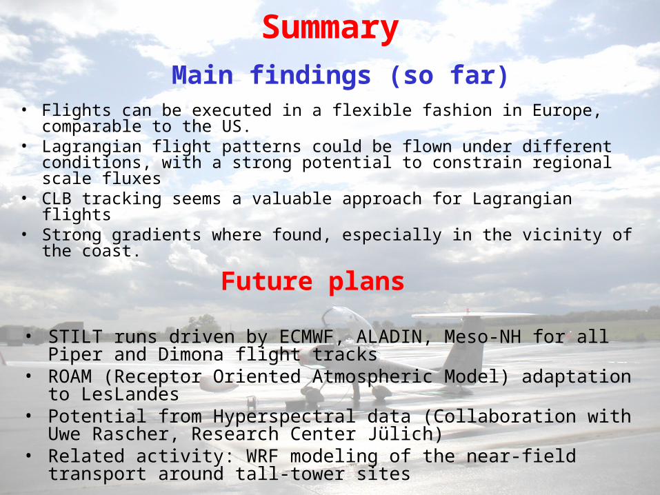
• STILT runs driven by ECMWF, ALADIN, Meso-NH for all Piper and Dimona flight tracks
• ROAM (Receptor Oriented Atmospheric Model) adaptation to LesLandes
• Potential from Hyperspectral data (Collaboration with Uwe Rascher, Research Center Jülich)
• Related activity: WRF modeling of the near-field transport around tall-tower sites
Summary
Future plans
• Flights can be executed in a flexible fashion in Europe, comparable to the US.
• Lagrangian flight patterns could be flown under different conditions, with a strong potential to constrain regional scale fluxes
• CLB tracking seems a valuable approach for Lagrangian flights• Strong gradients where found, especially in the vicinity of the
coast.
Main findings (so far)
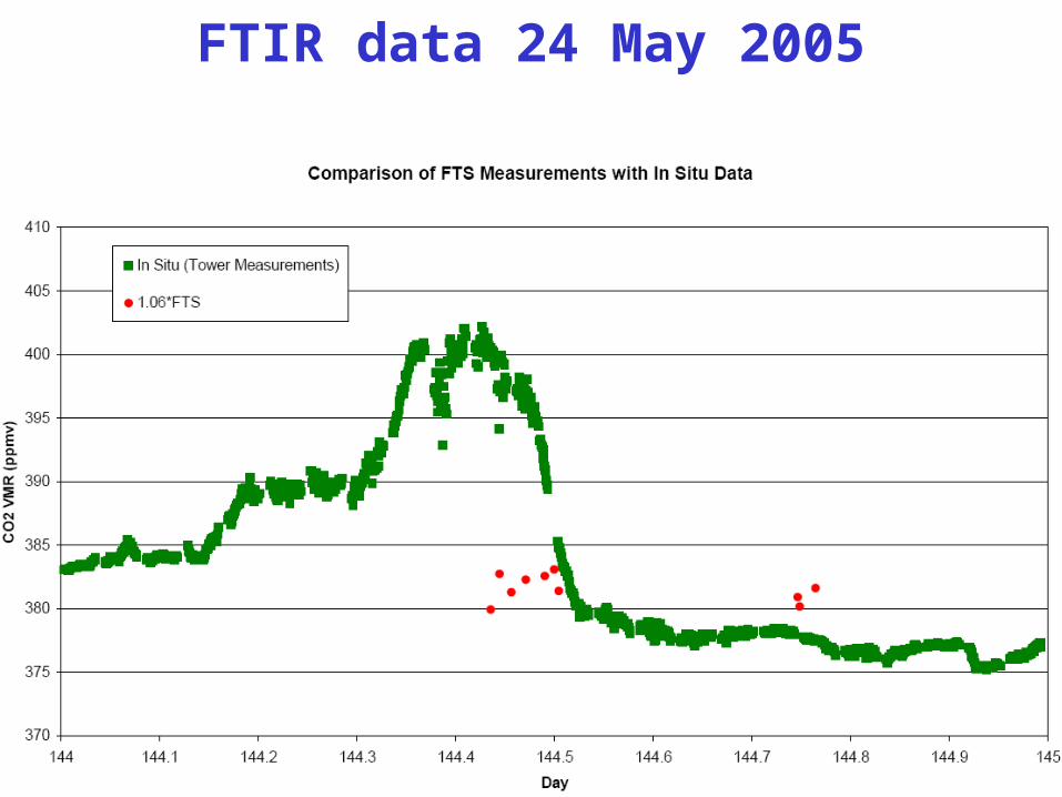
FTIR data 24 May 2005
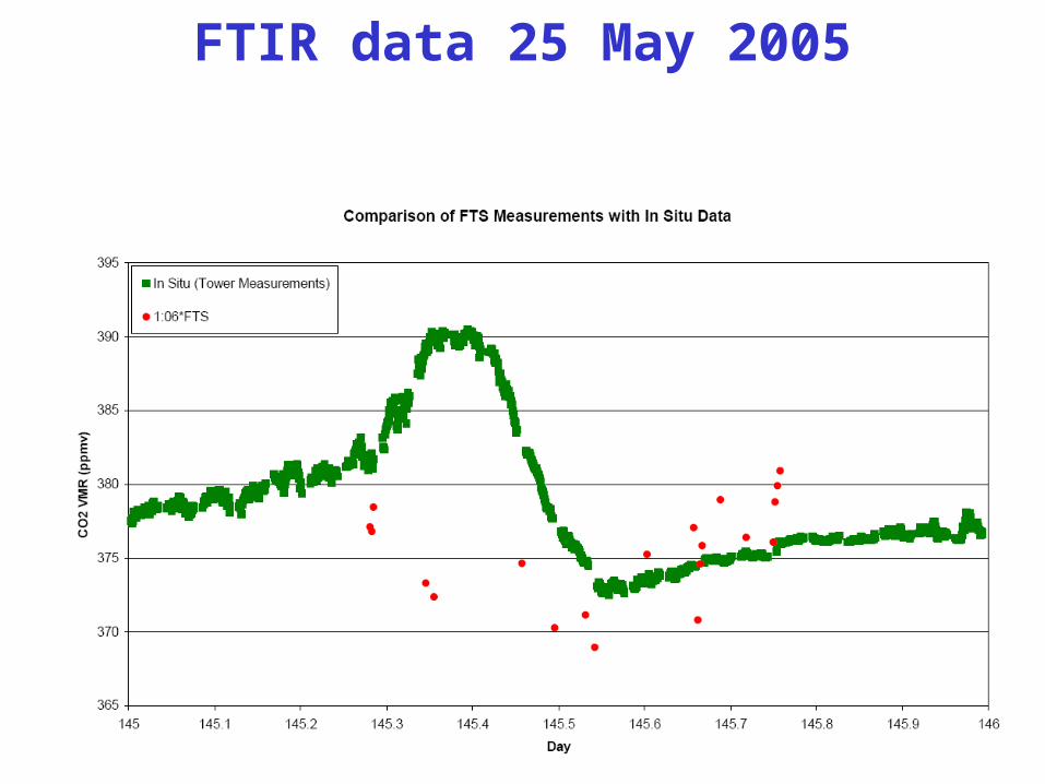
FTIR data 25 May 2005
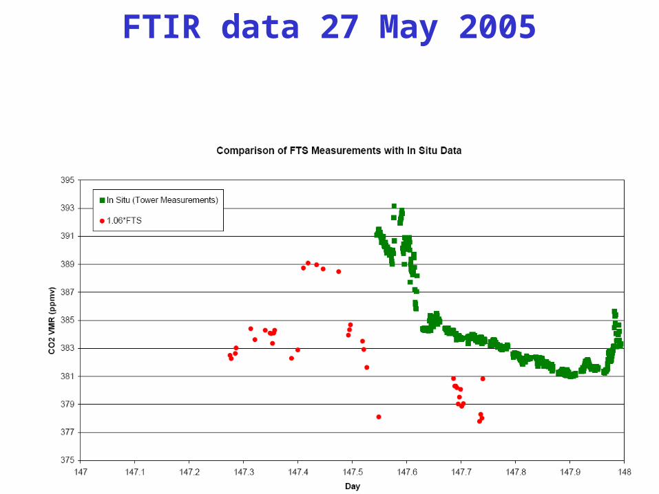
FTIR data 27 May 2005
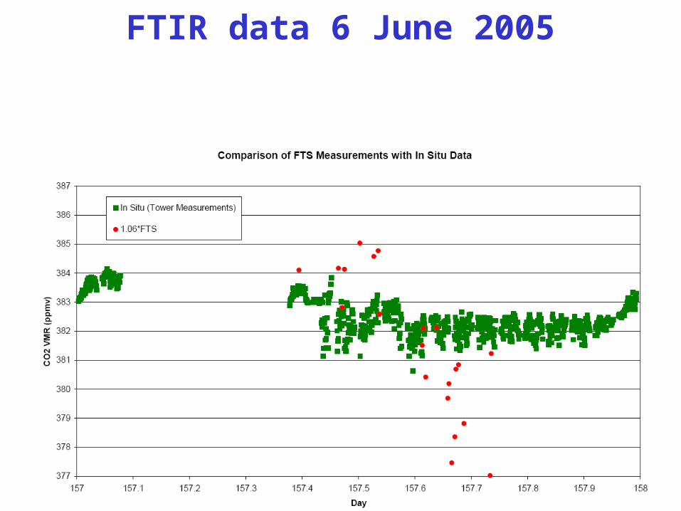
FTIR data 6 June 2005
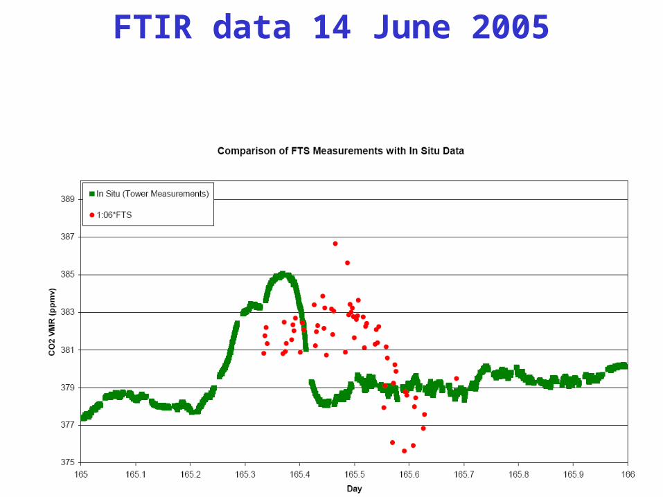
FTIR data 14 June 2005
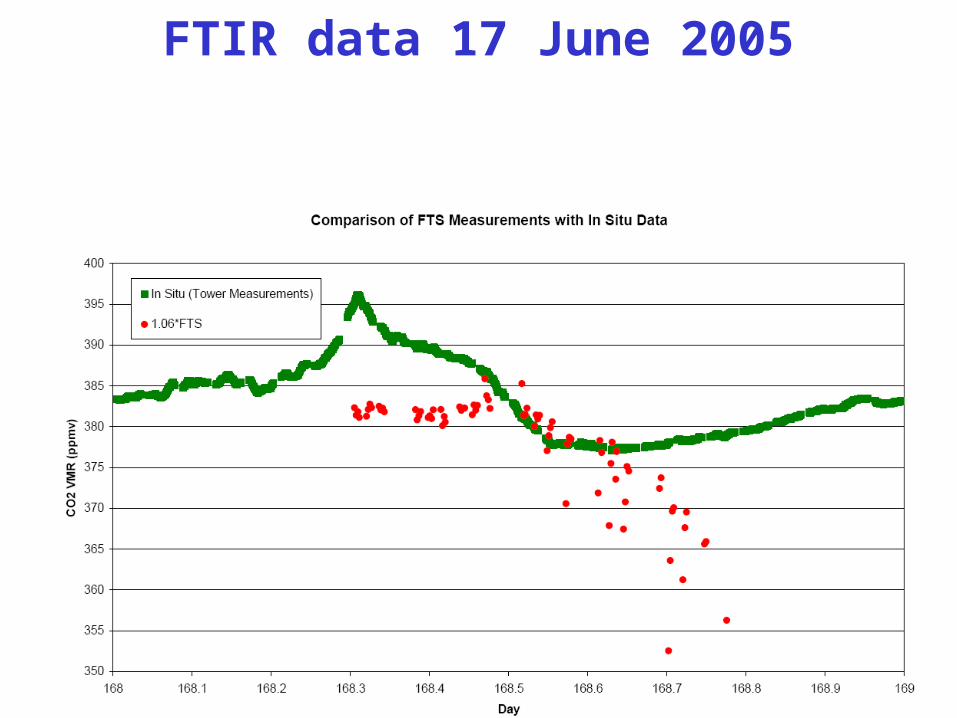
FTIR data 17 June 2005
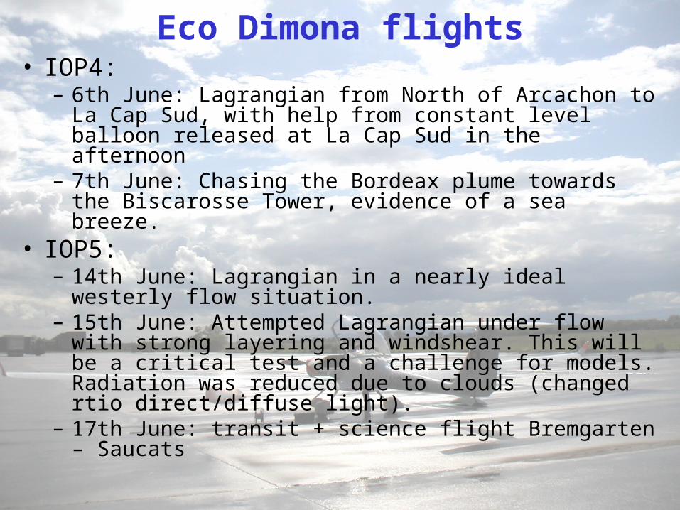
• IOP4:– 6th June: Lagrangian from North of Arcachon to La
Cap Sud, with help from constant level balloon released at La Cap Sud in the afternoon
– 7th June: Chasing the Bordeax plume towards the Biscarosse Tower, evidence of a sea breeze.
• IOP5:– 14th June: Lagrangian in a nearly ideal westerly
flow situation.– 15th June: Attempted Lagrangian under flow with
strong layering and windshear. This will be a critical test and a challenge for models. Radiation was reduced due to clouds (changed rtio direct/diffuse light).
– 17th June: transit + science flight Bremgarten – Saucats
Eco Dimona flights
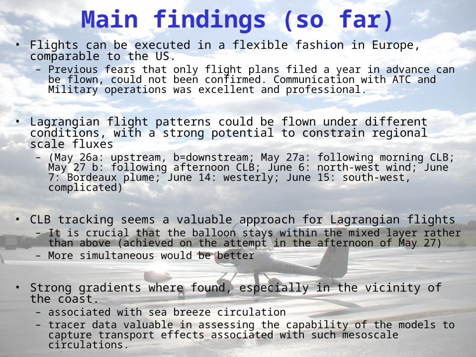
• Flights can be executed in a flexible fashion in Europe, comparable to the US. – Previous fears that only flight plans filed a year in advance can be
flown, could not been confirmed. Communication with ATC and Military operations was excellent and professional.
• Lagrangian flight patterns could be flown under different conditions, with a strong potential to constrain regional scale fluxes– (May 26a: upstream, b=downstream; May 27a: following morning CLB;
May 27 b: following afternoon CLB; June 6: north-west wind; June 7: Bordeaux plume; June 14: westerly; June 15: south-west, complicated)
• CLB tracking seems a valuable approach for Lagrangian flights– It is crucial that the balloon stays within the mixed layer rather than
above (achieved on the attempt in the afternoon of May 27)– More simultaneous would be better
• Strong gradients where found, especially in the vicinity of the coast.– associated with sea breeze circulation– tracer data valuable in assessing the capability of the models to
capture transport effects associated with such mesoscale circulations.
Main findings (so far)


![[CM2015] Chapter 7 - Biogeochemistry](https://img.pdfslide.net/doc/110x75/589f959c1a28ab1b198b6265/cm2015-chapter-7-biogeochemistry.jpg)