Embed Size (px)
Citation preview
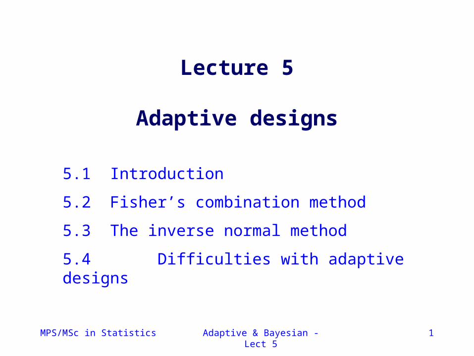
MPS/MSc in Statistics Adaptive & Bayesian - Lect 5 1
Lecture 5
Adaptive designs
5.1 Introduction
5.2 Fisher’s combination method
5.3 The inverse normal method
5.4 Difficulties with adaptive designs
MPS/MSc in Statistics Adaptive & Bayesian - Lect 5 2
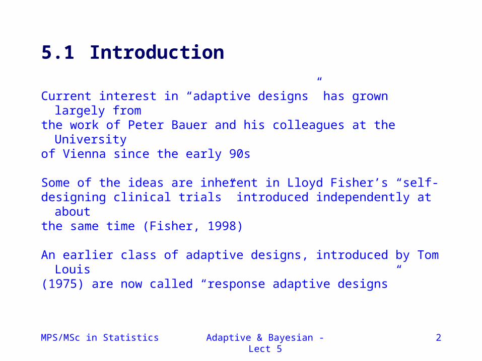
5.1 Introduction
Current interest in “adaptive designs” has grown largely fromthe work of Peter Bauer and his colleagues at the Universityof Vienna since the early 90s
Some of the ideas are inherent in Lloyd Fisher’s “self-designing clinical trials” introduced independently at about the same time (Fisher, 1998)
An earlier class of adaptive designs, introduced by Tom Louis
(1975) are now called “response adaptive designs”
MPS/MSc in Statistics Adaptive & Bayesian - Lect 5 3
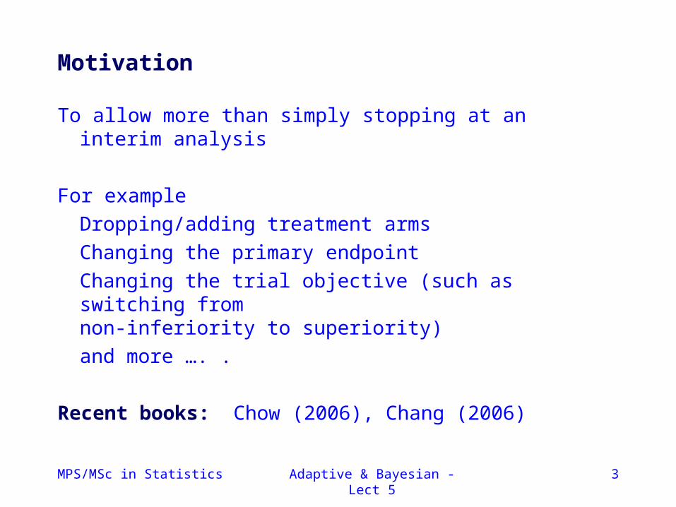
Motivation
To allow more than simply stopping at an interim analysis
For example
Dropping/adding treatment arms
Changing the primary endpoint
Changing the trial objective (such as switching fromnon-inferiority to superiority)
and more …. .
Recent books: Chow (2006), Chang (2006)
MPS/MSc in Statistics Adaptive & Bayesian - Lect 5 4
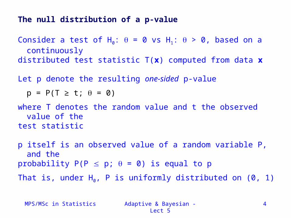
The null distribution of a p-value
Consider a test of H0: = 0 vs H1: > 0, based on a continuouslydistributed test statistic T(x) computed from data x
Let p denote the resulting one-sided p-value
p = P(T ≥ t; = 0)
where T denotes the random value and t the observed value of thetest statistic
p itself is an observed value of a random variable P, and theprobability P(P p; = 0) is equal to p
That is, under H0, P is uniformly distributed on (0, 1)
MPS/MSc in Statistics Adaptive & Bayesian - Lect 5 5
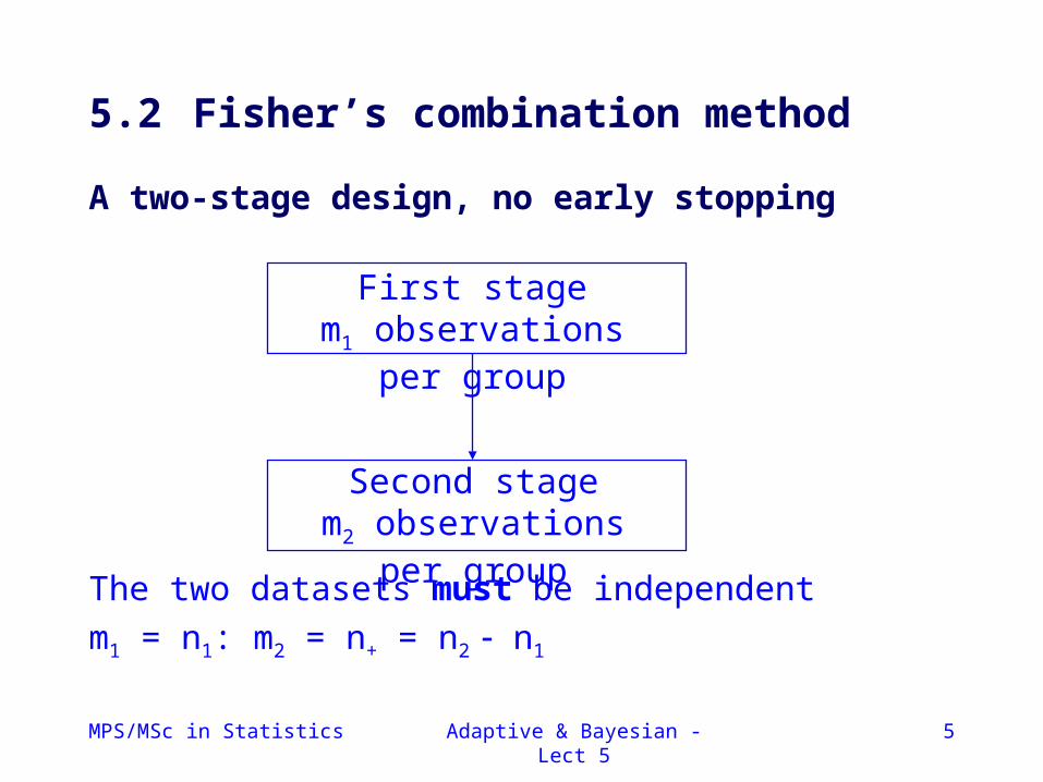
5.2 Fisher’s combination method
A two-stage design, no early stopping
The two datasets must be independent
m1 = n1: m2 = n+ = n2 n1
First stagem1 observations per group
Second stagem2 observations per group
MPS/MSc in Statistics Adaptive & Bayesian - Lect 5 6
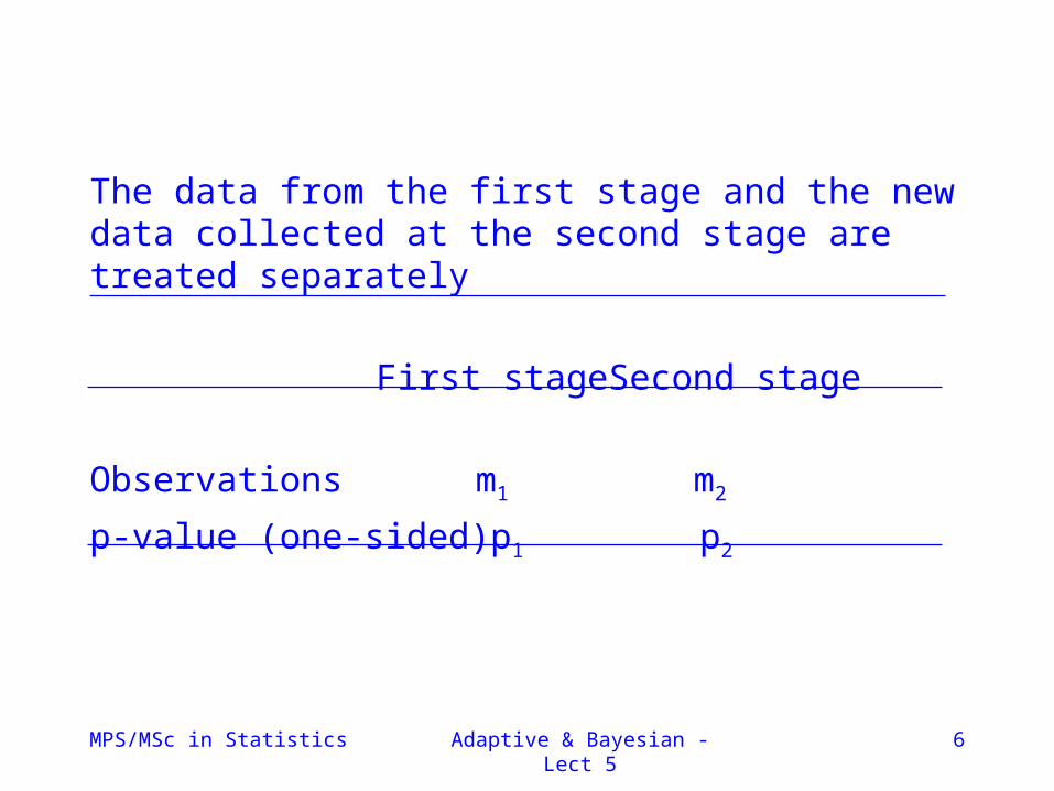
The data from the first stage and the new data collected at the second stage are treated separately
First stage Second stage
Observations m1 m2
p-value (one-sided) p1 p2
MPS/MSc in Statistics Adaptive & Bayesian - Lect 5 7
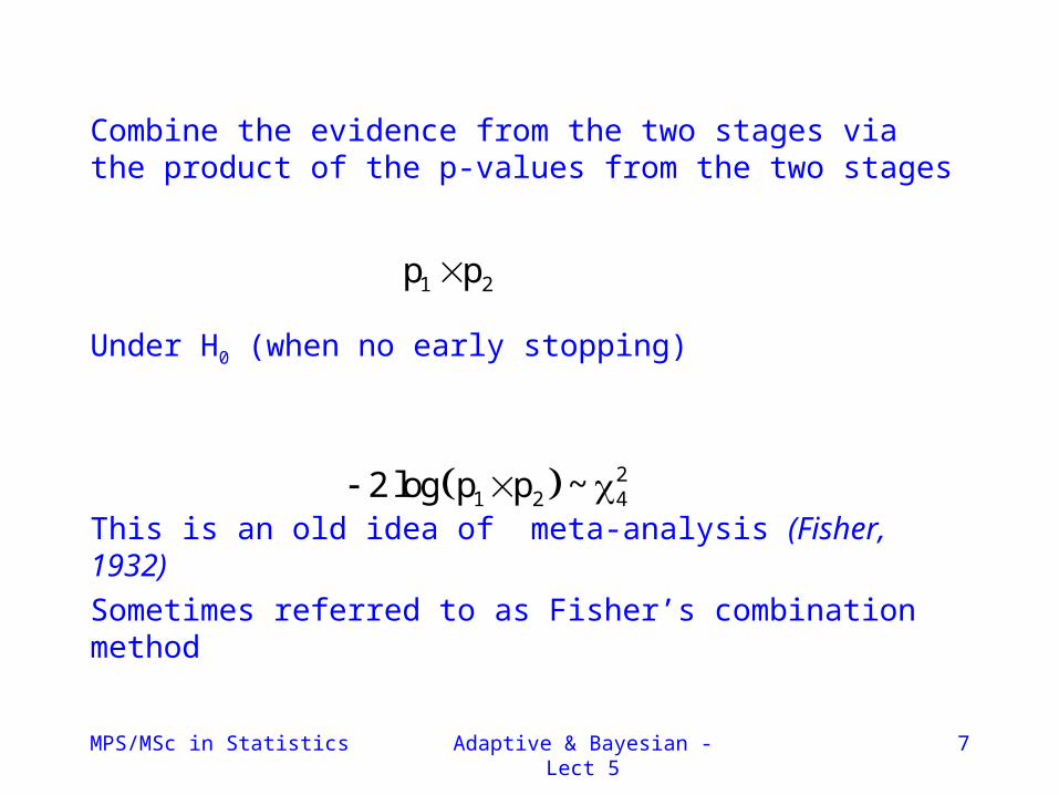
Combine the evidence from the two stages via the product of the p-values from the two stages
Under H0 (when no early stopping)
This is an old idea of meta-analysis (Fisher, 1932)
Sometimes referred to as Fisher’s combination method
1 2p p
21 2 42 log p p ~
MPS/MSc in Statistics Adaptive & Bayesian - Lect 5 8
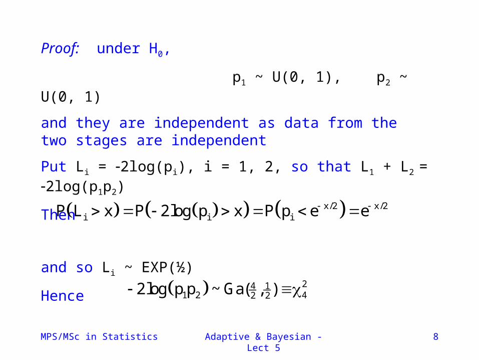
Proof: under H0,
p1 ~ U(0, 1), p2 ~ U(0, 1)
and they are independent as data from the two stages are independent
Put Li = 2log(pi), i = 1, 2, so that L1 + L2 = 2log(p1p2)
Then
and so Li ~ EXP(½)
Hence
x/2 x/2i i iP L x P 2log p x P p e e
24 11 2 42 22log p p ~ Ga( , )
MPS/MSc in Statistics Adaptive & Bayesian - Lect 5 9
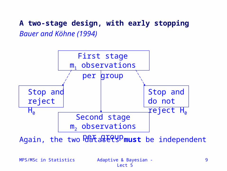
A two-stage design, with early stopping
Bauer and Köhne (1994)
Again, the two datasets must be independent
First stagem1 observations per group
Second stagem2 observations per group
Stop and reject H0
Stop and do not reject H0
MPS/MSc in Statistics Adaptive & Bayesian - Lect 5 10
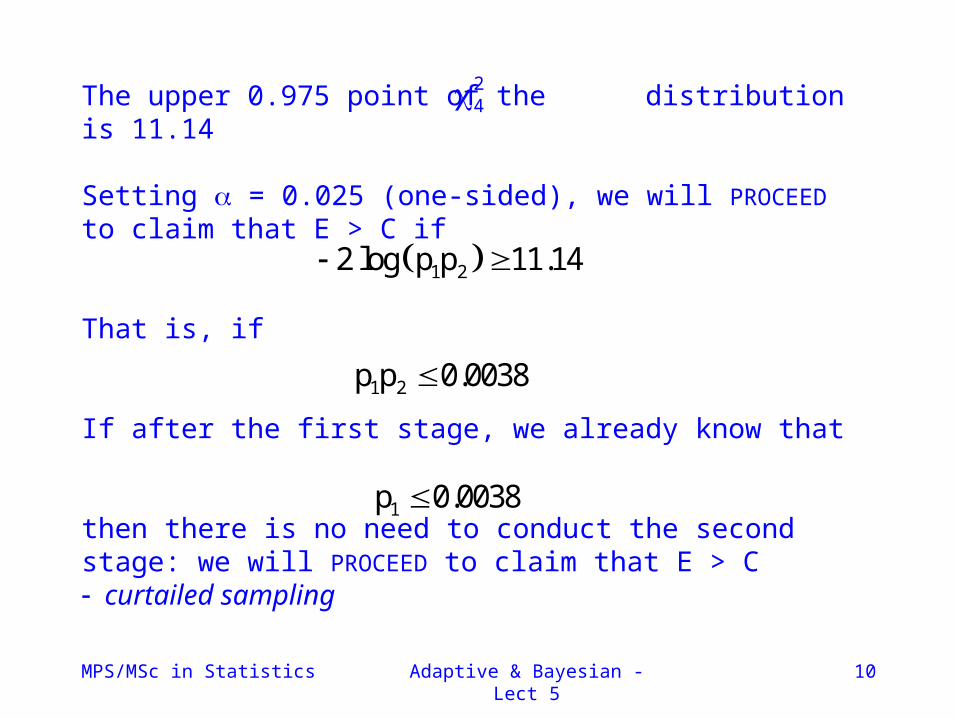
The upper 0.975 point of the distribution is 11.14
Setting = 0.025 (one-sided), we will PROCEED to claim that E > C if
That is, if
If after the first stage, we already know that
then there is no need to conduct the second stage: we will PROCEED to claim that E > C curtailed sampling
1 22 log p p 11.14
24
1 2p p 0.0038
1p 0.0038
MPS/MSc in Statistics Adaptive & Bayesian - Lect 5 11
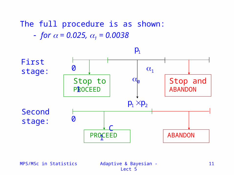
The full procedure is as shown:
for = 0.025, 1 = 0.0038
Stop to PROCEED
Stop and ABANDON
PROCEED ABANDON
1p
0 1 0 1
1 2p p
0 C 1Second stage:
First stage:
MPS/MSc in Statistics Adaptive & Bayesian - Lect 5 12
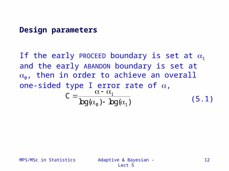
Design parameters
If the early PROCEED boundary is set at 1 and the early ABANDON boundary is set at 0, then in order to achieve an overall one-sided type I error rate of ,
1
0 1
Clog( ) log( )
(5.1)
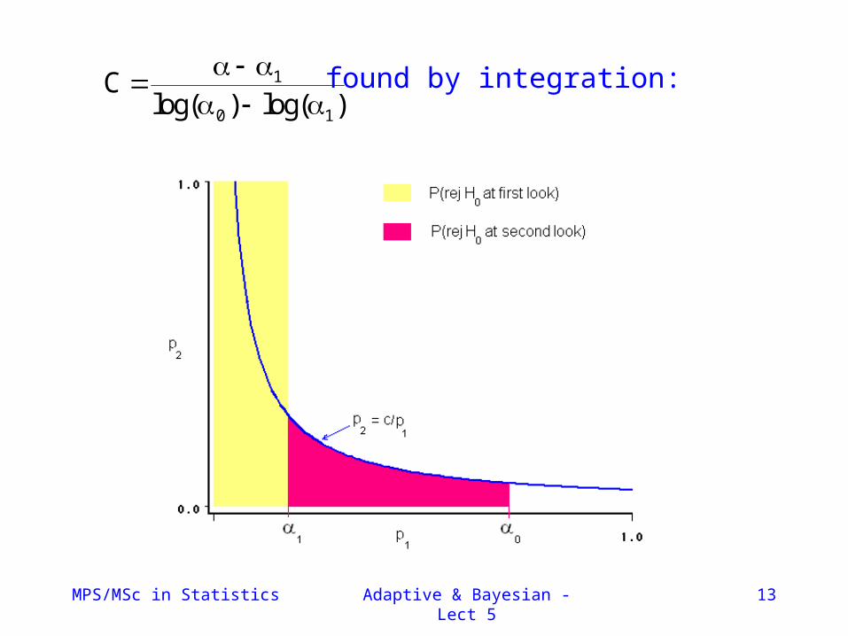
MPS/MSc in Statistics Adaptive & Bayesian - Lect 5 13
1
0 1
Clog( ) log( )
found by integration:
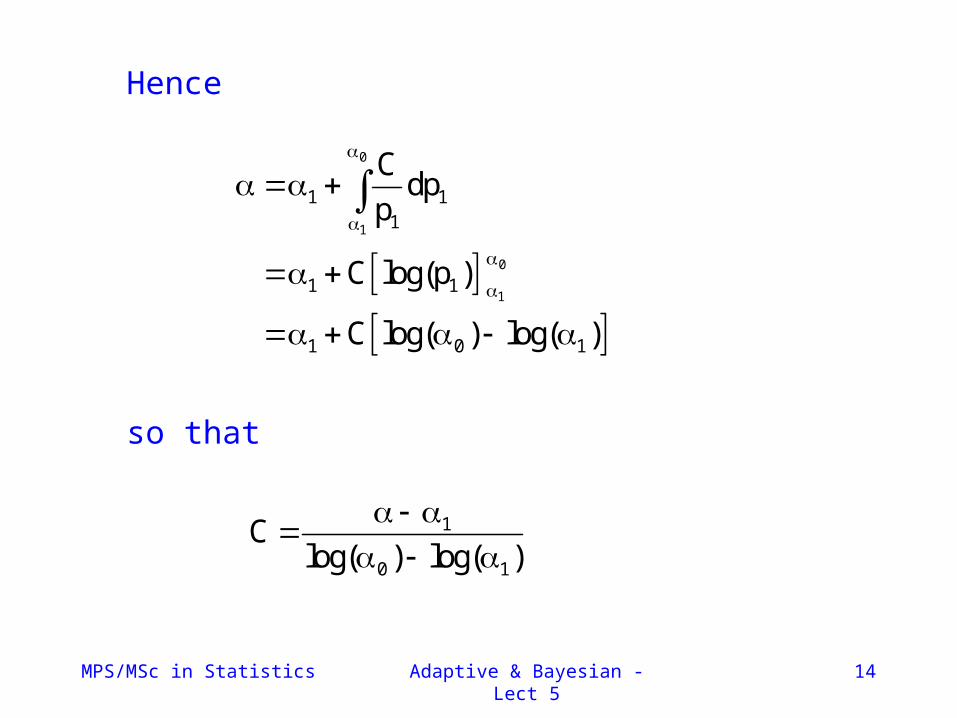
MPS/MSc in Statistics Adaptive & Bayesian - Lect 5 14
0
1
0
1
1 11
1 1
1 0 1
Cdp
p
C log(p )
C log( ) log( )
1
0 1
Clog( ) log( )
Hence
so that
MPS/MSc in Statistics Adaptive & Bayesian - Lect 5 15
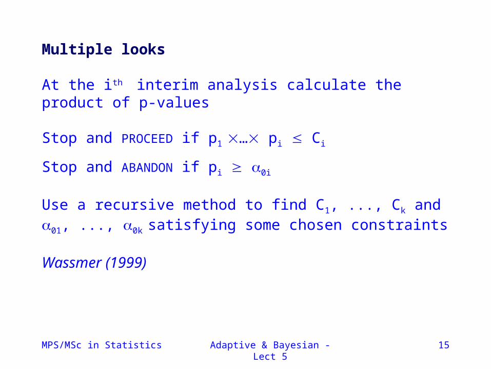
Multiple looks
At the ith interim analysis calculate the product of p-values
Stop and PROCEED if p1 … pi Ci
Stop and ABANDON if pi 0i
Use a recursive method to find C1, ..., Ck and 01, ..., 0k
satisfying some chosen constraints
Wassmer (1999)
MPS/MSc in Statistics Adaptive & Bayesian - Lect 5 16
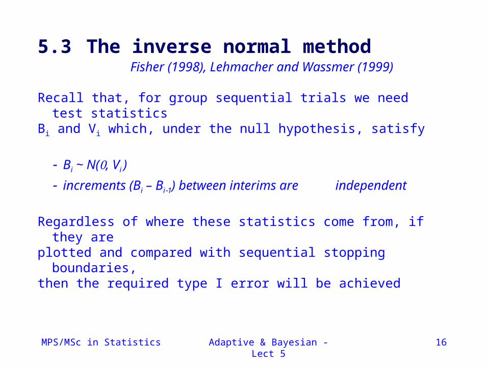
Fisher (1998), Lehmacher and Wassmer (1999)
Recall that, for group sequential trials we need test statisticsBi and Vi which, under the null hypothesis, satisfy
Bi ~ N(, Vi )
increments (Bi – Bi1) between interims are independent
Regardless of where these statistics come from, if they areplotted and compared with sequential stopping boundaries,then the required type I error will be achieved
5.3 The inverse normal method
MPS/MSc in Statistics Adaptive & Bayesian - Lect 5 17
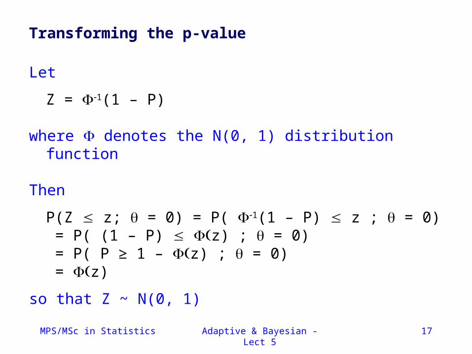
Transforming the p-value
Let
Z = 1(1 – P)
where denotes the N(0, 1) distribution function
Then
P(Z z; = 0) = P( 1(1 – P) z ; = 0) = P( (1 – P) z) ; = 0) = P( P ≥ 1 – z) ; = 0) = z)
so that Z ~ N(0, 1)
MPS/MSc in Statistics Adaptive & Bayesian - Lect 5 18
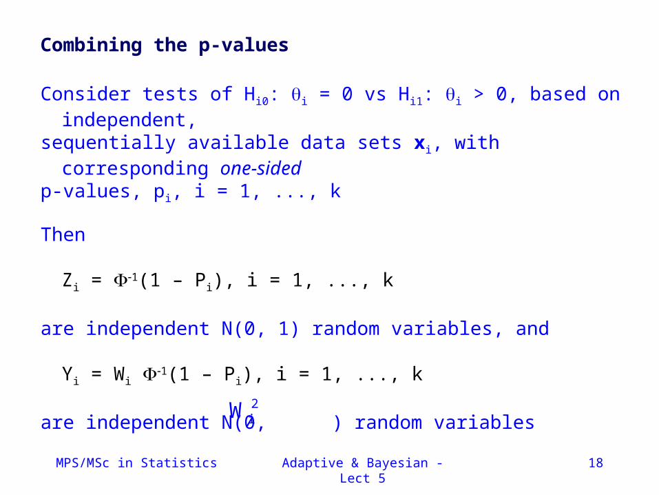
Combining the p-values
Consider tests of Hi0: i = 0 vs Hi1: i > 0, based on independent,sequentially available data sets xi, with corresponding one-sidedp-values, pi, i = 1, ..., k
Then
Zi = 1(1 – Pi), i = 1, ..., k
are independent N(0, 1) random variables, and
Yi = Wi 1(1 – Pi), i = 1, ..., k
are independent N(0, ) random variables
2iW
MPS/MSc in Statistics Adaptive & Bayesian - Lect 5 19
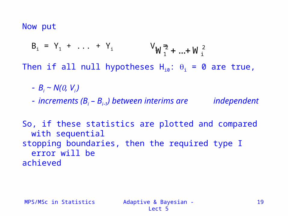
Now put
Bi = Y1 + ... + Yi Vi =
Then if all null hypotheses Hi0: i = 0 are true,
Bi ~ N(, Vi )
increments (Bi – Bi1) between interims are independent
So, if these statistics are plotted and compared with sequentialstopping boundaries, then the required type I error will beachieved
2 21 iW ... W
MPS/MSc in Statistics Adaptive & Bayesian - Lect 5 20
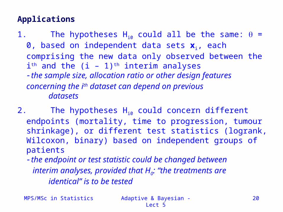
Applications
1. The hypotheses Hi0 could all be the same: = 0, based on independent data sets xi, each comprising the new data only observed between the ith and the (i – 1)th interim analyses
the sample size, allocation ratio or other design features concerning the ith dataset can depend on previous
datasets
2. The hypotheses Hi0 could concern different endpoints (mortality, time to progression, tumour shrinkage), or different test statistics (logrank, Wilcoxon, binary) based on independent groups of patients
the endpoint or test statistic could be changed between interim analyses, provided that H0: “the treatments are
identical” is to be tested
MPS/MSc in Statistics Adaptive & Bayesian - Lect 5 21
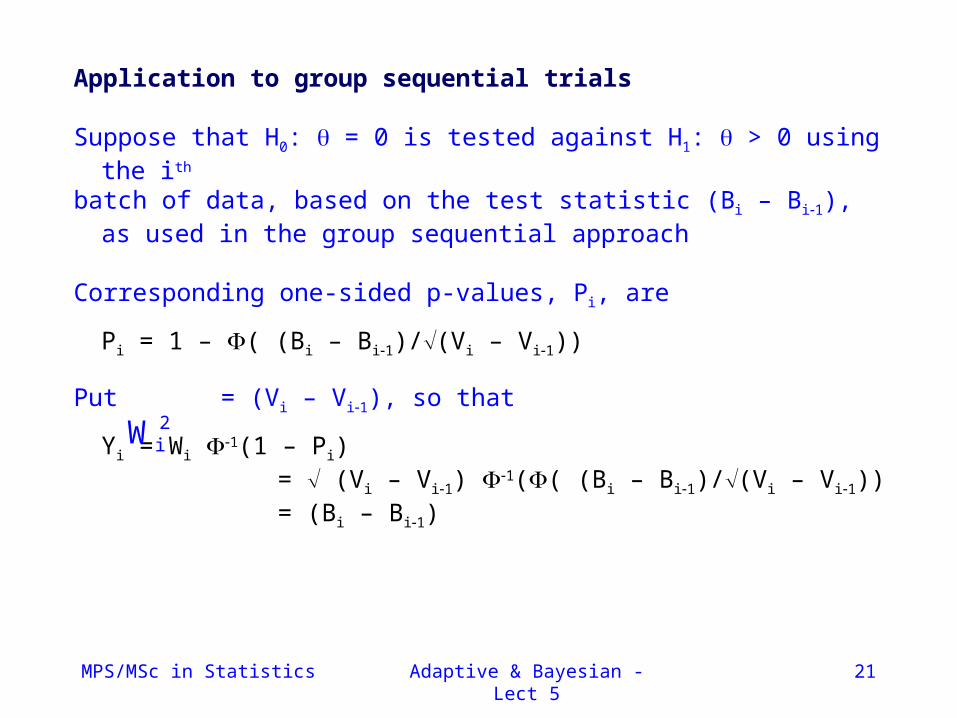
Application to group sequential trials
Suppose that H0: = 0 is tested against H1: > 0 using the ith
batch of data, based on the test statistic (Bi – Bi1), as used in the group sequential approach
Corresponding one-sided p-values, Pi, are
Pi = 1 – ( (Bi – Bi1)/(Vi – Vi1))
Put = (Vi – Vi1), so that
Yi = Wi 1(1 – Pi) = (Vi – Vi1) 1(( (Bi – Bi1)/(Vi – Vi1)) = (Bi – Bi1)
2iW
MPS/MSc in Statistics Adaptive & Bayesian - Lect 5 22
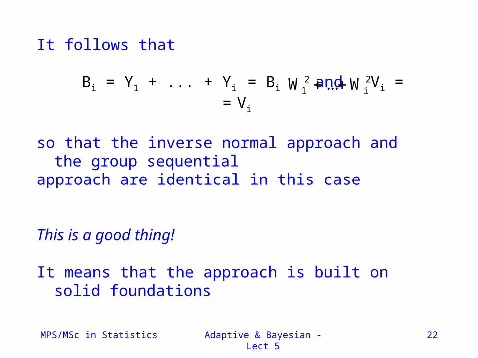
It follows that
Bi = Y1 + ... + Yi = Bi and Vi = = Vi
so that the inverse normal approach and the group sequentialapproach are identical in this case
This is a good thing!
It means that the approach is built on solid foundations
2 21 iW ... W
MPS/MSc in Statistics Adaptive & Bayesian - Lect 5 23
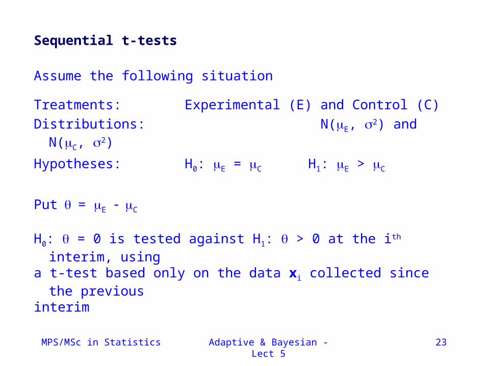
Sequential t-tests
Assume the following situation
Treatments: Experimental (E) and Control (C)
Distributions: N(E, 2) and N(C, 2)
Hypotheses: H0: E = C H1: E > C
Put= E C
H0: = 0 is tested against H1: > 0 at the ith interim, using a t-test based only on the data xi collected since the previousinterim
MPS/MSc in Statistics Adaptive & Bayesian - Lect 5 24
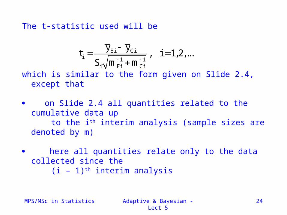
The t-statistic used will be
which is similar to the form given on Slide 2.4, except that
on Slide 2.4 all quantities related to the cumulative data up to the ith interim analysis (sample sizes are denoted by m)
here all quantities relate only to the data collected since the (i – 1)th interim analysis
Ei Cii 1 1
i Ei Ci
y yt , i 1,2,...
S m m
MPS/MSc in Statistics Adaptive & Bayesian - Lect 5 25
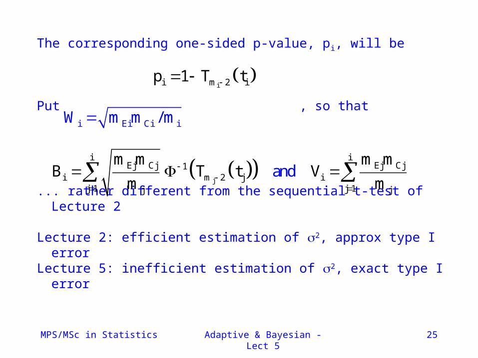
The corresponding one-sided p-value, pi, will be
Put , so that
... rather different from the sequential t-test of Lecture 2
Lecture 2: efficient estimation of 2, approx type I errorLecture 5: inefficient estimation of 2, exact type I error
ii m 2 ip 1 T t
j
i iEj Cj Ej Cj1
i m 2 j ij 1 j 1j j
m m m mB T t Vand
m m
i Ei Ci iW m m / m
MPS/MSc in Statistics Adaptive & Bayesian - Lect 5 26
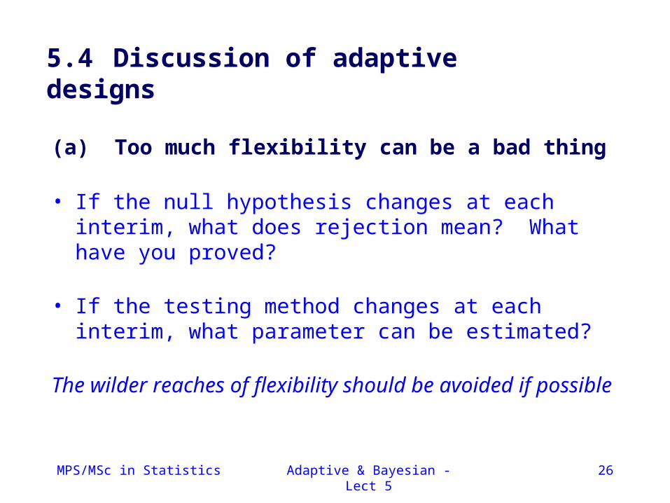
(a) Too much flexibility can be a bad thing
• If the null hypothesis changes at each interim, what does rejection mean? What have you proved?
• If the testing method changes at each interim, what parameter can be estimated?
The wilder reaches of flexibility should be avoided if possible
5.4 Discussion of adaptive designs
MPS/MSc in Statistics Adaptive & Bayesian - Lect 5 27
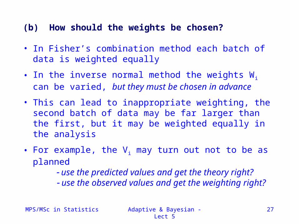
(b) How should the weights be chosen?
• In Fisher’s combination method each batch of data is weighted equally
• In the inverse normal method the weights Wi can be varied, but they must be chosen in advance
• This can lead to inappropriate weighting, the second batch of data may be far larger than the first, but it may be weighted equally in the analysis
• For example, the Vi may turn out not to be as planned use the predicted values and get the theory right?
use the observed values and get the weighting right?
MPS/MSc in Statistics Adaptive & Bayesian - Lect 5 28
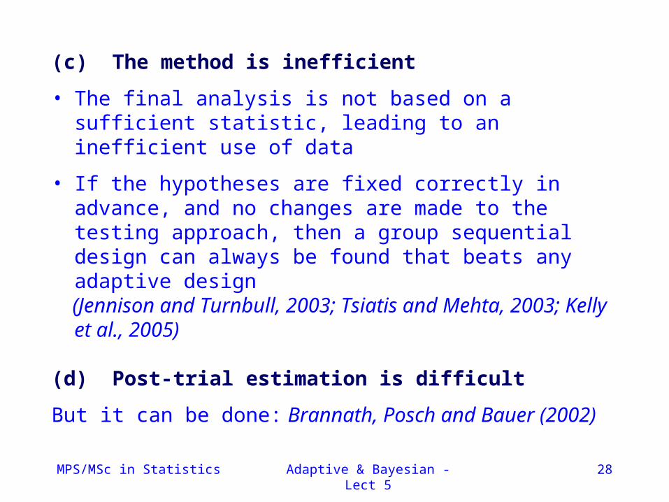
(c) The method is inefficient
• The final analysis is not based on a sufficient statistic, leading to an inefficient use of data
• If the hypotheses are fixed correctly in advance, and no changes are made to the testing approach, then a group sequential design can always be found that beats any adaptive design
(Jennison and Turnbull, 2003; Tsiatis and Mehta, 2003; Kelly et al., 2005)
(d) Post-trial estimation is difficult
But it can be done: Brannath, Posch and Bauer (2002)
MPS/MSc in Statistics Adaptive & Bayesian - Lect 5 29
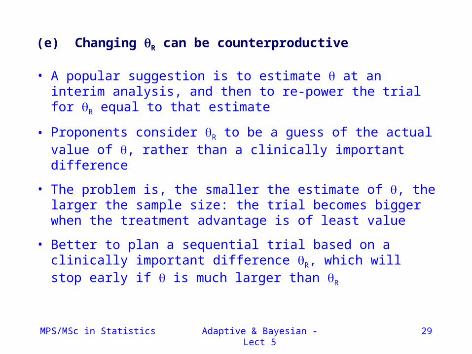
(e) Changing R can be counterproductive
• A popular suggestion is to estimate at an interim analysis, and then to re-power the trial for R equal to that estimate
• Proponents consider R to be a guess of the actual value of , rather than a clinically important difference
• The problem is, the smaller the estimate of , the larger the sample size: the trial becomes bigger when the treatment advantage is of least value
• Better to plan a sequential trial based on a clinically important difference R, which will stop early if is much larger than R