MS Excel: Analysing Data using Pivot Tables · MS Excel: Analysing Data using Pivot Tables (XL2104) 2 Because a Pivot Table report is interactive, you can change the view of the data

Centre for Learning and Academic Development (CLAD)

Technology Skills Development Team

MS Excel: Analysing Data using Pivot Tables

www.intranet.birmingham.ac.uk/itskills

http://www.intranet.birmingham.ac.uk/itskills

MS Excel: Analysing Data using Pivot Tables (XL2104)

MS Excel: Analysing Data using Pivot tables

Author: Sonia Lee Cooke (Some of the data in this course is based on a previous course

developed and presented by Barbara Hallam and Dr Graham Hendry)

Version: 1.0, October 2012

© 2009 The University of Birmingham

All rights reserved; no part of this publication may be photocopied, recorded or otherwise reproduced, stored in a retrieval system or transmitted in any form by any electrical or mechanical means without permission of the copyright holder.

Trademarks: Microsoft Windows is a registered trademark of Microsoft Corporation. All brand names and product names used in this handbook are trademarks, registered trademarks, or trade names of their respective holders.

MS Excel: Analysing Data using Pivot Tables (XL2104) i

Contents Page No.

INTRODUCTION ................................................................................................................................... 1

USING PIVOT TABLES TO ANALYSE DATA ............................................................................................. 1

WHEN TO USE A PIVOT TABLE REPORT ............................................................................................................. 1 ELEMENTS OF A PIVOT TABLE ......................................................................................................................... 2

Guidelines for creating a Pivot Table from an Excel table or data range ........................................... 4 CREATING A PIVOT TABLE ............................................................................................................................. 4 CLASSIC LAYOUT .......................................................................................................................................... 9 ADDING A CALCULATED FIELD ...................................................................................................................... 10

Removing an Error message (#DIV/0) .............................................................................................. 12 SELECTING AND FORMATTING DATA .............................................................................................................. 13 EXPAND OR COLLAPSE FIELDS IN A PIVOT TABLE .............................................................................................. 16 CHANGE THE CALCULATION IN A PIVOT TABLE ................................................................................................. 17 CHANGE CALCULATION TO PERCENTAGE ......................................................................................................... 18 REMOVE FIELDS ........................................................................................................................................ 19 ADD FIELDS TO THE PIVOT TABLE LAYOUT FORM ............................................................................................. 19

Add a Field to the Report Filter ......................................................................................................... 20 Running multiple reports from the Report Filter .............................................................................. 20 Clear the Filters ................................................................................................................................. 21

CREATING A CHART FROM A PIVOT TABLE ...................................................................................................... 21

IMPORTING DATA FROM AN ACCESS DATABASE ............................................................................... 23

EXERCISE 1 ......................................................................................................................................... 25

CREATING A PIVOT TABLE ........................................................................................................................... 25

EXERCISE 2 ......................................................................................................................................... 26

IMPORTING DATA FROM AN ACCESS DATABASE ............................................................................................... 26

MS Excel: Analysing Data using Pivot Tables (XL2104) 1

Introduction

The purpose of this course is to introduce the ideas of Pivot Tables in

Excel to those who have never used them before. Pivot tables can be

used in a fairly simple and straightforward way or be pretty complex,

depending on the data you have and what you wish to do with it. We

will confine ourselves to fairly simple examples in this course because it

is intended to raise awareness of these facilities at an introductory level.

However, I hope that it will encourage users to pursue the topics further

should they need to use them at a more sophisticated level.

The course covers some of the ways in which these facilities and tools

that are available in Excel can be used to analyse, summarise,

extrapolate from, and find solutions to problems based on information

held in Excel worksheets. Excel can also create pivot tables from

external data sources, such as Access or other ‘databases’ text files, and

sources on the Internet. You can usually specify the data you want and

retrieve the information from within the Create PivotTable dialogue

box.

The course ‘using Excel as a Database’ covers the facilities offered in

Excel for Searching, Sorting, Filtering and doing calculations on data

stored in list (or table) form in Excel worksheets. Tables in Excel are

worksheet ranges that contain information in separate columns headed

by the variable or field name with different records occupying different

rows. The table structure facilitates tasks such as sorting, filtering,

subtotalling figures, and so on.

Pivot tables take the detailed data stored in a data range or Excel table

format and help you analyse and summarise the information in an

interactive table format. The first part of this course on Pivot Tables is

in some ways a logical extension of the facilities outlined in using Excel

as a Database, which does not mean however that attendance on that

course is a pre-requisite for this course.

All the examples we are going to use for this course are in the file

XL2104 Pivot tables.xlsx.

Using Pivot Tables to analyse data

A Pivot table report is an interactive table that can be used to quickly

summarise, analyse and present large amounts of data by categories and

subcategories. You can rotate its rows and columns to see different

summaries of the source data, filter the data by displaying different

reports, or display the details for areas of interest.

When to use a Pivot Table report

You might want to use a Pivot Table report if you wish to compare

related totals, especially when you have a long list of figures to

summarise and you want to compare several facts about each figure.


Because a Pivot Table report is interactive, you can change the view of

the data to see more details or calculate different summaries.

The data area is the part of the Pivot Table report that contains summary

data. The cells of the data area show summarised data for the items in

the row and column fields. Each value in the data area represents a

summary of data from the source records or rows.

Elements of a Pivot Table

Pivot table element Definition

Row Fields Row fields are displayed on the side of the Pivot Table

report; rows can be nested within another row. A Pivot

Table report that has more than one row field has one

inner row field, the one closest to the data area; any

other row fields are referred to as outer row fields.

Inner and outer row fields have different attributes –

items in the outermost field are displayed only once,

whereas items in the rest of the fields are repeated as

necessary.

Column Field Column fields are displayed at the top of the Pivot Table

report. A Pivot Table report can have multiple column

fields just as it can have multiple row fields.

Data Item field and Summary functions

A data item field is a field from the data range or

database that contains data to be summarised. The Pivot

Table reports use summary functions such as Sum,

Count, and Average. These functions also provide

subtotals and grand totals automatically, where you

choose to show them.

By default in the data field Excel usually summarises

Row Fields

Column Fields

Data Items

Report Filter

Item Filters


numeric data by using Sum function and summarises

text data by using the Count summary function

Report Filter A Report Filter is a field that is assigned to a page or

filter orientation, it is used to filter the entire Pivot Table

report when you select an item from the drop-down list

the Pivot Table report displays the summarised data for

only that item.

Items field drop-down arrows

An item is a subcategory of a Pivot Table field. Items

represent unique entries in the same field or column in

the source data. Items appear as row or column labels

or in drop-down lists. Clicking on the drop-down arrow

at the right-hand side of each field allows you to

select the items you want to show.

Pivoting You can change the layout by dragging a field button to

another part of the Pivot Table report – e.g. move a

column to a row or a row to a column, you are

transposing the vertical or horizontal orientation of the

field (this operation is called pivoting) you can view

your data in different ways and calculate different

summarised values.

Pivot Table example

The example we are going to use is simpler and part of it is shown

below:

The table gives the numbers of pupils and staff in different types of

schools in a country district.


Using the Pivot Table function we can easily create a Pivot Table

to find out things like:

‘How many Nursery schools are there in the south west region’?

Guidelines for creating a Pivot Table from an Excel table or data range

Excel ignores any filters you have applied using commands on

the Filter submenu of the Data tab.

To create a Pivot Table from filtered data, use the Advanced

Filter command extract a range of data to another worksheet

location and base the Pivot Table on the extracted range.

Advanced filtering is covered in the ‘‘MS Excel: As a Database’

course.

Excel automatically creates grand totals and subtotals in the Pivot

Table. If the source list contains automatic grand totals, remove

them before you create the Pivot Table. Totals and subtotals

(Outlining) is also covered in the ‘MS Excel: As a Database’

course..

Because Excel uses the data in the first row of a data range or

table for the Field names in the Pivot Table, the source data

range MUST contain column headings.

To make the pivot table easier to refresh and update when the

source list or database changes, you could name the source

range and use the named range when you create the Pivot Table.

If the named range expands to include more data, you can

refresh the Pivot Table to include the new data. (If you use an

Excel Table as the data source then it will automatically have

been given a name.)

Example 1 – Number of Nursery Schools in the South-West area

Let’s say we need to analyse the data to find out, as mentioned earlier,

‘how many Nursery schools are in the south west region’, you would

create a Pivot Table.

Creating a Pivot Table

To create a Pivot Table:

Open the File you want to use (we will be using XL2104 Pivot

tablesxlsx, select the worksheet tab PivotTable).

Click on any cell in the table.


Click on the Insert tab, in the Tables group, click on the

PivotTable button to display the Create PivotTable dialogue box:

Under Choose the data that you want to analyze: Select a

table or range is the default.

The Table/Range: is already selected for you. Excel will

automatically select the data range, as long as it recognises your

data range or table (which it should do if you have obeyed the

rules, see page 4, Guidelines for creating a Pivot Table from

an Excel table or data range).

Under Choose where you want the PivotTable report to be

placed: are two options: you can insert the Pivot Table in a New

worksheet or Existing worksheet (the same worksheet as your

table or data range). For simplicity in this course (so we don’t

end up with dozens of worksheets) we will put our Pivot Table on

the same worksheet. This also has the advantage that we can

see them all and compares the results we get.

Select Existing worksheet, then click in the Location text box

and click on cell H5 in the current worksheet to specify where

you want to start the Pivot Table.

Click on the OK button. This brings you back to the worksheet

which now has a blank Pivot Table and PivotTable Field List as

shown below:


At the same time, two additional, contextual tabs appear on the Ribbon under the heading PivotTable Tools. There is an Options tab, which should be selected, and a Design to change the appearance of the pivot table.

The field names in our original data range are shown in the floating PivotTable Field List dialogue box.

Let’s say we want to know ‘how many Nursery schools are in

the south west area’. Under Choose fields to add to report:

Drag the required field – e.g. ‘Area’ from the list into the Column Labels box. The column labels will be added to the pivot table.

Drag the field ‘Type’ into the Row Labels box. Your pivot table and field list should now look something like this.

Empty Pivot Table because no fields have been selected yet

Click on this button and select a style from the drop-down list to change the layout of the PivotTable Field List dialogue box

Drag fields into these drop boxes to build a table

Field names from the data range


The pivot table, by default, is created using the Compact Layout. At this point, it is helpful to switch to Outline Layout, which shows the names of the fields, instead of just saying Row Labels and Column Labels.

Select the PivotTable Tools Design tab in the Ribbon.

In the Layout group, click on Report Layout, and choose Show

in Outline Layout. Your pivot table should now look like this:

Drag the field ‘Name’ into the Values box. Name is the appropriate field to use if we want to know the number of schools in the South-West area. Excel will automatically use the Count summary function.

The Pivot Table produced should look like this, and the top left cell will be in H5 as requested.

If you click outside of the Pivot Table, the PivotTable changes

its appearance and the PivotTable Field List disappears, click


on the Pivot Table again and the PivotTable Field List appears

and so do the two PivotTable Tools tabs on the Ribbon.

If the PivotTable Field List dialogue box does not appear, switch

to the Pivot Table Tools Options tab on the Ribbon and ensure

that the Field List button in the Show/Hide group is selected.

The drop-down arrows next to Type and Area (shown below)

produce the following lists of selection boxes:

If you want to see just the Nursery schools in the south west

(SW) area, deselect the other options and the Pivot Table then

looks like this:

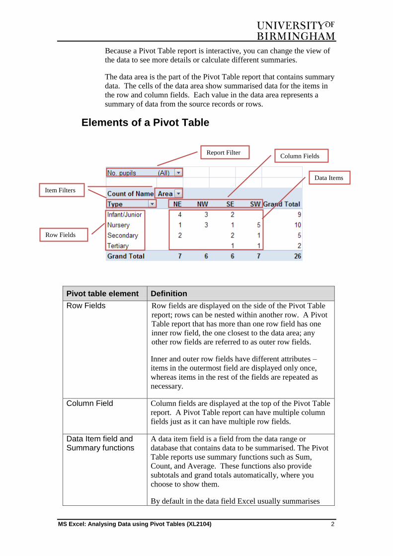
Excel automatically displays Subtotals and Grand Totals; you

can show or hide the Grand Totals by clicking on the Options

tab and in the Pivot Table group select Options to open the

PivotTable Options dialogue box.


Click on the Totals & Filters tab and under Grand Totals; deselect Show grand totals for rows or Show grand totals for columns and click OK. Alternatively, click on the Design tab, in

the Layout group, click on Grand Totals and select the appropriate option.

Classic Layout

Using the Classic layout

If you've used pivot tables in an earlier version of Excel, you may

be used to the older form based layout, which lets you drag fields

directly onto the table. You can switch to this layout using the

PivotTable Options dialogue box.

Open the PivotTable Options dialogue box as above, and switch

to the Display tab.

Tick the box labelled Classic PivotTable layout (enables

dragging of fields into the grid).


Your pivot table changes to look like this:

You can now drag fields directly onto the different areas of the

table.

Adding a Calculated Field

Example 2. How many pupils and staff in schools for each area and the pupil/staff ratio:

Click back in the original data range and then on the Insert tab

and in the Table group, click on PivotTable, the Create

PivotTable dialogue box appears.

Select the Location for the Pivot Table – e.g. cell H18 and click

OK.

Drag the appropriate Fields from the PivotTable Field List to the

required box:

Drag Type to the Row Labels box

Drag Area to the Column Labels box

Drag No. pupils to the Values box

Drag No. staff to the Values box.

This will create a new field called Σ Values - drag this to the Row

Labels box.

Select the PivotTable Tools Design tab on the Ribbon. In the Layout group, click on Report Layout and choose Show in Outline Layout.


The following Pivot Table will be produced:

To get the pupils/staff ratio, click on the Options tab and in the

Calculations group

Click on the Fields, Items, & Sets button then select Calculated Field…

The Insert Calculated Field dialogue box appears:

In the Name: box type ‘Pupils Staff Ratio’

In the Formula: text box delete the zero.

Under Fields: select ‘No. pupils’ and click on the Insert Field

button at the bottom of the list. Type in a forward slash ‘/’. Select

‘No. staff’ and click on the Insert Field button again.

Alternatively, double-click on the field name.

Click on the Add button.

Click OK, to insert the Pupils Staff Ratio field as show below:


The Pivot Table will now look something like this:

Excel introduces the new calculation as Sum of Pupils Staff

Ratio which of course it isn’t; this is just Excel speak! Excel has

taken the total number of pupils and the total number of staff in a

given category, or overall, and divided one by the other in each

case.

Removing an Error message (#DIV/0)

The #DIV/0! Errors - To get rid of the divide by zero errors:

Click on the Pivot Table to make it active.


Click on the Options tab and in the Pivot Table group, click on

Options and select Options, the PivotTable Options dialogue box appears:

Under Format, click in the box For error values show: and type,

a value you want to appear in your Pivot Table to replace the

division error, for example, two hyphens (--). Excel will interpret

one hyphen as a minus, so choose something appropriate.

Click OK.

Selecting and formatting data

To select data in a Pivot Table:

Point the mouse to the cell containing the data you want to select

– e.g. we are going to select Sum Pupils Staff ratio

Point the mouse to the left of the field (Sum of Pupils Staff

ratio) until the mouse pointer change to a black horizontal

arrow (as shown below)


Click once on the Field to highlight the labels and the cells

containing the data ‘Sum of Pupil Staff ratio’ currently

expressed to many places of decimals.

To select the cells that contains just the values, click on the Options tab, in the Actions group, click on Select and choose Values.


To format the Pivot Table:

Click on the Options tab and in the Active Field group; click on Field Setting, the Value Field Settings dialogue box appears

Click on the Number Format button, The Format Number

dialogue box appears, select Number from the list and change

the Decimal places: to 1

Click OK twice to return to the worksheet, notice that the

worksheet column widths are automatically formatted. The Pivot

Table should look like this:


Alternatively, you can right click on one of the cells highlighted,

choose Number Format… from the short-cut menu and format

the number to say one decimal place (as before).

You could also make these cells bold so that they stand out from

the rest.

Expand or Collapse fields in a Pivot Table

To expand or collapse a field:

Select the field you want to Expand or Collapse. In this case

right-click on Secondary, under the Type field column. From the

context menu choose Expand/Collapse and then Expand

This will open up a dialogue box where you can choose what field

you want to show in the expanded view. In this case, choose

Name.

To hide the details for the entire field, click on the Options tab, in the Active Field group; click on the Collapse Entire Field button

Excel will automatically collapse all fields.


If you click the Expand Entire Field button Excel will automatically expand all fields.

All the Secondary schools will now be listed by name and the

middle part of your Pivot Table will now look something like this:

Tip

If you want to look at the detail behind the figure of 17.5 as the Grand Total

for Sum of Pupils Staff Ratio for Secondary schools, you can double

click on that cell and Excel will produce the following table on a new

worksheet which it automatically inserts to the left of the current active

worksheet.

Change the calculation in a Pivot Table

By default Excel uses Sum function for numeric data and Count function for non-numeric data:

To change the calculation in a Pivot Table data field – e.g. let’s say you want Average instead of Sum.

Click on the field you want to change in the Pivot Table, say ‘Sum of No. Pupils’


Click on the Options tab and in the Active Field group, click on

Field Settings the Value Field Settings dialogue box appears:

Click on the Summarize value field by tab and select Average from the list.

Alternatively, right-click on the field ‘Sum of No. Pupils’ and select Value Field Settings… from the drop-down menu, or double-click on the field.

Click the OK button to change the Sum function to Average.

Change calculation to percentage

If you want to express your calculations as percentages or differences:

Click on the Options tab and in the Active Field group, click on Field Settings, the Value Field Settings dialogue box appears:


Click on the Show values as tab, under then click on the arrowhead to the right of Normal and select an option from the list.

Click on the OK button.

Remove Fields

To remove a field from the Pivot Table:

Click on the Field you want to remove and drag it away from the boxes at the bottom of the PivotTable Field List, the Mouse Pointer will change to a cross, release the mouse button and drop the field on the worksheet to remove the field.

Alternatively, right-click on the field and select Remove from the

list.

Add Fields to the Pivot table Layout Form

To add a Field to the Pivot Table:

Drag the field from under Choose fields to add to report: and drop it into the relevant text box under Drag fields between areas below:


If you simply tick the checkbox for a field without dragging it, the field is placed in a default area on the Pivot Table – i.e. non-numeric fields are added to the row area and numeric fields are added to the data item area.

Add a Field to the Report Filter

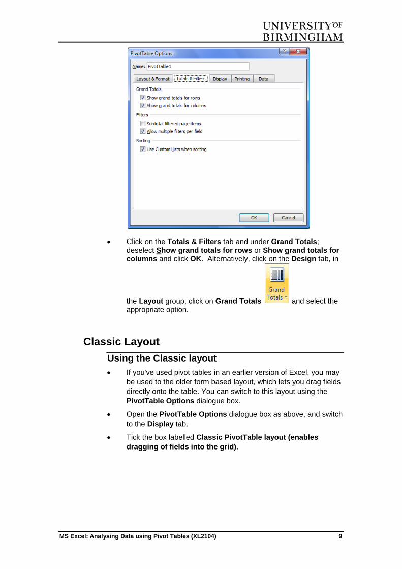
A Report Filter at the top of the Pivot Table allows you to display only one item or all items:

Simply drag the field from the PivotTable Field List and drop it

into the Report Filter box. The filter will appear above the pivot

table:

Click on the arrowhead and select the Item you want to display.

Running multiple reports from the Report Filter

If you want to run a report on all of the items listed in the drop-down menu on the Report Filter.

Click on the Options tab and in the Pivot Table group, click on Options, and then click on Show Report Filter Pages…


The Show Report Filter Pages dialogue box appears:

Click on the Ok button

Excel generates a summary report of all the items listed in the

Page Field on separate worksheet.

Clear the Filters

To clear the filters:

Click on the Options tab and in the Actions group, click on Clear and select one of the following options: clear all filters or clear filters.

Creating a Chart from a Pivot Table

To create a chart of the information shown in the Pivot Table:

Click in the Pivot Table

Removes all fields formatting and

filters and displays the blank Pivot

Table Layout form

Clears all current filters


Click on the Options tab and in the Tools group, click on

PivotChart

The Insert Chart dialogue box appears:

Select the chart you want and click OK, Excel will produce a chart together with the PivotChart Filter Pane, the chart may not be as you want it.

Click on the Layout tab to format the chart or the Design tab to

change the chart styles.


Importing Data from an Access Database

One of the limitations of using Pivot Tables in Excel is simply the

number of rows in an Excel worksheet. For many this is not a practical

problem, particularly since the old limit of 65,536 rows has been

increased to over a million in Excel 2010. However, you may wish to

analyse a dataset that contains more than this number of records.

An Access table can hold many millions of records. In fact the only

limit to number of records in Access is that a database file cannot

exceed 2 Gigabytes in size.

Remarkably, Excel can link to an Access table (or query) of any size,

and then pivot the results. This is phenomenally useful.

The pivoting process is identical to the one you have already explored.

The only difference is how you connect to an Access database.

To get the Access database:

Open Microsoft Excel (if it’s not already open)

Click on the Insert tab in the Tables group, click on Pivot Table the Create PivotTable dialogue box appears:

Select Use an external data source and click on the Choose

Connection… button to display the Existing Connections

dialogue box, click on the Browse for more… button at the

bottom left.

The Select Data Source dialogue box appears, locate the access file you want to import.


The Select Table dialogue box appears

Select the table you want to export to Excel. We are going to use tbl_Employees.

Click on the Ok button, which takes you back to the Create PivotTable dialogue box

Choose where you want the Pivot Table report to be placed – e.g. New Worksheet.

Click on the Ok button.

Excel generates a blank Pivot Table and the PivotTable Field List dialogue box.

Drag the required fields from under Choose fields to add to report: to the relevant text boxes below Drag fields between areas below:


Exercise 1

Creating a Pivot Table

Please complete the exercise below:

Create a Pivot Table showing the Average number of Pupils in

the different types of schools in the four geographical areas; i.e.

average number of pupils in Infant Junior in NE, NW, SE and

SW. Insert the Pivot Table in your current worksheet.

Format the values to be whole numbers.

Change the labels to show the field names – (Type and Area)

instead of Row Labels and Column Labels

Note

If you need help to show the Average Number of Pupils, take a look at

page 17 – Change the calculation in a Pivot Table in your User Guide.

(MS Excel: Analysing Data using Pivot Tables)

Your Pivot Table should look like this:


Exercise 2

Importing Data from an Access database

You might like to try this now using information in a table in one of the

databases used in Access Courses.

Please complete the following exercise:

Insert a new worksheet and name it Sales Dept.

We are going to import Emp database, which is stored in

C:\Docs\Access.

Create a Pivot Table report, to show the salary of all the people

in the Sales Department.

Change the labels to show the field names – (Lastname and

Sales) instead of Row Labels and Column Labels.

Remove the Grand Total Row from the Pivot Table.

Note

The best orientation is probably to have Department going across the top as

columns and Last Name as rows.

If you need help take a look at page 23 (Importing Data from an Access

Database) in your User Guide (MS Excel: Analysing Data using Pivot

Tables)

Your Pivot Table should look like this:

Documents

MS Excel: Analysing Data using Pivot Tables · MS Excel: Analysing Data using Pivot Tables (XL2104) 2 Because a Pivot Table report is interactive, you can change the view of the data