MSAFC: matrix subspace analysis with fuzzy clustering ability

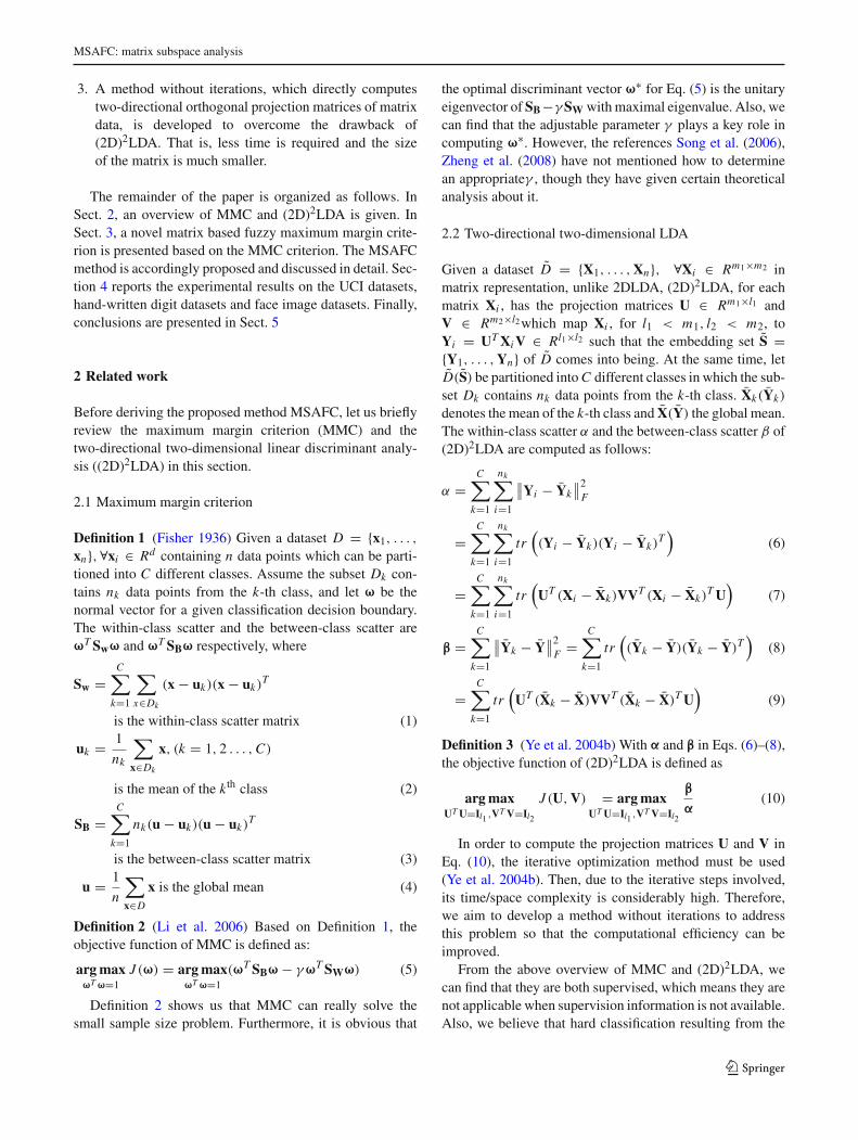
Soft ComputDOI 10.1007/s00500-013-1134-3

METHODOLOGIES AND APPLICATION

MSAFC: matrix subspace analysis with fuzzy clustering ability

Jun Gao · Fulai Chung · Shitong Wang

© Springer-Verlag Berlin Heidelberg 2013

Abstract In this paper, based on the maximum margin cri-terion (MMC) together with the fuzzy clustering and thetensor theory, a novel matrix based fuzzy maximum mar-gin criterion (MFMMC) is proposed and based upon whicha matrix subspace analysis method with fuzzy clustering abil-ity (MSAFC) is derived. Besides, according to the intuitivegeometry, a proper method of setting the adjustable parame-ter γ in the proposed criterion MFMMC is given and its ratio-nale is provided. The proposed method MSAFC can simul-taneously realize unsupervised feature extraction and fuzzyclustering for matrix data (e.g. image data). As to the runningefficiency of MSAFC, a two-directional orthogonal methodof dealing with matrix data without any iteration is developedto improve it. Experimental results on UCI datasets, hand-written digit datasets, face image datasets and gene datasetsshow the distinctive performance of MSAFC.

Keywords Matrix subspace analysis · Two-directional 2Dfeature extraction · Matrix based fuzzy maximum margincriterion · Fuzzy clustering

Communicated by W. Pedrycz.

J. GaoSchool of Information Engineering, Yancheng Instituteof Technology, Yancheng, Jiangsu, China

J. Gao · S. WangSchool of Digital Media, Jiangnan University,Wuxi, Jiangsu, China

F. Chung · S. Wang (B)Department of Computing, Hong Kong Polytechnic University,Hong Kong, Chinae-mail: [email protected]

1 Introduction

Various feature extraction techniques for preprocessing datahave been developed and successfully used in the fields ofpattern recognition, image processing and computer vision(Turk and Pentland 1991; Cui and Gao 2005; Fu et al. 2007;Ye and Liu 2009). They aim at transforming a source highdimensional sample space into a low dimensional represen-tative space (Bian and Zhang 2001) through feature transfor-mation mapping. The efficiency of them depends on the dis-criminative information left in the corresponding low dimen-sional representative space. Hence, two traditional featureextraction methods, i.e. principal component analysis (PCA)(Jolliffe 1986; Choi and Park 2009) and linear discriminationanalysis (LDA) (Fisher 1936; Hsieh et al. 2006; Kim et al.1998), have drawn much attention of researchers in the pastdecades. As an unsupervised method, PCA helps to select theprincipal components (namely, a group of mutually orthogo-nal axes) that can keep the global information of the samplesthrough constructing a covariance matrix, thus getting thelow dimensional projection of the source sample space fromthese principal components. LDA, as a supervised featureextraction method, makes full use of the class labels of train-ing samples and realizes its low dimensional embedding ofthe source high dimensional space according to the princi-ple of minimum within-class scatter and maximum between-class scatter. Hence, LDA is obvious better than PCA inidentifying the hidden structures and features of differentclasses when the class labels of training samples are available(Fisher 1936; Hsieh et al. 2006; Kim et al. 1998; Martínezet al. 2001). Though, when LDA is applied to a small-sizedataset having high-dimensional features, the correspondingwithin-class scatter is likely to be singular, which is called asthe Small Sample Size (SSS) problem. This problem makesLDA unable to get the optimal discriminative vector to a

123

J. Gao et al.

certain extent. In order to overcome this drawback, variantsof LDA have been proposed from different aspects, includingPCA+LDA (Wang and Tang 2004), Fisherface method (Fuet al. 2007; Ye and Liu 2009), Discriminant Learning Analy-sis (DLA) (Peng et al. 2008). Among them, we focus on themaximum distance based methods using Maximum ScatterDifference (MSD) discriminative criterion (Song et al. 2006),Maximum Margin Criterion (MMC) (Li et al. 2006) and Reg-ularized MMC (RMMC) (Zheng et al. 2008). They indeedcan avoid the SSS problem occurring in LDA by computingthe difference between the maximum between-class scatterand the minimum within-class scatter instead of computingtheir ratio as in LDA. Moreover, they usually have compar-atively lower time complexity than other existing methods(Liu et al. 2007).

Currently, more and more data in the field of intelligentrecognition can be represented as tensor data (Yan et al. 2007;Daizhan et al. 2013), such as matrix face images (second-order tensors) (Yan et al. 2007; Lei et al. 2007), color images(third-order tensors) (Kim and Choi 2007), colorful videosignals (fourth-order tensors) (Lu et al. 2009) and so on.When the traditional subspace learning methods are usedto vectorize these high dimensional tensor data, the curseof dimensionality may occur (Ren and Dai 2010) and theintrinsic geometric structure and the correlation of sourcedata may also be destroyed. Therefore, tensor based subspacelearning methods have been developed in depth to overcomethese difficulties in recent years. Most of them are rootedat PCA or LDA. For example, PCA based two-dimensionalPCA (2DPCA) (Yang et al. 2004) realizes low dimensionalembedding along with only the row direction for matrix pat-terns by constructing a covariance matrix. Two-directionaltwo-dimensional PCA ((2D)2PCA) (Zhang and Zhou 2005),generalized low rank approximations of matrices (GLRAM)(Ye 2005) and generalized PCA (GPCA) (Ye et al. 2004a)can realize two-directional feature extraction in matrix mode.In (Lu et al. 2008), GPCA is generalized into multilinearPCA (MPCA) for high-order tensor patterns. In (Lu et al.2009, 2011), as an improved version of MPCA, uncorre-lated multilinear PCA (UMPCA) has been developed to real-ize uncorrelated feature extraction by using zero-correlationconstraints for high-order tensor patterns. Similarly, based onLDA, two-dimensional LDA (2DLDA) (Li and Yuan 2005;Xiong et al. 2005; Jing et al. 2006) was proposed. It can-not only effectively reduce the time and space complexitiesfor computing the between-class scatter and the within-classscatter in LDA, but also overcome the SSS problems (at leastto a certain extent) in LDA, thus improving its robustness andgeneralization capability. Furthermore, two-directional two-dimensional LDA ((2D)2LDA)1 was developed to simulta-

1 Although it is also called as 2D-FLD, it is a two-direction two-dimensional feature extraction method in nature. In order to distinguish

neously consider the discriminative information in both therow and the column directions of matrix data. In (Yan et al.2007), (2D)2LDA was extended into its generalized versionDATER for high order tensor data. In (Wang et al. 2008)the tensor theory is introduced into the MSD method and thetwo-dimensional MSD (2DMSD) method is accordingly pro-posed to overcome the drawback: the discriminative informa-tion in the column direction of matrix data is not consideredfully when 2DMSD extracts features. In (Tao et al. 2007),based on 2DMSD+PCA,the general discriminant analysis(GTDA) is proposed.

It has drawn our attention that in (Gao and Wang 2009; Liet al. 2011; Yang et al. 2008, 2010), the fuzzy theory has beenintegrated into feature extraction from different aspects. Inparticular, on the basis of MMC and LDA respectively, twounsupervised feature extraction methods, FMSDC (MSD-based fuzzy clustering) (Gao and Wang 2009) and FLDC(LDA-based fuzzy clustering) (Li et al. 2011), have beenproposed to simultaneously realize fuzzy clustering and fea-ture extraction by introducing memberships into the corre-sponding within-class and between-class scatters. In (Yanget al. 2008, 2010), the fuzzy concept are introduced intoLDA and 2DLDA respectively such that CFLDA (completefuzzy LDA) and F2DLDA (fuzzy 2DLDA) are developed toimprove the generalization power of LDA.

As we know, (2D)2PCA, (2D)2LDA and 2DMSD+PCAcannot directly realize clustering for matrix data and FMSDCand FLDC can only deal with low dimensional data. As forCFLDA and F2DLDA, although they have considered thefuzzy concept, they cannot be used to cluster data directlybecause they both use priori estimation methods when com-puting the corresponding memberships. So, in order toachieve both feature extraction and clustering of matrix data,in this paper we propose a matrix based fuzzy maximum mar-gin criterion (MFMMC) which combines the advantages ofthe state-of-the-art methods with MMC and then constructa novel matrix subspace discriminant analysis method withfuzzy clustering ability (MSAFC). Herein, we only considersecond-order tensor (i.e. matrix patterns) data for simplicity.Three main contributions of our work can be highlighted asfollows:

1. In contrast to (2D)2LDA, MSAFC based on the pro-posed matrix based fuzzy maximum margin criterion cansimultaneously realize fuzzy clustering for matrix dataand two-directional two-dimensional unsupervised fea-ture extraction.

2. Based on the intuitive geometry and theoretical analysis,an appropriate technique of setting the adjustable para-meter γ in the proposed criterion MFMMC is given.

Footnote contiuned 1it from other single-direction two-dimensional feature extraction meth-ods, we take it as (2D)2LDA in this paper.

123

MSAFC: matrix subspace analysis

3. A method without iterations, which directly computestwo-directional orthogonal projection matrices of matrixdata, is developed to overcome the drawback of(2D)2LDA. That is, less time is required and the sizeof the matrix is much smaller.

The remainder of the paper is organized as follows. InSect. 2, an overview of MMC and (2D)2LDA is given. InSect. 3, a novel matrix based fuzzy maximum margin crite-rion is presented based on the MMC criterion. The MSAFCmethod is accordingly proposed and discussed in detail. Sec-tion 4 reports the experimental results on the UCI datasets,hand-written digit datasets and face image datasets. Finally,conclusions are presented in Sect. 5

2 Related work

Before deriving the proposed method MSAFC, let us brieflyreview the maximum margin criterion (MMC) and thetwo-directional two-dimensional linear discriminant analy-sis ((2D)2LDA) in this section.

2.1 Maximum margin criterion

Definition 1 (Fisher 1936) Given a dataset D = {x1, . . . ,

xn},∀xi ∈ Rd containing n data points which can be parti-tioned into C different classes. Assume the subset Dk con-tains nk data points from the k-th class, and let ω be thenormal vector for a given classification decision boundary.The within-class scatter and the between-class scatter areωT Swω and ωT SBω respectively, where

Sw =C∑

k=1

∑

x∈Dk

(x − uk)(x − uk)T

is the within-class scatter matrix (1)

uk = 1

nk

∑

x∈Dk

x, (k = 1, 2 . . . , C)

is the mean of the kth class (2)

SB =C∑

k=1

nk(u − uk)(u − uk)T

is the between-class scatter matrix (3)

u = 1

n

∑

x∈D

x is the global mean (4)

Definition 2 (Li et al. 2006) Based on Definition 1, theobjective function of MMC is defined as:

arg maxωT ω=1

J (ω) = arg maxωT ω=1

(ωT SBω − γωT SWω) (5)

Definition 2 shows us that MMC can really solve thesmall sample size problem. Furthermore, it is obvious that

the optimal discriminant vector ω∗ for Eq. (5) is the unitaryeigenvector of SB −γ SW with maximal eigenvalue. Also, wecan find that the adjustable parameter γ plays a key role incomputing ω∗. However, the references Song et al. (2006),Zheng et al. (2008) have not mentioned how to determinean appropriateγ , though they have given certain theoreticalanalysis about it.

2.2 Two-directional two-dimensional LDA

Given a dataset D = {X1, . . . , Xn}, ∀Xi ∈ Rm1×m2 inmatrix representation, unlike 2DLDA, (2D)2LDA, for eachmatrix Xi , has the projection matrices U ∈ Rm1×l1 andV ∈ Rm2×l2 which map Xi , for l1 < m1, l2 < m2, toYi = UT Xi V ∈ Rl1×l2 such that the embedding set S ={Y1, . . . , Yn} of D comes into being. At the same time, letD(S) be partitioned into C different classes in which the sub-set Dk contains nk data points from the k-th class. Xk(Yk)

denotes the mean of the k-th class and X(Y) the global mean.The within-class scatter α and the between-class scatter β of(2D)2LDA are computed as follows:

α =C∑

k=1

nk∑

i=1

∥∥Yi − Yk∥∥2

F

=C∑

k=1

nk∑

i=1

tr((Yi − Yk)(Yi − Yk)

T)

(6)

=C∑

k=1

nk∑

i=1

tr(

UT (Xi − Xk)VVT (Xi − Xk)T U

)(7)

β =C∑

k=1

∥∥Yk − Y∥∥2

F =C∑

k=1

tr((Yk − Y)(Yk − Y)T

)(8)

=C∑

k=1

tr(

UT (Xk − X)VVT (Xk − X)T U)

(9)

Definition 3 (Ye et al. 2004b) With α and β in Eqs. (6)–(8),the objective function of (2D)2LDA is defined as

arg maxUT U=Il1 ,VT V=Il2

J (U, V) = arg maxUT U=Il1 ,VT V=Il2

β

α(10)

In order to compute the projection matrices U and V inEq. (10), the iterative optimization method must be used(Ye et al. 2004b). Then, due to the iterative steps involved,its time/space complexity is considerably high. Therefore,we aim to develop a method without iterations to addressthis problem so that the computational efficiency can beimproved.

From the above overview of MMC and (2D)2LDA, wecan find that they are both supervised, which means they arenot applicable when supervision information is not available.Also, we believe that hard classification resulting from the

123

J. Gao et al.

above two methods is not always rational and fuzzy clas-sification may sometimes be more suitable for many sce-narios in the real world. Hence, in the following section, amatrix based fuzzy maximum margin criterion (MFMMC)is proposed by integrating the fuzzy concept and the tensortheory into MMC. And based upon this criterion, a novelmethod MSAFC for matrix data is derived. The proposedmethod can realize both clustering and unsupervised fea-ture extracting for matrix data. At the same time, we pro-pose a method to properly set the adjustable parameter γ

in MFMMC from the intuitively geometrical and theoreti-cal perspectives. We also develop a method to effectivelycompute the two projection matrices U and V such thatthe corresponding computing efficiency can be significantlyenhanced.

3 Matrix subspace analysis with fuzzy clustering ability

Most of the existing features extraction methods for matrixdata cannot be used to extract features and achieve cluster-ing/classification at the same time. When applying them toclustering/classification tasks for matrix data, one need tofirst extract important features from matrix data, and thenuse a popular clustering/classification method to completethe required clustering/classification tasks. Typical exam-ples include the no-negative multilinear PCA (NMPCA) inPanagakis et al. (2010) and the tensor-based EEG classifica-tion(TEEG) in Li et al. (2009). In NMPCA, k-NN or SVM areadopted for classification after feature extraction. In TEEGgeneral discriminant analysis (GTDA) (Tao et al. 2007) isadopted for feature extraction but VM is adopted for clas-sification. As far as we know, no attention has been paid tohow to realize joint feature extraction and fuzzy clusteringfor unsupervised matrix data.

Although it seems that we can easily fuzzify matrix basedfeature extraction methods using methods similar to those inFMSDC (Gao and Wang 2009) and FLDC (Li et al. 2011),we can still obtain new observations from this study, includ-ing the appropriate choice of certain adjustable parametersand the efficient computation on two-directional orthogo-nal projection matrices of matrix data. So it is worthwhileto study how to simultaneously realize feature extractionand fuzzy clustering for matrix data. In this section, wewill propose one such method called MSAFC based onthe proposed matrix based fuzzy maximum margin criterionMFMMC.

3.1 Matrix based fuzzy maximum margin criterion

MFMMC is actually an unsupervised feature extraction cri-terion, and its within-class and between-class scatters thereinare different from LDA and MMC in the sense of its math-

ematics. Hence, we need to redefine the within-class scatterαMFMMC and the between-class scatter βMFMMC in MFMMC.

Definition 4 D = {X1, . . . , Xn} ⊆ Rm1×m2 is a matrixdataset in which the data points can be partitioned into Cclasses. For ∀Xi , there exist two projection matrices U ∈Rm1×l1 and V ∈ Rm2×l2 at the same time such that Xi ismapped into Yi = UT Xi V ∈ Rl1×l2 , l1 < m1, l2 < m2. Weget the embedding set S of D, i.e., S = {Y1, . . . , Yn}. So thewithin-class scatter αMFMMC and the between-class scatterβMFMMC can be written respectively as follows:

αMFMMC =C∑

k=1

n∑

i=1

μmik

∥∥Yi − Yk∥∥2

F

=C∑

k=1

n∑

i=1

μmik tr

((Yi − Yk)(Yi − Yk)

T)

(11)

=C∑

k=1

n∑

i=1

μmik tr

(UT (Xi −Xk)VVT (Xi −Xk)

T U)

(12)

=C∑

k=1

n∑

i=1

μmik tr

(VT (Xi −Xk)

T UUT (Xi −Xk)V)

(13)

βMFMMC =C∑

k=1

n∑

i=1

μmik

∥∥Yk − Y∥∥2

F (14)

=C∑

k=1

n∑

i=1

μmik tr

((Yk − Y)(Yk − Y)T

)

=C∑

k=1

n∑

i=1

μmik tr

(UT (Xk − X)VVT (Xk − X)T U

)

(15)

=C∑

k=1

n∑

i=1

μmik tr

(VT (Xk − X)T UUT (Xk − X)V

)

(16)

where μik denotes the membership which represents whatdegree the i-th sample belong to the k-th class with∑C

k=1 μik = 1, m is the fuzzy index with m > 1, Xk (orYk) denotes the fuzzy clustering center of the k-th class in D(or S) and X (or Y) is the global mean of D (or S), namely,X = 1

n

∑Xi ∈D Xi (or Y = 1

n

∑Yi ∈S Yi ).

Definition 5 Based on Eqs. (11)–(15) in Definition 4, wehave the following objective function of MFMMC:

arg maxUT U=Il1 ,VT V=Il2 ,�,�

J (U, V) = arg maxUT U=Il1 ,VT V=Il2 ,�,�

βMFMMC

−γαMFMMC (17)

where � = (μi j )n×C is a n × C membership matrix, γ is apositive adjustable parameter and � = {X1, . . . , XC }.

123


Definitions 4 and 5 above show us that the obvious differ-ences between the within-class and between-class scatters ofMFMMC and those of (2D)2LDA exist in: (1) the scatters inMFMMC are fuzzified; (2) Xk(orYk) in MFMMC denotesthe fuzzy clustering center of the k-th class in D(orS) insteadof the mean of the k-th class and is computed on the basisof the unsupervised method instead of the supervised one;(3) the membership μik obtained through optimization candirectly provide us the corresponding unsupervised classifi-cation.

Theorem 1 In MFMMC, necessary conditions of Eq. (17)are

μik =(∥∥Yi − Yk

∥∥2F − 1

γ

∥∥Yk − Y∥∥2

F

)(1/1−m)

∑Cj=1

(∥∥Yi − Y j∥∥2

F − 1γ

∥∥Y j − Y∥∥2

F

)(1/1−m)(18)

=(

tr(UT (Xi −Xk)VVT (Xi −Xk)

T U)− 1

γtr

(UT (Xk −X)VVT (Xk −X)T U

))(1/1−m)

∑Cj=1

(tr

(UT (Xi −X j )VVT (Xi −X j )T U

)− 1γ

tr(UT (X j −X)VVT (X j −X)T U))(1/1−m)

(19)

and

Yk =∑n

i=1 μmik

(Yi − 1

γY

)

∑ni=1 μm

ik

(1 − 1

γ

) . (20)

Proof We first prove Eqs. (18) and (19).

According to the Lagrange multiplier method, the corre-sponding Lagrange function of Eq. (17) is as follows:

L = J (U, V) − η1(UT U − Il1) − η2(VT V − Il2)

+C∑

k=1

λi (μik − 1) (21)

where η1, η2, λi are Lagrange coefficients.In order to make Eq. (17) valid, we should set

∂L

∂μik= 0

i.e. μik =(

λi

m(γ ‖Yi − Yk‖2F − ‖Yk − Y‖2

F )

) 1m−1

(22)

Since∑C

j=1 μi j = 1,

we have λ1/(m−1)i = 1

∑Cj=1(γ ‖Yi −Y j‖2

F −‖Y j −Y‖2F )1/(1−m)

(23)

Substituting Eq. (22) into Eq. (23), we can see that Eq.(18) holds. Substituting Eqs. (12) and (15) into Eq. (18), wecan also see that Eq. (19) holds.

Using the same trick, we can easily prove Eq. (20). Thus,this theorem holds. ��

We should note that Eqs. (18) and (19) do not alwayssatisfy μik ∈ [0, 1]. Therefore, we can set μik = 1, μi j =0, k = j when

‖Yi − Yk‖2F ≤ 1

γ‖Yk − Y‖2

F (24)

i.e.

tr(


)

≤ 1

γtr


). (25)

The above specification comes from our intuition, i.e., ∀Xi ,the distance between its projection and the projection of theclustering center of the k-th class is less than or equal to 1/

√γ

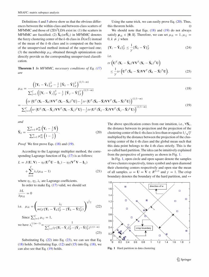
multiplied by the distance between the projection of the clus-tering center of the k-th class and the global mean such thatthis data point belongs to the k-th class strictly. This is theso-called hard partition. The idea can be intuitively explainedfrom the perspective of geometry as shown in Fig. 1.

In Fig. 1, open circle and open square denote the samplesof two clusters respectively, times symbol and open diamondtheir clustering centers respectively and open star the meanof all samples. ω = U = V ∈ R2×1 and γ = 1. The crispboundary denotes the boundary of the hard partition, and ↔

Fig. 1 Hard partition in data clustering

123

J. Gao et al.

is the area of the corresponding hard partition. The sampleswhich satisfy Eq. (25) are shown as filled circle. Obviously,we cannot use Eq. (19) to compute their corresponding mem-berships. However, in terms of their intuitive geometry, wecan use the hard partition to classify them. In other words,Fig. 1 demonstrates the rationale of the above specification.

On the other hand, Eqs. (19) and (25) reveal to us theimportance of a good choice of the parameterγ from twoaspects: (1) its value may determine the number of hard-partitioned samples; (2) its value may cause the hard partitionmore than once for some samples. For example, when γ →+0, all samples in Fig. 1 will be hard partitioned twice interms of Eq. (6). In the next subsection, we will investigatehow to choose an appropriate parameter γ .

3.2 Parameter γ

Equations (24) and (25) indicate that the parameter γ heav-ily determines the clustering results and plays a key rolein deciding whether a data point is hard partitioned or not.From the intuitive perspective, in order to avoid the phenom-enon that a data point is hard partitioned more than once,the distance between the projection of the data point andthe clustering center of the class must be less than or equalto 1/

√N (N ≥ 4) multiplied by the least distance between

the projection of the clustering centers of different classes.Theorem 2 will help us address the choice issue of the para-meter γ .

Theorem 2 Let Xi (i = 1, 2, . . . , n) be a sample, Xk bethe clustering center of the k-th class and X be the globalmean. And let γ = max{γ1, γ2, . . . , γC } in which γk =

N max j tr(UT (X j −X)VVT (X j −X)T U)

mink =k∗ tr(UT (Xk∗−Xk )VVT (Xk∗−Xk )T U)

for N ≥ 4, then Eq.

(25) can be rewritten as

tr(


)

≤ 1

Nmink∗ =k

tr(

UT (Xk∗ − Xk)VVT (Xk∗ − Xk)T U

). (26)

Proof According to Eq. (25), we have

tr(


)

≤ 1

γktr


). (27)

Substituting the prerequisite of the above theorem γk =N max j tr

(UT (X j −X)VVT (X j −X)T U

)

mink =k∗ tr(UT (Xk∗−Xk )VVT (Xk∗−Xk )

T U) into Eq. (7) and use

max j tr(UT (X j − X)VVT (X j − X)T U) ≥ tr(UT (Xk −X)VVT (Xk − X)T U), we immediately have Theorem 2.

Theorem 2 tells us clearly a selection rule which canbe used to determine an appropriate γ . Moreover, Eq. (26)reveals the influence of the parameter N on fuzzy clustering,

i.e., the bigger N is, the smaller the possibility of samplesbeing hard partitioned is and vice versa, which actually indi-cates that N determines the number of samples to be hardpartitioned during clustering. Therefore, with the increase inN , clustering will become fuzzier, while with the decreasein N , this method will gradually degenerate into a classicalhard clustering. In particular, N → 0, it becomes classicalhard clustering.

3.3 Direct computation of projection matrices U and V

Based on the proposed criterion MFMMC, we can derive astraightforward method of computing two projection matri-ces in Eq. (17) in an only-once computational way. In orderto do so, we rewrite αMFMMC and βMFMMC in Eq. (17) asαMFMMC

U /βMFMMCU and αMFMMC

V /βMFMMCV :

αMFMMCU

= tr

(UT (

C∑

k=1

n∑

i=1

μmik(Xi − Xk)VVT (Xi − Xk)

T )U

)

= tr(UT SVwU) (28)

βMFMMCU

= tr

(UT (

C∑

k=1

n∑

i=1

μmik(Xk − X)VVT (Xk − X)T )U

)

= tr(UT SVb U) (29)

αMFMMCV

= tr

(VT (

C∑

k=1

n∑

i=1

μmik(Xi − Xk)

T UUT (Xi − Xk))V

)

= tr(VT SUwV) (30)

βMFMMCV

= tr(VT

(C∑

k=1

n∑

i=1

μmik(Xk − X)T UUT (Xk − X))V

)

= tr(VT SUb V) (31)

where SVw(SU

w) is the fuzzy within-class scatter on the projec-tion matrix U(V), while SV

b (SUb ) is the fuzzy between-class

scatter on it. According to tr(AAT ) = tr(AT A), we knowthat αMFMMC

U and αMFMMCV (βMFMMC

U and βMFMMCV ) are dif-

ferent from each other only in their expressions and they areactually the same. Therefore, Eq. (17) can be transformedinto the following Eqs. (32) and (33):

arg maxUT U=Il1 ,VT V=Il2 ,�,ω

J (U, V)

= arg maxUT U=Il1 ,VT V=Il2 ,�,ω

βM F M MC

U − γαM F M MC

U

= arg maxUT U=Il1 ,VT V=Il2 ,�,ω

tr(UT (SVb − γ SV

w)U) (32)

123


arg maxVT V=Il2 ,UT U=Il1 ,�,ω

J (U, V)

= arg maxVT V=Il2 ,UT U=Il1 ,�,ω

βM F M MC

V − γαM F M MC

V

= arg maxVT V=Il2 ,UT U=Il1 ,�,ω

tr(VT (SUb − γ SU

w)V) (33)

Using the Lagrange multiplier method, Eqs. (32) and (33),we can get

(SVb − γ SV

w)U = λU (34)

(SUb − γ SU

w)V = λV (35)

In (Ye et al. 2004b), an iterative optimization method is usedto compute Eqs. (34) and (35) simultaneously. That is, wegive an initial to the projection matrices U and V and then usethe eigenvalue decomposition method to compute the projec-tion matrix U and V in Eqs. (34) and (35) respectively. Aftersubstituting the obtained U and V into Eqs. (34) and (35), weagain use the eigenvalue decomposition method to computethe new projection matrices U and V. Repeat this procedureuntil appropriate U and V are obtained. In this way, we canfinally obtain the projection matrices U and V in Eq. (17).

However, an open problem for the above minimizationprocedure is that we cannot guarantee its local and evenglobal convergence (Wang et al. 2007). Although anotheriterative method for solving the above matrices U and Vin (Wang et al. 2007) can be theoretically proved to belocally convergent (Wang and Wang 2009), it still keeps hightime/space complexities due to its iteration steps. Here onthe basis of matrix theories, we propose a direct methodwhich can compute effective approximate solutions to theabove matrices U and V with no iteration. This direct methodcan work well in the following way: Suppose U and Vare orthogonal. We can simplify the fuzzy scatter matri-ces SV

w, SUw, SV

b and SUb by dropping U and V, and then

we try to get the approximate solutions to Eqs. (34) and(35) through computing directly the unitary eigenvector ofthe corresponding matrix eigenvalue. No iteration is invokedin this method, thus decreasing the time/space complexitiesgreatly and therefore enhancing the efficiency of the projec-tion matrix computation.

Theorem 3 Suppose U and V are orthogonal matrices. Theeigenvalue decomposition method can be used to solve Eqs.(34) and (35).

Proof Since U and V are orthogonal matrices, SVw, SU

w, SVb

and SUb can be rewritten as

SV′w =

C∑

k=1

n∑

i=1

μmik(Xi − Xk)(Xi − Xk)

T (36)

SV′b =

C∑

k=1

n∑

i=1

μmik(Xk − X)(Xk − X)T (37)

SU′w =

C∑

k=1

n∑

i=1

μmik(Xi − Xk)

T (Xi − Xk) (38)

SU′b =

C∑

k=1

n∑

i=1

μmik(Xk − X)T (Xk − X) (39)

Let νi be the i-th column vector in U (or V), the originalproblems can be transformed into:

λ1 = arg maxυ1

υT1 (S

′b − γ S

′w)υ1 (40)

s.t. υT1 υ1 = 1

λk = arg maxυk

υTk (S

′b − γ S

′w)υk (41)

s.t.υT

k υ1 = υTk υ2 = · · · = υT

k υk−1 = 0υT

k υk = 1

From Eq. (40), we can find that υ1 is the eigenvector of themaximum eigenvalue of Sb−γ Sw, while νk can be computedby using the following Lagrange equation corresponding toEq. (41):

Lk = υTk (S

′b − γ S

′w)υk − λ(υT

k υk − 1) −k−1∑

q=1

λqυTk υq .

(42)

According to the necessary condition of the local optimalsolution, i.e., ∂Lk/∂υk = 0, we have

2(S′b − γ S

′w)υk − 2λυk −

k−1∑

q=1

λqυq = 0. (43)

Multiplying υTk on both sides of the above equation,

we have λ = λk = υTk (S

′b − γ S

′w)υk . Let λk−1 =

[λ1, . . . , λk]T , Qk−1 = [υ1, . . . ,υk−1], and multiplyυT

j ( j = 1, . . . , k − 1) on both sides of Eq. (43) such that

λk−1 = 2QTk−1(S

′b − γ S

′w)υk . (44)

Substituting Eq. (44) into Eq. (43), we get

(I − Qk−1QTk−1)(S

′b − γ S

′w)υk = λkυk . (45)

So, υk is just the unitary eigenvector of the maximal eigen-value of(I − Qk−1QT

k−1)(S′b − γ S

′w). Thus, this theorem

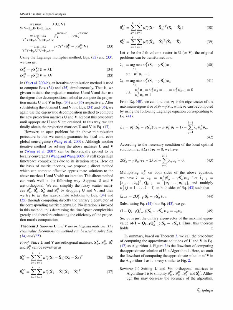
holds. ��In summary, based on Theorem 3, we call the procedure

of computing the approximate solutions of U and V in Eq.(17) as Algorithm-1. Figure 2 is the flowchart of computingthe approximate solution of U in Algorithm-1. Here, we omitthe flowchart of computing the approximate solution of V inthe Algorithm-1 as it is very similar to Fig. 2.

Remarks (1) Setting U and Vto orthogonal matrices inAlgorithm-1 is to simplify SV′

w , SU′w , SV′

b and SU′b . Altho-

ugh this may decrease the accuracy of the algorithm,

123

J. Gao et al.

Fig. 2 Flowchart ofAlgorithm-1 of calculating theapproximate solution of U

we can obtain certain findings as follows: As we mayknow well, when computing Eq. (17) by traditional iter-ative optimization methods (Ye et al. 2004b), we makeone projection matrix constant to compute the other one.In view of this, the algorithm is to replace the matrixUUT (VVT ) with unit matrix I.

(2) SinceSV′w , SU′

w , SV′b and SU′

b have been simplified, it isnot necessary for us to compute the approximate solutionto Eq. (17) using the corresponding iterative optimiza-tion method. In fact, we can compute it directly, whichcan greatly decrease the time/space complexities of thealgorithm.

(3) The solutions obtained by Algorithm-1 should be thesame as those in Definition 4, i.e., U ∈ Rm1×l1 and V ∈Rm2×l2 , rather than the complete orthogonal matricesunder the assumption.

3.4 Effective computation of the clustering center of Xk thek-th class

There is still a problem left to be solved, i.e., how to effec-tively compute the clustering center Xk of the k-th class indataset D. Xk affects not only the approximate solutions to

Eq. (17) but also the final clustering results. So, we need todiscuss how to define Xk .

In essence, the coexistence of the two-directional featureextraction matrices U and V in Eq. (17) makes it particularlydifficult to compute Xk directly through the computation ofthe necessary condition of Eq. (17). Luckily enough, we havesupposed U and V to be orthogonal in order to compute themeffectively. This inspires us further how to compute Xk .

Theorem 4 Let U and V be orthogonal matrices, the neces-sary condition of Eq. (17) is

Xk =∑n

i=1 μmik

(Xi − 1

γX

)

∑ni=1 μm

ik

(1 − 1

γ

) (46)

Proof Suppose V is an orthogonal matrix. In order to makeEq. (21) valid, in terms of Eq. (17), we must have

∂L

∂Xk= 0

i.e 2UTn∑

i=1

μmik(Xk − X)U = −2γ UT

n∑

i=1

μmik(Xi − Xk)U

(47)

123


Fig. 3 Flowchart of MSAFCalgorithm

Since U is an orthogonal matrix, we immediately have

n∑

i=1

μmik(Xk − X) = −γ

n∑

i=1

μmik(Xi − Xk) (48)

i.e.n∑

i=1

μmik(γ − 1)Xk =

n∑

i=1

μmik(γ Xi − X) (49)

So, Eq. (46) holds. ��From Theorem 4, we find that if U and V are orthogonal;

Eq. (17) is exactly the same as Eqs. (34) and (35). In termsof this fact, Xk , when satisfying Eq. (46), must be the nec-essary condition of Eqs. (34) and (35). That is, if we haveXk satisfying Eq. (46), with Algorithm-1 being executed, theobtained approximate solutions to the projection matrices areoptimal. Furthermore, after observing Eqs. (20) and (46), wemultiply both sides of Eq. (46) by UT and V and we canget the projection matrix Yk in Eq. (20). That is, Yk gotten

through feature extraction from the clustering center Xk ofthe k-th class in D is just the clustering center of the k-thclass in S. As we know, this strategy has been used widelyin supervised feature extraction methods (Li and Yuan 2005;Zhang and Zhou 2005; Ye et al. 2004b; Wang et al. 2008).One of its advantages is that the global intrinsic structure ofsource samples can be preserved as much as possible duringfeature extraction. Therefore, this strategy can not only real-ize unsupervised feature extraction but also keep the globalintrinsic structure of original samples.

Based on all the analyses above, we obtain the proposedalgorithm MSAFC which can be summarized by the flow-chart in Fig. 3.

4 Experimental results

In this section, we examine the performances of the proposedalgorithm MSAFC on both clustering and unsupervised

123

J. Gao et al.

feature extraction for matrix data. The computing platformofour experiments is Vista, Inter Core2 T5500 1.66G CPU,1.5G memory and the simulation package matlab 7.0. Ourexperimental results are reported in three subsections. Sec-tion 4.1 helps us observe the clustering performances of theproposed algorithm in comparatively small datasets, whileSect. 4.2 is for comparatively large datasets. In Sects. 4.3and 4.4, we will demonstrate the capability of unsupervisedfeature extraction of the proposed algorithm by running iton a face dataset and a gene dataset which are both of highdimensionality.

4.1 MSAFC for clustering on comparatively small datasets

4.1.1 Datasets

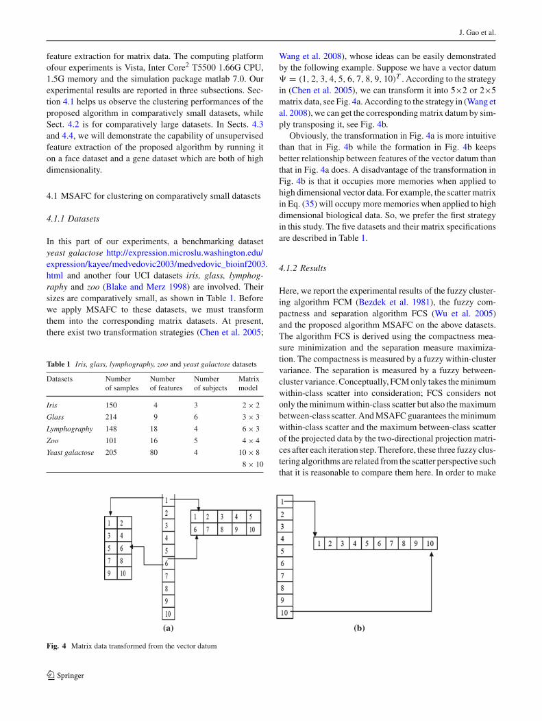
In this part of our experiments, a benchmarking datasetyeast galactose http://expression.microslu.washington.edu/expression/kayee/medvedovic2003/medvedovic_bioinf2003.html and another four UCI datasets iris, glass, lymphog-raphy and zoo (Blake and Merz 1998) are involved. Theirsizes are comparatively small, as shown in Table 1. Beforewe apply MSAFC to these datasets, we must transformthem into the corresponding matrix datasets. At present,there exist two transformation strategies (Chen et al. 2005;

Table 1 Iris, glass, lymphography, zoo and yeast galactose datasets

Datasets Number Number Number Matrixof samples of features of subjects model

Iris 150 4 3 2 × 2

Glass 214 9 6 3 × 3

Lymphography 148 18 4 6 × 3

Zoo 101 16 5 4 × 4

Yeast galactose 205 80 4 10 × 8

8 × 10

Wang et al. 2008), whose ideas can be easily demonstratedby the following example. Suppose we have a vector datum� = (1, 2, 3, 4, 5, 6, 7, 8, 9, 10)T . According to the strategyin (Chen et al. 2005), we can transform it into 5×2 or 2×5matrix data, see Fig. 4a. According to the strategy in (Wang etal. 2008), we can get the corresponding matrix datum by sim-ply transposing it, see Fig. 4b.

Obviously, the transformation in Fig. 4a is more intuitivethan that in Fig. 4b while the formation in Fig. 4b keepsbetter relationship between features of the vector datum thanthat in Fig. 4a does. A disadvantage of the transformation inFig. 4b is that it occupies more memories when applied tohigh dimensional vector data. For example, the scatter matrixin Eq. (35) will occupy more memories when applied to highdimensional biological data. So, we prefer the first strategyin this study. The five datasets and their matrix specificationsare described in Table 1.

4.1.2 Results

Here, we report the experimental results of the fuzzy cluster-ing algorithm FCM (Bezdek et al. 1981), the fuzzy com-pactness and separation algorithm FCS (Wu et al. 2005)and the proposed algorithm MSAFC on the above datasets.The algorithm FCS is derived using the compactness mea-sure minimization and the separation measure maximiza-tion. The compactness is measured by a fuzzy within-clustervariance. The separation is measured by a fuzzy between-cluster variance. Conceptually, FCM only takes the minimumwithin-class scatter into consideration; FCS considers notonly the minimum within-class scatter but also the maximumbetween-class scatter. And MSAFC guarantees the minimumwithin-class scatter and the maximum between-class scatterof the projected data by the two-directional projection matri-ces after each iteration step. Therefore, these three fuzzy clus-tering algorithms are related from the scatter perspective suchthat it is reasonable to compare them here. In order to make

Fig. 4 Matrix data transformed from the vector datum

123

http://expression.microslu.washington.edu/expression/kayee/medvedovic2003/medvedovic_bioinf2003.html




Table 2 Clustering accuracies (mean ± std %) on iris, glass, lymphography, zoo and yeast galactose datasets

Algorithms Datasets

Iris Glass Lymphography Zoo Yeast galactose

FCM 0.893 ± 0 0.7117 ±0 0.5820 ±0 0.8141 ± 2.33 0.85567 ± 0

FCS 0.90667 ± 0 0.7000 ± 0 0.5859 ± 0 0.8618 ± 0 0.87463 ± 1.54

MSAFC 0.95749 ± 0(l1 = 2, l2 = 1)

0.73831 ± 2.5(l1 = 3, l2 = 2)

0.5927 ± 1.87(l1 = 4, l2 = 1)

0.9031 ± 1.7(l1 = 3, l2 = 4)

0.98581 ± 0.28(10 × 8)(l1 = 3, l2 = 4)

0.97512 ± 1.3(8 × 10)(l1 = 2, l2 = 5)

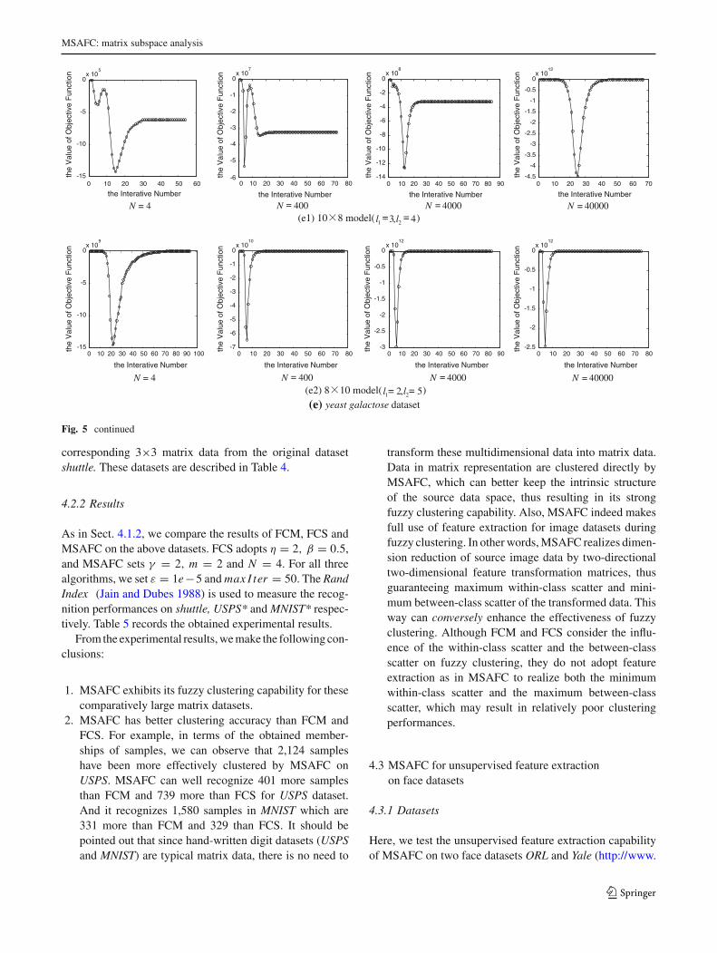
our comparison fair, we set ε = 1e−5 and maxIter = 100 anduse initfcm function in Matlab 7.0 to generate initial mem-berships for all these three algorithms. We use the mean andvariance of the clustering indices Rand Index (Jain and Dubes1988) after 100 runs of every algorithm on every dataset as thefinal clustering result. In addition, FCS has two parameters,i.e., η controlling the trade-off between the within-class scat-ter and the between-class scatter and β controlling the fuzzypartition. We set η = 2, β = 0.5 for FCS, and γ = 2, m = 2and N = 40,000 for MSAFC. Table 2 illustrates the obtainedclustering results. Figures 5 and 6 demonstrate the influenceof the parameter N = 4, 400, 4,000, 40,000 on the conver-gence and fuzzy partitions of MSAFC on the five datasetsrespectively. Figure 7 demonstrates the clustering results ofMSAFC with N = 40,000 on the five datasets having differ-ent extracted features and matrix data from these datasets.

From the above experimental results, we can easilyobserve the followings:

1. The clustering accuracies in Table 2 tell us that the pro-posed algorithm MSAFC has stronger clustering capa-bility. In particular, when dealing with high dimensionalgene data, MSAFC can achieve considerably satisfactoryclustering results provided that the proper matrix rep-resentation and column (row) projection matrices U ∈Rm1×l1(V ∈ Rm2×l2) are adopted. This fact shows thatthe use of matrix representation in MSAFC does notdecrease the clustering effectiveness when dealing withtraditional vector data.

2. Figure 5 shows the convergence of MSAFC when per-forming it on iris dataset with l1 = 2, l2 = 1, glassdataset with l1 = 3, l2 = 2, lymphography dataset withl1 = 4, l2 = 1, zoo dataset with l1 = 3, l2 = 4, yeastgalactose dataset (10 × 8) with l1 = 3, l2 = 4 and yeastgalactose dataset (8 × 10) with l1 = 2, l2 = 5. Wecan observe from this figure that MSAFC always con-verges before the maximum iterations (max I ter = 100)

is reached. In other words, it always converges with thetermination condition |J (U, V)(p+1) − J (U, V)p| ≤ ε.Furthermore, let us compare several special cases [i.e,

iris dataset (N = 4), glass dataset (N = 400), lymphog-raphy dataset (N = 4) and yeast galactose dataset with10×8 model (N = 4) and so on] with all other conver-gences. We can easily find that although MSAFC canconverge, it cannot guarantee to be convergent to a localoptimal value.

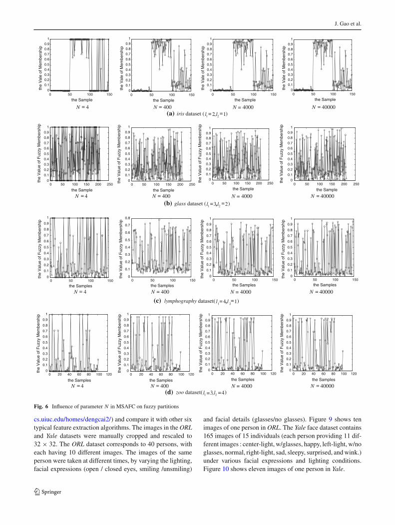
3. It can be easily seen from Fig. 6 and Table 3 that theparameter N has great influence on the fuzzy partitionsgenerated by MSAFC on the datasets. For iris dataset,when N is set as 4, 400, and 4,000, there exist 135,24, and 2 samples respectively out of the total 150samples that are hard partitioned. When N = 40,000,no sample is hard partitioned. For glass dataset, whenN = 4, 98 samples out of the total 214 ones arehard partitioned, and no sample does so when N =400, 4,000, 40,000. Similar observations can be obtainedfor other datasets. This fact is fully in accordance withTheorem 2. Meanwhile, we can observe that with theincrease in N , the obtained clustering accuracy willbecome better or at least equivalent. For example, for irisdataset, when N = 4, the clustering accuracy is 0.92671,and when N = 400, 4,000, 40,000, the clustering accu-racy achieves 0.95749. For glass dataset, when N =4,400, 4,000, 40,000, the clustering accuracy becomes0.7012, 0.7111, 0.7255, 0.7278, respectively.

4. It can be easily seen from Fig. 7 that the clustering resultsof MSAFC on the datasets depend on the extracted fea-tures and the adopted matrix data from the datasets.

4.2 MSAFC for clustering on comparatively large datasets

4.2.1 Datasets

In this subsection, we report the clustering performancesof MSAFC on comparatively large datasets. The adopteddatasets include one UCI dataset shuttle and two hand-writtendigit datasets USPS with 9,286 16 × 16 image samples andMINIST with 4,000 28 × 28 image samples (http://www.cs.uiuc.edu/homes/dengcai2/) (See Fig. 8). For USPS and MIN-

123

http://www.cs.uiuc.edu/homes/dengcai2/


J. Gao et al.

0 2 4 6 8 10 12-6000

-5000

-4000

-3000

-2000

-1000

0

the Iterative Number

the

Val

ue o

f Obj

ect F

unct

ion

0 5 10 15 20 25 30 35 40 45-3

-2.5

-2

-1.5

-1

-0.5

0x 10

7

the Interative Number

the

Val

ue o

f Obj

ect F

unct

ion

0 5 10 15 20 25 30 35 40 45 50-10

-9

-8

-7

-6

-5

-4

-3

-2

-1

0x 10

8


the

Val

ue o

f Obj

ect F

unct

ion

0 5 10 15 20 25 30 35 40 45-14

-12

-10

-8

-6

-4

-2

0x 10

8


the

Val

ue o

f Obj

ect F

unct

ion

4N 400N 4000N 40000N

(a) iris dataset ( 1,2 21 ll )

0 5 10 15 20 25-8

-7

-6

-5

-4

-3

-2

-1

0x 10

8


the

Val

ue o

f Obj

ect F

unct

ion

0 10 20 30 40 50 60 70 80 90 100-12

-10

-8

-6

-4

-2

0x 10

6


the

Val

ue o

f Obj

ect F

unct

ion

0 10 20 30 40 50 60 70 80-4.5

-4

-3.5

-3

-2.5

-2

-1.5

-1

-0.5

0x 10

10

the Interative Numberth

e V

alue

of O

bjec

t Fun

ctio

n0 10 20 30 40 50 60 70

-6

-5

-4

-3

-2

-1

0x 10

11


the

Val

ue o

f Obj

ect F

unct

ion

4N 400N 4000N 40000N

(b) glass dataset ( 23 21 ll , )

0 5 10 15 20 25 30-14

-12

-10

-8

-6

-4

-2

0x 10

4


the

Val

ue o

f Obj

ectiv

e F

unct

ion

0 10 20 30 40 50 60 70-4.5

-4

-3.5

-3

-2.5

-2

-1.5

-1

-0.5

0x 10

7


the

Val

ue o

f Obj

ectiv

e F

unct

ion

0 10 20 30 40 50 60-2.5

-2

-1.5

-1

-0.5

0x 10

9


the

Val

ue o

f Obj

ectiv

e F

unct

ion

0 20 40 60 80 100 120-12

-10

-8

-6

-4

-2

0x 10

13


the

Val

ue o

f Obj

ectiv

e F

unct

ion

4N 400N 4000N 40000N

(c) lymphography dataset( 14 21 ll , )

0 10 20 30 40 50 60 70 80 90 100-3

-2.5

-2

-1.5

-1

-0.5

0x 10

6


the

Val

ue o

f Obj

ectiv

e F

unct

ion

0 10 20 30 40 50 60-14

-12

-10

-8

-6

-4

-2

0x 10

8


the

Val

ue o

f Obj

ectiv

e F

unct

ion

0 10 20 30 40 50 60 70 80-16

-14

-12

-10

-8

-6

-4

-2

0x 10

8


the

Val

ue o

f Obj

ectiv

e F

unct

ion

0 20 40 60 80 100 120-3

-2.5

-2

-1.5

-1

-0.5

0x 10

10


the

Val

ue o

f Obj

ectiv

e F

unct

ion

(d) zoo dataset( 4,3 21 ll )

= = = =

= = = =

= = = =

= =

= =

= =

= =

4N 400N 4000N 40000N= = = =

Fig. 5 Convergence of MSAFC

IST datasets, we randomly selected 2500 and 2160 imagesamples from them to form two datasets USPS* and MNIST*,respectively. We trained MSAFC on USPS* and MNIST*,

and then use the obtained clustering results on USPS*and MNIST* to test the recognition power on the wholeUSPS and MINIST datasets. Note that we have adopted the

123


0 10 20 30 40 50 60-15

-10

-5

0x 10

5


the

Val

ue o

f Obj

ectiv

e F

unct

ion

0 10 20 30 40 50 60 70 80-6

-5

-4

-3

-2

-1

0x 10

7


the

Val

ue o

f Obj

ectiv

e F

unct

ion

0 10 20 30 40 50 60 70 80 90-14

-12

-10

-8

-6

-4

-2

0x 10

8


the

Val

ue o

f Obj

ectiv

e F

unct

ion

0 10 20 30 40 50 60 70-4.5

-4

-3.5

-3

-2.5

-2

-1.5

-1

-0.5

0x 10

12


the

Val

ue o

f Obj

ectiv

e F

unct

ion

(e1) 10 8 model( 4,3 21 ll )

0 10 20 30 40 50 60 70 80 90 100-15

-10

-5

0x 10

9


the

Val

ue o

f Obj

ectiv

e F

unct

ion

0 10 20 30 40 50 60 70 80-7

-6

-5

-4

-3

-2

-1

0x 10

10


the

Val

ue o

f Obj

ectiv

e F

unct

ion

0 10 20 30 40 50 60 70 80 90-3

-2.5

-2

-1.5

-1

-0.5

0x 10

12

the Interative Numberth

e V

alue

of O

bjec

tive

Fun

ctio

n

0 10 20 30 40 50 60 70 80-2.5

-2

-1.5

-1

-0.5

0x 10

12


the

Val

ue o

f Obj

ectiv

e F

unct

ion

(e2) 8 10 model( 5,2 21 ll )

(e) yeast galactose dataset

4N 400N 4000N 40000N= = = =

= =4N 400N 4000N 40000N= = = =

= =

Fig. 5 continued

corresponding 3×3 matrix data from the original datasetshuttle. These datasets are described in Table 4.

4.2.2 Results

As in Sect. 4.1.2, we compare the results of FCM, FCS andMSAFC on the above datasets. FCS adopts η = 2, β = 0.5,and MSAFC sets γ = 2, m = 2 and N = 4. For all threealgorithms, we set ε = 1e−5 and max I ter = 50. The RandIndex (Jain and Dubes 1988) is used to measure the recog-nition performances on shuttle, USPS* and MNIST* respec-tively. Table 5 records the obtained experimental results.

From the experimental results, we make the following con-clusions:

1. MSAFC exhibits its fuzzy clustering capability for thesecomparatively large matrix datasets.

2. MSAFC has better clustering accuracy than FCM andFCS. For example, in terms of the obtained member-ships of samples, we can observe that 2,124 sampleshave been more effectively clustered by MSAFC onUSPS. MSAFC can well recognize 401 more samplesthan FCM and 739 more than FCS for USPS dataset.And it recognizes 1,580 samples in MNIST which are331 more than FCM and 329 than FCS. It should bepointed out that since hand-written digit datasets (USPSand MNIST) are typical matrix data, there is no need to

transform these multidimensional data into matrix data.Data in matrix representation are clustered directly byMSAFC, which can better keep the intrinsic structureof the source data space, thus resulting in its strongfuzzy clustering capability. Also, MSAFC indeed makesfull use of feature extraction for image datasets duringfuzzy clustering. In other words, MSAFC realizes dimen-sion reduction of source image data by two-directionaltwo-dimensional feature transformation matrices, thusguaranteeing maximum within-class scatter and mini-mum between-class scatter of the transformed data. Thisway can conversely enhance the effectiveness of fuzzyclustering. Although FCM and FCS consider the influ-ence of the within-class scatter and the between-classscatter on fuzzy clustering, they do not adopt featureextraction as in MSAFC to realize both the minimumwithin-class scatter and the maximum between-classscatter, which may result in relatively poor clusteringperformances.

4.3 MSAFC for unsupervised feature extractionon face datasets

4.3.1 Datasets

Here, we test the unsupervised feature extraction capabilityof MSAFC on two face datasets ORL and Yale (http://www.

123


J. Gao et al.

0 50 100 1500

0.1

0.2

0.3

0.40.5

0.6

0.7

0.80.9

1

the Sample

the

Val

e of

Mem

bers

hip

0 50 100 1500

0.1

0.2

0.3

0.4

0.5

0.6

0.7

0.8

0.9

1

the Sample

the

Val

e of

Mem

bers

hip

0 50 100 1500

0.1

0.2

0.3

0.40.5

0.6

0.7

0.80.9

1

the Sample

the

Val

e of

Mem

bers

hip

0 50 100 1500

0.10.20.30.40.5

0.60.70.80.9

1

the Sample

the

Val

e of

Mem

bers

hip

4N 400N 4000N 40000N(a) iris dataset ( 1,2 21 ll )

0 50 100 150 200 2500

0.1

0.2

0.3

0.4

0.5

0.6

0.7

0.8

0.9

1

the Sample

the

Val

ue o

f Fuz

zy M

embe

rshi

p

0 50 100 150 200 2500

0.1

0.2

0.3

0.4

0.5

0.6

0.7

0.8

0.9

1

the Sample

the

Val

ue o

f Fuz

zy M

embe

rshi

p

0 50 100 150 200 2500

0.1

0.2

0.3

0.40.5

0.6

0.7

0.80.9

1

the Sample

the

Val

ue o

f Fuz

zy M

embe

rshi

p

0 50 100 150 200 2500

0.1

0.2

0.3

0.4

0.5

0.6

0.7

0.8

0.9

1

the Sample

the

Val

ue o

f Fuz

zy M

embe

rshi

p

(b) glass dataset ( 23 21 ll , )

0 50 100 1500

0.1

0.2

0.3

0.4

0.5

0.6

0.7

0.8

0.9

1

the Samples

the

Val

ue o

f Fuz

zy M

embe

rshi

p

0 50 100 1500

0.1

0.2

0.3

0.4

0.5

0.6

0.7

0.8

the Samples

the

Val

ue o

f Fuz

zy M

embe

rshi

p

0 50 100 1500

0.1

0.2

0.3

0.4

0.5

0.6

0.7

0.8

0.9

1

the Samples

the

Val

ue o

f Fuz

zy M

embe

rshi

p

0 50 100 1500

0.1

0.2

0.3

0.4

0.5

0.6

0.7

0.8

0.9

1

the Samplesth

e V

alue

of F

uzzy

Mem

bers

hip

(c) lymphography dataset( 14 21 ll , )

0 20 40 60 80 100 1200

0.1

0.2

0.3

0.4

0.5

0.6

0.7

0.8

0.9

1

the Samples

the

Val

ue o

f Fuz

zy M

embe

rshi

p

0 20 40 60 80 100 1200

0.1

0.2

0.3

0.4

0.5

0.6

0.7

0.8

0.9

1

the Samples

the

Val

ue o

f Fuz

zy M

embe

rshi

p

0 20 40 60 80 100 1200

0.1

0.2

0.3

0.4

0.5

0.6

0.7

0.8

0.9

1

the Samples

the

Val

ue o

f Fuz

zy M

embe

rshi

p

0 20 40 60 80 100 1200

0.1

0.2

0.3

0.4

0.5

0.6

0.7

0.8

0.9

1

the Samples

the

Val

ue o

f Fuz

zy M

embe

rshi

p

(d) zoo dataset( 4,3 21 ll )

= = = == =

4N 400N 4000N 40000N= = = =

4N 400N 4000N 40000N= = = =

4N 400N 4000N 40000N= = = =

= =

= =

= =

Fig. 6 Influence of parameter N in MSAFC on fuzzy partitions

cs.uiuc.edu/homes/dengcai2/) and compare it with other sixtypical feature extraction algorithms. The images in the ORLand Yale datasets were manually cropped and rescaled to32 × 32. The ORL dataset corresponds to 40 persons, witheach having 10 different images. The images of the sameperson were taken at different times, by varying the lighting,facial expressions (open / closed eyes, smiling /unsmiling)

and facial details (glasses/no glasses). Figure 9 shows tenimages of one person in ORL. The Yale face dataset contains165 images of 15 individuals (each person providing 11 dif-ferent images : center-light, w/glasses, happy, left-light, w/noglasses, normal, right-light, sad, sleepy, surprised, and wink.)under various facial expressions and lighting conditions.Figure 10 shows eleven images of one person in Yale.

123



0 50 100 150 200 2500

0.1

0.2

0.3

0.4

0.5

0.6

0.7

0.8

0.9

1

the Samples

the

Val

ue o

f Fuz

zy M

embe

rshi

p

0 50 100 150 200 2500

0.1

0.2

0.3

0.4

0.5

0.6

0.7

0.8

0.9

1

the Samples

the

Val

ue o

f Fuz

zy M

embe

rshi

p

0 50 100 150 200 2500

0.1

0.2

0.3

0.4

0.5

0.6

0.7

0.8

0.9

1

the Samples

the

Val

ue o

f Fuz

zy M

embe

rshi

p

0 50 100 150 200 2500

0.1

0.2

0.3

0.4

0.5

0.6

0.7

0.8

0.9

1

the Samples

the

Val

ue o

f Fuz

zy M

embe

rshi

p

(e1) 10 8 model( 4,3 21 ll )

0 50 100 150 200 2500

0.1

0.2

0.3

0.4

0.5

0.6

0.7

0.8

0.9

1

the Samples

the

Val

ue o

f Fuz

zy M

embe

rshi

p

0 50 100 150 200 2500

0.1

0.2

0.3

0.4

0.5

0.6

0.7

0.8

0.9

1

the Samples

the

Val

ue o

f Fuz

zy M

embe

rshi

p

0 50 100 150 200 2500

0.1

0.2

0.3

0.4

0.5

0.6

0.7

0.8

0.9

1

the Samplesth

e V

alue

of F

uzzy

Mem

bers

hip

0 50 100 150 200 2500

0.1

0.2

0.3

0.4

0.5

0.6

0.7

0.8

0.9

1

the Samples

the

Val

ue o

f Fuz

zy M

embe

rshi

p

(e2) 8 10 model( 5,2 21 ll )

(e) yeast galactose dataset

4N 400N 4000N 40000N= = = == =

4N 400N 4000N 40000N= = = == =

Fig. 6 continued

4.3.2 Results

In this experiment, we have adopted six typical feature extrac-tion algorithms PCA (Sirovich and Kirby 1987), ICA (Yuenand Lai 2002), FLDC (Li et al. 2011), 2DPCA (Yang et al.2004), (2D)2PCA (Zhang and Zhou 2005) and GPCA (Ye etal. 2004a) to conduct a comparative study for MSAFC. Inorder to make our comparison fair, we adopt the same exper-imental setting as described in the references about these sixalgorithms. In particular, FDLC has a regularization

In order to do a comparative study on the recognition per-formances of these algorithms for the corresponding test-ing datasets, we take the first 2, 3, 4 and 5 samples ofeach individual in the dataset for training, and the remain-ing samples for testing. Five-fold cross validation is usedto carry out our experiment here. Also, after unsupervisedfeature extraction, PCA, ICA and FLDC generate the corre-sponding p-dimensional subspace, 2DPCA the correspond-ing 32 × dsubspace, and (2D)2PCA, GPCA, and MSAFCthe corresponding d × d(d2) subspace. The 1-NN classifieris used to determine the class label of a testing sample. Therecognition performances (i.e. recognition accuracies) of allthese algorithms on ORL and Yale datasets are respectivelyillustrated in Tables 6 and 7 in which dim denotes the numberof dimensions for brevity and time the running time in sec-onds used by the corresponding eigenvalue decomposition.Figure 11 reports the recognition performance of MSAFC on

different number of training samples from the ORL and Yaledatasets.

From the above experimental results on face recognitiondatasets, we have the following observations:

1. In term of the recognition accuracy and the number ofextracted features, Tables 6 and 7 show that MSAFChas higher feature extraction capability compared tothe other unsupervised feature extraction methods. Thisindicates that fuzzification indeed helps MSAFC betterreflect the real-world images, e.g. in strong or weak light-ing, thus increasing the accuracy of feature extraction(Kw and Pedry 2005). Although FLDC is also based onthe fuzzy concept, its effectiveness is not as good as thatof MSAFC. This is because FLDC can only deal withdata in vector representation and does not consider thefully intrinsic geometric structure in face image datasets.Particularly, like FCM and FCS, it gets relatively low sep-arable degree of samples when dealing with data havinga large number of high dimensional images. That is, themembership of each sample, which decides which classthe sample belongs to, is almost the same, thus decreas-ing its efficiency in feature extraction. However, MSAFCmakes good use of the result of feature extraction to com-pute the membership of the samples in each step of iter-ations and at the same time the samples with differentmemberships obtained from the last step of calculation

123

J. Gao et al.

11.2

1.41.6

1.82

1

1.5

20.92

0.93

0.94

0.95

0.96

0.97

clumnrow

the

Mea

n of

Acc

urac

y

11.5

22.5

3

11.5

22.5

30.66

0.68

0.7

0.72

0.74

clumnrow

the

Mea

n of

Acc

urac

y

(a) iris dataset (b) glass dataset

11.5

22.5

3

0

2

4

60.52

0.54

0.56

0.58

0.6

0.62

clumnrow

the

Me

an o

f A

ccur

acy

12

34

1

2

3

40.84

0.86

0.88

0.9

0.92

clumnrow

the

Mea

n of

Acc

urac

y

(c) lymphography (d)tesatad zoo dataset

02

46

8

0

5

100.75

0.8

0.85

0.9

0.95

1

clumnrow

the

Mea

n of

Acc

urac

y

02

46

810

02

46

80.75

0.8

0.85

0.9

0.95

1

clumnrow

the

Me

an o

f A

ccur

acy

10 88 10 (e) yeast galactose dataset

Fig. 7 Clustering results of MSAFC on the datasets with different extracted features and matrices

Table 3 Influence of parameter N in MSAFC on fuzzy partitions in which H-Samples denotes hard partitioned samples

N N = 4 N = 400 N = 4,000 N = 40,000

Datasets Number of theH-Samples

Accuracy Number of theH-Samples



Accuracy

Iris 135 0.9261 24 0.95749 2 0.95749 0 0.95749

Glass 98 0.7012 0 0.71110

0.7255 0 0.7288

Lymphography 50 0.5856 0 0.6014 0 0.6081 0 0.6284

Zoo 61 0.8586 0 0.8913 0 0.9010 0 0.9109

Yeast galactose 10 × 8 94 0.9847 0 0.9847 0 0.9847 0 0.9902

8 × 10 180 0.9756 0 0.97972 0 0.97972 0 0.9805

123


50 100 150 200 250 300

10

20

30

40

50

60

50 100 150 200 250 300 350 400 450 500 550

102030405060708090

100110

(a) USPS (b) MNIST

Fig. 8 Samples of handwritten digits from 0 to 9

Table 4 Shuttle, USPS* and MNIST* datasets

Datasets Number Number Number Matrixof samples of features of subjects model

Shuttle 14,500 9 7 3 × 3

USPS*/USPS 2,500 256 10 16 × 16

MNIST*/MNIST 2,160 784 10 28 × 28

Table 5 Recognition performance comparison on shuttle, USPS andMNIST datasets

Algorithms Datasets

Shuttle USPS MNIST

FCM 0.4267 0.5540 0.5821

FCS 0.46295 0.6890 0.5830

MSAFC 0.5666 0.84953 0.73552(l1 = 3, l2 = 1) (l1 = 2, l2 = 10) (l1 = 19, l2 = 3)

are used to guide the direction of feature extraction. Theadvantage of doing so is that since fuzzy clustering inour method is based on the data after feature extraction,the separable degrees measured by the memberships ofhigh dimensional image samples is increased to a certainextent. Furthermore, such degrees show us the contribu-tions of different samples to the results of the subsequentfeature extraction step.

2. In term of the running time in eigenvalue decomposition,our Algorithm-1 is obviously practical and efficient forits use in computing U and V in Eq. (17). For example,the running time of Algorithm-1 is generally only 1/300

of that of FCA or ICA, and FLDC may even take 1,000times longer than that of Algorithm-1. Besides, we havealso tried the iterative method in (Wang et al. 2007) andits running time is about 1,000 times as much as that ofthe Algorithm-1.

3. From Fig. 9, we can find that the recognition accuracyincreases as the number of training samples goes up, thusshowing a clear relationship between the result of featureextraction and the number of training samples and thiscoincides with the basic characteristic of unsupervisedfeature extraction methods. In particular, from the curvetendency in Fig. 9, the recognition accuracy of MSAFCdoes not change much after achieving its optimal featureextraction. This fact reveals that it has better adaptabilityand robustness than others.

parameter r ∈ [0, 1] (Li et al. 2011) which controls thewithin-class scatter Srw = rSw + (1 − r)diag(Sw) usedin FDLC such that it is not singular. We take FDLC withr = 0.1 and MSAFC with γ = 2, m = 2 and N = 4. Wealso set ε = 1e − 5, max I ter = 30 and use initfcm functionin Matlab 7.0 to generate initial memberships for both FDLCand MSAFC.

4.4 MSAFC for unsupervised feature extractionon gene datasets

4.4.1 Datasets

In order to observe the superior unsupervised feature extrac-tion performances of MSAFC, we adopt two very high

50 100 150 200 250 300

51015202530

Fig. 9 All images of a certain class in ORL dataset

50 100 150 200 250 300 350

51015202530

Fig. 10 All images of a certain class in Yale dataset

123

J. Gao et al.

Table 6 Recognition performance on ORL dataset

Dataset ORL

Number of training samples 2 3 4 5

Algorithm Accuracy (Dim) Time (s) Accuracy (Dim) Time (s) Accuracy (Dim) Time (s) Accuracy (Dim) Time (s)

PCA 0.6938 (73) 16.7701 0.71786 (121) 15.9121 0.80417 (156) 14.8201 0.84 (201) 14.2117

ICA 0.6625 (59) 17.6391 0.70659 (132) 15.8932 0.775 (156) 16.5549 0.825 (224) 13.5834

FLDC 0.6938 (214) 59.264 0.7250 (276) 56.16 0.82083 (403) 63.753 0.855 (446) 64.975

2DPCA 0.71875 (13x32) 0.014 0.76429 (18x32) 0.014 0.8625 (14x32) 0.015 0.89 (7x32) 0.014

(2D)2PCA 0.72188 (102) 0.017 0.76786 (192) 0.016 0.8667 (182) 0.016 0.905 (182) 0.018

GPCA 0.7250 (182) 0.016 0.7714 (132) 0.014 0.8667 (162) 0.017 0.8990 (212) 0.017

MSAFC 0.72813 (202) 0.019 0.7750 (182) 0.024 0.8708 (172) 0.029 0.905 (172) 0.034

Table 7 Recognition performance on Yale dataset

Dataset Yale

Number of Training Samples 2 3 4 5

Algorithm Accuracy (Dim) Time (s) Accuracy (Dim) Time (s) Accuracy (Dim) Time (s) Accuracy (Dim) Time (s)

PCA 0.4222 (29) 18.1741 0.45 (44) 17.4409 0.52381 (57) 17.1757 0.5778 (74) 16.6297

ICA 0.46667 (41) 16.3674 0.48889 (53) 18.5562 0.56333 (57) 17.9625 0.61333 (79) 15.4739

FLDC 0.4444 (189) 59.906 0.45 (153) 57.843 0.54286 (340) 62.285 0.6 (249) 59.748

2DPCA 0.5778 (7x32) 0.015 0.63333 (7x32) 0.016 0.67619 (6x32) 0.014 0.71111 (7x32) 0.015

(2D)2PCA 0.5778 (72) 0.016 0.63333 (82) 0.015 0.68571 (82) 0.015 0.71111 (82) 0.017

GPCA 0.5778 (72) 0.015 0.64167 (92) 0.014 0.68571 (72) 0.016 0.72353 (82) 0.015

MSAFC 0.5778 (82) 0.051 0.64167 (72) 0.062 0.69524 (82) 0.073 0.73333 (62) 0.079

0 5 10 15 20 25 30 350.1

0.2

0.3

0.4

0.5

0.6

0.7

0.8

0.9

1

Dimension

Rco

gniti

on A

ccur

acy

2 Train3 Train4 Train5 Train

0 5 10 15 20 25 30 350.1

0.2

0.3

0.4

0.5

0.6

0.7

0.8

Dimension

Rec

ogni

tion

Acc

urac

y

2 Train3 Train4 Train5 Train

(a) ORL (b)tesatad Yale dataset

Fig. 11 Performance of MSAFC with different numbers of training samples in each dataset

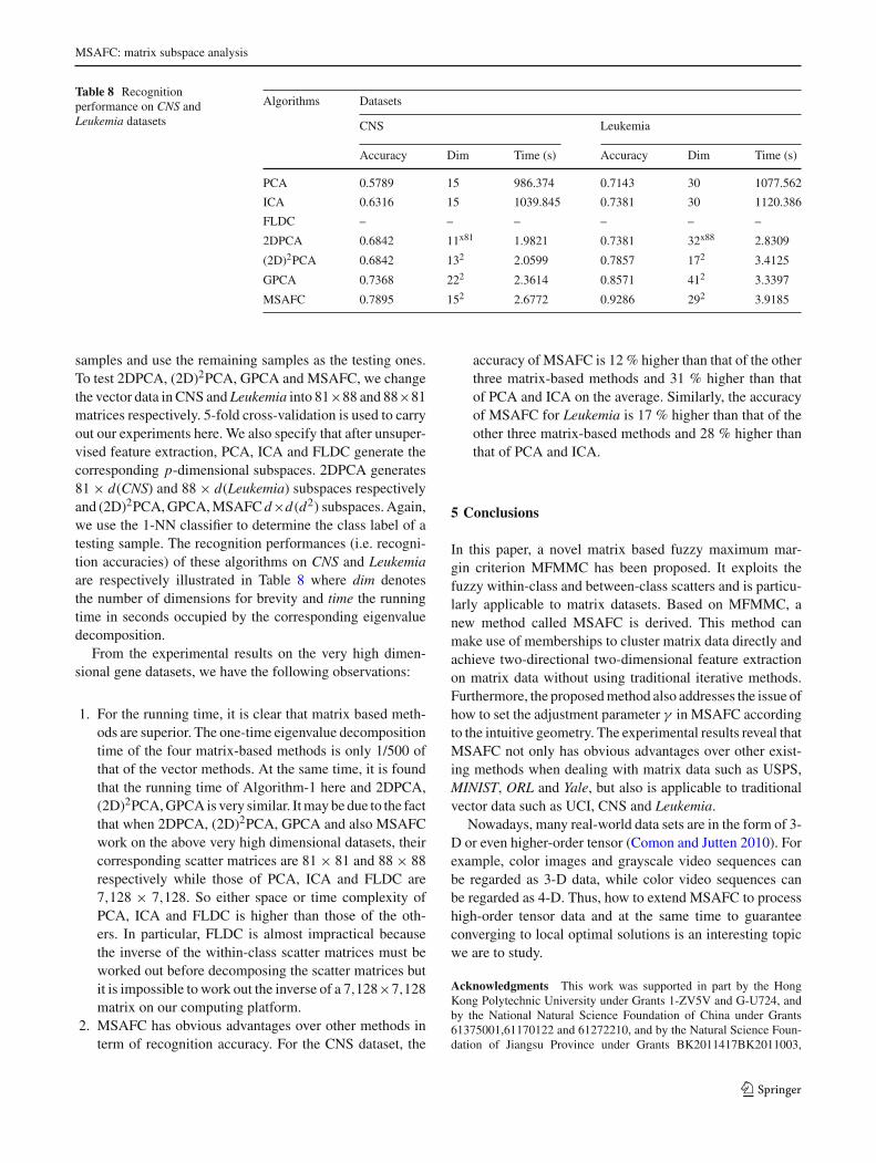
dimensional gene datasets, namely, CNS and Leukemia(Chung et al. 2006). CNS consists of 34 samples in which 25are positive and 9 negative and each sample has 7,128 fea-tures; Leukemia includes 72 samples in which 47 are positiveand 25 negative with each sample having 7,128 features.

4.4.2 Experimental results

In this experiment, we adopt the same methods and parame-ter settings as in Sect. 4.3.2. We randomly select 15 samplesfrom CNS and 30 samples from Leukemia as the training

123


Table 8 Recognitionperformance on CNS andLeukemia datasets

Algorithms Datasets

CNS Leukemia

Accuracy Dim Time (s) Accuracy Dim Time (s)

PCA 0.5789 15 986.374 0.7143 30 1077.562

ICA 0.6316 15 1039.845 0.7381 30 1120.386

FLDC – – – – – –

2DPCA 0.6842 11x81 1.9821 0.7381 32x88 2.8309

(2D)2PCA 0.6842 132 2.0599 0.7857 172 3.4125

GPCA 0.7368 222 2.3614 0.8571 412 3.3397

MSAFC 0.7895 152 2.6772 0.9286 292 3.9185

samples and use the remaining samples as the testing ones.To test 2DPCA, (2D)2PCA, GPCA and MSAFC, we changethe vector data in CNS and Leukemia into 81×88 and 88×81matrices respectively. 5-fold cross-validation is used to carryout our experiments here. We also specify that after unsuper-vised feature extraction, PCA, ICA and FLDC generate thecorresponding p-dimensional subspaces. 2DPCA generates81 × d(CNS) and 88 × d(Leukemia) subspaces respectivelyand (2D)2PCA, GPCA, MSAFC d×d(d2) subspaces. Again,we use the 1-NN classifier to determine the class label of atesting sample. The recognition performances (i.e. recogni-tion accuracies) of these algorithms on CNS and Leukemiaare respectively illustrated in Table 8 where dim denotesthe number of dimensions for brevity and time the runningtime in seconds occupied by the corresponding eigenvaluedecomposition.

From the experimental results on the very high dimen-sional gene datasets, we have the following observations:

1. For the running time, it is clear that matrix based meth-ods are superior. The one-time eigenvalue decompositiontime of the four matrix-based methods is only 1/500 ofthat of the vector methods. At the same time, it is foundthat the running time of Algorithm-1 here and 2DPCA,(2D)2PCA, GPCA is very similar. It may be due to the factthat when 2DPCA, (2D)2PCA, GPCA and also MSAFCwork on the above very high dimensional datasets, theircorresponding scatter matrices are 81 × 81 and 88 × 88respectively while those of PCA, ICA and FLDC are7,128 × 7,128. So either space or time complexity ofPCA, ICA and FLDC is higher than those of the oth-ers. In particular, FLDC is almost impractical becausethe inverse of the within-class scatter matrices must beworked out before decomposing the scatter matrices butit is impossible to work out the inverse of a 7,128×7,128matrix on our computing platform.

2. MSAFC has obvious advantages over other methods interm of recognition accuracy. For the CNS dataset, the

accuracy of MSAFC is 12 % higher than that of the otherthree matrix-based methods and 31 % higher than thatof PCA and ICA on the average. Similarly, the accuracyof MSAFC for Leukemia is 17 % higher than that of theother three matrix-based methods and 28 % higher thanthat of PCA and ICA.

5 Conclusions

In this paper, a novel matrix based fuzzy maximum mar-gin criterion MFMMC has been proposed. It exploits thefuzzy within-class and between-class scatters and is particu-larly applicable to matrix datasets. Based on MFMMC, anew method called MSAFC is derived. This method canmake use of memberships to cluster matrix data directly andachieve two-directional two-dimensional feature extractionon matrix data without using traditional iterative methods.Furthermore, the proposed method also addresses the issue ofhow to set the adjustment parameter γ in MSAFC accordingto the intuitive geometry. The experimental results reveal thatMSAFC not only has obvious advantages over other exist-ing methods when dealing with matrix data such as USPS,MINIST, ORL and Yale, but also is applicable to traditionalvector data such as UCI, CNS and Leukemia.

Nowadays, many real-world data sets are in the form of 3-D or even higher-order tensor (Comon and Jutten 2010). Forexample, color images and grayscale video sequences canbe regarded as 3-D data, while color video sequences canbe regarded as 4-D. Thus, how to extend MSAFC to processhigh-order tensor data and at the same time to guaranteeconverging to local optimal solutions is an interesting topicwe are to study.

Acknowledgments This work was supported in part by the HongKong Polytechnic University under Grants 1-ZV5V and G-U724, andby the National Natural Science Foundation of China under Grants61375001,61170122 and 61272210, and by the Natural Science Foun-dation of Jiangsu Province under Grants BK2011417BK2011003,

123

J. Gao et al.

JiangSu 333 expert engineering Grant (BRA2011142), and 2011, 2012&2013 Postgraduate Student’s Creative Research Fund of JiangsuProvince. Also, we are very thankful for the referees whose commentshelp us greatly improve the quality of the paper.

References

Bezdek JC (1981) Pattern recognition with fuzzy objective functionalgorithms. Plenum Press, New York

Bian ZQ, Zhang XG (2001) Pattern Recogn. TsingHua University Press,Beijing

Blake CL, Merz CJ (1998) UCI Rrepository of Machine Learning Data-bases”, Irvine, CA: University of California, Department of Infor-mation and Computer Science. http://www.ics.uci.edu/~mlearn/MLRepository.html

Chen SC, Zhu YL, Zhang DQ (2005) Feature extraction approachesbased on matrix pattern: MatPCA and MatFLDA. Pattern RecognLett 26:1157–1167

Choi JY, Park MS (2009) Theoretical analysis on feature extractioncapability of class-augmented PCA. Pattern Recogn 42(2):2353–2362

Chung FL, Wang ST et al (2006) Clustering analysis of gene expressiondata based on semi-supervised clustering algorithm. Soft Comput10(5):981–994

Comon P, Jutten C (2010) Handbook of blind source separation,independent component analysis and applications. Academic Press,New York

Cui GQ, Gao W (2005) Face recognition based on two-layer generatevirtual data for SVM. Chin J Comput 28(3):368–376

Daizhan Cg, June F, Hongli L (2013) Solving fuzzy relational equationsvia semi-tensor product. IEEE Trans Fuzzy Syst on-line availablenow

Fisher RA (1936) The use of multiple measurements in taxonomic prob-lems. Ann Eugenics 7:179–188

Fu Y, Yuan JS, Li Z, Huang TS, Wu Y (2007) Query-driven locallyadaptive Fisher faces and expert-model for face recognition. In: Pro-ceedings of the International Conference on Image Processing 2007,pp 141–144

Gao J, Wang ST (2009) Fuzzy maximum scatter difference discriminantcriterion based clustering algorithm. J Softw 20(11):2939–2949

Hsieh P, Wang D, Hsu C (2006) A linear feature extraction for multiclassclassification problems based on class mean and covariance discrim-inant information. IEEE Trans Pattern Anal Mach Intell 28(6):223–235

Jain A, Dubes R (1988) Algorithms for clustering data. Prentice Hall,Upper Saddle River

Jing XY, Wong HS, Zhang D (2006) Face recognition based on 2DFisherface approach. Pattern Recogn 39:707–710

Jolliffe IT (1986) Principal Component Analysis. Springer, New YorkKim YD, Choi S (2007) Color face tensor factorization and slicing

for illumination-robust recognition. In: Proceedings of intrenationalconference on biometrics, pp 19–28

Kim E, Park M, Kim S, Park M (1998) A transformed input-domainapproach to fuzzy modeling. IEEE Trans Fuzzy Syst 6(4):596–604

Kw KC, Pedry W (2005) Face recognition using a fuzzy Fisher classifier.Pattern Recogn 38(10):1717–1732

Lei Z, Chu R, He R, Liao S, Li SZ (2007) Face recognition by discrim-inant analysis with Gabor tensor representation. In: Proceedings ofinternational conference on biometrics, pp 87–95

Li M, Yuan B (2005) 2D-LDA: a statistical linear discriminant analysisfor image matrix. Pattern RecognLett 26:527–532

Li H, Jiang T, Zhang K (2006) Efficient and robust feature extractionby maximum margin criterion. IEEE Trans Neural Netw 17(1):157–165

Li J, Zhang L, Tao D, Sun H, Zhao D (2009) A prior neurophysiologicknowledge free tensor-based scheme for single trial egg classifica-tion. IEEE Trans Neural Syst Rehabilit Eng 17(2):107–115

Li CH, Kuo BC, Lin CT (2011) LDA-based clustering algorithm and itsapplication to an unsupervised feature extraction. IEEE Trans FuzzySyst 19(1):152–162

Liu J, Tan XY, Zhang DQ (2007) Comments on efficient and robustfeature extraction by maximum margin criterion. IEEE Trans NeuralNetw 18(6):1862–1864

Lu HP, Plataniotis KN, Venetsanopoulos AN (2008) MPCA: multilinearprincipal component analysis of tensor objects. IEEE Trans NeuralNetw 19(1):18–39

Lu HP, Plataniotis KN, Venetsanopoulos AN (2009) Uncorrelated mul-tilinear discriminant analysis with regularization and aggregationfor tensor object recognition. IEEE Trans Neural Netw 20(1):103–123

Lu HP, Plataniotis KN, Venetsanopoulos AN (2011) A survey of multi-linear subspace learning for tensor data. Pattern Recogn 44(7):1540–1551

Martínez AM, Kak AC (2001) PCA versus LDA. IEEE Trans PatternAnal Mach Intell 23(2):228–233

Panagakis Y, Kotropoulos C, Arce GR (2010) Non-negative multilinearprincipal component analysis of auditory temporal modulations formusic genre classification. In: IEEE transaction on audio, speech,and language processing 18(3):576–588

Peng J, Zhang P, Riedel N (2008) Discriminant learning analysis. IEEETrans Syst Man Cybern Part B 38(6):1614–1625

Ren CX, Dai DQ (2010) Incremental learning of bidirectional principalcomponents for face recognition. Pattern Recogn 143(1):318–330

Sirovich L, Kirby M (1987) Low-dimensional procedure for character-ization of human faces. J Optical Soc Am 4:519–524

Song FX, Zhang D, Yang JY, Gao XM (2006) Adaptive classicationalgorithm based on maximum scatter difference discriminant crite-rion. Acta Automatica Sinica 32(2):541–549

Tao D, Li X, Wu X, Maybank SJ (2007) General tensor discriminantanalysis and Gabor features for gait recognition. IEEE Trans PatternAnal Mach Intell 29(10):1700–1715

Turk M, Pentland A (1991) Eigenfaces for recognition. J Cogn Neurosci3(1):71–86

Wang JG, Yang WK, Lin YS, Yang JY (2008) Two-directional max-imum scatter difference discriminant analysis for face recognition.Neurocomputing 72(1–3):352–358

Wang X, Tang X (2004) A unified framework for subspace face recog-nition. IEEE Trans Pattern Anal Mach Intell 26(9):1223–1228

Wang Z, Chen SC, Liu J, Zhang DQ (2008) Pattern representation in fea-ture extraction and classification—matrix versus vector. IEEE TransNeural Netw 19:758–769

Wang F, Wang X (2009) Neighborhood discriminant tensor mapping.Neurocomputing 72(7–9):2035–2039

Wang H, Yan SC, Huang TS, Tang XO (2007) A convengent solutionto tensor subspace learning. IN: Proceedings of IJCAI, pp 629–634

Wu KL, Yu K, Yang MS (2005) A novel fuzzy clustering algorithmbased on a fuzzy scatter matrix with optimality tests. Pattern RecognLett 26(4):639–652

Xiong HL, Swanmy MNS, Ahmad MO (2005) Two-dimensional FLDfor face recognition. Pattern Recogn 38:1121–1124

Yan S, Xu D, Yang Q, Zhang L, Tang X, Zhang H (2007) Multilineardiscriminant analysis for face recognition. IEEE Trans Image Process16(1):212–220

Yang WK, Yan H, Wang JG, Yang JY (2008) Face recognition usingcomplete Fuzzy LDA. In: Proceedings of ICPR, pp 1–4

Yang WK, Yan XY, Zhang L, Sun CY (2010) Feature extraction basedon fuzzy 2DLDA. Neurocomputing 73(10–12):1556–1561

Yang J, Zhang D, Frangi AF, Yang JY (2004) Two-dimensional PCA:a new approach to appearance-based face representation and recog-nition. IEEE Trans Pattern Anal Mach Intell 26(1):131–137

123

http://www.ics.uci.edu/~mlearn/MLRepository.html

http://www.ics.uci.edu/~mlearn/MLRepository.html


Ye JP, Janardan R, Li Q (2004a) GPCA: an efficient dimension reduc-tion scheme for image compression and retrieval. In: Proceedingsof the tenth ACM SIGKDD international conference on knowledgediscovery and data mining, pp 354–363

Ye JP, Janardan R, Li Q (2004b) Two-dimensional linear discriminantanalysis. In: Proceedings of advances in neural information process-ing systems

Ye JP (2005) Generalized low rank approximations of matrices. MachLearn 61(1–3):167–191

Ye JH, Liu ZG (2009) Multi-modal face recognition based on localbinary pattern and Fisherfaces. Comput Eng 35(11):193–195

Yuen PC, Lai JH (2002) Face representation using independent compo-nent analysis. Pattern Recogn 35(6):1247–1257

Zhang DQ, Zhou ZH (2005) (2D)2PCA: two-directional two-dimensional PCA for efficient face representation and recognition.Neurocomputing 69(1–3):224–231

Zheng W, Zou C, Zhao L (2005) Weighted maximum margin discrim-inant analysis with kernels. Neurocomputing 67:357–362

123

Documents

MSAFC: matrix subspace analysis with fuzzy clustering ability