MSc THESIS - Publicationce-publications.et.tudelft.nl/publications/300_implementing_texture... · MSc THESIS Implementing Texture Feature Extraction Algorithms on FPGA Mahshid Roumi

Computer EngineeringMekelweg 4,

2628 CD DelftThe Netherlands

http://ce.et.tudelft.nl/

2009

MSc THESIS

Implementing Texture Feature ExtractionAlgorithms on FPGA

Mahshid Roumi

Abstract

Faculty of Electrical Engineering, Mathematics and Computer Science

CE-MS-2009-25

Feature extraction is a key function in various image processing ap-plications. A feature is an image characteristic that can capturecertain visual property of the image. Texture is an important fea-ture of many image types, which is the pattern of information orarrangement of the structure found in a picture. Texture featuresare used in different applications such as image processing, remotesensing and content-based image retrieval. These features can beextracted in several ways. The most common way is using a GrayLevel Co-occurrence Matrix (GLCM). GLCM contains the second-order statistical information of neighboring pixels of an image. Tex-tural properties can be calculated from GLCM to understand thedetails about the image content. However, the calculation of GLCMis very computationally intensive. In this thesis, an FPGA accel-erator for fast calculation of GLCM is designed and implemented.We propose an FPGA-based architecture for parallel computation ofsymmetric co-occurrence matrices. Experimental results show thatour approach improves 2x up to 4x the processing time for simulta-neous computation of sixteen co-occurrence matrices.


THESIS

submitted in partial fulfillment of therequirements for the degree of

MASTER OF SCIENCE

in

COMPUTER ENGINEERING

by

Mahshid Roumiborn in Tehran, Iran

Computer EngineeringDepartment of Electrical EngineeringFaculty of Electrical Engineering, Mathematics and Computer ScienceDelft University of Technology


by Mahshid Roumi

Abstract

Feature extraction is a key function in various image processing applications. Afeature is an image characteristic that can capture certain visual property of theimage. Texture is an important feature of many image types, which is the pattern

of information or arrangement of the structure found in a picture. Texture features areused in different applications such as image processing, remote sensing and content-basedimage retrieval. These features can be extracted in several ways. The most common wayis using a Gray Level Co-occurrence Matrix (GLCM). GLCM contains the second-orderstatistical information of neighboring pixels of an image. Textural properties can becalculated from GLCM to understand the details about the image content. However,the calculation of GLCM is very computationally intensive. In this thesis, an FPGAaccelerator for fast calculation of GLCM is designed and implemented. We propose anFPGA-based architecture for parallel computation of symmetric co-occurrence matrices.Experimental results show that our approach improves 2x up to 4x the processing timefor simultaneous computation of sixteen co-occurrence matrices.

Laboratory : Computer EngineeringCodenumber : CE-MS-2009-25

Committee Members :

Advisor: Dr. Ir. Georgi Gaydadjiev , CE, TU Delft

Advisor: Dr. Ir. A. Shahbahrami , CE, TU Delft

Chairperson: Dr. Koen Bertels , CE, TU Delft

Member: Dr. Ir. Zaid Al-Ars , CE, TU Delft

Member: Dr. Ir. Rene van Leuken, ENS, TU Delft

i

ii

To My Parents and my Brother for their unconditional love andendless support

iii

iv

Contents

List of Figures viii

List of Tables ix

Acknowledgements xi

1 Introduction 11.1 Motivation . . . . . . . . . . . . . . . . . . . . . . . . . . . . . . . . . . . 11.2 Project Goals . . . . . . . . . . . . . . . . . . . . . . . . . . . . . . . . . . 11.3 Thesis Organization . . . . . . . . . . . . . . . . . . . . . . . . . . . . . . 1

2 Digital Images and Texture Features 32.1 Digital Image . . . . . . . . . . . . . . . . . . . . . . . . . . . . . . . . . . 32.2 Image Analysis . . . . . . . . . . . . . . . . . . . . . . . . . . . . . . . . . 42.3 Texture . . . . . . . . . . . . . . . . . . . . . . . . . . . . . . . . . . . . . 5

2.3.1 Introduction of Texture . . . . . . . . . . . . . . . . . . . . . . . . 52.3.2 Texture Analysis . . . . . . . . . . . . . . . . . . . . . . . . . . . . 62.3.3 Application of Texture . . . . . . . . . . . . . . . . . . . . . . . . . 72.3.4 Texture Feature Extraction Algorithms . . . . . . . . . . . . . . . 82.3.5 Rules for Choosing Texture Extraction Algorithms . . . . . . . . . 132.3.6 Statistical Algorithms for Texture Extraction . . . . . . . . . . . . 142.3.7 Comparison between Co-occurrence and others Algorithms . . . . 262.3.8 Computational Overhead of Co-occurrence Processing . . . . . . . 27

3 Related Work 29

4 FPGA Implementation 374.1 FPGA . . . . . . . . . . . . . . . . . . . . . . . . . . . . . . . . . . . . . . 37

4.1.1 FPGA vs ASIC . . . . . . . . . . . . . . . . . . . . . . . . . . . . . 374.2 Hardware Target . . . . . . . . . . . . . . . . . . . . . . . . . . . . . . . . 384.3 Proposed Design . . . . . . . . . . . . . . . . . . . . . . . . . . . . . . . . 384.4 Results . . . . . . . . . . . . . . . . . . . . . . . . . . . . . . . . . . . . . . 414.5 Comparison with Related Work . . . . . . . . . . . . . . . . . . . . . . . . 44

5 Conclusion and Future Work 515.1 Conclusions . . . . . . . . . . . . . . . . . . . . . . . . . . . . . . . . . . . 515.2 Future Work . . . . . . . . . . . . . . . . . . . . . . . . . . . . . . . . . . 52

Bibliography 53

v

vi

List of Figures

2.1 Some examples of texture features. . . . . . . . . . . . . . . . . . . . . . . 62.2 Texture classification [44]. . . . . . . . . . . . . . . . . . . . . . . . . . . . 62.3 Texture segmentation [23]. . . . . . . . . . . . . . . . . . . . . . . . . . . . 72.4 Different steps in image analysis process. . . . . . . . . . . . . . . . . . . . 72.5 Example of first-order methods. . . . . . . . . . . . . . . . . . . . . . . . . 162.6 Diagram of angles, the Haralick texture features are calculated in each of

these directions. . . . . . . . . . . . . . . . . . . . . . . . . . . . . . . . . . 172.7 An image of size 4× 4. . . . . . . . . . . . . . . . . . . . . . . . . . . . . . 212.8 Gray tone color . . . . . . . . . . . . . . . . . . . . . . . . . . . . . . . . . 212.9 The symmetrical horizontal GLCM. . . . . . . . . . . . . . . . . . . . . . 222.10 4× 4 rotated image. . . . . . . . . . . . . . . . . . . . . . . . . . . . . . . 26

3.1 System architecture for calculation GLCM texture features [43]. . . . . . . 303.2 Block diagram of extraction Haralick features [43]. . . . . . . . . . . . . . 313.3 Algorithm for the classification of prostate tissue cancer [4]. . . . . . . . . 323.4 System model [4]. . . . . . . . . . . . . . . . . . . . . . . . . . . . . . . . . 323.5 Block diagram of calculation GLCM on FPGA [4]. . . . . . . . . . . . . . 333.6 Overview of the FPGA architecture [5]. . . . . . . . . . . . . . . . . . . . 343.7 Overview of the FPGA architecture [4]. . . . . . . . . . . . . . . . . . . . 36

4.1 Different distances with four different directions, which have been used tocalculate sixteen GLCMs. . . . . . . . . . . . . . . . . . . . . . . . . . . . 39

4.2 Proposed model. . . . . . . . . . . . . . . . . . . . . . . . . . . . . . . . . 394.3 Overview of the input and output BRAMs for the image size 32× 32 and

Ng = 32. . . . . . . . . . . . . . . . . . . . . . . . . . . . . . . . . . . . . . 404.4 Architectures of BRAMs for Ng = 32. . . . . . . . . . . . . . . . . . . . . 414.5 Processing units. . . . . . . . . . . . . . . . . . . . . . . . . . . . . . . . . 424.6 Frequency and clock period Ng = 32. . . . . . . . . . . . . . . . . . . . . . 424.7 Frequency and clock period Ng = 64. . . . . . . . . . . . . . . . . . . . . . 434.8 Frequency and clock period Ng = 128. . . . . . . . . . . . . . . . . . . . . 434.9 Processing times(µs)for different image dimensions and various Ng by

using various FPGA devices. . . . . . . . . . . . . . . . . . . . . . . . . . 444.10 Comparison of processing times (µs) with Ng = 32. . . . . . . . . . . . . . 444.11 Comparison of processing times (µs) with Ng = 64. . . . . . . . . . . . . . 454.12 Comparison of processing times (µs) with Ng = 128. . . . . . . . . . . . . 454.13 Processing times (µs) with limitation of number of occurs for 128 × 128

image. . . . . . . . . . . . . . . . . . . . . . . . . . . . . . . . . . . . . . . 464.14 Area utilizations Ng = 32. . . . . . . . . . . . . . . . . . . . . . . . . . . . 464.15 a) Area utilizations. . . . . . . . . . . . . . . . . . . . . . . . . . . . . . . 464.16 b) Area utilizations. . . . . . . . . . . . . . . . . . . . . . . . . . . . . . . 474.17 c) Area utilizations. . . . . . . . . . . . . . . . . . . . . . . . . . . . . . . 474.18 Area utilizations Ng = 64. . . . . . . . . . . . . . . . . . . . . . . . . . . . 47

vii

4.19 a) Area utilizations. . . . . . . . . . . . . . . . . . . . . . . . . . . . . . . 484.20 b) Area utilizations. . . . . . . . . . . . . . . . . . . . . . . . . . . . . . . 484.21 Area utilizations Ng = 128. . . . . . . . . . . . . . . . . . . . . . . . . . . 484.22 a) Area utilizations. . . . . . . . . . . . . . . . . . . . . . . . . . . . . . . 494.23 b) Area utilization. . . . . . . . . . . . . . . . . . . . . . . . . . . . . . . . 49

viii

List of Tables

2.1 Construction of co-occurrence matrix. . . . . . . . . . . . . . . . . . . . . 22

4.1 Virtex-XC2VP30. . . . . . . . . . . . . . . . . . . . . . . . . . . . . . . . . 384.2 Virtex-XC4VfX60. . . . . . . . . . . . . . . . . . . . . . . . . . . . . . . . 384.3 Virtex-XC5VLX330. . . . . . . . . . . . . . . . . . . . . . . . . . . . . . . 384.4 Processing times (µs) achieved for various input image dimensions using

various FPGA devices. Iakovidis et al [4]. . . . . . . . . . . . . . . . . . . 494.5 a) Comparison the processing time (µs) our result with the Iakovidis et

al results . . . . . . . . . . . . . . . . . . . . . . . . . . . . . . . . . . . . . 504.6 b) Comparison the processing time (µs) our result with the Iakovidis et

al results . . . . . . . . . . . . . . . . . . . . . . . . . . . . . . . . . . . . . 504.7 c) Comparison the processing time (µs) our result with the Iakovidis et

al results . . . . . . . . . . . . . . . . . . . . . . . . . . . . . . . . . . . . . 50

ix

x

Acknowledgements

First of all, I am grateful to my parents, and my brother for their unlimited and uncon-ditional love, encouragement and support in my whole life.My special thanks goes to my supervisor Dr. Georgi Gaydadjiev for his patience, time,and help.Special thanks also to Dr. Asad Shahbahami for his advice, support, and encouragementduring my MSc project.My special thanks goes to all my friends warmly for their support in all aspects duringmy time in Delft. I cannot forget my great time in Delft with them.I would also like to thank all CE members for their support, and I am thankful to youtoo.

Mahshid RoumiDelftAugust 2009

xi

xii

Introduction 1Akey function in different image applications is feature extraction. A feature is a

characteristic that can capture a certain visual property of an image either globallyfor the whole image, or locally for objects or regions. Different features such as

color, shape, and texture can be extricated from an image. Texture is the variation ofdata at different scales. A number of methods have been developed for texture featureextraction. They can be extracted from co-occurrence matrices and wavelet transformcoefficients. There after, they are stored as feature vectors.

In this thesis we focus on calculating the co-occurrence matrices. As calculating thismatrix and features are time consuming, we design a dedicated hardware on FPGA forthis purpose.

This chapter is organized as follows. Section 1.1 presents the motivation for thiswork. Our project goals are identified in Section 1.2. Section 1.3 describes the thesisorganization.

1.1 Motivation

There are different algorithms to extract texture features such as structural, statistical,and transform domain. The structural approaches provide symbolic description for animage. The statistical approaches provide texture features by distribution and relation-ships between the gray levels of an image. In addition, texture features can be extractedusing transform coefficients such as wavelet transform coefficients.

1.2 Project Goals

• To investigate different approaches to extract texture features extraction,

• To evaluate the co-occurrence matrix as a suitable technique for texture featureextraction. In addition, to investigate the computation of this matrix,

• To design dedicated hardware to speedup the calculation of the co-occurrence ma-trix and extracting features from it.

• To use three platforms FPGA to compare their results and performances.

1.3 Thesis Organization

The thesis is organized as follows. In Chapter 2, we discuss the basic information aboutdigital image processing, texture features and different techniques that can be used for

1

2 CHAPTER 1. INTRODUCTION

texture feature extraction. We present related work in Chapter 3 followed by hardwareimplementation in Chapter 4. We present the summary and the future work in Chapter 5.Last chapter is bibliography.

Digital Images and TextureFeatures 2This chapter contains an overview of a digital image, and texture. Section 2.1 describesthe digital image. Image analysis is defines in section Section 2.2. The following sectionswill provide a discussion about texture and different methods to extract texture features.

2.1 Digital Image

An image is defined as a two dimensional function, f(x, y), where x and y are spatialcoordinates, and f(x, y) is a set of G grey-tones. When x, y and the grey-tones of fhave discrete quantities, the image is called a digital image [14].

The function f(x, y) is [14]:

f(x, y) =

f(0, 0) f(0, 1) · · · f(0, Ny − 1)f(1, 0) f(1, 1) · · · f(1, Ny − 1)· · · · · · · · · · · ·· · · · · · · · · · · ·

f(Nx − 1, 0) f(Nx − 1, 1) · · · f(Nx − 1, Ny − 1)

(2.1)

A digital image has a finite number of elements, each of these elements has a particularvalue and location. These elements are called pixel or image elements [14].

Digital image has a different types, some of them are [45]:

• Binary image:

This is the simplest type of image with two gray-values, 0 and 1 or black andwhite. Each pixel is represented by a single bit. These types of images are usefulin computer vision applications where only information about images or outlinesare required. It can be created from gray-scale image that uses 0 for pixels withgray levels below the threshold and 1 for other pixel but this way of creation is notuseful because most of the information is lost and the image result are smaller.

• Gray-scale image:

These images contain the brightness information. The number of bits that are usedto represent each pixel, are related to the number of different brightness levelsavailable. The typical image contains 8 bits per pixel so there are 256 differentpossible gray-tones (Ng) or intensity values from 0 to 255.

• Color image:

Normally, images are represented as RGB (Red, Green, Blue) models, and eachpixel has 24 bits. The brightness information and color information are coupledand represented in many applications. These two information are septated bytransferring RGB information to the mathematical.

3

4 CHAPTER 2. DIGITAL IMAGES AND TEXTURE FEATURES

Digital image can be presented in different ways. The first way is plot image as asurface with three dimensions (x, y, z), in which x, y are spatial coordinates, and z isthe value of the f(x, y). In the second way, the image is shown as a visual intensityarray. There are just three intensity values, 0 (black), 0.5 (gray), 1 (white). In the thirdmethod, the image is represented as a 2D array. This is useful when the size of the imageis big and one part of it needs to be analyzed.

2.2 Image Analysis

Image analysis considers the image for a specific application and it is useful in many ap-plications such as computer vision, medical imaging, and pattern recognition. It extractsthe useful information from the image. The image analysis involves image segmentation,image transformation, pattern classification, and feature extraction [45]. Some of theseconcepts are explained in the remainder of this chapter.

• Image segmentation: Image segmentation divides the input image into multiplesegments or regions, which show objects or meaningful parts of objects. It segmentsimage into homogenous regions thus making it easier to analyze images.

• Image transformation: Image transform is used to find the spatial frequency infor-mation that can be used in the feature extraction step.

• Feature extraction: Large amounts of data are used to represent an image, sothe analysis of an image needs a large amount of memory and thus takes moretime. In order to reduce the amount of data, an image is represented using a set offeatures. Feature extraction is a primitive type of pattern recognition and it is veryimportant for pattern recognition. This step extract some features such as color,shape, and texture. Features contain the relevant information of an image and willbe used in image processing (e.g. searching, retrieval, storing). It decomposes intotwo parts, feature construction and feature selection.

Features are divided into different classes based on the kind of properties theydescribe. Some important features are as follows.

– Color:From a mathematical viewpoint the color signal is an extension from scalar-signals to vector-signals. The color can be represented by an average color(three scalars) or a color histogram (three functions). Color features can bederived from a histogram of the image. The multi-dimensional histogramis used for the multi-color image [32]. From a brightness histogram, thecolor features are derived as RGB components. Color features are useful forbiomedical image processing, such as for cell classification, and cancer celldetection [32]. The weakness is that the color histogram of two differentthings with the same color, are equal.

– Texture:

2.3. TEXTURE 5

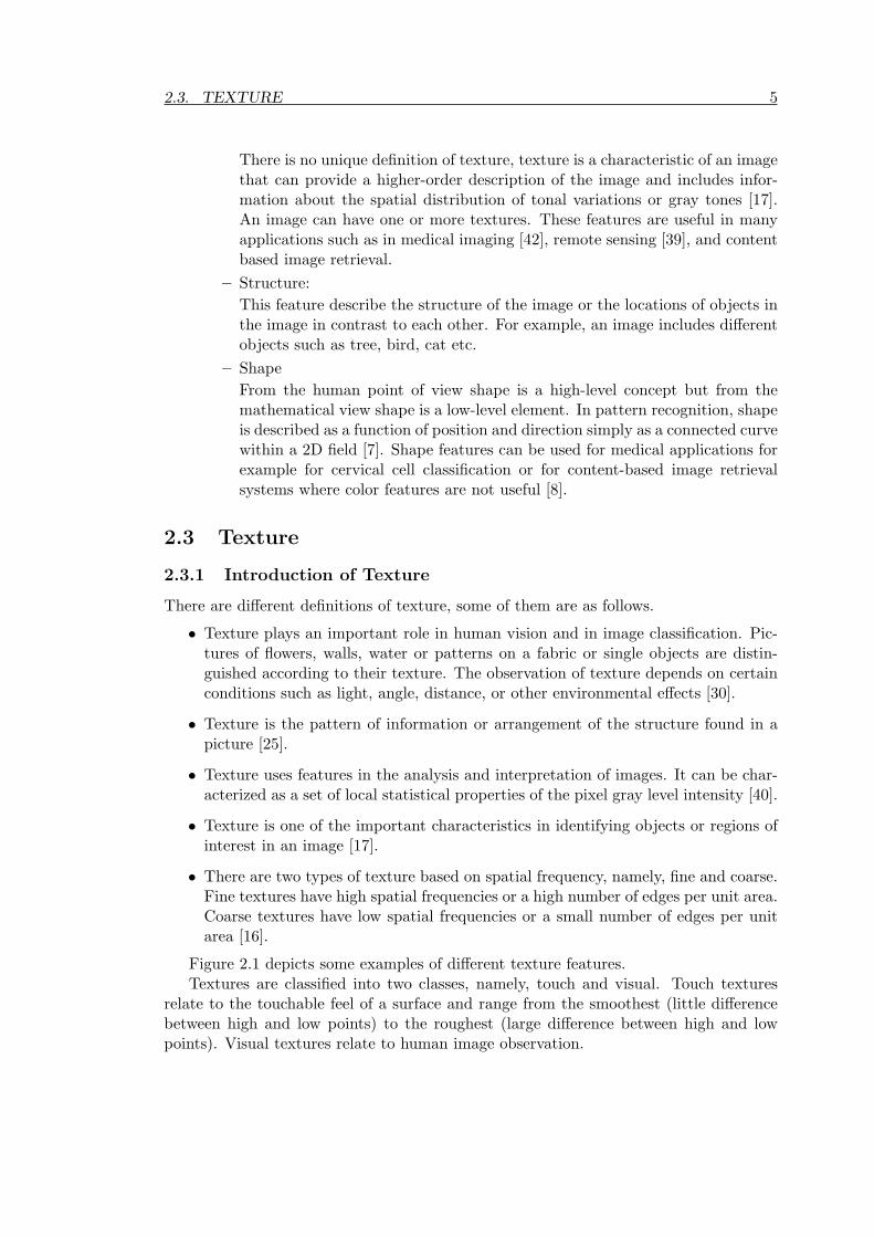
There is no unique definition of texture, texture is a characteristic of an imagethat can provide a higher-order description of the image and includes infor-mation about the spatial distribution of tonal variations or gray tones [17].An image can have one or more textures. These features are useful in manyapplications such as in medical imaging [42], remote sensing [39], and contentbased image retrieval.

– Structure:This feature describe the structure of the image or the locations of objects inthe image in contrast to each other. For example, an image includes differentobjects such as tree, bird, cat etc.

– ShapeFrom the human point of view shape is a high-level concept but from themathematical view shape is a low-level element. In pattern recognition, shapeis described as a function of position and direction simply as a connected curvewithin a 2D field [7]. Shape features can be used for medical applications forexample for cervical cell classification or for content-based image retrievalsystems where color features are not useful [8].

2.3 Texture

2.3.1 Introduction of Texture

There are different definitions of texture, some of them are as follows.

• Texture plays an important role in human vision and in image classification. Pic-tures of flowers, walls, water or patterns on a fabric or single objects are distin-guished according to their texture. The observation of texture depends on certainconditions such as light, angle, distance, or other environmental effects [30].

• Texture is the pattern of information or arrangement of the structure found in apicture [25].

• Texture uses features in the analysis and interpretation of images. It can be char-acterized as a set of local statistical properties of the pixel gray level intensity [40].

• Texture is one of the important characteristics in identifying objects or regions ofinterest in an image [17].

• There are two types of texture based on spatial frequency, namely, fine and coarse.Fine textures have high spatial frequencies or a high number of edges per unit area.Coarse textures have low spatial frequencies or a small number of edges per unitarea [16].

Figure 2.1 depicts some examples of different texture features.Textures are classified into two classes, namely, touch and visual. Touch textures

relate to the touchable feel of a surface and range from the smoothest (little differencebetween high and low points) to the roughest (large difference between high and lowpoints). Visual textures relate to human image observation.


Figure 2.1: Some examples of texture features.

Figure 2.2: Texture classification [44].

2.3.2 Texture Analysis

Texture analysis is an essential issue in computer vision and image processing, such asin remote sensing, content based image retrieval, and so on. There are many researchesabout it [16, 31, 44]. Texture analysis has a four steps [31]:

• Texture extraction: In the first step of texture analysis, some basic information onthe image that is useful for other steps is calculated. These information define thehomogeneity or similarity between different regions of an image.

• Texture classification: An image is assigned to one of a set of predefined textureclasses. Each class contains similar texture samples. For example in medical imag-ing, texture is used to classify Magnetic Resonance (MR) images of the brain intogray or white and regions are also classified into water, ice etc. Texture classifica-tion is an application of pattern recognition techniques, such as in medical imagery,remote sensing [17]. It relates the extraction of texture features and the design ofa decision rule or classifier for classification. Textures are classified by comparingtexture feature vectors extracted from the image and the reference feature vectorsall of, which is basically a pattern recognition problem [35, 30, 31]. Figure 2.2shows an example of texture classification.

• Texture segmentation: Texture segmentation is done to partition a textured imageinto a set of homogeneous disjointed regions so each region contains a single texturebased on texture properties. Figure 2.3 shows the example of texture segmentation.The input image is divided into 3 different regions (Ground, Housing, Plants) basedon texture properties [23].

2.3. TEXTURE 7

Figure 2.3: Texture segmentation [23].

Figure 2.4: Different steps in image analysis process.

• Shape from texture: A 3-D surface shape is reconstructed from texture informationon the image. Its methods provide information about shape from texture deforma-tion features in an image. Shape from texture was produced by Gibson [35, 44].

Classification and segmentation often go together, if an image contains multiple tex-tures, texture segmentation is required before texture classification for dividing the imageinto different regions, and also by classifying the individual pixels, image segmentationcan be produced.

Figure 2.4 depicts the relationship between different steps in image analysis process.

2.3.3 Application of Texture

Nowadays, one of the interesting applications involves matching images is ones queried inthe database; texture is useful for finding such similar pages. Texture description makes


comparisons between different textured images in the database [30]. Furthermore, thetexture information is used in browsing and retrieval of large image data that poseinteresting and challenging problems. An image can be viewed as a mosaic of differenttexture regions, and the image feature associated with these regions can be used forsearch and retrieval purpose. Texture analysis is used in many fields of image processingsuch as computer vision, pattern recognition, and content-based image retrieval.

2.3.4 Texture Feature Extraction Algorithms

Tuceryan and Jain [44] divided the different methods for feature extraction into fourmain categories, namely: structural, statistical, model-based, and transform domain,which are briefly explained in the following sections. Figure ?? shows different methodsfor texture features extraction.

2.3.4.1 Structural Methods

Structure represents a texture according to the local properties (micro-texture) and spa-tial organization (macro-texture) of local properties. The structural approaches providea good symbolic description of the image, and are useful for texture generation as wellas texture analysis [44]. This method is not suitable for natural textures because ofthe variability both of micro-texture and macro-texture and there is no clear distinctionbetween them [35, 31].

2.3.4.2 Statistical Methods

Statistical methods represent the texture indirectly according to the non-deterministicproperties that manage the distributions and relationships between the gray levels ofan image. This technique is one of the first methods in machine vision [44]. By com-puting local features at each point in the image, and deriving a set of statistics fromthe distributions of the local features, statistical methods can be used to analyze thespatial distribution of gray values. Based on the number of pixels defining the localfeature, statistical methods can be classified into first-order (one pixel), second-order(two pixels) and higher-order (three or more pixels) statistics. The difference betweenthese classes is that the first-order statistics estimate properties (e.g. average and vari-ance) of individual pixel values by waiving the spatial interaction between image pixels,but in the second-order and higher-order statistics estimate properties of two or morepixel values occurring at specific locations relative to each other. The most popularsecond-order statistical features for texture analysis are derived from the co-occurrencematrix [35, 31]. The approach based on multidimensional co-occurrence matrices was re-cently shown to outperform wavelet packets (a transform-based technique) when appliedto texture classification [46]. Description of some of statistical methods are:

• First order histogram

An image is a function f(x, y) of two dimensions x and y, x{0, 1, ..., Nx − 1} andy = {0, 1, ..., Ny−1}. The f(x, y) can take discrete values i = {0, 1, ..., Ng−1}, Ng

is the total number of intensity levels (the number of pixels in the whole image) in

2.3. TEXTURE 9

the image. A histogram is a diagram which shows how many pixels of an imagehave a certain intensity. It has some advantages, one of them is that histogramsof the image and its rotation image are the same, and another is that the size ofstorage place for histogram is lower than the storage size of the image [41]. Theintensity level is calculated by this formula:

h(i) =Nx−1∑x=0

Ny−1∑y=0

δ(f(x, y), i), (2.2)

where δ(i, j) is the Kronker delta function:

δ(i, j) ={

1 j = i0 j 6= i.

(2.3)

• Second-order histogram

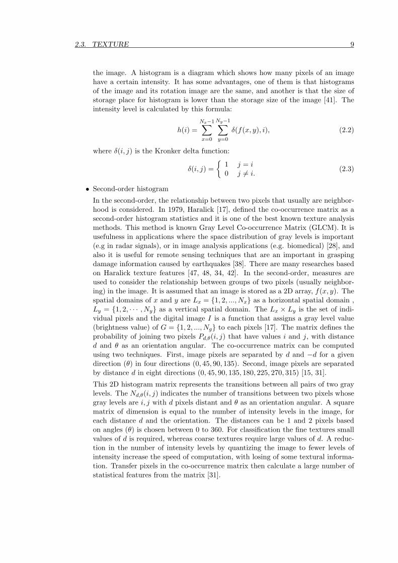
In the second-order, the relationship between two pixels that usually are neighbor-hood is considered. In 1979, Haralick [17], defined the co-occurrence matrix as asecond-order histogram statistics and it is one of the best known texture analysismethods. This method is known Gray Level Co-occurrence Matrix (GLCM). It isusefulness in applications where the space distribution of gray levels is important(e.g in radar signals), or in image analysis applications (e.g. biomedical) [28], andalso it is useful for remote sensing techniques that are an important in graspingdamage information caused by earthquakes [38]. There are many researches basedon Haralick texture features [47, 48, 34, 42]. In the second-order, measures areused to consider the relationship between groups of two pixels (usually neighbor-ing) in the image. It is assumed that an image is stored as a 2D array, f(x, y). Thespatial domains of x and y are Lx = {1, 2, ..., Nx} as a horizontal spatial domain ,Ly = {1, 2, · · · , Ny} as a vertical spatial domain. The Lx × Ly is the set of indi-vidual pixels and the digital image I is a function that assigns a gray level value(brightness value) of G = {1, 2, ..., Ng} to each pixels [17]. The matrix defines theprobability of joining two pixels Pd,θ(i, j) that have values i and j, with distanced and θ as an orientation angular. The co-occurrence matrix can be computedusing two techniques. First, image pixels are separated by d and −d for a givendirection (θ) in four directions (0, 45, 90, 135). Second, image pixels are separatedby distance d in eight directions (0, 45, 90, 135, 180, 225, 270, 315) [15, 31].

This 2D histogram matrix represents the transitions between all pairs of two graylevels. The Nd,θ(i, j) indicates the number of transitions between two pixels whosegray levels are i, j with d pixels distant and θ as an orientation angular. A squarematrix of dimension is equal to the number of intensity levels in the image, foreach distance d and the orientation. The distances can be 1 and 2 pixels basedon angles (θ) is chosen between 0 to 360. For classification the fine textures smallvalues of d is required, whereas coarse textures require large values of d. A reduc-tion in the number of intensity levels by quantizing the image to fewer levels ofintensity increase the speed of computation, with losing of some textural informa-tion. Transfer pixels in the co-occurrence matrix then calculate a large number ofstatistical features from the matrix [31].


• Higher order: In these methods the relationships between three or more pixels areconsidered.

2.3.4.3 Model-Based Methods

Model based texture analysis such as Fractal model, and Markov are based on the con-struction of an image that can be used for describing texture and synthesizing it [44].These methods describe an image as a probability models or as a linear combination ofa set of basic functions [48].

The Fractal model is useful for modeling certain natural textures that have a sta-tistical quality of roughness at different scales [44], and also for texture analysis anddiscrimination. This method has a weakness in orientation selectivity and is not usefulfor describing local image structures. Pixel-based models view an image as a collectionof pixels, whereas region-based models view an image as a set of sub patterns. Thereare different types of models based on the different neighborhood systems and noisesources. These types are one-dimensional time-series models, Auto Regressive (AR),Moving Average (MA), and Auto Regressive Moving Average (ARMA). Random fieldmodels analyze spatial variations in two dimensions, global random, and local random.Global random field models treat the entire image as a realization of a random field, andlocal random field models assume relationships of intensities in small neighborhoods. Awidely used class of local random field models are Markov models, where the conditionalprobability of the intensity of a given pixel depends only on the intensities of the pixelsin its neighborhood (the so-called Markov neighbors) [35, 31].

2.3.4.4 Transform Domain Methods

Transform methods, such as Fourier, Gabor, and wavelet transforms represent an imagein a space whose co-ordinate system has an interpretation that is closely related to thecharacteristics of a texture (such as frequency or size). They analyze the frequencycontent of the image. Methods based on Fourier transforms have a weakness in a spatiallocalization so they do not perform well. Gabor filters provide means for better spatiallocalization but their usefulness is limited in practice because there is usually no singlefilter resolution where one can localize a spatial structure in natural textures [35, 31].These methods involve transforming original images by using filters and calculating theenergy of the transformed images. They are based on the process of the whole imagethat is not good for some applications which are based on one part of the input image.

• Multi Resolution Techniques

In these techniques the preservation of an image is based on a certain levels ofresolution or blurring. Moreover, it zooms in and out of the underlying texturestructure so the texture extraction is not affected by the size of the pixel neigh-borhood. The multi resolution algorithm has two steps. The first step involvesthe automatic extraction of the most discriminative texture features of the regionof interested. In the second step, a classification that automatically identifies thevarious tissues is created [40].

2.3. TEXTURE 11

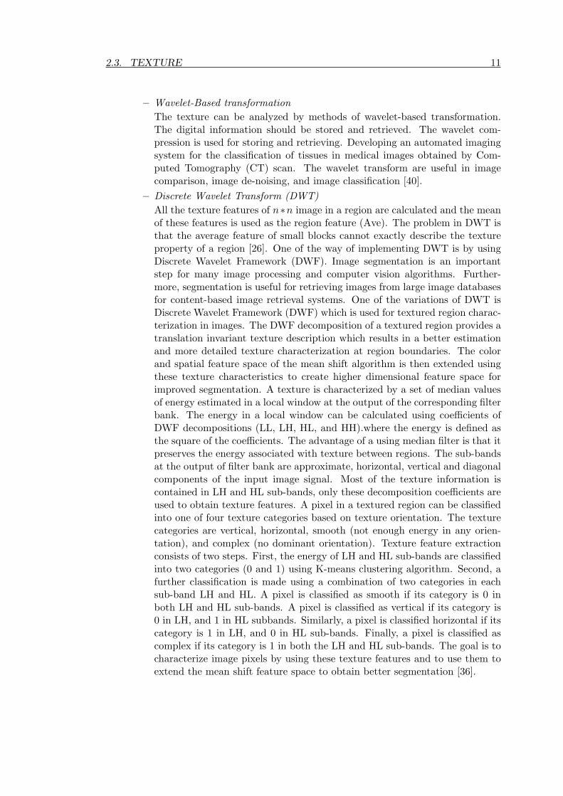
– Wavelet-Based transformationThe texture can be analyzed by methods of wavelet-based transformation.The digital information should be stored and retrieved. The wavelet com-pression is used for storing and retrieving. Developing an automated imagingsystem for the classification of tissues in medical images obtained by Com-puted Tomography (CT) scan. The wavelet transform are useful in imagecomparison, image de-noising, and image classification [40].

– Discrete Wavelet Transform (DWT)All the texture features of n∗n image in a region are calculated and the meanof these features is used as the region feature (Ave). The problem in DWT isthat the average feature of small blocks cannot exactly describe the textureproperty of a region [26]. One of the way of implementing DWT is by usingDiscrete Wavelet Framework (DWF). Image segmentation is an importantstep for many image processing and computer vision algorithms. Further-more, segmentation is useful for retrieving images from large image databasesfor content-based image retrieval systems. One of the variations of DWT isDiscrete Wavelet Framework (DWF) which is used for textured region charac-terization in images. The DWF decomposition of a textured region provides atranslation invariant texture description which results in a better estimationand more detailed texture characterization at region boundaries. The colorand spatial feature space of the mean shift algorithm is then extended usingthese texture characteristics to create higher dimensional feature space forimproved segmentation. A texture is characterized by a set of median valuesof energy estimated in a local window at the output of the corresponding filterbank. The energy in a local window can be calculated using coefficients ofDWF decompositions (LL, LH, HL, and HH).where the energy is defined asthe square of the coefficients. The advantage of a using median filter is that itpreserves the energy associated with texture between regions. The sub-bandsat the output of filter bank are approximate, horizontal, vertical and diagonalcomponents of the input image signal. Most of the texture information iscontained in LH and HL sub-bands, only these decomposition coefficients areused to obtain texture features. A pixel in a textured region can be classifiedinto one of four texture categories based on texture orientation. The texturecategories are vertical, horizontal, smooth (not enough energy in any orien-tation), and complex (no dominant orientation). Texture feature extractionconsists of two steps. First, the energy of LH and HL sub-bands are classifiedinto two categories (0 and 1) using K-means clustering algorithm. Second, afurther classification is made using a combination of two categories in eachsub-band LH and HL. A pixel is classified as smooth if its category is 0 inboth LH and HL sub-bands. A pixel is classified as vertical if its category is0 in LH, and 1 in HL subbands. Similarly, a pixel is classified horizontal if itscategory is 1 in LH, and 0 in HL sub-bands. Finally, a pixel is classified ascomplex if its category is 1 in both the LH and HL sub-bands. The goal is tocharacterize image pixels by using these texture features and to use them toextend the mean shift feature space to obtain better segmentation [36].


– Ridgelet-Based transformationThe Ridgelet transform derives information of an image that is based on mul-tiple radial directions not just in vertical and horizontal frequency domains.First, order statistics can be calculated on the directional then texture descrip-tors that can be used in the classification of texture are provided by applyinga 1D wavelet transform. In the Computed Tomography (CT) medical imagethe ridgelet-based algorithm is more useful than others [40].

• Fourier Transform

The Fourier Transform (FT) is in the signal processing methods and maps a signalinto its component frequencies or decomposes an image into its sine and cosinecomponents. It is useful in image compression, image filtering, etc. It is definedby either

f(k, l) =1N2

N−1∑i=0

N−1∑j=0

f(i, j)e−i2π( kiN

+ ljN

), (2.4)

where f(i, j) is the image in the spatial domain and K = 0, 1, ..., N − 1,

orFp(w) =

∫p(t)e−jwtdt, (2.5)

where w is the angular frequency and w = 2πf in radians/s and f is the frequencythat f = (1/t), t is the time, j is the complex variable and the p(t) is a continuoussignal in time, and e−jwt = cos(wt)j sin(wt) is the frequency components in x(t)[33].

– Discrete Fourier TransformThe DFT decomposes image into components of different frequencies and itscomplexity is O(N2). The weakness of DFT is that it is slow.

– Fast Fourier TransformThe Fast Fourier Transform has the same result with DFT but is much faster.It calculates one dimension of DFT. The complexity of FFT is O(N logN).

• Gabor

The Gabor Filters (GF) by Dennis Gabor [13] are linear filters that are used inimage analysis applications, such as texture classification, texture segmentation,image recognition, edge detection, image representation, etc. The GF extractinformation is based on time and frequency. These are useful for feature extractionfrom 2D images in texture analysis [35, 20]. The GF is defined according to thisformula:

g(x, y;λ, θ, ψ, σ, γ) = exp(− x2 + γ2y2

2σ2) cos(2π

x

λ+ ψ) (2.6)

where

x = x cos θ + y sin θ, (2.7)y = −x sin θ + y cos θ. (2.8)

2.3. TEXTURE 13

The λ represents the wavelength of the cosine, θ is the orientation, ψ is the phaseoffset, σ is the sigma of the Gaussian envelope, and γ is the spatial aspect ratio.

The Gabor features are calculated by the below formula and (x, y) is the spatialcoordinate, f as a frequency, and θ for orientation:

rξ(x, y; f, θ) = Ψ(x, y; f, θ) ∗ ξ(x, y)=

∫ ∫Ψ(x− xτ , y − yτ ; f,Θ)ξ(xτ , yτ ) dxτ dyτ .

(2.9)

Calculation texture features by Gabor has some difficulties, such as for determiningthe size of the Gabor filter window and the number of Gabor channels at the sameradial frequency [48].

Compared with the Gabor transform, the Wavelet transform feature has severaladvantages and are suitable for texture analysis [31]:

• varying the spatial resolution allows it to represent textures on the most suitablescale,

• There is a wide range of choices for the Wavelet function, so one is able to choosethe wavelet best suited to texture analysis in a specific application.

Furthermore, DWT is localized in both time and frequency and Fourier transform islocalized in frequency.

A texture description with Wavelet methods is done by filtering the image with a bankof filters, each filter having a specific frequency (and orientation), then texture featuresare extracted from the filtered images. For image with large dimension, often manyscales and orientations are needed [35]. These Wavelet advantages make it attractivefor texture segmentation.

2.3.5 Rules for Choosing Texture Extraction Algorithms

Each of these categories has some algorithms for texture feature extraction. To selectthese algorithms some characteristics should first be considered, these characteristics areas follow [35]:

• Illumination (gray-scale) invariance: The sensitivity of algorithm to change in grayscale. This aspect is an important when the lighting condition in industrial machinevision may be unstable.

• Rotation invariance: Does the texture of images change if we change the rotationof the images.

• Robustness in front of noise: The robustness ability of the algorithm is in the noisyenvironment which has an effect on input image.

• Computational Complexity: Many algorithms are computationally intensive, forexample in retrieval applications for large databases


• Generatively: Can the algorithm facilitate texture synthesis, i.e. by regeneratingthe texture that was captured using the algorithm.

• Popularity: Which of them are more popular and more practical.

• Easy to implement: The algorithm should be simple to implement.

Complexities of DWT, and GLCM are O(n), and fast Fourier transform and gabor areO(nlogn). I have chosen GLCM, based on its some characteristics as follows. Nowadays,the most common way to extract texture features is GLCM, it has been used in manyapplications, such as in content based image retrieval, biomedical, etc. Furthermore,GLCMs of an original image is the same with GLCMs of its rotation, hence it has arotation invariance character. In the section 3.8, we discussed about the comparisonbetween GLCM and other algorithms.

2.3.6 Statistical Algorithms for Texture Extraction

• First-order histogram based features: This method provides the 1D histogram ofan image based on its gray level. The histogram is simply a summery of thestatistical information about the image. The probable density (p(i)) of occurrenceof the intensity levels is calculated by dividing the values h(i) in the total numberof pixels in the Nx ×Ny image.

p(i) = h(i)/NxNy, i = {0, 1, ..., Ng − 1}. (2.10)

The histogram defines the characteristics of the image, for example, a narrowlydistributed histogram indicated the low-contrast image. A bimodal histogram oftensuggests that the image contained an object with a narrow intensity range againsta background of differing intensity [31].

The features that can be extracted are:

– Mean: The mean defines the average level of intensity of the image or texture

µ =Ng−1∑i=0

ip(i). (2.11)

– Variance: Which defines the variation of intensity around the mean

σ2 =Ng−1∑i=0

(i− µ)2p(i). (2.12)

– Skewness: It defines the symmetry.

µ3 = σ−3

Ng−1∑i=0

(i− µ)3p(i). (2.13)

2.3. TEXTURE 15

Skewness =

µ3 < 0 → Histogram is below the meanµ3 = 0 → Histogram is symmetrical to the meanµ3 > 0 → Histogram is above the mean

(2.14)

– Kurtosis: This is a measure of the flatness of the histogram

µ4 = σ−4

Ng−1∑i=0

((i− µ)4p(i))− 3. (2.15)

– Energy: That returns the sum of squared elements

E =Ng−1∑i=0

[p(i)]2. (2.16)

– Entropy:

H = −Ng−1∑i=0

p(i) log2[p(i)]. (2.17)

The other features which can be archived of the histogram are the maximum,minimum, median, and the range. The information of this histogram is used asfeatures for texture segmentation. The module that a measurement of histogram’sinformation is calculated by:

INyH(x, y) =Ng−1∑i=0

h(i)−Nx/G√h(i)[1− p(i)] +Nx/Ng(1− 1/Ng)

. (2.18)

The result of this technique is simple but texture cannot be completely charac-terized. This method is not useful for a large class of texture [31], and the otherweakness of this method is that the histogram of two different images that havethe same gray value for different pixels are equals. The complexity of this methodfor the Nx ×Ny image is O(Nx ∗Ny).

Example 3.1: Figure 2.5 shows two gray level matrix of size 5 × 5 and theirhistograms. Although, images are not same but their histograms is the same.That is a limitation of technique.

• Gray-Level Co-occurrence matrix

The Gray-Level Co-occurrence Matrix (GLCM) is based on the extraction of agray-scale image. It considers the relationship between two neighboring pixels, thefirst pixel is known as a reference and the second is known as a neighbor pixel [19].The GLCM is a square matrix with Ng dimension, where Ng equals the number ofgray levels in the image. Each element of the matrix is the number of occurrenceof the pair of pixel with value i and a pixels with value j which are at distanced [6, 28, 12].

The measuring of texture involves the following steps:


Figure 2.5: Example of first-order methods.

– Make the GLCM symmetrical

– Calculate the probability of each combination, the probability is calculated:

P(i,j,d,θ0) = #{((k, l), (m,n)) ∈ (Lr × Lc)× (Lr × Lc)|(k −m), (l − n) ∈ {−d, 0, d}|I(k, l) = i, I(m,n) = j, | 6 ((k, l), (m,n)) = θ}

(2.19)And p(i, j) is the element (i, j)th of the normalized co-occurrence matrix

pd,θ(i, j) =P(i,j,d,θ0)∑Ng

i=1

∑Ng

j=1 P(i,j,d,θ0)

(2.20)

If the co-occurrence matrix is symmetric then p(i, j) = (p(i, j) + p(i, j)T )/2that T indicates the transpose matrix and θ will be 0, 45, 90 and 135 [4].

– Calculated the texture features.

Haralick et al [17] defined 14 texture features, these features contain the in-formation about the image such as homogeneity, contrast, the complexity ofthe image, and etc. They are used in many applications such as biologicalapplications and image retrieval.

This adjacency can occur in four directions based on the angle, horizontal, vertical,right diagonal, and left diagonal. Figure 2.6 shows these directions.

2.3. TEXTURE 17

Figure 2.6: Diagram of angles, the Haralick texture features are calculated in each ofthese directions.

The following equations are needed for calculating Haralick texture feature.

px(i) =Ng∑j=1

pd,θ(i, j), (2.21a)

py(j) =Ng∑i=1

pd,θ(i, j), (2.21b)

px+y(k) =Ng∑i=1

Ng∑j=0

pd,θ(i, j), k = {2, 3, ..., 2Ng}, k = i+ j, (2.21c)

px−y(k) =Ng∑i=1

Ng∑j=0

pd,θ(i, j), k = {0, 1, ..., Ng}, k = |i− j|. (2.21d)

Haralick Texture Features:

With this method, 14 texture features are taken for each image. The features areas follows:

1. Angular Second Moment (ASM)ASM also known as uniformity or energy, measures the image homogeneity.ASM is high when pixels are very similar.

f1 =Ng∑i=1

Ng∑j=1

pd,θ(i, j)2. (2.22)


2. Contrast (CON)Contrast is a measure of intensity or gray-level variations between the refer-ence pixel and its neighbor. The visual perception is the difference in appear-ance of two or more parts of a field seen simultaneously or successively.

f2 =∑Ng−1

n=0 n2{∑Ng

i=1

∑Ng

j=1 pd,θ(i, j)}|i− j| = n.

(2.23)

3. Correlation (COR)Correlation calculates the linear dependency of the gray level values in theco-occurrence matrix [29]. It shows how the reference pixel is related to itsneighbor.

f3 =

∑Ng

i=1

∑Ng

j=1(ij)pd,θ(i, j)− µxµyσxσy

(2.24)

Where:µx, µy, σx, and σy are the means and standard deviations of px and py.

4. Sum of Squares: VarianceThis is a measure of gray tone variance.

f4 =Ng∑i=1

Ng∑j=1

(i− µ)2pd,θ(i, j). (2.25)

5. Inverse Difference Moment (IDM)IDM also sometimes called homogeneity, measures the local homogeneity of adigital image. IDM returns the measures of the closeness of the distributionof the GLCM elements to the GLCM diagonal.

f5 =Ng∑i=1

Ng∑j=1

11 + (i− j)2

pd,θ(i, j) (2.26)

6. Sum Average (mean)

f6 =2Ng∑i=2

ipx+y(i) (2.27)

2.3. TEXTURE 19

7. Sum Variance

f7 =2Ng∑i=2

(i− f8)2px+y(i) (2.28)

8. Sum Entropy

f8 = −2Ng∑i=2

px+y(i) log px+y(i) (2.29)

If the probability equals zero then the log(0) is not defined. To prevent thisproblem, it is recommended to use log(p + ε) that ε is an arbitrarily smallpositive constant, instead of log(p).

9. Entropy (ENT)Entropy shows the amount of information of the image that are needed forimage compression.

f9 = −Ng∑i=1

Ng∑j=1

pd,θ(i, j) log(pd,θ(i, j)) (2.30)

The high entropy image has a great contrast from one pixel to the itsneighbor and cannot be compressed as a low entropy image which has a lowcontrast (a lot of amount of pixels have the same or similar value) [6].

10. Difference Variance

f10 = variance of px−y (2.31)

11. Difference Entropy

f11 = −Ng−1∑i=0

px−y(i) log px−y(i) (2.32)


12. Information Measures of Correlation 1

f12 =HXY −HXY 1max (HX,HY )

(2.33)

13. Information Measures of Correlation 2

f13 = (1− exp[−2.0(HXY@−HXY )])1/2 (2.34)

where:

HXY = −Ng∑i=1

Ng∑j=1

pd,θ(i, j) log(pd,θ(i, j)) (2.35)

HX and HY are entropies of px and py

HXY 1 = −Ng∑i=1

Ng∑j=1

pd,θ(i, j) log (px(i)py(j)) (2.36)

HXY 2 = −Ng∑i=1

Ng∑j=1

px(i)py(j) log px(i)py(j) (2.37)

14. Maximal Correlation Coefficient

f14 = (Second largest eigenvalue of Q)1/2 (2.38)

where

Q(i, j) =∑k

pd,θ(i, k)pd,θ(j, k)px(i)py(k)

(2.39)

The variance is a measure of the dispersion of the values around the mean, it issimilar to the entropy. It is calculated by these formulas [15]: The complexity ofHaralick for an N ×N image is O(N2).

Example 3.2: A 4× 4 image with four gray level values 0− 3 is assumed.

The image is normalized as follows.

PH =

0.125 0.125 0.042 0.0420.042 0.042 0.083 0.0830.083 0.083 0.000 0.0000.000 0.000 0.125 0.125

.

2.3. TEXTURE 21

Figure 2.7: An image of size 4× 4.

Figure 2.8: Gray tone color

The mean is calculated as follows.

1 ∗ (0.125 + 0.125)+ 2 ∗ (0.042 + 0.042 + 0.083 + 0.083)+ 3 ∗ (0.083 + 0.083)+ 4 ∗ (0.125 + 0.125)= 1.332

(2.40)

For extracting texture features first the GLCM is calculated. Table 2.1 depictsthe construction of the GLCM for this example. Each element (i, j) of the matrixshows the total number of times that two gray tones of element i and j is occurredbased on a function of angle adjacent to each other.

The boundary of distance is calculated:

d((k, l), (m,n)) = max{|k - m|, |l - n|}.

The GLCM and Haralick features can be calculated using two techniques. In thefirst technique, the GLCM and Haralick features are calculated for each directionindividually, and then textures features of the input image are calculated based onthe features of each direction. In the second technique, the GLCM and featuresare calculated for all of directions at the same time.

In the first approach, the GLCM and texture features are calculated for eachdirection by assuming that distance (d) is equal to 1.

– Horizontal GLCM ( θ = 0◦)


i, j 1 2 3 41 #(0, 0) #(0, 1) #(0, 2) #(0, 3)2 #(1, 0) #(1, 1) #(1, 2) #(1, 3)3 #(2, 0) #(2, 1) #(2, 2) #(2, 3)4 #(3, 0) #(3, 1) #(3, 2) #(3, 3)

Table 2.1: Construction of co-occurrence matrix.

Figure 2.9: The symmetrical horizontal GLCM.

{k - m = 0,|l - n | = d.

∗ Symmetrical Horizontal GLCM:Each element of the GLCM, p(i, j), is a number of times that two pixelswith gray-tone i, and j are neighborhood in distance d, and directionsθ. Figure 2.9 shows how the symmetrical horizontal GLCM is calculated.The value in (0, 0) is the number of times that two pixels with gray-tone0 are neighborhood.

PH =

12 1 0 21 8 1 00 1 12 22 0 2 16

.

∗ Normalized Symmetrical Horizontal GLCM:The Normalization of GLCM: Each element of GLCM contains a proba-bility that is the value of each element divided by the total value of all ofthem. The total gray-value is 24.

PH =

0.2 0.017 0.000 0.033

0.017 0.133 0.017 0.0000.000 0.017 0.2 0.0330.033 0.000 0.033 0.267

.

2.3. TEXTURE 23

The ASM is: The ASM is 0.175.The mean is:

1 ∗ (0.2 + 0.017 + 0.033)+ 2 ∗ (0.017 + 0.133 + 0.017)+ 3 ∗ (0.017 + 0.2 + 0.033)+ 4 ∗ (0.033 + 0.033 + 0.267)= 3.338

(2.41)

– Right Diagonal GLCM (θ = 45◦){k - m = d, -d,|l - n | = -d, d.

∗ Symmetrical GLCM:

PH =

6 4 0 34 2 4 00 4 6 33 0 3 8

.

∗ Normalized Symmetrical Left Diagonal GLCM:The total gray-value is 18.

NPLD =

0.12 0.08 0.000 0.060.08 0.04 0.08 0.0000.000 0.08 0.12 0.060.06 0.000 0.06 0.16

.

The ASM is:0.122 + 0.082 + 0.0002 + 0.062

+ 0.082 + 0.042 + 0.082 + 0.0002

+ 0.0002 + 0.082 + 0.122 + 0.062

+ 0.062 + 0.0002 + 0.062 + 0.162

= 0.096

(2.42)

The mean is:1 ∗ (0.12 + 0.08 + 0.00 + 0.06)

+ 2 ∗ (0.08 + 0.04 + 0.08 + 0.00)+ 3 ∗ (0.00 + 0.08 + 0.12 + 0.06)+ 4 ∗ (0.06 + 0.00 + 0.06 + 0.16)= 3.12

(2.43)

– Vertical GLCM (θ = 90◦){k - m = d, -d,|l - n | = -d, d.


∗ Symmetrical Vertical GLCM:

NPLD =

0.12 0.08 0.000 0.060.08 0.04 0.08 0.0000.000 0.08 0.12 0.060.06 0.000 0.06 0.16

.

PV =

6 6 0 36 0 6 00 6 6 33 0 3 12

.

∗ Normalized Symmetrical Vertical GLCM:The total gray-value is 24.

NPV =

0.1 0.1 0.00 0.050.1 0.00 0.1 0.000.00 0.1 0.1 0.050.05 0.00 0.05 0.2

.

The ASM is:0.12 + 0.12 + 0.002 + 0.052

+ 0.12 + 0.002 + 0.12 + 0.002

+ 0.002 + 0.12 + 0.12 + 0.052

+ 0.052 + 0.002 + 0.052 + 0.22

= 0.11

(2.44)

The mean is:1 ∗ (0.1 + 0.1 + 0.00 + 0.05)

+ 2 ∗ (0.1 + 0.00 + 0.1 + 0.00)+ 3 ∗ (0.00 + 0.1 + 0.1 + 0.05)+ 4 ∗ (0.05 + 0.00 + 0.05 + 0.2)= 3.2

(2.45)

– Left Diagonal GLCM (θ = 135◦){k - m = d, -d,|l - n | = -d, d.

∗ Symmetrical GLCM:

PLD =

4 4 1 34 0 4 21 4 4 33 2 3 8

.

2.3. TEXTURE 25

∗ Normalized Symmetrical Left Diagonal GLCM:The total gray-value is 18.

PLD =

0.08 0.08 0.02 0.060.08 0.00 0.08 0.040.02 0.08 0.08 0.060.06 0.04 0.06 0.16

.

The ASM is:0.082 + 0.082 + 0.022 + 0.062

+ 0.082 + 0.002 + 0.082 + 0.042

+ 0.022 + 0.082 + 0.082 + 0.062

+ 0.062 + 0.042 + 0.062 + 0.162

= 0.082

(2.46)

The mean is:1 ∗ (0.08 + 0.08 + 0.02 + 0.06)

+ 2 ∗ (0.08 + 0.00 + 0.08 + 0.04)+ 3 ∗ (0.02 + 0.08 + 0.08 + 0.06)+ 4 ∗ (0.06 + 0.04 + 0.06 + 0.16)= 3.28

(2.47)

In the second technique the GLCM is calculated as follows by assuming d equals 1is that:

– Symmetrical GLCM: The GLCM is calculated for four directions

PT =

28 9 1 1115 10 15 21 15 28 1111 2 11 44

.

– Normalized Symmetrical Left Diagonal GLCM: The total gray-valueis 76.

PT =

0.127 0.068 0.005 0.050.068 0.045 0.068 0.0090.005 0.068 0.127 0.050.05 0.009 0.05 0.2

.

The ASM is: The ASM is 0.103 that near sum of all ASMs values of eachdirections.The mean is: The mean is 3.234, with comparing this mean and the averageof means for all angle, we can conclude that the mean of the input image isthe average of means each directions.


Figure 2.10: 4× 4 rotated image.

Example 3.3 : One of the characters of GLCM is that with rotation the inputimage, its GLCM does not change. If the image is rotated, the gray-scale view ofimage is, Figure 2.10 shows the gray level of this image.

The GLCM matrix is:

– GLCM:

PH =

28 15 1 1115 10 15 21 15 28 1111 2 11 44

.

– Normalized GLCM:

PH =

0.127 0.068 0.005 0.050.068 0.045 0.068 0.0090.005 0.068 0.127 0.050.05 0.009 0.05 0.2

.

The ASM is: The ASM is 0.103.

The mean is: The mean is 3.234

We can conclude the GLCM and texture features of the input image and its rotatedimage are the same.

2.3.7 Comparison between Co-occurrence and others Algorithms

A vast body of work on comparing texture features algorithms exists. Weszka et al [47]applied texture features of Haralick and Fourier on photographs of nine Terrain types(Lake, Marsh, Orchard, Railroad, Scrub, Suburb, Swamp, Urban, and Woods) for textureclassification, their results shows haralick features have better performance than Fourier.Ohaniand et al [34] compared performance of features of Markov, Gabor, Fractal, andGLCM in recognizing classes of visual textures. They concluded GLCM has a betterperformance than others. du Buf et al [48] compared features of different algorithmsfor image segmentation and their results show GLCM has a better performance. On

2.3. TEXTURE 27

the other hand, GLCM has some weakness. In feature based segmentation application,the classification is performed in the feature space constructed by entropy, correlation,energy, contrast and homogeneity feature [18]. Furthermore, for small image size, andgray-tone values, GLCM is computed as a spareness. In total, GLCM is suitable forgray-tone values more than 32.

2.3.8 Computational Overhead of Co-occurrence Processing

The overall computational complexity time is computation time of calculation theGLCM, normalization of the GLCM, and calculation of texture features. Most of thetime is spent for calculation of GLCM. There are different methods for decreasing theGLCM time consumption. In one method the image is represented by four or five bitsinstead of eight bits that makes to reduce the size of GLCM but it makes to removesome information about the image. Another method is that to reduce the size of GLCMby storing just non-zero values. Clausi and Jernigant [9] describe the gray Level Co-occurrence Linked List (GLCLL). In GLCLL just non-zero values of GLCM are storedin a linked list, and each linked list node contains the two co-occuring gray-values, theco-occurrence probability of these two pair gray-values, and a link to the next node.when a new pair (i, j) comes, first there is a search for finding i, if it is found then thereis a search for j. If there is a (i, j) in the list, their probability is increased, else thenew node is added to the list. The GLCLL increases the calculation time. In 2001,Clausi and ZhaoThe [10] Gray Level Co-occurrence Hybrid Structure (GLCHS) that isbased on an integrated hash table and linked list. Each node of the linked list includestwo integer elements to store the gray-value pairs and two pointers to the previous andthe next node. In the hash table, one element stores the probability of the GLCM andanother stores the linked list pointer. Access to the hash table is provided by using (i, j).Each entry in the hash table has a pointer. A null pointer indicates that a particularco-occurring pair (i, j) does not have a representative node. Each new node inserted atthe end of the linked list and its gray level values would be set. If the pointer is not null,then the probability of the existing node on the linked list is increased. The hash tableallows rapid access to an (i, j). GLCHS is faster than GLCLL, and is useful for largeimage but it results increased a complexity of implementation due to a two dimensionalhash table with longer linked list [10, 9]. In 2002, Clausi and Zhao [11] present newmatrix of GLCM, the gray Integrated Algorithm (GLCIA) based on the combinationbetween the gray Level Co-occurrence Hybrid Structure (GLCHS) and the gray LevelCo-occurrence Hybrid Histogram (GLCHH).

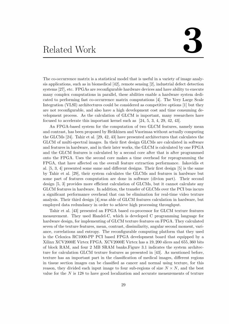
Related Work 3The co-occurrence matrix is a statistical model that is useful in a variety of image analy-sis applications, such as in biomedical [42], remote sensing [2], industrial defect detectionsystems [27], etc. FPGAs are reconfigurable hardware devices and have ability to executemany complex computations in parallel, these abilities enable a hardware system dedi-cated to performing fast co-occurrence matrix computations [4]. The Very Large ScaleIntegration (VLSI) architectures could be considered as competitive options [1] but theyare not reconfigurable, and also have a high development cost and time consuming de-velopment process. As the calculation of GLCM is important, many researchers havefocused to accelerate this important kernel such as [24, 5, 3, 4, 29, 42, 43].

An FPGA-based system for the computation of two GLCM features, namely meanand contrast, has been proposed by Heikkinen and Vuorimaa without actually computingthe GLCMs [24]. Tahir et al. [29, 42, 43] have presented architectures that calculates theGLCM of multi-spectral images. In their first design GLCMs are calculated in softwareand features in hardware, and in their later works, the GLCM is calculated by one FPGAand the GLCM features is calculated by a second core after that is after programmedonto the FPGA. Uses the second core makes a time overhead for reprogramming theFPGA, that have affected on the overall feature extraction performance. Iakovidis etal. [5, 3, 4] presented some same and different designs. Their first design [5] is the sameby Tahir et al. [29], their system calculates the GLCMs and features in hardware butsome part of features computation are done in software (divion part). Their seconddesign [5, 3] provides more efficient calculation of GLCMs, but it cannot calculate anyGLCM features in hardware. In addition, the transfer of GLCMs over the PCI bus incursa significant performance overhead that can be elimination for real-time video textureanalysis. Their third design [4],was able of GLCM features calculation in hardware, butemployed data redundancy in order to achieve high processing throughput.

Tahir et al. [43] presented an FPGA based co-processor for GLCM texture featuresmeasurement. They used Handel-C, which is developed C programming language forhardware design, for implementing of GLCM texture features on FPGA. They calculatedseven of the texture features, mean, contrast, dissimilarity, angular second moment, vari-ance, correlations and entropy. The reconfigurable computing platform that they usedis the Celoxica RC1000-PP PCI based FPGA development board that equipped by aXilinx XCV2000E Virtex FPGA. XCV2000E Virtex has a 19, 200 slices and 655, 360 bitsof block RAM, and four 2 MB SRAM banks.Figure 3.1 indicates the system architec-ture for calculation GLCM texture features as presented in [43]. As mentioned before,texture has an important part in the classification of medical images, different regionsin tissue section images can be classified as cancer and normal using texture, for thisreason, they divided each input image to four sub-regions of size N × N , and the bestvalue for the N is 128 to have good localization and accurate measurements of texture

29

30 CHAPTER 3. RELATED WORK

Figure 3.1: System architecture for calculation GLCM texture features [43].

features [37]. The GLCM for each sub-region is calculated for 4 distances d = {1, 2, 3, 4}and 4 directions θ = 0, 45, 90, 135 at host, then all results are loaded into 4 differentSRAM banks in Celoxica RC1000-PP PCI. FPGA reads the GLCM results from SRAMbanks and calculates features. Features are stored into bank0 of SRAM for image pro-cessing (segmentation, classification, and etc). THe input image is stored into memorybank 0 for acceding to the reference pixels and the same sub-region are stored into theother 3 banks of SRAM to access 4 neighbors pixels of reference pixel then 16 GLCMare calculated in parallel for reference pixel. Each element of GLCM is updates thenumber of occurrence of pixel. Then all GLCM are normalized in parallel and the resultof calculation features are stored into bank 0 of SRAM for further image processing suchas image classification, image segmentation, and etc. These calculations are done foreach pixel of the input image. After the calculation for all pixels in one sub-region isdone, the next sub-region is loaded and these processes are repeated. Then seven of Har-alick texture features are calculated. Calculation of features has two steps, in the firststep, mean, contrast, dissimilarity, and entropy are calculated, and in the second stepangular second moment, variance, and correlation depend upon the value of mean arecalculated. Figure 3.2 shows the block diagram of extraction Haralick features. Thereare five Processing Units (PUs), the first four PU include adders and multipliers, andcalculate seven texture features at distance d for different directions θ, PEs are executedin parallel. The final PU includes adders and shift registers and calculates the average ofeach feature that is calculated at distance d for different angles θ, and results are storedin SRAM bank 0. These processes will repeat for another distance. The feature calcula-tion operation has two steps, in the first step, mean, contrast, entropy, and dissimilarityare calculated into four different Processing Elements (PEs). PEs contain multipliersand adders that execute in parallel. Furthermore, for increasing the computation speed,(i − j) and (i − j)2 are pre-computed and stored in ROM, and also log tables in blockRAM are used for the calculation of the log function in the entropy. In the second step,angular second moment, variance, and correlation are calculated. In the computation,the real number arithmetic and fixed point number are used.

The Handel-C is a high level language for implementing algorithms in hardware, ithas a parallel composition keyword (par) to allow statement in a block to be executed inparallel [29], the PEs are executed in parallel by using this keyword. The output from

31

Figure 3.2: Block diagram of extraction Haralick features [43].

Handel-C is used to create the configuration data for the FPGA Celoxica DK1 is usedto compiles the C program into synchronous hardware [22]. Based on their experiment,the performance of implementation on FPGA is 7 times faster than implementation onPentium 4 with 2400 MHz clock, even the PC has a clock speed more 50 times fasterthan clock speed of FPGA [29]. In A 16 bit integer for the GLCM, a 32 bit floating pointfor the normalization of the GLCM are used, and in FPGA a 14 bit fixed point numberfor the GLCM and 24, 20, 16 bit fixed point numbers for the normalization of GLCM.Their results show that the performance of FPGA is approximately 9 times faster thanPentium 4, and also the speed of FPGA are independent of the image size. FPGA ontheir design executes one sub-region at a time and the rest of sub-regions are looped.They used pipelining and parallelism for implementation. A later work by Tahir et al.[42] presents an FPGA based coprocessor for GLCM and Haralick texture features andtheir applications in prostate cancer classification. Figure 3.3 indicates their algorithms.Their target device is the Celoxica RC1000-PP PCI based FPGA development boardthat equipped by a Xilinx XCV2000E Virtex FPGA. XCV2000E Virtex has a 19, 200slices and 655, 360 bits of block RAM, and four banks of SRAM with 2MB for eachof them. The system model of their design is shown in Figure 3.4. In contrast withthere’s another research [29], they calculate GLCM and texture features in the FPGA.The host is a PC-Pentium 4, and works as a Control Unit (CU), which loads differentinput images for each stage of the external memory of the FPGA. The input image isdivided into sub-regions of size 128 ∗ 128, and GLCMs are calculated for four distanced = {1, 2, 3, 4} and four directions θ = 0, 45, 90, 135 at the same time. In total, theycalculate 16 GLCMs. The sub-region with N ∗ N is stored into four SRAM’s bank toread four neighbor pixels of reference pixel in parallel. The block diagram of calculationGLCM is shown in Figure 3.5. The process starts with reading the first pixel of each


Figure 3.3: Algorithm for the classification of prostate tissue cancer [4].

Figure 3.4: System model [4].

bank; these pixels are known as reference pixel, then their four neighbors are read in 4clock cycles, after that the memory address of all 16 GLCMs are calculated in paralleland the number of occurrences of pixels in co-occurrence matrix is updated, the processis repeated for all of the image pixels [42]. After calculated all 16 GLCMs in parallel,these matrixes are normalized in parallel too. The final results of normalization arestored into SRAM of the FPGA. Then the calculation and normalization are repeatedfor other sub-regions. The rest of their research for calculation texture features are thesame with their pervious jobs [29]. Their results show that the performance of FPGAis 5 times faster than the Pentium 4PC, the reason is related to calculate GLCMs inparallel, and the computation time is independently of size of the input image. Eachinput image is divided into sub-regions with size N ∗N , that the best value for the N is128. FPGA executes one sub-region at the time, and others are in the loop.

Iakovidis et al. [5](2004) presented an FPGA based architecture for real time im-age feature extraction using GLCM analysis in 2004. They implemented their hardwaremodule on Xilinx Virtex-E V2000 FPGA. Their design calculates GLCMs and GLCM in-teger features in parallel, and their architecture is combination of hardware and softwareto raster scan input images with sliding windows and calculate 16 dimensional featurevectors consisting of 4 GLCM features for 4 directions. They calculate four of texturefeatures, namely, angular second moment, correlations, inverse difference moment, andentropy. Their architecture has two steps, a preprocessing stage and the feature extrac-tion block. Figure 3.6 is an overview of the architecture.

In the preprocessing steps, the input image is prepared to be processed by the feature

33

Figure 3.5: Block diagram of calculation GLCM on FPGA [4].

extraction block. For preparation, the input image is convert to an array A, each elementof the array is presented by a = {a0a1a2a3a4}, (5 integers) that is related to each pixel,a0 is the gray-value of the reference and other are the gray-values of reference pixel infour directions. They assumed, the gray-value is up to 64 that can be presented by 6bits so each element is shown by 30 bits and read in 1 clk. The second step is a combi-nation of hardware and software for calculation GLCM features, the feature extractionblock includes hardware and software module. The hardware module is implementedon a Xilinx Virtex-E V2000 FPGA and the FPGA is hosted by the Celoxica RC1000card. The host preprocesses the input image and presents each pixel as a one elementof the array A and loads the result into one of the four memory banks on the card, theFPGA calculates the feature vectors and stores them into in another memory bank [5].


Figure 3.6: Overview of the FPGA architecture [5].

The FPGA architecture consists of Control Unit (CU), Memory Controller, GLCM Cal-culation Unit (GLCMCU), and Feature Calculation Unit. The CU generates signalsthat synchronize the other units to coordinate the FPGA’s functionality. The memorycontroller handles the transactions from and to the on-card memory. The GLCMCUreceives pairs of gray-value of reference pixel and one of its neighbors as input. Theinput of feature extraction unit is a GLCM generated by each GLCMU and its output,that is a vector V = {V1, V2, V3, V4, Vs} is stored on the on-card memory. As mentionedbefore, they consider to four of texture features, they replaced the integer operationsinstead of floating point operations to simplify the hardware implementation [5]:

1. Angular Second Moment (ASM)

f1 = (Ng∑i=1

Ng∑j=1

c2ij)/r2. (3.1)

2. Correlation (COR)

f2 = (r.N2g

Ng∑i=1

Ng∑j=1

i.j.c(ij)− r2).Ng − 1S

(3.2)

S =Ng∑k=1

(r − Cx(k))2 (3.3)

35

3. Inverse Difference Moment (IDM)

f3 = 2−30.

Ng∑i=1

Ng∑j=1

cij .IDMLUT [i− j] (3.4)

4. Entropy (ENT)

f4 = 2−26.

Ng∑i=1

Ng∑j=1

cij .(LOGLUT [cij ]− 226.logr) (3.5)

Where ci,j is the ijth 16-bit registerVectors are defined by these equations:

V1 =∑

c2ij , (3.6a)

V2 =∑

i.j.c(ij), (3.6b)

V3 =∑

cij .IDMLUT [i− j], (3.6c)

V4 =∑

cij .(logcij − logr), (3.6d)

VS =∑

(r − Cx(k))2. (3.6e)

The software module, reads the vectors V and converts the integer component of eachvector into 32-bit floating point values, and calculates the corresponding GLCM features.In this design, they use integer operations and also their input image has a limitationfor gray-values up 64 bit.

Iakovidis et al. [3](2006) presented a dedicated hardware system for the extractionof second-order statistical features from high-resolution images, they extracted four ofHaralick texture features, ASM, COR, IDM, and ENT. The input images can have aresolution from 512 × 512 to 2048 × 2048 pixels. They implemented their architectureon a Xilinx VirtexE-2000 FPGA and used integer arithmetic, a sparse co-occurrencematrix representation and a fast logarithm approximation to improve efficiency. Eachimage is divided into blocks of user-defined size and a feature vector is extracted for eachblock. Their system calculates a symmetric GLCM for four directions 0, 45, 90, 135 andfor distances so in total 16 GLCM are calculated, and four feature vectors on the sameFPGA core in parallel. There are CU, and CMCU, Vector Calculation Units (VCUs) intheir design. For each direction, one CMCU is used. They define Ng as 64 bits insteadof 32 bits that used in [4], and changed their hardware. These CMCUs are designed forachieving to the three objects, as follows,

• Small FPGA area utilization that makes just one core is used for calculation ofGLCM and four VCUs

• High throughout per clock cycle


Figure 3.7: Overview of the FPGA architecture [4].

• High frequency potential

They used a v = {v1, v2, v3, v4, v5} for calculating features. This design is suitable forhigh regulation video, analysis of the multiple video streams. Furthermore, by usingone core, there is no overhead by reprogramming cache core onto the FPGA. Eachpixel is represented by 25 bits so at each CLK 25 bits from each memory bank is readwhen in Tahir et al design each pixel is represented by 5 bits. By using set-associativearrays for each sparse GLCM, four vectors can be calculated in a single core. They justimplemented four features of Haralick [3].

Iakovidis et al. [4](2007) present a FPGA architecture for fast parallel computationarchitecture of co-occurrence matrices in high throughput image analysis applicationsthat performance is an important, and they extracted four of Haralick texture features,namely, ASM, COR, IDM, and ENT. Their target device is Xilinx Virtex XCV2000E-6FPGA. This architecture calculates a symmetric and sparseness co-occurrence matricesin four directions 0, 45, 90, 135 and for distances (16 GLCMs), and also four featurevectors on the same FPGA core in parallel. The input The input image is divided intoblocks of user-defined size and a feature vector is extracted for each block, each pixel ofthe image is presented by a vector a = {ap, a0, a45, a90, a135}, that ap is the grey-level ofthe reference pixel and others are the grey-levels of its neighboring. The architecture ofFPGA for GLCM shows in Figure 3.7. This architecture consists of a control unit, sixteenCo-occurrence Matrix Computation Units (CMCUs), and nmemory controllers that eachof them is for one memory bank. In parallel up to n input images of Ng grey-levels can beloaded in memory banks. They use one FPGA core for calculating GLCM and featuresso there in no overhead by reprogramming each core onto FPGA [4]. The Control Unit(CU) organizes all FPGA functions, creates synchronization signals for the memorycontrollers and the CMCUs, and communicates with the host, by exchanging controland status bytes, and request or release the rights of the memory banks. Each CMCUis used for calculating the co-occurrence matrix of an image for a different directionand distance [4]. Their results show the feasibility of real-time feature extraction forinput images of dimensions up to 2048x2048 pixels, where a performance of 32 imagesper second is achieved. This architecture calculates a symmetric and sparseness of theGLCMs to achieve improved processing times, and smaller, flexible area utilization

FPGA Implementation 4In this chapter, the proposed model for calculating GLCM is presented. The chapter isorganized as follows. The first section represent a description of FPGA, and comparisonbetween FPGA and ASIC. Section Section 4.1.1 presents the description of hardwaretargets. The function of design is described in section Section 4.2. The design was devel-oped in Very High Speed Integrated Circuits Hardware Description Language (VHDL),and three hardware targets are used for calculation of 16 GLCMs in four distance withfour angles. The common value for angles are 0o, 45o, 90o, 135o [29, 4, 42], and the valuesof distances are d = 1, 2, 3, 4. In last section, the results and their analysis are presented.

4.1 FPGA

Field Programmable Gate Array (FPGA) is a semiconductor device that can be pro-grammed by user after manufacturing and implemented by any logical functions thatan Application Specific Integrated Circuit (ASIC) could perform, these abilities proposeadvantages for many applications. FPGAs consist of various mixes of embedded SRAM,high-speed I/O, logic blocks, and routing. In particular, an FPGA has a programmablelogic components, which called logic blocks and a hierarchy of reconfigurable intercon-nects. Logic blocks consist of a Look-Up Table (LUT) for logical functions and memoryelements or blocks of memories, which may be simple flip-flop or more complete blocksof memory for storage [21]. Reconfigurable interconnects allow the logic blocks to bewired together.

4.1.1 FPGA vs ASIC

As opposed to ASICs, FPGAs can be programmed in several times based on design andmemory bits and logic gates. However, ASICs have high development cost and timeconsuming development procedure and just memory bits are controlled by user. On theother hand, FPGAs are slower than ASIC. The choice of whether to use of FPGA or ASICis based on design, the chip will need to be reprogrammed or not, and cost. Sometimes,first design is prototyped on FPGA and after find the stable design, is implemented onASIC. One of the applications that FPGAs are used is real time image processing thatneeds to be run in parallel. Image and video application need a wide area but basedon limitation in memory bandwidth, and confliction in resource (e.g. local and off-chipRAM), the input image is divided into equal parts and processing is done in multiplepipeline process.

37

38 CHAPTER 4. FPGA IMPLEMENTATION

4.2 Hardware Target

The hardware targets are Xilinx Virtex-XC2VP30, Virtex- XC4VfX60, and XC5VLX330.Virtex-XC2VP30 is characterized by 3424 CLBs providing 13, 696 slices, which each

CLB is 4 slices, and has 136 18 Kb True Dual-Port Bock RAM. Table 4.1 shows theavailable resources in virtex-XC2VP30. Each logic cell has one 4-input LUT, one FlipFlop (FF), and carry logic.

RocketlO PowerPC CLB (1 = 4 slices = 18 × 18 BitBlock SelectRAM+

Maximum

Device transceiver Processor Logic Cells max 128 bits) Multipler DCMs User

Blocks Blocks Slices Max DistrRAM(kb)

Blocks 18 Kb Blocks Max BlockRAM(kb)

I/O Pads

XC2VP30 8 2 30816 13696 428 136 136 2448 8 644

Table 4.1: Virtex-XC2VP30.

Virtex-XC4VfX60 conta 6320 CLBs providing 25, 280 slices, which each CLB is 4slices. Table 4.2 depicts the available resources in this virtex. Each CLB is 4 slices andoptimized by 64 bits, is means that at each cycle, 64 can be access.

DeviceConfigurable Logic Blocks (CLBs) Block RAM PowerPC Total Max

Array LogicSlices

Max XtremeDSP 18Kb Max Block DCMs PMCDs Processor Ethernet I/O User

Row ×Col Cells Distributed RAM (Kb) Slices Blocks RAM (Kb) Blocks MACs Banks I/O

XC4VfX60 128×52 56880 25280 395 128 232 41760 12 8 2 4 13 576

Table 4.2: Virtex-XC4VfX60.

DeviceConfigurable Logic Blocks (CLBs) Block RAM Blocks PowerPC Endpoint Max RocketlO Total Max

Array Virtex-5 Max DSP48E18 (Kb) 36 (Kb) Max (Kb)

CMTs Processor Block for Ethernet Transeiver I/O User

Row ×Col Slices Distributed RAM (Kb) Slices Blocks PCI Express MACs GTP GTX Banks I/O

XC5VLX330 240×108 51.840 3420 192 576 288 10368 6 N/A N/A N/A N/A N/A 33 1200

Table 4.3: Virtex-XC5VLX330.

Virtex-XC5VLX330 has a 6-input LUT, and 36Kb BRAM. The 4-input LUT has atruth table capacity for 16 different combinations but with 6-input LUT, the truth tableis increased to 64 different combinations. Table 4.3 depicts the available resources inVirtex- XC5VLX330. Comparison with other Virtex, it has more memory, low powerand higher speed than virtex4.

All three Virtexs have a true dual port BRAMs. Each port has an individual clock,enable, reset, write enable, address, data input, and data output lines. The advantageof dual port is that we can access to different address in BRAM at the same time forread and write operation.

4.3 Proposed Design

There are different ways to calculate GLCMs. In the simplest way, GLCMs are seriallycalculated. This way takes more time because each pixel should be compared with each

4.3. PROPOSED DESIGN 39

of its neighborhood pixels one by one. Another way is calculation 4 GLCMs in parallelfor four directions and one distance. In the third way, which has been implemented inthis thesis, GLCMs are calculated for four distances d = 1, 2, 3, 4 and four directions0o, 45o, 90o, 135o in parallel. This technique increases the throughput. These differentdistances and directions are depicted in Figure 4.1

Figure 4.1: Different distances with four different directions, which have been used tocalculate sixteen GLCMs.

The proposed design consists of three main parts. First, an image is divided intosub-regions. Second, each sub-region is loaded. Finally, sixteen GLCMs are computedfor loaded sub-region. The last two steps are repeated for all sub-regions. These stagesare depicted in Figure 4.2.

Figure 4.2: Proposed model.

The image sizes of 32× 32, 64× 64, and 128× 128 have been used in our implemen-tations. In our design, we used BRAMs for storing input image and calculated GLCMs.The number of BRAMs depend on the image size and the number of gray levels (Ng).We generated these BRAMs with core generator. These BRAMs are dual port. It ispossible that those BRAMs are defined either one port or dual ports. We defined twotypes of BRAMs, input BRAMs and output BRAMs. The input BRAMs are definedas a single port and input image is stored into them. If the size of the input imageis small then that image can be stored in a BRAM, while if the image is large it canbe stored in several BRAMs. Four BRAMs are also used for storing the neighboring


pixels at four distances and four directions. The output BRAMs are defined as dualport. The calculated GLCMs are stored in output BRAMs. The reason to define theseBRAMs as a dual port is that the calculated GLCMs are symmetrical. Hence, we needto write same value into different address at the same time. For example, for image size32 × 32 with Ng = 32, there are 25 BRAMs, one BRAM for storing the original image(sub-regions) that each pixel of the original image is known as a reference pixel, eightBRAMs that each of two BRAMs for storing neighboring pixels of each reference pixel atfour directions 0o, 45o, 90o, 135o with four distances d = 1, 2, 3, and 4, and 16 BRAMs isused to store 16 calculated GLCMs. The overview of the FPGA architecture with theseassumptions is depicted in Figure 4.3.

Figure 4.3: Overview of the input and output BRAMs for the image size 32 × 32 andNg = 32.

As this figure shows, five BRAMs are used as input BRAMs and sixteen BRAMs areused as output BRAMs. The first input BRAM has N ×N M -bit, where N ×N is thesize of the image and M is the number of bits to represent each pixel of image. In otherwords, Ng = 2M . Each BRAM of other input BRAMs has K 4 ×M -bit, where 2K isN ×N . This is because we have considered four neighboring pixels at each distance foreach reference pixel. The size of each output BRAM is 2M ×K-bit. Figure 4.4 depictsthe architecture of input BRAMs and output BRAMs.

Our design contains 17 Processing Unit (PU), one PU is used for reading a pixelfrom the input image, and other PU read its neighborhood and calculate GLCMs orload new value on output BRAMs. All these PU are run in parallel Figure 4.5 showsthe architecture of our design for reading a reference pixel and one of its neighboringfrom input BRAMS and loading data on output BRAM. These PUs work in parallel.In the first PU, a reference pixel is read from input BRAM0, each other PU read oneof the sixteen neighborhood of the reference pixel. For example, the second PU reads

4.4. RESULTS 41

Figure 4.4: Architectures of BRAMs for Ng = 32.

the pixel with d = 1 in directions 0o that located into last M bits of input BRAM1, andPU6 reads the pixel with d = 2 in directions 0o that is located into the third M bitsof BRAM1. With the value of gray tone of these pixels address for accessing to outputBRAMs are calculated, and data in this address are increased by one. As mentioned inpervious chapter there are two types of GLCM, symmetrical, and non-symmetrical. Inthis design, symmetrical GLCMs are calculated by generating output BRAMs as truedual port, so at the same time, the same value can be write into two different addresses.For example, if the gray tone value of reference pixel is known as a index i, and the graytone value of one of the neighborhood pixel is known as an index j, at the same timethe value in (i, j) and (j, i) will be increased.

4.4 Results

Experimental evaluation has been performed based on performance and area utilization.The proposed technique has been simulated on three target platforms, Virtex-XC2VP30,Virtex-XC4VfX60, and Virtex-XC5VLX330. The image sizes are 32 × 32, 64 × 64, and128× 128, with three Ng = 32, 64, 128 values.

The Processing Time (PT) can be calculated either by simulations or by theoretically.The PT is the multiplication of total execution cycles with the cycle period, when thesimulations are used. while, from the theoritically point of view, the PT is equal to themultiplications of clock period with the number of image pixels and the number of cyclesthat needed to process each image pixel (Np). PT = clock period x N x N x Np. whereN ×N is the dimension of an image.


Figure 4.5: Processing units.

The clock frequency is based on how a hardware design can be optimized. First, weexpected that clock period of the Virtex5 should be lower than others but it was not, itappeared that Virtex2 has the lowest clock period. The reason is that, we have a criticalpath for accessing to the Block RAMs. In different Virtex devices, this time is different.In general, the accessing time is related to the hardware design and the size of BlockRAM. With increasing a Block RAM size, the memory access times will be increased.In Virtex5, BRAM size is 36Kb, hence it takes longer time to read data from BRAMsthan other Virtex devices. Figure 4.6, Figure 4.7, and Figure 4.8 depict the obtainedclock period and frequency on different Virtex platform for different image size.

Figure 4.6: Frequency and clock period Ng = 32.

Based on the results for clock period, we computed processing times theoretically forour experiments. The achieved processing times for computation 16 GLCMs are depictedin Figure 4.9.

Based on our achievements, we can conclude, the variance in processing time is relatedto different frequencies of the different FPGA devices, and the design.

Figure 4.10 until Figure 4.12 show comparison graph of the processing time for dif-ferent image size with the same gray-tone values in different device.

4.4. RESULTS 43



Based on the above figures, The XC2VP30 has the lowest processing time in our de-sign. However, the number of BRAM available in XC2VP30 is less than other platforms,and it cannot supported an input image with the size 128× 128 and also for image withNg = 128. To deal with this limitation, we can make exception for the input image,and the data size of output BRAMs. In general, the output BRAMs data size is themaximum number of pairs (i, j) that is 2N , where N is image size. By make limitationfor the number of occurrence, we can have 128 × 128 with Ng = 64 or Ng = 128 asan input image for XC2VP30. For example, when the image size is 128 × 128, withNg = 128, the maximum number is 16384 that represents by 14-bits. In that case, forusing XC2VP30, we assumed the maximum number of occurrence is 29, hence data sizeof output BRAMs is 9 bits. Figure 4.13 shows the new result with this limitation for allVirtex devices.

Another conclusion is that, Vritex5-330 has a better throughput than XC4VFX60for a bigger image. The number of resources that used in Virtex5 is less than Virtex4and the processing time is better.

The area utilization of different implementations are depicted from Figures 4.14 toFigure 4.23.

We can make some conclusions regarding the results of the area utilization. One of theconclusion is that, implementation on Virtex-XC5VLX330 uses less resources comparedto the other Virtex devices, except the number of used slices. The size of BRAMs in


Figure 4.9: Processing times(µs)for different image dimensions and various Ng by usingvarious FPGA devices.

Figure 4.10: Comparison of processing times (µs) with Ng = 32.

Virtx-XC5VLX330 is bigger than the others. Hence, less number of BRAMs are used.In addition, Virtex-XC5VLX330 has a 6-input LUT, while the other Virtex devices have4-input LUT. Therefore, less number of LUT will be used in virtex5. Virtex4 and Virtex2use the same number of BRAMs, because their BRAMs have the same size. However,virtex4 uses more number of slices and number of slices flip-flops. Another conclusionis with increasing the image size, the number of slices used will be increased too exceptin XC4VFX60 when the size of image is 64 × 64. The reason of this exception is that,Virtex4 is optimized by 64 bits, and one CLB is 64 bits. Hence, when image size 64,number of resource used will be optimized. Furthermore, the memory complexity isO(22K ×M), K can be found from this equation N2 = 2K , where N is image size, andM is the number of bits that each pixel is represented.

4.5 Comparison with Related Work

In order to show the effectiveness of our implemented design, we have compared ourresult with one recent related work in [4]. They proposed FPGA architecture for fastparallel computation of co-occurrence matrices. They computed sixteen GLCMs for theimage size between 16× 16 up to 512× 512 with Ng = 32. Table 4.4 lists their result.

Our architecture also computes sixteen GLCMs in parallel. The difference betweenour design and their design is that, we used Block RAM to store image and GLCMs,and they stored the input image in four 2MB external RAM. Based on the limitationof the number of available BRAMs, we have limitation for image size, hence we cannot

4.5. COMPARISON WITH RELATED WORK 45



use image with size more that 128 × 128. Table 4.5, Table 4.6, and Table 4.7 showcomparisons of our results with their best results for three different image size.

Our results show that depending on the in-use Virtex, our implemented algorithm canimprove the computation time of GLCM two to four times compared to the implementedalgorithm in Iakovidis et al [4]. With this speed in calculation GLCMs, features can becalculated 2x up 4x faster compared to [4].


Figure 4.13: Processing times (µs) with limitation of number of occurs for 128 × 128image.

Figure 4.14: Area utilizations Ng = 32.

Figure 4.15: a) Area utilizations.


Figure 4.16: b) Area utilizations.

Figure 4.17: c) Area utilizations.




Figure 4.20: b) Area utilizations.




Figure 4.23: b) Area utilization.

Ng Image size

Frequency (MHz) 16× 16 32× 32 64× 64 128× 128 256× 256 512× 512

XCV2000E-6 38

Processing times (µs) 30 113 442 1,756 7,013 28,041

XCV2000E-8 51

Processing times (µs) 22 93 323 1,283 5,123 20,483

XC3S4000E-5 72

Processing times (µs) 15 59 230 915 3,653 14,606

XC2V6000E-6 83

Processing times (µs) 13 51 198 788 3, 149 12, 590

Table 4.4: Processing times (µs) achieved for various input image dimensions usingvarious FPGA devices. Iakovidis et al [4].


Image size32× 32Ng = 32 Processingtimes(µs)

XC5V LX330− 2ff1760 20.1XC4V FX60− 12ff1152 18.9XC2V P30− 7ff896 14.3

XC2V 6000E − 6 (Iakovidis et al) 51

Table 4.5: a) Comparison the processing time (µs) our result with the Iakovidis et alresults


XC5V LX330− 2ff1760 79.9XC4V FX60− 12ff1152 87.6XC2V P30− 7ff896 56.9


Table 4.6: b) Comparison the processing time (µs) our result with the Iakovidis et alresults


XC5V LX330− 2ff1760 326.5XC4V FX60− 12ff1152 355XC2V P30− 7ff896 232.7


Table 4.7: c) Comparison the processing time (µs) our result with the Iakovidis et alresults

Conclusion and Future Work 5This chapter presents the conclusions from this thesis. In section, we provide a summaryof the thesis. Future work are proposed in section .

5.1 Conclusions

Digital image has several features, such as, texture, color, shape, and etc. Texture is oneof the important features. There is no universally agreed definition for texture. It canbe described as the structural information pattern of an image. Texture analysis has animportant role in image processing, computer vision and pattern recognition. Textureextraction is the first step of texture analysis. In this step, the basic information fromimage is extracted. Texture features or properties have useful information about animage. There are four main methods to extract texture features, namely, statistical,structural, model-based, and transform. We have chosen the Gray Level Co-occurrenceMatrix (GLCM) method to extract texture features, which is a statistical method basedon the gray level value of pixels. This method was proposed by Haralick [16] on (1979).Each element of the GLCM, p(i, j), is a number of occurrence that two pixels with graylevels i and j at a distance d in a given directions are neighborhood. Generally, GLCMcan be a symmetrical or non-symmetrical matrix. Several statistical features can beextracted from GLCM, which represents texture properties, such as mean, contrast, andvariance. However, the calculation of GLCM is computationally intensive.

However, Calculation of Gray Level Co-occurrence Matrix (GLCM), which is used toextract Haralick texture features [17] is an example. For an image of size 5000 × 5000,time required is approximately 350 seconds using Pentium 4 machine. The calculationof the GLCM and Haralick texture features take 75% and 19% of the total time, respec-tively [42].

In this thesis, we proposed an FPGA-based architecture for parallel computation ofsymmetric GLCM. Symmetrical algorithms are faster than non-symmetrical and alsoa hardware implementation consumes less area and less power compared to a softwareimplementation. We presented an FPGA architecture which is capable to calculateGLCMs in parallel for four different distances in four directions. Experiments are doneusing three different Virtex devices, three image sizes (128× 128, 64× 64 and 32× 32),and three values for gray tone (32, 64 and 128). We stored the processed image andthe generated GLCMs in BRAMs. Our results showed that depending on the in-usevirtex, our implemented algorithm can improve the computation time of GLCM twoto four times compared to the implemented algorithm in [4]. Further, we found thatVirtex-XCV2P30 has a better throughput than Virtex4 and Virtex5.

To summarize, the following items have been done in this thesis:

51

52 CHAPTER 5. CONCLUSION AND FUTURE WORK

• Studying different methods for extraction the texture features and selecting thethe most common byb appreciate method, i.e., GLCM,

• Implementing and evaluating GLCM-based texture feature extraction method withC language and computing texture features of sample images,

• Proposing an FPGA-based hardware architecture for texture extraction and im-plementing it on 3 different Virtex devices,

• Computing sixteen GLCMs in parallel for three different gray tone values, whilethe similar related works computes only one gray-tone at each time.

• Comparing the performance of our design with the similar implementations, whichare up to 4x slower than our implementation under similar conditions,

5.2 Future Work

In this thesis, we proposed a design able of computing sixteen GLCMs for an imagewith size up to 128 × 128, and the maximum value for gray-tone is 128 for image sizeless than 128 × 128. This work can be extended for computation GLCMs of biggerimage sizes and more gray-tone value. For supporting bigger image, an image can bestored into external RAM, and based on the the external RAM, at each time, 64-bits or32-bits can be read. Another research direction is on the combination of software andhardware design. The software can read an image from external RAM, or block RAM.Based on data bus of RAM, at each cycle 32 or 64 bits can be read and send to thehardware unit. In the hardware unit, GLCMs can be computed and the results sendback to the software part for future operation. In such design, PowerPC of Virtex isprogrammed by software (C code), and its task is to make connection between externalRAM or Block RAM and hardware unit or CCU. This design can be implemented usingthe Molen reconfigurable architecture. At the current stage, the GLCM texture featurecomputation is implemented in C. We did wrote a VHDL code for this function but thelimited time scope of this project did not allow us to integrate it in our design. A logicalstep would be integration texture features to our hardware design.

Bibliography

[1] M. Ba, D. Degrugillier, and C. Berrou, Digital VLSI Using Parallel Architecture forCO-occurrence Matrix Determination, Int. Conf on Acoustics, Speech and SignalProcessing, vol. 4, 1989, pp. 2556–2559.

[2] A. Baraldi and F. Parmiggiani, An Investigation of the Textural Characteristics As-sociated with Gray Level Co-occurrence Matrix Statistical Parameters, IEEE Trans-actions on Geoscience and Remote Sensing 33 (1995), no. 2, 293–304.

[3] D. Bariamis, D. K. Iakovidis, and D. E. Maroulis, Dedicated Hardware for Real-Time Computation of Second-Order Statistical Features for High Resolution Images,International Conference on Advanced Concepts for Intelligent Vision Systems 4179(2006), 67–77.

[4] D. G. Bariamis, D. K. Iakovidis, and D. E. Maroulis, FPGA Architecture for FastParallel Computation of Co-occurrence Matrices, Microprocessors and Microsystems31 (2007), 160–165.

[5] D. G. Bariamis, D. K. Iakovidis, D. E. Maroulis, and S. A. Karkanis, An FPGA-based Architecture for Real Time Image Feature Extraction, Proc. of the 17th Int.Conf. on Pattern Recognition, vol. 01, 2004, pp. 801–804.

[6] M. V. Boland, Quantitative Description and Automated Classification of CellularProtein Localization Patterns in Fluorescence Microscope Images of MammalianCells, Ph.D. thesis, Univeristy of Pittsburgh, 1999.

[7] S. Brandt, Use of Shape Features in Content-Based Image Retrieval, Master’s thesis,Helesinki University of Technology, August 1999.

[8] S. Brandt, J. Laaksonen, and E. Oja, Statistical Shape Features in Content-BasedImage Retrieval, The 15th Int. Conf. on Pattern Recognition 2 (2000), 1062–1065.

[9] D. A. Clausi and M. E. Jernigan, A Fast Method to Determine Co-occurrence Tex-ture Features Using a Linked List Implementation, Remote Sensing of Environment36 (1996), no. 1, 506–509.

[10] D. A. Clausi and Y. Zhao, Rapid Determination of Co-occurrence Texture Features,IEEE Int. Geoscience and Remote Sensing Symposium 4 (2001), 1880–1882.

[11] , An Advanced Computational Method to Determine Co-occurrence Proba-bility Texture Features, IEEE Int, Geoscience and Remote Sensing Symp 4 (2002),2453–2455.

[12] J. M. H. du Buf, M. Kardan, and M. Spann, Texture Feature Performance for ImageSegmentation, Pattern Recognition 23 (1990), 291–309.

[13] D. Gabor, Theory of Communication, 93 (1946), no. 26, 429–457.

53


[14] R. C. Gonzalez and R. E. Woods, Digital Image Processing, 3rd ed., Prentice Hall,2007.

[15] M. Hall-Beyer, The GLCM Tutorial Home Page,http://www.fp.ucalgary.ca/mhallbey/tutorial.htm.

[16] R. M. Haralick, Statistical and Structural Approaches to Texture, Proceedings of theIEEE 67 (1979), no. 5, 786–804.

[17] R. M. Haralick, K. Shanmugam, and I. Denstien, “Textural Features for Image Clas-sification”, IEEE Transactions on Systems, Man and Cybernetics SMC-3 (1973),no. 6, 610–621.

[18] M. Hauta-Kasari, J. Parkkinen, T. Jaaskelainen, and R. Lenz, Multi-spectral TextureSegmentation Based on the Spectral Cooccurrence Matrix, Pattern Analysis andApplications 2 (1999), 275284.

[19] M. H. Horng, X. J. Huang, and J. H. Zhuang, Texture Feature Coding Method forTexture Analysis and It’s Application, Journal of Optical Engineering 42 (2003),no. 1, 228–238.

[20] http://web.iiit.ac.in/ arul/report/node13.html, Xst user guide.

[21] http://www.altera.com.

[22] http://www.celoxica.com.

[23] http://www.cs.auckland.ac.nz/ georgy/research/texture/thesis-html/node7.html.

[24] J. Iivarinen, K. Heikkinen, J. Rauhamaa, P. Vuorimaa, and A. Visa, A DefectDetection Scheme for Web Surface Inspection, Int. Journal of Pattern Recognitionand Artificial Intelligence 14 (2000), no. 6, 735–755.

[25] M. D. Levine, Feature Extraction : A Survey, Proceedings of the IEEE 57 (1969),no. 8.

[26] Y. Liu, X. Zhou, and W. Y. Ma, Extracting Texture Features from Arbitrary-shapedRegions for Image Retrieval, IEEE Int. Conf. on Multimedia and Expo (2004).

[27] J. Livarinen, K. Heikkinen, and J. Rauhamaaand P. VuorimaaandA. Visa, DefectDetection Scheme for Web Surface Inspection, Int. Journal of Pattern Recognitionand Artificial Intelligence, vol. 14, 2000, pp. 735–755.

[28] S. Lopez-Estrada and R. Cumplido, Decision Tree Based FPGA-Architecture forTexture Sea State Classification, IEEE Int. Conf. on Reconfigurable Computingand FPGA’s 31 (2006).

[29] A. Bouridane M. A. Tahir and F. Kurugollu, Accelerating the Computation of GLCMand Haralick Texture Features on reconfigurable Hardware, Int. Conf. on Image Pro-cessing 5 (2004), 2857–2860.

5.2. FUTURE WORK 55

[30] B. S. Manjunath and W-Y. Ma, Texture Features for Image Retrieval, IBM T.J.Watson Research Center, Image Database: Search and Retrieval of digital Imagery(2002), 313–344.

[31] A. Matreka and M. Strzelecki, Texture Analysis Methods - A Review, no. EuropeanCooperation in Science and Technology, COST B11, 1998, pp. 90–924.

[32] N. G. Nguyen, R. S. Poulsen, and C. Louis, Some New Color Features and TheirApplication to Cervical Cell Classifacation”, Pattern Recognition 16 (1983), no. 4,401–411.

[33] M. S. Nixon and A. S. Aguado, Feature Extraction and Image Processing, Newnes,2002.

[34] P. P. Ohanian and R. C. Dubes, Performance Evaluation for four Class of TextureFeatures, Pattern Recognition 25 (1992), no. 8, 819–833.

[35] T. Ojala and M. Pietikaine, Texture classification, Tech. report, University of Oulu.

[36] M. Ozden and E. Polat, Image Segmentation Using Color and Texture Features,European Signal Processing Conference (2005).

[37] M. A. Roula, J. Diamond, A. Bouridane, P. Miller, and A. Amira, A MultispectralComputer Vision System for Automatic Grading of Prostatic Neoplasia, IEEE Int.Symp. on Biomedical Imaging (2002), 193–196.

[38] F. Samadzadegan, M. J. Valadan Zoj, and M. Kiavarz Moghaddam, Fusion of GISData and High-resolution Satellite Imagery for Post-Earthquake Building DamageAssessment, Geographic Information Systems.

[39] M. Schroder, M. Schrder, and A. Dimai, Texture Information in Remote SensingImages: A Case Study, Workshop on Texture Analysis, 1998.

[40] L. Semler and L. Dettori, A comparison Wavelet-Based and Ridgelet-based TextureClassification of Tissues in Computed Tomography, Advanced in Computer Graph-ics and Computer Vision 4 (2007), 240–250.

[41] A. Shahbahrami, J. Y. Hur, B. H. H. Juurlink, and S. Wong, FPGA Implementationof Parallel Histogram Computation, The 2nd HiPEAC Workshop on ReconfigurableComputing, January 2008, pp. 63–72.

[42] M. A. Tahir, A. Bouridane, and F. Kurugollu, An FPGA Based Coprocessor forGLCM and Haralick Texture Features and their Application in Prostate CancerClassification, Analog Integrated Circuits and Signal Processing 43 (2005), 205–215.

[43] M. A. Tahir, M. A. Roula, A. Bouridane, F. Kurugollu, and A. Amira, An FPGABased co-processor for GLCM Texture Features Measurement, The 10th IEEE Int.Conf. on Electronics, Circuits and Systems 3 (2003), 1006–1009.


[44] M. Tuceryan and A.K. Jain, Texture analysis, The Handbook of Pattern and Com-puter Vision (2nd Edition), 1998, pp. 207–248.

[45] S. E. Umbaugh, Computer Imaging: Digital Image Analysis and Processing, Taylorand Francic Group, 2005.

[46] K. Valkealahti and E. Oja, Reduced Multidimensional Co-Occurrence Histograms inTexture Classification, IEEE Tran on Patts.ern Analysis and Machine IntelligencePAMI (1980), no. 12, 5–45.

[47] J.S. Weszka, C.R. Dyer, and A. Rosenfeld, A Comparative study of Texture Measuresfor Terrain Classification, IEEE Trans. on Systems, Man and Cybernetics 6 (1976),269–285.

[48] J. Zhang and T. Tan, Brief review of Invariant Texture Analysis Methods, PatternRecognition 35 (2002), 735–747.

Documents

MSc THESIS - Publicationce-publications.et.tudelft.nl/publications/300_implementing_texture... · MSc THESIS Implementing Texture Feature Extraction Algorithms on FPGA Mahshid Roumi