MS&E 111/ENGR 62: Supplementary Notes

Ashish Goel

Autumn 2007-08, Stanford University(The notes will continually evolve; last modified September 29, 2008)

Optimization permeates many (almost all) branches of human endeavor.Darwinian evolution optimizes a species for the “best traits” for survival.Firms optimize their supply chains. Fund managers optimize their portfo-lios. On a lighter note, personal dating sites try to find the “best match”,and advertisers on online sites try to show you the “best advertisement”based on your user profile. The window arch, the suspension bridge, thecoding scheme used by your cell phone, are all highly optimized. This classwill largely study Linear Programming (or LPs), one of the simplest andperhaps the most widely used paradigms for optimization. We will see lotsof real world problems that can be modeled and solved as Linear Programs.We will study and use properties of LPs such as duality and vertex opti-mality. We will spend significant amount of time on a special sub-class ofLPs, known as network flow problems. Finally, we will use LPs as a baseto briefly explore two other important techniques in optimization: DynamicProgramming and Convex Optimization.

1 The knapsack problem

In this lecture, we will use the knapsack problem as an example to give you apreview of several basic concepts from linear programming. Consider a thiefwho goes into a warehouse with a knapsack. There is a limit to how muchweight the knapsack can carry. The warehouse has many items, each ofwhich is divisible into arbitrarily small fragments eg. gold, silver, diamonddust, etc. The thief wants to fill her knapsack with the most profitablebundle of goods. How can she decide what this bundle is?

1

1.1 Modeling

The first stage in solving an optimization problem is modeling. And thevery first as well as the most important step in modeling is to name yourquantities1. Let the knapsack capacity be W lbs. Let N denote the numberof goods in the warehouse. Let the total weight of the i-th good be wi andlet the value of the i-th good be vi.

The next step is to decide what quantities we are free to choose. Theseare known as decision variables. In this case, the thief must decide howmuch of each item to carry. Let xi denote the fraction of the i-th goodcarried away by the thief.

The next two steps in modeling an optimization problem are to decidewhat our goals and restrictions are. The goal is commonly referred to asan objective function which we need to either maximize or minimize de-pending on the problem. In this case, the objective function is

∑Ni=1 vixi,

which is the total profit made by the thief, and we need to maximize theobjective function. The restrictions are that (a) the thief can not take moreof a good than is available in the warehouse, and (b) the thief can not carrymore weight than the knapsack capacity. Using our notation, we have:

(a) ∀i ∈ {1, . . . , N}, xi ≤ 1 and

(b)N∑

i=1

xiwi ≤ W.

When we write down the restrictions mathematically as above, we call themconstraints. The symbol ∀ is the “for all” symbol, and the symbol ∈ isthe “belongs to” symbol. Thus the first constraint (a) is really a set of Nconstraints, one for each i in the set {1, . . . , N}. Some other notation thatwe will commonly use is∑

: Sum∏: Product

< : The set of real numbersZ : The set of integers

Z+.<+ : The set of non-negative integers/real numbers respectively.s.t. : subject toAT : The transpose of the matrix A.

1If you get stuck on a problem, try thinking about that problem without using anypronouns.

2

We will introduce more notation as we go along. But for now, let usreturn to the knapsack problem. Do we have all the restrictions in place?As it turns out we missed one very important restriction. The thief can notsteal negative quantities of any good. So we also need to add the constraints(c)∀i ∈ {1, . . . , N}, xi ≥ 0. We will commonly write these constraints as asingle constraint x ≥ 0. This is vector notation and we are using x to denotethe vector 〈x1, x2, . . . xN 〉; more on that later.

We now have our complete model. The problem, in mathematical termsis:

maximizeN∑

i=1

xivi

subject to:∀i ∈ {1, . . . , N} : xi ≤ 1∑N

i=1 xiwi ≤ Wx ≥ 0.

This is an example of what is known as a “linear program” i.e. anoptimization problem where the objective function is linear in the decisionvariables and each constraint is an inequality involving only linear functionsof the decision variables. The more general term “mathematical program”is used to describe an optimization problem where the objective functionand the constraints are more general.

1.2 Solving the problem

The next stage after modeling is to solve the problem. Of course we needto specify the values of all the parameters we used (i.e. N,W,wi, vi etc.) inthe modeling part. This is known as an instance of the problem. Considerthe problem where we have three goods (say gold, diamond, and silver) andthe problem parameters are N = 3,W = 4, w = 〈2, 3, 4〉, v = 〈5, 20, 3〉. Herewe have again used vector notation to succinctly write down the values ofv1, v2, v3 and w1, w2, w3 as single vectors v an w. The above model nowreduces to:

maximize 5x1 + 20x2 + 3x3

subject to:

3

x1 ≤ 1x2 ≤ 1

x3 ≤ 12x1 + 3x2 + 4x3 ≤ 4

x ≥ 0.

We will solve this problem using Excel. The solution that we obtainis x1 = 0.5, x2 = 1, x3 = 0. This is what we call an optimum solution.The maximum profit that the thief can obtain is 22.5 . We call this theoptimum value of the objective function. Often, we will refer to both theoptimum value and the optimum solution together as the “optimum”. Inthis instance, there is a unique optimum solution, but that may not alwaysbe the case. The solution x1 = 1, x2 = 0, x3 = 0.5 also satisfies all theconstraints. In general, any solution (i.e. assignment of values to decisionvariables) that satisfies all the constraints is a feasible solution.

Linear programs can be solved efficiently. Excel works well for smalllinear programs. Other commercial packages such as CPLEX and free pack-ages such as lpsolve are better suited to larger LPs. These solvers use mul-tiple algorithms, including the classic simplex method pioneered by GeorgeDantzig, and more recent approaches such as interior point methods. In thisclass, we will not dig deep into these algorithms.

1.3 Analysis and interpretation

Having solved the problem, are we done? Not at all – this is where the funstarts. Linear programs satisfy a range of properties which often providestriking and useful insight into the original problem. We will provide asneak preview of two such properties. We will treat them in more detaillater.

1. Only one of the goods (gold) in the above example is chosen fraction-ally. Diamonds are chosen completely, whereas silver is entirely leftbehind. In general, for a knapsack problem with N goods, only onegood will be chosen fractionally by solvers such as Excel. A full proofof this statement will follow later in the class. But here is the intuitionfor this specific instance. The optimum solution for this instance ofthe knapsack problem is unique. To uniquely define three unknowns,we need three linear equations. Thus at least three of our inequalitiesmust be satisfied with equality, i.e. be tight. Where can these threeinequalities come from? One of these can be (and in this case, is) theknapsack capacity constraint 2x1 +3x2 +4x3 ≤ 4. But that still leaves

4

2 more. Clearly, x1 ≤ 1 and x1 ≥ 0 can not both be tight. The samefor x2 and x3. Hence, any good can contribute only one tight con-straint. Thus, the two tight constraints must come from two differentgoods, in which case neither of those two goods can be chosen frac-tionally. This leaves only one good which can be chosen fractionallyin the optimum solution.

2. Suppose a crime syndicate wants to buy out the thief. They offer topay the thief a price y1 for the gold, a price y2 for the diamonds, a pricey3 for the silver, and a price y4 per lb for the knapsack. But the thiefcan use 2 lbs of knapsack capacity and all her gold to generate a profitof 5 units, so 2y4 + y1 should be at least 5. Similarly, 3y4 + y2 ≥ 20and 4y4 +y3 ≥ 3. The syndicate would like to minimize the total priceit pays, i.e. minimize y1 + y2 + y3 + 4y4. Also, the prices should benon-negative, otherwise the thief will hold on to that resource (gold,diamond, silver, or knapsack capacity). This gives us the following LPwhich the syndicate can use to decide the minimum price:

minimize y1 + y2 + y3 + 4y4

subject to:y1 + 2y4 ≥ 5

y2 + 3y4 ≥ 20y3 + 4y4 ≥ 3

y ≥ 0.

Try solving this linear program in Excel. It turns out that y =〈0, 12.5, 0, 2.5〉 is an optimum solution, giving an optimum value of22.5, or, the same as the optimum value of the previous LP.

In retrospect, the connection is not really surprising. What is theminimum total price the thief would settle for? Clearly 22.5, since thisis how much the thief can make by filling her knapsack and walkingaway from any deal being offered by the syndicate. This is an exampleof duality. The variables y1, y2, y3, y4 are called dual variables or dualprices. Linear programming duality will be a central theme in thisclass. It is a very important concept in economics; in fact prices in thereal world can often best be understood as dual variables.

5

1.4 Discussion points

1. The above instance had a unique optimum solution. Will this be truefor all instances of the knapsack problem?

2. What happens if we remove the constraint x ≥ 0?

3. Can you list some more feasible solutions to this LP?

4. Can you think of more realistic applications for the knapsack problem?

5. Why might it be practically important that only one good is chosenfractionally?

As the number of variables increases, the original approach used to solvethis problem in Excel becomes tedious. Remember, we had to individuallylabel all the variables, and do some computation for each constraint. Vectornotation is going to be very useful in expressing and solving LPs, and thatwill be our next topic.

2 The knapsack problem in vector notation

First, refamiliarize yourself with basic matrix multiplication and dot prod-ucts. Next, consider the knapsack LP that we wrote above but let us addsome more terms so that each inequality explicitly involves all the variables:

maximize 5x1 + 20x2 + 3x3

subject to:x1 + 0x2 + 0x3 ≤ 10x1 + x2 + 0x3 ≤ 10x1 + 0x2 + x3 ≤ 12x1 + 3x2 + 4x3 ≤ 4

x ≥ 0.

This can succinctly be written as

maximize cT · xsubject to:

Ax ≤ bx ≥ 0.

6

where c is the column vector

5203

, A is the matrix

1 0 00 1 00 0 12 3 4

, b is

the column vector

1114

, and x is the column vector of decision variables

x1

x2

x3

. We can then set up this problem in Excel without having to

assign names to individual variables and having to write down individualconstraints. For this small instance, this might not seem like much saving ofwork. But imagine an instance with 100s of goods. We can just type in andname the individual matrices (often the matrices are already entered into aspreadsheet since the data has to come from somewhere), use MMULT andSUMPRODUCT to express the constraints, and we are done. More detailswill follow in the Excel solver tutorial.

The representation

maximize cT · xsubject to:

Ax ≤ bx ≥ 0.

is one of the standard ways of writing a linear program. This can be used tonaturally represent the optimization problem VRM2 1.2.1, for example. If aproblem has n variables and m constraints, then c and x are n× 1 vectors,b is an m× 1 vector, and A is an m× n matrix. Verify that all the matrixdimensions are consistent.

There are other standard ways of writing linear programs, but they areall equivalent (i.e. a LP in one standard form can be transformed into a LPin another standard form). For example, one general form for a LP is:

maximize/minimize cT · xsubject to:

Ax ≤ bDx ≥ fGx = h.

2VRM refers to the notes by Van Roy and Mason on the class web page

7

where c, x are n×1 vectors, and A,D, G are m1×n,m2×n,m3×n matrices,respectively. If the objective is to minimize cT · x we can define r = −c andthe objective now becomes to maximize rT · x; else we define r = c. We candefine S = −D and t = −f and the constraint Dx ≥ f becomes Sx ≤ t. Wecan further define U = −G and v = −h and the constraint Gx = h can bereplaced by the two constraints Gx ≤ h and Ux ≤ v. We can now use W to

represent the matrix

A−DG−G

and z to represent the vector

b−fh−h

. The

LP now becomes

maximize rT · xsubject to:

Wx ≤ z.

The matrix W is (m1+m2+2m3)×n dimensional. This is almost in standardform except that we are missing the constraint x ≥ 0. The next trick is toreplace each decision variable by a difference of two decision variables. Sox = p−q. Even if we constrain p, q to be non-negative, x is not constrained.So the above LP can now be written as

maximize rT · p− rT · qsubject to:

Wp−Wq ≤ zp, q ≥ 0.

Finally, (having exhausted almost all the letters of the alphabet!) we can

define J = (W −W ), k =

(r−r

)and the decision variables y =

(pq

)we get our standard form

maximize kT · ysubject to:

Jy ≤ zy ≥ 0.

This is more than a technical exercise. We now know that any theoremswe prove for our standard theorem will apply to general LPs. Another

8

commonly used standard form is:

minimize bT · ysubject to:

Ay ≥ cy ≥ 0.

3 An example: matching men and women

Example 3.1 Consider the problem where we are given 3 men, Dave, Ed-die, and Frank, and 3 women, Gloria, Helen, and Iris. We would like to pairthe 3 men and 3 women, such that there is no polygamy and total compati-bility is maximized. Let C be a 3×3 matrix where Ci,j is the compatibility ofthe i-th man with the j-th woman. Let us define decisions variables xi.j toindicate whether the i-th man is married to the j-th woman. This problemcan be modeled as

maximize3∑

i=1

3∑j=1

Ci,jxi,j

subject to:∀i ∈ {1, 2, 3}

∑3j=1 xi,j = 1

∀j ∈ {1, 2, 3}∑3

i=1 xi,j = 1x ≥ 0.

Reduce this to either of the two standard forms. Solve this problem (inany form, not necessarily a standard form) using Excel for the followingcompatibility matrix:

Compatibility Gloria Helen IrisDave 1 0 0.5Eddie 0.75 2.0 1.0Frank 0.5 2.5 1.5

A little observation shows that this instance has at least two optimumsolutions. Is there a fractional optimum solution? Does Excel return afractional or an integer solution? Mentally file your observations away forfuture reference.

It is clear how to extend this problem to N men and N women. Observethat the task assignment problem (VRM 1.0.1) is the same mathematicalproblem even though it arises in a different context. In this class, we will

9

often discuss seemingly toy problems such as knapsack, matching men andwomen, etc. These problems capture a wide range of real life applications.For example, knapsack and knapsack like problems are used to maximizeprofit constrained by resources, as in VRM 1.2.1.

4 A useful linear programming modeling technique

Often, linear programming can be used to model objective functions andconstraints that may not seem linear at first glance. We will see two suchexamples: Minimizing the max and maximizing the min. We will start withan example, then state the general technique, and give some more examples.

Example 4.1 Minimize Makespan: We have N jobs and M agents.Agent i can complete job j in time ti,j. A job can be split among two agents,and an agent can perform multiple jobs. The completion time of the last jobto be completed is known as the “makespan” of the problem. Our goal is tominimize the makespan.

Solution: Assume that our decision variables are xi,j , which representthe fraction of job j assigned to agent i, and yi which represent the totaltime required for agent i to complete all the jobs assigned to agent i. Then,we have the constraints:

∀j ∈ {1, . . . , N} :∑M

i=1 xi,j = 1∀i ∈ {1, . . . ,M} :

∑Nj=1 xi,jti,j = yi

x, y ≥ 0.

But what would the objective function be? Here, we will indulge in a bitof “bait and switch”: we will look at the problem in a different light. Ouroriginal goal is to minimize the time when all the jobs get completed. Butthis is the same as the time when all the agents are done. So our new goalis to minimize the largest of the yi’s, i.e., our objective function is

minimize maxMi=1yi.

The function maxMi=1yi is not a linear function. How then can we capture

this as a linear program? The answer is simple. We introduce a new variablez and add a new set of M constraints

∀i ∈ {1, . . . ,M} : z − yi ≥ 0.

10

We can then simply use the objective function

minimize z

to obtain a linear program.In the above example, since for any feasible solution, z ≥ yi for all i, it

follows that we must also have z ≥ maxi yi. But since the objective functionattempts to minimize z and z does not appear in any other constraints, atthe optimum point we must have z = maxi yi. In general, we can use thistechnique to minimize the maximum of any number of linear functions, ormaximize the minimum of any number of linear functions.

Exercise 4.2 Is it necessary to introduce z ≥ 0 as a constraint in the abovelinear program? What will be the impact of introducing this constraint?

Suppose we have a set of linear constraints with n variables x1, x2, . . . , xn,i.e. the decision variables form an (n × 1) vector. Suppose we also have k(n× 1) vectors c1, c2, . . . , ck. Then,

1. The objective function “minimize maxki=1c

Ti x” can be modeled as a

linear program by introducing a new decision variable z, k new con-straints “∀i ∈ {1, . . . , k} : z ≥ cT

i x”, and by changing the objectivefunction to “minimize z”.

2. The objective function “maximize minki=1c

Ti x” can be modeled as a

linear program by introducing a new decision variable z, k new con-straints “∀i ∈ {1, . . . , k} : z ≤ cT

i x”, and by changing the objectivefunction to “maximize z”.

Example 4.3 Minimizing the absolute value: The absolute value of a quan-tity α is merely the maximum of α and −α. Hence, the absolute value canbe minimized using the same technique as above.

Example 4.4 Min/max/absolute value constraints: We can impose the con-straint “mink

i=1 cTi x ≥ α” by using the k constraints

∀i ∈ {1, . . . , k} : cTi x ≥ α.

We can impose the constraint “maxki=1 cT

i x ≤ α” by using the k constraints

∀i ∈ {1, . . . , k} : cTi x ≤ α.

We can impose the constraint “|cT x| ≤ α” by writing |cT x| as max{cT x,−cT x}and then using the technique for max.

11

Unfortunately, we can not use the above technique to represent the con-straints “mink

i=1 cTi x ≤ α” or “maxk

i=1 cTi x ≥ α” or “|cT x| ≥ α”.

Exercise 4.5 Consider the functions a(x) = x1 + 2x2 and b(x) = 2x1 + x2.Graph the regions defined by each of the following: min{a(x), b(x)} ≥ 3,min{a(x), b(x)} ≤ 3, max{a(x), b(x)} ≤ 3, max{a(x), b(x)} ≥ 3, |a(x) −b(x)| ≥ 1 and |a(x)− b(x)| ≤ 1. Intuitively, which of these regions looks likea polytope (i.e. an intersection of half-spaces)? Identify the half-spaces.

5 Ten steps towards understanding basic feasiblesolutions

In this section, we will assume that U denotes the set of feasible solutions ofa given LP, i.e. the set of all points in <N which satisfy all the constraints.Recall that U is an intersection of half-spaces, and that we were using theterm “polytope” to refer to such a set. We will assume that the linearprogram under consideration has N variables and M constraints.

1. Convex sets and convex combinations Given two points x and yin N dimensional space, and any real number α between 0 and 1 (inclusive,i.e. 0 ≤ α ≤ 1 or more concisely, α ∈ [0, 1]), the point z = αx + (1− α)y iscalled a convex combination of x and y. The set of all convex combinationsof x and y is the line segment joining x and y.

Given K points b1, b2, . . . , bK in <N , and given K non-negative realnumbers α1, α2, . . . , αK such that

∑Ki=1 αi = 1, the point z =

∑Ki=1 αibi is

called a convex combination of b1, b2, . . . , bK . A convex combination can alsobe thought of as a “weighted average”. The set of all convex combinationsof 3 points is the filled triangle with these points as vertices3.

Exercise 5.1 Given points x, y, z, suppose a is a convex combination ofx, y and b is a convex combination of a, z. Show that b is also a convexcombination of x, y, z.

A set S of points from N dimensional space is said to be convex if forall x, y ∈ S, all convex combinations of x, y are also in S.

Some examples of convex sets are cubes, cuboids, spheres, cones, linesegments, infinite lines, etc. Please do not confuse convex sets with con-vex/concave functions.

3The set of all convex combinations of b1, b2, . . . , bK is also known as the convex hullof b1, b2, . . . , bK .

12

2. Half spaces are convex Consider the half space defined by aT x ≤ dwhere a is a given N × 1 vector, x is an N × 1 variable vector, and d isa scalar (i.e., a 1 × 1 matrix). This half space consists of all points whichlie on or one side of the hyperplane defined by aT x = d. Suppose x, y aretwo points in this half-space. Let z be a convex combination of x, y, i.e.,z = αx + (1 − α)y for some α ∈ [0, 1]. Since x, y are in the half-space, wemust have

aT x ≤ d, and

aT y ≤ d.

Multiplying the first inequality by α and the second inequality by 1−α, andadding, we get

aT (αx + (1− α)y) ≤ d

which implies aT z ≤ d, i.e., z is also in the half-space. Hence the half-spaceis convex.

The reason that we could multiply the two original inequalities by α,1−α respectively without changing signs is that α ∈ [0, 1]. Always be carefulwhile multiplying inequalities; if you multiply with a negative number, theinequality flips.

3. Intersection of two convex sets is convex Suppose S, T are twoconvex sets, x, y are two points in S ∩ T , and z is a convex combination ofx, y. Since x, y are in S ∩ T they are in S. Since S is convex, this impliesthat z is also in S. Similarly, z is also in T , and hence, in S∩T . This provesthat S ∩ T is convex.

4. The set of feasible solutions to a linear program is convex Sincethe feasible solution to a linear program is an intersection of half-spaces, itmust be convex by steps 2,3 above. In other words, all polytopes are convex.

5. Basic feasible solution Recall that U denotes the set of feasiblesolutions to a given linear program. A point x ∈ <N is said to be a basicfeasible solution if

1. x ∈ U , i.e., x is feasible, and

2. There do not exist two other (i.e., different from x) feasible points y, zsuch that x is a convex combination of y, z.

13

Informally, basic feasible solutions are “extreme points”, i.e., they can notbe represented as convex combinations of other feasible points. They arealso known as “vertex” solutions and “corner-point solutions”.

Let b1, b2, . . . , bK refer to the basic feasible solutions of the linear programunder consideration. K can be 0, i.e., it is possible for a linear program tonot have any basic feasible solution.

6. Basic feasible solutions and bounded polytopes If U is bounded,then any point in U is a convex combination of the basic feasible solutions,b1, b2, . . . , bK .

We will omit the proof of this statement; you can see VRM 3.2.4 for aproof.

7. Basic feasible solutions and optimality for bounded polytopes

Theorem 5.2 (Equivalent to VRM 3.3.1) If U is bounded, then there existsan optimum solution that is a basic feasible solution.

Note that the theorem does not claim that all optimum solutions are basicfeasible; just that there exists one.

Proof: Assume, without loss of generality, that the objective function isto maximize cT x. Let x be an optimum solution. From step 6, we concludethat x is a convex combination of b1, b2, . . . , bK , i.e., there exist non-negativereal numbers α1, α2, . . . , αK such that

∑Ki=1 αi = 1 and x =

∑Ki=1 αibi.

If cT x > cT bi for all i ∈ {1, . . . ,K} then we must have∑K

i=1 αicT x >∑K

i=1 αicT bi which is impossible since the right hand side is cT ∑K

i=1 αibi

which is equal to cT x and the left hand side is equal to cT x∑K

i=1 αi whichis also equal to cT x. Hence, there must exist at least one i ∈ {1, . . . ,K}such that cT x ≤ cT bi. Since x is an optimum solution, we can not have anyother feasible solution yield a larger value for the objective function. Hence,bi is also an optimum solution, and we have demonstrated the existence ofan optimum solution that is basic feasible.

An equivalent statement of the above theorem is that if U is bounded,and x is an optimum solution among all basic feasible solutions, then x isan optimum solution among all points in U .

8. Basic feasible solutions and optimality for general polytopesWe will state the following theorem (same as VRM 3.3.2) without proof.

14

Theorem 5.3 If a linear program has an optimum solution as well as abasic feasible solution, then there exists an optimum solution which is alsobasic feasible.

Thus, whenever the notion of “optimum” and “basic feasible” makessense for an LP, we just have to look among basic feasible solutions to findan optimum.

Example 5.4 The LP, maximize 3x + 4y subject to 3x + 4y ≤ 7 has anoptimum solution but no basic feasible solution.

Example 5.5 The LP maximize x + y subject to x ≥ 0, y ≥ 0 has a basicfeasible solution but no optimum solution, i.e., the optimum is unbounded.

9. Two implications of optimality of basic feasible solutions Thefirst implication is for how LPs are solved. The famous simplex algorithm,developed by the famous George Dantzig, “walks” from basic feasible solu-tion to basic feasible solution, improving the objective function as it goesalong. By steps 8 and 9, this is sufficient to solve most LPs (perhaps it isfair to say, all interesting LPs). Hence, optimality of basic feasible solutionshas had a tremendous impact on our ability to solve large LPs, even whencomputers were not very powerful. More than 50 years after it was devel-oped, the simplex algorithm and its variants remain the most commonlyused method for solving large LPs. In fact, all commercial LP solvers thatwe know of will return a basic feasible solution by default (unless you muckaround with configuration parameters etc, eg. uncheck the “assume linearmodel” button in Excel)4. We will not discuss solution procedures for LPsin any more detail in this class.

The second implication is about the properties of LPs. For many typesof LPs, basic feasible solutions have very interesting properties. Since LPsolvers return optimum basic feasible solutions by default, we can safelyassume that the optimum solutions that we find also have those interestingproperties. This is a simple but surprisingly powerful tool; we can use

4Other algorithms may find optimum solutions in the interior, but commercial solverswhich use those algorithms employ “cross-over” methods which translate these solutions toa basic feasible solution. To understand this (very) informally, imagine that an algorithmfinds an optimum solution in the interior of a bounded polytope. Then, there must bea “degree of freedom” i.e. a direction in which we can perturb the optimum solution sothat it remains both feasible and optimum. We can move in this direction till we hit thehyperplane defined by another constraint, and our “degrees of freedom” get reduced by 1.Repeating this process will put us at a basic feasible solution which is also optimum.

15

this to show that the knapsack problem can have at most one fractionalsolution, and that the maximum compatibility matching problem will notyield solutions that result in “fractional marriages”. We have had a foretasteof these results earlier, and will soon prove them formally.

10. A useful property of basic feasible solutions One general prop-erty of basic feasible solutions is particularly useful. At least N constraintsmust be binding i.e. satisfied with equality (also sometimes called “tight”)at a basic feasible solution. This is not surprising since we need N equalitiesto define a point in N dimensional space. We will omit a formal proof.

In fact, something stronger is true: N linearly independent constraintsmust be binding at a basic feasible solution; a set of inequalities is said to belinearly independent if the left hand side (i.e. the side with all the variables)of any inequality in the set can not be derived as a linear combination ofthe left hand sides of other inequalities in that set.

6 The knapsack problem revisited

6.1 Basic feasible solutions

Consider the polytope defined by the knapsack constraints:

∀i ∈ {1, . . . , N} : xi ≤ 1∑Ni=1 xiwi ≤ W

∀i ∈ {1, . . . , N} : xi ≥ 0.

Just the first set of constraints above and the non-negativity constraintsimply that the feasible region is contained in an N -dimensional “cube” ofside 1. Hence, the feasible region for this linear program is bounded. This isan important step towards applying theorem VRM 3.3.1 to claim that thereexists an optimal solution that is basic feasible. Please do not ignore thisstep5.

Hence, we know that there exists at least one optimum solution that isbasic feasible; let this solution be x. At the point x, at least N constraintsmust be binding. One of them can be the constraint

∑Ni=1 xiwi ≤ W , but

that still means that (at least) N − 1 other constraints of the form xi ≤ 1or xi ≥ 0 must be binding. For any good i, at most one of the constraints

5Of course you can apply the more general theorem VRM 3.3.2, for which you need toshow both that there exists at least one basic feasible solution and at least one optimumsolution.

16

xi ≥ 0 and xi ≤ 1 can be binding. Hence, the remaining (at least) N − 1binding constraints must correspond to (at least) N − 1 different goods.Hence, (at least) N − 1 goods satisfy one out of xi ≥ 0 and xi ≤ 1 and aretherefore not chosen fractionally; the (at most) one remaining good can bechosen fractionally.

7 Minimum cost flow

“Minimum cost flow” is a problem formulation that can be used to model awide range of real life problems. It can also be solved as a linear program,and its basic feasible solutions (and its dual, which we see later), have manyinteresting properties.

We will start with a warm up example, followed by a formulation ofthe general min cost flow problem and the properties of its basic feasiblesolutions. We will then use this general formulation to capture several in-teresting real life problems.

7.1 Warm-up example: a simple shortest path problem

Consider the graph in figure 1. Imagine that each node (i.e. small filled dot)in this graph represents a “city”, and each edge in this graph represents a“road”. We will commonly use V to denote the set of nodes and E todenote the set of edges in a graph. We will commonly refer to the graph asG = (V,E). The arrow on a road represents the direction in which you cantravel, and the number on the road represents the cost of using the road.Depending on the application, the cost might be the toll you have to pay,the amount of gas you will consume, or the time you will spend. Our goal isto find the minimum cost path from city s to city t. This is an instance ofthe shortest path problem. We will commonly use s to denote the “sourcenode” and t to denote the “terminal node” for shortest path and relatedproblems.

Please remember that the use of V , E, s, t, c as described above is amatter of convention (not a hard and fast rule); we reserve the right touse other notation where it makes more sense in an application. We willcommonly use N to denote the number of vertices and M the number ofedges in a graph.

How do we determine the shortest path using an LP? For any edge (v, w),i.e., for a road going from city v to city w, let cv,w denote its cost, and letxv,w denote a decision variable that captures whether this road is used in theshortest path or not. If xv,w = 0 we will interpret that as the road not being

17

4 6

2

3

4 2

1

st

p

qr

Figure 1: A shortest path example.

used at all, and if xv,w = 1 we will interpret that as the road being usedcompletely. If xv,w lies between 0 and 1, we will interpret that as “fractionaluse” of the road.

Our objective function is clearly to minimize the total cost of used roads,which is simply to minimize

∑(v,w)∈E cv,wxv,w. We also need x ≥ 0. What

other constraints do we need? First, if we enter node p, we must also leaveit, since p is neither the source nor the terminal. Thus the total amount of“entering” we do into p must be the same as the total amount of “leaving”from p, or, the net amount of leaving must be 0. The same is true for nodesr and q. These are commonly called conservation constraints, and can bemathematically expressed as:

xp,s + xp,t −xs,p = 0xq,r + xq,s −xs,q = 0xr,t −xq,r = 0.

But the net amount of leaving from s must be 1 and from t must be -1.These are also called conservation constraints, and can be written as:

xs,p + xs,q −xp,s − xq,s = 1−xr,t − xp,t = −1.

This completes our LP. As it turns out, when you solve it, you will findxv,w = 1 or 0 for every edge (v, w). This is because all basic feasible solutions

18

of the above LP are simple paths (i.e. without cycles) from s to t. This holdsin general, and we will explore it in the context of the more general min costflow problem.

7.2 Formulation of min cost flow

In the min cost flow problem, we need to ship some goods from a set ofnodes in a graph (the supply nodes) to another set of nodes (the demandnodes). We will capture that uniformly by using dv to denote the demandof node v; if v is a supply node, dv will be negative. Not all supply nodesnecessarily have the same dv, and not all demand nodes necessarily have thesame dv. In this problem, every demand must be exactly met, and everysupply must be exactly exhausted.

We will refer to the amount of goods shipped on an edge as the “flow”on that edge. The intuition comes from thinking about edges as pipelinesand the goods as a fluid such as water or oil. Each edge has a capacity, andcan carry no more flow than its capacity. Each edge also has a cost-per-unit-flow. Our goal is to send flow from the supply nodes to the demand nodesin a minimum cost fashion. while respecting the capacity constraints andsatisfying all the supplies and demands. Let uv,w represent the capacity ofedge (v,w) and cv,w its cost. Again, while u, d, c are terms we will try to useconsistently to denote capacities, demands, and costs, this is just a matterof convention, and we reserve the right to use different notation.

We will have similar decision variables as for the shortest path problem.Let xv,w denote the amount of flow on edge (v, w) . The objective functionis simple, as before:

minimize∑

(v,w)∈E

cv,wxv,w.

The so called capacity constraints are simple as well:

∀(v, w) ∈ E : xv,w ≤ uv,w,

and of course we need x ≥ 0. Observe that the total amount of flow leavinga supply node minus the total amount of flow entering that node must beequal to the amount of supply at the node. Similarly, the total amount offlow entering a demand node minus the total amount of flow leaving thatnode must be equal to the amount of demand at the node. These can becaptured concisely6 as: the net amount of flow leaving a node must be equalto the negative of the demand.

6Remember that we are using negative demand to indicate supply.

19

For node v, this can be written mathematically as:∑w:(v,w)∈E

xv,w −∑

w:(w,v)∈E

xw,v = −dv.

The above constraint is known as the “flow conservation constraint”.adding this constraint for all the nodes completes the min cost flow LP:

minimize∑

(v,w)∈E cv,wxv,w

subject to:

CAPACITY CONSTRAINTS∀(v, w) ∈ E : xv,w ≤ uv,w

CONSERVATION CONSTRAINTS∀v ∈ V :

∑w:(v,w)∈E xv,w −

∑w:(w,v)∈E xw,v = −dv

x ≥ 0.

We will use the notation OUTx(v) to denote∑

w:(v,w)∈E xv,w and INx(v)to denote

∑w:(w,v)∈E xw,v, and hence, the conservation constraint for node

v can be written as OUTx(v)− INx(v) = −dv, in short.

Exercise 7.1 How will you model the case where the total demand is lessthan the total supply, and where any unused supply can be discarded at noextra cost?

Exercise 7.2 How will you model the case where the total demand is lessthan the total supply, and where any unused supply can be discarded at anextra cost of α per unit?

Example 7.3 The shortest path problem can be modeled as a minimum costflow problem by setting the demand (in the minimum cost flow problem) forthe source node s to be −1, the demand for the terminal node t to be +1,the demands for all other nodes to 0, the costs in the minimum cost flowproblem to be the same as the those in the shortest path problem and settingall the capacities to either 1 or ∞. This is an example of a reduction: theshortest path problem has been reduced to the minimum cost flow problem,and hence theorems that we prove about minimum cost flows will translateto shortest paths.

20

All the flow conservation constraints can be written concisely as Ax = −dwhere the matrix A has N rows (one for each node in the graph) and Mcolumns (one for each edge in the graph). The entry in the row correspond-ing to node p and edge (v, w) is 1 if p = v, is -1 if p = w, and is 0 otherwise.This matrix is known as the Incidence matrix, and can be computed usinga formula in Excel if the list of edges is given.

The Excel spreadsheets shortestold.xls and shortest.xls illustrate howto set up the min-cost flow problem using the example in figure 1. Thefirst of these solves the problem exactly as specified, with capacities 1. Thesecond sheet solves the same problem but the model ignores the capacityconstraints (i.e., sets capacities to ∞) and also illustrates how the matrix Acan be generated automatically.

Example 7.4 The maximum compatibility matching problem (section 3)can also be modeled as a minimum cost flow problem by making a graphwith N men and N women. We draw an edge from each woman w to eachman m with cost equal to the negative of the compatibility, and capacityeither 1 or ∞. Set the demand of all women to be −1 and that for all mento be +1.

7.3 Basic feasible solutions of min cost flows

The following theorem is very useful:

Theorem 7.5 If a minimum cost flow problem has integer demands andcapacities, then any basic feasible solution must have integer flow on eachedge.

The proof is a simple cycle canceling technique. Details are in the proof ofVRM 5.2.1 and rather than repeating the details, we will present an exampleof this technique here. Consider the shortest path example we have alreadyseen but with a slight modification as described in figure 2: the cost of theedge (p, t) has been reduced to 3 so that the top path (s, p, t) and the bottompath (s, q, r, t) are equally expensive. Now consider the solution which sendsflow 0.5 on the top path and 0.5 on the bottom (figure 3). This is an optimumsolution (and in fact if you uncheck the “assume linear model” option, thisis the solution you will get in the current version of Excel.).

Pick any edge with fractional flow in this solution, say the edge (s, p).The first endpoint of this edge is s. Write the node s and the edge (s, p) ina table.

21

4 3

2

3

4 2

1

st

p

qr

Figure 2: The shortest path example modified to have two possible shortestpaths.

0.5

0

0

st

p

qr

0.5

0.5

0.5

0.5

Figure 3: A fractional optimum solution for the modified shortest pathexample.The numbers on the edges are flows.

22

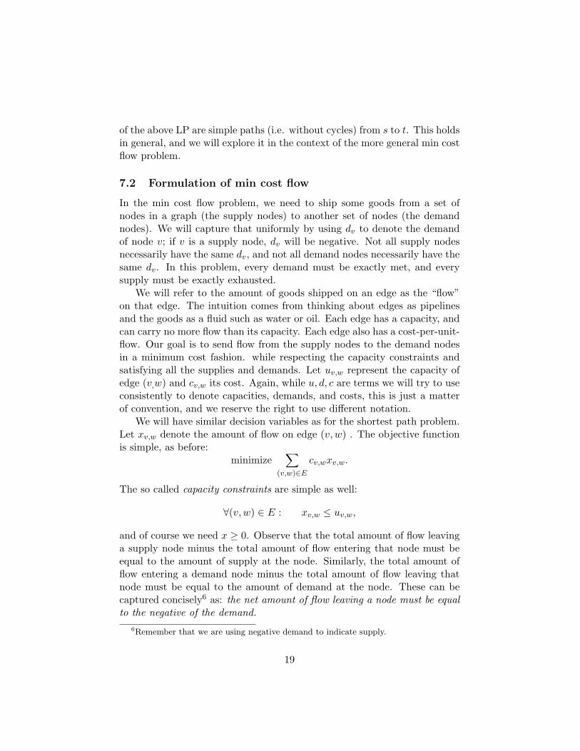
Nodes Edgess (s, p)

Consider the conservation constraint for node p, the other endpoint ofedge (s, p):

xp,s + xp,t − xs,p = 0.

The flow on xs,p is fractional but the RHS of the above equation is integral(in this case, 0), and hence there must be another edge with fractional flowincident on p (i.e. with p as an endpoint). Indeed, there is such an edge, inparticular, edge (p, t). Add p and (p, t) to the table:

Nodes Edgess (s, p)p (p, t)

Consider the conservation constraint for t, the other endpoint of (p, t):

−xr,t − xp,t = −1.

Again, we already know that edge (p, t) has fractional flow. The RHS isagain integral, and hence there must be another edge incident on t whichhas fractional flow. Indeed, such an edge exists, and is (r, t). We will add tand (r, t) to our table:

Nodes Edgess (s, p)p (p, t)t (r, t)

Consider the conservation constraint for r, the other endpoint of (r, t):

xr,t − xq,r = 0.

Again, the RHS is integral, and we have already identified xr,t as fractional.Hence, another edge incident on r must have fractional flow. In this case,(q, r) is such an edge. We add r and (q, r) to the table:

Nodes Edgess (s, p)p (p, t)t (r, t)r (q, r)

23

Consider the other endpoint of (q, r), i.e. q. The conservation constraintfor q is:

xq,r + xq,s − xs,q = 0.

Again, the RHS is integral, and we have already identified (q, r) as an edgethat has fractional flow. Hence, another edge incident on q must have frac-tional flow. In this case, (s, q) is such an edge; we add this edge to our tablealong with node q:

Nodes Edgess (s, p)p (p, t)t (r, t)r (q, r)q (s, q)

There is of course a point to this tedious repetition, and it is time to getto the punch line. The other endpoint of (s, q) is s, which is already in thetable. We have cycled back. Whenever the demands are integral, we will beable to cycle in this fashion, which is the first step in the general proof.

Our cycle is (s, p, t, r, q, s). Notice that some of the edges we identifiedin the table go along this cycle, and some go against. But none of the edgesin the table is at capacity (since the flows on these edges are all fractional)and none of the edges has 0 flow (again, since all the flows are fractional).Hence, for each of these edges, there is some small amount by which theflows can be increased and decreased freely without violating the capacityor non-negativity constraints. This is the second step in the general proof.Observe that the first step crucially used the fact that demands are integral,while the second crucially uses the fact that capacities are integral. In thisexample, the amount by which the flow on any edge in the table can beincreased or decreased freely is 0.5, but this amount may be different forother examples. Choose any amount smaller than this number; in this caselet us choose 0.1.

Let us send additional flow of 0.1 along this cycle (i.e. increase flow by0.1 on the edges in the table that go along this cycle and decrease flow by0.1 on edges that go against.) This gives the solution in figure 4(a). Thismust also satisfy the conservation constraints since the IN and OUT flowsof each node on the cycle are increased by the same amount. Rememberthat we already ensured that the capacity and non-negativity constraintsare satisfied as well, and hence this new solution is also feasible. Now senda flow of 0.1 against the cycle to obtain the feasible solution in figure 4(b).

24

The average of these two new feasible solutions gives us the original fractionsolution from figure 3 and hence the solution in figure 3 can not be basicfeasible. This is the third step in the general proof.

0.6

0

0

st

p

qr

0.4

0.4

0.4

0.6 0.4

0

0

st

p

qr

0.6

0.6

0.6

0.4

(a) (b)

Figure 4: (a) Sending flow along the cycle (s, p, t, r, q, s). (b) Sending flowagainst the cycle (s, p, t, r, q, s).

We can always follow these three steps to prove theorem 7.5 in gen-eral. This theorem also has interesting corollaries about shortest paths andmatchings, since we already showed that these problems can be reduced tominimum cost flow.

Corollary 7.6 Any basic feasible solution to the maximum compatibilitymatching problem must be integral.

Corollary 7.7 Any basic feasible solution to the shortest path problem mustbe integral.

In fact, basic feasible solutions to the shortest path problem have a very nicestructure if the capacities u are set to ∞: any simple path (i.e. no cycles)from s to t is a basic feasible solution, and these are the only basic feasiblesolutions. With capacities set to ∞, if there is a cycle of edges of negativecost, then there is no optimum solution (since sending infinite flow aroundthat cycle results in cost −∞); in all other cases, if there is a path from sto t, commercial solvers such as Excel will return a simple path.

If the goal is to find a negative cost cycle in a graph (eg. for somearbitrage purposes) then set all demands to 0, all capacities to 1, and solvethe minimum cost flow problem. If the optimum solution value is 0, thenthere is no negative cost cycle. If the optimum solution value is -ve, thereis a negative cost cycle and the solution returned by the LP can be used todeduce such a cycle (the cycle will be composed of edges with xv,w = 1).

25

Exercise 7.8 Suppose you are given a variant of the minimum cost flowproblem where there is a lower bound lv,w on the flow on edge (v, w) as wellas an upper bound uv,w, i.e. we have constraints xv,w ≥ lv,w along with thestandard constraints xv,w ≤ uv,w. When can we claim that all basic feasiblesolutions are integral?

Example 7.9 Consider the problem where we are given a graph G = (V,E),success probabilities pv,w on each edge (v, w), a source vertex s and a destina-tion vertex t. Assume edge successes are independent. A path is successful ifall the edges on the path are successful. Accordingly, the success probability,or the reliability, of a path (or a route) R is∏

(v,w)∈R

pv,w.

The goal is to find the most reliable route from s to t. Assume all probabilitiesare between 0 and 1.

Since ln is an increasing function7, maximizing the objective∏(v,w)∈R

pv,w

gives the same route R as maximizing the objective

ln

∏(v,w)∈R

pv,w

.

By using the property that lnxy = ln x + ln y, it is equivalent to maximizethe objective ∑

(v,w)∈R

(ln pv,w) ,

or, to minimize the objective ∑(v,w)∈R

(− ln pv,w) .

This last objective function is just the shortest path objective with costcv,w = − ln pv,w. Thus, we can solve the most reliable path problem by

7The function ln(a), or the natural logarithm of a, is the number b such that a = eb.We have ln 1 = 0; ln 0 = −∞; ln xy = ln x + ln y.

26

solving a shortest path problem using − ln pv,w as the cost of edge (v, w).Since pv,w ≤ 1, we have ln pv,w ≤ 0, or, − ln pv,w ≥ 0. Hence the edge costsin the new shortest path problem are non-negative, and we will not get any-ve cycles. Thus, as long there is a path from s to t, solving the resultingshortest path problem as an LP (with u = either ∞ or 1) will give a simplepath as an optimum solution (assuming we use a typical commercial solver).

7.4 Max-flow

Consider a graph G = (V,E) which has two special vertices s and t. Everyedge has a capacity (but no cost). Instead of having demands on nodes, thegoal is to send as much flow from s to t as possible, while respecting thecapacity constraints. This is known as the max-flow problem, and has manyapplications. In order to model this as an LP, we use the same decisionvariables as for the min-cost-flow problem. The capacity constraints are thesame as before:

∀(v, w) ∈ E : xv,w ≤ uv,w,

and all variables are non-zero:

x ≥ 0.

No node other than s or t can either produce or consume flow, so we havethe following flow conservation constraints for all nodes v other than s andt:

∀v ∈ V − {s, t} : OUTx(v)− INx(v) = 0.

The goal is to maximize the net flow out of s, which must be the same asthe net flow into t since all other nodes can not supply or consume flow.Hence, the objective function is:

maximize INx(t)−OUTx(t),

which completes the LP formulation.There is an interesting way to reduce max-flow to min-cost-flow. Keep

the demands of all nodes as 0. Add a new edge from t to s and set itscapacity to be infinite, and cost −1. For all the original edges in the graphG, keep the original capacity, and set the cost to 0. Since the new edge (t, s)has a cost of -1, and all other edges have a cost of 0, the objective functionof the min-cost-flow problem is equivalent to maximizing the flow on edge(t, s). Since the demands are 0, any flow on the edge (t, s) must then beshipped from s to t through the original network to satisfy the conservationconstraints; this is the original max-flow objective.

27

This allows us to claim that if all the edge capacities are integral, thenall basic feasible solutions to a max-flow-problem are integral.

Exercise 7.10 Suppose there are k special nodes s1, s2, . . . , sk in a graphand j other special nodes t1, t2, . . . , tj. The goal is to maximize the totalflow going from the nodes s1, . . . , sk to t1, . . . , tj. How will you model thisas a standard max-flow problem with only one source node and only oneterminal node?

8 Duality

Duality is a central concept in the theory of optimization. Duals of linearprograms play an important role in understanding, using, and solving linearprograms. Details are in VRM4; in this section, we will merely provideadditional illustrative examples.

8.1 The knapsack problem revisited: duality

Suppose a crime syndicate wants to buy out the thief. They offer to paythe thief a price y1 for the gold, a price y2 for the diamonds, a price y3 forthe silver, and a price y4 per lb for the knapsack8. But the thief can use 2lbs of knapsack capacity and all her gold to generate a profit of 5 units, so2y4 + y1 should be at least 5. Similarly, 3y4 + y2 ≥ 20 and 4y4 + y3 ≥ 3.The syndicate would like to minimize the total price it pays, i.e. minimizey1+y2+y3+4y4. Also, the prices should be non-negative, otherwise the thiefwill hold on to that resource (gold, diamond, silver, or knapsack capacity).This gives us the following LP which the syndicate can use to decide theminimum price:

minimize y1 + y2 + y3 + 4y4

subject to:y1 + 2y4 ≥ 5

y2 + 3y4 ≥ 20y3 + 4y4 ≥ 3

y ≥ 0.

8The Excel spreadsheet names the variables a little differently, with y1 being the pricefor knapsack capacity.

28

Try solving this linear program in Excel. It turns out that y = 〈0, 12.5, 0, 2.5〉is an optimum solution, giving an optimum value of 22.5, or, the same asthe optimum value of the previous LP.

In retrospect, the connection is not really surprising. What is the min-imum total price the thief would settle for? Clearly 22.5, since this is howmuch the thief can make by filling her knapsack and walking away from anydeal being offered by the syndicate. This is an example of duality. Thevariables y1, y2, y3, y4 are called dual variables or dual prices. Duality is avery important concept in economics; in fact prices in the real world canoften best be understood as dual variables.

Recall that N is the number of goods, which gave N variables and N +1constraints in the original LP formulation of the general knapsack problem.Hence, the dual of the knapsack problem has N +1 variables y1, y2, . . . yN+1,and N constraints labeled x1, x2, . . . , xN . The dual is:

minimize

(N∑

i=1

yi

)+ WyN+1

subject to:∀i ∈ {1, . . . , N} : yi + wiyN+1 ≥ vi

y ≥ 0.

8.2 Dual prices as sensitivities

Try increasing the knapsack capacity by 0.1 in the above knapsack example.The optimum solution changes from 22.5 to 22.75. The ratio of change inthe optimum solution to a very small (i.e., infinitesimally small) change inthe right hand side of a constraint (assuming all the variables are to theleft and the constant term is on the right) is known as the sensitivity. Inthis case, the sensitivity to knapsack capacity is (22.75 − 22.5)/0.1 = 2.5.This is not surprising, since any extra knapsack capacity (assuming theextra amount is small) is used for additional gold. Since gold weighs 2lbs,additional capacity used for gold gives us an additional profit of $2.5 perunit of knapsack capacity.

What is surprising is that the dual variable y4 corresponding to theknapsack capacity constraint has value 2.5. In general, a dual variable’svalue in an optimum dual solution is equal to the sensitivity of the primalto the corresponding constraint in the primal. In order to understand this,consider a primal linear program in standard form:

maximize cT · x

29

subject to:Ax ≤ bx ≥ 0

and its dual:

minimize bT · ysubject to:

AT y ≥ cy ≥ 0.

Assume for simplicity that the primal and the dual both have uniqueoptimum solutions. Focus on the optimum solution (say y∗) for the dual.Since the optimum solution is unique, it must be a basic feasible solution.Imagine changing the right hand side of the i-th constraint in the primalslightly: i.e. suppose ci is changed to ci + δi where δi is infinitesimallysmall. For the dual, this only changes the objective function (since the ci’sonly occur in the objective function in the dual) and hence does not impactthe set of basic feasible solutions. For an infinitesimally small change inthe objective, the same basic feasible solution will still remain optimum9.Hence, the change in the optimum objective value for the dual will be δiy

∗i .

By strong duality, this will also be the change in the primal. Hence, thesensitivity of the primal to the i-th constraint is δiy

∗i /δi = y∗i .

If you solve a linear program using Excel, you get a sheet called “sensi-tivity”: these are essentially the dual variables. Thus, we now have anotherconcrete connection between the primal and the dual. This Excel sheet alsohas a “range”. As we change the right hand side of a constraint, we are alsochanging the dual objective function, and when this change is large enough,some other basic feasible solution could become optimum. At this point,the sensitivities of the primal will change; the “range” gives the maximumamount by which we can change the right hand side of a constraint withoutchanging the corresponding dual solution and hence the sensitivities.

If the dual has multiple optimum basic feasible solutions, at least one ofthe ranges will be 0, and you should interpret the sensitivities (or shadowprices as they are sometimes called) with caution. For an illustrative exam-ple, see the sensitivity report you obtain when you set the knapsack capacityto 5 in the above problem and then solve the primal.

9Since y∗ is the unique optimum solution, it must be better than all other basic feasiblesolutions by at least some small positive amount, and an infinitesimally small change inthe objective can not make another basic feasible solution optimum.

30

8.3 The dual of the shortest path problem

Consider a linear program of the form:

minimize cT · xsubject to:

Ax = bx ≥ 0.

Suppose the LP has K constraints and J variables. We will reduce this tothe standard primal form, take the dual, and simplify. We have had somepractice reducing LPs to standard form, so we will go this through quickly.Define

E =

(A−A

), f =

(b−b

), and g = −c.

Now the LP becomes

−maximize gT · xsubject to:

Ex ≤ fx ≥ 0.

We now have 2K constraints and J variables, and the dual is

−minimize fT · zsubject to:

ET z ≥ gz ≥ 0.

The dual has 2K variables, z1, z . . . z2K . We will refer to the first K asp1 . . . pK and the next K as q1 . . . qK . The constraint ET z ≥ g is nowequivalent to AT (p−q) ≥ g and the objective function fT z is now equivalentto bT (p−q). Since p, q always occur together as p−q, we might as well definea new set of variables y1, . . . , yK such that yi = qi − pi. While the variablesz, and hence the variables p, q, were constrained to be non-negative, thevariables y are unconstrained. Replacing fT z by bT (−y), ET z by AT · (−y),g by −c and removing the non-negativity constraints, we have the followingequivalent dual LP:

−minimize cT · (−y)subject to:

AT (−y) ≥ −b,

31

which simplifies to:

maximize cT y

subject to:AT y ≤ b.

What does all this have to do with the shortest path problem? Writethe shortest path problem as:

minimize∑

(v,w)∈E cv,wxv,w

subject to:∀v ∈ V − {s, t} : INx(v)−OUTx(v) = 0

INx(t)−OUTx(t) = 1INx(s)−OUTx(s) = −1

x ≥ 0.

This linear program is now in the form with which we started this sub-section, and hence we can read off its dual using the form that we derived.The primal linear program has M variables, one for each edge (M is thenumber of edges) and N constraints, one for each node. Its dual will haveM constraints (one for each edge) and N variables (one for each node). Wewill label the variables in the dual as yv, where v ∈ V . The dual constraintcorresponding to edge (v, w) is simple: yw−yv ≤ cv,w. The objective functionis yt − ys. The dual is:

maximize yt − ys

subject to:∀(v, w) ∈ E : yw − yv ≤ cv,w.

This is a starkly simple form! Let us interpret this informally. First, observethat in the primal, the constraint IN(s)−OUT (s) = 0 is redundant, since itcan be obtained by adding all the other conservation constraints. Removingthis constraint from the primal is equivalent to setting ys = 0 in the dual,which is what we will implicitly assume from now on. Now, suppose wechange the right hand side of the conservation constraint corresponding tonode v by an infinitesimally small amount δv. This is equivalent to sayingthat the demand of node v has been increased by δv. How will this demandget satisfied? Since there are no capacities in the primal, this demand willget satisfied by sending flow from s to v along a shortest path from s tov; this will incur a cost of δv times the cost of the shortest path from sto v. Hence we expect the dual variables yv to represent the shortest pathdistance between s and v.

32

What about the constraints ∀(v, w) ∈ E : yw − yv ≤ cv,w? This cor-responds to enforcing triangle inequality. If the shortest path length froms to v is yv, then the shortest path length yw from s to w can be at mostyv + cv,w: having arrived at v, we need to pay at most cv,w extra to get tow.

This dual linear program gives rise to the following simple algorithm forfinding shortest paths:

Ford’s algorithm

1. Set ys = 0 and all the other yv’s to ∞ (i.e. some very large number,for example 1 +

∑(v,w)∈E) |cv,w|)

2. while there exists an edge (v, w) such that yw > yv + cv,w set yw =yv + cv,w.

The algorithm is guaranteed to terminate if there are no negative cost cycles.An edge (v, w) such that yw > yv + cv,w is called a violated edge; fixing theedge by setting yw = yv + cv,w is called relaxation. This is the canonicalalgorithm used for most shortest path applications with the main variationbeing in the method to decide which edge is relaxed when there are multipleviolated edges.

Exercise 8.1 Manually simulate Ford’s algorithm for the shortest path ex-ample in figure 1.

Thus, we see how linear program duality can have a great impact in obtain-ing efficient algorithms for important problems.

9 Dynamic Programming – a (very) brief intro-duction

The term dynamic programming is used in multiple ways in optimization.In this class, we will focus on a narrow chunk of dynamic programming,where (a) The overall problem can be decomposed into a tractable numberof subproblems, and (b) Each subproblem can be solved efficiently if allsubproblems of smaller “size” have been solved. Part (a), which involvesonly writing down notation and definitions, is by far the hardest part. Part(b) usually follows, and once we have both parts (a) and (b), solving usingExcel or a programming language is generally trivial. We will illustratethis technique for problems which can be solved using Excel (i.e. where thesubproblems are at most 2-dimensional).

33

9.1 Longest Common Subsequence, aka, Are you a man ora mouse?

The field of computational genomics involves looking at the human (or an-other species’) genome as a sequence of A, C, T, G (the four DNA bases) andusing computation on these sequences to determine genetic functionality,similarity between species, similarity between individuals, disease markers,etc. It is a field which is revolutionizing biology, and dynamic programmingis a key technique.

Rather than survey the entire field, we will discuss a representativeproblem called “Longest Common Subsequence”. Here we are given twosequences of bases P = 〈p1, p2, . . . , pM 〉 and Q = 〈q1, q2, . . . , qN 〉, of lengthsM and N respectively. Remember that a sequence is different from a set inthat the bases are ordered, i.e. they occur in sequence.

A subsequence of a sequence is obtained by deleting an arbitrary num-ber of elements from the sequence; the remaining elements form the sub-sequence. The elements of a subsequence must be in the same order asthe original sequence, but need not be contiguous in the original sequence.Also, the elements in a sequence need not be unique. Given the sequence〈AAACCTTTAAGGGA〉 the following are all subsequences: 〈ACTG〉, 〈AATGGA〉,〈TTT 〉, 〈〉, the last of these being the special sequence called the empty se-quence, of length 0. But 〈TC〉 is not a subsequence. Our goal is to find thelength of the longest common subsequence of P and Q. This is clearly anoptimization problem: notice the term “longest”.

This problem is of key important to phylogeny, the branch of genomics/evolutionthat attempts to make an evolution graph showing how species could haveevolved. Scientists use the longest common subsequence problem (and itsvariants) to determine how similar current or archaeologically obtained genomesof various species are, which allows them to deduce evolutionary distancesbetween species. Variants of this problem are also of great importance indiscovering genetic markers for disease, physical traits, and behavior. Thereare several large supercomputer clusters whose main purpose is to run a toolcalled BLAST which uses variants of the lcs problem to discover similaritybetween genetic material.

Without further ado, we will proceed to step (a). We define L(i, j) to bethe length of the longest common subsequence between the first i elementsof P and the first j elements of Q. The first i elements of P will be denotedP [1 . . . i] the first j elements of Q will be denoted Q[1 . . . j].

Notice that part (a) is very simple to write down, but very perplexingto discover the first time you see a problem. At the same time, it can

34

be very exhilarating to encounter a complex problem, just define the rightsubproblems, and watch the problem solve itself, as this one will. We willdefine L(0, j) = L(i, 0) = 0 for all i, j. The number we are interested in isL(M,N).

Suppose P (i) = Q(j). If the last bases are the same, there is no ad-vantage to not putting them both in the common subsequence, and wehave L(i, j) = 1 + L(i − 1, j − 1). If P (i) 6= Q(j) then every commonsubsequence of P [1 . . . i] and Q[1 . . . j] must involve deleting either the i-thelement of P or the j-th element of Q (or both). Since we do not knowin advance which of the two will be deleted, we can simply set L(i, j) =max{L(i − 1, j), L(i, j − 1)}, and we are done. Notice that to computeL(i, j) we only need values of L with a smaller i or a smaller j so the “size”requirement of part (b) is satisfied. To summarize:

1. Define L(i, 0) = L(0, j) = 0. This correspond to making an (M + 1)×(N + 1) table in Excel and making the first row and the first column0.

2. Fill the rest of the table using the formula

L(i, j) = 1 + L(i− 1, j − 1) if P (i) = Q(j)= max{L(i− 1, j), L(i, j − 1)} other wise.

It is important to note that the above formula will only be used wheni ≥ 1 and j ≥ 1 and hence all the L values used have been previouslydefined.

If your Excel tables are properly set up, the values P (i), Q(j), L(i−1, j), L(i, j−1), L(i, j) are all easy to locate using Excel style addressing (using $’s to fixthe rows/columns where you look up P , Q). Just type in the above formulain the cell corresponding to L(1, 1) and copy/paste the formula into the restof the table. Since the formula only refers to cells of a smaller “size” i.e.smaller i or j, there will be no cyclic definitions and Excel will fill the wholetable. You can then read off the value of L(M,N). The Excel file lcs.xlsprovides an example. It is clear that you can solve this problem easily inany high level programming language. We will now see another interestingapplication of lcs:

Example 9.1 You are given a sequence P of numbers. Find the largestnon-decreasing subsequence of P .

The above problem can be solved by sorting P ; let Q be the sorted sequence.The lcs of P and Q solves the problem.

35