MSE WALL AND REINFORCEMENT TESTING AT …...reinforced soil mass as a rigid block, (ii) the assumption of strain compatibility between the reinforcement and the soil, (iii) the assumption

MSE WALL AND REINFORCEMENT TESTING

AT MUS-16-7.16 BRIDGE SITE

State Job Number: 14735

Final Report

BY

ROBERT Y. LIANG DEPARTMENT OF CIVIL ENGINEERING

UNIVERSITY OF AKRON AKRON, OHIO 44325-3905

Prepared in Cooperation with Ohio Department of Transportation and the

U.S Department of Transportation, Federal Highway Administration

September 2004

2

The primary objectives of this research are to (i) plan and carry out an instrumentation monitoring and field pullout testing program on an instrumented 52 ft (15.85 m) high reinforced earth wall, (ii) examine the adequacy of the current practice of design and analysis of reinforced earth walls with emphasize on the method recommended by the FHWA Design Manual and the Coherent Gravity Method, and (iii) develop a new method for design and analysis of reinforced earth wall. The field instrumentation program has provided measurements of reinforcement working forces, lateral earth pressures, vertical earth pressures, and the deflections at wall facing. The comparisons made between the field measurements and the current method adopted by the FHWA indicated that significant errors have occurred, especially in the case of slopping backfill. The results also indicated that the reinforcements and the wall facing have significantly influenced the vertical earth pressure. The vertical earth pressure could be reasonably approximated by the uniform pressure distribution leading to possible savings in the cost of reinforced earth walls. A new method has also been developed and presented in this report. The method is called the Virtual Soil Wedge (VSW) method, and it has been derived by studying the analogous retaining actions of the reinforcements and the retaining soil slopes. The method has been shown to accurately predict the reinforcement working forces, lateral earth pressures, and the reinforcement pullout resistance. The VSW method requires the evaluation of a new factor called the scaling factor, f, using field measurements of different reinforcement and soil combinations.

MSEW, Reinforced earth wall, field instrumentation-monitoring, field pullout tests, a new design/analysis method- Virtual Soil Wedge method.

MSE WALL AND REINFORCEMENT TESTING

AT MUS-16-7.16 BRIDGE SITE

State Job Number: 14735

Final Report

BY

ROBERT Y. LIANG DEPARTMENT OF CIVIL ENGINEERING

UNIVERSITY OF AKRON AKRON, OHIO 44325-3905

Prepared in Cooperation with Ohio Department of Transportation and the

U.S Department of Transportation, Federal Highway Administration

September 2004

DISCLAIMER STATEMENT

The contents of this report reflect the views of the authors who are responsible for the

fact and accuracy of the data presented herein. The contents do not necessarily reflect the

official views or policies of the Ohio Department of Transportation or Federal Highway

Administration. This report does not constitute a standard, specification or regulation.

ABSTRACT

The assumptions involved in the current method recommended in the FHWA Design

Manual and the Coherent Gravity method for design of reinforced earth walls resulted in

many discrepancies. These most influential assumptions are (i) the treatment of the

reinforced soil mass as a rigid block, (ii) the assumption of strain compatibility between

the reinforcement and the soil, (iii) the assumption of no frictional stresses along the soil

horizontal slices, and (iv) the ignorance of the effects of the reinforcement lengths and

stiffness on the vertical and horizontal stresses and the working forces of the

reinforcements. These assumptions resulted, in many cases, in either overestimating or

underestimating the working forces in the reinforcement, as well as the vertical and

lateral earth pressures within the reinforced soil mass. They were also responsible for the

errors in obtaining the reinforcement resistance to pullout, and the active and effective

lengths of reinforcements.

The main objective of this research is to carry out an instrumentation monitoring

and field-testing program on a newly constructed 52 ft (15.85 m) high MSE abutment

wall on the Old Schoolhouse Road in Muskingum County, Ohio. The instrumentation

plan included strain gages spot-welded to pre-selected reinforcement strips, earth

pressure cells located at the bottom of the reinforced soil mass, and contact pressure cells

embedded in the concrete facing. Four field pullout tests have also been conducted

corresponding to four different overburden depths. The research resulted in the

development of a new method that can be used to accurately analyze and effectively

design the reinforced earth walls. This method, called the Virtual Soil Wedge (VSW)

method, has been theoretically developed to account for the influences of the

reinforcement spacing, length, and location relative to the height of the wall in the

calculation of the working forces of the reinforcement, the lateral earth pressures, and the

pullout factors of the reinforcements. This method has introduced two new factors: an

embracement factor that relates the reinforcement layouts to the lateral earth pressures,

and a scaling factor that accounts for the roughness, type and shape of the reinforcement,

and the type and size of the backfill soil. The scaling factors for different soil and

reinforcement combinations should be evaluated using field measurements or

experimental data.

The field measurements made at the Schoolhouse Road wall were compared with

the method recommended by the FHWA Design Manual and the VSW method developed

in this research. The FHWA recommended method was shown to be only convenient for

the case of walls with simple geometry. However, for walls with slopping backfill

surcharge, significant errors were observed. The VSW method, on the other hand, was

shown to be capable of accurately predicting the measured maximum reinforcement

forces and their locations, the lateral earth pressures, and the pullout resistance of the

reinforcement. The presence of reinforcements has influenced the vertical earth pressure

values throughout the construction period. This, in turn, has influenced the distribution of

the pullout factors, F*, with the overburden depth. Combining the VSW method with the

basic equation defining the pullout resistance of the reinforcement, resulted in the

development of a relationship defining the pullout factors of the reinforcement as a

function of the reinforcement spacing, length and locations within the reinforced earth

walls.

i

TABLE OF CONTENTS

Page

LIST OF TABLES v

LIST OF FIGURES vii

ABSTRACT xxv

CHAPTER 1 INTRODUCTION AND RESEARCH MERIT

1.1 INTRODUCTION 1

1.2 STATEMENT OF THE PROBLEM AND SIGNIFICANCE OF WORK 6

1.3 RESEARCH OBJECTIVES 12

CHAPTER 2 LITERATURE SURVEY 15

2.1 INTERNAL STABILITY 15

2.1.1 Lateral earth pressure and internal failure surface 16

2.1.2 Reinforcement’s pullout resistance 34

2.2 EXTERNAL STABILITY 38

2.3 COMPACTION INDUCED STRESSES 42

2.4 FINIT ELEMENT ANALYSIS 46

2.5 CASE STUDIES 50

2.5.1 Christopher (1993) 50

2.5.2 Minnow Creek wall 53

ii

CHAPTER 3 INSTRUMENTATION AND FIELD MONITORING PROGRAM

3.1 PROJECT DESCRIPTION 74

3.2 GEOLOGY OF THE SITE 75

3.3 MATERIAL PROPERTIES 76

3.3.1 Backfill and Foundation Materials 76

3.3.2 Reinforcement and facing 77

3.4 FIELD INSTRUMENTATION AND TESTING PLAN 77

3.4.1 Instrumentation plan 77

3.4.2 Field pullout test program 84

CHAPTER 4 FIELD MONITORING RESULTS

4.1 AXIAL FORCES IN REINFORCEMENT 106

4.2 PRESSURE MEASUREMENTS 115

4.2.1 Vertical pressure measurements 115

4.2.2 Horizontal pressures measurements 117

4.3 FIELD PULLOUT RESISTANCE 118

4.4 FIELD SETTLEMENT AND DEFORMATION MEASUREMENTS 120

4.4.1 Vertical settlement 120

4.4.2 Lateral wall deformation 122

4.5 COMPARISON WITH CURRENT PRACTICE 124

iii

CHAPTER 5 NEW CONCEPT IN DESIGN AND ANALYSIS OF REINFORCED EARTH WALLS- PART I: THEORY AND DEVELOPMENT.

5.1 INTRODUCTION 254

5.2 VIRTUAL SOIL WEDGE SUPPORT CONCEPT 254

5.3 VIRTUAL SOIL WEDGE ANALYSIS 256

5.3.1 Virtual Soil Wedge Analysis 256

5.3.2 Reinforcement maximum axial forces 264

5.4 SIMPLIEFIED APPROACH 269

5.5 ANALYSIS AND DESIGN PROCEDURES 276

5.5.1 Analysis procedure 276

5.5.2 Design procedure 277

CHAPTER 6 VALIDATION OF THE VIRTUAL SOIL WEDGE METHOD


6.2 CASE STUDIES 290

6.2.1 Schoolhouse MSE-wall 290

6.2.2 Christopher (1993) 299

6.2.3 Minnow Creek Wall (Rusner, 1999) 300

CHAPTER 7 REINFORCEMENT-SOIL INTERACTION USING VIRTUAL SOIL WEDGE METHOD


7.2 DEVELOPMENT OF A RATIONAL FORMULA 319

iv

7.2.1 Vertical earth pressure 321

7.2.2 Pullout Resistance of Reinforcement 326

7.3 CASE STUDY: SCHOOLHOUSE RD MSE WALL 328

7.3.1 Summary of field measurements 328

7.3.2 Pullout analysis using the VSW-method 329

CHAPTER 8 SUMMARY AND CONCLUSIONS

8.1 SUMMARY OF RESEARCH FINDINGS 338

8.2 CONCLUSIONS 347

8.3 IMPLEMENTATION RECOMMENDATIONS 351

8.4 RECOMMENDATIONS FOR FUTURE RESEARCH 352

REFERENCES 354

APPENDIX A1 MEASUREMENT AT THE 52 FT (15.85 m) HIGH SECTION AT THE MEDIAN (SECTION A)

A1-1

APPENDIX A2 MEASUREMENT AT THE 52 FT (15.85 m) HIGH SECTION AT THE MEDIAN (SECTION B)

A2-1

APPENDIX A3 MEASUREMENT AT THE 30 FT (9.1 m) HIGH SECTION AT THE WING WALL (SECTION C)

A3-1

APPENDIX A4 MEASUREMENT AT THE 20 FT (6 m) HIGH SECTION AT THE WING WALL (SECTION D)

A4-1

APPENDIX A5 LONG-TERM STRAIN GAGE MONITORING RESULTS A5-1

APPENDIX B DERIVATION OF VSW METHOD B-1

v

LIST OF TABLES

Table TITLE Page

2.1 Pullout test program by Christopher (1993).

52

2.2 Summary of field test program by Christopher (1993).

53

3.1 Locations and numberings of the instrumented reinforcement straps for sections A and B.

81

3.2 Locations of strain gages along instrumented straps in sections A and B.

81

3.3 Locations and numberings of the instrumented reinforcement straps for section C.

82

3.4 Locations of strain gages along instrumented straps in section C.

82

3.5 Locations and numberings of the instrumented reinforcement straps for section D.

83

3.6 Locations of strain gages along instrumented straps in section D.

83

4.1 Maximum reinforcement forces based on measured reinforcement strains in the 52-ft (15.85 m) tall section.

110

4.2 Maximum reinforcement forces based on measured reinforcement strains in the 30-ft (9.1 m) tall section.

110

4.3 Maximum reinforcement forces based on measured reinforcement strains in the 20-ft (6 m) tall section.

111

4.4 Maximum reinforcement forces based on measured reinforcement strains in the 52-ft (15.85 m) tall section due to surface surcharge.

114

4.5 Maximum reinforcement forces based on measured reinforcement strains in the 30-ft (9.1 m) tall section due to surface surcharge.

114

4.6 Maximum reinforcement forces based on measured reinforcement strains in the 20-ft (6 m) tall section due to surface surcharge.

115

vi

Table

TITLE

Page

4.7 Summary of load-displacement curves for pullout test straps. 120

4.8 Settlement in inches of foundation material 10 ft (3 m) behind the eastern wall.

122

6.1 Maximum axial forces per unit width measured in instrumented straps in the 52 ft (15.85 m) high section.

291

6.2 Calculations of lateral earth pressures using the VSW-method for Schoolhouse wall with the FHWA distribution for the effective length of reinforcement (52 ft (15.85 m) section).

295

6.3 Calculated active and effective lengths of reinforcement and the actual embracement factors (52 ft (15.85) section).

296

6.4 Maximum reinforcement forces based on measured reinforcement strains in the 30 ft (9.1 m) high section.

298

6.5 Calculations using VSW method for the 30 ft (9.1 m) section 298

6.6 Calculation of lateral earth pressure for wall-1 (Christopher, 1993) using the VSW-method.

300

6.7 Calculations of lateral earth pressures using the VSW-method for Minnow-Creek wall

302

7.1 Calculations of lateral earth pressures using the VSW-method. 331

vii

LIST OF FIGURES

Figure page

1.1 Typical reinforced earth wall. 13

1.2 External stability modes for reinforced earth walls.

14

2.1 a) Distribution of the theoretical coefficient of lateral earth pressure with depth,

b) Theoretical and experimental failure surfaces, and

c) Computed and measured heights of model walls a failure. (Juran, 1977)

55

2.2 Active failure wedges for reinforced soil walls. 56

2.3 Earth pressure distribution within inextensible reinforced soil per the Coherent Gravity method (Bassett and Last, 1978).

56

2.4 Theoretical distributions for the coefficient of lateral earth pressure with depth. (reproduced from Bonaparte and Schmertmann, 1987)

57

2.5 Compatibility curve between soil and reinforcement (Jewell, 1985).

58

2.6 Internal equilibrium in reinforced earth walls.

59

2.7 Lateral earth pressure distribution for ribbed steel reinforcement per the FHWA Design Manual (Elias and Christopher, 1996).

60

2.8 Measured maximum forces in the geosynthetic reinforcements versus the values predicted using the ko-stiffness method produced by Allen and Bathurst (2001).

61

2.9 Measured maximum forces in reinforcements with different types versus the predicted values using the ko-stiffness method.

62

2.10

Soil-reinforcement interaction: a) frictional resistance, b) friction-bearing for ribbed reinforcement, and c) friction-bearing for steel mesh reinforcement.

63

viii

Figure Page

2.11 External forces acting on reinforced earth walls. 64

2.12 Distributions of pressure under reinforced earth walls: b) Trapezoidal, c) Meyerhof’s.

65

2.13 Plastic zones near roller-soil contact area (Duncan and Seed, 1986).

66

2.14 Assumed stress path due to compaction (Duncan and Seed, 1986).

67

2.15 Schematic of the skin-plate reinforced wall modeled by Chang and Forsyth (1977).

68

2.16 Mohr-Coulomb yield surface confined by the lower and upper bounds (Yu and Sloan, 1997).

69 2.17 Measured maximum strains in the reinforcements in wall

1 (Christopher, 1993).

70

2.18 Geometry of Minnow Creek MSE-wall. 71

2.19 Cross-section of the Minnow Creek wall. 72

2.20 Measured maximum tensile forces in the reinforcements in Creek Minnow wall (Runser, 1999).

73

3.1 Schematics of the instrumented MSE wall: a) Front projection, and b) Plan view.

85

3.2 Construction activities for the Schoolhouse MSE-wall. 86

3.3a Soil boring data for SC-2. 87

3.3b Soil boring data for SC-2a. 88

3.4 Soil profile along the eastern (instrumented) wall. 89

3.5 Instrumented 52-ft (15.85 m) high wall sections (Sections A and B).

90

ix

Figure Page

3.6 Instrumented 30-ft (9.1 m) high wall section (Section C). 91

3.7 Instrumented 20-ft (6 m) high wall section (Section D). 92

3.8 Mounting of strain gages to the straps (spot welding). 93

3.9 Temporary storage of instrumented straps. 94

3.10 Installation of instrumented straps. 95

3.11 Covering of instrumented straps by soil backfill. 95

3.12 Installation of vertical pressure transducer cells. 96

3.13 Contact pressure cell and installation and temporary protection. 97

3.14 Steel cabinet containments and protection of data acquisition. 98

3.15 Piles, and piles sleeves. 99

3.16 End of construction of the project. 100

3.17 Pullout test details: (a) soil overburden conditions, (b) front view and cross-section of test setup.

101

3.18 Configuration of gages for pullout test strap. 102

3.19 Field pullout test strap-panel configuration. 103

3.20 Schematics of pullout test setup: Loading jack and reaction frame.

104

3.21 Field pullout test setup and loading frame. 105

4.1a Axial force measurements in the strap located at 1.25 ft (0.4 m) above the L.P in the 52 ft (15.85 m) tall section (50.75 ft (15.5 m)) below wall coping).

127

x

Figure Page

4.1b Measured force profiles in the strap located at 1.25 ft (0.4 m) above the L.P in the 52 ft (15.85 m) tall section ( 50.75 ft (15.5 m)) below wall coping).

128

4.2a Axial force measurements in the strap located at 6.25 ft (1.9 m) above the L.P in the 52 ft (15.85 m) tall section (46.25 ft (14.1 m)) below wall coping).

129

4.2b Measured force profiles in the strap located at 6.25 ft (1.9 m) above the L.P in the 52 ft (15.85 m) tall section (46.25 (14.1 m) ft below wall coping).

130

4.3a Axial force measurements in the strap located at 11.25 ft (3.4 m) above the L.P in the 52 ft ( 15.85 m) tall section ( 41.25 ft (12.6 m) below wall coping).

131

4.3b Measured force profiles in the strap located at 11.25 ft (3.4 m) above the L.P in the 52 ft (15.85 m) tall section (41.25 ft (12.6 m)) below wall coping).

132

4.4a Axial force measurements in the strap located at 16.25 ft (5 m) above the L.P in the 52 ft (15.85 m) tall section (36.25 ft (11 m) below wall coping).

133

4.4b Measured force profiles in the strap located at 16.25 ft (5 m) above the L.P in the 52 ft (15.85 m) tall section (36.25 ft (11 m) below wall coping).

134

4.5a Axial force measurements in the strap located at 23.75 ft (7.2 m) above the L.P in the 52 ft (15.85 m) tall section (28.75 ft (8.8 m) below wall coping).

135

4.5b Measured force profiles in the strap located at 23.75 ft (7.2 m) above the L.P in the 52 ft (15.85 m) tall section (28.75 ft (8.8 m) below wall coping).

136

4.6a

Axial force measurements in the strap located at 28.75 ft (8.8 m) above the L.P in the 52 ft (15.85 m) tall section (23.75 ft (7.2 m) below wall coping).

137

xi

Figure

Page

4.6b Measured force profiles in the strap located at 28.75 ft (8.8 m)

above the L.P in the 52 ft (15.85 m) tall section (23.75 ft (7.2 m) below wall coping).

138


139


140


141


142


143


144

4.10a Axial force measurements in the strap located at 3.25 ft (1 m) above the L.P in the 30 ft (9.1 m) tall section (26.75 ft (8.2 m) below wall coping).

145

4.10b Measured force profiles in the strap located at 3.25 ft (1 m) above the L.P in the 30 ft (9.1 m) tall section (26.75 ft (8.2 m) below wall coping).

146


147

xii

Figure Page


148


149


150

4.13a Axial force measurements in the strap located at 13.25 ft (4 m) above the L.P in the 30 ft (9.1 m) tall section (16.75 ft (5.1 m) below wall coping).

151

4.13b Measured force profiles in the strap located at 13.25 ft (4 m) above the L.P in the 30 ft (9.1 m) tall section (16.75 ft (5.1 m) below wall coping).

152

4.14a Axial force measurements in the strap located at 18.25 ft (5.6 m) above the L.P in the 30 ft (9.1 m) tall section (11.75 ft below wall coping).

153


154

4.15a Axial force measurements in the strap located at 23.25 ft (7.1 m) above the L.P in the 30 ft (9.1 m) tall section (6.75 ft (2 m) below wall coping).

155

4.15b Measured force profiles in the strap located at 23.25 ft (7.1 m) above the L.P in the 30 ft (9.1 m) tall section (6.75 ft (2 m) below wall coping).

156

4.16a Axial force measurements in the strap located at 1.25 ft (0.4 m) above the L.P in the 20 ft (6 m) tall section (18.75 ft (5.7 m) below wall coping).

157

xiii

Figure

Page

4.16b Measured force profiles in the strap located at 1.25 ft (0.4 m) above the L.P in the 20 ft (6 m) tall section (18.75 ft (5.7 m) below wall coping).

158

4.17a Axial force measurements in the strap located at 3.75 ft (1.1 m) above the L.P in the 20 ft (6 m) tall section (16.25 ft (5 m) below wall coping).

159

4.17b Measured force profiles in the strap located at 3.75 ft (1.1 m) above the L.P in the 20 ft (6 m) tall section ( 16.25 ft (5 m) below wall coping).

160

4.18a Axial force measurements in the strap located at 6.25 ft (1.9 m) above the L.P in the 20 ft (6 m) tall section (13.75 ft below wall coping).

161


162

4.19a Axial force measurements in the strap located at 11.25 ft (3.4 m) above the L.P in the 20 ft (6 m) tall section (8.75 ft (2.7 m) below wall coping).

163


164

4.20a Axial force measurements in the strap located at 16.25 ft (5 m) above the L.P in the 20 ft (6 m) tall section (3.75 ft (1.1 m) below wall coping).

165

4.20b Measured force profiles in the strap located at 16.25 ft (5 m) above the L.P in the 20 ft (6 m) tall section (3.75 ft (1.1 m) below wall coping).

166

4.21 Axial force measurements in the strap located at 1.25 ft (0.4 m) above the L.P in the 52 (15.85 m) tall section (50.75 ft (15.5 m)) below wall coping) after reinforcement-backfilling after reinforcement-backfilling.

167

xiv

Figure

Page

4.22 Figure 4.22 Axial force measurements in the strap located at 6.25 ft (1.9 m) above the L.P in the 52 ft (15.85 m) tall section (46.25 ft (14.1 m) below wall coping) after reinforcement-backfilling after reinforcement-backfilling.

168

4.23 Axial force measurements in the strap located at 11.25 ft (3.4 m) above the L.P in the 52 ft (15.85 m) tall section ( 41.25 ft (12.6 m)below wall coping) after reinforcement-backfilling.

169

4.24 Axial force measurements in the strap located at 16.25 ft (5 m) above the L.P in the 52 ft (15.85 m) tall section ( 36.25 ft (11 m) below wall coping) after reinforcement-backfilling.

170

4.25 Axial force measurements in the strap located at 23.75 ft (7.2 m) above the L.P in the 52 ft (15.85 m) tall section (28.75 ft (8.8 m) below wall coping) after reinforcement-backfilling.

171


172


173


174


175

4.30 Axial force measurements in the strap located at 3.25 ft (1 m) above the L.P in the 30 ft (9.1 m) tall section (26.75 ft (8.2 m) below wall coping) after reinforcement-backfilling.

176


177

xv

Figure

Page

4.32 Axial force measurements in the strap located at 8.25 ft (2.5 m) above the L.P in the 20 ft (6 m) tall section (21.75 ft (6.6 m) below wall coping) after reinforcement-backfilling.

178

4.33

Axial force measurements in the strap located at 13.25 ft (4 m) above the L.P in the 30 ft (9.1 m) tall section (16.75 ft (5.1 m) below wall coping) after reinforcement-backfilling.

179


180

4.35 Axial force measurements in the strap located at 23.25 ft above the L.P in the 30 ft (9.1 m) tall section (6.75 ft (2 m) below wall coping) after reinforcement-backfilling.

181

4.36 Axial force measurements in the strap located at 28.25 ft above the L.P in the 30 ft (9.1 m) tall section (1.75 ft (0.5 m) below wall coping) after reinforcement-backfilling.

182


183

4.38 Axial force measurements in the strap located at 3.75 ft (1.1 m) above the L.P in the 20 ft (6 m) tall section ( 16.25 ft (5 m) below wall coping) after reinforcement-backfilling.

184


185


186

4.41 Axial force measurements in the strap located at 16.25 ft (5 m) above the L.P in the 20 ft (6 m) tall section (3.75 ft (1.1 m) below wall coping) after reinforcement-backfilling.

187

xvi

Figure

Page


188

4.43 Measured force profiles in the strap located at 1.25 ft (0.4 m) above the L.P in the 52 ft (15.85 m) high section ( 50.75 ft (15.5 m)) below wall coping) throughout construction period.

189

4.44 Measured force profiles in the strap located at 6.25 ft (1.9 m) above the L.P in the 52 ft (15.85 m) high section (46.25 ft (14.1 m) below wall coping) throughout construction period.

190

4.45 Measured force profiles in the strap located at 11.25 ft (3.4 m) above the L.P in the 52 ft (15.85 m) high section ( 41.25 ft (12.6 m)below wall coping) throughout construction period.

191

4.46 Measured force profiles in the strap located at 16.25 ft (5 m) above the L.P in the 52 ft (15.85 m) high section ( 36.25 ft (11 m) below wall coping) throughout construction period.

192


193


194


195

4.50 Measured force profiles in the strap located at 41.25 ft (12.6 m)above the L.P in the 52 ft (15.85 m) high section (11.25 ft (3.4 m) below wall coping) throughout construction period.

196


197

xvii

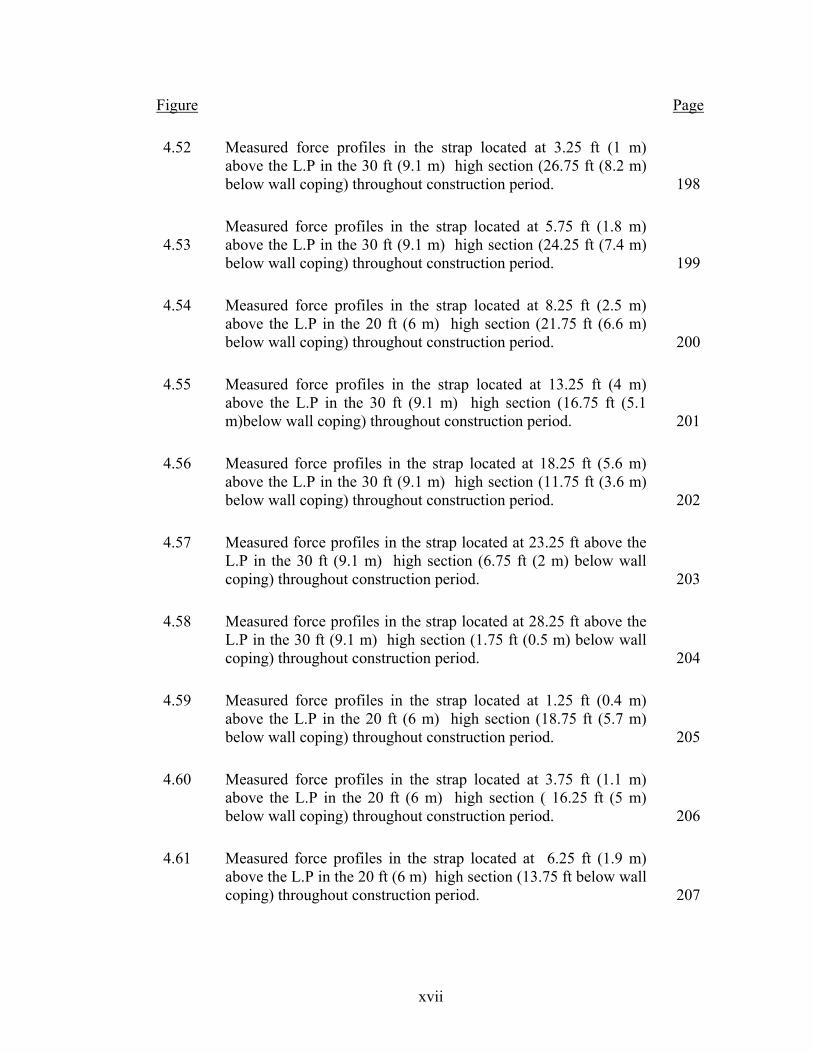
Figure

Page

4.52 Measured force profiles in the strap located at 3.25 ft (1 m) above the L.P in the 30 ft (9.1 m) high section (26.75 ft (8.2 m) below wall coping) throughout construction period.

198

4.53

Measured force profiles in the strap located at 5.75 ft (1.8 m) above the L.P in the 30 ft (9.1 m) high section (24.25 ft (7.4 m) below wall coping) throughout construction period.

199

4.54 Measured force profiles in the strap located at 8.25 ft (2.5 m) above the L.P in the 20 ft (6 m) high section (21.75 ft (6.6 m) below wall coping) throughout construction period.

200

4.55 Measured force profiles in the strap located at 13.25 ft (4 m) above the L.P in the 30 ft (9.1 m) high section (16.75 ft (5.1 m)below wall coping) throughout construction period.

201


202

4.57 Measured force profiles in the strap located at 23.25 ft above the L.P in the 30 ft (9.1 m) high section (6.75 ft (2 m) below wall coping) throughout construction period.

203

4.58 Measured force profiles in the strap located at 28.25 ft above the L.P in the 30 ft (9.1 m) high section (1.75 ft (0.5 m) below wall coping) throughout construction period.

204


205

4.60 Measured force profiles in the strap located at 3.75 ft (1.1 m) above the L.P in the 20 ft (6 m) high section ( 16.25 ft (5 m) below wall coping) throughout construction period.

206

4.61 Measured force profiles in the strap located at 6.25 ft (1.9 m) above the L.P in the 20 ft (6 m) high section (13.75 ft below wall coping) throughout construction period.

207

xviii

Figure Page

4.62 Measured force profiles in the strap located at 11.25 ft (3.4 m) above the L.P in the 20 ft (6 m) high section (8.75 ft below wall coping) throughout construction period.

208

4.63

Measured force profiles in the strap located at 16.25 ft (5 m) above the L.P in the 20 ft (6 m) high section (3.75 ft (1.1 m) below wall coping) throughout construction period.

209


210

4.65a Built-up vertical earth pressures beneath the reinforced soil mass throughout construction period (52 ft (15.85 m) tall section A).

211

4.65b Built-up vertical earth pressures beneath the reinforced soil mass throughout construction period (52 ft (15.85 m) tall section B).

212

4.66a Vertical earth pressure measurements versus the height of reinforced backfill in the 52 ft (15.85 m) tall section (section A).

213

4.66b Vertical earth pressure measurements versus the height of reinforced backfill in the 52 ft (15.85 m) (15.85 m) (15.85 m) tall section (section B).

214

4.67 Vertical earth pressure profiles along the base of the reinforced soil at different construction stages.

215

4.68a Lateral earth pressure measured 10 ft (3 m) above the leveling pad on the wall facing during construction (Section A).

216

4.68b Lateral earth pressure measurements with fill height above pressure sensor located 10 ft (3 m) above the leveling pad on the wall facing during construction (section A).

217

4.69a Lateral earth pressure measured 5 ft (1.5 m) above the leveling pad on the wall facing during construction (Section B).

218

xix

Figure Page

4.69b Lateral earth pressure measurements with fill height above pressure sensor located 5 ft (1.5 m) above the leveling pad on the wall facing during construction (Section B).

219

4.70a Lateral earth pressure measured 10 ft (3 m) above the leveling pad on the wall facing during construction.

220

4.70b Lateral earth pressure measurements with fill height above pressure sensor located 10 ft (3 m) above the leveling pad on the wall facing during construction.

221

4.71 Pullout load-displacement curves for the four pullout test straps. 222

4.72 Axial force profiles measured along the pullout strap tested under embedded 14.5 ft (4.4 m) below grade under different test loads.

223


224


225

4.75 Axial force profiles measured along the pullout strap tested under embedded 42.5 ft (13 m) below grade under different test loads.

226

4.76 Deduced frictional stresses along the pullout strap tested under embedded 14.5 ft (4.4 m) below grade under different test loads.

227


228


229

4.79 Deduced frictional stresses along the pullout strap tested under embedded 42.5 ft (13 m) below grade under different test loads.

230

4.80 Deduced friction factors for the pullout strap tested under embedded 14.5 ft (4.4 m) below grade under different test loads.

231

xx

Figure Page


232


233

4.83 Deduced friction factors for the pullout strap tested under embedded 42.5 ft (13 m)below grade under different test loads.

234

4.84 Coefficient of friction (pullout factors) for the four pullout test straps.

235

4.85 Locations of the Settlement plates. 236

4.86 Settlement measurements on the eastern wall at different construction corresponding dates.

237

4.87 Wall settlements since October 14th 2000. 238

4.88 Wall deflections in the East-West direction as measured by the wall front survey point at the 52 ft (15.85 m) (15.85 m) (15.85 m) high wall section.

239

4.89 Wall deflections in the North-South direction as measured by the wall front survey point at the 52 ft (15.85 m) (15.85 m) (15.85 m) high wall section.

240

4.90 Wall deflections in the East-West direction as measured by the wall front survey point at the 30 ft (9.1 m) high wall section.

241

4.91 Wall deflections in the North-South direction as measured by the wall front survey point at the 30 ft (9.1 m) high wall section.

242

4.92 Lateral deflections along the height of the 52 ft (15.85 m) (15.85 m) section.

243

4.93 Lateral deflections along the height of the 30 ft (9.1 m) section. 244

xxi

Figure Page

4.94 Deflected shapes of reinforced earth wall: a) influence of wall settlement, and b) influence of wall geometry.

245

4.95 Comparison of the reinforcement maximum axial forces with the FHWA’s method for the 52 ft (15.85 m) (15.85 m) tall section.

246

4.96 Comparison of the locations of reinforcement maximum axial forces with the FHWA’s method.

247

4.97 Comparison of the reinforcement maximum axial forces with the FHWA’s method for the 30 ft (9.1 m) tall section.

248

4.98 Comparison of the reinforcement maximum axial forces with the FHWA’s method for the 20 ft (6 m) tall section.

249

4.99 Comparison of the locations of reinforcement maximum axial forces with the FHWA’s method for the 30 ft (9.1 m) tall section.

250

4.100 Comparison of the locations of reinforcement maximum axial forces with the FHWA’s method for the 20 ft (6 m) tall section.

251

4.101 Comparison of the measured lateral earth pressure coefficients with the FHWA’s design method.

252

4.102 Comparison of the measured vertical pressure beneath the reinforced soil with the trapezoidal and Meyerhof’s distributions.

253

5.1 a) Descriptive schematic of the two stabilizing systems, b) Equivalent reinforcement to compensate the virtual stable soil slope.

279

5.2 a) transformation of reinforcement elements into an equivalent soil-retaining slope, and b) the equivalent virtual soil slope.

280

5.3 System of forces in the virtual soil-retaining mass. 281

5.4 System of forces and resistances on a) segment I, and b) segment II.

282

xxii

Figure Page

5.5 System of forces and resistances on segment III. 283

5.6 a) Force profile along a reinforcement layer, b) working friction stress along a reinforcement layer, c) working friction resistance stresses for all reinforcement layers.

284

5.7 Frictional working resistance a) along reinforcement working length, and b) along the base of soil-retaining layer

285

5.8 Frictional resistances along the second reinforcement layer. 286

5.9 Effect of underlying reinforcements on the current reinforcement layer.

287

5.10 Sample distributions for the lateral earth pressure coefficients with the reinforced earth walls.

288

5.11 Deduced distributions for the active lengths of the reinforcements, each corresponding to the lateral earth pressure distributions in 5.10.

289

6.1 Axial force profiles measured at the 52 ft (15.85 m) (15.85 m) (15.85 m) high sections at the end of construction with no surface load (forces in lb/ft).

303

6.2 Locations of maximum tensile forces in the reinforcement observed at the Schoolhouse MSE wall.

304

6.3 Measured vs. predicted k/ka values for the Schoolhouse MSE wall.

305

6.4 Observed limiting equilibrium surface versus the VSW method predictions, and the FHWA assumption.

306

6.5 Comparison of the measured lateral earth pressure coefficients with the predictions of the VSW using the VSW distribution for the line of limiting equilibrium.

307

xxiii

Figure

Page

6.6 Measured axial reinforcement loads compared to the FHWA’s approach and the predictions of the VSW-method for the Schoolhouse wall.

338

6.7 VSW-method predictions for k/ka under current and expected ultimate loading conditions compared with the current measurements and FHWA’s design.

309

6.8 VSW-method predictions for axial forces under current and expected ultimate loading conditions compared with the current measurements and FHWA’s design.

310

6.9 Axial force profiles measured at the 30 ft (9.1 m) high sections at the end of construction (forces in lb/ft).

311

6.10 Transformation of surface inclination into equivalent reinforced soil mass.

312

6.11 Measured vs. predicted reinforcement forces using the VSW method for the 30 ft (9.1 m) high section at the Schoolhouse Road MSE wall.

313

6.12 Comparison between the calculated and measured lateral earth pressure coefficients for Christopher (1993) 20 ft (6 m) test high wall.

314

6.13 Comparison between the calculated and the measured reinforcement forces for Christopher (1993) 20 ft (6 m) test high wall.

315

6.14 Comparison between the calculated and measured lateral earth pressure coefficients for Minnow-Creek wall.

316

6.15 Comparison between the calculated and the measured reinforcement forces for Minnow-Creek wall.

317

7.1 Direction of soil dilation for different soil elements at different embedment depths along the line of limiting equilibrium.

332

xxiv

Figure Page

7.2

Influence of lateral confinement on vertical stresses: a) at-rest condition, b) below the at-rest and above the active conditions.

333

7.3 Possible distributions for lateral earth pressure coefficients in reinforced earth walls.

334

7.4 Deduced distributions for pullout factors based on the generated lateral earth pressure coefficients in 7.3.

335

7.5 Coefficient of friction (pullout factors) for the four pullout test straps.

336

7.6 Predicted apparent pullout factors using VSW-method for the Schoolhouse Road MSE-wall.

337

1

CHAPTER I

INTRODUCTION AND RESEARCH MERIT

1.1 INTRODUCTION

Soil reinforcement is one of the major advances in civil engineering practice since

decades. The concept of earth reinforcement has been used by instinct since centuries

where a stiffer intrusion is used to enhance the behavior of a deformable material and

produce a new stiffer composite material that can withstand tensile forces. The inclusion

of linear or planner tensile resistance supplement to the soil made it possible to replace

the conventional design options that are usually accompanied by costly materials and

construction, high quality control measures, and trained personnel. Earth reinforcement

involves many techniques such as: soil nailing, tiebacks, ground anchors, and soil

reinforcement. Soil reinforcement has only recently gained more academic interest than

ever before due to the advantages associated with this technology. In fact, earth

reinforcement has appeared as a commercial trademark and constituted a separate and

independent icon in geotechnical and highway engineering.

Earlier practice involved the use of the conventional cantilever and gravity

retaining type of structures. These relatively rigid retaining structures cannot

accommodate significant differential settlement, unless a competitive foundation soil is

deployed. Such problems become more pronounced when the height of the structure

increases and the foundation soil becomes weaker. On the other hand, the flexibility of

mechanically stabilized earth walls, MSEW, offers significant tolerance to the differential

2

settlement. Thus, the need for strong underlying foundation soil is not as strict as required

for the case the conventional retaining walls, making the MSEW system an ideal

alternative to the conventional system. The technical and commercial success of this

earth retaining system are characterized by the cost efficiency, ease of construction and

simplicity, reliability, adoptability to different site conditions, as well as the ability to

withstand substantial deformation without distress. These advantages have gained

increasing academic interests resulting in more intense research covering various areas of

concerns and/or verifying newly proposed application fields.

Vidal (1969) was the first to introduce the modern concept of soil reinforcement

in an interesting case study in France. Ever since, worldwide research and demonstration

projects have evolved under the sponsorship of different agencies: US Department of

Transportation (Walkinshaw, 1975), United Kingdome Department of Transportation

(Murray, 1977), as well as various leading agencies and laboratories in France (Schlosser,

1977). In the United States, the first reinforced earth system was built in California in

1972, whereas the first commercial use was in 1977 for Southern California Edison

Power Company. Thousands of walls have been constructed in the US ever since, and

over 12000 similar structures were built worldwide (Mitchell, 2000).

Reinforced earth systems can be categorized according to the method of

installation, geometry, or/and according to the reinforcing elements. Soil nailing is a

reinforcement technique for original, undisturbed grounds, whereas reinforced soil slopes

(RSS) and reinforced earth walls are cast within a remolded soil mass to sustain or

retrieve the stability of a retained mass, furnish a better ground for higher superstructural

loads, and/or reshape surface terrain for highway applications. Earth reinforcement has

3

been widely used in various highway constructions and general civil engineering

structures either permanently or temporarily. In general, earth reinforcement well suite

for steep terrain, undesirable ground conditions, and for cases associated with possible

high ground deformation.

Currently, earth reinforcement is used for various engineering applications

covering highway and railway engineering (bridge abutments, and embankments),

foundation engineering (geogrid web, reinforced foundations over weak soils, reinforced

earth slab over cavities), dam engineering (reinforced earth-fill dams, and dam water

upraise), industrial facilities (rock crushing plants, mineral storage bunkers, containment

tanks, and settlement tanks and lagoons), as well as for military purposes (army bunkers,

traverse and blast shelters). The majority of MSE walls used for permanent application

incorporates the segmental precast concrete facing and galvanized steel reinforcements.

On the other hand, the geotextile-faced retaining walls have enjoyed popularity for

temporary application. The wall with modular block dry cast facing unit with grid as the

reinforcement (MBW) has recently gained wide acceptance for permanent applications.

As shown in Figure 1.1, mechanically stabilized earth wall (MSEW) system

primarily consists of three components: facing element and level pad, reinforced

frictional soil mass, and reinforcing intrusions. They are generally categorized according

to the reinforcement material, deformability, geometry, stress transfer mechanism, as well

as placement/construction method. However, Adib (1988) indicated that the stresses that

are carried by the reinforcement depend on both the type density and type of

reinforcement. The total load carried by the extensible reinforcement can be the same as

that in the inextensible given that the density of the extensible reinforcement is high

4

enough to prevent soil from yielding (Mitchell 2000). Reinforcement can either deform

without rapture as in the case of geosynthetics (geotextiles and geogrids). Presently

various functional and commercial wall facing and reinforcement categories are available

allowing numerous engineering applications using this technique.

Similar to other structures, a successful design of mechanically stabilized earth

wall is the one that is globally and locally safe complying with the provisional

serviceability and durability requirements. It’s a process of location, selection,

specification and sizing. Location as to locate the most efficient spot with the utmost

savings in material and effort. Selection of the appropriate structure type, material, and

placement. Specifying the desired material properties and minimum quality control

measures, and determining the suitable reinforcement lengths and layouts in such a way

to comply external and internal stability, as well as satisfy the serviceability and

durability requirements.

As shown in Figure 1.2, external stability involves four distinct stability checkups.

Provided the foundation material properties, as well as external geometry attributes, deep

rotational stability is investigated using either one of the readily available, reliable limit

equilibrium analysis methods. Other external stability analyses cover the foundation

bearing capacity and settlement of the foundation material with provisions to check for

overturning of the reinforced mass, as well as sliding at the reinforced mass-foundation

interface under both static loads and seismic conditions. In fact, these are the same

external analysis conducted in the conventional gravity or cantilever retaining structures,

where the reinforced mass is treated as a composite homogeneous mass, and the

5

reinforcement should be long enough to prevent either one from occurring, and thus

providing an externally safe structure.

Internal stability necessarily means producing a competent and coherent mass that

ultimately self-standing, complying with the desired engineering objectives within the

prescribed limits and tolerances. By the end of the internal stability analyses, the size of

the reinforcing elements is determined, and the reinforcements are optimally arranged

and spaced in such a way to mechanically resist the gravitational and the super-structural

loads without reinforcement rapture or slippage (pullout) failures. Internal stability at

each reinforcement level is accomplished based the stress-deformation behavior of the

reinforcement mass using the working stress method of analysis. This demand a good

understanding of the internal and external loads, as well as the mechanisms and the

interactions associated with the proposed engineering structure.

The internal stability analysis of mechanically stabilized earth walls aims at

selecting reinforcement locations spacing and lengths based on the wall dimensions,

along with the properties of the soil and reinforcement. It should involve local stability

check at each reinforcement level and allow the occurrence of progressive failures, if

susceptible. Major areas of concern in the design of a reinforced soil mass include the

internal loads/stresses distributions, mechanical properties of the constituting material,

the interactions along their interfaces, as well as the simplifying design/analysis

assumptions with respect to material characteristics. Ultimately, these backgrounds are

useful in the sense that neither reinforcement breakage nor slippage is likely, and that a

coherent, internally stable, presumably rigid-like mass is obtained.

6

This research focuses on the design and analysis of mechanically stabilized earth

walls. A new method for the design and analysis will be developed taking into the

intensities and lengths of the reinforcement layers. This new method, called “Virtual Soil

Wedge” method will rationalize the distributions of the lateral earth pressure coefficients

and pullout resistance factors with depth. In this method, the lateral earth pressures, the

maximum forces in the reinforcement, and the pullout resistance of the reinforcement

will be related to the spacing and length of the reinforcements, and the height of the

reinforced soil mass.

An instrumentation monitoring program has also been carried out on a full-scale

52 ft (15.85 m) high reinforced earth wall. The instrumentation program aims at

monitoring the earth pressures and the axial forces in the reinforcements. To validate the

new method developed in this research, the field measurements will be compared with

the predictions of the new method. The field measurements will also be compared with

current design method recommended by the FHWA Design Manual.

1.2 STATEMENT OF THE PROBLEM AND SIGNIFICANCE OF WORK

Currently, there is no universally agreed approach for design and analysis of MES

wall analysis and design (Mitchell et al., 1987; Leshchinsky, 1987; Jewell, 1990;

Bonaparte, 1990; Gourc, 1990; Christopher, 1993; Elias, 1996; Liang, 1998). However,

the concepts of working stress have been widely described and recognized (Schlosser,

1988; Jewell 1988; Juran 1988; Christopher 1993; Liang 1998, etc.). Yet, the most

popular methods are empirical and are developed based on model tests (Elias and

Christopher, 1996). Despite the fact that they may provide a conservative design tool, the

7

available design methods failed to clearly demonstrate the merits of the distributions

upon which the design is based.

Initially, earth reinforcement was studied based on an analogy with reinforced

concrete, where earth reinforcement was assumed to resist tensile soil stresses, and was

treated as an anchored structure. Bassett and Last (1978) contradicted the analogy

indicating that soil reinforcement aims at resisting tensile soil strains instead. They

highlighted more questions and urged more effort to be directed towards the

understanding of soil-reinforcement interaction.

Despite the fact that reinforcement stiffness has been addressed by many

researchers (Juran, 1977; Juran and Schlosser, 1978; Schlosser and Elias, 1978;

Bonaparte and Schmertmann, 1987; and others), the reinforcement stiffness effects are

not yet well defined. The distribution of lateral earth pressure along the wall height, as

well as the shape of likely failure surface were related to the stiffness of the

reinforcement. However, the wall facing material would have a share of responsibility, if

not all, of producing such phenomena. The significantly higher pressure underneath the

wall facing than under the reinforced mass would definitely lead to larger settlement

under the wall facing. This would, in turn, deflect the reinforcement in a way to produce

peak reinforcement axial forces at some distance from the wall.

The influence of reinforcement stiffness, however, might not be limited to the

failure surface and the lateral earth pressure. It is very likely that reinforcement stiffness

will play a significant role in depicting the distribution of normal stresses within and

underneath the reinforced mass, thus influencing the external performance of the mass.

Internally, the reinforcement-soil interaction would be better understood given the normal

8

stress distributions being well understood. This would also indirectly elucidate the

significance of reinforcement layout (spacing and length) that would alter the state of

stresses and soil-reinforcement frictional distributions.

The current method recommended by the FHWA, of predicting the reinforcement

resistance to pullout assumes a uniformly distributed mobilized friction along the

anchorage length of reinforcement. This method has some drawbacks that could result in

discrepancies between predicted pullout behavior and actual field test data. These

drawbacks are:

I. The method fails to grasp the interactions between reinforcement throughout

the depth, ignoring the integrity of the remaining elements of the resistance

matrix (other surrounding reinforcement). The layout of surrounding

reinforcement will alter the level of stress at the point of test resulting in the

deficiencies in predicting the pullout capacity. The influence of the stress level

cannot be fully considered by the effective normal stress, the added

confinement from the surrounding reinforcement would also influence the

pullout capacity. Pullout failure of a single reinforcing element will be

influenced by neighboring reinforcements as well as the way they are packed,

arranged and their extent.

II. This method assumes a constant coefficient of friction regardless of the length

of the reinforcement. In addition to material properties, it is assumed to vary

only with depth; for a given reinforcement, at a certain test depth, there is a

corresponding coefficient of friction which is a constant value all along the

reinforcement, for whatever reinforcement’s length.

9

Available design methods are mostly based on reduced scale, model tests, or field

tests. This resulted in the development of empirical or semi-empirical formulas that are

limited for structures similar to those upon which they were developed. No rational

design procedure has been proven to be superior in predicting the behavior and response

of reinforced earth walls. The shortage of current practice in predicting the internal

response of reinforced mass, as shown by either overestimating or underestimating the

forces carried by the reinforcement, has been reported by many researchers (Collin, 1986,

Christopher, 1993).

Bassett and Last (1978) introduced simple diagram for the distribution of lateral

earth pressure coefficient based on the global stiffness to calculate the reinforcement

forces. Christopher (1993) conducted a study of reinforced earth walls and reinforced soil

slopes using different construction material, and shapes. Based on the finding of this

research, and previous contributions of different researchers, Elias and Christopher

(1996) summarized the design method, specifications, requirements, and variables in a

design manual that was adopted by the FHWA. In the FHWA method, the distribution of

normalized earth pressure coefficient is determined only based on the material types; e.g.,

inextensible such as metal strip, steel bars, and extensible reinforcement such as geogrid,

and woven and non-woven geotextile, ignoring all others influential factors. In all above-

mentioned approaches, the three types of failure planes, namely the Coulomb triangle,

and bi-linear failure plan and wedge failure plane, have been assigned for extensible and

inextensible reinforcement, respectively.

The study conducted by Collin (1986) indicated that the predicted reinforcement

forces by the Coherent Gravity method failed to approximate the actual measured forces.

10

He based his work on two actual field cases: Hayward wall, and Dunsmuir. Measured

reinforcement forces in the former wall were about 50% more than calculated, while for

the later wall predictions were 60% more than the measured. The failure of current design

methods to incorporate reinforcement stiffness has been frequently addressed in

explaining for these shortcomings. Research efforts were only capable of qualitatively

indicating the significance of reinforcement stiffness rather than quantitatively

understanding its contributions to the reinforced soil system.

Available design and analysis methods also involve simplifying assumptions,

predetermined dimensions that would often lead to unnecessary conservancy, and

additional cost and effort. The assumptions are not necessarily applicable to all

reinforcement and reinforced soil structures types. Restrictions and limiting conditions

allowing for either assumption need to be modified. The ignorance of the level of

confinement caused by the reinforcement layout and stiffness, and the dismissal of the

effects of wall facing material and geometry are another two major drawbacks of

available methods.

The development of a new design and analysis method with enhanced features

and improved predictabilities capabilities is the ultimate goal of this research. The new

method would overcome the shortcomings and drawbacks of currently available methods.

A method which is enforced with more analytic tools that will help reach out and explore

different areas of concern in the MSEW systems.

In the proposed method, the pullout capacity will be related to the following

reinforcement variables: horizontal and vertical spacing, the effective length, and the

overburden depth of the reinforcement. The influences of these variable on the pullout

11

resistance will be accounted for by investigating their effects on the confining and

vertical pressures within the reinforced soil mass.

To accomplish the goals of this research, the results of an instrumented 52-ft

(15.85 m) high mechanically stabilized wall (MSEW) constructed at the Muskingum

County (project MUS-16-7.16) will be studied, analyzed, and interpreted using the

developed methodology. The results of the monitoring study will also enrich the current

practice, and provide a practical proof for the new proposed method. The wall is 52-ft

(15.85 m) in total height, and about 700-ft (213.35 m) long, constructed using steel ribbed

reinforcement. The reinforced earth wall system was instrumented with strain gages to

measure the reinforcement axial forces. Pressure transducer cells are also used to measure

both vertical pressures on the foundation material and the lateral earth pressures exerted

on the wall facing. Four sections of the wall were instrumented: two at the 52-ft (15.85

m) high section, one at the 30-ft (9.15 m) high, and one at the 20-ft (6 m) high wall

section. The data will be presented, and used to evaluate the validity of the developed

method.

More specifically, the instrumentation results will be employed in such a ways to

serve in the accomplishing the following objectives:

• Enhance and enrich the current practice and knowledge of the behavior of MSEW

structure.

• The development of a new design/analysis method with better accuracy than the

available methods, more features to overcome the shortcomings of the existing design

12

methods and rationalize the distributions of lateral earth pressure coefficients and

pullout resistance factors with depth of reinforced earth walls.

• Validate the new method to be developed in this research by comparing the

predictions of the method with the field measured axial forces of the reinforcement,

lateral earth pressures, and the pullout resistance of the reinforcements.

• Validate the method recommended by the FHWA Design Manual by comparing the

predictions of this method with the field measurements.

1.3 RESEARCH OBJECTIVES

The objectives of this study are as follow:

• Conduct a comprehensive literature review for relevant works, more intensively

for work related to reinforcement stiffness effects.

• Examine the influence of the size of the reinforcement (spacing and length) on the

earth pressures and the reinforcement forces in reinforced earth walls.

• Develop a new design and analysis method that will account for the influences of

the reinforcement spacing and length, and the height of the wall. The method,

which will be referred to as the “Virtual Soil Wedge, VSW” method, will offer

additional design and analysis tools, and will be capable of accurately predicting

different behavioral aspects of the reinforced earth walls.

• Present and interpret the monitoring results of a fully instrumented MSEW, to

evaluate the adequacy of the developed methodology and to enrich the literature

13

with useful data pertaining to the design/analysis of mechanically stabilized earth

walls, including the interactions between constituting elements.

• Examine the adequacy and the accuracy of the current method recommended by

the FHWA Design Manual.

• Develop recommendations for future MSEW designs and construction, with

possible outcome of a safe and more economic design.

Figure 1.1 Typical reinforced earth wall.

Facing

reinforcedbackfill

reinforcement

reinforcedbackfill

leveling pad

Originalground Excavation

limits

Finished grade

14

a) Sliding c) Rotational

c) Bearing capacity d) Deep-seated (rotational)

Figure 1.2 External stability modes for reinforced earth walls.

15

CHAPTER II

LITERATURE REVIEW

The concept using the reinforcement to improve the behavior of poor or marginal

soils can be traced back to the early time of 17th and 18th centuries. People used straw,

branches and wood, bamboo as reinforcement for mud dwellings at that time. The

modern technology for the reinforced earth retaining wall started in the late 1960s after

the success of Vidal’s first steel strip wall in France (Vidal, 1969). Thereafter, more

extensive researches have been carried out in the same area aiming at better

understanding of the soil-reinforcement interaction, providing a consensus design

approach, and enhancing the design efficiency. Research efforts have covered different

aspects of concern to the design and analysis of reinforced earth structures, including the

external stability, sizing for internal stability, as well as some of the material

characteristic behavior, such as reinforcement stiffness effects, and soil dilation behavior.

The subsequent sections will describe in details some of the contributions of previous

researchers in the areas pertaining to the internal stability of reinforced earth walls.

2.1 INTERNAL STABILITY

A major issue in the process of determining the reinforcement dimensions and

spacing for internal stability is the successful prediction of the location and shape of the

internal failure surface within the reinforced soil mass, as well as the mechanisms of

occurrence, failure initiation and progress. The most commonly and conveniently used

methods for internal stability analysis of reinforced earth walls are test model-based and

16

the limit equilibrium-based methods, where the reinforced soil mass is analyzed primarily

at the incipient of failure. Two popular limit equilibrium-based approaches are usually

adopted: the first approach was derived from the stability analysis of a wedge defined by

the failure surface, and the second approach was based on the theory of plasticity. The

later approach is primarily applied to geosynthetic (geogrid and geotextile) reinforcement

(Bonaparte and Schmertmann, 1987). Finite element analysis has also been used for

internal stability analysis of reinforced earth wall, and will be reviewed independently in

the later sections.

2.1.1 Lateral earth pressure and internal failure surface

A basic understanding of the distribution of lateral soil pressure within the zone of

reinforcement is a crucial factor in the design for internal stability of the reinforced soil

mass. Various limit equilibrium based methods involved different assumptions regarding

the internal failure surface, which generally, is defined by the locus of the maximum axial

forces in the reinforcement. The more commonly used internal failure surfaces include:

the single-plane failure surface by the UK Department of Transportation (1978), infinite

slope failure surfaces proposed by Ingold (1982), logarithmic spiral failure surface

advocated by Juran (1977), Bassett and Juran (1989) and Gourc et al. (1990), bi-linear

wedge failure surface discussed by Bassett and Last (1978), Stocker et al. (1979),

Romstad et al. (1978), Mitchell et al. (1987), Christopher (1993), and Elias and

Christopher (1996), and circular failure surface elucidated by Phan et al. (1979), Christie

and El Hadi (1979), Liang (1998), and Grounc (1990).

17

Initial design theory was based on the classical Coulomb failure wedge and

Rankine earth pressure theories. See, for example, Baquelin (1978), and Lee et al. (1973),

where the failure surface was presumably not influenced by the presence of

reinforcement. An active failure wedge was assumed to develop at the wall toe and

extend upwards at an angle of 45+φ/2 from the horizon, where φ is the angle of internal

friction of the backfill soil. The lateral earth pressure was assumed to increase with depth.

The tensile forces of reinforcements were computed using the equivalent tributary area of

Rankine’s lateral earth pressure distribution and the maximum tensile force were

considered to be at the wall facing. Reinforcement was treated as a tieback with a

sufficient anchorage length to provide the necessary resistance. This method ignores the

influence of the reinforcement on the properties of the reinforced soil mass.

Earlier researches conducted in France (Schlosser and Long, 1974; Vidal (1966)

indicated the suitability of Coulomb wedge for extensible reinforced soil structures. The

less extensible or inextensible reinforcements restrain the development of the wedge and

reshape the line of maximum tensile forces into a logarithmic spiral curve. Juran (1977)

suggested that the state of stresses and strains responsible for the development of the

internal failure surface would be altered by the presence of reinforcement. He conducted

an experimental and theoretical study of reinforced earth walls to determine the minimum

height of the reinforced earth wall that would cause the wall to fail. The experimental

study included model wall tests, in which the walls were failed by increasing the fill

heights. This enabled the observation of the shape of the internal failure surface. In the

analytical study, Juran (1977) analyzed each soil layer within the reinforced soil mass

independently to locate the likely failure surface using the distributions shown in Figure

18

2.1a for the lateral earth pressure coefficients. These distributions were: the at-rest earth

pressure coefficient, the active earth pressure coefficient, and the coefficients determined

experimentally based on the reinforcement maximum tensile force, Tmax, reinforcement

horizontal and vertical spacing, Sh, and Sv, respectively, and the soil overburden. The

calculations of the experimental k values were based on the following two assumptions:

strain compatibility between the soil and the reinforcement, and frictionless soil-soil

interface. Based on these assumptions, the experimental k values could be obtained using

the following expression:

(2.1)

Where � is the unit weight of the reinforced soil, and Hf is the height of the soil fill that

will cause the model wall to fail.

The analysis and model wall tests indicated that the failure surface could be

approximated by a logarithmic spiral as shown in Figure 2.1b. The calculated heights of

the fill that caused the wall to fail were compared with the experimental measurements in

Figure 2.1c. As shown in this figure, the experimental failure causing heights were

represented by a line. The failure heights calculated based on the logarithmic spiral

failure surface had the same slope and trend as those of the experimental measurements,

with the main discrepancy being the intercept, Hi. Juran (1977) tried to explain for this

discrepancy by referring to the effects of the skin rigidity of the reinforced soil wall

model that were not accommodated in the analysis.

However, the work presented by Juran (1997) was based on assumption of strain

compatibility at the soil-reinforcement interface. Based on this assumption, Juran

indicated that friction stresses would only develop along the reinforcement-soil contact

hvf SSHTk

γmax=

19

area. No friction would develop along the soil-soil interface. These two assumptions

could lead to serious discrepancies regarding the deduced internal failure surface.

Moreover, the assumption of strain compatibility at the reinforcement-soil interface does

not necessarily imply having a frictionless soil-soil surface. Even with strain

compatibility between the soil and the reinforcement, friction stresses may still develop

along the soil-soil interface. Strain compatibility requires adequate bonding between the

reinforcement and the soil. However, even with enough bonding between the materials at

their interface, the bonding between the soil particles away from the reinforcement may

not be enough to prevent the relative movements between soil particles. These relative

movements will cause friction stresses to develop along the soil-soil interface.

The scale effects due to the small size of the model walls are another possible

source of discrepancy. The presence of the reinforcement, the reinforcement material, and

the reinforcement spacing and length would influence the stresses within the reinforced

soil mass significantly. Based on the intensities and lengths of the reinforcement, the

reinforced soil mass could be under active or at-rest condition. The influence of the size

of reinforcement can not be accommodated for in a model walls. Another concern in the

internal stability of reinforced earth walls will be the use of the conventional lateral earth

pressure coefficients, the at-rest, ko, and the active, ka, coefficients. The presence of the

reinforcement, the reinforcement type, and the reinforcement spacing and length may

also change the magnitudes and the definitions of the lateral earth pressure coefficients.

In fact, the reinforced soil mass will have an apparent cohesion due to the presence of the

reinforcement as well the reinforcement type and size. This means that, it will be possible

to have safe and stable reinforced soil masses with lateral earth pressure coefficients less

20

than the active. Similarly, it will be possible to have a reinforced soil mass with lateral

earth pressure coefficient higher than the at-rest. Accordingly, the influence of the

reinforcement type, spacing, and length on the horizontal and vertical pressures needs to

investigated and taken into account in the analysis and design of reinforced earth walls.

Lee et al. (1973) and Schlosser and Long (1974) independently reported that

failure in reinforced soil wall would start at the highest stressed reinforcement at the

bottom of the wall, close to the wall facing, then propagates upwards in a curvilinear

manner. Schlosser and Elias (1978) indicated that the line of maximum reinforcement

tensile forces is located within a lateral distance of 30% of the wall height from the wall

face, and proposed that this line intersect with the wall at its toe at 45o. Lee et al. (1973)

also observed a rotational type of failure around the toe with Coulomb failure plane.

Bassett and Last (1978) investigated the significance of reinforcement orientation in

optimizing the performance of the reinforced soil system. The location and the angle of

placement of the reinforcement are determined based on the direction of principal strains.

This will restrain the lateral deformations and produce a mass with a zero volume change

similar to the undrained conditions of cohesive soils. Furthermore, based on their

observations, they indicated that the bottom of the reinforced earth wall rotated about the

wall top, which was believed to be under at-rest conditions.

Juran and Schlosser (1978) conducted a series of triaxial, model, and full-scale

tests to investigate the soil-reinforcement interaction, and the stability of the reinforced

wall system. Their model tests indicated that the actual wall heights required to fail the

reinforced soil wall were higher than the heights predicted by Rankine’s theory. They

confirmed that the line of maximum reinforcement tensile forces would start from the

21

wall toe, and propagate according to the Coulomb wedge to half wall height, and then

become vertical for the upper half of the wall. Their work provided additional evidence

on the work done earlier by Bassett and Last (1978) concerning the vertical and

horizontal zero extension lines within the reinforced soil mass, and the significance of the

location and type of failure plain in the design of reinforced soil walls. The full-scale

measurements made by Bassett and Last (1978) indicated higher tensile forces in

reinforcements in the upper portion of the wall suggesting the presence of higher values

for the lateral pressure coefficients in the upper portion of the wall than these predicted

by Rankine’s theory. They stated that at-rest conditions and at-rest earth pressure

coefficient, ko, will prevail at the upper portion of the wall, decreasing to the active

conditions and active earth pressure coefficient, ka, at the middle of the wall height and

beneath.

Juran and Schlosser (1978) indicated that the distribution of the lateral earth

pressure coefficients can be used to justify for the shape of the line of maximum tensile

reinforcement forces. The higher values of the lateral earth pressure coefficients at the

upper portion of the wall provide a restraint to the wall movement, and with the lower

reinforcement being the first likely to slide out, the upper reinforcement translates

downwards, reaching a state of kinematic equilibrium with the upper portion of the likely

failure surface being approximately vertical. Furthermore, based on basic mechanics and

field observations, they introduced an internal design method using a logarithmic spiral

failure surface. They considered the case of reinforcement failure by breakage, assuming

fully mobilized shear stress along the internal failure surface and zero soil interlayer

friction.

22

Schlosser and Elias (1978) modified on the work of Juran (1977), and Juran and

Schlosser (1978) by simplifying the failure surface into bi-linear planes and limiting the

distance at which the failure line intercepts the upper surface of the wall to a maximum of

30% of the ultimate wall height. Similar to the logarithmic spiral surface, failure starts

from the toe, inclines up to half the wall height, and intersects a vertical line located at

0.3H away from the wall face, as shown in Figure 2.2. Bassett and Last (1978), on the

other hand, suggested that the lateral earth pressure coefficients would vary with the

location along the height of the wall. They stated that the at-rest earth pressure

coefficient, ko, would prevail at the top of the wall, linearly decreasing to the active

lateral earth pressure coefficient, ka, at 20 ft (6 m) below wall top. Below this point down

to the leveling pad, L.P., of the wall, the lateral earth pressure coefficient would be

constant and equal to the active lateral earth pressure coefficient. This distribution is

referred to as the “Coherent Gravity Distribution Method” and is depicted in Figure 2.3.

Jacky’s and Rankine’s equations are used to evaluate ko, and ka, respectively, as:

ko = 1 – sin φ and ka = tan2 (45 – φ/2) (2.2)

with φ is the angle of internal friction of the soil.

Bonaparte and Schmertmann (1987) studied the relation between the horizontal

stress and the horizontal strain of a soil element. They were able to deduce the

relationship between the lateral earth pressure and reinforcement stiffness as shown in

Figure 2.4. For the theoretically (100%) extensible reinforcement, the lateral soil pressure

can be determined by the active Rankine pressure. Decreasing the reinforcement

extensibility, as indicated by the increase in its stiffness, results in higher lateral earth

pressures in the upper portion of the wall, approaching the at-rest condition. For

23

extremely high reinforcement stiffness, theoretically absolute inextensible reinforcement,

at-rest can be appropriate for the whole reinforced soil mass. However, the work done by

Bonaparte and Schmertmann was based on the assumed strain compatibility at the soil-

reinforcement interface, ignoring the relative soil-reinforcement movements for all

reinforcement types. These relative movements cause wall deflections and deformations

that would, in turn, lead to discrepancies in estimating the forces to be resisted by the

reinforcement. The strain compatibility could only be conveniently assumed for geogrids.

The stiffness of the reinforcement has been defined as the area, Ar, of the

reinforcement in the tributary unit area of the wall, multiplied by the elastic modulus, Er,

of the reinforcement. The tributary area of the wall is given as the product of the

horizontal spacing, Sh, and the vertical spacing, Sv, of the reinforcement. The stiffness of

the reinforcement is calculated as:

K = Er As /( Sh Sv) 2.3

The current definition of the reinforcement stiffness dismisses the influence of the

length of reinforcement. However, increasing the length of reinforcement, within certain

limits, allows for reducing the horizontal spacing of reinforcement. Also bear in mind

that changing the length of reinforcement alters the lateral confining pressure acting on

the reinforced soil. Based on these two considerations, it may be advisable to include the

length of reinforcement in the definition of the reinforcement stiffness to better represent

the response of the reinforced soil mass.

Jewell (1985) presented conceptual soil-reinforcement compatibility curves that

accounted for the influence of reinforcement stiffness. Due to the inherent assumption of

reinforcement-soil strain compatibility, the developed curve was only intended for

24

geogrid reinforcement, since it allows soil penetration within its apertures. Jewell (1985)

related the mobilized internal angle of friction of the soil to the tensile strains of the

reinforcement for the cases of loose and dense sands as shown in Figure 2.5a. Using this

figure, and given the mobilized friction resistance, φmob, of the reinforced soil, the

reinforcement strains are determined. These strains are then used to obtain the available

axial force from Figure 2.5b under the anticipated time duration of loading. Using the

simple Rankine’s analysis, the mobilized frictional resistance curves shown in Figure

2.5a are used to calculate the maximum required forces for each reinforcement strains

and each reinforcement location. The maximum required forces are compared with the

available forces in Figure 2.5c. For the reinforcement to be in horizontal equilibrium with

the soil layer, the required reinforcement forces should be equal to the available forces.

Two points of equilibrium are indicated in Figure 2.5c for loose and dense soil

conditions. Then, and based on the limiting reinforcement axial strain of 10%, marked in

this figure, the required reinforcement forces at critical soil condition should be equal to

safety factor, FS, times the critical maximum available reinforcement force, Pvc. Jewell

(1985) used a safety factor, FS, equal to 1.5 in the approach he presented.

The method presented by Jewell (1985) requires laboratory tests to obtain

numeric values for the conceptual soil-reinforcement compatibility curves. The suitability

of this method and the compatibility curves will be questioned for reinforcements other

than the geogrids. This is due to the inherent assumption of the strain compatibility

between the reinforcement and the soil. However, if intended for reinforcement other

than the geogrids, it needs to be configured for the possible differences in shapes,

intercepts, magnitudes and scales along the vertical axes in Figures 2.5a, b and c.

25

Although the soil-reinforcement strain compatibility has been originally adopted

only for geogrid-reinforced soils, Jewell (1980), and Dyer and Milligan (1984) indicated

that perfect adherence at the soil-reinforcement interface under working stress conditions

can be reasonably assumed for steel ribbed reinforcement only at the locations of the

maximum reinforcement tensile forces. Accordingly, strain compatibility between the

reinforcement and the soil could be assumed to facilitate the analysis of the local

horizontal equilibrium of each reinforcement layer and the tributary area, shown in

Figure 2.6. The tributary area is equal to the product of the vertical and horizontal

spacing, Sv and Sh, respectively. Soil-reinforcement interface is assumed to be under

perfect adherence at the location of maximum reinforcement tensile force (Ehrlich and

Mitchell, 2000), which implies that:

εxr = εxs (2.4)

where εxr and εxs are the strains of the reinforcement and the horizontal soil strain (in the

x-direction), respectively, at the location of maximum reinforcement tensile force.

Mitchell (1987) and Christopher (1993) describe available design methods in

details, and show that based on the value of the global stiffness, the reinforcement forces

at the ultimate state can be calculated using the normalized distribution of the earth

pressure coefficient along the wall height (Coherent Gravity Method). Reinforcement is

modeled as a linear elastic material at the location of maximum reinforcement tension

force. As shown in Figure 2.6, the maximum tension, Tmax, carried by the reinforcement

and lateral earth pressure coefficient, k, are related to the reinforcement strain and the

overburden stress, σv, as:

Tmax = Er Ar εxr (2.5)

26

Tmax = k σv Sv Sh- (2.6a)

k = Tmax / (σv Sv Sh) (2.6b)

This method also involves the assumption of zero soil interlayer friction. The validity of

this assumption has been argued and questioned earlier.

Elias and Christopher (1996) developed systematic guidelines covering the design

and analyses of reinforced earth walls and reinforced soil, which resulted in the

publication of the Federal Highway Administration (FHWA-SA-96-071) Design Manual

with specifications, material requirements, and detailed design examples. They modified

upon the lateral earth pressure distribution proposed by Bassett and Last (1978) by

changing the limiting values for the lateral earth pressure coefficients as shown in Figure

2.7.

The current practice relevant to the design and analysis of reinforced earth walls

is based on the research efforts of different researchers and contributors. Starting from the

evolution of the concept by Vidal (1969), followed by the distinguished effort by Juran

(1977) who provided interpretation of the shape of the internal failure surface and the

distributions of the lateral earth pressure coefficients. The results presented in Juran

(1977) were put into a simpler, design adoptable formulation by Schlosser and Elias

(1978) for the failure surface, and by Bassett and last (1978) for the lateral earth pressure

distributions and the development of the coherent gravity method. The deduced failure

planes and lateral earth pressure distributions were based on model tests, and were

represented semi-empirically. Elias and Christopher (1996) prepared the FHWA Design

Manual summarizing the combined finding of different researchers since the evolution of

the reinforced soil walls and slopes. The current practices, however, have the

27

disadvantages of being based on model wall test, assumption of strain compatibility

condition between the soil and the reinforcement, negligence of the friction stresses along

the soil interlayer, and negligence of the influences of the reinforcement length and

stiffness on the lateral and vertical earth pressures.

For some field cases, the current design methods have been shown to either

underestimate or overestimate the actual field conditions and wall behavior. For example,

Collin (1986) presented the results of two instrumented walls: Hayward wall, and

Dunsmuir wall. Based on the measured reinforcement forces, Collin reported that the

coherent gravity method failed to represent the actual field conditions. Measured

reinforcement forces in the two walls were 50% more and 60% less than the forces

calculated by the coherent gravity method. This was an indication of the limited

applicability of the coherent gravity method only to the walls similar to the model walls

from which the method was developed. He also indicated that the lack of knowledge of

the reinforcement stiffness resulted in considerable differences between various

instrumented sections at the same reinforced wall. Collin (1986) called for additional

effort to be directed toward the development of a rational approach that considers the

reinforcement stiffness contributions more effectively.

Lee et al. (1994) reported the failure of four reinforced earth walls that were built

along two sections of a highway in eastern Tennessee. The first wall failed during

constructions, the second failed a month later, while the other two walls began to show

signs of damage eight months after construction. The walls were 39.5 to 49.0 ft (12 to 18

m) high with 5 x 5 ft (~1.5 x 1.5 m) precast concrete cruciform facing, and inclined

embankment at 1.5H:1V. The reinforced earth walls were designed by the Reinforced

28

Earth Company, with 2 inch x 1.5 inch (50 mm x 4 mm) steel strip reinforcements. The

design of these walls was based on the Coherent Gravity method (British Standards

institution, 1991; Jones, 1985; and Mitchell and Villet, 1987), Transportation Research

Board (TRB), and the French code for the design of reinforced soil structure (Ministere

des Transports, 1979). To minimize the excavation works at the down-slopes and the

foundation level, the reinforcement lengths at the lower part of the wall were shorter than

these at the upper part of walls.

Reinforcement length varied from 12 to 41 ft (3.7 to 12.6 m). The first wall,

referred to as wall A, failed during the construction of the embankment during filling at

the 29.5 ft (9th meter) of the design 82 ft (25 m ) height embankment above the top of

the wall. The second wall, referred to as wall B, experienced similar failure mechanism

and failure progress as those reported in wall A. Lee et al. (1994) reported that these two

walls suffered abrupt failures as a result of the failure of the reinforcement-wall

connection. This led to the development of a big hole in the wall facing which later

turned into a larger opening causing excessively large deformations at that wall. The

failures of the other two walls were characterized by excessive deformation, panel joint

damage, cracking, and settlements at the wall facing.

Lee et al. (1994) investigated the possible causes of failure by reviewing the

Reinforced Earth Company design, conducting intensive laboratory testing program, and

two dimensional and three dimensional finite element analyses. Probable causes for the

failures of the four walls were: the capacity of the high adherence reinforcement in poorly

compacted course backfill, three dimensional deformation of the reinforced soil mass due

to the wall geometry, stresses in the reinforcement under large deformation, and the

29

applicability of empirical and semi-empirical methods to reinforced earth structures with

difficult features and geometries. The authors indicated that the presence of large cobbles

in the backfill is one possible scenario that might have caused locally high stress

concentrations. The probable causes discussed by Lee et al. (1994) are, in fact, the issues

that have not been considered in current design methods. Based on the laboratory tests

results, the actual friction coefficients were less than the values used in the original

design. Uncertainties in the coefficient of friction will influence both the external and

internal stability analyses of reinforced earth walls, including reinforcement resistance to

pullout. They also stated that the backfill should be properly graded, compacted, and

provided with adequate drainage.

However, Lee et al. (1994) dismissed the possibility of the development of a

combined axial and torsional stresses at the wall-reinforcement connection due to the

complex geometries of the walls. The connection can fail at lower axial stress if coupled

with torsion at the same location. The three dimensional sloping wall geometry would

induce three dimensional stresses at the wall facing. Given the dimensions of the

reinforcement straps, the torsional stresses would be much more influential than the

bending stresses. In fact, this can be the core of an interesting research topic to elucidate

the influence of the torsion stresses as a consequence to the differences in pressures in the

third dimension.

Moreover, Lee et al. (1994) questioned the assumption made by many analytical

models about the location of the maximum forces in the reinforcement. They raised their

argument based on the fact that the failure occurred at the wall-reinforcement connection

and not along the commonly used logarithmic spiral described in Juran (1977), Juran and

30

Schlosser (1978), or the normalized bilinear line described in Schlosser and Elias (1978),

Christopher (1993), and Elias and Christopher (1996). However, the failure of structural

members such as the reinforcement in a reinforced soil mass is a stress failure and not a

forces failure. Having the failure started at the wall-reinforcement connection would not

imply having the maximum forces in the reinforcement at that location. It is very possible

to have higher axial stress and less axial force in the reinforcement at the wall-

reinforcement connection than along the logarithmic or bilinear surface. This is due to the

presence of the bolt hole in the reinforcement at the wall connection. This reduces the

cross-sectional area of the reinforcement and produces stress concentration at the

connection point that can cause the rupture of the reinforcement at this location rather

than the location of the maximum reinforcement force.

Allen and Bathurst (2001) presented a new empirical method for analyzing

reinforcement loads. The method, called the ko-stiffness method, was developed based on

the statistical analysis of a database that they collected. The database prepared by Allen

and Bathurst (2001) included 34 cases of fully instrumented full scale walls, and five

fully instrumented laboratory test walls. Nineteen of the 34 cases were walls with steel

reinforcement, and the remaining cases with different geosynthetic reinforcements. The

MSE walls summarized in their study were located from the United States and Europe,

indicating high variability of the reinforcement and wall facing material. The backfill soil

for all case studies was granular with little fines and no cohesion intercept.

Allen and Bathurst (2001) described some of the factors that would influence the

amount of reinforcement forces in an attempt to obtain an empirical equation for the

31

reinforcement forces as a function of these variables. The ko-stiffness method considered

the following variables:

• Wall geometry variables were: the total height, H, of the wall, the average surface

surcharge, S, the vertical spacing, Sv, of the reinforcement, and the influence of

the wall face batter through a new factor called the face batter factor, φfb.

• Reinforcement variables were: the local reinforcement stiffness, Slocal, which is

equal to the reinforcement stiffness, J, divided by the vertical spacing, Sv, of the

reinforcement, and the global wall stiffness calculated by dividing the average

• Reinforcement stiffness, Jave, by the average reinforcement vertical spacing. For a

total of n reinforcement layers, the global stiffness is thus given as:

(2.7)

• Stiffness, φfs, of the wall facing.

• The unit weight, γ, and the at-rest lateral earth pressure coefficient, ko, of the

backfill soil.

Allen and Bathurst (2001) defined the lateral earth pressure, σh, as:

(2.8)

k is the lateral earth pressure coefficient, and set equal to the at-rest coefficient, ko,

calculated using Jacky’s equation and the plain strain angle of internal friction. For steel

reinforced systems, a lower bound for ko equal to 0.3 was required to provide the best

correlation between the ko and the maximum tension in the reinforcement, Tmax. This

value for k would correspond to an angle of internal friction of 44o for the backfill soil.

The distribution of the lateral earth pressure for calculating the steel

reinforcement forces was approximated by a triangle, while the geosynthetic

nHJ

S aveglobal /

=

)(21 SHkh += γσ

32

reinforcement had a trapezoidal distribution. Accordingly, Allen and Bathurst (2001)

used the load distribution factor, Dtmax, to obtain the proper distributions. They also

included a function, Φ, to represent the effects of the global wall stiffness, facing

stiffness, facing batter, and the local stiffness of the reinforcement. The maximum tensile

force of the reinforcement was calculated as:

(2.9)

Where Φ was expressed as:

(2.10)

Φg is the global stiffness factor, expressed as

(2.11)

α and β are correlation coefficients to be determined using statistical analysis of the

actual field measurements. Based on the statistical analysis and regression of the field

measurements, α was found equal to 0.27 and β equal to 0.24. Pa is the atmospheric

pressure, Φlocal is the local stiffness factor which accounts for the relative local stiffness

of the reinforcement layer with respect to the global stiffness, and is expressed as:

(2.12)

Φfb is the wall facing batter factor, expressed as:

(2.13)

a is a coefficient equal to 1 for geosynthetic reinforcement and zero for steel

reinforcement, Φfb is the wall batter factor, kabh is the horizontal component of the active

Φ+= maxmax )(21

tv DSSHkT γ

d

avh

abhfb k

k

=Φ

β

ββ

ααα

=

=

=Φ

∑=

HnHJ

PS

n

ii

ave

a

globalg

1

/

a

global

v

a

global

locallocal S

SJSS

=

=Φ

fbfslocalg ΦΦΦΦ=Φ

33

earth pressure coefficient accounting for wall face batter, kavh is the horizontal component

of the active earth pressure coefficient assuming the wall facing is vertical, and Φfs is the

stiffness of the wall facing. Φfs is set equal to 0.5 to 1.0 depending on the stiffness of the

facing. Eq. (2.9) now becomes:

(2.14)

Allen and Bathurst (2001) used the ko-stiffness method to calculate the

reinforcement forces for the field cases studies, and compare them with the field

measurements for the geosynthetic and steel reinforcement separately as shown in

Figures 2.8 and 2.9, respectively.

However, the work done by Allen and Bathurst (2001) has the following

shortcomings:

• The expressions for the local and global stiffness factors and the wall face batter

factor were arbitrarily chosen. The correlation coefficients of these expressions

were then determined so as to obtain the best regression. The uniqueness of the

solution for these coefficients would be questioned.

• The regression analysis did not separate between different field cases based on

wall types or wall heights. The wall geometry, however, would influence the

tensile forces carried by the reinforcement.

• There is no rationale in the equations developed in this method. The equation for

the reinforcement forces is empirical, and the coefficients and constants involved

in this method are determined based on the measurements database.

d

avh

abh

a

global

v

n

ii

tv kk

SSJ

HDSSHkT

+=∑

=

24.0

1maxmax )(133.0 γ

34

• The method ignored the influence of the length of reinforcement layer on the

reinforcement maximum force.

• The influences of the embedment depth of the reinforcement layer on the

coefficients of friction and lateral earth pressure coefficients were not considered

in this method. The influence of the embedment depth of reinforcement is clearly

shown in Figure 2.8 and 2.9, where the method could not predict the forces

carried by reinforcement layers located away from the mid-height of the wall.

• The method attempted to account for different distributions of the reinforcement

forces by introducing the Dtmax factor. However, the wall face batter, and the

passive resistance provided by the earth fill placed on the other (external) side of

the wall facing are the most important reasons for developing such distributions.

These two factors were not considered in this method.

2.1.2 Reinforcement pullout resistance

Soil-reinforcement interaction is a key design parameter for the internal stability

of reinforced earth structures. The internal resistance of the reinforced soil mass is

developed along the soil-reinforcement interface in the resistance zone beyond the

internal failure surface. The amount of developing resistance is dependent upon the

properties of the backfill material, the reinforcement material, type and shape, and the

interface contact area, type and shape of reinforcement. A successful design of reinforced

soil mass should ensure the safety against reinforcement rupture and pullout, by careful

consideration of the maximum tensile forces likely to develop in the reinforcement. The

maximum tensile forces developed in the reinforcements are calculated using the

35

horizontal earth pressures based on full-scale and model tests derived empirical

relationships, such as Mitchell and Villet (1987), and Elias and Christopher (1996). Other

factors influencing the magnitudes of tensile forces in the reinforcement are the

reinforcement stiffness (Mitchell, 1987), and the compaction related effects (Finlay and

Sutherland, 1977, and Seed (1983).

Understanding the soil-reinforcement interaction is necessary to determine the

pullout resistance which defines the allowable tensile force of the reinforcement. The

allowable displacements are characterized by the relative soil-reinforcement movements

necessary to mobilize the design tensile force. Creep and long-term displacement should

also be investigated in the cases of cohesive backfill or extensible reinforcements.

The development of reinforcement forces is associated with the corresponding

failure modes. Basically, the resistance offered by the reinforcement can be predicted

either using the limit equilibrium method, or the working stress approach. The first

method is based on the balance of active body constructed by the assumed failure plane,

to determine the required forces of reinforcement layers at the ultimate state. Gourc et al.

(1990) has summarized most of the available methods evolving from the limit

equilibrium. Some further developments in this category can also be found in Jewell

(1990), Leshiwenshy (1987), and Schlosser (1990). In the working stress method, the

stresses mobilized in the reinforcement layers are calculated for the working conditions.

The actual strains developed in the reinforcement vary from layer to layer, which

suggests that the contribution of each reinforcement layer to the stability varies as well.

Numerous measurements provided by Juran (1988) and Christopher (1993) indicated the

advantages of the working stress concept. Many research works have been proposed to

36

incorporate working stresses in the analysis and design of MSE walls. The details of

work can be found in the works of Juran (1989), Mitchell and Villet (1987), Christopher

(1993), Elias (1996), and Liang (1998).

Figure 2.10 depicts that the reinforcement pullout resistance is mobilized through

either one or more of the following combinations: soil-reinforcement interface friction

and passive soil resistance. Accordingly, the pullout resistance is the sum of the two

terms, resulting in the following general equation (Elias, and Christopher, 1996):

Pr = F* α σv\ Le C (2.15)

Where Pr is the pullout resistance per unit width of reinforcement, F* is the

coefficient of friction at the reinforcement-soil interface, α is a scale factor to

accommodate for strain softening of granular fill, and the extensibility and length of

reinforcement, σv\ is the effective soil overburden at soil-reinforcement interface, Le is the

effective reinforcement length in the resistance zone, C is the number of soil-

reinforcement interfaces per one reinforcement layer, and b is the width of a single

reinforcement strip.

The friction coefficient, F*, also called the pullout factor, is evaluated based on

field test data, or by the popular semi-empirical relationship:

F* = passive resistance + frictional resistance

F* = Fq αβ + K µ∗ αf (2.16)

Fq is the embedment or surcharge bearing capacity factor, αβ is a structural geometric

factor for passive resistance, K is the ratio of the actual normal stress to the effective

vertical stress, µ∗, is the apparent friction coefficient, and αf is the structural geometric

factor for frictional resistance.

37

Elias and Christopher (1996) recommended that a laboratory pullout testing be

conducted to evaluate pullout parameters. They also provided details for laboratory

pullout testing procedures. However, in the absence of laboratory test data, they

recommended the following semi-empirical relationships to determine a conservative

value for pullout resistance:

Ribbed steel reinforcement, (2.17)

Steel grid, (2.18)

Geosynthetic reinforcement, (2.19)

t is the diameters of the grid line, and St is the length of grid opening.

Based on the above listed equations, the following comments can be made for the

indicated three different categories of reinforcements:

1. For ribbed steel reinforcement: the friction factors account for the soil gradation

through the uniformity coefficient, Cu. The friction factors are also shown to vary

with depth in an attempt to accommodate for the influence of the stress level.

2. For steel grid: the coefficient of friction is a function of the geometry of the

reinforcement as well as the stress level.

3. For geosynthetic reinforcement: the friction coefficient is dependent upon the

angle of internal friction of the soil and the level of stress.

In general, the coefficient of friction, F*, is a function of the soil type, gradation,

texture, roughness of the surface of reinforcement, and most importantly the confining

≥=≤+=

=.).(0.6tan

)(0.00.2log2.1tan*

SGbelowmzforsurfaceGroundzforC

F u

φρ

====

==.).(0.6)/(1020

)(0.0)/(2040*

SGbelowmzforStsurfaceGroundzforSt

FFt

tq

β

ββ α

αα

=geogridforsheetfor

Fφ

φtan8.0

tan3/2*

38

stress level. The influence of the level of confining stress on the coefficient of friction has

only been quantified using a limited number of model wall pullout tests. The results

indicated that the coefficients of friction as a function of depth could be approximated by

unique bilinear distributions. These distributions remain the same regardless of the

variations of the confining pressure affected by the variations in the distributions of the

reinforcement intensities and lengths with depth. Deviation from the original conditions

from which the distributions were originally developed, could result in errors in the

calculated pullout resistance. The confining pressure is a function of the densities and

lengths of the reinforcements, and the soil properties. Changing the reinforcement layouts

(spacing and length) would alter the distribution of the coefficient of friction by changing

the distribution of the confining pressures. Accordingly, a rational distribution for the

coefficient of friction needs to be developed to accommodate the influence of the

reinforcement layouts and the soil properties.

2.2 EXTERNAL STABILITY

The design of reinforced earth walls should ensure that there will be adequate

safety against external stability failure caused by the geostatic and external loads.

External stability failure modes, as shown in Figure 1.2, can be categorized as follows:

sliding along the base of the reinforced mass, overturning about the toe of the wall

located at the bottom of the wall, bearing capacity failure of the foundation soil, or the

deep slope failure.

An understanding of the system of forces and the distribution of the vertical stress

within and underneath the reinforced soil mass is essential for the evaluation of the

39

external stability of the reinforced soil mass. In the classical approach, typical forces

acting on a reinforced earth wall are the reinforced soil weight, surface surcharge, as well

as the lateral earth pressure along the boundary between the reinforced and the retained

soils. Figure 2.11 depicts the forces used in the analysis for external stability of

reinforced soil walls. The surface surcharge is calculated based on the worst possible

combinations of the anticipated live vehicular loads and the superstructure. As for the

lateral earth pressure developed along the boundary between the reinforced soil and the

retained soil, it is calculated using the properties of the retained soil. The total lateral soil

thrust, Ph, should be less than the total resistance force along the base of the reinforced

soil so as to assure the sliding stability of the reinforced soil mass. The safety factor, FSs,

for sliding stability is defined as the ratio of the resistance force to the driving lateral

force, with a usually minimum desired value of 1.5:

(2.20)

where γ is the unit weight of the reinforced soil, h is the total height of the reinforced

earth wall, L is the length of reinforcement, φ is the angle of internal friction of the

reinforced soil, γr is the unit weight of the retained soil, q is the surface surcharge

pressure, and kro is the at-rest lateral earth pressure coefficient of the soil retained by the

reinforced soil mass. Eq. (2.20) is rearranged for the minimum reinforcement length

required to accomplish the desired safety factor as follow:

(2.21)

In the classical approach, the reinforced soil mass has been assumed as a rigid

block. This enables the evaluation of the effect of the lateral pressure on the vertical

pressure distribution beneath the reinforced soil mass. Earlier practice involved the use of

5.1)5.0(

tan≥

+=

rors khhq

hLFSγ

φγ

φγγ

tan)5.0( ors khqFSL +

=

40

uniform contact pressure along the base of the reinforced soil mass. Currently, the

following two types of distributions for the vertical earth pressure have been frequently

used: the trapezoidal distribution, and Meyerhof’s distribution (Meyerhof, 1953).

In the trapezoidal distribution, shown in Figure 2.12a, a linear stress distribution

is assigned with a minimum and a maximum stress values at both ends of the reinforced

mass σr1, and σr2, respectively:

(2.22a)

(2.22b)

Similar to shallow foundation, and complying with the rotational stability and

bearing capacity requirements, the following two conditions should be met:

1. Reinforced mass should be prevented from tipping by maintaining the minimum

pressure above zero, and

2. The maximum pressure (σr2) should be less than the bearing capacity of the

foundation material.

Overturning stability of the system is evaluated by examining the ratio of the

driving moments to the resisting moments about the leveling pad, L.P, of the wall. This

ratio defines the safety, FSm, of the system against overturning. A minimum factor of

safety of 2.0 is usually desired, as suggested by the FHWA Design Manual (Elias and

Christopher, 1996).

Meyerhof’s distribution, on the other hand, is a simplification of the trapezoidal

distribution. The reaction stresses are distributed only along a part of the length of the

)1(22

2

21 Lhkh

LhPh roh

r −=×

−= γγσ

)1(22

2

2 Lhkh

LhPh roh

r +=×

+= γγσ

616

22

23

≤+

+=

+= ∑

qLhL

qhh

qLWM

eγ

γ

41

reinforced mass as shown in Figure 2.12b. The eccentricity (e) for the total system of

loads is first determined as follow:

(2.23

Ignoring the surcharge results in the following approximate expression for the

eccentricity, e:

(2.24)

The safety factor for bearing capacity is the ratio of the ultimate bearing capacity

of a reinforced soil mass, qult, to the vertical stress, σvb, acting over a length of L-2e. The

safety factor is expressed as:

(2.25)

The current practice, however, disregards the influence of the wall facing on the

vertical pressure distribution at the foundation elevation. The wall facing will influence

the stress conditions within and under the reinforced soil through the following two

interactions: reinforcement and wall, and the wall and soil interactions. In the first

interaction, the wall reacts to the lateral stress produced by the reinforced soil. The

amount of this reaction is equal to the sum of wall-reinforcement connection forces. The

second interaction is the friction developing along the interface between the soil and the

wall. This friction is caused by the relative movement caused by the high stress intensity

below and near the L.P of wall facing. Wall deflections will also alter the lateral and

vertical pressures within the reinforced soil mass, especially close to the wall facing. The

use of segmental concrete facing enables the wall facing panels to deform semi-

independently from other panels. The significance of these interactions needs to be

considered in the analysis of reinforced earth walls.

)2()( eLqLWqq

FS ult

vb

ult

−−==

σ

61

6 2

2

≤=L

He

42

2.3 COMPACTION INDUCED STRESSES

One of the concerns that arise from the construction of reinforced earth walls is

the influences of compaction process and compaction effort on the reinforcement forces

and the deformation response of the reinforced earth wall. The compaction process and

effort should be specified so as to obtain the required reinforcement-soil interaction, and

to improve the wall deformation behavior. Failure of the backfill soil at the area close to

the compaction machinery should also be prevented by maintaining the compaction

stresses below the bearing capacity of the soil.

Adib (1988) presented an analytical method incorporating the effects of relative

soil-reinforcement movement, the compaction-induced stresses, as well as the

reinforcement stiffness. He assumed that the soil, reinforcement, and their interface will

behave as linear elastic material. Duncan and Seed (1986) presented a method to

calculate compaction-induced stresses under ko conditions, using a transient moving one-

dimensional surficial load of finite extent, as shown in Figure 2.13. They used the stress

path configuration shown in Figure 2.14, where σ`zc is the maximum total pressure,

including compaction induced stress, and σ`z is the effective overburden pressure after

the end of compaction. Similarly, σ`xc, and σ`xr are the maximum horizontal pressure,

including compaction stress, and the residual horizontal pressure, after the end of

compaction, respectively. Also shown in this figure, are the three lateral earth pressure

coefficients that correspond to the compaction condition, kc, at-rest condition, ko, and the

residual condition, kr, after the end of compaction. Duncan and Seed (1986) indicated that

the horizontal deformations of the reinforced soil in the direction of reinforcement reduce

the maximum vertical and horizontal stresses. The equivalent maximum compaction

43

induced stresses in the reinforced soil mass can be assumed to be independent of the

horizontal deformations for mathematical simplicity and analytical convenience. This

means that at-rest conditions can be assumed. Accordingly, the horizontal and vertical

soil compaction induced stresses, σ`xp,i and σ`zc,I, respectively, are related to the at-rest

lateral earth pressure coefficient as:

σ`zc,I = σ`xp,I / ko (2.26a)

ko = 1 – sin φ ` (Jacky 1994) (2.26b)

Where φ` is the effective stress friction angle.

Compaction stresses will change the stress history of the soil. Referring to Figure

2.14, they defined the overcosolidation ratio, OCR, as:

OCR = σ`zc / σ`z (2.27)

It can be reasonably assumed that the soil in the region close to the roller contact

is in a state of plastic failure defining an upper bound limiting condition. The

intermediate stress in the direction of the reinforcement, σ`xp,I, shown in Figure 2.14, can

be calculated using Hook’s law as:

σ`xp,I = vo (σ`3a + σ`1a) (2.28a)

σ`3a = ko σ`1a (2.28b)

where vo is the Poisson’s ratio, and σ`3a and σ`1a are the effective major and minor

principal stresses, respectively, in the plastic zone. The Poisson’s ratio for at-rest

conditions is equal to ko/(1 + ko).

Neglecting the stress due to soil self weight in this zone, and assuming plain strain

failure of the soil, i.e., εx = 0, Eq. (2.28a) becomes:

σ`xp,I = vo (1 + ka) q0.5 (2.29)

44

where ka is the active lateral earth pressure coefficient, q is the roller bearing capacity

expressed as:

q = 0.5 γ` B Nγ (2.30)

B = Q / (σave L) (2.31a)

(2.31b)

γ' is the effective soil unit weight, B is roller soil contact width calculated as the

ratio of the maximum vertical operating roller drum force, Q, to the average stress, σave,

acting along the length, L, of the roller drum, Nγ is the bearing capacity factor, and σave is

the average stress acting on the roller-soil contact area during compaction.

Ehrlich and Mitchell (2000) presented a strain compatibility analysis method in

which they assumed interface adherence at the point of maximum tensile force along the

reinforcement. They related the nonlinear elastic soil behavior to the linear elastic

response of the reinforcement to model the soil-reinforcement interaction. They presented

a modified version of the hyperbolic model developed by Duncan et al. (1980) and

Duncan and Seed (1986). The model defined the horizontal stresses and the maximum

tensile force in the reinforcement. The horizontal pressure is calculated as the product of

the residual vertical pressure, σz’, and the residual lateral earth pressure coefficient, kr,

after the end of compaction. The provided expression for the vertical earth pressure:

(2.32)

−++= 1)

2'45(tan)

2'45tan( 4 φφ

γN

2

2'

31

'

r

az

Lzk

z

−=

γσ

45

Where z is the depth of the reinforcement layer, and Lr is the length of the reinforcement.

The residual lateral earth pressure coefficient, kr, was evaluated by trial using the

following expression:

(2.33a)

where, (2.33b)

Si is the relative soil-reinforcement index, k, ku, and n are the modulus number for

loading, unloading, and the exponent, respectively, introduced by Duncan et al. (1980),

Pa is the atmospheric pressure, Er is the reinforcement modulus, Ar is the area of the

reinforcement, OCR is the overconsolidation ratio, vun is the Poisson’s ratio defined as:

(2.34)

and k∆2 is the decremental lateral earth pressure coefficient for unloading, expressed as:

(2.35)

in which α is Duncan and Seed’s (1986) unloading coefficient, given as:

'sin7.0 φα = (2.36)

The maximum tensile force in the reinforcement is now calculated as:

(2.37)

Ehrlich and Mitchell (2000) also conducted a parametric study from which they

indicated: (1) the influence of compaction on the reinforcement forces is greater for

reinforced earth walls with low relative soil-reinforcement stiffness index, Si. However,

with higher relative soil-reinforcement stiffness factors, the influence of compaction will

be less, (2) the soil shearing resistance, unit weight, depth, the relative soil-reinforcement

stiffness index, and compaction are major factors determining the tensile forces in the

nrrc

u

crun

n

a

z

i kkOCRkkk

OCRkkkkvPS )(

])()[1(1 222'

−

−−−−=

∆∆σ

hva

rri SSkP

AES =

2

2

1 ∆

∆

+=

kkvun

1)(

2 −−

=∆ OCROCROCRk

kn

o

'zrhv kSST σ=

46

reinforcement, (3) the coefficient of lateral earth pressure, k, can be higher than the at-rest

coefficient, ko, at the top of the wall depending on the relative soil-reinforcement stiffness

index. The upper limit for the lateral earth pressure coefficient will be ko if there is no

compaction involved.

2.4 FINITE ELEMENT ANALYSIS

Finite element analyses have been employed in analyzing reinforced earth walls

by two distinctive approaches (Herrmann and Yasin, 1978). The first approach treats the

reinforcement and reinforced soil separately in a discrete approach, while the other

approach considers the soil and reinforcement as a homogenized orthotropic material.

Chang and Forsyth (1977) used finite element based on the composite elastic theory to predict the

field behavior of a reinforced, skin plate type earth wall constructed in California. They used the three

possible criteria suggested by Chang et al. (1973) for the evaluation of the shear strength parameters of the

soil-reinforcement interface. According to these criteria, the shear strength parameters would correspond to

either one of the following:

1. Peak or maximum deviator stress as the failure stress of dilating soils.

2. Deviator stress corresponding to 15% of axial strain in soil specimen when there

is no well-defined peak for the stress-strain curve.

3. The ultimate deviator stress represented by the deviator stress at the asymptote

of an idealized hyperbolic fit of the stress-strain curve.

They also used the relationship for the tangent modulus, Et, of the reinforcement

proposed by Chang et al. (1973). The modulus was calculated according to the following

equation:

Et = EI (1- γ H sin φ (1−sin φ)/(2c cos φ + 2q sin φ)) (2.38)

47

EI = A + B (1-sin φ) γ H; Initial tangent modulus (psf). (2.39)

q is the deviator stress, A is the intercept, stress independent, and B is a regression

coefficient. A and B are determined from laboratory tests on the types of the backfill soil

and reinforcement materials.

A schematic diagram of the wall analyzed by Chang and Forsyth (1977) is shown

in Figure 2.15. Despite the fact that the finite element analysis showed reasonable

predictions compared with field measurements, the two-dimensional finite element

analysis exhibit some shortcomings due to a lack of the ability to account for the time-

dependent settlement, reinforcement layout in the third dimension, as well as wall facing.

Ho and Rowe (1996) conducted a parametric study of reinforced earth walls using

finite element solution technique. Their work showed the effects of various design

parameters on the reinforcement forces. The design parameters were the reinforcement

length and spacing, and the height of the wall. They used the computer program-AFENA,

developed by Carter and Balaam (1985) with modifications to fit the purpose of

analyzing reinforced soil walls. They adopted a list of assumptions on the behaviors of

each of the constituting materials: the reinforced soil, the reinforcement, and the wall

facing. The soil was considered as an elastic-perfectly plastic material, with Mohr-

Coulomb failure criteria. Also, a non-associated flow rule, and non-linear stress-

dependent stiffness using Janbu’s equation (1963) were used for modeling the reinforced

soil. The reinforcement was treated as linear, elastic, zero compressive strength material.

The wall facing was assumed to be fully supported in the horizontal direction. As for the

interfaces between the reinforcement and the soil, soil and foundation, soil and wall, and

wall and foundation, they adopted the models suggested by Rowe and Soderman (1987),

48

Mohr-Coulomb failure criteria and a non-associated flow rule were also adopted for these

interfaces.

The major findings of the work conducted by Ho and Rowe (1996) are

summarized as follow:

• The most significant geometric parameter influencing the magnitudes of forces and

their distributions within the reinforced soil and in the reinforcing members is the

reinforcement length, L, to wall height, H, ratio (L/H). Changing the L/H ratio will

significantly influence the vertical and horizontal stresses within the reinforced earth

wall, and the maximum forces in the reinforcement.

• Changing the L/H ratio beyond 70% resulted in minor changes in the normalized

forces and stresses within the reinforcement and the reinforced soil mass.

• Regardless of the number of reinforcement layers, the distribution of the normalized

reinforcement forces remained the same. The normalized reinforcement forces are

defined as the ratio of the maximum reinforcement force, T, to the vertical spacing,

Sv, of the reinforcement.

They further stated that the optimal reinforcement layout would be a uniform

reinforcement distribution with depth (constant vertical spacing) and a constant L/H ratio

of 0.7, and the number of reinforcement layers would be determined based on practical

filling limitations and construction cost savings.

Ho and Rowe (1996) ignored the relation between the length and spacing of the

reinforcement. The length and spacing of the reinforcement should be related so that

reducing the reinforcement spacing would allow us to reduce the length of the

reinforcement. Similarly, increasing the length of reinforcement would permit increasing

49

the reinforcement spacing. The independency between the normalized reinforcement

forces, T/Sv, and the reinforcement vertical spacing, Sv, of the reinforcement could be

strongly questioned. For this independency to occur, the soil and the reinforcement

strains should be compatible and the soil interlayer friction should be zero. The

assumptions of strain compatibility and the frictionless soil interlayer have been argued

and questioned earlier in this chapter. These two assumptions could lead to significant

errors in the results of the analysis.

Yu and Sloan (1997) used lower and upper bound limit theorems in conjunction

with the finite element analysis to develop a general numerical method that can be used

to compute upper and lower bound solutions for reinforced soil structures. The lower

bound defines the statistically admissible stress field, whereas the upper bound defines

the kinematically admissible velocity field. The Mohr-Coulomb yield surface has been

confined by two six-sided surfaces from inside and out, indicating the lower and upper

yielding bounds, respectively, as shown in Figure 2.16. They introduced a numerical

solution algorithm in which the reinforced soil is treated as a homogeneous material with

anisotropic properties from a macroscopic perspective.

The use of finite element method, FEM, to analyze the reinforced earth walls

could be a powerful technique, provided that the reinforcement, the soil, and the wall

facing are well characterized in the analysis. Modeling of these elements as well as their

interactions is an essential step in a successful finite element analysis. The results of the

finite element analysis should also be coupled with real field measurements to validate

the assumption involved in the FEM analysis. That was in fact the major shortcoming of

the work done by Ho and Rowe (1996) and Yu and Sloan (1997). The results reported by

50

Ho and Rowe (1996) and the proposed yield surfaces were solely based on the FEM. If

either one of the elements constituting the reinforced earth walls was misrepresented in

the FE analysis, the results could be misleading. Moreover, the FEM also ignored the

effects of the size of the wall on the anticipated stresses and forces.

2.5 CASE STUDIES

The purpose of this section is to present a succinct review of field monitoring

results of two well documented cases. The measured data in these two cases, together

with the measured data of the Schoolhouse Road MSE wall, to be presented in a later

chapter, will be used in the comparisons with the current FHWA method, and in

validating the proposed new method.

2.5.1 Christopher (1993)

Christopher (1993) presented a study that deployed laboratory, model, reduced scale,

and full scale testing using different backfill materials. The objective of his study was to

investigate the deformation response of the reinforced earth structures for a variety of

reinforcement and backfill materials. Only selected parts of his work will be outlined due

to their relevancy to the current subject. The first part will summarize the reduced scale

pullout tests, full scale pullout tests, and field monitoring of full-scale instrumented walls.

The reduced scale tests were conducted on various types of backfill soils and

reinforcements combinations. Table 2.1 summarizes the test program, and conditions,

Christopher (1993). Based on these tests, the observed highest pullout resistances were

obtained when using the compacted gravel. Fine soils resulted in slightly less resistances

51

than the sand for most cases, and the differences were not really significant. Yet, it was

interesting to find out that the clayey soils when used with non-woven geotextile behaved

better than sand, suggesting the need for further research to determine the soil-

reinforcement combinations that could be used together to produce the optimum pullout

resistance.

A total of 8- full-scale, non-production reinforced earth walls were also

constructed, monitored and loaded to failure. These walls were constructed using

different backfill materials, facings and commercial reinforcements from different

manufacturers as summarized in Table 2.2. Gravel-sand, silt, and cobbles were used as

the reinforced backfill; precast panels, wrapped and gabion were used as the facing, and a

variety of reinforcement materials and shapes as indicated in Table 2.2 were used.

These walls were provided with strain gages to measure the reinforcement axial

forces, the interface pressure transducers to measure the lateral pressure imposed on the

wall, the vertical pressure transducers, and the inclinometers. Pullout test samples were

also provided. The results of the monitoring program for reinforcement maximum axial

forces, lateral earth pressures on the walls, and the wall facing deflections did not indicate

any significant difference in the walls constructed with different backfills. Walls 3, 4, and

5 were mainly used to compare the influence of the backfill material since they have the

same reinforcement and wall facing configurations. However, based on the relevancy to

the current study, only the measurements made on the steel ribbed strips reinforced earth

wall (wall-1) will be used in this study. The measurements will include measured

reinforcement maximum forces and the corresponding lateral earth pressures as shown in

Figures 2.17).

52

Table 2.1 Pullout test program by Christopher (1993).

Normal stress (psi) Reinforcement type

Cobbles Gravel Sand Silt Clay

Geotextile

Coarse woven 5, 10, 15 Smooth wovenb 1, 2, 5 1, 2, 5 2, 5 5 Needle-punched nonwoven 1.5 5, 15 5

Heatbonded nonwoven 4.2, 5

Geogrids (in) Extruded (1x1) 3, 4, 6 Extruded (1x4) 2, 4, 8 2, 4, 8 15 5, 15 Welded (3x3) 2, 4, 8 3, 4, 6 Welded (1.5x4) 2, 4, 8

Strips

Fiber 5, 15, 37 5, 15 Metal 5, 15, 37 Metal-epoxy 5, 15

Metal grids (in)

Welded wire (6x9) 5 5, 15, 37 Bar mats (6x12) 5, 37 Bar mats (6x24) 5, 15 5 5, 15, 37 5 Gabion mesh 5, 15

1 psi = 6.9 Kpa

Table 2.2 Summary of field test program by Christopher (1993).

Structure Height (ft) Facing Reinforcement Backfill material

Wall 1 20 Precast panels Ribbed metal strips (8 @14)* Gravel-sand

53

Wall 2 20 Precast panels Extruded geogrids (8 @14) Gravel-sand

Wall 3 20 Precast panels Bar mats (8 @14) Gravel-sand

Wall 4 20 Precast panels Bar mats (8 @ 14) Cobbles

Wall 5 20 Precast panels Bar mats (8 @ 14) Clayey silt

Wall 6 19.5 Wrapped Nonwoven geotextile (7 @14) Gravel-sand

Wall 7 21 Gabion Woven wire mesh (7 @ 14) Gravel-sand

Wall 8 21 Gabion Woven wire mesh (7 @ 12 to 21.5) Gravel-sand

• 8-reinforcement layers, 14-ft (4.3 m )long each. • 1 ft = 0.305 m

2.5.2 Minnow Creek Wall

This is a 55-ft (16.8 m) high MSE-wall, with 5-ft x 5-ft (1.5 m x 1.5 m) cruciform

concrete panel facing, and reinforced with ribbed steel strips. It is a bridge abutment wall,

with a line of HP14 x 74 piles behind the wall facing to support a bridge on the US24

crossing Minnow Creek in Cass County, Indiana. Schematics of the wall’s front view and

the cross-section are provided in Figures 2.18 and 2.19.

The wall was designed to sustain the ground water flow conditions and a uniform

traffic surcharge of 250 psf. The reinforced backfill had a unit weight of 120 pcf (18.86

KN/m3), and a friction angle of 34o. The reinforcements were vertically spaced by 2.5 ft

(0.8 m), and the horizontal spacing varied from 1 ft (0.305 m) at the bottom to 3.3 ft (1

m) at the top. As shown in Figure 2.19, the reinforcement lengths were ranging from 39 ft

54

to 51 ft (11.9 m to 15.5 m) at the bottom, where the unbalanced phreatic surface was

encountered.

Due to the significance of the work, an instrumentation monitoring program was

conducted through the Purdue University. The instrumentation program was aimed at the

monitoring of the reinforcement forces, the reinforcement-wall connection forces, lateral

earth pressures, vertical earth pressures. Rusner (1999) presented the results of the

instrumentation study along with conclusions about the stability of the reinforced earth

structure. Only the measured reinforcement forces reproduced in Figure 2.20 will be

studied in this research.

55

Strips width, in.

0.0 0.1 0.2 0.3 0.4 0.5

Hei

ght a

t fai

lure

, in.

0

5

10

15

20

Rankine

Proposed (Log. spiral)

Experimentalstraight line

Hi

Hi : Effect of the

skin rigidity

k

0.00 0.08 0.16 0.24

Hei

ght-H

f, in.

0

5

10

15

20

kt =T

max

γ Hf S

v S

h

ko

kt

Logarithmicspiral

ka

Distance from wall, in.

0 5 10H

eigh

t-Hf , i

n.

0

5

10

15

20

a) b)

Rankine

Logarithmicspiral

c)

1 inch = 2.54 cm Figure 2.1 a) Distribution of the theoretical coefficient of lateral earth pressure with depth,

b) Theoretical and experimental failure surfaces, and c) Computed and measured heights of model walls a failure. (Juran, 1977)

56

Figure 2.2 Active failure wedges for reinforced soil walls.

1 ft = 0.305 m

Figure 2.3 Earth pressure distribution within inextensible reinforced soil per the Coherent Gravity method (Bassett and Last, 1978).

Bi-linearsurface

Log.- spiralfailure surface

0.3 H

H

Depth, ft.

Lateral earth pressure coefficient, kkoka

20-ft

57

1 m = 3.33 ft Figure 2.4 Theoretical distributions for the coefficient of lateral earth pressure with

depth. (reproduced from Bonaparte and Schmertmann, 1987)

2

4

6

8

10

12

0.20.1 0.3 0.4 0.5

(Extensible)Ka

Ko

(In-extensible)

S =

70 M

Pa

Range for steel

Range forGeosynthetics

S = 2 MPa

Assumed bycoherent gravity

procedure

Fill propertiesφ` = 35γm = 20 kN/m3

Lateral earth pressure coefficient, KD

epth

- Z, m

58

Figure 2.5 Compatibility curve between soil and reinforcement (Jewell, 1985).

5 10

Mob

ilize

d fri

ctio

nal

resi

stan

ce, φ

mob

Loose

Dense

Tensile strain, %5 10

Axi

al fo

rce,

Pr

Tensile strain, %

Increasing time

Response to long term loading

Required force

Available force

Equilibriumpoints

5 100

00

Tensile strain, %

Max

. gro

ss re

quire

d&

gro

ss a

vaila

ble

forc

es

Pvc

1.5 Pvc

1.5 Pvc : Required force at critical state soil

strength

a) b)

c)

pvc : Available force at critical conditions.

59

Figure 2.6 Internal equilibrium in reinforced earth walls.

Active zone

Potentialfailure surface

Resistance zone

σh

Tτx= 0.0

τx= 0.0

60

1 ft = 0.305 m Figure 2.7 Lateral earth pressure distribution for ribbed steel reinforcement per the

FHWA Design Manual (Elias and Christopher, 1996).

Depth, ft.

k

20-ft

1.7 ka1.2 ka

61

1 KN/m = 68.5 lb/ft Figure 2.8 Measured maximum forces in the geosynthetic reinforcements versus the

values predicted using the ko-stiffness method produced by Allen and Bathurst (2001).

62

1 KN/m = 68.5 lb/ft

Figure 2.9 Measured maximum forces in reinforcements with different types versus the predicted values using the ko-stiffness method.

63

Figure 2.10 Soil-reinforcement interaction: a) frictional resistance, b) friction-

bearing for ribbed reinforcement, and c) friction-bearing for steel mesh reinforcement.

Normal Pressure Frictional force

PulloutForce

Passive ResistanceFrictionalResistance

PulloutForce

Passive Resistance

Pllout ForceFrictional Resistance

a)

b)

c)

64

Figure 2.11 External forces acting on reinforced earth walls.

H

q

H/2

H/3

0.5 γH2k

qk

Toe

W

q (For overturning and pullout)

Rsb

65

a)

b)

Figure 2.12 Distributions of pressure under reinforced earth walls: a) Trapezoidal, b) Meyerhof’s.

σ1σ2

H

L

Ph

q

q(For overturning and pullout)

2eL-2eL

H

Ph

L

q

q(For overturning and pullout)

66

Figure 2.13 Plastic zones near roller-soil contact area (Duncan and Seed, 1986).

qL

Roller drumy

x

z

σ`3a

σ`1a

σ`xp,i

Β

67

Figure 2.14 Assumed stress path due to compaction (Duncan and Seed, 1986).

σx`

σz`

σxr`

σxc`

σz` σzc`

1

54

2 3

Ko - UnloadingKo - Loading

Kr Ko

Kc

68

Figure 2.15 Schematic of the skin-plate reinforced wall modeled by Chang and Forsyth (1977).

Skin plate

Reinforcement

Reinforced soil

69

Figure 2.16 Mohr-Coulomb yield surface confined by the lower and upper bounds (Yu and Sloan, 1997).

X = σx + σy + σ r cos 2θ

Y =

2 τ

xy +

σxy

s in

2θ

X2 + Y2 = R2

R

R = 2c cosφ - (σx + σy + σ r ) sin φ

Upper limit

Lower Limit

70

1m = 3.3 ft

Figure 2.17 Measured maximum strains in the reinforcements in wall 1 (Christopher, 1993).

0

2

4

6

8

10

12

14

16

18

20

0 500 1000 1500 2000 2500 3000 3500

Maximum reinforcement strains, micro.

Dep

th b

elow

top

of th

e w

all,

ft

71

Figure 2.18 Geometry of Minnow Creek MSE-wall.

East boundbridge

West boundbridge

Instrumentedsection

Bridge piles

72

1 m = 3.3 ft

Figure 2.19 Cross-section of the Minnow Creek wall.

43.3-ft

12-ft

39-ft

2

1

Rip rap

51-ft

9.8-ft

Finished grade

Reinforcement

73

1 m = 3.3 ft , 1 Kips/ft = 14.7 KN/m

Figure 2.20 Measured maximum tensile forces in the reinforcements in Creek Minnow wall (Runser, 1999).

0

10

20

30

40

50

60

0 1 2 3 4 5 6 7 8 9 10

Axial reinforcement force, kip/ft

Dep

th b

elow

top

of w

all, f

t.

74

CHAPTER III

INSTRUMENTATION AND FIELD MONITORING PROGRAM

3.1 PROJECT DESCRIPTION

An essential part of the research was the instrumentation and monitoring program

that has been planned and carried out on the MSE-walls at the project MUS-16-17.6,

Muskingum County, Ohio. The instrumented MSE-wall is the eastern abutment of the

bridge over crossing the Old Schoolhouse Road in Muskingum County, Ohio, and thus

will be referred to as the “Schoolhouse Road”. The primary design called for 52 ft (15.85

m) tall and about 700 ft (213.4 m) long MSE-abutments with 22 HP14 x 74 point bearing

piles driven on each abutment to support the bridge footings and transfer bridge structural

loads to the hard subsurface strata. Figure 3.1a depicts schematic front view of the MSE

wall. To minimize the frictional stresses along the shaft of the piles within the reinforced

soil zone, PVC sleeves were placed along the piles within the reinforced backfill zone.

Four sections along the wall were monitored: two 52 ft (15.85 m) tall, one 30 ft

(9.1 m) high and one 20 ft (6 m) tall sections, denoted as A and B, C, and D, respectively.

The locations of these sections are indicated in Figure 3.1b. The instrumentation and

monitoring program targeted the following important issues:

• Monitor the stress level on the reinforcement straps to assure the safety during

construction and service life.

• Enhance knowledge about the behavior of MSEW system for future design, in

order to improve or modify current design procedures.

• Provide a real field data to be analyzed and used for the validation of a

design/analysis method to be developed in this research study.

75

• Gain a better understanding of the load transfer mechanism along the

reinforcement-soil interface under working and pullout forces.

Construction at the MUS-16-17.6 project started in July 2000, and was opened for

traffic in September 2002. During this period, the construction was suspended for about

two months from December 12th 2001. This was based the formal request of the

contractor due to the harsh weather conditions that badly interfered the rate of work

progress. The construction progress time-schedule is graphically presented in Figure 3.2.

Details of the construction material and the instrumentations plan are discussed in the

subsequent sections.

3.2 GEOLOGY OF THE SITE

According to the geological mapping, the project site lies within the unglaciated

section of the Allegheny plateau, near the northern boundary of the current and preglacial

floodplain of the Muskingum River Valley. The preglacial sequences are dominated by

lacustrine deposits of massive laminated silts and clays, glacial outwash deposits, and

sand and gravel bodies as benches, terraces, or loess.

The geotechnical study conducted at the project site included a number of

boreholes. Two of these boreholes, labeled SC-2 and SC-A, were used to obtain the soil

profile underneath the instrumented wall. The locations of these two boreholes are

indicated in Figure 3.1b, and the borehole summaries are given in Figure 3.3a and 3.3b,

for SC-2 and SC-2A, respectively. A general profile combining the two boreholes is also

provided in Figure 3.4. The geotechnical investigation report indicated the domination of

cohesive soils generally described as brown to gray silty clay (clayey silt, silt and clay)

76

with little to some sand at the upper layers. Sandstone and/or weathered sandstone

underlain the top soil for most of the borings at varying depth from 20 ft (6 m) to 40 ft

(12.2 m) below the ground surface. Majority of borings exhibited layers of brown and/or

gray, medium to high plasticity clay with little to some silts at varying depths. Layers of

brown to gray silty sand (clayey sand, sandy silt) with less than 10% fine gravel were

also exhibited at varying depths. The groundwater table was encountered at about 20 ft (6

m) below the ground surface at the location of the wall construction.

3.3 MATERIAL PROPERTIES

3.3.1 Backfill and Foundation Materials

The selected reinforced backfill material was described as well graded sand (SW). Based

on the ODOT specifications, it was required that this soil should be cohesionless and

compacted to meet a minimum of 95% of the maximum Proctor’s unit weight (ASTM D-

698). This will correspond to a field dry unit weight of 110 pcf (17.3 KN/m3) and an

angle of internal friction of 34o. The retained backfill, on the other hand, was

cohesionless with an angle of internal friction of 30o and a unit weight of 120 pcf (18.9

KN/m3).

A 4 ft (1.2 m) thick layer of ODOT-304 material was specified to replace the unstable

original top-soil at the construction site. Perforated corrugated plastic pipes with a 6 in

diameter were also placed on top of the ODOT-304 foundation soils both behind the wall

facing and along the far end of the reinforced soil mass.

3.3.2 Reinforcement and Facing

77

The design of the MUS- 16-17.6 reinforced earth wall called for the use of galvanized

steel reinforcing strips and 5 x 5 ft (1.5 x 1.5 m) precast concrete segmental cruciform

facing. The reinforcing strips are 2 inch (5.1 cm) wide, 0.16 inch (4 mm) thick, designed

by the wall contractor to have uniform lengths with depth. Based on the laboratory tensile

test on the reinforcement, the elastic modulus for the reinforcement was estimated to be

28x106 psi (19.3 x104 Mpa)

3.4 FIELD INSTRUMENTATION AND TESTING PLAN

3.4.1 Instrumentation Plan

The instrumentation program was planned to monitor the developed forces in the

reinforcement, the vertical earth pressure at the base of the reinforced soil mass, and the

movements within the reinforced mass and on the wall facing. Four sections were

instrumented: two 52 ft (15.85m) tall sections (section A and B) close to the bridge

median, and 30 ft (9.1m) and 20 ft (6 m) tall sections away from the median at the south

end of the wall (sections C and D, respectively). Schematics of the instrumented sections

with details of the locations of the instrument sensors are provided in Figures 3.5 through

3.7. To overcome the risk of missing data due to the possible damages that might occur to

the gages at the 52 ft (15.85 m) section, sections A and B were equally and similarly

instrumented so as to provide a backup set of data.

All reinforcements were vertically spaced at 2.5 ft (0.75 m), and a horizontal spacing was

varied from 1.0 ft (0.305m) at the bottom to as high as 3.33 ft (1 m) at the top. The

lengths of reinforcements at each section were uniform with depth as follow: 36 ft (11

m), 20 ft (6 m), and 16 ft (4.9 m), for the 52 ft (15.85 m), 30 ft (9.1 m), and 20 ft (6 m)

tall sections, respectively.

78

The instrumentation plan included: vertical pressure cells at sections A and B only to

measure the vertical earth pressure at the base of the reinforced soil mass; strain gages

attached to the reinforcement straps at all four sections to measure the strains in the

reinforcements; contact (interface) pressure cells to measure the horizontal earth

pressures acting on the back of the wall facing at the two 52 ft (15.85m) tall sections.

Nine of the 20 reinforcing straps at each section A and section B were instrumented with

vibrating wire strain gages distributed in a way to enable best estimate of the locations of

the maximum reinforcement forces. The instrumentation of sections C and D, on the

other hand, only included strain gages mounted on the selected reinforcements with

distributions shown in Figures 3.6 and 3.7 for the 30 ft (9.1m) and 20 ft (6 m) sections,

respectively. Earth inclinometer casings were installed at each section to monitor the

movements within the soil mass. Unfortunately, these inclinometers were damaged

during the construction of the wall. Details of the work relevant to the instrumentation

preparation, calibration, transportation and installation are provided next.

I. Strain gages:

Vibrating wire strain gages (Geokon VW-4100) were spot welded to the reinforcement

layers. Tables 3.1 through 3.6 give the locations of the instrumented reinforcements, their

elevations and spacing, as well as the locations of strain gages in each reinforcement

strip. Two strain gages were mounted at each location: one on the top and one on the

bottom. Figure 3.8 shows the spot welding of strain gages onto the instrumented

reinforcement strips. The instrumented reinforcement straps were stored at the soil

laboratory and an on-site trailer as shown in Figure 3.9. The installation of these

79

instrumented reinforcement strips is illustrated by the pictures provided in Figures 3.10

and 3.11.

II. Vertical Pressure Cells:

A total of eight Geokon (VW-4800) earth pressure transducer cells were installed at the

base of the reinforced soil mass in the two 52 ft (15.85 m) tall sections: four cells were

used per each section located at 5 ft (1.5 m), 10 ft (3 m), 20 ft (6 m) and 30 ft (9.1 m)

from the back of the wall facing. Based on recommendation of the manufacturer

(Geokon), the pressure cells were calibrated in three different ways to provide accurate

calibration coefficients. Geokon has provided their laboratory calibrated factors. An

independent calibration was accomplished at the civil engineering laboratory at the

University of Akron to assure the occurrence of no damage during the shipment. The

third calibration or adjustment was conducted at the field immediately after installation to

adjust for the initial (zero) readings of the cell.

Installation of the vertical pressure cell was accomplished by following the

manufacturer’s instructions. A hole was excavated and large size soil particles were

removed. Then the pressure cell was set in the hole. Backfill soil was then used to cover

and protect the pressure cells. The installation process is depicted in Figure 3.12.

III. Contact Earth Pressure Cells:

Five of the Geokon (VW-4400) contact pressure cells were installed in each of the two 52

ft (15.85m) tall instrumented sections. All contact pressure cells were provided with

calibration sheets from the manufacturer. They were embedded in the pre-cast concrete

panels in the casting plant. Before erection at the construction site, the contact pressure

80

cells were temporarily covered with wooden plate for protections. Figure 3.13 shows a

contact pressure cell and the protective covering.

All gages and instrumentation cells were connected to 16/32 channel multiplexers

(Geokon 8032). Each multiplexer provided 16 channels connected to 16 gages or

instrumentation cells. The multiplexers were connected to CR10X Control Module data-

loggers that could accommodate six multiplexers at a time. The data loggers were

programmed and operated using the MultiLogger software provided by Geokon. Thirty

multiplexers and five data loggers were deployed to operate a total of 426 channels at all

four instrumented sections. The data sampling frequency was set to 2 minute intervals

during the construction activities. By the end of construction, or during the no

construction periods, the sampling intervals were set to 2 hours.

During the construction period, the data loggers and multiplexers were temporarily

protected using water tight plastic coverings. They were frequently moved away from the

construction and earth filling activities during construction. By the end of construction,

the multiplexers and data-loggers were permanently secured inside steel cabinets that

were placed on top of the reinforced backfill. Figure 3.14 shows the cabinet at the

permanent location. Different stages of wall construction are depicted in Figures 3.15 and

3.16.

81

Table 3.1 Locations and numberings of the instrumented reinforcement straps in sections

A and B.

Location Serial No.* Strap H. Spacing

Sh (ft) Above L.P Below top of wall

1 S1 1.0 1.25 51.25

3 S2 1.0 6.25 46.25

6 S3 1.25 11.25 41.25

8 S4 1.25 16.25 36.25

11 S5 1.67 23.75 28.75

13 S6 1.67 28.75 23.75

15 S7 2.5 33.75 18.75

18 S8 2.5 41.25 11.25

20 S9 3.33 48.75 3.75 * Number of reinforcing strap from bottom to top. (1 ft = 0.305m)

Table 3.2 Locations of strain gages along instrumented straps in sections A and B.

Strap Distance from wall facing, ft

S1 1, 2, 5, 10

S2 1,3,5,10, 15, 20, 30

S3 1, 5, 7, 10, 15, 25, 30

S4 1, 5, 10, 15, 20, 25, 30

S5 1, 5, 10, 15, 20, 25, 30

S6 1, 5, 10, 15, 20, 25, 30

S7 1, 5, 10, 15, 20, 25, 30

S8 1, 5, 10, 15, 20, 25, 30

S9 1, 5, 10, 15, 20, 25, 30

(1 ft = 0.305m)

82

Table 3.3 Locations and numberings of the instrumented reinforcement straps in section

C.

Location Serial No.* Strap H. Spacing Sh (ft) Above L.P Below top of wall

2 S1C 1.7 3.25 26.75

3 S2C 1.7 5.75 24.25

4 S3C 1.7 8.25 21.75

6 S4C 2.5 13.25 16.75

8 S5C 2.5 18.25 11.75

10 S6C 2.5 23.25 6.75

12 S7C 3.0 28.25 1.75 * Number of reinforcing strap from bottom to top.

(1 ft = 0.305m)

Table 3.4 Locations of strain gages along instrumented straps in section C.


S1C 1, 3, 6, 10

S2C 1, 2, 4, 7, 11, 14, 20

S3C 1, 2, 4, 7, 11, 14, 20

S4C 1, 4, 7, 9, 11, 14, 20

S5C 2, 5, 8, 10, ,12, 15, 20

S6C 2, 5, 8, 10, ,12, 15, 20

S7C 2, 7, 11, 15, 20

(1 ft = 0.305m)

83

Table 3.5 Locations and numberings of the instrumented reinforcement straps in section

D.

Location Serial No.* Strap

H. Spacing

Sh (ft) Above L.P Below top of wall

1 S1D 1.7 1.25 18.75

2 S2D 1.7 3.75 16.25

3 S3D 2.5 6.25 13.75

5 S4D 2.5 11.25 8.75

7 S5D 2.5 16.25 3.75

8 S6D 2.5 18.8 1.2

* Number of reinforcing strap from bottom to top.

(1 ft = 0.305m)

Table 3.6 Locations of strain gages along instrumented straps in section D.


S1D 1, 2, 5, 7, 12

S2D 1, 2, 5, 7, 10, 12

S3D 1, 2, 5, 7, 10, 12

S4D 1, 2, 5, 7, 10, 12

S5D 1, 5, 7, 12

S6D 1, 7, 12

(1 ft = 0.305m)

84

3.4.2 Field Pullout Test Program

Four non-production pullout test straps were installed and tested at four different

stages that corresponded to four different overburden depths of: 14.5 ft (4.4 m), 23.5 ft

(7.2 m), 32.5 ft (9.9 m), and 42.5 ft (13 m). Figure 3.17 provides schematic diagrams of

the test setup. The pullout straps were 12 ft (3.7 m) long each, and were instrumented

with Geokon (VW-4100) strain gages to obtain an approximate distribution of tensile

forces and frictional stresses along the strap during the test. The strain gages were spot

welded to the four pullout straps on the two sides of each strap at locations that are: 2 ft

(0.61m), 4 ft (1.2 m), 6 ft (1.8 m), and 8 ft (2.4 m) away from the wall facing, as shown

in Figure 3.18. The pullout straps were located close to the center of the panels that had a

hole so that the pullout strap would pass through the hole to connect to the loading jack.

Figure 3.18 provides more detailed schematics of the arrangement, and shown in Figure

3.19 are pictures of the actual tests.

The pullout load was applied through a hydraulic loading jack with a 25 ton

capacity. The loading jack was supported by a steel reaction frame that transmitted the

load back to the wall through a large flat and wide steel plate. Schematics of the test setup

are shown in Figure 3.20, and a photo of the setup in the field is provided in Figure 3.21.

The pullout loads were incrementally applied and maintained for 2 minutes so as

to measure the strains during the load hold. The strains were then converted into

reinforcement forces. The displacement of the test straps was measured using mechanical

dial gages. This allowed the generation of the load-displacement curves for all pullout

tests.

85

a)

b)

1ft = 0.305 m

Figure 3.1 Schematics of the instrumented MSE wall: a) Front projection, and b) Plan view.

4.92

'9.

84'

4.92

'9.

84'

9.84

'9.

84'

9.84

'

47.71' 68.88' 44.0' 8.24' 14.76' 19.68' 14.76' 14.76' 14.76' 17.73'

C.L (ST. 1167+73.76)

363.70' (FRONT PROJECTION)

63.35' 90.22' 95.00' 115.13'TOP OF C.I.P COPING HP 14X74

W E STBO PU N D LA N E S

EA STBO PUN DLA N ES

Instr'dSection-B Instr'd

Section-A

Instr'dSection-C Instr'd

Section-D

2:1

2:1

SC -2

SC-2A

Investigation borehole

86

Jul-00

Aug-00

Sep-00

Oct-00

Nov-00

Dec-00

Jan-01

Feb-01

Mar-01

Apr-01

May-01

Jun-01

Jul-01

Aug-01

Sep-01

Oct-01

Nov-01

Dec-01

Jan-02

Feb-02

Mar-02

Apr-02

May-02

Jun-02

Jul-02

Aug-02

Sep-02

Replace

Found. Place

L.P Susp’d Panels &

backfill Pile

hammering Final grade Bridge

structure Asphalt

Pavement Open to traffic

Figure 3.2 Construction activities for the Schoolhouse MSE-wall.

87

Elev ft

Depth ft Description wc ODOT

Class.

Top soil Brown silty clay

760.0 10 Brown sandy clay, some silt

750.0 20

Gray clayey sand, some silt

Brown silty clay, little sand, trace shale fragments

740.0 30 Dark gray silt, some clay, little sand

730.0 40 Gray silty sand, little clay, little gravel

720.0 50

710.0 60

Gray to brown and gray silt and clay, trace sand

22

25

23

23

21

21

21 23

23

13

22

21

15 13

25

13

12

14

12

A-6b

A-6a

A-4a

Visual

A-4b

1 ft = 0.305 m

Figure 3.3a Soil boring data for SC-2.

88

Elev ft

Depth ft Description wc ODOT

Class.

Top soil- Brown clay, some silt, some organics. Brown silty clay, little sand, trace organics

766.0 10 Brown clay, some silt, trace sand, trace organics

756.0 20

746.0 30

Brown and gray clayey silt, little sand

Brown gravel, some sand, little clayey silt

16

22

20

23

20

23

20

22

17

13

12

A-6a

A-7-6

A-4a

Visual

736.0 40 Sandstone; brown and gray, soft to medium hard, fine grained, highly broken, highly jointed RQD = 7%

Shale; dark gray (black), soft to medium hard, slightly broken and jointed. RQD = 37%

1 ft = 0.305 m

Figure 3.3b Soil boring data for SC-2a.

89

Figure 3.4 Soil profile along the eastern (instrumented) wall.

C.L (ST. 1167+73.76)

363.70' (FRONT PROJECTION)

TOP OF C.I.P COPING

Existing Ground

??

Sandstone

Shale

Gray clayey silt, little sand

??

??

??

??

Gravel with sand

Borehole

Brown silty clay, little sand

Section C

Section D

Section BSection A

90

1 ft = 0.305 m

Figure 3.5 Instrumented 52-ft (15.85 m) high wall sections (Sections A and B).

Vibrating wire spot welded strain gage (2 gages each)Vibrating wire interface pressure cellVibrating wire embeddedpressure cell

1 5 10 15 20 25 30

1 5 10 15 20 25 30

1 5 10 15 20 25 30

1 5 10 15 20 25 30

1 5 10 15 20 25 30

1 5 10 15 20 25 30

1 5 7 10 15 25 30

1 3 5 10 2015 30

1 2 5 10

5 5 10

*

* Distance in feet from panel

12.5'

10

Surveying points (SP)

30

10'

10'

10'

5'

1''1''

5'

HP14 x 74

1'

10'10'15'

Inclinometer casing

91

1 ft = 0.305 m

Figure 3.6 Instrumented 30 ft (9.1 m) high wall section (Section C).

Vibrating Wire SpotWelded Strain Gage

2 7 11 15

2 5 8 10 12 15

2 5 8 10 12 15

4 7 9

11 141

2 4 7 11 14

12

3 6 10

Inclinometer casing

1'

8'

25'

*


8' 9'

20

20

20

20

20

20

Surveying point

4 7

1

1 11 14 20

92

1 ft = 0.305 m

Figure 3.7 Instrumented 20 ft (6 m) high wall section (Section D).

Inclinometer casings

Vibrating wire spot welded strain gage (2-gages each)1 7 12

1 5 7 12

1 2 5 7 10 12

1 2 5 7 10 12

1 2 5 7 10 12

1 2 5 7

1'

8'

16'


*

12

Surveying point

21

93

Figure 3.8 Mounting of strain gages to the straps (spot welding).

94

Figure 3.9 Temporary storage of instrumented straps.

95

Figure 3.10 Installation of instrumented straps.

Figure 3.11 Covering of instrumented straps by soil backfill.

96

Figure 3.12 Installation of vertical pressure transducer cells.

97

Figure 3.13 Contact pressure cell and installation and temporary protection.

98

Figure 3.14 Steel cabinets containments and protection of data acquisition.

99

Figure 3.15 Piles, and piles sleeves.

100

Figure 3.16 End of construction of the project.

101

a)

b)

1 ft = 0.205 m

1 inch= 2.54 cm

Figure 3.17 Pullout test details: (a) soil overburden conditions, (b) front view and cross-section of test setup.

4" Dia.

Panel

cross-sectionfront view

5-ft

5-ft

14-ft of fill

32.5-ft of fill42.5-ft of fill

22.5-ft of fill

102

1ft = 0.305 m

Figure 3.18 Configuration of gages for pullout test strap.

2-ft 2-ft 2-ft3-ft 3-ft12-ft

Facingpanel

Hole

Jackingload

Testdepth

Mechanicalgage

Pullout strapStrain gage

103

Figure 3.19 Field pullout test strap-panel configuration.

104

1 inch = 2.54 cm

Figure 3.20 Schematics of pullout test setup: Loading jack and reaction frame.

1/2" x 12" x 12"Steel Plate

2" DiameterAll thread Rod

1.25" diameterall thread rod

4" dia.hole

12"

Nut

15"

30"

2"x2"x0.5"

25-tonjack

Reaction plate

precast panel

4''

12"

precast panel

Stra

p

105

Figure 21 Field pullout test setup and loading frame.

106

CHAPTER IV

FIELD MONITORING RESULTS

4.1 AXIAL FORCES IN REINFORCEMENT

Axial reinforcement forces were obtained using the measured strains from the

strain gages readings. The average strains of the two-strain gages mounted at the same

location on the two sides of the reinforcement correspond to the axial reinforcement

strain at the gage location. These strains were then transformed into the axial

reinforcement forces by the multiplication of the cross-sectional area (A) and elastic

modulus (E) of the reinforcement strips.

The raw measured reinforcement strains for all instrumented reinforcements in the

two 52 ft (15.85 m), and 30 ft (9.1 m), and 20 ft (6 m) instrumented sections (sections A,

B, C, and D, respectively) were calibrated and processed to be used in further analysis. In

general, the strain gages were capable of capturing the general trends as well as the strain

values at important construction events previously indicated in Figure 3.2. The

resolutions of the measured reinforcement strains for all sections were reasonably clear

and fairly good since the beginning of construction until mid-March 2001, marking the

end of the reinforced backfill operation. Minor disturbances, noise and oscillations were

noticeable from time to time as a consequence to the movement of heavy construction

machinery and the pile driving. Starting late march 2001, the heavy temporary

construction activities relevant to bridge construction had resulted in the damage of more

than 30% of the strain gages. These gages might have suffered permanent deformations

that either stretched or decompressed the gages beyond the working elastic range. For

107

some periods of time, the responses of these gages were unreasonably high, indicating

periods of malfunctioning or out-of-range operation. Accordingly, the measured strains

were carefully examined to eliminate those malfunctioning and out-of-range readings.

Following the data filtering, the initial readings of the strain gages were

determined. Due to sensitivity of the strain gages, the initial readings were made within

the first day of installation of the reinforcement strap at the site under a 0.50 ft (0.2 m)

thick seating soil fill cover. The seating pressure was small enough but necessary to

eliminate the oscillations and noise measured in the strain gages. An average value for

the filtered strain measurements of each two gages mounted on the two sides of the

instrumented strap at a given location was then calculated. The average accumulative

strains were then transformed into axial reinforcement forces given the cross-sectional

area, A, and the Young’s modulus, E, of the reinforcement.

Figures 4.1a through 4.9b show the measured axial reinforcement forces and force

profile, part (a) and part (b), respectively, along the reinforcements in the 52 ft (15.85 m)

high instrumented section. These were the measurement made during the backfilling

construction stage prior to the final grading and placement of surface surcharge.

However, due to poor quality of the strain measurements in the 52 ft (15.85 m) high

section (section A), only a part of the measurements from the section was used and

combined with the data from the other 52 ft (15.85 m) high section (section B). The

maximum axial reinforcement forces and their location along the strap in the 52 ft (15.85

m) high section are provided in Table 4.1.

As shown in part (a) of these figures, the axial forces measured in straps located at

lower elevations increased nonlinearly with the thickness of the fill height above the

108

strap. The axial force measured at each gage location in the instrumented strap increased

almost linearly with the placement of the first 10 ft (3 m) of fill, and then the

accumulative axial force began to flatten with further fill application. This can be

explained by considering the reduction in the lateral support (confinement) at different

fill thicknesses. The reduction in lateral confinement is indicated by the low lateral earth

pressures and lateral earth pressure coefficient. The amount of loss in the lateral

confinement increases with the thickness of the fill. The reduced lateral support would

increase with the thickness of the reinforced backfill above the reinforcement layer. This

reduces the linear dependency between the reinforcement-soil friction stresses and the

soil overburden. The friction stresses, in turn, sum up along the reinforcement-soil

interface to produce the reinforcement axial force. The last part of each of these figures,

during the second half of February and early March 2001, showed a drastic increase in

the axial forces. This is merely a consequence of the final pile driving and pile grouting

operations.

Part (b) of Figures 4.1 through 4.9 show the measured axial force profiles along

the reinforcements at different construction stages where the fill thicknesses above the

reinforcement strap vary. For most straps, the locations of the maximum axial force can

be well observed. However, some of the profiles showed more than one peak in the axial

force profiles. The 4 mm thick straps were so deformable in the longitudinal direction

and tend to not align perfectly horizontal during installation. These local deflections

change the sign (direction) of the friction stresses thus producing local peak axial forces

that are of no significance to the analysis of the forces in the reinforcements.

109

The measured axial reinforcement forces and force profiles along the

instrumented straps for the 30 ft (9.1 m) high section (section C) are provided in Figures

4.9a through 4.15b, part (a) and part (b), respectively. These measurements were

produced by transforming the axial (average) strains into forces as mentioned earlier. A

summary of the maximum forces in the reinforcement and their locations at the end of

backfill construction stage is summarized in Table 4.2. Similarly, Figures 4.16a and b

through 4.20a and b show the axial forces in the reinforcements and axial force profiles

along the straps for the 20 ft (6 m) high instrumented section (section D). The maximum

forces as well as their locations on the straps are listed in Table 4.3.

The axial forces measurements in part (a) of the figures indicated the nonlinear

dependency of the axial forces on the fill thickness above the instrumented straps.

Beyond the first 5 ft (1.5 m) of fill in section C and about 4 ft (1.2 m) of fill in section D,

nonlinear or bilinear axial force-fill curves were observed for most straps. This can be

caused by the lose of the lateral support or confinement similar to the 52 ft (15.85 m)

high section. The complex wall geometry at these two sections and the sloping wall

coping also contributed to the nonlinear or bilinear behavior. Similar to the 52 ft (15.85

m) section, some of the axial force profiles measured in the 30 ft (9.1 m) and 20 ft (6 m)

sections shown in part (b) of the figures, indicated more than one local peak force along

the reinforcement straps. As indicated earlier the deformations of the straps during

installation and during very early construction stages are the reasons behind these local

maxima that do not correspond to the line of limiting equilibrium.

110

Table 4.1 Maximum reinforcement forces based on measured reinforcement strains in the 52 ft (15.85 m) high section.

Strap location in feet Strap number above L.P Below upper grade

Max. Force Kip/ft

Location along strap, ft

9B 47.75 3.75 0.37 15

8B 40.25 11.25 0.40 15

7B 32.75 18.75 0.71 15

6B 27.75 23.75 1.28 10

5B 22.75 28.75 2.92 5

4B 15.25 36.25 1.64 10

3B 10.25 41.25 2.09 10

2B 5.25 46.25 2.24 3

1B 0.25 51.25 2.29 1.5 • 1 Kip/ft = 14.7 KN/m

• 1 ft = 0.305 m



Max. Force kip/ft


7C 26.75 3.25 0.42 10

6C 24.25 5.75 0.81 10

5C 21.75 8.25 0.89 8

4C 16.75 13.25 1.09 7

3C 11.75 18.25 1.33 10

2C 6.75 23.25 2.4 7

1C 1.75 28.25 1.77 6 • 1 Kip/ft = 14.7 KN/m

• 1 ft = 0.305 m

111

Table 4.3 Maximum reinforcement forces based on measured reinforcement strains in the 20 ft (6 m) high section.


Max. Force Kip/ft


6D 19.75 1.25 --- ---

5D 17.25 3.75 0.8 0.37

4D 14.75 6.25 1.6 0.72

3D 9.75 11.25 1.3 0.65

2D 4.75 16.25 2.6 1.4

1D 2.2 18.8 1.7 0.77 1 Kip/ft = 14.7 KN/m

1 ft = 0.305 m

By the end of backfill-reinforcement construction, the following construction

activities were carried out: construction of the bridge foundation, in-situ (retained) soil

fill and grading, construction of the bridge superstructure and the concrete pavement.

These construction activities were executed in the following sequence and time schedule:

• March 17th 2001 to April 24th 2001: construction of cast-in-place

reinforced concrete bridge foundation which was connected to the piles.

• April 17th 2001 to April 30th 2001: placement of an 8 ft (2.4 m) thick layer

of in-situ soil (dirt) on top of the reinforced soil.

• May 14th 2001 to June 25th 2001: installation of steel girders and casting a

1.0 ft (0.3 m) thick concrete slab over the bridge span and the surrounding reinforced soil

zone.

• June 20th 2001 to June 30th 2001: final grading at and near the median area

at the locations of the instrumented sections. By the end of this period, a 3 ft (0.9 m) thick

112

fill covered the median area producing an equivalence of 0.33 ksf (15.8 kPa) surface

surcharge.

The load imposed by the end of the first three activities could be approximated by

an equivalent pressure of 1.0 ksf (47.9 kPa) at the top of the reinforced soil. However, all

instrumented sections were located away from the highway, which along with the

interactive nature of construction sequence, and the complex geometry of the surface

loads would make it very difficult to estimate the equivalent total surcharge imposed at

the locations of the median instrumented sections. Using the simple trapezoidal rule, the

equivalent dead-load surcharge would approximately be 0.6 ksf (28.7 kPa) at the depth 5

ft (1.5 m) below the top of the reinforced soil.

The reinforcement forces measured during the bridge construction and final

grading period are shown in Figures 4.21 through 4.29 for the 52 ft (15.85 m) high

section. Axial force measurements in the 30 ft (9.1 m) and 20 ft (6 m) high sections are

also shown in Figures 4.30 through 4.36 and 4.37 through 4.42, respectively. Even these

two relatively remote sections were influenced by the bridge construction and grading

activities close to the location of the two 52 ft (15.85 m) sections. Axial force profile for

the 52 ft (15.85 m), 30 ft (9.1 m), and 20 ft (6 m) high sections for three construction

stages: end of reinforcement-backfill, end of bridge construction, and end of final

grading, are also shown in Figures 4.43 through 4.51, Figures 4.52 through 4.58 and

Figures 4.59 through 4.64, respectively. Based on these profiles, the maximum forces

measured in the reinforcement in each of the three sections due to the influence of the

surface surcharge are summarized in Tables 4.4, 4.5, and 4.6, in respective order.

113

The force increment, Fq*, in these tables is the added tensile force at the same

location in the reinforcement due to the application of the surface surcharge. The negative

sign of some of the force increment marked in Tables 4.4 and 4.5 means that the axial

tensile force in the reinforcement is reduced by that amount. The negative values do not

indicate the real influence of the surcharge loads on the reinforcement loads, and should

be disregarded. For the purpose of further analyses, axial forces in the reinforcement by

the end of reinforced backfilling operation will be considered and not by the end of

surface surcharge application.

As shown in these tables, there are no general trends that can be distinguished for

the axial force increments with the embedment depth of the reinforcement in all three

instrumented sections. Moreover, the two sections located away from the surcharge area,

20 ft (6 m) and 30 ft (9.1 m) sections, were as much influenced by the surface surcharge

stress as the 52 ft (15.85 m) section. This could be attributed to the fact that the extents of

the surface loads are not vast enough to deal with as an infinitely large surcharge area.

The complex geometry and the sloping backfill of the reinforced earth wall at the

locations of the 30 ft (9.1 m) and 20 ft (6 m) high sections would transfer a portion of the

surface load to these two sections. It was indicated earlier in Chapter 2, that the complex

geometry of the wall has not yet been fully accommodated for in the current practice. In

fact, the complex geometry could produce serious discrepancies in the current practice by

influencing the magnitudes of axial forces and lateral earth pressures in the reinforced

soil mass as will be shown later in this chapter in the comparisons with the current

practice.

114

Table 4.4 Maximum reinforcement forces based on measured reinforcement strains in the 52 ft (15.85 m) high section due to surface surcharge.


Max. Force Kip/ft

Force increment*

Kip/ft

9B 47.75 3.75 0.5 0.13

8B 40.25 11.25 0.5 0.1

7B 32.75 18.75 1.2 0.49

6B 27.75 23.75 1.9 0.62

5B 22.75 28.75 0.7 -2.22 ??

4B 15.25 36.25 1.9 0.26

3B 10.25 41.25 3.1 1.01

2B 5.25 46.25 3.3 1.06

1B 0.25 51.25 0.7 -1.6 ?? • Incremental force due to the surcharge pressure of 0.6 Ksf (28.7 kPa). • 1 Kip/ft = 14.7 KN/m • 1 ft = 0.305 m

Table 4.5 Maximum reinforcement forces based on measured reinforcement strains in the 30 ft (9.1 m) high section due to surface surcharge.


Max. Force Kip/ft

Force increment*

Kip/ft

7C 3.25 26.75 1.2 0.78

6C 5.75 24.25 0.8 -0.01 ??

5C 8.25 21.75 1.4 0.51

4C 13.25 16.75 1.3 0.21

3C 18.25 11.75 1.5 0.17

2C 23.25 6.75 2.2 -0.2 ??

1C 28.25 1.75 2.4 0.63 • Incremental force due to the surcharge pressure of 0.6 Ksf (28.7 KPa) • 1 Kip/ft = 14.7 KN/m. • 1 ft = 0.305 m

115

Table 4.6 Maximum reinforcement forces based on measured reinforcement strains in the 20 ft (6 m) high section due to surface surcharge.


Max. Force Kip/ft

Force increment* Kip/ft

6D 1.25 19.75 0.8 0.6

5D 3.75 17.25 0.8 0.4

4D 6.25 14.75 1.6 0.8

3D 11.25 9.75 1.3 0.5

2D 16.25 4.75 2.6 1.3

1D 18.8 2.2 1.7 0.5 • Incremental force due to the surcharge pressure of 0.6 Ksf (28.7 kPa). • 1 Kip/ft = 14.7 KN/m

4.2 PRESSURE MEASUREMENTS

4.2.1 Vertical pressure measurements

Vertical earth pressures were measured along the base of the reinforced soil mass

via the earth pressure cells installed in the 52 ft (15.85 m) high sections (section A and B,

respectively) as indicated in Chapter 3. Similar to the reinforcement strain gages, the

earth pressure cells were provided with calibration data from the manufacturer (Geokon).

As recommended by the manufacturer, they were also checked for damage during

shipping at the civil engineering laboratory at the University of Akron. Immediately after

installation at the designated locations at the project site, they were connected to the data

acquisition and operated under zero vertical pressure to obtain the initial readings.

The measured vertical earth pressures at different construction stages for sections

A and B are shown in Figures 4.65a and b, respectively. The pressure measurements in

both figures show a very clear trend throughout the monitoring period. The vertical

116

pressure cells appeared to perform the best among all instruments and gages deployed in

the instrumented wall. Noise and oscillations were minimal, and for many instances these

spike were merely the responses for the excess stresses caused by the temporary heavy

construction activities and the movement of heavy construction machines.

Also shown in Figures 4.65a and b (right-side vertical axes) are the equivalent soil

column height calculated by the division of the measured vertical pressure by the soil’s

unit weight of 120 pcf (18.85 KN/m3). However, the equivalent soil height shown in

Figures 4.65a and b were considerably different from the actual heights reported for the

reinforced soil mass. Three of the four vertical pressure cells indicated that the equivalent

soil height is higher than reported, while the fourth cell measured a little less. This is due

to the interferences of the wall, reinforcements, and to some extent the retained soil mass

as will be shown later in this chapter.

The vertical earth pressures are plotted against the reported heights of the

reinforced soil mass in Figure 4.66a and b, for sections A and B, respectively. Based on

these two Figures, the measured vertical earth pressures beneath both sections (A and B)

were shown to be very similar in both trend and magnitude. A maximum vertical earth

pressure was measured by the pressure cell located at 5 ft (1.5 m) from the wall facing.

However, as shown in Figure 4.67, the vertical earth pressure dropped drastically to a

minimum at about (10 ft) (3 m) from the wall facing. The measured pressure then

increased almost linearly as the pressure cell located further away from the wall facing.

The vertical earth pressure measurements close to the wall and at the side of the

retained earth were much higher than the values anticipated by the trapezoidal and the

Meyerhof’s distributions. The trapezoidal or Meyerhof’s distributions anticipates a

117

maximum and a minimum vertical pressures near the wall facing and at close to the

retained soil mass, respectively. This calls for reconsideration for the vertical earth

pressure distribution theory and investigation of the possible influences of the wall

facing-soil and wall facing-reinforcement interactions upon the vertical earth pressure

distribution. Comparisons of the measured vertical earth pressures with the existing

theoretical distributions and the influence of the wall facing will be addressed in section

4.5.

4.2.2 Horizontal pressure measurements

The embedded earth pressure cells in the concrete facing show the least

stability compared to other instruments used in the current instrumentation project. Noise

and oscillations were observed in all lateral earth pressure cells. Moreover, among the 10

embedded horizontal pressure cells installed at the wall facing, only three cells were

working properly since early construction works. The three cells were located as follow:

10 ft (3 m) above the leveling pad (L.P) at section A, and 5 ft (1.5 m) and 10 ft (3 m)

above the L.P at section B. The remaining seven malfunctioning cells were oscillating

around zero, giving no reliable pressure readings. This could possibly be due to

inadequate bonding between the cells and the concrete wall facing relieving some or all

of the lateral pressure measured by the lateral pressure sensor. The poor bonding or

adherence could be due to one or more of the following reasons: poor installation to the

concrete panel, temperature variation, and wall deflections and joint movements. When

installed, the cell should have perfect adherence with the facing so that the cells would

work properly. Changes in temperature, the differences in the thermal coefficients

118

between the concrete facing and the cell, as well as the development of cracks in the

concrete facing material would cause dysfunction of the pressure cells.

Shown in Figure 4.68a is the measured lateral earth pressures at section A.

The pressure increase due to the fill height above the cell is shown in Figure 4.68b.

Similarly, the pressure variation during different construction stages and fill heights for

the two cells located in section B at 5 ft (1.5 m) and 10 ft (3 m) above the L.P is shown in

Figures 4.69a and b, and 4.70a and b, respectively.

4.3 FIELD PULLOUT RESISTANCE

The four load displacement curves measured during the field pullout

testing are provided in Figure 4.71. The important load-displacement characteristics are

summarized in Table 4.7, where the measured reinforcement-soil interface friction

coefficient, F*, also referred to as the pullout factor, was obtained. The coefficients were

calculated using the maximum pullout loads along with Eq. 2.5. The last Column of

Table 4.7 summarizes the pullout factors calculated using the first maximum pullout

loads. As indicated in Table 4.7, the pullout factors are almost independent of the vertical

stress. An average value of 0.65 was obtained for all four test overburden heights.

The axial strains measured along the pullout straps were also used to indicate the

approximate shape of the distribution of the local friction coefficients (pullout factors)

along the reinforcement-soil interface. The measured average strains are converted into

axial forces using the reinforcement cross sectional area and elastic modulus. The axial

force profiles for the four pullout test straps are depicted in Figures 4.72 through 4.75.

The axial forces are then analyzed to provide frictional stresses using the force balance

principles for the discretized segments of the reinforcement straps, and are shown in

119

Figures 4.76 through 4.79. These stresses are then analyzed to provide the coefficients of

interface friction using Eq. 2.5, and are shown in Figures 4.80 through 4.83. The average

values for the coefficients of friction for different pullout loads are also shown in these

figures.

Comparison of the friction coefficients for the four test depths at their maximum

pullout loads is shown in Figure 4.84. The average value of the friction coefficient for

each of the four tests was about 0.67. However, the average values indicated in Figure

4.84 are only for the instrumented 8 ft (2.4 m) length of the 12 ft (3.7 m) long test straps.

This explains the differences between the average values for the pullout factors in this

approach from the previous one. Regardless of the magnitude of the average coefficients

of friction, all four tests conducted at four different embedment depths have about the

same average coefficients. The overburden height of the test strap had not significantly

influenced the magnitude of the coefficient of friction of the pullout strap.

120

Table 4.7 Summary of load-displacement curves for pullout test straps. Pullout load Test

strap Depth below

grade ft Kips Kip/ft(1) Displacement

inch F*(2)

1 14.5 3 0.25 1.0 0.60

2 23.5 7.2 0.60 0.8 0.55

3 32.5 9.9 0.83 0.5 0.57

4 42.5 11.9 0.99 1.0 0.58 (1) load / length of strap: Strap length, L = 12 ft (3.7 m). (2) Soil-interface friction coefficient (pullout factor). Kip/ft =14.7 KN/m 1 ft = 0.305 m 1 inch = 2.54 cm

4.4 FIELD SETTLEMENT AND DEFORMATION MEASUREMENTS

During the construction of the wall, vertical settlement in the foundation

of the reinforced soil and the wall facing, as well as the lateral deformations of the wall

were monitored. Details of these measurements are provided in the next subsections.

4.4.1 Vertical settlement

Vertical settlements in the reinforced soil’s foundation material were measured

using two different techniques. In the first technique, measurements of settlement were

taken by the project contractor staff using the settlement plates installed at the locations

indicated in Figure 4.85. The other technique used the survey point measurements made

along the wall facing at the locations of the four instrumented sections previously shown

in Figures 3.3, 3.4, and 3.5.

Settlement plate measurements are shown in Figure 4.86, and are numerically

listed in Table 4.8. However, the settlement plates were damaged by the contractor and

the last set of measurements was made on October 24th 2002, which corresponds to an 18

121

ft (5.5 m) thick reinforced fill above the leveling pad. These measured settlements would

mainly be the immediate elastic settlements. At the time of the last measurement which is

about 1.5 months into wall construction, the consolidation settlements may still be small.

Starting October 14th 2002, point survey measurements were made on a monthly

schedule along the height of the wall at the locations of the four instrumented sections.

These measurements provide the wall panel movements in all three directions. The

settlement of the wall facing was obtained from the differences in the elevations of the

lowest survey point at each section at different times during and after construction.

However, it was not possible to install the survey points on the lowest facing panel since

it will be located under the dredge line as specified by the minimum embedment

requirements. The anticipated joint contraction due to cumulative weights, and the

differences in the movements of the lower two joints were well below 0.10 in.

The deduced approximate settlement measurements underneath the wall

facing for the three sections (52 ft (15.85 m), 30 ft (9.1 m), and 20 ft (6 m) ) high

sections) produced from the wall point surveys are shown in Figure 4.87. The settlement

curve for the 52 ft (15.85 m) sections heaved in the second survey reading (on October

21st 2000). This heave was thought to be caused by the pile driving at that location. The

settlements at the two down slope sections (30 ft (9.1 m) and 20 ft (6 m)) high wall

sections are shown to be considerably higher than that at the median (52 ft (15.85 m) high

section). This is mainly due to the weaker subsurface geology, groundwater movement,

and the presence of the piles supporting the bridge abutment at the location of the 52 ft

(15.85 m) high section. The weaker subsurface formations and the easier groundwater

drainage at the wall wing which is the location of the 30 ft (9.1 m) and 20 ft (6 m)

122

sections than in the 52 ft (15.85 m) high section have resulted in higher wall settlements

at the wall wing than that at and close to the median. The faster groundwater escape at the

wall wing location is a consequence of the original ground topography which was

dipping towards the wall wing. The presence of driven piles has also improved the

subsurface conditions close to the median location. This will, in turn, reduce

deformability of the foundation material and the consequent wall settlement at and close

to this location.

Table 4.8 Settlement in inches of foundation material 10 ft (3 m) behind the eastern wall.

Distance from Median Centerline, ft Date

42.83-N* C.L 42-S 8/29/2000 0 0 0 9/13/2000 0 0.48 0.24 9/22/2000 0.12 0.72 0.24 9/29/2000 0.54 1.08 0.6 10/6/2000 0.66 1.2 0.9 10/13/2000 0.84 1.5 1.14 10/19/2000 0.78 1.44 1.2 10/24/2000 1.02 1.68 1.32

• N: north, S: south. • 1 ft = 0.305 m

4.4.2 Lateral wall deformation

Wall deflections are provided based on the wall survey point measurements made

at the panel facings of the instrumented sections. The lateral deflections were produced

by interpreting the E-W and N-S average movements for the 52 ft (15.85 m) and 30 ft

(9.1 m) high sections. Figures 4.88 through 4.91 show the wall movements in both the E-

123

W and the N-S directions for the 52 ft (15.85 m) and 30 ft (9.1 m) high sections,

respectively. The lateral deflections for each section, in the direction normal to the wall,

were then produced and are depicted in Figures 4.92 and 4.93 for the 52 ft (15.85 m) and

30 ft (9.1 m) high sections, respectively. Based on these figures, it can be shown that the

maximum lateral movements of the wall were 0.45 inch (1.1 cm) and 1.7 inch (4.3 cm) at

the locations of the 52 ft (15.85 m) and 30 ft (9.1 m) high sections, respectively. Based on

the FHWA Design Manual performance criteria, a limiting value for the lateral wall

deflection would be equal to the wall height divided by 250 for the case of inextensible

reinforcement. This corresponds to maximum deflections of about 2.4 inch (6.1 cm) and

1.44 inch (3.7 cm) for the 52 ft (15.85 m) and 30 ft (9.1 m) high sections. This is not,

however, a strict requirement for the safety of the structure; yet it is advised to maintain

the lateral deflections within this empirical limit. Accordingly, it can be stated that the

maximum lateral deflections observed at the 52 ft (15.85 m) section were well within the

FHWA preferred limits, whereas the deflections of the 30 ft (9.1 m) high section were a

little over limit.

Having higher wall deflections at the 30 ft (9.1 m) section (wall wing) than at the

52 ft (15.85 m) section (wall median) can be explained by considering the factors that

cause or influence lateral deflections of these sections. These factors are the same factors

that influence the differential settlement between the two sections, including the presence

of the piles, pile driving, subsurface geology and stratification, and ground water

movements. These factors influenced the amount of differential settlement of the wall,

which in turn, influenced the amount of lateral deflections at each section. The settlement

of the wall at a given section will be accompanied by a rotational movement for the wall.

124

This is due to the wall-reinforcement connection. Upon settlement of the wall facing, the

reinforcements tend to resist the wall downward movement. This causes the wall to

laterally deflect as illustrated in Figure 4.94a. The higher the settlement of the wall

facing, the larger the lateral deflections at the wall facing. The geometry of the wall and

the wall facing type and alignment are also important factors that influence the amount

and direction of the lateral wall deflections. Despite the fact that, wall facing panels are

not perfectly connected to each other, they are indirectly connected through the

reinforcement and the interlocking cell alignment. These connections are strong enough

to prevent the movement of one panel independent from the others. Accordingly, and as

illustrated in Figure 4.94b, the movement of the wall wing will induce a movement in the

opposite direction at the wall median. This explains the differences in the directions of

the lateral wall deflections at the wall median and wall wing (locations of the 52 ft (15.85

m) and 30 ft (9.1 m) sections, respectively).

4.5 COMPARISON WITH CURRENT PRACTICE

The results of the field monitoring and pullout testing will be compared with the

current engineering practice, namely, FHWA design approach, for the design of similar

reinforced earth walls. Comparisons will be separately made for: reinforcement forces,

lateral earth pressures, and the vertical earth pressures.

Based on comparison made in Figure 4.95 for the measured maximum axial

forces in the reinforcements at the 52 ft (15.85 m) high section, the method described by

the FHWA Design Manual is shown to provide a reasonable and conservative design

tool. The locations of the maximum reinforcement forces, shown in Figure 4.96, also

125

matched the distribution assumed by the FHWA design manual. Similar comparisons of

the maximum forces in the reinforcement for the 30 ft (9.1 m) and 20 ft (6 m) high

sections are provided in Figures 4.97 and 4.98, respectively. The measured reinforcement

forces exceeded the values predicted by the FHWA design method for many points in

these two sections, and the largest discrepancy was observed for the 20 ft (6 m) high

section. The comparisons of the locations of these maximum forces for the two sections

in Figures 4.99 and 4.100 show big differences between the measured and the predicted

locations. The reason for the observed discrepancies for the 30 ft (9.1 m) and 20 ft (6 m)

high sections could be due to the geometry of the wall at these sections. The 52 ft (15.85

m) section has a flat and straight wall coping and upper grade. The 30 ft (9.1 m) and 20 ft

(6 m) sections had a three dimensional sloping surface, thus making it more difficult to

anticipate the actual in situ stresses using the FHWA approach.

The lateral earth pressure measurements on the wall facing were normalized as

the ratio of the inferred lateral earth pressure coefficients to the active coefficients as

depicted in Figure 4.101. As clearly shown in this figure, FHWA design has reasonably

captured the general trend of the lateral earth pressures with depth. The differences could

be attributed to the additional safety accommodated in the FHWA design method.

However, the measurements indicated that the lateral earth pressure coefficients for

depths below 10 ft (3 m) from the upper wall grade were less than the active earth

pressure coefficients (k/ka <1.0). This is due to the fact that the lateral earth pressure

coefficients inferred from the measured lateral earth pressures were developed by

dividing the lateral earth pressure measurements by the uniform vertical earth pressure

(�v = � h). Yet, the vertical earth pressure is not constant along the base of the reinforced

126

soil. The actual vertical pressure distribution is shown in Figure 4.102, where the vertical

pressures close to the wall facing were more than twice as much as the assumed uniform

pressure value. The exact distribution of vertical stresses under the reinforced soil mass

needs to be more accurately captured and evaluated. The comparisons made in Figure

4.102 for the measured vertical stresses with the three commonly used distributions

indicate the deficiency of these methods. However, for the purpose of external stability,

the assumed uniform distribution has been shown to resemble the actual measurements

better than the other two distributions.

All three vertical pressure distributions have the common shortcoming of not

accommodating all influential forces and stresses acting on the system. Both the

trapezoidal and Meyerhof’s distributions assume a rigid reinforced soil mass with the

lateral earth pressure from the retained earth and the surface surcharge as the only

external forces acting on the reinforced soil mass. The wall-soil friction could

significantly influence the vertical pressure distribution. Although the reinforcement

forces are considered as internal forces, the presence of the concrete facing would

transform these forces into external forces through the wall-reinforcement connections.

These forces will oppose, in direction, the lateral earth thrust imposed by the retained

earth. This explains the better performance of the uniform distribution than the other two

methods: the trapezoidal and Meyerhof’s.

127

1 lb/ft =14.7 N/m

1 ft = 0.305 m

Figure 4.1a Axial force measurements in the strap located at 1.25 ft (0.4 m) above the L.P in the 52 ft (15.85 m) tall section (50.75 ft (15.5 m) below wall coping).

Fill above strap, ft.

0 10 20 30 40 50 60

Axi

al fo

rce,

lb/ft

.

0

500

1000

1500

2000

2500

3000

3500

1-ft2-ft

5-ft

10-ft

Distance from wall facing:

Date (mm/dd/yy)

09/01/00 10/01/00 10/31/00 11/30/00 12/30/00 01/29/01 02/28/01

128

1 lb/ft =14.7 N/m 1 ft = 0.305 m

Figure 4.1b Measured force profiles in the strap located at 1.25 ft (0.4 m) above the L.P in the 52 ft (15.85 m) tall section (50.75 ft (15.5 m) below wall coping).

Distance along the strap fom wall facing, ft.

0 2 4 6 8 10 12

Axi

al fo

rce,

lb/ft

.

0

500

1000

1500

2000

2500

3000

3500

5.5

10.3

50.2

35

Fill abovestrap, ft:

129

1 lb/ft =14.7 N/m 1 ft = 0.305 m



0 10 20 30 40 50

Axi

al fo

rce,

lb/ft

0

500

1000

1500

2000

2500

3000

3500

10-ft

3-ft

5-ft

1-ft

30-ft

25-ft20-ft

Distance fromwall facing:

Date (mm/dd/yy)

09/18/00 10/18/00 11/17/00 12/17/00 01/16/01 02/15/01 03/17/01

130

1 lb/ft =14.7 N/m 1 ft = 0.305 m

Figure 4.2b Measured force profiles in the strap located at 6.25 ft (1.9 m) above the L.P

in the 52 ft (15.85 m) tall section (46.25 ft (14.1 m) below wall coping).

Distance along strap from wall facing,ft

0 5 10 15 20 25 30 35

Axi

al fo

rce,

lb/ft

0

500

1000

1500

2000

2500

3000

3500

5.410.520.0

34.0

45.3


131

1 lb/ft =14.7 N/m 1 ft = 0.305 m



0 10 20 30 40 50

Axi

al fo

rce,

lb/ft

0

500

1000

1500

2000

2500

3000

3500

10-ft

5-ft

15-ft30-ft

25-ft20-ft


Date (mm/dd/yy)

10/20/00 11/19/00 12/19/00 01/18/01 02/17/01 03/19/01

132

1 lb/ft =14.7 N/m 1 ft = 0.305 m



0 5 10 15 20 25 30 35

Axi

al fo

rce,

lb/ft

0

500

1000

1500

2000

2500

3000

3500

12.1

20.5

33.2

40.2


133

1 lb/ft =14.7 N/m 1 ft = 0.305 m

Figure 4.4a Axial force measurements in the strap located at 16.25 ft (5 m) above the L.P in the 52 ft (15.85 m) tall section (36.25 ft (11 m) below wall coping).


0 10 20 30 40 50

Axia

l for

ce, l

b/ft

0

500

1000

1500

2000

2500

3000

10-ft5-ft

15-ft

30-ft25-ft

20-ft


Date (mm/dd/yy)

10/20/00 11/19/00 12/19/00 01/18/01 02/17/01

1-ft

134

1 lb/ft =14.7 N/m 1 ft = 0.305 m

Figure 4.4b Measured force profiles in the strap located at 16.25 ft (5 m) above the L.P

in the 52 ft (15.85 m) tall section (36.25 ft (11 m) below wall coping).


0 5 10 15 20 25 30 35

Axi

al fo

rce,

lb/ft

0

500

1000

1500

2000

2500

3000

5.9

15.5

23.8

35.2


135

1 lb/ft =14.7 N/m 1 ft = 0.305 m

Figure 4.5a Axial force measurements in the strap located at 23.75 ft (7.2 m) above the

L.P in the 52 ft (15.85 m) tall section (28.75 ft (8.8 m) below wall coping).


0 10 20 30 40 50

Axi

al fo

rce,

lb/ft

0

500

1000

1500

2000

2500

3000

3500

4000

10-ft

5-ft

15-ft30-ft

25-ft

20-ft


Date (mm/dd/yy)

10/20/00 11/29/00 01/08/01 02/17/01

1-ft

136

1 lb/ft =14.7 N/m 1 ft = 0.305 m



0 5 10 15 20 25 30 35

Axi

al fo

rce,

lb/ft

0

500

1000

1500

2000

2500

3000

3500

4000

5.2

10.7

15.2

27.7


137

1 lb/ft =14.7 N/m 1 ft = 0.305 m



0 5 10 15 20 25 30

Axi

al fo

rce,

lb/ft

0

500

1000

1500

2000

2500

3000

10-ft

5-ft

15-ft

30-ft

25-ft

20-ft


Date (mm/dd/yy)

12/04/00 12/24/00 01/13/01 02/02/01 02/22/01 03/14/01

1-ft

138

1 lb/ft =14.7 N/m 1 ft = 0.305 m



0 5 10 15 20 25 30 35

Axi

al fo

rce,

lb/ft

0

500

1000

1500

2000

2500

3000

5.7

10.2

15.7

22.7


139

1 lb/ft =14.7 N/m 1 ft = 0.305 m



0 5 10 15 20 25 30

Axi

al fo

rce,

lb/ft

0

500

1000

10-ft

5-ft

15-ft

30-ft

25-ft

20-ft


Date (mm/dd/yy)

02/23/01 02/28/01 03/05/01 03/10/01 03/15/01

1-ft

140

1 lb/ft =14.7 N/m

1 ft = 0.305 m



0 5 10 15 20 25 30 35

Axi

al fo

rce,

lb/ft

0

100

200

300

400

500

600

700

800

900

1000

5.2

13.8

17.7


141

1 lb/ft =14.7 N/m 1 ft = 0.305 m



0 5 10 15

Axi

al fo

rce,

lb/ft

0

500

10-ft

5-ft

15-ft

30-ft

25-ft

20-ft


Date (mm/dd/yy)

03/06/01 03/11/01 03/16/01

1-ft

142

1 lb/ft =14.7 N/m 1 ft = 0.305 m



0 5 10 15 20 25 30 35

Axi

al fo

rce,

lb/ft

0

100

200

300

400

500

600

700

800

900

1000

6.4

10.3


143

1 lb/ft =14.7 N/m 1 ft = 0.305 m



0 1 2 3 4 5

Axia

l for

ce, l

b/ft

0

50

100

150

200

250

300

5-ft

15-ft

30-ft

25-ft20-ft


Date (mm/dd/yy)

03/12/01 03/17/01

1-ft

144

1 lb/ft =14.7 N/m 1 ft = 0.305 m

Figure 4.9b Measured force profiles in the strap located at 47.75 ft (14.6 m) above the



0 5 10 15 20 25 30 35

Axia

l for

ce, l

b/ft

0

50

100

150

200

250

300


1.6

3.75

145

1 lb/ft =14.7 N/m 1 ft = 0.305 m



0 5 10 15 20 25 30

Axia

l for

ce, l

b/ft

0

400

800

1200

1600

2000

10-ft

6-ft

20-ft

3-ft


Date (mm/dd/yy)

09/25/00 10/10/00 10/25/00 11/09/00 11/24/00 12/09/00

1-ft

146

1 lb/ft =14.7 N/m 1 ft = 0.305 m



0 5 10 15 20 25

Axi

al fo

rce,

lb/ft

0

400

800

1200

1600

2000

147

1 lb/ft =14.7 N/m 1 ft = 0.305 m

Figure 4.11a Axial force measurements in the strap located at 5.75 ft (1.8 m) above the



0 5 10 15 20 25 30

Axi

al fo

rce,

lb/ft

0

500

1000

1500

2000

2500

3000

4-ft

7-ft

11-ft

2-ft


Date (mm/dd/yy)

09/29/00 10/14/00 10/29/00 11/13/00 11/28/00

1-ft

14-ft

148

1 lb/ft =14.7 N/m 1 ft = 0.305 m



0 5 10 15 20 25

Axi

al fo

rce,

lb/ft

0

500

1000

1500

2000

2500

3000

14.1

24.7


10

149

1 lb/ft =14.7 N/m

1 ft = 0.305 m



0 5 10 15 20 25 30

Axi

al fo

rce,

lb/ft

0

500

1000

1500

4-ft

7-ft

20-ft

2-ft


Date (mm/dd/yy)

10/06/00 10/21/00 11/05/00 11/20/00 12/05/00

1-ft

14-ft11-ft

150

1 lb/ft =14.7 N/m 1 ft = 0.305 m

Figure 4.12b Measured force profiles in the strap located at 8.25 ft (2.5 m) above the L.P in the 30 ft ( 9.1 m) tall section (21.75 ft (6.6 m) below wall coping).


0 5 10 15 20 25

Axi

al fo

rce,

lb/ft

0

500

1000

1500

2000

2500

3000

10

21


4.5

15

151

1 lb/ft =14.7 N/m 1 ft = 0.305 m

Figure 4.13a Axial force measurements in the strap located at 13.25 ft (4.0 m) above the L.P in the 30 ft ( 9.1 m) tall section (16.75 ft (5.1 m) below wall coping).


0 5 10 15 20 25 30

Axia

l for

ce, l

b/ft

0

500

1000

1500

9-ft7-ft

20-ft


Date (mm/dd/yy)

10/28/00 11/07/00 11/17/00 11/27/00 12/07/00

1-ft

4-ft

11-ft

152

1 lb/ft =14.7 N/m 1 ft = 0.305 m

Figure 4.13b Measured force profiles in the strap located at 13.25 ft (4 m) above the L.P in the 30 ft ( 9.1 m) tall section (16.75 ft (5.1 m) below wall coping).


0 5 10 15 20 25

Axi

al fo

rce,

lb/ft

0

500

1000

1500

10


5

16.8

153

1 lb/ft =14.7 N/m 1 ft = 0.305 m

Figure 4.14a Axial force measurements in the strap located at 18.25 ft (5.6 m) above the L.P in the 30 ft ( 9.1 m) tall section (11.75 ft (3.6 m) below wall coping).


0 5 10 15

Axi

al fo

rce,

lb/ft

0

200

400

600

800

1000

2-ft

8-ft

20-ft


Date (mm/dd/yy)

11/07/00 11/17/00 11/27/00 12/07/00

15-ft

12-ft5-ft

154

1 lb/ft =14.7 N/m 1 ft = 0.305 m



0 5 10 15 20 25

Axi

al fo

rce,

lb/ft

0

200

400

600

800

1000

9.5

11.75


5

155

1 lb/ft =14.7 N/m 1 ft = 0.305 m

Figure 4.15a Axial force measurements in the strap located at 23.25 ft (7.1 m) above the L.P in the 30 ft ( 9.1 m) tall section (6.75 ft (2 m) below wall coping).


0 2 4 6 8 10

Axia

l for

ce, l

b/ft

0

200

400

600

800

1000

2-ft

8-ft

20-ft


Date (mm/dd/yy)

11/28/00 12/03/00 12/08/00

15-ft12-ft

5-ft

10-ft

156

1 lb/ft =14.7 N/m 1 ft = 0.305 m



0 5 10 15 20 25

Axi

al fo

rce,

lb/ft

0

100

200

300

400

500

600

700

800

900

1000

6.75


3.7

157

1 lb/ft =14.7 N/m 1 ft = 0.305 m

Figure 4.16a Axial force measurements in the strap located at 1.25 ft (0.4 m) above the L.P in the 20 ft ( 6 m) tall section (18.75 ft (5.7 m) below wall coping).


0 5 10 15 20

Axia

l for

ce, l

b/ft

0

500

1000

1500

7-ft12-ft

2-ft


Date (mm/dd/yy)

09/29/00 10/14/00 10/29/00 11/13/00

1-ft

158

1 lb/ft =14.7 N/m 1 ft = 0.305 m

Figure 4.16b Measured force profiles in the strap located at 1.25 ft (0.4 m) above the L.P in the 20 ft (6 m) tall section (18.75 ft (5.7 m) below wall coping).


0 5 10 15 20

Axi

al fo

rce,

lb/ft

0

500

1000

1500

18.75

5


12

159

1 lb/ft =14.7 N/m 1 ft = 0.305 m

Figure 4.17a Axial force measurements in the strap located at 3.75 ft (1.1 m) above the L.P in the 20 ft (6 m) tall section (16.25 ft (5 m) below wall coping).


0 5 10 15 20

Axia

l for

ce, l

b/ft

0

500

1000

1500

10-ft12-ft

2-ft


Date (mm/dd/yy)

10/01/00 10/16/00 10/31/00 11/15/00

1-ft

160

1 lb/ft =14.7 N/m 1 ft = 0.305 m

Figure 4.17b Measured force profiles in the strap located at 3.75 ft (1.15 m) above the L.P in the 20 ft ( 6 m) tall section (16.25 ft (5 m) below wall coping).


0 5 10 15 20

Axi

al fo

rce,

lb/ft

0

500

1000

1500

16.25

5


12

161

1 lb/ft =14.7 N/m 1 ft = 0.305 m



0 5 10 15 20

Axia

l for

ce, l

b/ft

0

500

1000

7-ft

12-ft

2-ft


Date (mm/dd/yy)

10/03/00 10/18/00 11/02/00 11/17/00

1-ft10-ft

162

1 lb/ft =14.7 N/m 1 ft = 0.305 m

Figure 4.18b Measured force profiles in the strap located at 6.25 ft (1.9 m) above the L.P in the 20 ft ( 6 m) tall section (13.75 ft (4.2 m) below wall coping).


0 5 10 15 20

Axi

al fo

rce,

lb/ft

0

500

1000

1500

13

5


10

163

1 lb/ft =14.7 N/m 1 ft = 0.305 m



0 5 10 15 20

Axi

al fo

rce,

lb/ft

0

500

1000

7-ft

12-ft

2-ft


Date (mm/dd/yy)

10/03/00 10/18/00 11/02/00 11/17/00

1-ft

10-ft

5-ft

164

1 lb/ft =14.7 N/m 1 ft = 0.305 m

Figure 4.19b Measured force profiles in the strap located at 11.25 ft (3.4 m) above the L.P in the 20 ft ( 6 m) tall section (8.75 ft (2.7 m) below wall coping).


0 5 10 15 20

Axi

al fo

rce,

lb/ft

0

500

1000

1500

5


10

165

1 lb/ft =14.7 N/m 1 ft = 0.305 m

Figure 4.20a Axial force measurements in the strap located at 16.25 ft (5 m) above the L.P in the 20 ft ( 6 m) tall section (3.75 ft (1.1 m) below wall coping).


0 1 2 3 4 5

Axi

al fo

rce,

lb/ft

0

100

200

300

400

500

600

700

7-ft

12-ft


Date (mm/dd/yy)

11/05/00 11/10/00 11/15/00 11/20/00

1-ft

5-ft

166

1 lb/ft =14.7 N/m 1 ft = 0.305 m

Figure 4.20b Measured force profiles in the strap located at 16.25 ft (5 m) above the L.P in the 20 ft ( 6.1 m) tall section (3.75 ft (1.15 m) below wall coping).


0 5 10 15 20

Axia

l for

ce, l

b/ft

0

100

200

300

400

500

600

700

2.5


3.8

167

1 lb/ft =14.7 N/m 1 ft = 0.305 m

Figure 4.21 Axial force measurements in the strap located at 1.25 ft (0.4 m) above the L.P in the 52 ft (15.8 m) tall section (50.75 ft (15.5 m) below wall coping) after reinforcement-backfilling after reinforcement-backfilling.

Date (m/d/yy)

3/1/01 3/31/01 4/30/01 5/30/01 6/29/01 7/29/01

Rei

nfor

cem

ent f

orce

, lb/

ft.

-2000

-1000

0

1000

2000

3000

4000

1-ft

2-ft

10-ft5-ft

Bridge constructionand final grading

Distance fromwall facing

168

1 lb/ft =14.7 N/m 1 ft = 0.305 m

Figure 4.22 Axial force measurements in the strap located at 6.25 ft (1.9 m) above the L.P in the 52 ft (15.85 m) tall section (46.25 ft (14.1 m) below wall coping) after reinforcement-backfilling after reinforcement-backfilling.

Date (m/d/yy)

3/1/01 3/31/01 4/30/01 5/30/01 6/29/01 7/29/01

Rei

nfor

cem

ent f

orce

, lb/

ft.

0

1000

2000

3000

4000

5000

10-ft

3-ft5-ft

1-ft30-ft

20-ft



169

1 lb/ft =14.7 N/m 1 ft = 0.305 m

Figure 4.23 Axial force measurements in the strap located at 11.25 ft (3.4 m) above the L.P in the 52 ft (15.8 m) tall section (41.25 ft (12.6 m) below wall coping) after reinforcement-backfilling.

Date (m/d/yy)

3/1/01 3/31/01 4/30/01 5/30/01 6/29/01 7/29/01

Rei

nfor

cem

ent f

orce

, lb/

ft

0

1000

2000

3000

4000

5-ft20-ft

15-ft

10-ft

30-ft

25-ft

Distance fromwall facingBridge construction

and final grading

170

1 lb/ft =14.7 N/m 1 ft = 0.305 m

Figure 4.24 Axial force measurements in the strap located at 16.25 ft (5 m) above the L.P in the 52 ft (15.8 m) tall section (36.25 ft (11 m) below wall coping) after reinforcement-backfilling.

Date (m/d/yy)

3/1/01 3/31/01 4/30/01 5/30/01 6/29/01 7/29/01

Rei

nfor

cem

ent f

orce

s, lb

/ft.

0

500

1000

1500

2000

2500

3000

10-ft

50-ft

20-ft

25-ft

30-ft



171

1 lb/ft =14.7 N/m 1 ft = 0.305 m


Date (m/d/yy)

3/1/01 3/31/01 4/30/01 5/30/01 6/29/01 7/29/01

Rei

nfor

cem

ent f

orce

, lb/

ft

0

500

1000

1500

30-ft

20-ft

1-ft

10-ft

5-ft

1-ft20-ft

Distance fromwall facingBridge construction

and final grading

172

1 lb/ft =14.7 N/m 1 ft = 0.305 m


Date (m/d/yy)

3/1/01 3/31/01 4/30/01 5/30/01 6/29/01 7/29/01

Rei

nfor

cem

ent f

orce

s, lb

/ft.

1000

1500

2000

2500

3000

3500


30-ft

10-ft

25-ft5-ft


173

1 lb/ft =14.6 N/m 1 ft = 0.305 m


Date (m/d/yy)

3/1/01 3/31/01 4/30/01 5/30/01 6/29/01 7/29/01

Rei

nfor

cem

ent f

orce

s, lb

/ft.

0

500

1000

1500

2000

2500



10-ft

15-ft

1-ft

30-ft

20-ft25-ft5-ft

174

1 lb/ft =14.6 N/m

1 ft = 0.305 m


Date (m/d/yy)

3/1/01 3/31/01 4/30/01 5/30/01 6/29/01 7/29/01

Rei

nfor

cem

ent f

orce

, lb/

ft.

200

250

300

350

400

450

500

550

600


20-ft15-ft

25-ft30-ft


175

1 lb/ft =14.6 N/m 1 ft = 0.305 m


Date (m/d/yy)

3/1/01 3/31/01 4/30/01 5/30/01 6/29/01 7/29/01

Rei

nfor

cem

ent f

orce

s, lb

/ft.

100

200

300

400

500

600

15-ft

20-ft

5-ft25-ft

30-ft



176

1 lb/ft =14.7 N/m 1 ft = 0.305 m

Figure 4.30 Axial force measurements in the strap located at 3.25 ft (1 m) above the L.P in the 30 ft (9.1 m) tall section (26.75 ft (8.2 m) below wall coping) after reinforcement-backfilling.

Date (m/d/yy)

12/1/00 1/10/01 2/19/01 3/31/01 5/10/01 6/19/01 7/29/01

Rei

nfor

cem

ent f

orce

s, lb

/ft.

0

500

1000

1500

2000

2500

3000

1-ft

3-ft

6-ft10-ft



177

1 lb/ft =14.7 N/m 1 ft = 0.305 m

Figure 4.31 Axial force measurements in the strap located at 5.75 ft (1.8 m) above the L.P in the 30 ft (9.1 m) tall section (24.25 ft (7.4 m)below wall coping) after reinforcement-backfilling.

Date (m/d/yy)

11/20/00 12/30/00 2/8/01 3/20/01 4/29/01 6/8/01 7/18/01

Rei

nfor

cem

ent f

orce

s, lb

/ft.

0

500

1000

1500

2000

2500

1-ft

2-ft4-ft

11-ft7-ft



178

1 lb/ft =14.7 N/m 1 ft = 0.305 m


Date (m/d/yy)

12/1/00 1/10/01 2/19/01 3/31/01 5/10/01 6/19/01 7/29/01

Rei

nfor

cem

ent f

orce

s, lb

/ft.

0

500

1000

1500

2000

2500

3000

20-ft

1-ft

4-ft7-ft11-ft

14-ft


Distancefrom

wall facing

179

1 lb/ft =14.7 N/m 1 ft = 0.305 m


Date (m/d/yy)

12/1/00 1/10/01 2/19/01 3/31/01 5/10/01 6/19/01 7/29/01

Rei

nfor

cem

ent f

orce

s, lb

/ft.

0

500

1000

1500

2000

1-ft

20-ft

9-ft

4-ft

11-ft


Distancefrom

wall facing

180

1 lb/ft =14.7 N/m 1 ft = 0.305 m


Date (m/d/yy)

12/1/00 1/10/01 2/19/01 3/31/01 5/10/01 6/19/01 7/29/01

Rei

nfor

cem

ent f

orce

s, lb

/ft.

0

500

1000

1500

2000

2-ft

20-ft

5-ft

12-ft 15-ft8-ft



181

1 lb/ft =14.7 N/m 1 ft = 0.305 m


Date (m/d/yy)

12/1/00 12/21/00 1/10/01 1/30/01 2/19/01 3/11/01 3/31/01 4/20/01

Rei

nfor

cem

ent f

orce

s, lb

/ft.

0

500

1000

1500

2-ft

5-ft

8-ft20-ft

15-ft12-ft


Bridgeconstruction

Outof

range

182

1 lb/ft =14.7 N/m 1 ft = 0.305 m


Date (m/d/yy)

12/1/00 1/10/01 2/19/01 3/31/01 5/10/01 6/19/01 7/29/01

Rei

nfor

cem

ent f

orce

s, lb

/ft.

500

1000

1500

20-ft

7-ft

11-ft15-ft



183

1 lb/ft =14.7 N/m 1 ft = 0.305 m


Date (m/d/yy)

11/1/00 12/11/00 1/20/01 3/1/01 4/10/01 5/20/01 6/29/01 8/8/01

Rei

nfor

cem

ent f

orce

s, lb

/ft.

500

1000

1500

2000

2500

1-ft

12-ft

7-ft


Distance from

wall facing

184

1 lb/ft =14.7 N/m 1 ft = 0.305 m

Figure 4.38 Axial force measurements in the strap located at 3.75 ft (1.1 m) above the L.P in the 20 ft (6.1 m) tall section (16.25 ft (5 m) below wall coping) after reinforcement-backfilling.

Date (m/d/yy)

11/1/00 12/11/00 1/20/01 3/1/01 4/10/01 5/20/01 6/29/01 8/8/01

Rei

nfor

cem

ent f

orce

s, lb

/ft.

0

500

1000

1500

2000

2500

3000

12-ft1-ft

10-ft2-ft



185

1 lb/ft =14.7 N/m 1 ft = 0.305 m


Date (m/d/yy)

11/1/00 12/11/00 1/20/01 3/1/01 4/10/01 5/20/01 6/29/01 8/8/01

Rei

nfor

cem

ent f

orce

s, lb

/ft.

0

500

1000

1500

1-ft

2-ft

7-ft12-ft10-ft5-ft



186

1 lb/ft =14.7 N/m 1 ft = 0.305 m


Date (m/d/yy)

11/1/00 12/11/00 1/20/01 3/1/01 4/10/01 5/20/01 6/29/01 8/8/01

Rei

nfor

cem

ent f

orce

s, lb

/ft.

0

500

1000

1500

2000


7-ft

1-ft2-ft

5-ft12-ft10-ft


187

1 lb/ft =14.7 N/m 1 ft = 0.305 m


Date (m/d/yy)

11/1/00 12/11/00 1/20/01 3/1/01 4/10/01 5/20/01 6/29/01 8/8/01

Rei

nfor

cem

ent f

orce

s, lb

/ft.

0

500

1000

1500

12-ft

5-ft7-ft



188

1 lb/ft =14.7 N/m 1 ft = 0.305 m


Date (m/d/yy)

11/1/00 12/11/00 1/20/01 3/1/01 4/10/01 5/20/01 6/29/01 8/8/01

Rei

nfor

cem

ent f

orce

s, lb

/ft.

0

200

400

600

800

1000

1-ft

7-ft

12-ft



189

1 lb/ft =14.7 N/m 1 ft = 0.305 m

Figure 4.43 Measured force profiles in the strap located at 1.25 ft (0.4 m) above the L.P in the 52 ft (15.85 m) high section (50.75 ft (15.5 m) below wall coping) throughout construction period.

Distance from wall facing, ft.

0 2 4 6 8 10 12

Rei

nfor

cem

ent f

orce

s, lb

/ft.

-1500

-1000

-500

0

500

1000

1500

2000

2500

End of reinf.-backfillEnd of bridge constructionEnd of final grading

190

1 lb/ft =14.7 N/m 1 ft = 0.305 m



0 5 10 15 20 25 30 35

Rei

nfor

cem

ent f

orce

s, lb

/ft.

0

500

1000

1500

2000

2500

3000

3500

4000


191

1 lb/ft =14.7 N/m 1 ft = 0.305 m



0 5 10 15 20 25 30 35

Rei

nfor

cem

ent f

orce

s, lb

/ft.

0

500

1000

1500

2000

2500

3000

3500

4000


192

1 lb/ft =14.7 N/m 1 ft = 0.305 m

Figure 4.46 Measured force profiles in the strap located at 16.25 ft (5 m) above the L.P in the 52 ft (15.85 m) high section (36.25 ft (11 m) below wall coping) throughout construction period.


0 5 10 15 20 25 30 35

Rei

nfor

cem

ent f

orce

s, lb

/ft.

0

500

1000

1500

2000

2500


193

1 lb/ft =14.7 N/m 1 ft = 0.305 m



0 5 10 15 20 25 30 35

Rei

nfor

cem

ent f

orce

s, lb

/ft.

0

500

1000

1500


194

1 lb/ft =14.7 N/m 1 ft = 0.305 m

Figure 4.48 Measured force profiles in the strap located at 28.75 (8.8 m) ft above the L.P in the 52 ft (15.85 m) high section (23.75 ft (7.2 m) below wall coping) throughout construction period.


0 5 10 15 20 25 30 35

Rei

nfor

cem

ent f

orce

s, lb

/ft.

0

500

1000

1500

2000

2500

3000

3500


195

1 lb/ft =14.7 N/m 1 ft = 0.305 m



0 5 10 15 20 25 30 35

Rei

nfor

cem

ent f

orce

s, lb

/ft.

0

500

1000

1500

2000

2500

3000


196

1 lb/ft =14.7 N/m 1 ft = 0.305 m



14 16 18 20 22 24 26 28 30 32

Rei

nfor

cem

ent f

orce

s, lb

/ft.

0

500

1000


197

1 lb/ft =14.7 N/m 1 ft = 0.305 m



0 5 10 15 20 25 30 35

Rei

nfor

cem

ent f

orce

s, lb

/ft.

0

200

400

600

800

1000


198

1 lb/ft =14.7 N/m 1 ft = 0.305 m

Figure 4.52 Measured force profiles in the strap located at 3.25 ft (1 m) above the L.P in the 30 ft (9.1 m) high section (26.75 ft (8.2 m) below wall coping) throughout construction period.


0 2 4 6 8 10 12

Rei

nfor

cem

ent f

orce

s, lb

/ft.

0

200

400

600

800

1000

1200

1400

1600

1800

2000

2200

2400

2600

2800

3000


199

1 lb/ft =14.7 N/m 1 ft = 0.305 m



0 2 4 6 8 10 12

Rei

nfor

cem

ent f

orce

s, lb

/ft.

0

500

1000

1500

2000

2500

3000


200

1 lb/ft =14.7 N/m 1 ft = 0.305 m



0 5 10 15 20 25

Rei

nfor

cem

ent f

orce

s, lb

/ft.

0

500

1000

1500

2000

2500

3000


201

1 lb/ft =14.7 N/m 1 ft = 0.305 m



0 5 10 15 20 25

Rei

nfor

cem

ent f

orce

s, lb

/ft.

0

500

1000

1500

2000

2500

3000


202

1 lb/ft =14.7 N/m 1 ft = 0.305 m



0 2 4 6 8 10 12 14 16 18 20 22

Rei

nfor

cem

ent f

orce

s, lb

/ft.

0

500

1000

1500

2000

2500

3000


203

1 lb/ft =14.7 N/m 1 lb/ft =14.7 N/m

1 ft = 0.305 m



0 2 4 6 8 10 12 14 16 18 20 22

Rei

nfor

cem

ent f

orce

s, lb

/ft.

0

500

1000

1500

2000

End of reinf.-backfillDuring bridge construction(reading terminated)

204

1 lb/ft =14.7 N/m 1 ft = 0.305 m



6 8 10 12 14 16 18 20 22

Rei

nfor

cem

ent f

orce

s, lb

/ft.

0

500

1000

1500

2000


205

1 lb/ft =14.7 N/m 1 ft = 0.305 m



0 2 4 6 8 10 12 14

Rei

nfor

cem

ent f

orce

s, lb

/ft.

0

500

1000

1500

2000

2500

3000


206

1 lb/ft =14.7 N/m 1 ft = 0.305 m

Figure 4.60 Measured force profiles in the strap located at 3.75 ft (1.1 m) above the L.P in the 20 ft (6.1 m) high section (16.25 (5 m) ft below wall coping) throughout construction period.


0 2 4 6 8 10 12 14

Rei

nfor

cem

ent f

orce

s, lb

/ft.

0

500

1000

1500

2000

2500

3000

3500

4000


207

1 lb/ft =14.7 N/m 1 ft = 0.305 m



0 2 4 6 8 10 12 14

Rei

nfor

cem

ent f

orce

s, lb

/ft.

0

500

1000

1500

2000


208

1 lb/ft =14.7 N/m 1 ft = 0.305 m



0 2 4 6 8 10 12 14

Rei

nfor

cem

ent f

orce

s, lb

/ft.

0

500

1000

1500

2000


209

1 lb/ft =14.7 N/m 1 ft = 0.305 m



4 6 8 10 12 14

Rei

nfor

cem

ent f

orce

s, lb

/ft.

0

500

1000

1500

2000


210

1 lb/ft =14.7 N/m 1 ft = 0.305 m



0 2 4 6 8 10 12 14

Rei

nfor

cem

ent f

orce

s, lb

/ft.

0

500

1000

1500

2000


211

1 psf = 47.9 N/m2 1 ft = 0.305 m

Figure 4.65a Built-up vertical earth pressures beneath the reinforced soil mass throughout construction period (52 ft (15.85 m) tall section A).

Date (m/d/yy)

9/3/00 10/13/00 11/22/00 1/1/01 2/10/01 3/22/01 5/1/01 6/10/01 7/20/01 8/29/01

Verti

cal p

ress

ure,

psf

.

0

2000

4000

6000

8000

10000

12000

14000

Equ

ival

ent s

oil c

olum

n, ft

.

0

10

20

30

40

50

60

70

80

90

100

110

End of reinforcement-backfill

Bridge construction& final grading

5-ft

30-ft20-ft

10-ft


212

1 psf =47.9 N/m2 1 ft = 0.305 m

Figure 4.65b Built-up vertical earth pressures beneath the reinforced soil mass throughout construction period (52 ft (15.85 m) tall section B).

Date (m/d/yy)

9/3/00 10/13/00 11/22/00 1/1/01 2/10/01 3/22/01 5/1/01 6/10/01 7/20/01

Verti

cal p

ress

ure,

psf

.

0

2000

4000

6000

8000

10000

12000

14000

Equ

ival

ent s

oil c

olum

n, ft

.

0

10

20

30

40

50

60

70

80

90

100

110

End of reinforcement-backfill

Bridge construction& final grading

213

1 psf = 47.9 N/m2 1 ft = 0.305 m

Figure 4.66a Vertical earth pressure measurements versus the height of reinforced backfill in the 52 ft (15.85 m) tall section (section A).

Pressure, psf.

0 2000 4000 6000 8000 10000

Ove

rbur

den

heig

ht a

bove

cel

l, ft.

0

10

20

30

40

50

60

5-ft10-ft20-ft30-ft


Dat

e (m

m/d

d/yy

)

9/4/00

9/24/00

10/14/00

11/3/00

11/23/00

12/13/00

1/2/01

1/22/01

2/11/01

3/3/01

1

γ

214

1 psf = 47.9 N/m2 1 ft = 0.305 m

Figure 4.66b Vertical earth pressure measurements versus the height of reinforced backfill in the 52 ft (15.85 m) tall section (section B).

Pressure, psf.

0 2000 4000 6000 8000 10000

Ove

rbur

den

heig

ht a

bove

cel

l, ft.

0

10

20

30

40

50

60

5-ft10-ft20-ft30-ft


Dat

e (m

m/d

d/yy

)

9/4/00

9/24/00

10/14/00

11/3/00

11/23/00

12/13/00

1/2/01

1/22/01

2/11/01

3/3/01

γ

1

215

1 psf = 47.9 N/m2

1 ft = 0.305 m Figure 4.67 Vertical earth pressure profiles along the base of the reinforced soil at

different construction stages.

Location from wall facing, ft.

0 5 10 15 20 25 30 35

Verti

cal e

arth

pre

ssur

e, p

sf.

0

2000

4000

6000

8000

10000

12000

5-ft10-ft

15-ft

25-ft

35-ft42-ft

52-ft

end of bridge constructionand final grading

Height of fillabove cells:

63-ft

216

1 psf = 47.9 N/m2

Figure 4.68a Lateral earth pressure measured 10 ft (3 m) above the leveling pad on the wall facing during construction (Section A).

Date (m/d/yy)

9/20/00 10/30/00 12/9/00 1/18/01 2/27/01 4/8/01 5/18/01 6/27/01

Late

ral p

ress

ure,

psf

.

0

200

400

600

800

1000

1200

1400

1600

Reinforcement-backfilling Bridge construction& final grading

217

1ft = 0.305 m, 1 psf = 47.9 N/m2

Figure 4.68b Lateral earth pressure measurements with fill height above pressure sensor located 10 ft (3 m) above the leveling pad on the wall facing during construction (section A).

Fill above pressure cell, ft.

0 10 20 30 40 50 60 70

Late

ral e

arth

pre

ssur

e, p

sf.

0

200

400

600

800

1000

1200

1400

1600

Reinforced backfill Surfacesurcharge

218

1 psf = 47.9 N/m2

Figure 4.69a Lateral earth pressure measured 5 ft (1.5 m) above the leveling pad on the wall facing during construction (Section B).

Date (m/d/yy)

9/1/00 10/11/00 11/20/00 12/30/00 2/8/01 3/20/01 4/29/01 6/8/01 7/18/01

Late

ral p

ress

ure,

psf

.

0

200

400

600

800

1000

1200


219

1ft = 0.305 m, 1 psf = 47.9 N/m2

Figure 4.69b Lateral earth pressure measurements with fill height above pressure sensor located 5 ft (1.5 m) above the leveling pad on the wall facing during construction (Section B).


0 10 20 30 40 50 60 70

Late

ral e

arth

pre

ssur

e, p

sf.

0

200

400

600

800

1000

1200

1400


220

1 psf = 47.9 N/m2

Figure 4.70a Lateral earth pressure measured 10 ft (3 m) above the leveling pad on the wall facing during construction.

Date (m/d/yy)

9/20/00 10/30/00 12/9/00 1/18/01 2/27/01 4/8/01 5/18/01 6/27/01

Late

ral p

ress

ure,

psf

.

0

200

400

600

800

1000

1200


221

1ft = 0.305 m, 1 psf = 47.9 N/m2

Figure 4.70b Lateral earth pressure measurements with fill height above pressure sensor located 10 ft (3 m) above the leveling pad on the wall facing during construction.


0 10 20 30 40 50 60

Late

ral e

arth

pre

ssur

e, p

sf.

0

200

400

600

800

1000

1200

1400


222

1 inch = 2.54 cm, 1 Kip = 4.45 KN

Figure 4.71 Pullout load-displacement curves for the four pullout test straps.

Displacement, in.

0 1 2 3 4

Pullo

ut L

oad,

kip

s.

0

2

4

6

8

10

12

14

42.532.5

23.5

14.5

Test depth belowupper grade

223

1 ft = 0.305 m, 1 Kip = 4.45 KN

Figure 4.72 Axial force profiles measured along the pullout strap tested under embedded 14.5 ft (4.4 m) below grade under different test loads.

Distance on test strap from wall, ft

0 2 4 6 8 10 12

Axi

al lo

ad, k

ips.

0

1

2

3

4

1.22.53.03.9

Pullout load:

224

1 ft = 0.305 m, 1 Kip = 4.45 KN



0 2 4 6 8 10 12

Axi

al lo

ad, k

ips.

0

1

2

3

4

5

6

1.54.05.57.2

Pullout load:

225

1 ft = 0.305 m, 1 Kip = 4.45 KN



0 2 4 6 8 10 12

Axi

al lo

ad, k

ips.

0

2

4

6

8

10

12

14

1.52.56.07.79.9

Pullout load:

226

1 ft = 0.305 m, 1 Kip = 4.45 KN

Figure 4.75 Axial force profiles measured along the pullout strap tested under embedded 42.5 ft (13 m) below grade under different test loads.


1 2 3 4 5 6 7 8 9

Axia

l loa

d, k

ips.

0

2

4

6

8

10

12

14

3.05.67.59.211.8

227

1ft = 0.305 m, 1 Ksf = 47.9 KN/m2

Figure 4.76 Deduced frictional stresses along the pullout strap tested under embedded 14.5 ft (4.4 m) below grade under different test loads.

Distance on strap from wall facing, ft.

2 4 6 10

Fric

tiona

l res

ista

nce,

ksf

.

0.0

0.5

1.0

1.5

2.0

2.5

3.0

1.22.53.03.9

Pullout load:

228

1ft = 0.305 m, 1 Ksf = 47.9 KN/m2



2 4 7 10

Fric

tiona

l res

ista

nce,

ksf

.

0.0

0.5

1.0

1.5

2.0

2.5

3.0

3.5

4.0

4.5

5.0

1.54.05.57.2

Pullout load:

229

1ft = 0.305 m, 1 Ksf = 47.9 KN/m2



2 4 7 10 12

Fric

tiona

l res

ista

nce,

ksf

.

0

1

2

3

4

5

6

7

1.52.56.07.79.9

Pullout load:

230

1ft = 0.305 m, 1 Ksf = 47.9 KN/m2

Figure 4.79 Deduced frictional stresses along the pullout strap tested under embedded 42.5 ft (13 m) below grade under different test loads.


2 4 6 8

Fric

tiona

l res

ista

nce,

ksf

.

0

1

2

3

4

5

6

7

3.05.67.59.211.8

Pullout load:

231

1ft = 0.305 m

Figure 4.80 Deduced friction factors for the pullout strap tested under embedded 14.5 ft (4.2 m) below grade under different test loads.


0 2 4 6 8 10 12

Fric

tion

fact

or

0.0

0.5

1.0

1.5

2.0

1.23.03.53.9

0.19

0.75

0.54

0.37

Pullout load:

Average values

232

1 ft = 0.305 m



0 2 4 6 8 10 12

Fric

tion

fact

or

0.0

0.5

1.0

1.5

2.0

1.64.05.57.2

0.19

0.680.55

0.37

Pullout load:Average values

233

1 ft = 0.305 m



0 2 4 6 8 10 12 14

Fric

tion

fact

or

0.0

0.5

1.0

1.5

2.0

1.52.56.07.79.9

0.10

0.73

0.50

0.20

Pullout load:

Average values

234

1 ft = 0.305 m

Figure 4.83 Deduced friction factors for the pullout strap tested under embedded 42.5 ft (13 m) below grade under different test loads.


1 2 3 4 5 6 7 8 9

Fric

tion

fact

or

0.0

0.5

1.0

1.5

3.05.67.59.211.4

0.15

0.70

0.40

0.29

Pullout load: Average values

0.40

235

1 ft = 0.305 m

Figure 4.84 Coefficient of friction (pullout factors) for the four pullout test straps.


0 2 4 6 8 10 12

Fric

tion

fact

or

0.0

0.5

1.0

1.5

2.0

14.5 3.9 0.7223.5 7.2 0.6232.5 9.9 0.8042.5 11.4 0.60

Depth Load average

236

1 ft = 0.305 m Figure 4.85 Locations of the Settlement plates.

10-ft

East M SEabutm ent

40-ft

42.8-ft

237

N

1 inch = 2.54 cm, 1 ft = 0.305 m

Figure 4.86 Settlement measurements on the eastern wall at different construction

corresponding dates.

-1.8

-1.6

-1.4

-1.2

-1

-0.8

-0.6

-0.4

-0.2

0

-50 -40 -30 -20 -10 0 10 20 30 40 50Distance from centerline, ft.

Settl

men

t, in

ch.

9/13/2000 9/22/2000 9/29/200010/3/2000 10/6/2000 10/19/200010/24/2000

E1 E2

E3

238

1 inch = 2.54 cm

Figure 4.87 Wall settlements since October 14th 2000.

-10

-8

-6

-4

-2

0

2

4

10/13/00

12/2/00

1/21/01

3/12/01

5/1/01

6/20/01

8/9/01

Date (m/d/yy).

Add

ed w

all-b

ase

settl

emen

t, in

.

52-ft

30-ft

20-ft

Soil reinforcement and select filling Dirt filling and grading.

Section

239

1 inch = 2.54 cm, 1 ft = 0.305 m

Figure 4.88 Wall deflections in the East-West direction as measured by the wall front

survey point at the 52 ft (15.85 m) high wall section.

0

10

20

30

40

50

-1.5 -1 -0.5 0 0.5 1 1.5Wall E-W movement, in.

Wal

l hei

ght,

ft.

10/26/001/5/012/9/016/1/017/10/01

+EW

240

1 inch = 2.54 cm, 1 ft = 0.305 m

Figure 4.89 Wall deflections in the North-South direction as measured by the wall front


0

10

20

30

40

50

-1.5 -1 -0.5 0 0.5 1 1.5

Wall N-S movement, in.

Wal

l hei

ght,

ft.

10/26/00

1/5/012/9/01

6/1/017/10/01

+NS

241

1 inch = 2.54 cm, 1 ft = 0.305 m

Figure 4.90 Wall deflections in the East-West direction as measured by the wall front


0

5

10

15

20

25

30

-2 -1.5 -1 -0.5 0 0.5 1

Wall E-W movement, in.

Wal

l hei

ght,

ft.

11/16/0012/22/002/9/013/9/014/19/015/11/016/12/017/10/01

+EW

242

1 inch = 2.54 cm, 1 ft = 0.305 m

Figure 4.91 Wall deflections in the North-South direction as measured by the wall front


0

5

10

15

20

25

30

-4 -3.5 -3 -2.5 -2 -1.5 -1 -0.5 0 0.5 1

Wall N-S Movement, in.

Wal

l hei

ght,

ft.

11/16/0012/22/002/9/013/9/014/19/015/11/016/12/017/10/01

+NS

243

1 inch = 2.54 cm, 1 ft = 0.305 m

Figure 4.92 Lateral deflections along the height of the 52 ft (15.85 m) section.

0

10

20

30

40

50

60

-1.5 -1 -0.5 0 0.5 1 1.5

Lateral deflections, inch.

Heig

ht a

bove

L.P

, ft.

10/26/00

1/5/01

5/11/01

6/1/01

7/10/01

244

1 inch = 2.54 cm, 1 ft = 0.305 m

Figure 4.93 Lateral deflections along the height of the 30 ft (9.1 m) section.

0

5

10

15

20

25

30

-3 -2 -1 0 1 2

Lateral deflections, in.

Loca

tion

alon

g th

e w

all h

eigh

t, ft.

11/16/002/9/014/19/015/11/016/12/017/10/01

245

a)

b)

Figure 4.94 Deflected shapes of reinforced earth wall: a) influence of wall settlement, and b) influence of wall geometry.

Deflectedshape

Deflectedshape

Deflectedshape

Deflectedshape

Undeformed Undeformed

246

1 ft = 0.305 m, 1 Kip/ft= 14.7 KN/m

Figure 4.95 Comparison of the reinforcement maximum axial forces with the FHWA’s method for the 52 ft (15.85 m) tall section.

Axial reinforcement force, k/ft.

0 1 2 3 4 5 6

Dep

th fr

om u

pper

gra

de, f

t.

0

10

20

30

40

50

60

FHWAMeasured

247

1 ft = 0.305 m

Figure 4.96 Comparison of the locations of reinforcement maximum axial forces with the FHWA’s method.

Locations of max. reinforcement forces, ft.

0 5 10 15 20 25 30 35

Dep

th b

elow

upp

er g

rade

, ft.

0

10

20

30

40

50

FHWAMeasured

248

1 ft = 0.305 m, 1 Kip/ft= 14.7 KN/m

Figure 4.97 Comparison of the reinforcement maximum axial forces with the FHWA’s method for the 30 ft (9.1 m) tall section.


0 1 2 3 4 5 6

Dep

th fr

om u

pper

gra

de, f

t.

0

5

10

15

20

25

30

FHWAMeasured

249

1 ft = 0.305 m, 1 Kip/ft= 14.7 KN/m

Figure 4.98 Comparison of the reinforcement maximum axial forces with the FHWA’s method for the 20 ft (6 m) tall section.


0 1 2 3 4 5 6

Dep

th fr

om u

pper

gra

de, f

t.

0

5

10

15

20

FHWAMeasured

250

1 ft = 0.305 m

Figure 4.99 Comparison of the locations of reinforcement maximum axial forces with the FHWA’s method for the 30 ft (9.1 m) tall section.


0 5 10 15 20

Dep

th b

elow

upp

er g

rade

, ft.

0

10

20

30

FHWAMeasured

251

1 ft = 0.305 m

Figure 4.100 Comparison of the locations of reinforcement maximum axial forces with the FHWA’s method for the 20 (6 m) ft tall section.


0.0 2.5 5.0 7.5 10.0 12.5 15.0

Dep

th b

elow

upp

er g

rade

, ft.

0

5

10

15

20

FHWAMeasured

252

1 ft = 0.305 m

Figure 4.101 Comparison of the measured lateral earth pressure coefficients with the FHWA’s design method.

k/ka

0.0 0.5 1.0 1.5 2.0 2.5 3.0 3.5 4.0

Dep

th fr

om to

p of

wal

l, ft.

0

5

10

15

20

25

30

35

40

45

50

Measured (Sec-B)Measured (Sec-A)

FHWArecommendation

253

1 ft = 0.305 m, 1 psf = 47.9 N/m2

Figure 4.102 Comparison of the measured vertical pressure beneath the reinforced soil with the trapezoidal and Meyerhof’s distributions.


0 5 10 15 20 25 30 35

Ver

tical

ear

th p

ress

ure,

psf

.

0

2000

4000

6000

8000

10000

12000

14000

16000

MeasuredTrapezoidalMeyerhof'sUniform

254

CHAPTER V

DEVELOPMENT OF NEW CONCEPT IN DESIGN AND ANALYSIS OF

REINFORCED EARTH WALLS

5.1 INTRODUCTION

Considerable research effort has been oriented towards the internal analysis of reinforced

earth structures since the introduction of the reinforced earth walls by Vidal (1969). Most

efforts have targeted on the subjects such as the soil-reinforcement interactions,

deformation response of the reinforced earth walls, as well as the state of stress within

and underneath the reinforced soil mass. However, no rational design/analysis method

has been developed. Instead, design curves and specifications and distribution charts

were suggested based on laboratory model and limited field results.

In this chapter, a new concept for the design and analysis of reinforced earth walls is

presented. The new concept and the associated method “Virtual Soil Wedge” method will

provide more rational analytic tools for the internal stability analysis using the

reinforcement spacing, length and overburden depth, as well as the height of the wall. In

its current state, the concept presented will only be applicable to the inextensible steel-

reinforced earth walls.

5.2 VIRTUAL SOIL WEDGE SUPPORT CONCEPT

A new concept for analyzing reinforced earth walls will be presented. The basis of

this new concept is to replace the reinforcement effects by a retaining soil wedge to

255

produce the same retaining actions. The concept is depicted in Figure 5.1a and b, where

the reinforcement layers, originally in zone II, are replaced by an equivalent retaining soil

wedge that has a specific geometry (zone I) so as to maintain the state of equilibrium and

resistance forces. Each reinforcement layer will have its equivalent imaginary soil

supporting wedge that will provide the same resistance. An assumption is made in the

derivation that the foundation soil is strong enough so that the deep-seated failure needs

not be concerned with. The method will be referred to as the “Virtual Soil Wedge

Support” (VSW) method to indicate the use of the imaginary soil supporting wedge to

represent the reinforcement effect. The introduction of the retaining soil wedge to the un-

reinforced vertical soil face will provide a path for analyzing the internal working stresses

at each reinforcement layer.

The developed method will be shown to provide reasonable explanations to

several aspects of the reinforced earth wall behavior. Among them, two key issues will be

elucidated, including the distribution of the lateral earth pressure, and the locations of the

maximum tensile forces in the reinforcement. The locus of maximum tensile forces in the

reinforcement defines the critical limiting failure surface, which will be shown to be

affected by both the reinforcement spacing and length. The current work is derived

explicitly for the ribbed steel strips reinforced earth walls. Based on similar principles,

but with some modification, the method could be extended for other types of

reinforcement.

The wedge corresponding to the prescribed reinforced earth wall will be initially

analyzed under the system of forces shown on the left side of Figure 5.1a for base

stability and overturning. The resistances at each reinforcement level, as well as for the

256

entire depth are then calculated based on the reinforcement layout variables (effective

length, and spacing). This necessarily demands an understanding of the behavior of the

soil wedge, and the correspondence of the reinforcement and soil parameters to the

geometry of the soil wedge, as well as the friction stress distribution along reinforcement

layers.

5.3 VIRTUAL SOIL WEDGE ANALYSIS

5.3.1 Virtual Soil Wedge Analysis

The approach to analyze a reinforced soil mass is by transforming the

reinforcement layers shown in Figure 5.2a, into an equivalent virtual soil retaining wedge

shown in Figure 5.2b. The geometry of the retaining wedge will vary according to the

intensity (i.e., spacing) of the reinforcement at each reinforcement location. The

relationship defining the dependency of the wedge geometry on the reinforcement and

soil parameters will be established. The required soil parameters are the unit weight, γ,

and the angle of internal friction, φ, of backfill material. In addition, vertical

reinforcement spacing, Sv and coverage ratio, Rc, defined as the ratio of the width, b, of

the reinforcement strip to the horizontal spacing, Sh, of the reinforcement, are also

needed. The development of this new approach will be accomplished in two parts: the

first is relevant to the soil retaining wedge, and the second is pertaining to the

reinforcement-soil-reinforcement interactions.

The forces acting on the equivalent soil wedge are depicted in Figure 5.3. The

resistance provided by each of the equivalent soil retaining segments will be distributed

257

along its upper and lower surfaces. Each segment is subjected to an external lateral force

from the retained soil mass as shown in the right hand side of the figure. The equilibrium

of each segment will be investigated separately so that rational expressions relating the

slope angle of the virtual soil wedge and the corresponding lateral earth pressure are

developed. It will be shown later that they are dependent upon the reinforcement layout,

i.e., size, length, and spacing.

The horizontal earth pressure distribution along the vertical axis, h, shown in

Figure 5.3 is related to the unit weight of the soil, soil overburden height, h, and a factor

that corresponds to the effect of the lateral confinement and embracement that restrains or

prevents the lateral soil movements at the point of consideration. This factor will be

referred to as the embracement factor, Ie, which will be related to the geometry of the

virtual soil wedge. Accordingly the lateral earth pressure will be expressed as:

(5.1)

The embracement factor is different from the lateral earth pressure coefficients in

two ways. First, the coefficients of lateral earth pressures are only evaluated using the

angle of internal friction of the soil, with attention to the expected soil’s movement.

Three distinct coefficients are traditionally considered as the active, at-rest, and the

passive lateral earth pressure coefficients. Whereas, the embracement factor is related to

the slope of the virtual soil wedge, which in turn is related to the reinforcement layout.

Secondly, in the traditional approach, the vertical and lateral earth pressures are related

through either one of the three lateral earth pressure coefficients depending upon the state

of equilibrium of the soil as follow:

(5.2)

==

p

o

a

vh

korkork

hk,

γσσ

eh hIγσ =

258

Where ka, ko, and kp are the active, at-rest, and the passive lateral earth pressure

coefficients, respectively. The vertical earth pressure is assumed to be independent of the

state of equilibrium or value of the lateral earth pressure coefficients. In the VSW

method, on the other hand, both the vertical and the lateral earth pressures are dependent

upon the equilibrium of the soil mass. The vertical earth pressure, σv, is related to the

confining lateral earth pressure, σh, by the at-rest lateral earth pressure coefficient as:

(5.3)

Now, let’s consider the first segment (segment I) in Figure 5.4a, the horizontal

equilibrium condition requires that;

(5.4)

where the horizontal soil thrust, P1, is given as:

(5.5)

Note that h1 is the vertical axis defining the soil overburden from the bottom of the first

segment, and Sv is the thickness of the soil segment which corresponds to the vertical

spacing of the reinforcement.

The horizontal base resistance, R1, on the other hand, is the sum of unit friction

resistances, r1(x), along the retaining soil base, which can be expressed as:

(5.6)

µ1 is the coefficient of working friction at the base of the first layer, and is assumed to be

a constant for a given slope angle, and x1 is the location ordinate defined in Figure 5.4a.

Given that:

)(22 11

21

211 veve ShISIhP ===

γγ

∑ =−= 011 PRFh

111 )()( µγ xhxr =

)( ehv Ifσσ =

259

h1(x)= x1 tanβ1 (5.7)

the unit resistance then becomes:

(5.8)

and the total frictional resistance, R1 at the base of the first layer is calculated as:

(5.9)

referring to Figure 5.4a:

(5.10)

then R1 becomes:

(5.11)

Complying with the equilibrium condition (Eq. 5.4):

(5.12)

(5.13)

Evoke moment equilibrium at point A as follows:

(5.14)

Where W1 is the weight of the retaining soil wedge expressed as:

(5.15)

(5.16)

1111 tan)( µβγ xxr =

2tan)tan()( 11

21

01111

0111

11 µβγµβγ ∆=== ∫∫

∆∆

dxxdxxrR

11

1

12

1

12

11

tan

21

tan21

e

evv

I

ISS

PR

=

=

=

βµ

γβ

µγ

033

111 =

∆−WSP v

1

2

1

1111

tan21

)tan

(21

βγ

βγ

v

vv

SW

SSW

=

=∆∆=

1

12

1 tan2 βµγ

⋅= vSR

11 tan β

vS=∆

260

The moment equilibrium equation can be rewritten as:

(5.17)

this can be reduced to get the following relationship:

(5.18a)

(5.18b)

Combining Eq. (5.13) and Eqns. (5.18a) or (5.18b) helps define the relationship between

the coefficient of working base friction coefficient and the slope angle or the

embracement factors as:

(5.19a)

and the total resistance of the base of segment I, Rs1, is expressed as:

(5.19b)

As for segment II, understanding the equilibrium conditions and equations

requires an understanding of the contribution of each of the two distinct zones shown on

both sides of Figure 5.4b: zone-2, and zone-1-2. This means that, the lateral thrust exerted

by the retained soil mass and the resistances and weights of the virtual soil wedge

segment, as well as the distribution of the coefficients of working friction along the base

of the segment should be well defined. Satisfying the equilibrium conditions of segment

II of the virtual soil wedge can be accomplished by investigating the equilibrium of zone

1 and zone 1-2 on both sides of the figure, separately. This has been proven in Appendix

B at the end of the report.

11

2

12

tan3tan21

321

ββγγ vvv

evSSSIS ⋅=⋅

11

121

1tan

tan1

e

e

I

I

=

=

β

β

11

1 tan1

eI==β

µ

12

11 21

evs ISRR γ==

261

The base resistance, R2, lumped at the base of zone-2 is the sum of unit friction

resistances calculated as follow:

(5.20)

(5.21)

The horizontal force equilibrium of zone-2 requires:

(5.22)

This is rearranged to get:

(5.23)

the moment equilibrium about point B shown in Figure 5.4b implies that:

(5.24)

(5.25)

(5.26)

this is reduced to:

(5.27)

As for zone 1-2 (Figure 5.4b), the horizontal force equilibrium requires that:

(5.28)

where, (5.29)

(5.30a)

011212 =−− RPR

2

222

2

22

tan21

21

βµγγ vev SIS

RP

=

=

2

22 tan β

µ=eI

12

1

1212

1121

110

111112

23

tan23

2tan)tan(

1

evv

vv

ISSR

SdxxSR

γβ

µγ

µβγµγµβγ

==

∆+∆=+= ∫

∆

22

2

22

222

2

222

tan3tan21

321

321

321

33

ββγγ

γγ

vvvev

vv

ev

v

SSSIS

SSIS

WSP

⋅=⋅

∆⋅∆=⋅

∆=

22

222 tan1 µ

β==eI

)tan

(tan2

1

2tan)(

22

2

222

2222

20

2222

2

ββµγ

µβγµγ

vv

SSR

dxxhR

=∆=

∆== ∫

∆

262

and

(5.30b)

the total resistance provided by the segment II, Rs2, is now expressed as:

(5.31)

(5.32)

and the sum of the total resistances of the first and second segments is thus given as:

(5.33)

Similarily for segment III of the virtual soil wedge, shown in Figure 5.5, two

zones are distinguished: zone-3, and zone 1-3. Each of which can be analyzed separately

as indicated earlier in the analysis of segment II.

For zone-3:

(5.34)

evoking the moment equilibrium of zone 3 leads to the following expression:

(5.35)

As for zone-1-3 in Figure 5.5, the lateral earth thrust, P13, is calculated as:

(5.36)

and the resistance, R13, is calculated similar to R12 in segment 2 as follows:

(5.37) (5.38)

12

112 )( evvev ISSISP γγ ==

12

22

21 23

21

evevss ISISRR γγ +=+

3

3233

23 tan2

121

βµ

γγ vev SRISP ===

232

33

33 tan

1tan

µββ

µ===eI

)()( 212

2113 eevvevev IISSISISP +=+= γγγ

12

22

13

0 01111222213

25

23

)tan2()tan(2 1

evev

vv

ISISR

dxxSdxxSR

γγ

βγµβγµ

+=

+++= ∫ ∫∆ ∆

12

22

12

12

22

2

11222

21

21

23

21

evevevevevs

s

ISISISISISR

RRRR

γγγγγ +=−+=

−+=

263

and the sum of axial forces of all three upper reinforcement layers is given as:

(5.39)

(5.40)

Similar analysis of successive segments allows for the development of general

expressions for the embracement factors and the total friction resistance for the n-th layer

as follow:

(5.41a)

(5.41b)

Eq. (5.41b) can be further manipulated to obtain the total resistance provided by

any segment, Rsn, as follow:

(5.42)

(5.43)

(5.44)

or, (5.45)

(5.46)

(5.47)

12

22

32

3

1

331321

3

1

25

23

21

evevevi

si

sssi

si

ISISISR

RRRRRR

γγγ ++=

+=++=

∑

∑

=

−=

( )∑∑==

+−=+++=n

iei

vsnss

n

isi IinSRRRR

1

2

211

1)(22

γL

+=⇒ ∑

−

=

1

1

2

22

n

ieien

vsn II

SR

γ

nn

n

nenI

βµ

βµ

22

tan1

tan===

( ) ( )

−−−+−=

−=

∑∑

∑∑−

==

−

==

1

11

2

1

11

1)(21)(22

n

iei

n

iei

vsn

n

isi

n

isisn

IinIinS

R

RRR

γ

+=

+=

∆+∆=

∑

∑

∑

−

=

−

=

−

=

1

1

222

1

122

2

1

1

22

22

tan12

tan1

2

22

n

iin

vsn

n

i nn

vsn

n

iinsn

SR

SR

R

µµγ

ββγ

γ

264

5.3.2 Reinforcement maximum axial forces

The total working force at any selected reinforcement layer is the same as the total

working base resistance provided by the equivalent soil-retaining wedge. The distribution

of the resistance stresses of the equivalent soil-retaining mass has been defined and

expanded in terms of the coefficients of the working friction, µ, the slope angle, β, or the

lateral embracement factors, Ie (Eqns 5.44, through 5.47). The distributions of the

working stresses along the reinforcement is assumed to be similar to the distributions of

the frictional stresses mobilized along the base of the virtual soil wedge. For any

reinforcement layer within the reinforced soil mass, the distribution of working stresses

can be established by examining the actual axial force profile along reinforcement layer

shown in Figure 5.6a. The corresponding frictional resistance will be approximated by a

linear distribution for the first (upper) layer, and bi-linear distributions for the remaining

layers with zero frictional stress at the location of the maximum reinforcement force as

shown in Figure 5.6b. Figure 5.6c shows the simplified distributions for all reinforcement

layers.

In current practice, the total frictional resistance, Rri, of the i-th steel strip

reinforcement with a length, li, width, b, and horizontal spacing, Sh, is given as:

(5.48)

Where C is the number of the reinforcement-soil contact surfaces (C = 2 for steel strip

reinforcement), Rc is the reinforcement coverage ratio defined as the ratio of the width, b,

of the reinforcement strip to the lateral spacing, Sh,of the reinforcement, and µo is the

coefficient of friction along the reinforcement-soil interface For the pullout resistance of

reinforcement, the length, li, will be replaced by the effective reinforcement length, Le,

ociiioh

iiri RlhCSblhCR µγµγ ==

265

and the coefficient of friction is replaced by the pullout capacity factor, F*, as defined by

the FHWA Design Manual (Elias and Christopher, 1996).

The method adopted by the FHWA for the evaluation of the reinforcement pullout

resistance involves two assumptions that need to be revised and reconsidered. First, the

coefficient of interface friction, µo, is assumed to be a constant value along the

reinforcement length. However, as indicated earlier and illustrated in Figures 5.6b and

5.6c, the coefficient of interface friction changes direction at the location of the

maximum reinforcement force, and increases linearly to reach a maximum value. The

result will be a linear distribution for the first (topmost) reinforcement layer, and a

bilinear distribution for all other layers. The second assumption involved in the current

practice is the bilinear independency of the frictional stress distributions with the soil

overburden depth. Accordingly, Eq. (5.48) will be modified by a depth multiplier factor,

mi, which varies according to the location of the reinforcement layer represented by i-th

layer. Eq. (5.48) will be reformulated to accommodate for the linear frictional distribution

and the depth effect.

Consider the first layer of reinforcement and the corresponding first segment of

the retaining soil wedge shown in Figure 5.7a and b, respectively. The reinforcement-soil

working friction coefficient increases linearly to a maximum value of µr1 as shown in

Figure 5.7a. Moreover, the frictional resistances are developed along a part of the

reinforcement length, and not necessarily the whole length of reinforcement. This will be

referred to as the working reinforcement length increment, w1, of the first layer.

Accordingly, the unit frictional resistance, rr1, provided by the first reinforcement layer,

266

modified for the linearly increasing friction coefficient and the depth factor can be

expressed as:

(5.49)

and the total resistance, Rr1, of the first layer will be the sum of the unit friction

resistances along the working length of the reinforcement, i.e.:

(5.50)

(5.51)

Similar to the equivalent virtual soil wedge, the maximum coefficient of working friction,

µr1, in the first reinforcement layer is inversely proportional to the slope angle, βr1, i.e.:

(5.52)

the slope, tan βr1, on the other hand, is proportional to the vertical spacing, and the total

working length of first reinforcement layer as follows:

(5.53)

Combining Eqns. (5.52) and (5.53), the maximum value for the coefficient of working

friction of the first layer can be expressed as follow:

(5.54)

The proportionality factor, f, will be referred to as the scaling factor. This scaling

factor will either stretch or compress the total reinforcement working length increment,

CW1. Possible factors that will influence the magnitude of the scaling factor are the type,

width and roughness of the reinforcement, as well as the soil type and particle size. The

value of scaling factor for a given combination of reinforcement and backfill needs to be

determined using experimental observations and field measurements.

1111

1110

11110

111

2

)()(11

rcv

vrr

w

rc

w

rrr

RwSCm

ShdxxRhCmdxrR

µγ

µγ

=

=== ∫∫

11 tan

1

rr β

µ ∝

1

11tan

wCSv

r ∝β

vr S

wCf 11 =µ

)( 111111 rrcr xRhCmr µγ=

267

Substituing Eq. (5.54) in Eq. (5.51) yields the following expression for the total

resistance of the first reinforcement layer:

(5.55)

As for the second reinforcement layer, the reinforcement friction resistance will

be divided into two separate zones as shown in Figure 5.8 (zone 2 and zone 1-2). Similar

to the analysis of the virtual soil wedge illustrated earlier, the reinforcement friction stress

in zone-2 is a function of the layout of the second reinforcement layer; while for zone 1-2

the frictional stress will be based on the first layer’s layout. As depicted in Figure 5.8, the

frictional resistance is approximated by a bilinear distribution function as follows:

(5.56)

These unit resistances are integrated over the two discrete lengths of zone 2 and

zone 1-2 (w2 + w1) to obtain the total resistance of the second reinforcement as follow:

(5.57)

With h2 = 2Sv, µr2 (xr2) varies from 0 to µr2, and µr1 is a constant value

(5.58)

substituting Eq. (5.54) for the coefficients of working friction in the above equation

yields:

11112222222 )2()2(2 rcvrcvr wCRSmCwRSmR µγµγ

+=

2111

11111 )(

22wCRfm

SwCfwCRSmR cv

cvrγγ

==

+<<

<=

122211

222

222

222 )(wwxwRC

wxwxRChmxr

rrc

rr

rcrr

LLLL

LL

µ

µγ

+= ∫ ∫

+2 12

202112

2

222222

w ww

wrrcr

rrcr dxRdx

wxRChmR µµγ

268

(5.59)

(5.60)

Similar derivations for successive layers yield the following general expression for the

total working resistance of any reinforcement layer, n, as follows:

(5.61)

Based on the equivalency between the reinforcement and the retaining virtual soil

wedge, the reinforcement working resistance, given by Eq. (5.61), should be equal to the

working resistances of the virtual soil-retaining wedge given by Eq. (5.44). For this to

happen, both parts of the two equations should be equal. Accordingly, for the first part:

(5.62)

(5.63)

and for the second equality:

(5.64)

(5.65)

But Eqns. (63a) and (65b) should not contradict. For this to happen, the depth factor, mi,

should be given as:

(5.66)

+= ∑

−

=

1

1

22

2

2

n

iici

ncnnrn wRwRCfmnR γ

22

22

)(

)(22

ncnnv

en

ncnnenv

wCRmfSnI

wCRfmnIS

=

=γγ

22

22

)(

)(

iciiv

ei

iciieiv

wCRfmSiI

wCfRmiIS

=

= γγ

niFori

mi ....,2,1;12 ==

( ) ( )

( )211

222

222

1

21

1122

22

2222

2

)(2)(

wRwRCmfR

SwCRfSm

SwCRfSmR

ccr

vcv

vcvr

+=

+=

γ

γγ

269

Eq. (5.66) is substituted in Eq. (5.21a) to get:

(5.67)

this can be rearranged for the n-th working length increment, wn, as:

(5.68)

and the reinforcement-soil working resistance force for the n-th reinforcement layer will

be expressed as:

(5.69)

where (Eq. 5.44)

The equations derived so far involve iterative solution procedures to determine

the working length increments, wi, and the corresponding embracement factors, Iei. To

overcome these lengthy procedures and calculations, a simplified approach for solving

the problem utilizing some of the major findings of the previous analyses will be

presented in the section of the chapter.

5.4 SIMPLIEFIED APPROACH

The complexity of the developed equations in the preceding sections is due to the

complex slope geometry of the virtual soil wedge caused by the variable layout of the

reinforcement layers. However, if a virtual soil wedge has a uniform slope, the problem

and the resulting equations will become simple to deal with and solve. Accordingly, in

the analysis of the n-th layer of reinforcement, one could assume that all of the preceding

)2

(

21

1

2

1

1

222

∑

∑−

=

−

=

+=

=

+=

n

iei

envsn

sn

n

iicin

cnrn

II

SR

RwRwR

CfR

γ

γ

cn

envn Rf

ICSw =

22 )( nv

cnen wC

SRfI =

270

reinforcement layers above the current layer would have a uniform slope for the virtual

soil wedge. For this assumption to hold, all of the preceding reinforcement layers should

have the same embracement factor, coverage ratios, as well as working length increments

as those of the current n-th layer. i.e.:

(5.70)

Accordingly, the total resistance of the n-th reinforcement layer (Eq. 5.69)

becomes:

(5.71)

which can be expressed in terms of the total working length, Lwn, as:

(5.72)

Similarily, the n-th base resistance of the virtual soil wedge in Eq. (5.44) can be

simplified as follow:

(5.73)

(5.74)

Set Eq. (5.72) equal to Eq. (5.74) to get:

2)(2

12ncnrn CwfRnR γ−

=

)()(2

12 22 nwnwncnrn nwLCLfR

nnR =

−= γ

envsn

n

iei

envsn

ISnR

II

SR

2

1

1

2

212

)2

(

γ

γ

−=

+= ∑−

=

===

=

===

===

enee

nwn

cncc

n

III

wnCL

RRR

www

L

L

L

21

21

21

271

(5.75)

(5.76)

(5.77)

Which can be rearranged for the embracement factor as follow:

(5.78)

Up to this point, the reinforcement total resistance and the corresponding

embracement factors have been derived based on a uniform soil wedge slope, ignoring

the influence of the construction sequence of the reinforced soil wall, which contributes

to the interaction between different reinforcement layers. The bottom-up construction

sequence of the reinforced soil walls tends to compact the lower layers, and pre-stress the

pre-constructed reinforcement layers. The influence of the relatively stiffer reinforced

soil underlying the current layer can be represented by a fixed end moment capacity, Mr,

shown in Figure 5.9. This moment is a complex function the spacing and lengths of

underlying reinforcement layers, the type of facing material, and the joints and the

interactions between the facing panels in both vertical and horizontal directions. The

fixed end moment, although important for incorporating the influence of underlying

layers on a current reinforcement layer, cannot be evaluated based on our current state of

knowledge. Accordingly, the influence of pre-constructed reinforcement layers on the

current layer will be approximated regardless of the magnitudes of the moments.

( )

( ) envwncn

env

wncn

snrn

ISLCnfR

ISnLCfRn

n

RR

222

22

2 2)12(

212

=

−=

−

=

γ

γγ

( ) 22

2

2

)(

≤

==

n

encn

n

wncn

v

wncnen h

LCfR

hLC

fRnS

LCfRI

272

The magnitude of lateral confinement at a location of a given reinforcement layer

will be significantly influenced by the reinforcement layers located below. The higher the

confinement at the lower reinforcements, the higher is the confinement of the following

higher reinforcement layers. The influence of the underlying reinforcement layers on a

current reinforcement layer will be accounted for using an average embracement factor

for all reinforcement layers at and below the current layer. These average values for the

lateral embracement factors will be referred to as the actual embracement factors, Ia. By

this way, the influence of the construction sequence and the all reinforcement layers

underneath on the current reinforcement layer can be taken into account as:

(5.79)

where m is the reinforcement layer number starting from the lowermost reinforcement

layer (for which m = 1). The number m is related to the total number of layers, j, in the

reinforced earth wall, and the layer number, n, counted from the top reinforcement layer

as:

m = j − n + 1 (5.80)

Then, Eq. (5.79) can be re-expressed as:

(5.81)

The working maximum axial reinforcement force at the n-th reinforcement layer

is now given as:

∑=+−

=j

nieian I

njI

11

anv

snn ISn

RT2)12( 2γ−

==

∑=

=m

ieiam I

mI

1

1

273

(5.82)

The lateral embracement factor, Ian, is a very important design/analysis tool offered by

the VSW method. It can be manipulated to obtain the best reinforcement layout: spacing

and length. Given the desired actual embracement factors, Ian, for reinforcement layers,

the embracement factors, Ien, can be back calculated as follows:

(5.83)

then, the required minimum reinforcement length and coverage ratio can be obtained

using the desired embracement factors, and Eq. 5.72 which can be rewritten as follow:

(5.84)

(5.85)

or,

(5.86)

The active lengths of the reinforcements can also be evaluated using the actual

embracement factors predicted in VSW method along with the Mohr coulomb’s failure

criteria. The active lengths of the reinforcements define the shape of the line of limiing

equilibrium that developes within the reinforced soil mass.The slope, tanα, of the line of

limiting equilibriumre is lated to the active latera pressure coefficient, ka, which usually

prevails at the lower portion of the wall as follows:

(5.87)

∑−

=

−=1

1

m

ieiamem IImI

fI

CSnRL emvm

cnen =

fI

LCSnR em

en

vmcn

2

=

fI

CSn

RL emvm

cnen

1=

)()245tan(

1tan akk ≅−

=φ

α

274

The higher lateral earth pressures coefficients at the upper portion of the wall

causes the line to propagate vertically upwards to the surface, resulting in the bilinear

surface suggested by Schlosser and Elias (1978) which is a modification of the

logarithmic spiral curve suggested by Juran (1977). However, the presence of the

reinforcment in the soil results in apparent friction for the composite soil-reinforcement

structure that is different from the internal friction of the soil. angle of friction. This

influences the values active lateral earth pressure coefficient and the slope of the failure

surface of the reinforced soil mass. A limiting lateral earth pressure coefficient, kl, will be

used to replace the active lateral earth pressure coefficient. The limiting coefficient, kl,

will be related to the active earth pressure coefficient as follow:

(5.88)

where λ2 is a factor to be determined based on field experimental data. The slope, tan α,

of the failure surface (line of limiting equilibrium) for the case where the lateral earth

pressure coefficient is is expressed as:

(5.89)

The the line of limiting equilibrium will develop at the slope, tanα, within the

bottom portion of the reinforced soil wall where the lateral earth pressure coefficients

(actual embracement factors) are less than those at the upper portion of the wall. This

makes the lower portion of the wall more succeptable to failure than the upper portion.

)2

45(tan11 222

φλλ

−== al kk

)()2

45tan(1tan laal

kIforkk

≅+===φλλα

275

The higher values for the actual embracement factors within the upper portion of the wall

cause the line of limiting equilibrium, which defines the active lengths of reinforcements,

to go vertically upward. Accodingly, the active lengths of reinforcements can be

calculated as follow:

(5.90a)

(5.90b)

Based on the reinforcment intensities and lengths, numerous distributions for the

lateral earth pressure coefficients can be obtained. These distributions result, in turn, in

various distributions for the active lengths. Figure 5.10 shows a number of possible

distributions for the lateral earth pressure coefficients (actual embracement factors) to

correspond to a number of possible reinforcement spacing and lengths. These

distributions for the actual embracement factors are used to calculate the corresponding

distributions for the active lengths of the reinforcements shown in Figure 5.11.

Now, let’s consider the relationship between the average embracement factors and

the calssical lateral earth pressure coefficients used in the the Coherent Gravity method

(Mitchell and Villet, 1987) for internal stability of reinforced earth walls. As shown in

Figure 2.6, the Coherent gravity method assumes no interslice friction within the

reinforced soil mass. The maximum axial force in the reinforcement is calculated using

the lateral earth pressure distribution as follow:

(5.91)

Set Eq. (5.31) equal to Eq. (5.37) then:

nvnn kShT γ=

>

≤⋅−

=

∑=

la

lai

m

i

vi

am

kIforuppwardverticallyContinue

kIwithlayersforonlyS

L1 λ

)2

45tan( φ

276

(5.92)

(5.93)

However, based on Eq. (5.1), the embracement factors were shown to be the same

as the lateral earth pressure coefficients (i.e., Ien = kn). The contradiction between Eq.

(5.93) and Eq. (5.1) is reasoned by the assumption of zero inter-slice friction involved in

the Coherent Gravity method.

5.5 ANALYSIS AND DESIGN PROCEDURES

5.5.1 Analysis procedure

The analysis of reinforced earth walls using the simplified approach can be

conducted using Eqns. (5.78), (5.79), (5.81), (5.90a) and (5.90b), in the following

manner:

1. Start with the FHWA recommended effective lengths of the reinforcements, and

the as built reinforcement coverage ratio, Rc, to calculate the lateral embracement

factors of the reinforcement using Eq. (5.78).

2. Determine the average embracement factors for each reinforcement level using

Eq. (5.79) or Eq. (5.81).

3. Using the actual embracement factors, calculate the active lengths of the

reinforcements using Eqns. (5.90a) and (5.90b).

ann

nvvanv

In

nk

kSnSISn

2)12(

)(2)12( 2

−=

=−

γγ

277

4. Calculate the effective reinforcement lengths using the active lengths and the total

lengths of the reinforcements. The effective length of an n-th layer is equal to the

difference between the active length and the total length of the n-th layer.

5. If the effective lengths in step 4 are significantly different from the effective

lengths in step 1, the analysis will be repeated starting with step 1 using the

effective lengths obtained from step 4. Otherwise, continue to step 6.

6. The maximum axial forces in the reinforcements are calculated using Eq.(5.82).

5.5.2 Design procedure

The design procedure, on the other hand can be outlined by the following easy procedure:

1. Define the desired vertical spacing and the targeted distribution of the average

embedment factors, Ian, or the lateral earth pressure coefficients.

2. Configure the numbering system for reinforcement layers as follow:

n is the number of the current reinforcement layer starting from the top of the wall (for the top-most layers: n =1). m is the number of the current reinforcement layer starting from the bottom of the wall (For the bottom-most layer: m =1).

3. Calculate the embedment factors Iem for each reinforcement layer using Eq.

(5.82).

4. The coverage ratio and length of the reinforcement are then obtained using Eq.

(5.85) or (5.86). One of the two reinforcement variables is assumed and the other

one is calculated accordingly. The cost efficiency, and construction feasibility will

determine the best spacing and length combination.

5. Using the actual embracement factors, calculate the active lengths of the

reinforcements using Eqns. (5.90a) and (5.90b). The total length of reinforcement

278

at any layer will be equal to the sum of the effective and active lengths of the

reinforcement, Le and La, respectively, as:

Ln = Le + La (5.94)

The simplified approach presented in this chapter will be tested for their

capability in analyzing reinforced earth walls and for their predictability relative to

current FHWA’s method in the next chapter. However, the developed method in its

current shape can only be used to analyze the reinforcement maximum working axial

forces and the lateral earth pressures.

279

a)

b)

Figure 5.1 a) Descriptive schematic of the two stabilizing systems, b) Equivalent reinforcement to compensate the virtual stable soil slope.

II

Ph

w

N = w

reinforcement

τR

b

H

T1

T2

Ti

I

O

q =γ d d2

Foundation Foundation

β

hh1

∆hi

q =γ d 2

280

a)

b)

Figure 5.2 a) transformation of reinforcement elements into an equivalent soil-retaining slope, and b) the equivalent virtual soil slope.

β1

β2

β3

βn

reinforcement

V

V

2V

3V

nV

∆2

∆1

∆3

∆n

Reinforced soil massEquivalent virtualsoil-retaining mass

β1

β2

β3

βn

V

2V

3V

nV

∆2

∆1

∆3

∆n

(n-1)V

Soil retainingmass

Soil retainedmass

281

Figure 5.3 System of forces in the virtual soil-retaining mass.

β1

β2

β3

R1

R1-2R2

R1-3R3

βn

R1-nRn

Segment I

Segment II

Segment III

Segment n

σh

P1

P2

P3

PnP1-n

P1-2

P1-3

h

282

a)

b)

Figure 5.4 System of forces and resistances on a) segment I, and b) segment II.

R1

β1

x1

h1(x)P1

Sv

A

∆1

h1= SvW1

R1

β2

R12R2

β1x2 x1

∆2 ∆1

h1(x)

h2(x)

B

W2zone 1-2

zone 2γ Sv Ie1

Sv

γ Sv Ie2

P12P2

Sv

zone 1-2 zone 2

283

Figure 5.5 System of forces and resistances on segment III.

γ Sv Ie1+γ Sv Ie2

SvP13

P3

γ Sv Ie3

2Sv

R12

β2

R13R3

β1

x2 x1

∆2 ∆1

β3

R2

∆3

x3

zone 1-3

zone 3

W3

284

a) b) c) Figure 5.6 a) Force profile along a reinforcement layer, b) working friction stress along a

reinforcement layer, c) working friction resistance stresses for all reinforcement layers.

line of max. tensile forces



285

a) b)

Figure 5.7 Frictional working resistance a) along reinforcement working length, and b) along the base of soil-retaining layer

w1

Sv

β1

µr1

h(x)

µr1(x)

xr1

xr1

βr1

Reinforcement

γ hµr1(x)

xr1

γ Svµr1

∆1

β1

µ1=1/tanβ1

Sv

h(x)

µ1(x)

x1

x1

Virtual soil wedge

γ h(x).µ

x1

γ Sv µ1

286

Figure 5.8 Frictional resistances along the second reinforcement layer.

w1w2

2 1-2

xr2

µr1 µr1

287

Figure 5.9 Effect of underlying reinforcements on the current reinforcement layer.

Mr Soil interslicefriction

288

k/ka

0.0 0.5 1.0 1.5 2.0 2.5 3.0 3.5 4.0

Dep

th fr

om u

pper

gra

de, f

t

0

10

20

30

40

50

Increasing reinforcementspacing and lengths

1 ft = 0.305 m Figure 5.10 Sample distributions for the lateral earth pressure coefficients with the


289

Active length of reinforcement, La

0 5 10 15 20 25 30 35

Dep

th b

elow

upp

er g

rade

, ft

0

5

10

15

20

25

30

35

40

45

50

Increasingreinforcementspacing and

lengths

1 ft = 0.305 m Figure 5.11 Deduced distributions for the active lengths of the reinforcements, each

corresponding to the lateral earth pressure distributions in Figure 5.10.

290

CHAPTER VI

VALIDATION OF THE VIRTUAL SOIL WEDGE METHOD

6.1 INTRODUCTION

This chapter aims at validating the VSW method described in details in the

previous chapter. The validation of this method will be accomplished using the

measurements of the following three field cases: Schoolhouse wall that was presented in

details in Chapters 3 and 4, the test wall data documented by Christpher (1993), and the

Minnow Creek wall (Runser, 1999) shown in chapter 2. The case studies will be

described in the next section.

6.2 CASE STUDIES

6.2.1 Schoolhouse MSE-wall

The monitoring results of the Schoolhouse Road MSE wall were presented in

Chapter 4 of the thesis. For the purpose of validating the VSW method, only the lateral

earth pressure coefficients and the maximum reinforcement forces will be compared with

the method predictions. The comparisons will be made using the measurements of the 52

ft (15.85 m) high median section, and the 30 ft (9.1 m) wing wall section which has a

sloping backfill. This will help demonstrate the capability of the VSW method of

analyzing reinforced earth walls with straight and sloping backfill geometries.

291

I. 52 ft (15.85 m) high section (median section)

The lateral earth pressures and the maximum reinforcement forces measured at

this section will be used in this part of the study. The measured lateral earth pressures

were presented in Figure 4.101 as the ratio of the lateral earth pressure coefficients to the

active earth pressure coefficient of the reinforced backfill. The measured reinforcement

forces were also shown for each instrumented strap in Chapter 4. However, the axial

force profiles measured along the instrumented straps in the 52 ft (15.85 m) high section

are also presented in Figure 6.1. The magnitudes and locations of the maximum forces in

the reinforcements are numerically summarized Table 6.1.

Table 6.1 Maximum axial forces per unit width measured in instrumented straps in the 52 ft (15.85 m) high section.

Axial force (kip/ft) Strap H. Spacing

Sh (ft) Measured Location from wall facing (ft)

S1 3.33 2.29 2.0 S2 2.5 2.24 3.0 S3 2.5 2.61 10.0 S4 1.67 2.04 10.0 S5 1.67 4.87 5.0 S6 1.25 2.14 15.0 S7 1.25 1.78 12.0 S8 1.0 1.00 15.0 S9 1.0 0.81 15.0

1 ft = 0.305 m 1 Kip/ft = 14.7 KN/m

292

Four different analyses will be made for the Schoolhouse MSE wall, each of

which will use different methods for the effective length of reinforcement; namely, the

FHWA suggestion, the Rankin active wedge, the measured active lengths which coincide

with the locations of the maximum tensile forces in the reinforcements, and using the

active lengths and the analysis procedure described in Section 5.5. The locations of the

measured maximum tensile forces in the reinforcement are listed in Table 6.1 and are

shown in Figure 6.2. It can be seen that the loci of maximum tensile forces in the

reinforcements can be approximated by a line with a slope angle, α. The active length is

used to deduce the working length of a reinforcement layer as the difference between the

total length and the effective length of the reinforcement.

Each of the four analyses proceeded with the calculation of the lateral

embracement factors, Ie, using Eq. (5.29), and the effective lengths of reinforcements

together with the assumed initial guess for the scaling factor, f. The embracement factors

are then used to obtain the actual embracement factors, Ia, at each reinforcement level

using Eq. (5.30a) or (5.30b). Calculations of the working lateral stresses and the

maximum working axial forces in the reinforcement for the first analysis using the

FHWA recommended effective lengths of the reinforcements are listed in Table 6.2. The

scaling factor of 0.55 was found to give the best match with measured data.

Similar analyses, using the same scaling factor, were made using the Rankine

active wedge and the measured locations of maximum tensile forces. Figure 6.3 shows a

comparison between the measured lateral earth pressure coefficients and the calculated

coefficients using VSW with three approaches for estimating the effective reinforcement

lengths. Based on this comparison, the best results were obtained when using the

293

measured locations of maximum axial forces in the reinforcement as the effective

lengths. For the other two approaches, the main differences are noticed at the upper part

of the wall. This is mainly due to the differences between the actual working lengths and

the assumed effective lengths of reinforcement. However, the FHWA’s effective length

gives better match than the Rankin active wedge.

The last analysis for the 52 ft (15.85 m)high section was conducted using the

procedure outlined in Section 5.5, and the active lengths of reinforcements determined

using the slope of the line of limiting equilibrium in Eq. (5.35). The calculated active and

effective lengths of the reinforcements and the actual embracement factors for the 52 ft

(15.85 m) high section are numerically provided in Table 6.3. The calculated locations of

maximum axial forces in the reinforcement are compared with the observed locations as

well as the FHWA recommendations in Figure 6.4. The location of the maximum force in

the reinforcement increases linearly from the bottom of the wall up to 16.5 ft (5 m) below

the top of the wall. At this elevation, the lateral earth pressure coefficient reaches the

limiting value, kl, causing the line to go vertically upward to top of the reinforced soil

mass. The calculated actual embracement factors and the corresponding maximum forces

in the reinforcement are compared with the field measurements in Figures 6.5 and 6.6,

respectively. Based on these figure, the VSW predictions are shown to be very similar to

the field measurements, even close to the surface.

As mentioned earlier, the scaling factor, f, is a function of the reinforcement shape

and material and the type and gradation of the reinforced soil. Changing the value of the

scaling factor will significantly influence the magnitudes of the calculated forces and

lateral pressures. The method adopted by FHWA, on the other hand, does not

294

accommodate for the relative size effects, and the distributions of the lateral earth

pressures and the line of limiting equilibrium were based on limited soil and

reinforcement conditions. This makes the FHWA method valid for conditions similar to

those it was originally developed from. The VSW method is developed to rationalize the

design and analysis of reinforced earth walls, and provides a precise and accurate means

for analysis. Accordingly, the VSW should be capable of approximating the FHWA

distribution for the lateral earth pressure coefficients using an appropriate value for the

scaling factor. The VSW analyses were conducted using the same parameters as in Table

6.2 with a range of values for the scaling factors. For each analysis, the calculated lateral

earth pressures are compared with the FHWA design envelope. Based on these analyses,

the scaling factor that will lead to the FHWA distribution was found to be equal to 1.2.

The calculated lateral earth pressure coefficients and lateral pressures are compared with

the FHWA envelopes in Figures 6.7 and 6.8. The calculated lateral earth pressures and

pressure coefficients are shown to match really well with the FHWA design envelopes.

This value for the scaling factor can be obtained by changing either one or more of the

following: the soil type, soil gradation, reinforcement type, or reinforcement shape.

295

Table 6.2 Calculations of lateral earth pressures using the VSW-method for Schoolhouse wall with the FHWA distribution for the effective length of reinforcement (52 ft (15.85 m) section).

n (1) hn ft (2) Sh, ft (3) Rc (4) Le (5) Ie (6) Ia=ki

k/ka Force

kips Force, kip/ft

1 1.25 3.33 0.05005 19.4 25.56 0.39 90.40 0.44 0.13

2 3.75 3.33 0.05005 19.4 2.84 0.20 10.04 0.67 0.20

3 6.25 2.50 0.066667 19.4 1.36 0.17 4.816 0.74 0.29

4 8.75 2.50 0.066667 19.4 0.69 0.16 2.46 0.95 0.38

5 11.25 2.50 0.066667 19.4 0.42 0.15 1.49 1.18 0.47

6 13.75 2.50 0.066667 19.4 0.28 0.15 0.99 1.41 0.56

7 16.25 2.50 0.066667 19.4 0.20 0.15 0.71 1.66 0.66

8 18.75 2.50 0.066667 19.4 0.15 0.15 0.53 1.92 0.77

9 21.25 1.67 0.0998 19.4 0.18 0.15 0.62 1.48 0.88

10 23.75 1.67 0.0998 19.4 0.14 0.15 0.50 1.64 0.98

11 26.25 1.67 0.0998 19.55 0.12 0.15 0.41 1.81 1.08

12 28.75 1.67 0.0998 21.05 0.11 0.15 0.40 2.00 1.19

13 31.25 1.67 0.0998 22.55 0.11 0.15 0.38 2.20 1.32

14 33.75 1.67 0.0998 24.05 0.11 0.16 0.38 2.43 1.45

15 36.25 1.25 0.133333 25.55 0.14 0.16 0.49 2.01 1.61

16 38.75 1.25 0.133333 27.05 0.14 0.16 0.48 2.17 1.73

17 41.25 1.25 0.133333 28.55 0.14 0.17 0.48 2.34 1.87

18 43.75 1.00 0.166667 30.05 0.17 0.17 0.59 2.05 2.05

19 46.25 1.00 0.166667 31.55 0.16 0.17 0.58 2.14 2.14

20 48.75 1.00 0.166667 33.05 0.16 0.17 0.57 2.23 2.23

21 51.25 1.00 0.166667 34.55 0.16 0.16 0.57 2.32 2.32 (1) Layer number. (4) Reinforcement coverage ratio. (2) Depth from top of wall. (5) Effective length (per FHWA).

(3) Horizontal spacing. (6) Calculated using VSW-method, eq. 7 (f = 0.55).

1 ft = 0.305 m 1 Kip/ft = 14.7 KN/m

296

Table 6.3 Calculated active and effective lengths of reinforcement and the actual embracement factors (52 ft (15.85 m)section).

n hn-ft La Le Ie Ia Ia/ka = k/ka 1 1.25 18.50 16.50 19.19 1.25 4.41 2 3.75 18.50 16.50 2.13 0.35 1.23 3 6.25 18.50 16.50 1.02 0.25 0.90 4 8.75 18.49 16.51 0.52 0.21 0.75 5 11.25 17.33 17.67 0.36 0.19 0.69 6 13.75 16.24 18.76 0.27 0.18 0.65 7 16.25 15.17 19.83 0.22 0.18 0.63 8 18.75 14.13 20.87 0.18 0.17 0.62 9 21.25 13.09 21.91 0.23 0.17 0.62 10 23.75 12.06 22.94 0.20 0.17 0.60 11 26.25 11.04 23.96 0.18 0.17 0.59 12 28.75 10.04 24.96 0.17 0.16 0.58 13 31.25 9.04 25.96 0.15 0.16 0.58 14 33.75 8.04 26.96 0.14 0.17 0.58 15 36.25 7.04 27.96 0.17 0.17 0.60 16 38.75 6.03 28.97 0.16 0.17 0.59 17 41.25 5.02 29.98 0.15 0.17 0.60 18 43.75 4.01 30.99 0.18 0.17 0.61 19 46.25 2.99 32.01 0.18 0.17 0.60 20 48.75 1.98 33.02 0.17 0.16 0.58 21 51.25 0.99 34.01 0.16 0.16 0.57

1 ft = 0.305 m

297

II. Analysis of the 30 ft (9.1 m) section

In the 30 ft (9.1 m) section, seven of the 12 reinforcement straps were

instrumented with strain gages. The measured reinforcement strains are converted into

axial reinforcement forces as described earlier, and the measured forces are numerically

listed in Table 6.4. The axial forces per unit width of reinforcement are also shown in

Figure 6.9.

The slopping upper grade will influence both, the vertical earth pressures and the

magnitudes of lateral embracement factors with depth. The slope at the upper surface of

the section under investigation will be transformed into an equivalent reinforced soil

mass with the same vertical spacing as that of the original mass. Figure 6.10 shows the

transformation for the 30 ft (9.1 m) section that has a surface slope of 1V: 2H. The

transformation resulted in changing the original layer numberings, n and m, shown on the

left hand side of the figure into equivalent layers with numbers ne and me, shown in the

right side of the figure. The active zone within the reinforced soil mass, shown in the left

side of Figure 6.10, is calculated using the method described by the FHWA Design

Manual, and the equivalent system involved two additional reinforcement layers.

The analysis is conducted following the analysis procedure described earlier, and

using the as-built spacing and length. A summary of the analysis is provided in Table 6.5.

The predicted maximum reinforcement forces using the VSW method are compared with

the measured forces, and the predictions of the method recommended by the FHWA

Design Manual in Figure 6.11. As can be seen in this figure, VSW method matched well

298

with the field measurements, better than the predictions of the FHWA Design Manual

method.


Axial force (kip/ft) Strap H. Spacing

Sh (ft) Measured Location from wall facing (ft)

S1 1.7 1.77 6 S2 1.7 2.4 7 S3 1.7 1.33 10 S4 2.5 1.09 7 S5 2.5 0.89 8 S6 2.5 0.81 10 S7 3.0 0.42 10

1 ft = 0.305 m 1 Kip/ft = 14.7 KN/m

Table 6.5 Calculations using VSW method for the 30 ft (9.1 m) section n ne me hn-ft Rc Le Ie k=Ia Tmax 1 14 2.5 2 13 5 1 3 12 7.5 0.033 20.2 1.22 0.39 0.44 2 4 11 10 0.033 20.2 0.54 0.31 0.59 3 5 10 12.5 0.067 20.2 0.61 0.29 0.76 4 6 9 15 0.067 20.2 0.39 0.26 0.86 5 7 8 17.5 0.083 18.9 0.34 0.24 0.99 6 8 7 20 0.083 20.4 0.27 0.22 1.10 7 9 6 22.5 0.083 21.9 0.24 0.22 1.22 8 10 5 25 0.083 23.8 0.22 0.21 1.35 9 11 4 27.5 0.098 25.9 0.23 0.21 1.51 10 12 3 30 0.098 27.1 0.22 0.20 1.61 11 13 2 32.5 0.098 28.4 0.20 0.20 1.71 12 14 1 35 0.098 29.8 0.19 0.19 1.81

1 ft = 0.305 m

299

6.2.2 Christopher (1993)

Christopher (1993) presented comprehensive results of a study that included

laboratory testing, model testing, and reduced scale and full scale wall testing using

different backfill materials. One of the test walls (wall-1) is a 20 ft (6 m) tall MSE wall

with ribbed steel strip reinforcements and concrete cruciform facing. The reinforcements

were 14 ft (4.3 m) long for all layers, and were uniformly distributed at a vertical spacing

of 2.5 ft (0.8 m) and a horizontal spacing of 2.5 ft (0.8 m).

The VSW-method was used to calculate the lateral earth pressure coefficients for

the test wall and the results are given in Table 6.6. The scaling factor, f, used in the

calculation of the lateral earth pressure coefficients is equal to 1.5. This value is higher

than that used for the analysis of the Schoolhouse wall. This is mainly due to the backfill

material used in each case: the Gravel-sand backfill used in Christopher’s test wall

resulted in a higher scaling factor that that of the Schoolhouse wall. The calculated

coefficients were then used to calculate the reinforcement forces and the reinforcement

strains, which are also shown in Table 6.6. Comparisons of the calculated lateral earth

pressures and the reinforcement forces with the field measurements are provided in

Figures 6.12 and 6.13.

300

Table 6.6 Calculation of lateral earth pressure for wall-1 (Christopher, 1993) using the VSW-method.

n hn ft Sh, ft Rc Le

Ie(1) Ia

Ia/ka Force, kips Strain, µ

1 2.5 2.5 0.069 12.0 9.60 1.91 4.33 716.12 196.01

2 5 2.5 0.069 12.0 2.40 0.81 1.84 912.41 249.73

3 7.5 2.50 0.069 12.0 1.07 0.55 1.24 1024.14 280.31

4 10 2.50 0.069 12.0 0.60 0.44 1.00 1160.55 317.65

5 12.5 2.50 0.069 13.5 0.49 0.40 0.91 1358.92 371.95

6 15 2.50 0.069 15.0 0.42 0.37 0.85 1546.29 423.23

7 17.5 2.50 0.069 16.5 0.37 0.35 0.80 1725.53 472.29

8 20 2.50 0.069 18.0 0.34 0.34 0.77 1898.44 519.62

(1) Calculated using VSW-method, eq. 7 (f = 1.5). (2) 1 ft = 0.305 m

(3) 1 Kip = 4.45 KN

6.2.3 Minnow Creek Wall (Rusner, 1999)

This is a 55 ft (16.8 m) high MSE-wall, with 5 ft x 5 ft (1.5 m x 1.5 m) cruciform

concrete panel facing and ribbed steel reinforcement strips. It is a bridge abutment wall at

the US-24 crossing Minnow Creek in Cass County, Indiana. A line of HP14 x 74 piles is

installed in the reinforced soil wall as well. Schematics of the front view and the cross-

section of the wall are provided in Figures 2.19 and 2.20, respectively.

The wall was designed to sustain the ground water flow conditions and a uniform

traffic surcharge of 250 psf (12 KN/m2). The reinforced backfill had a unit weight of 120

pcf (18.85KN/m3), and a friction angle of 34o. The reinforcements were vertically spaced

at 2.5 ft (0.8 m), and the horizontal spacing varied from 1 ft (0.305 m) at the bottom to

301

3.3 ft (1 m) at the top. As shown in Figure 2.20, the reinforcement lengths were ranging

from 39 ft (11.9 m) at the top to 51 ft (15.5 m) at the bottom where the ground water

surface was encountered.

Using a scaling factor of 1.5, the calculated results are compared to the measured

data (Rusner, 1999) in Figures 6.14 and 6.15 for the lateral earth pressure coefficients and

the maximum axial reinforcement forces, respectively. The calculated results are also

given in Table 6.7.

302

Table 6.7 Calculations of lateral earth pressures using the VSW-method for Minnow-Creek wall.

n (1) hn ft (2) Sh, ft (3) Rc (4) Le (5) Ie (6) Ia = k Force,

Kips

1 1.25 2.5 0.067 25.5 22.98 1.81 2.03

2 3.75 3.3 0.050 25.5 5.51 0.80 1.50

3 6.25 3.3 0.050 25.5 2.68 0.57 1.48

4 8.75 3.3 0.050 25.5 1.58 0.45 1.53

5 11.25 3.3 0.050 25.5 1.04 0.39 1.62

6 13.75 3.3 0.050 25.5 0.73 0.35 1.73

7 16.25 3.3 0.050 25.5 0.55 0.33 1.86

8 18.75 3.3 0.050 25.5 0.42 0.32 2.01

9 21.25 2.5 0.067 25.5 0.45 0.31 2.20

10 23.75 2.5 0.067 25.5 0.37 0.30 2.34

11 26.25 2.5 0.067 25.5 0.30 0.29 2.51

12 28.75 2.5 0.067 23.3 0.21 0.29 2.72

13 31.25 2.0 0.083 24.8 0.26 0.30 3.02

14 33.75 2.0 0.083 26.3 0.25 0.30 3.29

15 36.25 2.0 0.083 27.8 0.25 0.31 3.59

16 38.75 1.7 0.100 29.3 0.29 0.32 3.93

17 41.25 1.7 0.100 30.8 0.28 0.32 4.24

18 43.75 1.4 0.117 44.3 0.31 0.33 4.59

19 46.25 1.4 0.117 45.8 0.29 0.34 4.77

20 48.75 1.3 0.133 47.3 0.32 0.35 5.09

21 51.25 1.1 0.150 48.8 0.35 0.37 5.43

22 53.75 1.0 0.167 50.3 0.38 0.38 5.77 (1) Layer number. (4) Reinforcement coverage ratio. (2) Depth from top of wall. (5) Effective length (per FHWA). (3) Horizontal spacing. (6) Calculated using VSW-method, eq. 7 (f = 1.5).

1 ft = 0.305 m 1 Kip = 4.45 KN

303

1 ft = 0.305 m, 1 lb/ft = 14.7 N/m

Figure 6.1 Axial force profiles measured at the 52 ft (15.85 m) high sections at the end of construction with no surface load (forces in lb/ft).

30'

1000lb/ft

35'0

30'

1000lb/ft

35'0

30'

1000lb/ft

35'0

30'

3000lb/ft

35'0 30'

3000

35'0

3000

35'0

3000

35'0

3000

35'0

3000

35'0

S9

S8

S7

S6

S5

S4

S3

S2

S1

304

1 ft = 0.305 m

Figure 6.2 Locations of maximum tensile forces in the reinforcement observed at the Schoolhouse MSE wall.

Locations of maximum forces in reinforcement, ft.

0 5 10 15 20 25 30 35

Dep

th b

elow

wal

l cop

ing,

ft.

0

10

20

30

40

50

LeLa

α

305

Lateral earth pressure, k/ka.

0.0 0.5 1.0 1.5 2.0 2.5 3.0 3.5

Ove

rbur

den

heig

ht, f

t.

0

10

20

30

40

50

Sec-A measurementsSec-B measurementsVSW Prediction- measured Le

VSW Prediction -FHWA's Le VSW Prediction-Rankine active wedge

FHWA Recommendation

1 ft = 0.305 m

Figure 6.3 Measured vs. predicted k/ka values for the Schoolhouse MSE wall.

306

1 ft = 0.305 m

Figure 6.4 Observed limiting equilibrium surface versus the VSW method predictions, and the FHWA assumption.

Locations of maximum forces in reinforcement, ft.

0 5 10 15 20 25 30 35

Dep

th b

elow

wal

l cop

ing,

ft.

0

10

20

30

40

50

LeLa

α

FHWA

307


0.0 0.5 1.0 1.5 2.0 2.5 3.0 3.5

Ove

rbur

den

heig

ht, f

t.0

10

20

30

40

50

Sec-A (measured)Sec-B (measured)VSW-predicted

1 ft = 0.305 m

Figure 6.5 Comparison of the measured lateral earth pressure coefficients with the predictions of the VSW using the VSW distribution for the line of limiting equilibrium.

308

1 ft = 0.305 m, 1 lb/ft = 14.7 N/m

Figure 6.6 Measured axial reinforcement loads compared to the FHWA’s approach and the predictions of the VSW-method for the Schoolhouse wall.

Reinforcement's max. axial force, lb/ft.

0.0 0.5 1.0 1.5 2.0 2.5 3.0 3.5 4.0 4.5 5.0

Dep

th fr

om to

p of

wal

l, ft.

0

5

10

15

20

25

30

35

40

45

50

55

MeasuredPredicted (f = 0.55)

FHWA Envelope

309


0.0 0.5 1.0 1.5 2.0 2.5 3.0 3.5

Ove

rbur

den

heig

ht, f

t.

0

10

20

30

40

50

Sec-A (measured)Sec-B (measured)Predicted with f = 0.55Predicted with assumed f = 1.2

1 ft = 0.305 m

Figure 6.7 VSW-method predictions for k/ka under current and expected ultimate loading conditions compared with the current measurements and FHWA’s design.

310

1 ft = 0.305 m, 1 lb/ft = 14.7 N/m

Figure 6.8 VSW-method predictions for axial forces under current and expected ultimate loading conditions compared with the current measurements and FHWA’s design.

Reinforcement's max. axial force, lb/ft.

0.0 0.5 1.0 1.5 2.0 2.5 3.0 3.5 4.0 4.5 5.0

Dep

th fr

om to

p of

wal

l, ft.

0

5

10

15

20

25

30

35

40

45

50

55

MeasuredPredicted with current conditions (f = 0.55)Predicted with assumed f = 1.2

FHWA Envelope

311

1 ft = 0.305 m, 1 lb/ft = 14.7 N/m

Figure 6.9 Axial force profiles measured at the 30 ft (9.1 m) high sections at the end of construction (forces in lb/ft).

S7C

0

1500

3000

AXIA

L FO

RCE

S6C

0

1500

3000

AXIA

L FO

RC

E

S5C

0

1500

3000

AXI

AL

FOR

CE

S4C0

1500

3000

AXIA

L FO

RC

E

S3C0

1500

3000

AXI

AL

FOR

CE

S2C

0

1500

3000

AXIA

L FO

RCE

S1C0

1500

3000

0 5 10 15 20 25DISTANCE FROM WALL, ft.

AXIA

L FO

RC

E lb

3000

0

0

0

0

0

0

0

3000

3000

3000

3000

3000

3000

312

Figure 6.10 Transformation of surface inclination into equivalent reinforced soil mass.

0.3 H1

H1

Equivalent to 1.5 layers

Equivalent reinforced soil

actual n m

12

1211

10

9

7

6

4

5

3

12

1211

10

9

7

6

4

5

3

8

8

Equivalent ne me

12

1211

10

9

7

6

4

5

3

12

1211

10

9

7

6

4

5

3

8

8

14

13

1413

313


0 1 2 3 4 5 6

Dep

th fr

om u

pper

gra

de, f

t.

0

5

10

15

20

25

30

FHWAVSW-predictedMeasured

1 ft = 0.305 m, 1 K/ft = 14.7 KN/m

Figure 6.11 Measured vs. predicted reinforcement forces using the VSW method for the 30 ft (9.1 m) high section at the Schoolhouse Road MSE wall.

314

0

2

4

6

8

10

12

14

16

18

20

0 0.5 1 1.5 2 2.5 3 3.5 4

Lateral earth pressure coefficient, k.

Dep

th b

elow

top

of th

e w

all, f

t.

measuredPredicted

??

??

1 ft = 0.305 m

Figure 6.12 Comparison between the calculated and measured lateral earth pressure coefficients for Christopher (1993) 20 ft (6 m) test high wall.

315

1 ft = 0.305 m

Figure 6.13 Comparison between the calculated and the measured reinforcement forces for Christopher (1993) 20 ft (6 m) test high wall.

0

2

4

6

8

10

12

14

16

18

20

0 500 1000 1500 2000 2500 3000 3500Reinforcement's maximum strains, micro.

Dep

th b

elow

top

of th

e w

all, f

t.

Predicted

Measured

??

??

316

1 ft = 0.305 m

Figure 6.14 Comparison between the calculated and measured lateral earth pressure coefficients for Minnow-Creek wall.

0

10

20

30

40

50

60

0 0.5 1 1.5 2 2.5 3 3.5 4 4.5 5

Lateral earth pressure Coefficients, k/ka.

Dep

th, f

t.

Measured

Predicted

FHWA design values

317

1 ft = 0.305 m, 1 Kip/ft = 14.7 KN/m

Figure 6.15 Comparison between the calculated and the measured reinforcement forces for Minnow-Creek wall.

0

10

20

30

40

50

60

0 1 2 3 4 5 6 7 8 9 10

Axial reinforcement force, kip/ft

Dep

th b

elow

top

of w

all, f

t.

measured

Predicted

318

CHAPTER VII

REINFORCEMENT-SOIL INTERACTION USING VIRTUAL SOIL

WEDGE METHOD

7.1 INTRODUCTION

Soil-reinforcement interaction is a key design parameter for the internal stability

of reinforced earth structures. Understanding the soil-reinforcement interaction is

essential to determine the pullout behavior of reinforcement. The current method

described by the FHWA (Elias and Christopher, 1996), for predicting the reinforcement

resistance to pullout assumes a uniformly distributed fully mobilized friction coefficients,

F*, along the anchorage length of the reinforcement. However, the apparent friction

coefficient varies with depth. The variations with depth have been evaluated based on a

limited number of model test results under specific test conditions. The FHWA

recommendation only accounts for the influences by the reinforcement material and

shape.

However, the pullout resistance of reinforcement is a function of the vertical stress level,

the depth of the reinforcement layer, the soil type and gradation, and the surface

roughness of the reinforcement. The pullout factor has been found to be a function of the

location of the reinforcement layer relative to the height of the wall (Juran, 1989;

Mitchell, 1987; Christopher, 1993; and Elias and Christopher, 1996). Understanding of

the actual stress regime within the reinforced soil mass, as affected by the reinforcement

layouts, is essential for the development of a rational procedure for the determination of

the reinforcement resistance to pullout in the reinforced earth walls. The layouts and

319

densities of the reinforcements would have changed the state of stresses at any point

within the reinforced soil mass due to the additional confinement from the neighboring

reinforcements. The change in the state of stress will in turn influence the pullout

behavior of the reinforcement. Quantifying the variations of the vertical stresses and the

pullout factors with depth, the influence of the lateral confining pressures as well as the

effect of the soil dilation are key issues in developing a rationalized formula for

predicting the reinforcement resistance to pullout. This will be accomplished by

investigating the variations of the vertical pressures and the use of the Virtual Soil Wedge

(VSW) method that was described and derived in Chapter 5.

7.2 DEVELOPMENT OF A RATIONAL FORMULA

In the VSW method, the lateral embracement factor, Ie, at the location of any

reinforcement layer, n, has been shown to be related to the angle, βn, of the virtual

retaining soil wedge, shown in Figure 5.3. The individual embracement factors, Ie, are

used to calculate the actual (average) embracement factors, Ia for the reinforced soil mass

to account for the sequence of construction and the interactions between the as-built

reinforcement layers. It was shown in Chapter 5 that the magnitude of lateral confinement

at a location of a given reinforcement layer will be significantly influenced by the

reinforcement layers located below. The influence of construction sequence and the

neighboring reinforcements on a current reinforcement layer could be taken into account

by taking the values for the lateral embracement factors of the current layer and all

reinforcement layers underneath.

320

The reinforcement in a reinforced soil mass provides the soil with tensile strength

allowing the soil to be placed at higher slope angle than that of the un-reinforced soil.

This means that the reinforced soil mass will exhibit an apparent cohesion due to the

presence of the reinforcement. This also means that the reinforcements have increased the

confining pressure on the soil. The additional confinement caused by the reinforcement

forces affects the vertical pressure, which, in turn, will significantly influence the pullout

resistance of reinforcement. Current practice of evaluating the lateral earth pressures

within a soil mass involves the identification of the soil-structure relative movements

defining the three distinct types of lateral earth pressures and the corresponding

coefficients: active coefficient, ka, the at-rest coefficient, ko, and passive earth pressure

coefficients, kp. In general, the lateral earth pressure had been expressed as:

(7.1)

(7.2)

σh and σv are the total lateral and vertical pressures, respectively, σ’h and σ'v are the

effective lateral and vertical pressures, respectively, u is the pore water pressure in the

soil, and k is the lateral earth pressure coefficient, ranging from the active, at-rest, or

passive coefficient (ka, ko, or kp, respectively). The at-rest earth, ko, could be evaluated

using either one of the many relationships provided in the literature (Jacky, 1994;

Brooker and Ireland, 1965; Mayne and Kulhawy, 1982). The active and passive lateral

earth pressure coefficients, on the other hand, are conveniently calculated using either the

Rankine’s or Coulomb’s methods.

uk

u

vh

hh

+=

+='

`

σσ

σσ

321

7.2.1 Vertical earth pressure

The vertical earth pressure is a function of the unit weight of the soil, γ, the

overburden depth, z, the soil dilatancy, and the lateral confinement. This influence of soil

dilation can be explained by examining the direction in which soil dilates during shearing

at different depths within the reinforced soil mass. Upon shearing, soil particle tend to

dilate in the direction normal to the shearing surface. Depending upon the magnitude of

confining pressure, the dilating soil particles will start to move in the direction normal to

the shear plane. However, the horizontal and vertical stresses around soil particles will

change the direction of dilation and realign the movement of the particles into the

direction in which minimum energy is required for particles movement. This energy will

be equal to the product of the pressure in a given direction times the distance to the

location of the soil particle relative to the free surface in that same direction. The free

surface could be the upper surface, or the wall facing of the reinforced soil wall. In the

case of reinforced soil walls, Figure 7.1 shows four soil elements located along the line of

limiting equilibrium at four different reinforcement embedment depths. The soil

represented by the upper element starts to dilate in the direction normal to the failure

surface. Yet, due to the lateral confinement, the dilating soil will be forced to move

vertically in a direction parallel to the likely failure surface. With depth, the soil will

dilate at an increasing angle from the vertical until, and at some greater depths, the soil

will dilate in the horizontal direction. Horizontal and vertical earth pressures will be

influenced by the soil dilatancy behavior; i.e., dilation in the vertical direction results in

an increase in the vertical pressure, and a decrease in the horizontal pressure. Similarly,

322

the dilation in the horizontal direction will increase in the horizontal pressure, and a

decrease in the vertical pressure.

According to Hook’s law, changing the stresses in either the horizontal or vertical

directions will cause changes in the stresses in the other direction. The magnitude of the

changes depends on the Poisson’s ratio, v, of the soil. However, the soil properties, such

as the void ratio and density, angle of internal friction, and the Poisson’s ratio change

upon shearing; making it hard to keep track of these changes and to modify the soil

parameters accordingly. An alternative way will be the use of the actual embracement

factor, Ia, to predict the changes in the vertical pressure as a result of the changes in the

lateral confining pressure.

To examine the influence of the lateral confining pressure on the vertical pressure,

consider a soil mass placed and compacted, to a given density, to produce a stable soil

triangular prism with a slope angle, θ, on both sides of the prism. A cross-section of the

soil triangular prism is shown in Figure 7.2a. The angle, θ, which will be referred to as

the equilibrium angle, is the maximum slope angle for which the actual embracement

factor, Ia, will be equal to the at-rest, ko, lateral earth pressure coefficient. For each degree

of compaction of the soil mass, there will be a unique slope angle, θ, at which the soil

triangular prism will be under at-rest conditions. This angle, which will be referred to as

the equilibrium angle, when exceeded, the soil will prism will be distorted to produce a

new prism sloping with the equilibrium angle, θ. This equivalent prism will be used to

calculate the influence of the lateral confining pressure on the actual vertical stress as will

be shown in the next discussion.

323

Based on the VSW method, the equilibrium angle, θ, can be related to the actual

embracement factor as follow:

(7.3)

where Iao is actual embracement factor corresponding to the at-rest condition. With the

soil triangular prism, shown in figure 7.2a, under at-rest conditions, the vertical and

horizontal earth pressures, σv and σh, respectively, will be expressed as follow:

(7.4)

where σvo, and σho are the vertical and horizontal pressures, respectively, under at-rest

conditions.

Now, consider the case where the soil prism, as shown on the left side of Figure

7.2b, is placed at a slope angle, β, greater than the equilibrium angle, θ. For this

condition, the lateral earth pressure will be reduced due to the decrease in the actual

embracement factor, Ia, which is related to the slope angle as follows:

(7.5)

The lateral earth pressure, σh, will be less than the at-rest lateral earth pressure calculated

as follow:

(7.6a)

oao kI11tan ==θ

==

==

oaohoh

vov

kIz

1γ

σσσσ

aa I

ORI 1tan,tan

12 == β

β

βγγσ

δσσσ

2tanhIh ah

hhoh

==

−=

324

where δσh is the amount of reduction in the horizontal pressure, σh, due to increasing the

slope angle to β.

The vertical, σv, will also be reduced by δσv as follows:

(7.6b)

The pressure decrement, δσv, is a result of increasing the slope angle of the prism

from the equilibrium angle, θ, to the angle β. The calculation of the vertical earth

pressure will be accomplished using the equivalent height, heq, of the equivalent soil

triangular prism shown on the right side of Figure 7.2b.

The angles, β and θ, are related to the geometries of the cross-sections of the

original and the equilibrium triangular prisms shown in the left and right sides of Figure

7.2b, respectively. For the original triangle:

(7.7)

Similarly, for the equilibrium triangle, the geometry of the triangle is related to

the actual embracement factor, Iao, which corresponds to at-rest conditions, which will be

the same as the at-rest lateral earth pressure coefficient, ko, as follow:

(7.8)

Assuming no significant changes in the density, the cross-sectional area of the

equivalent soil prism will be the same as that of the original prism. This enables the

calculation of the equivalent height, heq. Equating the cross-sectional areas of the original

and the equivalent prisms:

aa

IhLLh

I=⇒==

1tan β

aoeqeqeq

eq

oao

IhLLh

kI=⇒===

11tanθ

vvov σδσσ −=

325

(7.9)

Substituting Eqns. (7.7) and (7.8) in Eq. (7.9) yields:

(7.10)

which can be rearranged to obtain the equivalent depth as:

(7.11)

However, for the case of reinforced earth walls, the actual embracement factor

varies the location along the height of the wall. Accordingly, for a given overburden

height, h, containing n layers of reinforcements, Eq. (7.11) becomes:

(7.12a)

(7.12b)

The vertical earth pressure can now be calculated as:

(7.13)

eqeqeqeq LhLhLhLh =⇒=21

21

25.0

=

o

aeq k

Ihh

25.0

aveo

av k

Ih

= γσ

oeqa khIh 22 =

nkI

SnkI

Sh

n

i o

ai

v

n

i o

aiveq

∑∑ =

=

=

= 1

25.0

1

25.0

25.0

aveo

aeq k

Ihh

=

326

7.2.2 Pullout Resistance of Reinforcement

Deploying Eq. (7.13) for the vertical pressure, the pullout resistance of

reinforcement becomes:

(7.14)

The coefficient of friction, µ, is a function of the internal angle of friction, φ, of

the soil and the reinforcement surface roughness and texture, and is expressed as follow:

(7.15)

where ζ is the is the angle of soil-reinforcement interface friction, and λ is a constant

equal to tanζ /tanφ. λ is considered to be dependent upon the surface roughness of the

reinforcement material and the soil particle mean size.

An expression defining the pullout factor, F*, can be obtained by setting Eq.

(2.15) equal to Eq. (7.14) as follows:

(7.16)

The above expression may be used to explain the dependency of the pullout

factors, F*, on the overburden depth of the reinforcement. The actual embracement

factors at the upper portion of the wall are higher than those at the lower portion of the

wall. This would lead to higher values of the pullout factors with depths. However,

according to Eqs. (7.14) and (7.16), the pullout capacity will be dependent on the level of

25.0

'

=

=

o

ae

er

kIbLhC

bLCP

µγα

µσα

φζµ tantan λ≅=

25.025.0*

25.0*

tan

=

=⇒

=

o

a

o

a

o

aee

kIλ

kIF

kIbLhCbLFhC

φµ

µγαγα

327

confining and vertical pressures within the reinforced soil mass, as affected by the

reinforcement layout. A number of possible distributions for the actual embracement

factors within the reinforced earth wall are presented in Figure 7.3. These distributions

actually correspond to different reinforcement densities and lengths, or different

reinforcement types. These distributions have been used to calculate the corresponding

pullout factors, F*, with the assumption that the unit roughness coefficient, λ, is equal to

unity. The deduced distributions of the pullout factors are presented in Figure 7.4. This

figure shows the significant influence of the reinforcement layout (spacing and lengths of

the reinforcements) through the corresponding actual embracement factors on the

distributions of the pullout factors of the reinforcements at various embedment depths.

The uniform distribution in Figure 7.4 corresponds to the uniform distribution of the

actual embracement factor in Figure 7.3.

The roughness coefficient, λ, can be obtained either using field pullout tests or

laboratory pullout or shear tests on reinforced soils. A case study documenting the results

of field pullout tests on ribbed steel reinforcement will be presented. The results of this

case study will be utilized to obtain the roughness coefficient of ribbed steel

reinforcement. However, similar analyses need to be conducted on a broad range of

reinforcement types and soil materials in order to identify the values of the roughness

coefficients.

328

7.3 CASE STUDY: SCHOOLHOUSE RD MSE WALL

7.3.1 Summary of field measurements

Four field pullout tests on non-production reinforcement straps have been

conducted at this wall at four different overburden heights. The pullout test program was

described in details in Chapter 3, and the results of the pullout test were presented in

Chapter 4. The load displacement curves for the four test reinforcement straps at the four

depths are shown Figure 4.71, and the numerical values are summarized in Table 4.7. The

reinforcement-soil interface friction coefficients (pullout factors) were obtained using

two different techniques: using the pullout load, and using the measurements of the strain

gages.

The pullout factors that are calculated using the first technique, and are listed in

Table 4.7, are shown to be almost independent of the overburden depth at which the test

was carried out. This complies with Eq. (7.16), derived from the VSW method, where

pullout factors are shown to be highly dependent upon the embracement factors that will

embed the influences of the spacing, and lengths of the reinforcements located

underneath the tests reinforcement strap, as well as the overburden depth as indicated by

the layer number, n. However, the influence of underlying reinforcements is expected to

be higher than that of the overburden depth. Since all four test reinforcement straps were

located at the same elevation above the leveling pad of the wall, the influence of the

layout of the reinforcements underneath the test reinforcement layer will be the same,

resulting in insignificant differences between the results of the four different pullout tests.

329

The second technique for the calculation of the pullout factors used the axial

strain measured along the pullout reinforcement straps, where the measured average

strains are converted into axial forces; the friction stresses are determined based on the

differences in the axial forces. The coefficient of friction is then calculated by dividing

the frictional stresses by the soil’s unit weight. However, because of the limited number

of strain gages used, the deduced friction coefficients should be viewed only as an

indication of the approximate distribution of the friction coefficients (pullout factors)

along the length of the reinforcement strap. The approximate distributions of pullout

factors for the four pullout tests are presented in Figure 7.5. It appears that the

coefficients of friction close to the wall facing are the smallest. This is mainly due to the

presence of the hole in the wall facing tends to reduce the confinement pressure close to

the wall opening significantly, and loosen the backfill soil surrounding the opening.

7.3.2 Pullout analysis using the VSW-method

The pullout factors of the reinforcements can be calculated using Eq. (7.16) and

the appropriate soil properties and the reinforcement spacing, and length. The evaluation

of the pullout factors also requires the calculation of the lateral embracement factors and

the actual embracement factors which can be done using the systematic analysis

procedure described in Section 5.5.1. Table 7.1 summarizes the results of the analysis

using the VSW method. The scaling factor, f, for ribbed steel reinforcement was

determined by Liang and Ayasrah (2003) to be 0.55.

A number of distributions for the pullout factors have been generated to

correspond to different possible values of roughness coefficient, λ. Comparisons of these

330

distributions, as well as the distribution described by the by FHWA, with the measured

values for the pullout factors are shown in Figure 7.6. The value of the roughness

coefficient equal to 1.25 appears to produce the best match with the field measurements.

Similar analyses are needed to identify the range of values for the coefficients of

roughness, λ, under different reinforcement and soil combinations. The distribution of

pullout factors described by the FHWA, on the other hand, has been shown to

overestimate the measured values significantly.

331

Table 7.1 Calculations of lateral earth pressures using the VSW-method.

n (1) hn, ft (2) Sh, ft Rc

Lw (3) Ien (4) Ian(5) F* (6)

1 1.25 3.33 0.05005 17.50 10.00 1.63 1.92

2 3.75 3.33 0.05005 18.36 8.89 1.21 1.43

3 6.25 2.50 0.066667 19.22 4.26 0.81 0.95

4 8.75 2.50 0.066667 20.09 2.17 0.62 0.73

5 11.25 2.50 0.066667 20.95 1.32 0.52 0.62

6 13.75 2.50 0.066667 21.81 0.88 0.47 0.56

7 16.25 2.50 0.066667 22.67 0.63 0.45 0.53

8 18.75 2.50 0.066667 23.53 0.47 0.43 0.51

9 21.25 1.67 0.0998 24.40 0.55 0.43 0.51

10 23.75 1.67 0.0998 25.26 0.44 0.42 0.50

11 26.25 1.67 0.0998 26.12 0.37 0.42 0.49

12 28.75 1.67 0.0998 26.98 0.35 0.42 0.50

13 31.25 1.67 0.0998 27.84 0.34 0.43 0.51

14 33.75 1.67 0.0998 28.71 0.33 0.44 0.52

15 36.25 1.25 0.133333 29.57 0.43 0.46 0.54

16 38.75 1.25 0.133333 30.43 0.42 0.47 0.55

17 41.25 1.25 0.133333 31.29 0.41 0.48 0.56

18 43.75 1.00 0.166667 32.16 0.50 0.49 0.58

19 46.25 1.00 0.166667 33.02 0.50 0.49 0.57

20 48.75 1.00 0.166667 33.88 0.49 0.48 0.57

21 51.25 1.00 0.166667 34.74 0.48 0.48 0.57

(1) number of reinforcement layer (4) lateral embracement factor (2) overburden height (5) actual embracement factors (3) working length of reinforcement (6) Pullout factor

(1 ft = 0.305 m)

332

Figure 7.1 Direction of soil dilation for different soil elements at different embedment

depths along the line of limiting equilibrium.

Direction of soilparticle movement

333

a)

b)

Figure 7.2 Influence of lateral confinement on vertical stresses: a) at-rest

condition, b) below the at-rest and above the active conditions.

σvo

σho

σho

Pho

θ θθ

ho

σho= γ hoko

LoLoLo

tan θ = ho/Lo

σv

σhβ θβ

β > θ

h heq

δh

θσh

Ph

LLLeqLeq

AAeq

tan β = h/Lδh = h − heq

hL=heq Leq

tan θ =heq /Leq

σv1=γ heq

heq Leq

σh=γ hIa=γ heq ko

334

1ft = 0.305 m Figure 7.3 Possible distributions for lateral earth pressure coefficients in reinforced earth

walls.

k/ka

0.0 0.5 1.0 1.5 2.0 2.5 3.0 3.5 4.0

Dep

th fr

om u

pper

gra

de, f

t

0

10

20

30

40

50

335

1ft = 0.305 m Figure 7.4 Deduced distributions for pullout factors based on the generated lateral earth

pressure coefficients in Figure 7.3.

Pullout factor, F*

0.5 0.6 0.7 0.8 0.9 1.0 1.1 1.2

Ove

rbur

den

dept

h, ft

.

0

10

20

30

40

50

tan φ

336

1ft = 0.305 m

Figure 7.5 Coefficient of friction (pullout factors) for the four pullout test straps.


0 2 4 6 8 10 12

Fric

tion

fact

or

0.0

0.5

1.0

1.5

2.0

14.5 3.9 0.7523.5 7.2 0.6732.5 9.9 0.7342.5 11.4 0.70

Depth Load Average F*

337

1ft = 0.305 m Figure 7.6 Predicted apparent pullout factors using VSW-method for the Schoolhouse

Road MSE-wall.

Pullout factor, F*

0.0 0.5 1.0 1.5 2.0 2.5

Ove

rbur

den

dept

h, h

n.

0

10

20

30

40

50

MeasuredVSW predicted

λ = 0.8

λ = 0.9

λ = 1.0

λ = 1.25

FHWA

338

CHAPTER VIII

SUMMARY AND CONCLUSIONS

8.1 SUMMARY OF RESEARCH FINDINGS

The primary objectives of this research were to study the internal stability of

reinforced earth walls. To accomplish this goal, a full scale MSE wall was monitored for

internal stresses, movements and reinforcement forces, and was in situ tested for pullout

capacity throughout and after the construction period. The field monitoring program

targeted some of the design key features and parameters that include: the lateral earth

pressure distribution within the reinforced soil mass, the vertical earth pressure

distribution below the reinforced soil mass, the axial forces profiles along the

reinforcement and the magnitudes and locations of the maximum axial forces in the

reinforcement. The field measurements and test results facilitated the evaluation of the

efficiency of the current practice pertaining to the analysis and design of reinforced earth

walls, and the development of important design recommendations. A theoretical

investigation of the mechanisms involved in the reinforced earth walls resulted in the

development of a new concept and a corresponding method for the design/analysis of

reinforced earth walls. This method is referred to as the Virtual Soil Wedge, VSW,

method, and it is based on the analogy between the retaining actions of the reinforcement

in a reinforced soil mass, and the retaining soil slope or wedge.

Four different sections along the eastern reinforced earth abutment wall at the

MUS.16 bridge site were instrumented with reinforcement strain gages, vertical earth

pressure cells, and lateral (contact) pressure cells. These four sections were selected as

339

follow: two 52 ft (15.85 m) tall sections at the median location, and 30 ft (9.1 m) tall and

20 ft (6 m) tall sections at the wall wing which dips to the South and Southwest. The

results of the field monitoring program helped tracking the built up stresses and forces

within the reinforced soil system so as to enhance the current knowledge and update our

database with factual field data. The results of the monitoring program were interpreted

and various behavioral aspects were compared with the current practice. The major

findings of the current research can be summarized as follow:

• Among all vibrating wire instruments used in the monitoring of the Schoolhouse

MSE-wall”, the vertical earth pressure cells (Geokon VW-4800) performed the

best. The worst performance was observed in the contact pressure cells (Geokon

VW-4400) embedded into the wall facing. This could be due to the insufficient

bonding or adherence between the cell and the wall facing material, coupled with

the differences in thermal constants of the pressure cell material and the wall’s.

As for the strain gages (Geokon VW-4100), the majority of the strain gages were

working properly until the last pile driving operation by the end of the reinforced

soil backfilling. Thereafter, about 30% of the gages were damaged. Moreover,

some strain gages suffered high permanent strains at low stresses causing odd

gage trends and gage malfunctioning.

• In the instrumented median sections with simple straight and flat grade and wall

coping (52 ft (15.85 m) high sections), the method described in the FHWA

Design Manual has reasonably represented the lateral earth pressures and

reinforcement axial forces. However, the same method has underestimated the

stresses and forces in the wall wing sections (20 ft (6 m) and 30 ft (9.1 m)

340

sections) that have a slopping upper grade at 2H:1V towards the South and

Southwest. The reason for this discrepancy is the ignorance of the influence of the

slope at the upper grade of the wall. This slope will cause vertical and horizontal

stress increments that could become significant within the bottom halves of the

wall wing sections.

• One reasonable way to overcome the discrepancies observed at the wall wing

sections is by dealing with the upper wall slope as an equivalent surface surcharge

load. The value of the equivalent surface surcharge needs to be investigated by

considering the measured vertical and horizontal stress increments under the

current slope, and one of the elasticity based solutions for stress distributions

below the ground surface due to surface loads. Unfortunately, these kinds of

measurements were not available in the current instrumentation project.

• The presence of the concrete wall facing was shown to significantly influence the

vertical pressure distribution in the foundation soils below the reinforced earth

wall. The pressure distributions have deviated from the commonly assumed

distributions: the trapezoidal, Meyerhof’s and the uniform. Yet, the uniform

distribution was shown to be more representative for the actual measured

distributions than the other two distributions.

• The minimum vertical pressure in the foundation soil was measured at 10 ft (3 m)

from the wall facing, which corresponds to about 30% of the reinforcement

length. This contradicts to the commonly assumed trapezoidal and Meyerhof’s

distributions.

341

• The influence of the wall facing on the vertical pressure distributions below the

reinforced soil mass can be examined by investigating the interaction between the

wall and the soil. The wall soil interaction will change the horizontal confining

pressure on the soil. The change in confinement and the resulting change in lateral

thrust will, in turn, alter the vertical earth pressure distribution. The wall soil

interaction also includes the friction developing along the wall and soil interface

due to the relative movement between the wall facing and the soil.

• Since for many cases the length of reinforcement is determined based on the

external stability of the reinforced soil mass, the use of the uniform vertical

pressure distribution which is confirmed by the field monitoring results will allow

for reducing the length of the reinforcement. This would in turn reduce the extent

of reinforced fill zone, leading to considerable savings in the cost of material and

construction due to shorter reinforcement requirements.

• The lateral earth pressure coefficients measured from the embedded pressure

cells, or based on the maximum forces in the reinforcements were less than the

active lateral earth pressure coefficient, within the bottom half of the wall. This

was due to two possible reasons: (i) the measured vertical pressures were less than

the values of the vertical pressure used in the calculation of the lateral earth

pressure coefficients, and (ii) the influence of the reinforcements were not

accounted for in the calculation of the classical active earth pressure coefficient.

The interaction between the reinforcement and soil, the type of reinforcement, and

the length and spacing of the reinforcement should be considered in the

calculation of the active lateral earth pressure coefficient.

342

• The results of the pullout testing indicated that the pullout factor, F*, was not

significantly influenced by the soil overburden depth.

• The deflections and settlements at the wall facing were monitored throughout the

construction period by a series of survey points marked on the outside of the wall

facing at the locations of the instrumented sections. The highest deflections and

settlements were observed at the wall wing sections (20 ft (6 m) and 30 ft (9.1 m).

The subsurface geology, stratification and original topography at the site, as well

as the geometry of the wall, the presence of the piles close to the median sections

were the main reasons behind these observations. Based on the plan view of the

wall, the lateral deflections at the wall median and at the wall wing would interact

or counteract. The deflections at either one of them might influence the

deflections of the other.

• The settlement of the wall facing would result in wall deflections that might not

be easily separated from the deflections caused by the movements of the

reinforced soil.

• The earth inclinometer casings installed within the four instrumented sections

were damaged during the construction of the wall. Most of the damages were

caused by the movement of the heavy machinery used in the placement and

compaction of the backfill.

• A new method for the design and analyses of reinforced earth wall called “Virtual

Soil Wedge, VSW” method was developed. This method was shown to offer the

following advantages in terms of the analytic abilities:

343

• A rationalized design/analysis method that explicitly takes into account the

reinforcement length and spacing as well as the construction sequence in the

prediction of the working maximum forces in the reinforcement, lateral

earth pressures, and the reinforcement pullout capacity for the purpose of

internal stability analyses of reinforced earth walls.

• The VSW method does not assume or utilize the strain compatibility

between the reinforcement and the soil, and it accounts for the friction

stresses that may develop at the soil-soil interface.

• The new method has introduced two new variables that describe the length

and spacing of the reinforcement, the type and shape of reinforcement, the

soil type, and the reinforcement-soil interaction. These two variables have

been referred to as:

- The lateral embracement factor, Ie. It represents the reinforcement length,

spacing, soil overburden height, as well as the soil-reinforcement interface

friction. The lateral embracement factors are used to calculate the actual

embracement factors, Ia, at a certain depth as the average value of the

embracement factors of all reinforcement layers located below the

interested depth.

- The scaling factor, f, which is a function of the type and gradation of the

soil and the type and shape of the reinforcement. For the case of steel strip

reinforcement, the scaling factor varies from 0.55 to 1.55 depending on the

soil type and gradation, and the type and shape of reinforcement.

344

• The lateral embracement, Ie, factors allow for multiple combinations of

reinforcement length and spacing. The choice of the best length and spacing

combination is solely based on the cost savings and the construction

feasibility.

• The actual embracement factors replace the lateral earth pressure

coefficients in the calculation of the lateral earth pressures within the

reinforced soil mass.

• The horizontal and vertical earth pressures will be influenced, unequally, by

the values of the lateral embracement factors. The lateral earth pressure is

equal to the product of the soil unit weight, the overburden height, and the

actual embracement factors. The vertical earth pressure will be equal to the

lateral confining earth pressure divided by the at-rest lateral earth pressure

coefficient.

• The influence of the lateral embracement factors on the vertical earth

pressures explains for the observed minimum vertical pressure measured at

10 ft (3 m) from the wall facing. Since the actual embracement factors at

this location are less than the at-rest, the vertical earth pressure will be equal

to the unit weight, γ, multiplied by the soil overburden, h, and the ratio of

the actual embracement, Ia, factors to the at-rest lateral earth pressure

coefficient, ko. At 10 ft (3 m) from the wall facing, this ratio was found to be

less than 1.0.

• The VSW method enabled the prediction of the loci of the maximum forces

in the reinforcement (line of limiting equilibrium) using the actual

345

embracement, Ia, factors. The deduced line of limiting equilibrium matched

well with the field observations.

• The shape of the line of limiting equilibrium is dependent upon the spacing

and lengths of reinforcements that define the actual embracement factors,

and not the elastic modulus of the reinforcement.

• In the VSW method, the reinforcement layers interact in a manner governed

by the construction sequence which proceeds from the bottom of the wall.

The lateral earth pressures and the axial forces in the reinforcement at a

given location in the reinforced soil mass are influenced by the length and

spacing of the reinforcement layers below the location under investigation.

• The method was validated by comparisons with three separate field cases:

the Schoolhouse MSE-wall, Minnow-creek MSE-wall, and one case study

by Christopher (1993). For all cases the predictions made using the VSW

method laid within 90~95% of the field measurements, indicating the

accuracy of the newly developed method.

• The VSW method was used to predict the maximum forces in the

reinforcement at the wall wing sections with the complex geometries. The

slope at the upper grade of the wall was converted into an equivalent

imaginary reinforcement layers. The wall was then analyzed based on these

virtual layers. At the end of the analysis, a correction for the overburden

pressure at the original upper reinforcement layers was made because these

layers would not be as influenced by the upper grade slope as the layers at

higher depths. The calculated forces were very much similar to the

346

measured reinforcement forces, indicating the success of the developed

approach in the design and analysis of such conditions.

• A rationalized distribution for the pullout capacity of reinforcement

employing the reinforcement length and spacing was also developed using

the VSW method. The influence of the length and spacing of the

reinforcements layers located below the pullout test location on the pullout

factor, F*, of reinforcement were shown to be more significant than the

influence of the overburden stress level. This matched the findings and the

results of the field pullout test program.

The long-term monitoring results of the strain gages on the reinforcement straps from the

period between the end of wall construction and the last recorded date (7/01/03) are

summarized in Appendix A5. Table A5.1 to A5.4 in Appendix A5 provide details of

calculations relating to changes in axial forces in the reinforcement in approximately 1

year and 4 months for wall sections A to D, respectively.

Figure A5.1 to A5.3 depict the location of strain gages where high percentage of axial

force increase has occurred. Based on the monitoring results and analysis shown in these

figures, it can be concluded that wall section, B, C, and D did not experience any

significant time-dependent axial force increase in the 1 year 4 month service duration.

One reinforcement strap in wall section A did exhibit some significant increase in axial

force. However, it was not apparently clear why this reinforcement strap was an

exception. In general, the long-term variations of axial forces in the reinforcement strap

are considered to be minimal, up to the last observation date (November, 2003).

347

8.2 CONCLUSIONS

Based on the field monitoring and testing results, and the presented theoretically

derived method, the following conclusions can be made:

• The field instrumentation and field-testing programs were accomplished as

planned and successfully. The results of the field monitoring and testing program

have described the following: (i) the distributions of reinforcement axial forces,

and the magnitudes and locations of the maximum forces in the instrumented

reinforcement straps, (ii) the distribution of lateral earth pressures imposed on the

wall facing throughout the construction period, (iii) the vertical stress profiles

beneath the reinforced soil mass during and after construction, and (iv) the pullout

capacities at four different embedment test depths.

• The FHWA Design Manual for internal design of reinforced earth walls has been

shown to be a convenient method in the case of reinforced earth walls with simple

geometry. The complex geometry of reinforced earth walls, with slopping wall

copping and upper wall grade, would result in serious discrepancies in the design

method approved by the FHWA. This method would underestimate the

reinforcement forces of reinforced earth walls with complex geometries.

• To overcome the discrepancy of the FHWA design method, the design engineer

should consider these discrepancies either by considering an equivalent surface

surcharge, or by assigning higher safety factors during the internal stability

analysis. The calculation of the equivalent surcharge can be accomplished using

the elasticity based method, or the simple 2:1 (H:V) pressure distribution method.

348

• The presence of piles and pile driving within the reinforced earth wall could

reduce the amount of anticipated wall settlement and lateral wall deflections.

• The presence of the piles, pile driving, and wall geometry should be considered in

the prediction of the lateral deflections and settlement of the wall facing of


• The use of concrete wall facing reduces the required length of the reinforcement

determined by the external stability check of the reinforced soil mass due to the

fact that concrete panels altered the vertical pressures distribution beneath the

reinforced soil mass. The required length of reinforcement will therefore be

controlled by the internal stability requirements rather than the external stability.

This will result in significant savings in the materials and construction of


• The classical lateral earth pressure coefficients do not account for the influences

of the reinforcement-soil interaction, the overburden height, the reinforcement

type, spacing and length. In consequence, the measured lateral earth pressure

coefficients can be less than the active lateral earth pressure coefficient.

• A new method for design and analysis of reinforced earth walls has been

developed. The new method, called Virtual Soil Wedge, VSW, method, is based

on the analogous retaining actions between the reinforcement in a reinforced soil

structure, and the retaining soil slope or wedge in slope stability. The method

eliminated the following two assumptions involved in the current design and most

of the finite element approaches: the strain compatibility between the

reinforcement and the soil, and the zero soil interlayer friction. The developed

349

equations accommodated for the soil interlayer friction, and did not utilize the

strain compatibility condition.

• The VSW method is capable of predicting the lateral earth pressures, maximum

working forces in the reinforcement, vertical earth pressures, as well as

reinforcement resistance to pullout using the reinforcement length and spacing,

and primary soil properties.

• Two new parameters have been introduced in the VSW method: the scaling

factor, f, and the lateral embracement factor, Ie.

• The scaling factor, f, is dependent on the soil type and gradation, and the

reinforcement type and shape. The values for the scaling factor for a given soil

and reinforcement combination need to be determined based on field observations

and possibly laboratory tests.

• The lateral embracement, Ie, factors numerically describe the reinforcement length

and spacing, and the reinforcement-soil interactions at a given location within the

reinforced earth wall. These factors are used to calculate the actual embracement,

Ia, factors at each reinforcement layer by taking the average value for the lateral

embracement factors of all reinforcement layers underneath the current layer.

• The actual embracement, Ia, factor replaces the lateral earth pressure coefficient.

• The vertical earth pressure will be equal to the lateral earth pressure divided by

the at-rest coefficient, ko. Accordingly, the vertical earth pressure will be

influenced by the value of the actual embracement factor.

• The VSW method can predict the locations of the maximum forces in the

reinforcements using the actual embracement factors of the reinforcements.

350

• The shape of the internal failure surface is a function of the reinforcement spacing

and length, and the soil overburden depth rather than the elastic modulus, E, of

the reinforcement.

• Based on three case studies of MSE walls reinforced with ribbed metal strips, and

different backfill represented in this research, the scaling factor was found to

range from 0.6 to about 1.5.

• The VSW method has featured two easy to use procedures to analyze and design

for internal stability of reinforced earth walls. The analysis requires knowledge of

the reinforcement spacing and length, wall geometry, and material properties. In

the design procedure, the desired actual embracement factors are specified, and

the vertical and lateral spacing of reinforcement are assumed. The effective

lengths of reinforcements are then calculated.

• The VSW method can be conveniently used in the design/ analysis of reinforced

earth walls with slopping upper grades. This can be accomplished by converting

the slope at the upper grade into equivalent imaginary reinforcement layers. The

wall is then analyzed based on these virtual layers, with a correction needed for

the upper original reinforcement layers.

• The VSW method enables the selection of the most cost effective length and

spacing combination for the reinforcement using the equation developed for the

lateral embracement factors. The embracement factor is proportional to the

squared effective length of reinforcement and the reinforcement coverage ratio,

and the inverse squared soil overburden height. Accordingly, for a given lateral

embracement, the reinforcement length can be reduced by decreasing the lateral

351

spacing of the reinforcement in accordance with the relationship derived for the

lateral embracement factor.

• The VSW method has shown that the pullout resistance of reinforcement is more

influenced by the adjacent reinforcement layout than the soil overburden pressure.

• The VSW method has been validated using the measurements made at the

Schoolhouse wall, and two other field cases from literature. The method is

capable of predicting the lateral and vertical stresses within the reinforced soil

mass and axial forces in the reinforcement within 10% of differences.

8.3 IMPLEMENTATION RECOMMENDATIONS

Based on the research results from this research project, the following implementation

recommendations are presented for ODOT consideration.

• MSE Wall Facing Element Selection

The stiffness of the MSE wall facing elements have direct effects on the

interaction between the backfill soil and the wall facing as well as the resulting

vertical earth pressure distribution at the base of the reinforced soil mass. It is

recommended that the use of conventional segmental concrete facing elements be

the preferred wall facing material due to their high stiffness and the

accompanying more uniform vertical earth pressure distribution at the base of the

reinforced soil mass. This preferred uniform vertical earth pressure distribution

will yield shorter reinforcement length requirement from the consideration of

external stability issues.

• Use of Driven Piles behind the MSE Wall Facing to Support Footing Loads

352

The presence of driven piles behind the MSE wall facing appears to alter the

lateral earth pressures acting on the MSE wall facing in such a way that both

lateral deflection of the wall and the forces in the reinforcement straps are

reduced. Therefore, the current ODOT practice of requiring driven piles to

support the bridge footing is reasonable.

• Design/Calculation Method Outlined by FHWA

The instrumentation and monitoring results from this project validated the

analysis and design methods outlined by FHWA for simple geometry walls. The

FHWA design tends to be on the conservative side. However, for the complex

wall geometry, as in the case of wing wall with sloping backfill, then the FHWA

design method tends to be on an error side. For this case, higher factor safety

needs to be incorporated in the design when the FHWA calculation method is

used. Alternatively, the developed virtual soil wedge (VSW) analysis method

maybe used.

• Pull-out Tests for Quantifying the Reinforcement-Soil Frictional Resistance

Pull out resistance of reinforcement was found to be highly dependent upon the

location of the reinforcement within the MSE walls. Therefore, it is recommended

that in-situ pull-out tests of the reinforcements be conducted at various elevations

of the MSE walls. This will provide better test results of the pull-out resistance of

the reinforcements than the laboratory pull-out tests.

8.4 RECOMMENDATIONS FOR FUTURE RESEARCH

• The interactions of the wall facing with the reinforced soil and the reinforcements

for a variety of wall facing types and shapes needs to be investigated to examine

353

the influences of the different wall facings on the vertical pressure profiles

underneath the reinforced soil mass.

• Further research is needed to identify the values or range of values for the scaling

factor, f, used in the VSW method. The intended research should contain a

broader combination of reinforcement and backfill material.

• Further research is needed to identify the limiting values of the actual

embracement factors or the lateral earth pressure coefficients that will threaten the

safety of the reinforced earth wall.

• Future research is needed to check the applicability of the VSW method to other

types of earth reinforcement materials, geometries, and structures.

354

REFERENCES

Adib, M. E., 1988, “Internal lateral earth pressure in earth walls”, PhD thesis, University of California, Berkeley, California.

Adid, M. E., and Mitchell, J. K., 1991, “Lateral earth pressure in reinforced soil walls”, J. Geotech. Engrg.

Andawes, K. Z., McGown, A., and Ahmad, F., 1990, “Influence of Lateral boundary movements on earth pressure”, Proceedings of the International Conference on Performance of Reinforced Soil Structures, Thomas Telford, 359-364.

Baquelin, F., 1978, “Construction and Instrumentation of Reinforced earth walls in French Highway Administration”, Proc. ASCE Symposium on Earth Reinforcement, Pittsburgh, 186-201.

Basset, R. H., and Last, N. C., 1978, “Reinforcing earth below footings and embankments”, proc. of the ASCE Symposium on Earth Reinforcement, Pittsburgh, 202-231.

Beech, J.F., 1987, “The importance of stress-strain relationships in reinforced soil system design”, Proceeding of Geosynthetics’87, New Orleans, LA

Binquet, J., and Lee, K. L., 1975, “bearing capacity analysis of reinforced earth slabs”, Journal of Geotechnical Engineering Division, ASCE 101 (12), 1257-1276.

Bonaparte, R., and Schmertmann, G., 1988, “Reinforcement extensibility in reinforced soil and soil wall design”, Proceedings of the NATO advanced research workshop on application of polymer reinforcement in soil retaining structures.

Bonczkiewicz, C. B., 1990, “Evaluation of soil-reinforcement parameters and interaction by large scale pullout test”, Master thesis, Northwestern University, Evanston, Illinois.

British Standards Institution, 1991, “Code of practice for strengthened/reinforced soil structures and other fills”, p. 232, Draft BS 8006, London: HMSO.

Brown, H. G., and Poulos, H. G., 1980, “Analysis of foundations on reinforced soils”, Technical Report R-377, Sydney University, Australia.

355

Carter, J. P., and Balaam, N. P., (1985), “AFENA- A General Finite Element

Algorithm- User’s Manual”, School of Civil Engineering, University of Sydney, Sydney, Australia.

Chandrashekhara, K., Antony, S. J., and Mondal, D., 1998, “Semi-analytical finite element analysis of a strip footing on an elastic reinforced soil”, Applied Mathematical Modelling, 22, 331-349.

Chang et al., 1973, “Stresses and Deformation in Jail Gulch Embankments”, Interim Report M&R No.632509-2, Transportation Laboratory, California Department of Transportation, Sacramento, Calif., Feb., P. 15. (Also Published in 1973, in Highway Research Board No. 457, Highway Research Board, National Research Council, National Academy of Sciences, National Academy of Engineering, Dec., pp. 51-59).

Chang, J. C., and Forsyth, R. A., 1977, “Finite element analysis of reinforced earth wall”, Journal of the Geotechnical Engineering Division, ASCE Vol. 103, No. GT7, July, 711-724.

Christie, I. F., and El Hadi, K. M., 1979, “Some Aspects of the Design of Earth Dams Reinforced with Fabric”, Proc. 1st International Conference on Geotextile, Paris, Vol. II, 99-103.

Christopher, B.R. and Bonczkiewicz, C.B., 1989, “Preliminary results of full scale filed test for the behavior of reinforced soil”, FHWA No. 61-84-C-00073.

Christopher, B.R., 1993, “Deformation response and wall stiffness in relation to reinforced soil wall design”, Ph.D. dissertation, Purdue University, 352pp.

Collin, J. G., 1986,”Earth Wall Design”, Doctoral Thesis submitted to University of California, Berkeley, California, 440 p.

Duncan, J. M., and Seed, R. B., 1986, “Compaction-induced earth pressures under Ko – conditions”, Journal of Geotechnical Engineering, ASCE, 112(1), 1-22.

Duncan, J. M., Byrne, P., Wong, K. S., and Mabry, P., 1980, “Strength, stress-strain and bulk modulus parameters for finite element analyses of stresses and movements in soil masses”, Geotech. Engrg. Res. Rep. No. UCB/GT/80-01. University of California, Berkeley, Calif.

Dunncliff, J., 1988, “Geotechnical Instrumentation for the Monitoring Field Performance”, NewYork, J. Wiley & Sons, 577 pp.

356

Dyer, N. R., and Milligan, G. W., 1984, “A photoelastic investigation of the interaction of a cohesionless soil with reinforcement placed at different orientations”, Proceedings of the International Conference on In Situ Soil and Rock Reinforcement, 257-262.

Ehrlich, M., and Mitchell, J. K., 2000, “Working stress design method for reinforced soil walls”, Proc. ASCE, Selected papers by James Mitchell

Elias, V. and Juran, I., 1991, “Soil nailing for stabilization of highway and excavations”, FHWA-RD-89-193.

Elias, V., and Christopher, B. R., 1996,”Mechanically stabilized earth walls and reinforced soil slopes design and construction guidelines”, Report No. FHWA-SA-96-071, FHWA, Washington, D.C.

Fannin, R. J., and Hermann, S., 1991, “Creep measurement of polymeric reinforcement”, Proceedings of Geosynthetic ’91 Conference, Atlanta, USA, 561-573.

Finlay, T. W., and Sutherland, H. B., 1977, “Field measurements on reinforced earth wall on granton”, Proceedings of the 9th International Conference on Soil Mechanics and Foundation Engineering, Tokyo, Japan, I, 511-516.

Gourc, J. P., Gotteland, Delmas, P., 1989, “Parametric study of geosynthetic reinforced retaining walls using the displacement method”, Proceeding of Geosynthetics’89, San Diego, CA.

Gourc, J.P, Ratel, A., Gotteland Ph., 1990, “Design of reinforced soil retaining walls: analysis and comparison of existing design methods and proposal for a new approach”, Proceedings of the NATO advanced research workshop on application of polymer reinforcement in soil retaining structures.

Gray, D.H., and Ohashi, H., 1993, “Mechanism of fiber reinforcement in sand”, Journal of geotechnical engineering, Vol. 109, No. 3, ASCE.

Gryczmanski, M., and Sekowski, J., 1986, “A composite theory application for analysis of stresses in a subsoil reinforced by geotextiles”, Vienna, 2A/2, 181-186.

Harrison, J., and Gerard, C. M., 1972, “Elastic theory applied to reinforced earth”, Journal of Soil Mechanics and Foundations Division, ASCE 98 (12), 1325-1345.

Herrmann, L. R., and Yassin, A. Z., 1978, “Numerical analysis of reinforced soil systems”, Proceedings of ASCE, Symposium on Earth Reinforcement, Pittsburge, 1978, 428-457.

357

Ho, S. K., and Bowe R. K., 1996, “Effect of wall geometry on the behavior of reinforced soil walls”, Geotextiles and Geomembranes, Vol. 14, 521-541.

Ingold, T. S., 1982, “An Analytical study of geotextile reinforced embankment”, Proc. 2nd International Conference on Geotextiles, Las Vegas.

Ingold, T.S., 1983, “Laboratory pullout testing of grid reinforcement in sand”, Geotechnical testing journal, ASTM, Vol.6. No.3.

Jaky, J., 1994, “The coefficient of earth pressure at rest”, Journal of Sociecty of Hungarian Architects and Engineers.

Jewell, R.A., 1985, “Reinforced soil wall analysis and design”, Proceedings of the NATO advanced research workshop on application of polymer reinforcement in soil retaining structures.

Jewell, R.A., 1990, “Reinforced soil wall analysis and design”, Proceedings of the NATO advanced research workshop on application of polymer reinforcement in soil retaining structures.

Johnson, R., 1985, “Pullout testing of tensar geogrid”, Master thesis, University of California, Davis, California.

Jones, C. J. F. P, 1985, “Earth reinforcement and soil structures”, London, Butterworths.

Jones, C. J. F. P., 1988, “Earth reinforcement and soil structures”, Butterworth advanced series in geotechnical engineering, London, England.

Juran, I, 1989, “Strain compatibility design method for reinforced earth walls”, Journal of geotechincal engineering, Vol. 115, No.4, ASCE.

Juran, I., 1977, “Dimensionment interne des ouvrages en terre armee”, thesis for Doctorate of engineering, Laboratoire Central des Pons et Chaussees, Paris.

Juran, I., 1987, “In-situ ground reinforcement –soil nailing”, ASCE geotechnical special publication N0. 12.

Juran, I., and Christopher, B., 1989, “Laboratory model study on geosysnthetic reinforced soil retaining walls”, Journal of geotechnical engineering, Vol. 115, No.7, ASCE.

Juran, I., and Schlosser, F., 1978, “Theoretical analysis of failure in Reinforced Earth structures”, Proc. ASCE Symp. on Earth Reinforcement, ASCE, New York, N.Y., 528-555.

358

Lee, K. L., Adams, B. D., and Vagneron, J. J., 1973, “Reinforced earth retaining

walls”, Journal of Soil Mechanics and Foundation Division, ASC, 99 (SM10), 745-764.

Lee, K., Jones, C. J. F. P., Sullivan, W. R., and Trolinger, W., 1994, “Failure and Deformation of Four Reinforced Soil Walls in Eastern Tennessee”, Geotechnique 44, No. 3, 397-426.

Leshchinsky, D., and Perry, E.B., 1987, “A design procedure for geotextile-reinforced walls”, Proceeding of Geosynthetics’87, New Orleans, LA.

Liang Y. R., Feng, Y., and Vitton, S. J., 1998, “Displacement based stability analysis for anchor reinforced slope” Soils and Foundations, Vol. 38, No.2, Japanese Geotechnical Society.

Meyerhof, G. G., 1953,”The bearing capacity of foundations under eccentric and inclined loads”, Proc. Of the 3rd International conference of Soil Mechanics and Foundation Engineering, Vol. 1, pp. 225-244.

Mitchell, J.K. and Christopher, B.R., 1990, “North American practice in reinforced soil system- Design and performance of earth retaining structure” edited by Philip C. Lambe and Lawrence A. Hansen, , NewYork

Mitchell, J.K., and Villet, W.C.B., 1987, “Reinforcement of Earth Slopes and Embankments”, NCHRP Report No. 290, Transportation Research board, Washington D. C., 323 pp.

Moroto, N., and Akira, H., 1990, “Anisotropic elastic stress formula applied to reinforced earth”, Soils and Foundations 30 (1), 172-178.

Munster, A., 1930, United States patent Specification No. 1762343.

Murray, R. T., 1977, “Research at TRRL to develop design criteria for Reinforced Earth”, Symp. Reinforced earth and other composite soil techniques. Heriot-Watt University, TRRL Sup. 457.

Murthy B. R. S. et al., 1993, “Analysis of reinforced soil beds”, Indian Geotechnical Journal, 23 (4), 447-460.

Phan, T. L., Segrestin, P., Schlosser, F., and Long, N. T., 1979, “Stability Analysis of Reinforced Earth Walls by Two Slip Circle Methods”, Proc. International Conference on Soil Reinforcement, Paris, 119-123.

359

Romstad K. M., et al., 1976, “Integrated study of reinforced earth – I: Theoretical

formulation”, Journal of Geotechnical Engineering Department, Proc. ASCE 102 (5), 457-471.

Romstad, K. M., Al-Yassin, Z., Herrmann, L. R., and Shen, C. K., 1978, “Stability Analysis of Reinforced Earth Retaining Structures”, Proc. ASCE Symposium on Earth Reinforcement, Pitsburge, Penn., 685-713.

Rowe, R. K., and Soderman, K. L., 1987, “Very soft soil stabilization using high strength geotextiles: the role of finite element analysis”, Geotexiles and Geomembranes, Vol. 6, 53-81.

Rusner, D. J., 1999,”Instrumentation and Experimental Evaluation of A 17 m Tall Reinforced Earth Wall”, A Thesis submitted to Purdue University in Partial fulfillment of the requirements for the Degree of Master of Science in Civil Engineering, Indiana.

Schlosser, F. M., 1990, “Mechanically stabilized retaining structures in Europe- Design and performance of earth retaining structure”, edited by Philip C. Lambe and Lawrence A. Hansen, NewYork.

Schlosser, F., 1978, Experience on Reinforced Earth in France”, Symp. Reinforced earth and other composite soil techniques, Heriot-Watt University, TRRL Sup. 457.

Schlosser, F., and Long, N., 1974, “Recent results in French research on reinforced earth”, Journal of the Construction Division, ASCE, 100 (CO3), 223-237.

Seed, R. B., 1983,”Soil-structure interaction effects of compaction-induced stresses and deflections”, Doctoral thesis submitted to the University of California, Berkley, California.

Sridharan, A., et al., 1988, “Reinforced soil foundation on soft soil”, First Indian Geotextile Conference on Reinforced Soil and Geotextiles, Bombay, C53-C59.

Stocker, M. F., and Riedinger, 1990, “The bearing behavior of nailed retained structures- Design and performance of earth retaining structure” edited by Philip C. Lambe and Lawrence A. Hansen, New York.

Stocker, M. F., Korber, G. W., Gassler, G., and Gudhus, G., 1979, “Soil nailing”, Proc. International Confe`rence on Soil Reinforcement, Reinforced Earth and Other Techniques, Paris, Vol. I, March, 469-474.

360

Tzong, W. H., and Cheng-Kuang, S., 1987, “Soil-geotextile interaction

mechanism in pullout test”, Proceedings from Geosynthetic’87 conference, New Orleans, Louisiana, Vol.1.

Uesugi, M., Kishida, H., 1986a, “Influential factors of friction between steel and dry sand”, Soils and Foundation, Vol.26, No. 2.

Uesugi, M., Kishida, H., 1988, “Behavior of sand particle in sand-steel friction”, Soils and Foundation, Vol.28, No. 1.

Vidal, H., 1966, “La terre arm`ee’ “, Annls L’Inst. Tech. De Batiment et des Travaux Publics, S`erie Materiaux 30, Supplement No. 223-4, July-August.

Vidal, H., 1969, “The Principle of Reinforced Earth”, Transportation Research Record, 282, 1-16.

Walkinshaw, J. L., 1975, “Reinforced Earth Coonstruction”, Department of Transportation FHWA Region 15. Demonstration Project No. 18.

Westergaard, H. M., 1978, “A problem of elasticity suggested by a problem in soil mechanics. Soft material reinforced by numerous strong horizontal sheets”, Harvard University.

Whittle A. J., and Mauricio, A., 1995, “Analysis of pullout tests for planar reinforcement in soil”, Journal of geotechnical engineering, Vol.121, No.6, ASCE.

Yu, H. S., and Sloan, S. W., 1997, “Finite element limit analysis of reinforced soils”, J. of Computers and Structures, Vol. 63, No. 3, 567-577.

Zornberg, J. G., Nicholas, S., and Mitchell, J. K., 1998, “Limit equilibrium as basis for design of geosynthetic reinforced slopes”, Journal of Geotechnical and Geoenvironmental Engineering, ASCE, Vol. 124 No.8.

A1-1

APPENDIX A1 MEASUREMENTS AT THE 52 FT (15.85 m)

HIGH SECTION AT THE MEDIAN (SECTION A)

Legend for gage labels shown in all Figures. The gages are labeled (SNXMU) where:

S and N: stand for Strap number N counted from the bottom where, for example, S1 is

the first instrumented strap from the bottom of the reinforced soil wall, and S4 is the forth

strap from the bottom of the wall.

X: is the name of the instrumented section. X could be A, B, C or D that correspond to

the 52 ft high section at the west bound of the highway, 52 ft (15.85 m) high section at

the median, 30 ft (9.144 m) (9.144 m) high section at the wing wall, and the 20 ft (6.096)

high section at the wing wall.

A1-2

Date

09/0

1/00

12/0

1/00

03/0

1/01

06/0

1/01

09/0

1/01

12/0

1/01

03/0

1/02

06/0

1/02

09/0

1/02

12/0

1/02

03/0

1/03

06/0

1/03

09/0

1/03

12/0

1/03

Gag

e re

adin

g, µ

ε

0

1000

2000

3000

4000

5000

6000

S1A1U S1A1L

Figure A1.1 Axial strain readings in the strap located at 1.25 ft (0.381 m) above the L.P at 1 ft (0.305 m) from the wall facing.

A1-3

Date

09/0

1/00

12/0

1/00

03/0

1/01

06/0

1/01

09/0

1/01

12/0

1/01

03/0

1/02

06/0

1/02

09/0

1/02

12/0

1/02

03/0

1/03

06/0

1/03

09/0

1/03

12/0

1/03

Gag

e re

adin

g, µ

ε

0

1000

2000

3000

4000

5000

6000

7000

S1A2U S1A2L


A1-4

Date

09/0

1/00

12/0

1/00

03/0

1/01

06/0

1/01

09/0

1/01

12/0

1/01

03/0

1/02

06/0

1/02

09/0

1/02

12/0

1/02

03/0

1/03

06/0

1/03

09/0

1/03

12/0

1/03

Gag

e re

adin

g, µ

ε

1000

1500

2000

2500

3000

3500

S1A3U S1A3L


A1-5

Date

09/0

1/00

12/0

1/00

03/0

1/01

06/0

1/01

09/0

1/01

12/0

1/01

03/0

1/02

06/0

1/02

09/0

1/02

12/0

1/02

03/0

1/03

06/0

1/03

09/0

1/03

12/0

1/03

Gag

e re

adin

g, µ

ε

1200

1400

1600

1800

2000

2200

2400

2600

2800

3000

3200

S1A4U S1A4L


A1-6

Date

09/0

1/00

12/0

1/00

03/0

1/01

06/0

1/01

09/0

1/01

12/0

1/01

03/0

1/02

06/0

1/02

09/0

1/02

12/0

1/02

03/0

1/03

06/0

1/03

09/0

1/03

12/0

1/03

Gag

e re

adin

g, µ

ε

0

1000

2000

3000

4000

5000

6000

7000

S2A1US2A1L


A1-7

Date

09/0

1/00

12/0

1/00

03/0

1/01

06/0

1/01

09/0

1/01

12/0

1/01

03/0

1/02

06/0

1/02

09/0

1/02

12/0

1/02

03/0

1/03

06/0

1/03

09/0

1/03

12/0

1/03

Gag

e re

adin

g, µ

ε

1000

1500

2000

2500

3000

3500

4000

S2A2US2A2L


A1-8

Date

09/0

1/00

12/0

1/00

03/0

1/01

06/0

1/01

09/0

1/01

12/0

1/01

03/0

1/02

06/0

1/02

09/0

1/02

12/0

1/02

03/0

1/03

06/0

1/03

09/0

1/03

12/0

1/03

Gag

e re

adin

g, µ

ε

500

1000

1500

2000

2500

3000

3500

S2A3US2A3L


A1-9

Date

09/0

1/00

12/0

1/00

03/0

1/01

06/0

1/01

09/0

1/01

12/0

1/01

03/0

1/02

06/0

1/02

09/0

1/02

12/0

1/02

03/0

1/03

06/0

1/03

09/0

1/03

12/0

1/03

Gag

e re

adin

g, µ

ε

500

1000

1500

2000

2500

3000

3500

S2A4US2A4L


A1-10

Date

09/0

1/00

12/0

1/00

03/0

1/01

06/0

1/01

09/0

1/01

12/0

1/01

03/0

1/02

06/0

1/02

09/0

1/02

12/0

1/02

03/0

1/03

06/0

1/03

09/0

1/03

12/0

1/03

Gag

e re

adin

g, µ

ε

500

1000

1500

2000

2500

3000

S2A5US2A5L


A1-11

Date

09/0

1/00

12/0

1/00

03/0

1/01

06/0

1/01

09/0

1/01

12/0

1/01

03/0

1/02

06/0

1/02

09/0

1/02

12/0

1/02

03/0

1/03

06/0

1/03

09/0

1/03

12/0

1/03

Gag

e re

adin

g, µ

ε

500

1000

1500

2000

2500

3000

S2A6US2A6L


A1-12

Date

09/0

1/00

12/0

1/00

03/0

1/01

06/0

1/01

09/0

1/01

12/0

1/01

03/0

1/02

06/0

1/02

09/0

1/02

12/0

1/02

03/0

1/03

06/0

1/03

09/0

1/03

12/0

1/03

Gag

e re

adin

g, µ

ε

500

1000

1500

2000

2500

3000

3500

4000

S2A7US2A7L


A1-13

Date

09/0

1/00

12/0

1/00

03/0

1/01

06/0

1/01

09/0

1/01

12/0

1/01

03/0

1/02

06/0

1/02

09/0

1/02

12/0

1/02

03/0

1/03

06/0

1/03

09/0

1/03

12/0

1/03

Gag

e re

adin

g, µ

ε

0

1000

2000

3000

4000

5000

6000

S2A8LS2A8L

Figure A1.11 Axial strain readings in the strap located at 6.25 ft (1.905 m) above the L.P at 35 ft from the wall facing.

A1-14

Date

09/0

1/00

12/0

1/00

03/0

1/01

06/0

1/01

09/0

1/01

12/0

1/01

03/0

1/02

06/0

1/02

09/0

1/02

12/0

1/02

03/0

1/03

06/0

1/03

09/0

1/03

12/0

1/03

Gag

e re

adin

g, µ

ε

1000

1200

1400

1600

1800

2000

2200

S3A1US3A1L

Figure A1.12 Axial strain readings in the strap located at 11.25 ft (3.429 m) (0.381 m) above the L.P at 1 ft (0.305 m) from the wall facing.

A1-15

Date

09/0

1/00

12/0

1/00

03/0

1/01

06/0

1/01

09/0

1/01

12/0

1/01

03/0

1/02

06/0

1/02

09/0

1/02

12/0

1/02

03/0

1/03

06/0

1/03

09/0

1/03

12/0

1/03

Gag

e re

adin

g, µ

ε

1500

2000

2500

3000

3500

4000

S3A2US3A2L


A1-16

Date

09/0

1/00

12/0

1/00

03/0

1/01

06/0

1/01

09/0

1/01

12/0

1/01

03/0

1/02

06/0

1/02

09/0

1/02

12/0

1/02

03/0

1/03

06/0

1/03

09/0

1/03

12/0

1/03

Gag

e re

adin

g, µ

ε

1800

2000

2200

2400

2600

2800

3000

S3A3US3A3L


A1-17

Date

09/0

1/00

12/0

1/00

03/0

1/01

06/0

1/01

09/0

1/01

12/0

1/01

03/0

1/02

06/0

1/02

09/0

1/02

12/0

1/02

03/0

1/03

06/0

1/03

09/0

1/03

12/0

1/03

Gag

e re

adin

g, µ

ε

1600

1800

2000

2200

2400

2600

2800

3000

S3A4US3A4L


A1-18

Date

09/0

1/00

12/0

1/00

03/0

1/01

06/0

1/01

09/0

1/01

12/0

1/01

03/0

1/02

06/0

1/02

09/0

1/02

12/0

1/02

03/0

1/03

06/0

1/03

09/0

1/03

12/0

1/03

Gag

e re

adin

g, µ

ε

2600

2800

3000

3200

3400

3600

3800

4000

4200

S3A5US3A5L


A1-19

Date

09/0

1/00

12/0

1/00

03/0

1/01

06/0

1/01

09/0

1/01

12/0

1/01

03/0

1/02

06/0

1/02

09/0

1/02

12/0

1/02

03/0

1/03

06/0

1/03

09/0

1/03

12/0

1/03

Gag

e re

adin

g, µ

ε

1800

2000

2200

2400

2600

2800

3000

3200

3400

S3A6US3A6L


A1-20

Date

09/0

1/00

12/0

1/00

03/0

1/01

06/0

1/01

09/0

1/01

12/0

1/01

03/0

1/02

06/0

1/02

09/0

1/02

12/0

1/02

03/0

1/03

06/0

1/03

09/0

1/03

12/0

1/03

Gag

e re

adin

g, µ

ε

1000

1200

1400

1600

1800

2000

2200

2400

2600

2800

3000

3200

S3A7US3A7L


A1-21

Date

09/0

1/00

12/0

1/00

03/0

1/01

06/0

1/01

09/0

1/01

12/0

1/01

03/0

1/02

06/0

1/02

09/0

1/02

12/0

1/02

03/0

1/03

06/0

1/03

09/0

1/03

12/0

1/03

Gag

e re

adin

g, µ

ε

1800

1900

2000

2100

2200

2300

2400

2500

2600

S3A8LS3A8L


A1-22

Date

09/0

1/00

12/0

1/00

03/0

1/01

06/0

1/01

09/0

1/01

12/0

1/01

03/0

1/02

06/0

1/02

09/0

1/02

12/0

1/02

03/0

1/03

06/0

1/03

09/0

1/03

12/0

1/03

Gag

e re

adin

g, µ

ε

0

1000

2000

3000

4000

5000

6000

S4A1US4A1L


A1-23

Date

09/0

1/00

12/0

1/00

03/0

1/01

06/0

1/01

09/0

1/01

12/0

1/01

03/0

1/02

06/0

1/02

09/0

1/02

12/0

1/02

03/0

1/03

06/0

1/03

09/0

1/03

12/0

1/03

Gag

e re

adin

g, µ

ε

1400

1600

1800

2000

2200

2400

2600

2800

3000

3200

3400

S4A2US4A2L


A1-24

Date

09/0

1/00

12/0

1/00

03/0

1/01

06/0

1/01

09/0

1/01

12/0

1/01

03/0

1/02

06/0

1/02

09/0

1/02

12/0

1/02

03/0

1/03

06/0

1/03

09/0

1/03

12/0

1/03

Gag

e re

adin

g, µ

ε

1000

1500

2000

2500

3000

3500

4000

S4A3US4A3L


A1-25

Date

09/0

1/00

12/0

1/00

03/0

1/01

06/0

1/01

09/0

1/01

12/0

1/01

03/0

1/02

06/0

1/02

09/0

1/02

12/0

1/02

03/0

1/03

06/0

1/03

09/0

1/03

12/0

1/03

Gag

e re

adin

g, µ

ε

1500

2000

2500

3000

3500

4000

S4A4US4A4L


A1-26

Date

09/0

1/00

12/0

1/00

03/0

1/01

06/0

1/01

09/0

1/01

12/0

1/01

03/0

1/02

06/0

1/02

09/0

1/02

12/0

1/02

03/0

1/03

06/0

1/03

09/0

1/03

12/0

1/03

Gag

e re

adin

g, µ

ε

1000

1500

2000

2500

3000

3500

4000

S4A5US4A5L


A1-27

Date

09/0

1/00

12/0

1/00

03/0

1/01

06/0

1/01

09/0

1/01

12/0

1/01

03/0

1/02

06/0

1/02

09/0

1/02

12/0

1/02

03/0

1/03

06/0

1/03

09/0

1/03

12/0

1/03

Gag

e re

adin

g, µ

ε

1600

1800

2000

2200

2400

2600

S4A6US4A6L


A1-28

Date

09/0

1/00

12/0

1/00

03/0

1/01

06/0

1/01

09/0

1/01

12/0

1/01

03/0

1/02

06/0

1/02

09/0

1/02

12/0

1/02

03/0

1/03

06/0

1/03

09/0

1/03

12/0

1/03

Gag

e re

adin

g, µ

ε

1800

2000

2200

2400

2600

2800

3000

S4A7US4A7L


A1-29

Date

09/0

1/00

12/0

1/00

03/0

1/01

06/0

1/01

09/0

1/01

12/0

1/01

03/0

1/02

06/0

1/02

09/0

1/02

12/0

1/02

03/0

1/03

06/0

1/03

09/0

1/03

12/0

1/03

Gag

e re

adin

g, µ

ε

500

1000

1500

2000

2500

3000

3500

4000

S5A1US5A1L


A1-30

Date

09/0

1/00

12/0

1/00

03/0

1/01

06/0

1/01

09/0

1/01

12/0

1/01

03/0

1/02

06/0

1/02

09/0

1/02

12/0

1/02

03/0

1/03

06/0

1/03

09/0

1/03

12/0

1/03

Gag

e re

adin

g, µ

ε

1400

1600

1800

2000

2200

2400

2600

2800

3000

S5A2US5A2L


A1-31

Date

09/0

1/00

12/0

1/00

03/0

1/01

06/0

1/01

09/0

1/01

12/0

1/01

03/0

1/02

06/0

1/02

09/0

1/02

12/0

1/02

03/0

1/03

06/0

1/03

09/0

1/03

12/0

1/03

Gag

e re

adin

g, µ

ε

1000

1500

2000

2500

3000

3500

4000

S5A3US5A3L


A1-32

Date

09/0

1/00

12/0

1/00

03/0

1/01

06/0

1/01

09/0

1/01

12/0

1/01

03/0

1/02

06/0

1/02

09/0

1/02

12/0

1/02

03/0

1/03

06/0

1/03

09/0

1/03

12/0

1/03

Gag

e re

adin

g, µ

ε

1000

1500

2000

2500

3000

3500

4000

S5A4US5A4L


A1-33

Date

09/0

1/00

12/0

1/00

03/0

1/01

06/0

1/01

09/0

1/01

12/0

1/01

03/0

1/02

06/0

1/02

09/0

1/02

12/0

1/02

03/0

1/03

06/0

1/03

09/0

1/03

12/0

1/03

Gag

e re

adin

g, µ

ε

1200

1400

1600

1800

2000

2200

2400

2600

S5A5US5A5L


A1-34

Date

09/0

1/00

12/0

1/00

03/0

1/01

06/0

1/01

09/0

1/01

12/0

1/01

03/0

1/02

06/0

1/02

09/0

1/02

12/0

1/02

03/0

1/03

06/0

1/03

09/0

1/03

12/0

1/03

Gag

e re

adin

g, µ

ε

1000

1500

2000

2500

3000

3500

S5A6US5A6L


A1-35

Date

09/0

1/00

12/0

1/00

03/0

1/01

06/0

1/01

09/0

1/01

12/0

1/01

03/0

1/02

06/0

1/02

09/0

1/02

12/0

1/02

03/0

1/03

06/0

1/03

09/0

1/03

12/0

1/03

Gag

e re

adin

g, µ

ε

1600

1800

2000

2200

2400

2600

2800

3000

S5A7US5A7L


A1-36

Date

09/0

1/00

12/0

1/00

03/0

1/01

06/0

1/01

09/0

1/01

12/0

1/01

03/0

1/02

06/0

1/02

09/0

1/02

12/0

1/02

03/0

1/03

06/0

1/03

09/0

1/03

12/0

1/03

Gag

e re

adin

g, µ

ε

0

500

1000

1500

2000

2500

3000

3500

4000

S6A1US6A1L


A1-37

Date

09/0

1/00

12/0

1/00

03/0

1/01

06/0

1/01

09/0

1/01

12/0

1/01

03/0

1/02

06/0

1/02

09/0

1/02

12/0

1/02

03/0

1/03

06/0

1/03

09/0

1/03

12/0

1/03

Gag

e re

adin

g, µ

ε

1000

1200

1400

1600

1800

2000

2200

2400

2600

2800

3000

3200

S6A2US6A2L


A1-38

Date

09/0

1/00

12/0

1/00

03/0

1/01

06/0

1/01

09/0

1/01

12/0

1/01

03/0

1/02

06/0

1/02

09/0

1/02

12/0

1/02

03/0

1/03

06/0

1/03

09/0

1/03

12/0

1/03

Gag

e re

adin

g, µ

ε

1000

1500

2000

2500

3000

3500

S6A3US6A3L

Figure A1.34 Axial strain readings in the strap located at 28.75 ft (8.763 m) above the

L.P at 10 ft (3.048 m) from the wall facing.

A1-39

Date

09/0

1/00

12/0

1/00

03/0

1/01

06/0

1/01

09/0

1/01

12/0

1/01

03/0

1/02

06/0

1/02

09/0

1/02

12/0

1/02

03/0

1/03

06/0

1/03

09/0

1/03

12/0

1/03

Gag

e re

adin

g, µ

ε

1000

1500

2000

2500

3000

3500

S6A4US6A4L


A1-40

Date

09/0

1/00

12/0

1/00

03/0

1/01

06/0

1/01

09/0

1/01

12/0

1/01

03/0

1/02

06/0

1/02

09/0

1/02

12/0

1/02

03/0

1/03

06/0

1/03

09/0

1/03

12/0

1/03

Gag

e re

adin

g, µ

ε

800

1000

1200

1400

1600

1800

2000

2200

2400

2600

2800

S6A5US6A5L


A1-41

Date

09/0

1/00

12/0

1/00

03/0

1/01

06/0

1/01

09/0

1/01

12/0

1/01

03/0

1/02

06/0

1/02

09/0

1/02

12/0

1/02

03/0

1/03

06/0

1/03

09/0

1/03

12/0

1/03

Gag

e re

adin

g, µ

ε

1200

1400

1600

1800

2000

2200

2400

2600

S6A6US6A6L


A1-42

Date

09/0

1/00

12/0

1/00

03/0

1/01

06/0

1/01

09/0

1/01

12/0

1/01

03/0

1/02

06/0

1/02

09/0

1/02

12/0

1/02

03/0

1/03

06/0

1/03

09/0

1/03

12/0

1/03

Gag

e re

adin

g, µ

ε

1000

1200

1400

1600

1800

2000

2200

2400

2600

2800

3000

S6A7US6A7L


A1-43

Date

12/0

1/00

03/0

1/01

06/0

1/01

09/0

1/01

12/0

1/01

03/0

1/02

06/0

1/02

09/0

1/02

12/0

1/02

03/0

1/03

06/0

1/03

09/0

1/03

12/0

1/03

Gag

e re

adin

g, µ

ε

0

1000

2000

3000

4000

5000

S7A1US7A1L


A1-44

Date

12/0

1/00

03/0

1/01

06/0

1/01

09/0

1/01

12/0

1/01

03/0

1/02

06/0

1/02

09/0

1/02

12/0

1/02

03/0

1/03

06/0

1/03

09/0

1/03

12/0

1/03

Gag

e re

adin

g, µ

ε

1800

1900

2000

2100

2200

2300

2400

2500

2600

S7A2US7A2L


A1-45

Date

12/0

1/00

03/0

1/01

06/0

1/01

09/0

1/01

12/0

1/01

03/0

1/02

06/0

1/02

09/0

1/02

12/0

1/02

03/0

1/03

06/0

1/03

09/0

1/03

12/0

1/03

Gag

e re

adin

g, µ

ε

2000

2500

3000

3500

4000

4500

S7A3US7A3L


A1-46

Date

12/0

1/00

03/0

1/01

06/0

1/01

09/0

1/01

12/0

1/01

03/0

1/02

06/0

1/02

09/0

1/02

12/0

1/02

03/0

1/03

06/0

1/03

09/0

1/03

12/0

1/03

Gag

e re

adin

g, µ

ε

2000

2500

3000

3500

4000

4500

S7A4US7A4L


A1-47

Date

12/0

1/00

03/0

1/01

06/0

1/01

09/0

1/01

12/0

1/01

03/0

1/02

06/0

1/02

09/0

1/02

12/0

1/02

03/0

1/03

06/0

1/03

09/0

1/03

12/0

1/03

Gag

e re

adin

g, µ

ε

1800

2000

2200

2400

2600

2800

S7A5US7A5L


A1-48

Date

12/0

1/00

03/0

1/01

06/0

1/01

09/0

1/01

12/0

1/01

03/0

1/02

06/0

1/02

09/0

1/02

12/0

1/02

03/0

1/03

06/0

1/03

09/0

1/03

12/0

1/03

Gag

e re

adin

g, µ

ε

2000

2200

2400

2600

2800

3000

S7A6US7A6L


A1-49

Date

12/0

1/00

03/0

1/01

06/0

1/01

09/0

1/01

12/0

1/01

03/0

1/02

06/0

1/02

09/0

1/02

12/0

1/02

03/0

1/03

06/0

1/03

09/0

1/03

12/0

1/03

Gag

e re

adin

g, µ

ε

1600

1800

2000

2200

2400

2600

2800

3000

3200

S7A7US7A7L


A1-50

Date

12/0

1/00

03/0

1/01

06/0

1/01

09/0

1/01

12/0

1/01

03/0

1/02

06/0

1/02

09/0

1/02

12/0

1/02

03/0

1/03

06/0

1/03

09/0

1/03

12/0

1/03

Gag

e re

adin

g, µ

ε

0

1000

2000

3000

4000

5000

6000

7000

8000

S8A1US8A1L

Figure A1.46 Axial strain readings in the strap located at 41.25 ft (12.573 m) above the L.P at 1 ft (0.305 m) from the wall.

A1-51

Date

12/0

1/00

03/0

1/01

06/0

1/01

09/0

1/01

12/0

1/01

03/0

1/02

06/0

1/02

09/0

1/02

12/0

1/02

03/0

1/03

06/0

1/03

09/0

1/03

12/0

1/03

Gag

e re

adin

g, µ

ε

1000

1500

2000

2500

3000

3500

4000

S8A2US8A2L


A1-52

Date

12/0

1/00

03/0

1/01

06/0

1/01

09/0

1/01

12/0

1/01

03/0

1/02

06/0

1/02

09/0

1/02

12/0

1/02

03/0

1/03

06/0

1/03

09/0

1/03

12/0

1/03

Gag

e re

adin

g, µ

ε

2000

2200

2400

2600

2800

3000

S8A3US8A3L


A1-53

Date

12/0

1/00

03/0

1/01

06/0

1/01

09/0

1/01

12/0

1/01

03/0

1/02

06/0

1/02

09/0

1/02

12/0

1/02

03/0

1/03

06/0

1/03

09/0

1/03

12/0

1/03

Gag

e re

adin

g, µ

ε

1800

2000

2200

2400

2600

2800

S8A4US8A4L


A1-54

Date

12/0

1/00

03/0

1/01

06/0

1/01

09/0

1/01

12/0

1/01

03/0

1/02

06/0

1/02

09/0

1/02

12/0

1/02

03/0

1/03

06/0

1/03

09/0

1/03

12/0

1/03

Gag

e re

adin

g, µ

ε

1200

1400

1600

1800

2000

2200

2400

2600

2800

3000

3200

3400

S8A5US8A5L


A1-55

Date

12/0

1/00

03/0

1/01

06/0

1/01

09/0

1/01

12/0

1/01

03/0

1/02

06/0

1/02

09/0

1/02

12/0

1/02

03/0

1/03

06/0

1/03

09/0

1/03

12/0

1/03

Gag

e re

adin

g, µ

ε

1500

2000

2500

3000

3500

4000

4500

S8A6US8A6L


A1-56

Date

12/0

1/00

03/0

1/01

06/0

1/01

09/0

1/01

12/0

1/01

03/0

1/02

06/0

1/02

09/0

1/02

12/0

1/02

03/0

1/03

06/0

1/03

09/0

1/03

12/0

1/03

Gag

e re

adin

g, µ

ε

2200

2400

2600

2800

3000

3200

3400

S8A7US8A7L


A2-1


HIGH SECTION AT THE MEDIAN (SECTION B)






the 52 ft (15.85 m) high section at the west bound of the highway, 52 ft (15.85 m) high

section at the median, 30 ft (9.144 m) high section at the wing wall, and the 20 ft (6.096

m) high section at the wing wall.

A2-2

Date

09/0

1/00

12/0

1/00

03/0

1/01

06/0

1/01

09/0

1/01

12/0

1/01

03/0

1/02

06/0

1/02

09/0

1/02

12/0

1/02

03/0

1/03

06/0

1/03

09/0

1/03

12/0

1/03

Gag

e re

adin

g, µ

ε

0

500

1000

1500

2000

2500

3000

3500

4000

S1B1US1B1L


A2-3

Date

09/0

1/00

12/0

1/00

03/0

1/01

06/0

1/01

09/0

1/01

12/0

1/01

03/0

1/02

06/0

1/02

09/0

1/02

12/0

1/02

03/0

1/03

06/0

1/03

09/0

1/03

12/0

1/03

Gag

e re

adin

g, µ

ε

1200

1300

1400

1500

1600

1700

1800

1900

2000

S1B2US1B2L


A2-4

Date

09/0

1/00

12/0

1/00

03/0

1/01

06/0

1/01

09/0

1/01

12/0

1/01

03/0

1/02

06/0

1/02

09/0

1/02

12/0

1/02

03/0

1/03

06/0

1/03

09/0

1/03

12/0

1/03

Gag

e re

adin

g, µ

ε

1400

1600

1800

2000

2200

2400

2600

S1B3US1B3L


A2-5

Date

09/0

1/00

12/0

1/00

03/0

1/01

06/0

1/01

09/0

1/01

12/0

1/01

03/0

1/02

06/0

1/02

09/0

1/02

12/0

1/02

03/0

1/03

06/0

1/03

09/0

1/03

12/0

1/03

Gag

e re

adin

g, µ

ε

1000

1200

1400

1600

1800

2000

2200

2400

S1B4US1B4L


A2-6

Date

09/0

1/00

12/0

1/00

03/0

1/01

06/0

1/01

09/0

1/01

12/0

1/01

03/0

1/02

06/0

1/02

09/0

1/02

12/0

1/02

03/0

1/03

06/0

1/03

09/0

1/03

12/0

1/03

Gag

e re

adin

g, µ

ε

500

1000

1500

2000

2500

3000

3500

S2B1US2B1L


A2-7

Date

09/0

1/00

12/0

1/00

03/0

1/01

06/0

1/01

09/0

1/01

12/0

1/01

03/0

1/02

06/0

1/02

09/0

1/02

12/0

1/02

03/0

1/03

06/0

1/03

09/0

1/03

12/0

1/03

Gag

e re

adin

g, µ

ε

500

1000

1500

2000

2500

3000

S2B2US2B2L


A2-8

Date

09/0

1/00

12/0

1/00

03/0

1/01

06/0

1/01

09/0

1/01

12/0

1/01

03/0

1/02

06/0

1/02

09/0

1/02

12/0

1/02

03/0

1/03

06/0

1/03

09/0

1/03

12/0

1/03

Gag

e re

adin

g, µ

ε

1000

1500

2000

2500

3000

S2B3US2B3L


A2-9

Date

09/0

1/00

12/0

1/00

03/0

1/01

06/0

1/01

09/0

1/01

12/0

1/01

03/0

1/02

06/0

1/02

09/0

1/02

12/0

1/02

03/0

1/03

06/0

1/03

09/0

1/03

12/0

1/03

Gag

e re

adin

g, µ

ε

500

1000

1500

2000

2500

3000

S2B4US2B4L


A2-10

Date

09/0

1/00

12/0

1/00

03/0

1/01

06/0

1/01

09/0

1/01

12/0

1/01

03/0

1/02

06/0

1/02

09/0

1/02

12/0

1/02

03/0

1/03

06/0

1/03

09/0

1/03

12/0

1/03

Gag

e re

adin

g, µ

ε

1000

1500

2000

2500

S2B5US2B5L


A2-11

Date

09/0

1/00

12/0

1/00

03/0

1/01

06/0

1/01

09/0

1/01

12/0

1/01

03/0

1/02

06/0

1/02

09/0

1/02

12/0

1/02

03/0

1/03

06/0

1/03

09/0

1/03

12/0

1/03

Gag

e re

adin

g, µ

ε

500

1000

1500

2000

2500

3000

S2B6US2B6L


A2-12

Date

09/0

1/00

12/0

1/00

03/0

1/01

06/0

1/01

09/0

1/01

12/0

1/01

03/0

1/02

06/0

1/02

09/0

1/02

12/0

1/02

03/0

1/03

06/0

1/03

09/0

1/03

12/0

1/03

Gag

e re

adin

g, µ

ε

500

1000

1500

2000

2500

3000

3500

S2A7US2B7L


A2-13

Date

09/0

1/00

12/0

1/00

03/0

1/01

06/0

1/01

09/0

1/01

12/0

1/01

03/0

1/02

06/0

1/02

09/0

1/02

12/0

1/02

03/0

1/03

06/0

1/03

09/0

1/03

12/0

1/03

Gag

e re

adin

g, µ

ε

500

1000

1500

2000

2500

3000

3500

S2A8LS2B8L


A2-14

Date

09/0

1/00

12/0

1/00

03/0

1/01

06/0

1/01

09/0

1/01

12/0

1/01

03/0

1/02

06/0

1/02

09/0

1/02

12/0

1/02

03/0

1/03

06/0

1/03

09/0

1/03

12/0

1/03

Gag

e re

adin

g, µ

ε

1000

1500

2000

2500

3000

3500

4000

S3B1US3B1L


A2-15

Date

09/0

1/00

12/0

1/00

03/0

1/01

06/0

1/01

09/0

1/01

12/0

1/01

03/0

1/02

06/0

1/02

09/0

1/02

12/0

1/02

03/0

1/03

06/0

1/03

09/0

1/03

12/0

1/03

Gag

e re

adin

g, µ

ε

0

500

1000

1500

2000

2500

3000

3500

4000

S3B2US3B2L


A2-16

Date

09/0

1/00

12/0

1/00

03/0

1/01

06/0

1/01

09/0

1/01

12/0

1/01

03/0

1/02

06/0

1/02

09/0

1/02

12/0

1/02

03/0

1/03

06/0

1/03

09/0

1/03

12/0

1/03

Gag

e re

adin

g, µ

ε

500

1000

1500

2000

2500

3000

3500

4000

S3B3US3B3L


A2-17

Date

09/0

1/00

12/0

1/00

03/0

1/01

06/0

1/01

09/0

1/01

12/0

1/01

03/0

1/02

06/0

1/02

09/0

1/02

12/0

1/02

03/0

1/03

06/0

1/03

09/0

1/03

12/0

1/03

Gag

e re

adin

g, µ

ε

500

1000

1500

2000

2500

3000

3500

4000

S3B4US3B4L


A2-18

Date

09/0

1/00

12/0

1/00

03/0

1/01

06/0

1/01

09/0

1/01

12/0

1/01

03/0

1/02

06/0

1/02

09/0

1/02

12/0

1/02

03/0

1/03

06/0

1/03

09/0

1/03

12/0

1/03

Gag

e re

adin

g, µ

ε

0

500

1000

1500

2000

2500

3000

3500

4000

S3B5US3B5L


A2-19

Date

09/0

1/00

12/0

1/00

03/0

1/01

06/0

1/01

09/0

1/01

12/0

1/01

03/0

1/02

06/0

1/02

09/0

1/02

12/0

1/02

03/0

1/03

06/0

1/03

09/0

1/03

12/0

1/03

Gag

e re

adin

g, µ

ε

500

1000

1500

2000

2500

3000

S3B6US3B6L


A2-20

Date

09/0

1/00

12/0

1/00

03/0

1/01

06/0

1/01

09/0

1/01

12/0

1/01

03/0

1/02

06/0

1/02

09/0

1/02

12/0

1/02

03/0

1/03

06/0

1/03

09/0

1/03

12/0

1/03

Gag

e re

adin

g, µ

ε

500

1000

1500

2000

2500

3000

S3B7US3B7L


A2-21

Date

09/0

1/00

12/0

1/00

03/0

1/01

06/0

1/01

09/0

1/01

12/0

1/01

03/0

1/02

06/0

1/02

09/0

1/02

12/0

1/02

03/0

1/03

06/0

1/03

09/0

1/03

12/0

1/03

Gag

e re

adin

g, µ

ε

500

1000

1500

2000

2500

3000

S3B8LS3B8L


A2-22

Date

09/0

1/00

12/0

1/00

03/0

1/01

06/0

1/01

09/0

1/01

12/0

1/01

03/0

1/02

06/0

1/02

09/0

1/02

12/0

1/02

03/0

1/03

06/0

1/03

09/0

1/03

12/0

1/03

Gag

e re

adin

g, µ

ε

500

1000

1500

2000

2500

3000

S4B1US4B1L


A2-23

Date

09/0

1/00

12/0

1/00

03/0

1/01

06/0

1/01

09/0

1/01

12/0

1/01

03/0

1/02

06/0

1/02

09/0

1/02

12/0

1/02

03/0

1/03

06/0

1/03

09/0

1/03

12/0

1/03

Gag

e re

adin

g, µ

ε

500

1000

1500

2000

2500

3000

S4B2US4B2L


A2-24

Date

09/0

1/00

12/0

1/00

03/0

1/01

06/0

1/01

09/0

1/01

12/0

1/01

03/0

1/02

06/0

1/02

09/0

1/02

12/0

1/02

03/0

1/03

06/0

1/03

09/0

1/03

12/0

1/03

Gag

e re

adin

g, µ

ε

500

1000

1500

2000

2500

3000

3500

S4B3US4B3L


A2-25

Date

09/0

1/00

12/0

1/00

03/0

1/01

06/0

1/01

09/0

1/01

12/0

1/01

03/0

1/02

06/0

1/02

09/0

1/02

12/0

1/02

03/0

1/03

06/0

1/03

09/0

1/03

12/0

1/03

Gag

e re

adin

g, µ

ε

500

1000

1500

2000

2500

3000

S4B4US4B4L


A2-26

Date

09/0

1/00

12/0

1/00

03/0

1/01

06/0

1/01

09/0

1/01

12/0

1/01

03/0

1/02

06/0

1/02

09/0

1/02

12/0

1/02

03/0

1/03

06/0

1/03

09/0

1/03

12/0

1/03

Gag

e re

adin

g, µ

ε

500

1000

1500

2000

2500

3000

S4B5US4B5L


A2-27

Date

09/0

1/00

12/0

1/00

03/0

1/01

06/0

1/01

09/0

1/01

12/0

1/01

03/0

1/02

06/0

1/02

09/0

1/02

12/0

1/02

03/0

1/03

06/0

1/03

09/0

1/03

12/0

1/03

Gag

e re

adin

g, µ

ε

500

1000

1500

2000

2500

3000

3500

S4B6US4B6L


A2-28

Date

09/0

1/00

12/0

1/00

03/0

1/01

06/0

1/01

09/0

1/01

12/0

1/01

03/0

1/02

06/0

1/02

09/0

1/02

12/0

1/02

03/0

1/03

06/0

1/03

09/0

1/03

12/0

1/03

Gag

e re

adin

g, µ

ε

1500

1750

2000

2250

2500

2750

3000

S4B7US4B7L


A2-29

Date

09/0

1/00

12/0

1/00

03/0

1/01

06/0

1/01

09/0

1/01

12/0

1/01

03/0

1/02

06/0

1/02

09/0

1/02

12/0

1/02

03/0

1/03

06/0

1/03

09/0

1/03

12/0

1/03

Gag

e re

adin

g, µ

ε

500

1000

1500

2000

2500

3000

3500

4000

S5B1US5B1L

Figure A2.25 Axial force measurements in the strap located at 23.75 ft (7.239 m) above the L.P at 1 ft (0.305 m) from the wall facing.

A2-30

Date

09/0

1/00

12/0

1/00

03/0

1/01

06/0

1/01

09/0

1/01

12/0

1/01

03/0

1/02

06/0

1/02

09/0

1/02

12/0

1/02

03/0

1/03

06/0

1/03

09/0

1/03

12/0

1/03

Gag

e re

adin

g, µ

ε

500

1000

1500

2000

2500

3000

S5B2US5B2L


A2-31

Date

09/0

1/00

12/0

1/00

03/0

1/01

06/0

1/01

09/0

1/01

12/0

1/01

03/0

1/02

06/0

1/02

09/0

1/02

12/0

1/02

03/0

1/03

06/0

1/03

09/0

1/03

12/0

1/03

Gag

e re

adin

g, µ

ε

500

1000

1500

2000

2500

3000

3500

S5B3US5B3L


A2-32

Date

09/0

1/00

12/0

1/00

03/0

1/01

06/0

1/01

09/0

1/01

12/0

1/01

03/0

1/02

06/0

1/02

09/0

1/02

12/0

1/02

03/0

1/03

06/0

1/03

09/0

1/03

12/0

1/03

Gag

e re

adin

g, µ

ε

1000

1250

1500

1750

2000

2250

2500

S5B4US5B4L


A2-33

Date

09/0

1/00

12/0

1/00

03/0

1/01

06/0

1/01

09/0

1/01

12/0

1/01

03/0

1/02

06/0

1/02

09/0

1/02

12/0

1/02

03/0

1/03

06/0

1/03

09/0

1/03

12/0

1/03

Gag

e re

adin

g, µ

ε

500

1000

1500

2000

2500

3000

S5B5US5B5L


A2-34

Date

09/0

1/00

12/0

1/00

03/0

1/01

06/0

1/01

09/0

1/01

12/0

1/01

03/0

1/02

06/0

1/02

09/0

1/02

12/0

1/02

03/0

1/03

06/0

1/03

09/0

1/03

12/0

1/03

Gag

e re

adin

g, µ

ε

500

1000

1500

2000

2500

3000

S5B6US5B6L


A2-35

Date

09/0

1/00

12/0

1/00

03/0

1/01

06/0

1/01

09/0

1/01

12/0

1/01

03/0

1/02

06/0

1/02

09/0

1/02

12/0

1/02

03/0

1/03

06/0

1/03

09/0

1/03

12/0

1/03

Gag

e re

adin

g, µ

ε

1000

1500

2000

2500

3000

3500

4000

S5B7US5B7L


A2-36

Date

09/0

1/00

12/0

1/00

03/0

1/01

06/0

1/01

09/0

1/01

12/0

1/01

03/0

1/02

06/0

1/02

09/0

1/02

12/0

1/02

03/0

1/03

06/0

1/03

09/0

1/03

12/0

1/03

Gag

e re

adin

g, µ

ε

0

1000

2000

3000

4000

5000

S6B1US6B1L


A2-37

Date

09/0

1/00

12/0

1/00

03/0

1/01

06/0

1/01

09/0

1/01

12/0

1/01

03/0

1/02

06/0

1/02

09/0

1/02

12/0

1/02

03/0

1/03

06/0

1/03

09/0

1/03

12/0

1/03

Gag

e re

adin

g, µ

ε

500

1000

1500

2000

2500

3000

3500

S6B2US6B2L


A2-38

Date

09/0

1/00

12/0

1/00

03/0

1/01

06/0

1/01

09/0

1/01

12/0

1/01

03/0

1/02

06/0

1/02

09/0

1/02

12/0

1/02

03/0

1/03

06/0

1/03

09/0

1/03

12/0

1/03

Gag

e re

adin

g, µ

ε

500

1000

1500

2000

2500

3000

3500

S6B3US6B3L


A2-39

Date

09/0

1/00

12/0

1/00

03/0

1/01

06/0

1/01

09/0

1/01

12/0

1/01

03/0

1/02

06/0

1/02

09/0

1/02

12/0

1/02

03/0

1/03

06/0

1/03

09/0

1/03

12/0

1/03

Gag

e re

adin

g, µ

ε

500

1000

1500

2000

2500

3000

3500

4000

S6B4US6B4L


A2-40

Date

09/0

1/00

12/0

1/00

03/0

1/01

06/0

1/01

09/0

1/01

12/0

1/01

03/0

1/02

06/0

1/02

09/0

1/02

12/0

1/02

03/0

1/03

06/0

1/03

09/0

1/03

12/0

1/03

Gag

e re

adin

g, µ

ε

500

1000

1500

2000

2500

3000

3500

S6B5US6B5L


A2-41

Date

09/0

1/00

12/0

1/00

03/0

1/01

06/0

1/01

09/0

1/01

12/0

1/01

03/0

1/02

06/0

1/02

09/0

1/02

12/0

1/02

03/0

1/03

06/0

1/03

09/0

1/03

12/0

1/03

Gag

e re

adin

g, µ

ε

500

1000

1500

2000

2500

3000

S6B6US6B6L


A2-42

Date

09/0

1/00

12/0

1/00

03/0

1/01

06/0

1/01

09/0

1/01

12/0

1/01

03/0

1/02

06/0

1/02

09/0

1/02

12/0

1/02

03/0

1/03

06/0

1/03

09/0

1/03

12/0

1/03

Gag

e re

adin

g, µ

ε

500

1000

1500

2000

2500

3000

3500

S6B7US6B7L


A2-43

Date

12/0

1/00

03/0

1/01

06/0

1/01

09/0

1/01

12/0

1/01

03/0

1/02

06/0

1/02

09/0

1/02

12/0

1/02

03/0

1/03

06/0

1/03

09/0

1/03

12/0

1/03

Gag

e re

adin

g, µ

ε

500

1000

1500

2000

2500

3000

S7B1US7B1L


A2-44

Date

12/0

1/00

03/0

1/01

06/0

1/01

09/0

1/01

12/0

1/01

03/0

1/02

06/0

1/02

09/0

1/02

12/0

1/02

03/0

1/03

06/0

1/03

09/0

1/03

12/0

1/03

Gag

e re

adin

g, µ

ε

1500

1750

2000

2250

2500

2750

3000

S7B2US7B2L


A2-45

Date

12/0

1/00

03/0

1/01

06/0

1/01

09/0

1/01

12/0

1/01

03/0

1/02

06/0

1/02

09/0

1/02

12/0

1/02

03/0

1/03

06/0

1/03

09/0

1/03

12/0

1/03

Gag

e re

adin

g, µ

ε

500

1000

1500

2000

2500

3000

3500

S7B3US7B3L


A2-46

Date

12/0

1/00

03/0

1/01

06/0

1/01

09/0

1/01

12/0

1/01

03/0

1/02

06/0

1/02

09/0

1/02

12/0

1/02

03/0

1/03

06/0

1/03

09/0

1/03

12/0

1/03

Gag

e re

adin

g, µ

ε

500

1000

1500

2000

2500

3000

3500

S7B4US7B4L


A2-47

Date

12/0

1/00

03/0

1/01

06/0

1/01

09/0

1/01

12/0

1/01

03/0

1/02

06/0

1/02

09/0

1/02

12/0

1/02

03/0

1/03

06/0

1/03

09/0

1/03

12/0

1/03

Gag

e re

adin

g, µ

ε

500

1000

1500

2000

2500

3000

3500

S7B5US7B5L


A2-48

Date

12/0

1/00

03/0

1/01

06/0

1/01

09/0

1/01

12/0

1/01

03/0

1/02

06/0

1/02

09/0

1/02

12/0

1/02

03/0

1/03

06/0

1/03

09/0

1/03

12/0

1/03

Gag

e re

adin

g, µ

ε

1500

2000

2500

3000

S7B6US7B6L


A2-49

Date

12/0

1/00

03/0

1/01

06/0

1/01

09/0

1/01

12/0

1/01

03/0

1/02

06/0

1/02

09/0

1/02

12/0

1/02

03/0

1/03

06/0

1/03

09/0

1/03

12/0

1/03

Gag

e re

adin

g, µ

ε

1000

2000

3000

4000

S7B7US7B7L


A2-50

Date

12/0

1/00

03/0

1/01

06/0

1/01

09/0

1/01

12/0

1/01

03/0

1/02

06/0

1/02

09/0

1/02

12/0

1/02

03/0

1/03

06/0

1/03

09/0

1/03

12/0

1/03

Gag

e re

adin

g, µ

ε

0

1000

2000

3000

4000

5000

6000

S8B1US8B1L

Figure A2.46 Axial force measurements in the strap located at 41.25 ft (12.573 m) above the L.P at 1 ft (0.305 m) from the wall.

A2-51

Date

12/0

1/00

03/0

1/01

06/0

1/01

09/0

1/01

12/0

1/01

03/0

1/02

06/0

1/02

09/0

1/02

12/0

1/02

03/0

1/03

06/0

1/03

09/0

1/03

12/0

1/03

Gag

e re

adin

g, µ

ε

500

1000

1500

2000

2500

3000

3500

S8B2US8B2L


A2-52

Date

12/0

1/00

03/0

1/01

06/0

1/01

09/0

1/01

12/0

1/01

03/0

1/02

06/0

1/02

09/0

1/02

12/0

1/02

03/0

1/03

06/0

1/03

09/0

1/03

12/0

1/03

Gag

e re

adin

g, µ

ε

1000

2000

3000

4000

5000

6000

S8B3US8B3L


A2-53

Date

12/0

1/00

03/0

1/01

06/0

1/01

09/0

1/01

12/0

1/01

03/0

1/02

06/0

1/02

09/0

1/02

12/0

1/02

03/0

1/03

06/0

1/03

09/0

1/03

12/0

1/03

Gag

e re

adin

g, µ

ε

500

1000

1500

2000

2500

3000

3500

S8B4US8B4L


A2-54

Date

12/0

1/00

03/0

1/01

06/0

1/01

09/0

1/01

12/0

1/01

03/0

1/02

06/0

1/02

09/0

1/02

12/0

1/02

03/0

1/03

06/0

1/03

09/0

1/03

12/0

1/03

Gag

e re

adin

g, µ

ε

500

1000

1500

2000

2500

3000

3500

S8B5US8B5L


A2-55

Date

12/0

1/00

03/0

1/01

06/0

1/01

09/0

1/01

12/0

1/01

03/0

1/02

06/0

1/02

09/0

1/02

12/0

1/02

03/0

1/03

06/0

1/03

09/0

1/03

12/0

1/03

Gag

e re

adin

g, µ

ε

1400

1600

1800

2000

2200

2400

2600

2800

3000

3200

S8B6US8B6L


A2-56

Date

12/0

1/00

03/0

1/01

06/0

1/01

09/0

1/01

12/0

1/01

03/0

1/02

06/0

1/02

09/0

1/02

12/0

1/02

03/0

1/03

06/0

1/03

09/0

1/03

12/0

1/03

Gag

e re

adin

g, µ

ε

500

1000

1500

2000

2500

3000

S8B7US8B7L


A2-57

Date

12/0

1/00

03/0

1/01

06/0

1/01

09/0

1/01

12/0

1/01

03/0

1/02

06/0

1/02

09/0

1/02

12/0

1/02

03/0

1/03

06/0

1/03

09/0

1/03

12/0

1/03

Gag

e re

adin

g, µ

ε

0

1000

2000

3000

4000

5000

S9B1US9B1L


A2-58

Date

12/0

1/00

03/0

1/01

06/0

1/01

09/0

1/01

12/0

1/01

03/0

1/02

06/0

1/02

09/0

1/02

12/0

1/02

03/0

1/03

06/0

1/03

09/0

1/03

12/0

1/03

Gag

e re

adin

g, µ

ε

500

1000

1500

2000

2500

3000

S9B2US9B2L


A2-59

Date

12/0

1/00

03/0

1/01

06/0

1/01

09/0

1/01

12/0

1/01

03/0

1/02

06/0

1/02

09/0

1/02

12/0

1/02

03/0

1/03

06/0

1/03

09/0

1/03

12/0

1/03

Gag

e re

adin

g, µ

ε

500

1000

1500

2000

2500

3000

3500

S8B3US9B3L


A2-60

Date

12/0

1/00

03/0

1/01

06/0

1/01

09/0

1/01

12/0

1/01

03/0

1/02

06/0

1/02

09/0

1/02

12/0

1/02

03/0

1/03

06/0

1/03

09/0

1/03

12/0

1/03

Gag

e re

adin

g, µ

ε

2600

2700

2800

2900

3000

3100

S9B4US9B4L


A2-61

Date

12/0

1/00

03/0

1/01

06/0

1/01

09/0

1/01

12/0

1/01

03/0

1/02

06/0

1/02

09/0

1/02

12/0

1/02

03/0

1/03

06/0

1/03

09/0

1/03

12/0

1/03

Gag

e re

adin

g, µ

ε

500

1000

1500

2000

2500

3000

S9B5US9B5L


A2-62

Date

12/0

1/00

03/0

1/01

06/0

1/01

09/0

1/01

12/0

1/01

03/0

1/02

06/0

1/02

09/0

1/02

12/0

1/02

03/0

1/03

06/0

1/03

09/0

1/03

12/0

1/03

Gag

e re

adin

g, µ

ε

500

1000

1500

2000

2500

3000

3500

S9B6US9B6L


A2-63

Date

12/0

1/00

03/0

1/01

06/0

1/01

09/0

1/01

12/0

1/01

03/0

1/02

06/0

1/02

09/0

1/02

12/0

1/02

03/0

1/03

06/0

1/03

09/0

1/03

12/0

1/03

Gag

e re

adin

g, µ

ε

1000

1500

2000

2500

3000

S9B7US9B7L


A3-1


HIGH SECTION AT THE WING WALL (SECTION C)









A3-2

Date

09/0

1/00

12/0

1/00

03/0

1/01

06/0

1/01

09/0

1/01

12/0

1/01

03/0

1/02

06/0

1/02

09/0

1/02

12/0

1/02

03/0

1/03

06/0

1/03

09/0

1/03

12/0

1/03

Gag

e re

adin

g, µ

ε

1500

2000

2500

3000

3500

4000

S1C1US1C1L


A3-3

Date

09/0

1/00

12/0

1/00

03/0

1/01

06/0

1/01

09/0

1/01

12/0

1/01

03/0

1/02

06/0

1/02

09/0

1/02

12/0

1/02

03/0

1/03

06/0

1/03

09/0

1/03

12/0

1/03

Gag

e re

adin

g, µ

ε

2000

2200

2400

2600

2800

3000

3200

3400

S1C2US1C2L


A3-4

Date

09/0

1/00

12/0

1/00

03/0

1/01

06/0

1/01

09/0

1/01

12/0

1/01

03/0

1/02

06/0

1/02

09/0

1/02

12/0

1/02

03/0

1/03

06/0

1/03

09/0

1/03

12/0

1/03

Gag

e re

adin

g, µ

ε

1600

1800

2000

2200

2400

2600

S1C3US1C3L


A3-5

Date

09/0

1/00

12/0

1/00

03/0

1/01

06/0

1/01

09/0

1/01

12/0

1/01

03/0

1/02

06/0

1/02

09/0

1/02

12/0

1/02

03/0

1/03

06/0

1/03

09/0

1/03

12/0

1/03

Gag

e re

adin

g, µ

ε

1200

1400

1600

1800

2000

2200

2400

S1C4US1C4L


A3-6

Date

09/0

1/00

12/0

1/00

03/0

1/01

06/0

1/01

09/0

1/01

12/0

1/01

03/0

1/02

06/0

1/02

09/0

1/02

12/0

1/02

03/0

1/03

06/0

1/03

09/0

1/03

12/0

1/03

Gag

e re

adin

g, µ

ε

0

5000

10000

15000

20000

25000

30000

S1C5US1C5L


A3-7

Date

09/0

1/00

12/0

1/00

03/0

1/01

06/0

1/01

09/0

1/01

12/0

1/01

03/0

1/02

06/0

1/02

09/0

1/02

12/0

1/02

03/0

1/03

06/0

1/03

09/0

1/03

12/0

1/03

Gag

e re

adin

g, µ

ε

1000

1500

2000

2500

3000

3500

S2C1US2C1L


A3-8

Date

09/0

1/00

12/0

1/00

03/0

1/01

06/0

1/01

09/0

1/01

12/0

1/01

03/0

1/02

06/0

1/02

09/0

1/02

12/0

1/02

03/0

1/03

06/0

1/03

09/0

1/03

12/0

1/03

Gag

e re

adin

g, µ

ε

0

500

1000

1500

2000

2500

3000

3500

4000

S2C2US2C2L


A3-9

Date

09/0

1/00

12/0

1/00

03/0

1/01

06/0

1/01

09/0

1/01

12/0

1/01

03/0

1/02

06/0

1/02

09/0

1/02

12/0

1/02

03/0

1/03

06/0

1/03

09/0

1/03

12/0

1/03

Gag

e re

adin

g, µ

ε

0

1000

2000

3000

4000

5000

S2C3US2C3L


A3-10

Date

09/0

1/00

12/0

1/00

03/0

1/01

06/0

1/01

09/0

1/01

12/0

1/01

03/0

1/02

06/0

1/02

09/0

1/02

12/0

1/02

03/0

1/03

06/0

1/03

09/0

1/03

12/0

1/03

Gag

e re

adin

g, µ

ε

600

800

1000

1200

1400

1600

1800

2000

S2C4US2C4L


A3-11

Date

09/0

1/00

12/0

1/00

03/0

1/01

06/0

1/01

09/0

1/01

12/0

1/01

03/0

1/02

06/0

1/02

09/0

1/02

12/0

1/02

03/0

1/03

06/0

1/03

09/0

1/03

12/0

1/03

Gag

e re

adin

g, µ

ε

500

1000

1500

2000

2500

3000

S2C5US2C5L


A3-12

Date

09/0

1/00

12/0

1/00

03/0

1/01

06/0

1/01

09/0

1/01

12/0

1/01

03/0

1/02

06/0

1/02

09/0

1/02

12/0

1/02

03/0

1/03

06/0

1/03

09/0

1/03

12/0

1/03

Gag

e re

adin

g, µ

ε

0

500

1000

1500

2000

2500

S2C6US2C6L


A3-13

Date

09/0

1/00

12/0

1/00

03/0

1/01

06/0

1/01

09/0

1/01

12/0

1/01

03/0

1/02

06/0

1/02

09/0

1/02

12/0

1/02

03/0

1/03

06/0

1/03

09/0

1/03

12/0

1/03

Gag

e re

adin

g, µ

ε

1000

1500

2000

2500

3000

3500

4000

S2C7US2C7L

Figure A3.11 Axial force measurements in the strap located at 5.75 ft (1.753 m) above the L.P at 20 ft (6.096 m) from the wall facing

A3-14

Date

09/0

1/00

12/0

1/00

03/0

1/01

06/0

1/01

09/0

1/01

12/0

1/01

03/0

1/02

06/0

1/02

09/0

1/02

12/0

1/02

03/0

1/03

06/0

1/03

09/0

1/03

12/0

1/03

Gag

e re

adin

g, µ

ε

500

1000

1500

2000

2500

3000

3500

S3C1US3C1L


A3-15

Date

09/0

1/00

12/0

1/00

03/0

1/01

06/0

1/01

09/0

1/01

12/0

1/01

03/0

1/02

06/0

1/02

09/0

1/02

12/0

1/02

03/0

1/03

06/0

1/03

09/0

1/03

12/0

1/03

Gag

e re

adin

g, µ

ε

0

500

1000

1500

2000

2500

3000

3500

4000

S3C2US3C2L

Figure A3.13 Axial force measurements in the strap located at 8.25 ft (2.515 m)

above the L.P at 2 ft (0.610 m) from the wall facing.

A3-16

Date

09/0

1/00

12/0

1/00

03/0

1/01

06/0

1/01

09/0

1/01

12/0

1/01

03/0

1/02

06/0

1/02

09/0

1/02

12/0

1/02

03/0

1/03

06/0

1/03

09/0

1/03

12/0

1/03

Gag

e re

adin

g, µ

ε

500

1000

1500

2000

2500

3000

3500

S3C3US3C3L


A3-17

Date

09/0

1/00

12/0

1/00

03/0

1/01

06/0

1/01

09/0

1/01

12/0

1/01

03/0

1/02

06/0

1/02

09/0

1/02

12/0

1/02

03/0

1/03

06/0

1/03

09/0

1/03

12/0

1/03

Gag

e re

adin

g, µ

ε

500

1000

1500

2000

2500

3000

3500

S3C4US3C4L

Figure A3.15 Axial force measurements in the strap located at 8.25 ft (2.515 m) above the L.P at 7 ft (2.134 m) from the wall facing

A3-18

Date

09/0

1/00

12/0

1/00

03/0

1/01

06/0

1/01

09/0

1/01

12/0

1/01

03/0

1/02

06/0

1/02

09/0

1/02

12/0

1/02

03/0

1/03

06/0

1/03

09/0

1/03

12/0

1/03

Gag

e re

adin

g, µ

ε

500

1000

1500

2000

2500

3000

3500

S3C5US3C5L


A3-19

Date

09/0

1/00

12/0

1/00

03/0

1/01

06/0

1/01

09/0

1/01

12/0

1/01

03/0

1/02

06/0

1/02

09/0

1/02

12/0

1/02

03/0

1/03

06/0

1/03

09/0

1/03

12/0

1/03

Gag

e re

adin

g, µ

ε

500

1000

1500

2000

2500

3000

S3C6US3C6L


A3-20

Date

09/0

1/00

12/0

1/00

03/0

1/01

06/0

1/01

09/0

1/01

12/0

1/01

03/0

1/02

06/0

1/02

09/0

1/02

12/0

1/02

03/0

1/03

06/0

1/03

09/0

1/03

12/0

1/03

Gag

e re

adin

g, µ

ε

0

1000

2000

3000

4000

5000

S3C7US3C7L


A3-21

Date

09/0

1/00

12/0

1/00

03/0

1/01

06/0

1/01

09/0

1/01

12/0

1/01

03/0

1/02

06/0

1/02

09/0

1/02

12/0

1/02

03/0

1/03

06/0

1/03

09/0

1/03

12/0

1/03

Gag

e re

adin

g, µ

ε

1500

1750

2000

2250

2500

2750

3000

3250

3500

S4C1US4C1L



A3-22

Date

09/0

1/00

12/0

1/00

03/0

1/01

06/0

1/01

09/0

1/01

12/0

1/01

03/0

1/02

06/0

1/02

09/0

1/02

12/0

1/02

03/0

1/03

06/0

1/03

09/0

1/03

12/0

1/03

Gag

e re

adin

g, µ

ε

500

1000

1500

2000

2500

3000

3500

4000

S4C2US4C2L


A3-23

Date

09/0

1/00

12/0

1/00

03/0

1/01

06/0

1/01

09/0

1/01

12/0

1/01

03/0

1/02

06/0

1/02

09/0

1/02

12/0

1/02

03/0

1/03

06/0

1/03

09/0

1/03

12/0

1/03

Gag

e re

adin

g, µ

ε

0

1000

2000

3000

4000

5000

S4C3US4C3L


A3-24

Date

09/0

1/00

12/0

1/00

03/0

1/01

06/0

1/01

09/0

1/01

12/0

1/01

03/0

1/02

06/0

1/02

09/0

1/02

12/0

1/02

03/0

1/03

06/0

1/03

09/0

1/03

12/0

1/03

Gag

e re

adin

g, µ

ε

0

1000

2000

3000

4000

S4C4LS4C4L



A3-25

Date

09/0

1/00

12/0

1/00

03/0

1/01

06/0

1/01

09/0

1/01

12/0

1/01

03/0

1/02

06/0

1/02

09/0

1/02

12/0

1/02

03/0

1/03

06/0

1/03

09/0

1/03

12/0

1/03

Gag

e re

adin

g, µ

ε

0

500

1000

1500

2000

2500

3000

S4C5US4C5L


A3-26

Date

09/0

1/00

12/0

1/00

03/0

1/01

06/0

1/01

09/0

1/01

12/0

1/01

03/0

1/02

06/0

1/02

09/0

1/02

12/0

1/02

03/0

1/03

06/0

1/03

09/0

1/03

12/0

1/03

Gag

e re

adin

g, µ

ε

0

1000

2000

3000

4000

5000

S4C6US4C6L


A3-27

Date

09/0

1/00

12/0

1/00

03/0

1/01

06/0

1/01

09/0

1/01

12/0

1/01

03/0

1/02

06/0

1/02

09/0

1/02

12/0

1/02

03/0

1/03

06/0

1/03

09/0

1/03

12/0

1/03

Gag

e re

adin

g, µ

ε

0

500

1000

1500

2000

2500

3000

3500

4000

S4C7US4C7L


A3-28

Date

09/0

1/00

12/0

1/00

03/0

1/01

06/0

1/01

09/0

1/01

12/0

1/01

03/0

1/02

06/0

1/02

09/0

1/02

12/0

1/02

03/0

1/03

06/0

1/03

09/0

1/03

12/0

1/03

Gag

e re

adin

g, µ

ε

0

500

1000

1500

2000

2500

3000

3500

S5C1US5C1L


A3-29

Date

09/0

1/00

12/0

1/00

03/0

1/01

06/0

1/01

09/0

1/01

12/0

1/01

03/0

1/02

06/0

1/02

09/0

1/02

12/0

1/02

03/0

1/03

06/0

1/03

09/0

1/03

12/0

1/03

Gag

e re

adin

g, µ

ε

0

500

1000

1500

2000

2500

3000

3500

4000

S5C2US5C2L


A3-30

Date

09/0

1/00

12/0

1/00

03/0

1/01

06/0

1/01

09/0

1/01

12/0

1/01

03/0

1/02

06/0

1/02

09/0

1/02

12/0

1/02

03/0

1/03

06/0

1/03

09/0

1/03

12/0

1/03

Gag

e re

adin

g, µ

ε

0

1000

2000

3000

4000

S5C3US5C3L


A3-31

Date

09/0

1/00

12/0

1/00

03/0

1/01

06/0

1/01

09/0

1/01

12/0

1/01

03/0

1/02

06/0

1/02

09/0

1/02

12/0

1/02

03/0

1/03

06/0

1/03

09/0

1/03

12/0

1/03

Gag

e re

adin

g, µ

ε

0

1000

2000

3000

4000

S5C4US5C4L


A3-32

Date

09/0

1/00

12/0

1/00

03/0

1/01

06/0

1/01

09/0

1/01

12/0

1/01

03/0

1/02

06/0

1/02

09/0

1/02

12/0

1/02

03/0

1/03

06/0

1/03

09/0

1/03

12/0

1/03

Gag

e re

adin

g, µ

ε

500

1000

1500

2000

2500

S5C5US5C5L


A3-33

Date

09/0

1/00

12/0

1/00

03/0

1/01

06/0

1/01

09/0

1/01

12/0

1/01

03/0

1/02

06/0

1/02

09/0

1/02

12/0

1/02

03/0

1/03

06/0

1/03

09/0

1/03

12/0

1/03

Gag

e re

adin

g, µ

ε

0

500

1000

1500

2000

2500

3000

3500

S5C6US5C6L


A3-34

Date

09/0

1/00

12/0

1/00

03/0

1/01

06/0

1/01

09/0

1/01

12/0

1/01

03/0

1/02

06/0

1/02

09/0

1/02

12/0

1/02

03/0

1/03

06/0

1/03

09/0

1/03

12/0

1/03

Gag

e re

adin

g, µ

ε

500

1000

1500

2000

2500

3000

3500

S5C7US5C7L


.

A3-35

Date

12/0

1/00

03/0

1/01

06/0

1/01

09/0

1/01

12/0

1/01

03/0

1/02

06/0

1/02

09/0

1/02

12/0

1/02

03/0

1/03

06/0

1/03

09/0

1/03

12/0

1/03

Gag

e re

adin

g, µ

ε

500

1000

1500

2000

2500

3000

3500

S6C1US6C1L


A3-36

Date

12/0

1/00

03/0

1/01

06/0

1/01

09/0

1/01

12/0

1/01

03/0

1/02

06/0

1/02

09/0

1/02

12/0

1/02

03/0

1/03

06/0

1/03

09/0

1/03

12/0

1/03

Gag

e re

adin

g, µ

ε

1500

2000

2500

3000

S6C2US6C2L


A3-37

Date

12/0

1/00

03/0

1/01

06/0

1/01

09/0

1/01

12/0

1/01

03/0

1/02

06/0

1/02

09/0

1/02

12/0

1/02

03/0

1/03

06/0

1/03

09/0

1/03

12/0

1/03

Gag

e re

adin

g, µ

ε

1000

1500

2000

2500

3000

3500

S6C3US6C3L


A3-38

Date

12/0

1/00

03/0

1/01

06/0

1/01

09/0

1/01

12/0

1/01

03/0

1/02

06/0

1/02

09/0

1/02

12/0

1/02

03/0

1/03

06/0

1/03

09/0

1/03

12/0

1/03

Gag

e re

adin

g, µ

ε

0

500

1000

1500

2000

2500

3000

3500

S6C4US6C4L


A3-39

Date

12/0

1/00

03/0

1/01

06/0

1/01

09/0

1/01

12/0

1/01

03/0

1/02

06/0

1/02

09/0

1/02

12/0

1/02

03/0

1/03

06/0

1/03

09/0

1/03

12/0

1/03

Gag

e re

adin

g, µ

ε

0

1000

2000

3000

4000

S6C5US6C5L


A3-40

Date

12/0

1/00

03/0

1/01

06/0

1/01

09/0

1/01

12/0

1/01

03/0

1/02

06/0

1/02

09/0

1/02

12/0

1/02

03/0

1/03

06/0

1/03

09/0

1/03

12/0

1/03

Gag

e re

adin

g, µ

ε

600

800

1000

1200

1400

1600

1800

2000

S6C6US6C6L


A3-41

Date

12/0

1/00

03/0

1/01

06/0

1/01

09/0

1/01

12/0

1/01

03/0

1/02

06/0

1/02

09/0

1/02

12/0

1/02

03/0

1/03

06/0

1/03

09/0

1/03

12/0

1/03

Gag

e re

adin

g, µ

ε

0

500

1000

1500

2000

2500

3000

3500

4000

S6C7US6C7L


A3-42

Date

12/0

1/00

03/0

1/01

06/0

1/01

09/0

1/01

12/0

1/01

03/0

1/02

06/0

1/02

09/0

1/02

12/0

1/02

03/0

1/03

06/0

1/03

09/0

1/03

12/0

1/03

Gag

e re

adin

g, µ

ε

0

1000

2000

3000

4000

5000

S7C1US7C1L


A3-43

Date

12/0

1/00

03/0

1/01

06/0

1/01

09/0

1/01

12/0

1/01

03/0

1/02

06/0

1/02

09/0

1/02

12/0

1/02

03/0

1/03

06/0

1/03

09/0

1/03

12/0

1/03

Gag

e re

adin

g, µ

ε

1000

1500

2000

2500

3000

3500

4000

S7C2US7C2L

Figure A3.41 Axial force measurements in the strap located at 28.25 ft (8.611 m) above the L.P at 7 ft from the wall facing.

A3-44

Date

12/0

1/00

03/0

1/01

06/0

1/01

09/0

1/01

12/0

1/01

03/0

1/02

06/0

1/02

09/0

1/02

12/0

1/02

03/0

1/03

06/0

1/03

09/0

1/03

12/0

1/03

Gag

e re

adin

g, µ

ε

0

500

1000

1500

2000

2500

3000

3500

S7C3US7C3L


A3-45

Date

12/0

1/00

03/0

1/01

06/0

1/01

09/0

1/01

12/0

1/01

03/0

1/02

06/0

1/02

09/0

1/02

12/0

1/02

03/0

1/03

06/0

1/03

09/0

1/03

12/0

1/03

Gag

e re

adin

g, µ

ε

0

500

1000

1500

2000

2500

3000

3500

S7C4US7C4L


A3-46

Date

12/0

1/00

03/0

1/01

06/0

1/01

09/0

1/01

12/0

1/01

03/0

1/02

06/0

1/02

09/0

1/02

12/0

1/02

03/0

1/03

06/0

1/03

09/0

1/03

12/0

1/03

Gag

e re

adin

g, µ

ε

0

1000

2000

3000

4000

S7C5US7C5L



A4-1


HIGH SECTION AT THE WING WALL (SECTION D)









A4-2

Date

09/0

1/00

12/0

1/00

03/0

1/01

06/0

1/01

09/0

1/01

12/0

1/01

03/0

1/02

06/0

1/02

09/0

1/02

12/0

1/02

03/0

1/03

06/0

1/03

09/0

1/03

12/0

1/03

Gag

e re

adin

g, µ

ε

500

1000

1500

2000

2500

3000

3500

4000

4500

S1D1US1D1L


L.P at 1 (0.305 m) ft from the wall facing.

A4-3

Date

09/0

1/00

12/0

1/00

03/0

1/01

06/0

1/01

09/0

1/01

12/0

1/01

03/0

1/02

06/0

1/02

09/0

1/02

12/0

1/02

03/0

1/03

06/0

1/03

09/0

1/03

12/0

1/03

Gag

e re

adin

g, µ

ε

0

1000

2000

3000

4000

5000

S1D2US1D2L

Figure A4.2 Axial strain readings in the strap located at 1.25 ft (0.381) above the L.P at 2 ft (0.610 m) from the wall facing.

A4-4

Date

09/0

1/00

12/0

1/00

03/0

1/01

06/0

1/01

09/0

1/01

12/0

1/01

03/0

1/02

06/0

1/02

09/0

1/02

12/0

1/02

03/0

1/03

06/0

1/03

09/0

1/03

12/0

1/03

Gag

e re

adin

g, µ

ε

1400

1600

1800

2000

2200

2400

2600

2800

3000

3200

3400

S1D3US1D3L


A4-5

Date

09/0

1/00

12/0

1/00

03/0

1/01

06/0

1/01

09/0

1/01

12/0

1/01

03/0

1/02

06/0

1/02

09/0

1/02

12/0

1/02

03/0

1/03

06/0

1/03

09/0

1/03

12/0

1/03

Gag

e re

adin

g, µ

ε

1400

1600

1800

2000

2200

2400

2600

2800

3000

3200

3400

S1D3US1D3L

Figure A4.4 Axial strain readings in the strap located at 1.25 ft (0.381 m) above the L.P at 7 ft (2.134 m)from the wall facing.

A4-6

Date

09/0

1/00

12/0

1/00

03/0

1/01

06/0

1/01

09/0

1/01

12/0

1/01

03/0

1/02

06/0

1/02

09/0

1/02

12/0

1/02

03/0

1/03

06/0

1/03

09/0

1/03

12/0

1/03

Gag

e re

adin

g, µ

ε

1900

2000

2100

2200

2300

2400

2500

2600

2700

S1D5US1D5L


A4-7

Date

09/0

1/00

12/0

1/00

03/0

1/01

06/0

1/01

09/0

1/01

12/0

1/01

03/0

1/02

06/0

1/02

09/0

1/02

12/0

1/02

03/0

1/03

06/0

1/03

09/0

1/03

12/0

1/03

Gag

e re

adin

g, µ

ε

0

500

1000

1500

2000

2500

3000

3500

4000

S2D1US2D1L


A4-8

Date

09/0

1/00

12/0

1/00

03/0

1/01

06/0

1/01

09/0

1/01

12/0

1/01

03/0

1/02

06/0

1/02

09/0

1/02

12/0

1/02

03/0

1/03

06/0

1/03

09/0

1/03

12/0

1/03

Gag

e re

adin

g, µ

ε

0

500

1000

1500

2000

2500

3000

3500

4000

S2D2US2D2L


A4-9

Date

09/0

1/00

12/0

1/00

03/0

1/01

06/0

1/01

09/0

1/01

12/0

1/01

03/0

1/02

06/0

1/02

09/0

1/02

12/0

1/02

03/0

1/03

06/0

1/03

09/0

1/03

12/0

1/03

Gag

e re

adin

g, µ

ε

500

1000

1500

2000

2500

3000

3500

4000

S2D3US2D3L


A4-10

Date

09/0

1/00

12/0

1/00

03/0

1/01

06/0

1/01

09/0

1/01

12/0

1/01

03/0

1/02

06/0

1/02

09/0

1/02

12/0

1/02

03/0

1/03

06/0

1/03

09/0

1/03

12/0

1/03

Gag

e re

adin

g, µ

ε

1200

1600

2000

2400

2800

3200

3600

4000

S2D4US2D4L


A4-11

Date

09/0

1/00

12/0

1/00

03/0

1/01

06/0

1/01

09/0

1/01

12/0

1/01

03/0

1/02

06/0

1/02

09/0

1/02

12/0

1/02

03/0

1/03

06/0

1/03

09/0

1/03

12/0

1/03

Gag

e re

adin

g, µ

ε

500

1000

1500

2000

2500

3000

3500

S2D5US2D5L


A4-12

Date

09/0

1/00

12/0

1/00

03/0

1/01

06/0

1/01

09/0

1/01

12/0

1/01

03/0

1/02

06/0

1/02

09/0

1/02

12/0

1/02

03/0

1/03

06/0

1/03

09/0

1/03

12/0

1/03

Gag

e re

adin

g, µ

ε

1000

1500

2000

2500

3000

3500

4000

4500

S2D6US2D6L


A4-13

Date

09/0

1/00

12/0

1/00

03/0

1/01

06/0

1/01

09/0

1/01

12/0

1/01

03/0

1/02

06/0

1/02

09/0

1/02

12/0

1/02

03/0

1/03

06/0

1/03

09/0

1/03

12/0

1/03

Gag

e re

adin

g, µ

ε

1000

1500

2000

2500

3000

3500

S3D1US3D1L


A4-14

Date

09/0

1/00

12/0

1/00

03/0

1/01

06/0

1/01

09/0

1/01

12/0

1/01

03/0

1/02

06/0

1/02

09/0

1/02

12/0

1/02

03/0

1/03

06/0

1/03

09/0

1/03

12/0

1/03

Gag

e re

adin

g, µ

ε

1500

2000

2500

3000

3500

4000

S3D2US3D2L


A4-15

Date

09/0

1/00

12/0

1/00

03/0

1/01

06/0

1/01

09/0

1/01

12/0

1/01

03/0

1/02

06/0

1/02

09/0

1/02

12/0

1/02

03/0

1/03

06/0

1/03

09/0

1/03

12/0

1/03

Gag

e re

adin

g, µ

ε

500

1000

1500

2000

2500

3000

3500

4000

S3D3US3D3L


A4-16

Date

09/0

1/00

12/0

1/00

03/0

1/01

06/0

1/01

09/0

1/01

12/0

1/01

03/0

1/02

06/0

1/02

09/0

1/02

12/0

1/02

03/0

1/03

06/0

1/03

09/0

1/03

12/0

1/03

Gag

e re

adin

g, µ

ε

2000

2500

3000

3500

4000

S3D4US3D4L


A4-17

Date

09/0

1/00

12/0

1/00

03/0

1/01

06/0

1/01

09/0

1/01

12/0

1/01

03/0

1/02

06/0

1/02

09/0

1/02

12/0

1/02

03/0

1/03

06/0

1/03

09/0

1/03

12/0

1/03

Gag

e re

adin

g, µ

ε

0

500

1000

1500

2000

2500

3000

3500

S3D5US3D5L


A4-18

Date

09/0

1/00

12/0

1/00

03/0

1/01

06/0

1/01

09/0

1/01

12/0

1/01

03/0

1/02

06/0

1/02

09/0

1/02

12/0

1/02

03/0

1/03

06/0

1/03

09/0

1/03

12/0

1/03

Gag

e re

adin

g, µ

ε

1000

1500

2000

2500

3000

S3D6US3D6L


A4-19

Date

09/0

1/00

12/0

1/00

03/0

1/01

06/0

1/01

09/0

1/01

12/0

1/01

03/0

1/02

06/0

1/02

09/0

1/02

12/0

1/02

03/0

1/03

06/0

1/03

09/0

1/03

12/0

1/03

Gag

e re

adin

g, µ

ε

1000

1500

2000

2500

3000

3500

4000

4500

S4D1US4D1L


A4-20

Date

09/0

1/00

12/0

1/00

03/0

1/01

06/0

1/01

09/0

1/01

12/0

1/01

03/0

1/02

06/0

1/02

09/0

1/02

12/0

1/02

03/0

1/03

06/0

1/03

09/0

1/03

12/0

1/03

Gag

e re

adin

g, µ

ε

1000

1500

2000

2500

3000

3500

4000

S4D2US4D2L


A4-21

Date

09/0

1/00

12/0

1/00

03/0

1/01

06/0

1/01

09/0

1/01

12/0

1/01

03/0

1/02

06/0

1/02

09/0

1/02

12/0

1/02

03/0

1/03

06/0

1/03

09/0

1/03

12/0

1/03

Gag

e re

adin

g, µ

ε

0

1000

2000

3000

4000

5000

S4D3US4D3L


A4-22

Date

09/0

1/00

12/0

1/00

03/0

1/01

06/0

1/01

09/0

1/01

12/0

1/01

03/0

1/02

06/0

1/02

09/0

1/02

12/0

1/02

03/0

1/03

06/0

1/03

09/0

1/03

12/0

1/03

Gag

e re

adin

g, µ

ε

0

500

1000

1500

2000

2500

3000

S4D4US4D4L


A4-23

Date

09/0

1/00

12/0

1/00

03/0

1/01

06/0

1/01

09/0

1/01

12/0

1/01

03/0

1/02

06/0

1/02

09/0

1/02

12/0

1/02

03/0

1/03

06/0

1/03

09/0

1/03

12/0

1/03

Gag

e re

adin

g, µ

ε

1000

1500

2000

2500

3000

3500

S4D5US4D5L


A4-24

Date

09/0

1/00

12/0

1/00

03/0

1/01

06/0

1/01

09/0

1/01

12/0

1/01

03/0

1/02

06/0

1/02

09/0

1/02

12/0

1/02

03/0

1/03

06/0

1/03

09/0

1/03

12/0

1/03

Gag

e re

adin

g, µ

ε

500

1000

1500

2000

2500

S4D6US4D6L


L.P at 12 ft (3.658 m) from the wall facing.

A4-25

Date

09/0

1/00

12/0

1/00

03/0

1/01

06/0

1/01

09/0

1/01

12/0

1/01

03/0

1/02

06/0

1/02

09/0

1/02

12/0

1/02

03/0

1/03

06/0

1/03

09/0

1/03

12/0

1/03

Gag

e re

adin

g, µ

ε

0

500

1000

1500

2000

2500

3000

3500

4000

S5D1US5D1L


A4-26

Date

09/0

1/00

12/0

1/00

03/0

1/01

06/0

1/01

09/0

1/01

12/0

1/01

03/0

1/02

06/0

1/02

09/0

1/02

12/0

1/02

03/0

1/03

06/0

1/03

09/0

1/03

12/0

1/03

Gag

e re

adin

g, µ

ε

1000

1250

1500

1750

2000

2250

2500

2750

3000

S5D2US5D2L


A4-27

Date

09/0

1/00

12/0

1/00

03/0

1/01

06/0

1/01

09/0

1/01

12/0

1/01

03/0

1/02

06/0

1/02

09/0

1/02

12/0

1/02

03/0

1/03

06/0

1/03

09/0

1/03

12/0

1/03

Gag

e re

adin

g, µ

ε

1000

1500

2000

2500

3000

3500

4000

S5D3US5D3L


A4-28

Date

09/0

1/00

12/0

1/00

03/0

1/01

06/0

1/01

09/0

1/01

12/0

1/01

03/0

1/02

06/0

1/02

09/0

1/02

12/0

1/02

03/0

1/03

06/0

1/03

09/0

1/03

12/0

1/03

Gag

e re

adin

g, µ

ε

0

500

1000

1500

2000

2500

3000

3500

4000

S5D4US5D4L


A4-29

Date

11/0

1/00

02/0

1/01

05/0

1/01

08/0

1/01

11/0

1/01

02/0

1/02

05/0

1/02

08/0

1/02

11/0

1/02

02/0

1/03

05/0

1/03

08/0

1/03

11/0

1/03

02/0

1/04

Gag

e re

adin

g, µ

ε

0

500

1000

1500

2000

2500

3000

3500

4000

4500

5000

S6D1US6D1L


A4-30

Date

11/0

1/00

02/0

1/01

05/0

1/01

08/0

1/01

11/0

1/01

02/0

1/02

05/0

1/02

08/0

1/02

11/0

1/02

02/0

1/03

05/0

1/03

08/0

1/03

11/0

1/03

02/0

1/04

Gag

e re

adin

g, µ

ε

1000

1500

2000

2500

3000

S6D2US6D2L


A4-31

Date

11/0

1/00

02/0

1/01

05/0

1/01

08/0

1/01

11/0

1/01

02/0

1/02

05/0

1/02

08/0

1/02

11/0

1/02

02/0

1/03

05/0

1/03

08/0

1/03

11/0

1/03

02/0

1/04

Gag

e re

adin

g, µ

ε

500

1000

1500

2000

2500

3000

3500

4000

S6D3US6D3L


A5-1

APPENDIX A5

LONG-TERM STRAIN GAGE MONITORING RESULTS

A5-2

Table A5.1 Section A: Observations on long-term changes with respect to end of construction

Reading 1 (µε) Reading 2 (µε) Reading 3 (µε) Gage #

7/30/2001 Value Date Value Date 1∆

(µε) 2∆

(µε) ε∆

(µε) R

(%) Comment

S1A1U - - - N/A

S1A1L 5045.0 4871.2 5/24/02 - -173.8 - Little change

S1A2U - - - N/A

S1A2L 5407.8 5842.1 11/20/03 434.3 Small change

S1A3U 3034.8 3146.7 11/20/03 111.9 Little change

S1A3L 1995.2 2096.3 11/20/03 101.1 106.5 9.04

S1A4U 2953.0 2968.4 2/22/03 2951.5 11/20/03 15.4 -1.5 No change

S1A4L 2259.3 2280.1 2/22/03 - 20.8 20.8 9.6 0.82

Note: Reading 1 = the readings at the end of construction (7/30/2001); 1∆ = Reading 2 – Reading 1; 2∆ = Reading 3 – Reading 1; ε∆ = average of the reading change of gages at the same location of strap; R = ratio of change in axial force in strap to the strap capacity.

A5-3

Table A5.1 Section A: Observations on long-term changes with respect to end of construction (cont’d)



(µε) 2∆

(µε) ε∆

(µε) R

(%) Comment

S2A1U 1645.9 760.8 11/20/2003 -885.2 No change

S2A1L 2840.8 3775.2 11/20/2003 934.4 24.6 2.09

S2A2U 3427.4 2030.9 11/20/2003 -1396.5 Significant change

S2A2L 2022.0 2708.0 11/20/2003 686.0 -355.3 -30.15

S2A3U 2365.6 2907.8 10/19/2002 - 542.2 542.2 Little change

S2A3L 2723.7 2008.6 10/19/2002 2155.9 11/20/2003 -715.1 -715.1 -86.4

-7.34


S2A4L 2178.4 1556.8 11/20/2003 -621.6 -453.8

-38.50


S2A5L 2704.6 1919.5 11/20/2003 -785.1 -866.0 -73.49

S2A6U 2850.9 2628.4 11/20/2003 -222.5 Little change

S2A6L 1929.4 2337.9 11/20/2003 408.5 93.0 7.89

S2A7U 2990.9 2766.6 11/20/2003 -224.3 Little change

S2A7L 1705.8 1699.0 11/20/2003 -6.8 -115.6 -9.81

S2A8U 3245.7 3259.8 10/19/2002 - 14.1 14.1 Little change

S2A8L 1920.3 2105.1 10/19/2002 - 184.8 99.5 8.44


A5-4




(µε) 2∆

(µε) ε∆

(µε) R

(%) Comment

S3A1U 1353.7 1492.7 7/6/2002 - 139.0 Little change

S3A1L 2105.2 2134.1 7/6/2002 - 28.9 84.0 7.12

S3A2U 3145.6 3222.1 10/17/2002 - 76.5 No change

S3A2L 2220.9 2199.0 10/17/2002 - -21.9 27.3 2.32

S3A3U 2831.9 2908.1 10/17/2002 - 76.2 No change

S3A3L 2749.0 2772.0 10/17/2002 - 23.0 49.6 4.21

S3A4U 2811.9 2849.4 10/17/2002 - 37.5 No change

S3A4L 2139.9 2161.2 10/17/2002 - 21.3 29.4 2.49

S3A5U 3158.7 3167.2 10/17/2002 - 8.5 No change

S3A5L 3464.9 3471.3 10/17/2002 - 6.4 7.5 0.63

S3A6U 3130.1 3162.4 10/17/2002 - 32.3 No change

S3A6L 2247.7 2246.1 10/17/2002 - -1.6 15.4 1.30

S3A7U 1316.0 1307.5 10/18/2002 - -8.5 No change

S3A7L 2812.5 2797.6 10/18/2002 - -14.9 -11.7 -0.99

S3A8U 2017.0 2014.6 10/18/2002 - -2.4 No change

S3A8L 2131.5 2104.6 10/18/2002 - -26.9 -14.7 -1.24


A5-5




(µε) 2∆

(µε) ε∆

(µε) R

(%) Comment

S4A1U 2492.0 2096.1 11/20/2003 -395.9 Some change

S4A1L 5114.4 5184.0 11/20/2003 69.6 -163.2

-13.84

S4A2U 3118.3 3077.8 11/20/2003 -40.5 No change

S4A2L 2127.4 2134.7 11/20/2003 7.3 -16.6 -1.41

S4A3U 2009.2 2023.3 11/20/2003 14.1 No change

S4A3L 2619.6 2599.2 11/20/2003 -20.4 -3.2 -0.27

S4A4U 2279.0 2339.5 11/20/2003 60.5 Significant change

S4A4L 3053.9 3780.9 11/20/2003 727.0 393.8 33.41


S4A5L 2918.7 2980.3 11/20/2003 61.6 59.3 5.03

S4A6U 2453.9 2469.1 11/20/2003 15.2 No change

S4A6L 1854.1 1892.1 11/20/2003 38.0 26.6 2.26

S4A7U 2527.8 2550.5 11/20/2003 22.7 No change

S4A7L 2875.4 2898.6 11/20/2003 23.2 22.9 1.95


A5-6




(µε) 2∆

(µε) ε∆

(µε) R

(%) Comment

S5A1U 1288.3 944.1 1/31/2002 - -344.2 Some change

55A1L 3443.8 3533.9 1/31/2002 - 90.1 -127.1 -10.78

S5A2U 2749.0 2750.6 1/31/2002 - 1.6 No change

S5A2L 1783.3 1786.2 1/31/2002 - 2.9 2.3 0.19

S5A3U 3569.1 1747.7 8/6/2001 - -1821.4 Significant change

S5A3L 2969.5 3279.0 8/6/2001 - 309.5 -756.0 -64.15

S5A4U 3191.2 2410.7 1/31/2002 - -780.5 Significant change

S5A4L 2521.3 1911.0 1/31/2002 - -610.3 -695.4 -59.01

S5A5U 1667.3 1707.5 1/31/2002 - 40.2 No change

S5A5L 2302.9 2354.0 1/31/2002 - 51.1 45.7 3.87

S5A6U 1513.5 2354.0 1/31/2002 - 840.5 No change

S5A6L 2911.5 2100.5 1/31/2002 - -811.0 14.8 1.25

S5A7U 2177.3 2189.3 1/31/2002 - 12.0 No change

S5A7L 2748.1 2755.2 1/31/2002 - 7.1 9.5 0.81


A5-7




(µε) 2∆

(µε) ε∆

(µε) R

(%) Comment

S6A1U - - - N/A

S6A1L - - -

N/A

S6A2U 1855.6 1870.2 10/17/2002 - 14.6 No change

S6A2L 3000.7 2989.0 10/17/2002 - -11.7 1.5 0.12

S6A3U 3003.3 3043.4 10/17/2002 - 40.1 No change

S6A3L 2348.6 2379.7 10/17/2002 - 31.1 35.6 3.02

S6A4U 3025.0 3029.9 10/17/2002 - 4.9 No change

S6A4L 3334.7 3373.1 10/17/2002 - 38.4 21.7 1.84

S6A5U 2174.9 2197.0 10/17/2002 - 22.1 No change

S6A5L 2614.6 2673.3 10/17/2002 - 58.7 40.4 3.43

S6A6U 1527.8 1572.8 10/17/2002 - 45.0 No change

S6A6L 2414.5 2453.1 10/17/2002 - 38.6 41.8 3.55

S6A7U - - N/A

S6A7L - -

N/A


A5-8




(µε) 2∆

(µε) ε∆

(µε) R

(%) Comment


S7A1L 4089.2 4243.4 11/20/2003 154.2 83.2 7.06

S7A2U 2362.7 2300.2 11/20/2003 -62.5 No change

S7A2L 2435.9 2407.4 11/20/2003 -28.5 -45.5 -3.86

S7A3U 3392.7 3427.9 11/20/2003 35.2 No change

S7A3L 2176.7 2253.2 11/20/2003 76.5 55.9 4.74


S7A4L 2660.0 2714.3 11/20/2003 54.3 109.2 9.26

S7A5U 1967.5 2613.2 7/4/2002 2052.2 11/20/2003 645.7 84.7 No change

S7A5L 2627.9 2030.9 7/4/2002 - -597.0 24.3 2.07


S7A6L 2657.7 2734.7 11/20/2003 77.0 82.6 7.01


S7A7L 1730.7 1866.6 11/20/2003 135.9 107.3 9.11


A5-9




(µε) 2∆

(µε) ε∆

(µε) R

(%) Comment

S8A1U - N/A

S8A1L 3843.3 2099.3 11/20/2003 -1744.0

Significant change

S8A2U 1906.8 1968.1 11/20/2003 61.3 Some change

S8A2L 3155.8 3349.5 11/20/2003 193.7 127.5 10.82


S8A3L 2379.0 2718.6 11/20/2003 339.6 233.6 19.82


S8A4L 2042.0 2183.6 11/20/2003 141.6 182.1 15.45

S8A5U 1712.0 1825.2 7/22/2002 1981.9 11/20/2003 113.2 269.9 Little change

S8A5L 3066.7 3108.5 7/22/2002 - 41.8 77.5 6.58


S8A6L 2886.1 3165.1 11/20/2003 279.0 238.9 20.27


S8A7L 2883.8 3180.2 11/20/2003 296.4 200.9 17.04


A5-10

Table A5.2 Section B: Observations on long-term changes with respect to end of construction



(µε) 2∆

(µε) ε∆

(µε) R

(%) Comment

S2B1U 1646.6 1547.2 2/4/2003 - -99.4 No change

S2B1L 2841.3 2890.2 2/4/2003 - 48.9 -25.3 -2.14

S2B2U 2349.8 2349.8 8/6/2001 - 0.0 No change

S2B2L 1981.5 1981.0 8/6/2001 - -0.5 -0.3 -0.02

S2B3U 2772.9 2788.0 2/3/2003 2651.9 7/16/2003 15.1 -121.0 No change

S2B3L 1978.6 2001.7 2/3/2003 - 23.1 19.1 1.62

S2B4U 2842.8 2702.1 7/8/2003 - -140.7 No change

S2B4L 1801.0 1825.4 7/8/2003 1825.9 7/16/2003 24.4 24.9 -58.2 -4.93

S2B5U 2069.6 1945.9 3/26/2003 - -123.7 No change

S2B5L 2000.2 2000.2 3/26/2003 - 0.0 -61.8 -5.25

S2B6U 2282.0 2299.4 2/4/2003 - 17.4 No change

S2B6L 1786.4 1835.6 2/4/2003 - 49.2 33.3 2.83

S2B7U 2227.5 2987.4 1/28/2003 2247.3 7/16/2003 759.9 19.8 No change

S2B7L 2975.3 2248.9 1/28/2003 - -726.4 16.8 1.42

S2B8U 3245.7 3259.8 1/31/2002 - 14.1 No change

S2B8L 1920.3 1924.6 1/31/2002 - 4.3 9.2 0.78


A5-11

Table A5.2 Section B: Observations on long-term changes with respect to end of construction (cont’d)



(µε) 2∆

(µε) ε∆

(µε) R

(%) Comment

S3B1U 3248.8 3237.0 1/28/2003 - -11.8 No change

S3B1L - - -

N/A

S3B2U 984.8 970.8 6/18/2002 952.3 7/16/2003 -14.0 -32.5 No change

S3B2L 3432.3 3408.9 6/18/2002 - -23.4 -18.7 -1.59

S3B3U 3211.1 3229.1 12/7/2002 - 18.0 No change

S3B3L 972.9 1030.9 12/7/2002 - 58.0 38.0 3.22

S3B4U 2137.1 2141.0 1/21/2003 2148.1 7/16/2003 3.9 11.0 No change

S3B4L 3053.9 3111.8 1/21/2003 - 57.9 30.9 2.62

S3B5U 3526.0 3504.6 1/8/2003 - -21.4 No change

S3B5L 1200.3 1219.7 1/8/2003 1213.9 7/16/2003 19.4 13.6 -1.0 -0.08

S3B6U 1874.3 1875.4 1/29/2003 1879.4 7/16/2003 1.1 - No change

S3B6L 2373.8 2404.8 1/29/2003 - 31.0 - 16.1 1.36

S3B7U 2537.1 2567.0 7/16/2003 29.9 No change

S3B7L 2034.3 2060.2 7/16/2003 25.9 27.9 2.37

S3B8U 2178.9 2199.8 8/18/2002 - 20.9 No change

S3B8L - -


A5-12




(µε) 2∆

(µε) ε∆

(µε) R

(%) Comment

S4B1U 2719.4 2698.0 5/29/2002 - -21.4 No change

S4B1L 1728.4 1746.6 5/29/2002 - 18.2 -1.6 -0.14

S4B2U 2446.3 2469.8 5/29/2002 - 23.5 No change

S4B2L 2313.0 2404.2 5/29/2002 - 91.2 57.3 4.87

S4B3U 1943.7 1954.0 5/29/2002 - 10.3 No change

S4B3L 3010.9 3010.5 5/29/2002 - -0.4 4.9 0.42

S4B4U 2375.1 2302.6 5/29/2002 - -72.5 No change

S4B4L 1807.6 1795.7 5/29/2002 - -11.9 -42.2 -3.58

S4B5U 2042.7 2040.5 5/29/2002 - -2.2 No change

S4B5L 2302.1 2305.8 5/29/2002 - 3.7 0.8 0.06

S4B6U 2849.6 2854.8 5/29/2002 - 5.2 No change

S4B6L 1875.7 1884.8 5/29/2002 - 9.1 7.2 0.61

S4B7U 2318.3 2312.9 5/29/2002 - -5.4 No change

S4B7L 2485.6 2475.2 5/29/2002 - -10.4 -7.9 -0.67


A5-13




(µε) 2∆

(µε) ε∆

(µε) R

(%) Comment

S5B1U 1073.1 887.8 3/25/2002 - -185.3 No change

S5B1L 3443.8 3532.2 3308.5 7/16/2003 88.4 -135.3 -48.4 -4.11

S5B2U 2748.9 2775.6 2771.9 26.7 23.0 No change

S5B2L 1783.3 1762.8 4/18/2003 - 7/16/2003 -20.5 3.1 0.26

S5B3U 1738.5 1747.7 1806.6 7/16/2003 9.2 68.1 No change

S5B3L 3276.9 3279.0 8/6/2001 - 2.1 5.6 0.48

S5B4U 2388.0 2350.7 3/26/2003 - -37.3 No change

S5B4L 1838.6 1949.5 1899.1 7/16/2003 110.9 60.5 36.8 3.12

S5B5U 1667.2 1760.5 3/20/2003 - 93.3 No change

S5B5L 2302.8 2399.2 2391.5 7/16/2003 96.4 88.7 94.8 8.05

S5B6U 2074.0 2130.5 2149.0 7/16/2003 56.5 75.0 No change

S5B6L 1704.8 1746.8 2/4/2003 - 42.0 49.3 4.18

S5B7U 2177.2 2233.8 4/15/2003 - 56.6 No change

S5B7L 2748.0 2815.8 2727.9 7/16/2003 67.8 -20.1 62.2 5.28


A5-14




(µε) 2∆

(µε) ε∆

(µε) R

(%) Comment

S6B1U - N/A

S6B1L -

N/A

S6B2U 1855.6 1887.4 2/4/2003 - 31.8 No change

S6B2L 3000.7 3028.4 2/4/2003 - 27.7 29.8 2.52

S6B3U 3003.3 3076.4 1/29/2003 - 73.1 Little change

S6B3L 2348.5 2428.8 2452.6 7/16/2003 80.3 104.1 76.7 6.51


S6B4L 3334.6 3386.7 12/3/2002 - 52.1 52.8 4.48


S6B5L 2614.4 2746.0 1/28/2003 - 131.6 97.0 8.23

S6B6U 1527.7 1626.5 1650 7/16/2003 98.8 122.3 Little change

S6B6L 2414.3 2507.4 2/4/2003 - 93.1 95.9 8.14

S6B7U 2169.7 2318.9 7/16/2003 149.2 Some change

S6B7L 2767.5 2874.4 7/16/2003 106.9 128.1 10.87


A5-15




(µε) 2∆

(µε) ε∆

(µε) R

(%) Comment

S7B1U 1848.1 1406.8 11/20/2003 -441.3 No change

S7B1L 2552.4 2909.1 11/20/2003 356.7 -42.3 -3.59

S7B2U 2257.8 2277.9 11/20/2003 20.1 No change

S7B2L 2313.8 2261.0 11/20/2003 -52.8 -16.4 -1.39

S7B3U 1426.4 1683.3 11/20/2003 256.9 Some change

S7B3L 2546.9 2544.6 11/20/2003 -2.3 127.3 10.80

S7B4U 2251.9 2379.6 11/20/2003 127.7 Some change

S7B4L 2302.1 2436.6 11/20/2003 134.5 131.1 11.12

S7B5U 1656.6 1828.0 11/20/2003 171.4 Some change

S7B5L 2427.6 2530.5 11/20/2003 102.9 137.2 11.64

S7B6U 2531.1 2746.3 11/20/2003 215.2 Significant change

S7B6L 2337.7 2478.2 11/20/2003 140.5 177.9 15.09

S7B7U 3495.4 3548.9 7/2/2002 - 53.5 Some change

S7B7L 1662.3 1771.2 7/2/2002 1853.6 11/20/2003 191.3 122.4 10.39


A5-16




(µε) 2∆

(µε) ε∆

(µε) R

(%) Comment

S8B1U 2325.1 2345.1 4/16/2003 - 20.0 Significant change

S8B1L 3645.7 3988.2 4/16/2003 4013.5 11/20/2003 342.5 367.8 181.3 15.38

S8B2U 1919.0 1963.5 4/16/2003 44.5 No change

S8B2L 2931.2 2881.3 8/1/2003 -49.9 -2.7 -0.23

S8B3U 2902.6 2902.5 8/1/2003 -0.1 No change

S8B3L 4298.5 4367.8 8/1/2003 69.3 34.6 2.94

S8B4U 2459.0 2601.8 8/1/2003 142.8 Little change

S8B4L 1535.9 1591.1 8/1/2003 55.2 99.0 8.40

S8B5U 2687.9 2852.4 8/1/2003 164.5 Some change

S8B5L 1422.9 1529.8 8/1/2003 106.9 135.7 11.52


S8B6L 1969.7 2078.9 2143.8 8/1/2003 109.2 174.1 89.9 7.62

S8B7U 1838.2 2015.9 8/1/2003 177.7 Some change

S8B7L 1647.7 1803.2 8/1/2003 155.5 166.6 14.14


A5-17

Table A5.3 Section C: Observations on long-term changes with respect to end of construction (cont’d)



(µε) 2∆

(µε) ε∆

(µε) R

(%) Comment

S1C1U 2002.0 2013.7 11/20/2003 11.7 No change

S1C1L 3403.0 3348.6 11/20/2003 -54.4 -21.35 -1.81

S1C2U 2545.0 2416.2 3/20/2003 - -128.8 - No change

S1C2L 2936.0 2950.0 3/20/2003 2947.4 11/20/2003 14.0 11.4 -57.4 -4.87

S1C3U 2221.0 2258.1 11/20/2003 37.1 No change

S1C3L 2535.0 2529.3 11/20/2003 -5.7 15.7 1.33

S1C4U 1729.0 1802.4 11/20/2003 73.4 Little change

S1C4L 2243.0 2287.9 11/20/2003 44.9 59.15 5.02

S1C5U 2116.0 2150.4 11/20/2003 34.4 No change

S1C5L 2133.0 2150.4 11/20/2003 17.4 25.9 2.20


A5-18




(µε) 2∆

(µε) ε∆

(µε) R

(%) Comment

S2C1U 2144.0 2111.3 11/20/2003 32.7 No change

S2C1L 2790.0 2789.1 11/20/2003 0.9 16.8 1.43

S2C2U 2918.0 2887.8 11/20/2003 30.2 No change

S2C2L 2144.0 2078.5 11/20/2003 65.5 47.8 4.06

S2C3U 1543.0 1531.9 11/20/2003 11.1 No change

S2C3L 3327.0 3295.0 11/20/2003 32.0 21.6 1.83

S2C4U 2145.0 2208.3 11/20/2003 -63.3 No change

S2C4L 1645.0 1656.8 11/20/2003 -11.8 -37.6 -3.19

S2C5U 2040.0 2054.1 11/20/2003 -14.1 No change

S2C5L 2023.0 2061.0 11/20/2003 -38.0 -26.1 -2.21


A5-19




(µε) 2∆

(µε) ε∆

(µε) R

(%) Comment

S3C1U 2113.0 2108.4 2108.3 11/20/2003 -4.6 -4.7 No change

S3C1L 2522.0 2439.0 - -83.0 - -43.8 -3.72

S3C2U 2131.0 2188.1 11/20/2003 57.1 No change

S3C2L 0.0 28.6 2.42

S3C3U 2957.0 2950.1 11/20/2003 -6.9 No change

S3C3L 1601.0 1586.2 11/20/2003 -14.8 -10.9 -0.92

S3C4U 2663.0 2692.6 11/20/2003 29.6 No change

S3C4L 1510.0 1513.3 11/20/2003 3.3 16.4 1.40

S3C5U 2333.0 2383.6 11/20/2003 50.6 No change

S3C5L 2021.0 1966.3 11/20/2003 -54.7 -2.1 -0.17

S3C6U 2361.0 2378.4 9/25/2002 - 17.4 - No change

S3C6L 2392.0 2331.3 9/25/2002 - -60.7 - -21.6 -1.84

S3C7U 2101.0 2123.2 3/20/2003 2154.7 11/20/2003 22.2 53.7 No change

S3C7L 3512.0 3556.8 3/20/2003 - 44.8 - 33.5 2.84


A5-20




(µε) 2∆

(µε) ε∆

(µε) R

(%) Comment

S4C1U 2685.0 2551.1 11/20/2003 -133.9 No change

S4C1L 2612.0 2660.3 11/20/2003 48.3 -42.8 -3.63

S4C2U 3239.0 3155.1 11/20/2003 -83.9 No change

S4C2L 2066.0 2047.7 11/20/2003 -18.3 -51.1 -4.34

S4C3U - - -

S4C3L 1754.0 1726.7 11/20/2003 -27.3 - -

No change

S4C4U 2939.0 2895.9 11/20/2003 -43.1 No change

S4C4L 1949.0 1936.9 11/20/2003 -12.1 -27.6 -2.34

S4C5U 2476.0 2486.0 11/20/2003 10.0 No change

S4C5L 1272.0 1296.8 11/20/2003 24.8 17.4 1.48

S4C6U 2549.0 2563.3 11/20/2003 14.3

S4C6L 3961.0 3840.8 11/20/2003 -120.2 -52.9 -4.49

S4C7U 2985.0 3265.6 11/20/2003 280.6 Significant change

S4C7L 998.0 1080.4 11/20/2003 82.4 181.5 15.40


A5-21




(µε) 2∆

(µε) ε∆

(µε) R

(%) Comment

S5C1U 2365.0 2336.9 11/20/2003 -28.1 No change

S5C1L 1656.0 1628.5 11/20/2003 -27.5 -27.8 -2.36

S5C2U 2061.0 2052.9 11/20/2003 -8.1 No change

S5C2L 2828.0 2859.9 11/20/2003 31.9 11.9 1.01

S5C3U 3566.0 3520.2 11/20/2003 -45.8 No change

S5C3L 1348.0 1390.0 11/20/2003 42.0 -1.9 -0.16

S5C4U 741.7 759.3 11/20/2003 17.6 No change

S5C4L 1151.7 1171.7 11/20/2003 20.0 18.8 1.60

S5C5U 1892.0 1939.1 11/20/2003 47.1 No change

S5C5L 1578.0 1579.5 11/20/2003 1.5 24.3 2.06

S5C6U 2776.0 2861.0 11/20/2003 85.0 No change

S5C6L 1127.0 1139.4 11/20/2003 12.4 48.7 4.13


S5C7L 2251.0 2308.6 11/20/2003 57.6 104.3 8.85


A5-22




(µε) 2∆

(µε) ε∆

(µε) R

(%) Comment

S6C1U 2357.0 2357 9/28/2002 0.0 No change

S6C1L 2597.0 2597 9/28/2002 0.0 0.0 0.00

S6C2U 2451.0 2452.0 9/26/2002 1.0 No change

S7C2L 2439.0 2440.0 9/26/2002 1.0 1.0 0.08

S6C3U 2775.0 2778.0 9/26/2002 3.0 No change

S6C3L 2192.0 2195.0 9/26/2002 3.0 3.0 0.25


A5-23




(µε) 2∆

(µε) ε∆

(µε) R

(%) Comment

S7C1U 2244.8 2307.2 11/20/2003 62.4 No change

S7C1L 3538.8 3563.7 11/20/2003 24.9 43.6 3.70


S7C2L 2796.4 2843.8 11/20/2003 47.4 114.0 9.67

S7C3U 1441.8 1616.1 11/20/2003 174.3 Some change

S7C3L 2723.8 2891 11/20/2003 167.2 170.8 14.49

S7C4U 2104.9 2315.4 11/20/2003 210.5 Significant change

S7C4L 1961.9 2205.3 11/20/2003 243.4 227.0 19.26

S7C5U 3174.2 3066 11/20/2003 -108.2 No change

S7C5L 1758.2 1934.4 11/20/2003 176.2 34.0 2.89


A5-24

Table A5.4 Section D: Observations on long-term changes with respect to end of construction



(µε) 2∆

(µε) ε∆

(µε) R

(%) Comment

S1D1U 1169 1077.1 11/20/2003 -91.9 No change

S1D1L 3473.5 3552.6 11/20/2003 79.1 -6.4 -0.54

S1D2U 3696.2 3674.9 11/20/2003 -21.3 No change

S1D2L 605.11 671.55 11/20/2003 66.4 22.6 1.92

S1D3U 2401.5 2422.6 11/20/2003 21.1 No change

S1D3L 1687.6 1657.1 11/20/2003 -30.5 -4.7 -0.40

S1D4U 2585.6 2643.1 11/20/2003 57.5 No change

S1D4L 2447.3 2428.3 11/20/2003 -19.0 19.3 1.63

S1D5U 2563.4 2629.7 11/20/2003 66.3 No change

S1D5L 2184.5 2183.8 11/20/2003 -0.7 32.8 2.78


A5-25

Table A5.4 Section D: Observations on long-term changes with respect to end of construction (cont’d)



(µε) 2∆

(µε) ε∆

(µε) R

(%) Comment

S1D1U 2144.0 2111.3 11/20/2003 32.7 No change

S1D1L 2790.0 2789.1 11/20/2003 0.9 16.8 1.43

S1D2U 2918.0 2887.8 11/20/2003 30.2 No change

S1D2L 2144.0 2078.5 11/20/2003 65.5 47.8 4.06

S1D3U 1543.0 1531.9 11/20/2003 11.1 No change

S1D3L 3327.0 3295.0 11/20/2003 32.0 21.6 1.83

S1D4U 2145.0 2208.3 11/20/2003 -63.3 No change

S1D4L 1645.0 1656.8 11/20/2003 -11.8 -37.6 -3.19

S1D5U 2040.0 2054.1 11/20/2003 -14.1 No change

S1D5L 2023.0 2061.0 11/20/2003 -38.0 -26.1 -2.21


A5-26




(µε) 2∆

(µε) ε∆

(µε) R

(%) Comment

S2D1U 1854.5 1856.8 11/20/2003 2.3 No change

S2D1L 2961.9 3016.7 11/20/2003 54.8 28.5 2.42

S2D2U 1832.9 1868.9 11/20/2003 36.0 No change

S2D2L 2452 2303.1 11/20/2003 -148.9 -56.5 -4.79

S2D3U - - N/A

S2D3L 3033.3 3241 11/20/2003 207.7

Some change

S2D4U 3574.9 3733.4 8/25/2002 3711.4 11/20/2003 158.5 136.5 Little change

S2D4L 2339.8 2336.6 8/25/2002 - -3.2 77.6 6.59

S2D5U 2584.5 2624.2 11/20/2003 39.7 No change

S2D5L 2327.1 2383.8 11/20/2003 56.7 48.2 4.09

S2D6U 3437.2 3389.9 2/19/2002 - -47.3 - No change

S2D6L 2179.3 2163.1 2/19/2002 2168 11/20/2003 -16.2 - -31.8 -2.69


A5-27




(µε) 2∆

(µε) ε∆

(µε) R

(%) Comment

S3D1U 2546.8 2479.6 11/20/2003 -67.2 No change

S3D1L 2813.5 2943.1 11/20/2003 129.6 31.2 2.65

S3D2U 2395.7 2401.3 11/20/2003 5.6 No change

S3D2L 3292.0 3334.7 11/20/2003 42.7 24.2 2.05

S3D3U 3200.8 3309.9 9/3/2003 3299.1 11/20/2003 109.1 No change

S3D3L 1621.4 1516.3 9/3/2003 - -105.1 2.0 0.17

S3D4U 2797.9 2911.1 11/20/2003 113.2 No change

S3D4L 3503.2 3489.2 11/20/2003 56.6 4.80

S3D5U 2921.6 2950.0 6/23/2002 - 28.4 No change

S3D5L 1069.0 1092.8 6/23/2002 1085.8 11/20/2003 23.8 16.8 26.1 2.21

S3D6U 2212.2 2380.8 10/19/2002 - 168.6 - Little change

S3D6L 2179.3 2220.5 10/19/2002 2240.7 11/20/2003 41.2 61.4 104.9 8.90


A5-28




(µε) 2∆

(µε) ε∆

(µε) R

(%) Comment

S4D1U 1967.6 1792.3 11/20/2003 -175.3 No change

S4D1L 3118.0 3310.9 11/20/2003 192.9 8.8 0.75

S4D2U 2192.4 2180.5 11/20/2003 -11.9 No change

S4D2L 3131.8 3184.1 11/20/2003 52.3 20.2 1.71

S4D3U 1109.2 1081.8 11/20/2003 -27.4 No change

S4D3L 3110.1 3210.2 11/20/2003 100.1 36.3 3.08

S4D4U 2369.1 2425.4 11/20/2003 56.3 Little change

S4D4L 2044.7 2141.0 11/20/2003 96.3 76.3 6.47


S4D5L 1975.3 2065.5 11/20/2003 90.2 101.1 8.57


S4D6L 1747.0 1830.5 11/20/2003 83.5 66.6 5.65


A5-29




(µε) 2∆

(µε) ε∆

(µε) R

(%) Comment

S5D1U - N/A

S5D1L -

N/A

S5D2U 2331.4 2263.3 11/20/2003 -68.1 Little change

S5D2L 1846.0 1727.4 11/20/2003 -118.6 -93.3 -7.92

S5D3U 3083.5 2993.8 11/20/2003 -89.7 No change

S5D3L 2365.3 2405.4 11/20/2003 40.1 -24.8 -2.10

S5D4U 2826.0 2750.4 11/20/2003 -75.6 Little change

S5D4L 1936.2 1849.9 11/20/2003 -86.3 -80.9 -6.87


A5-30




(µε) 2∆

(µε) ε∆

(µε) R

(%) Comment

S6D1U 954.5 629.7 11/20/2003 -324.7 Significant change

S6D1L 3800.0 4511.5 11/20/2003 711.5 193.4 16.41

S6D2U 1982.1 2051.4 11/20/2003 69.3 No change

S6D2L 2492.9 2480.8 11/20/2003 -12.1 28.6 2.43

S6D3U 3405.1 3127.7 11/20/2003 -277.4 Some change

S6D3L 1257.6 1240.7 11/20/2003 -16.9 -147.2 -12.49


A5-31

Figure A5.1 Locations of strain gages where significant change in axial force has been recorded

(Sections A and B).

Vibrating wire spot welded strain gage (2 gages each)Vibrating wire interface pressure cellVibrating wire embeddedpressure cell

1 5 10 15 20 25 30

1 5 10 15 20 25 30

1 5 10 15 20 25 30

1 5 10 15 20 25 30

1 5 10 15 20 25 30

1 5 10 15 20 25 30

1 5 7 10 15 25 30

1 3 5 10 2015 30

1 2 5 10

5 5 10

*


12.5'

10

Surveying points (SP)

30

10'

10'

10'

5'

1''1''

5'

HP14 x 74

1'

10'10'15'

Inclinometer casing

Denotes significant change

A5-32


(Sections C)

Vibrating Wire SpotWelded Strain Gage

2 7 11 15

2 5 8 10 12 15

2 5 8 10 12 15

4 7 9

11 141

2 4 7 11 14

12

3 6 10

Inclinometer casing

1'

8'

25'

*


8' 9'

20

20

20

20

20

20

Surveying point

4 7

1

1 11 14 20


A5-33


(Sections D)

Inclinometer casings

Vibrating wire spot welded strain gage (2-gages each)1 7 12

1 5 7 12

1 2 5 7 10 12

1 2 5 7 10 12

1 2 5 7 10 12

1 2 5 7

1'

8'

16'


*

12

Surveying point

21


B-1

APPENDIX B DERIVATION OF VSW METHOD

Consider the point notation for segment 2 depicted in Figure B1a. The lateral earth

thrust of the retained mass, and the weights, resistances, and coefficients of working

friction of the virtual soil wedge will be calculated using the method of superposition.

Each of these variables will be calculated separately as follows:

1. The total resistance, Rs2, provided by this segment can be calculated by

superimposing the resistances produced by the two areas bounded between the

points labeled ADCY and DEC, indicated in Figure A1b as follows:

(B1a)

Canceling similar terms on both sides yields: (B1b)

2. The total weight, ΣW, of the virtual wedge is also calculated by superimposing the

two areas defined by points labeled ADCY and DEC weights of all parts shown in

Figure A1b as follow:

This can be reduced to:

(B2)

3. The coefficients of working friction, on the other hand, are function of the ground

slopes above the point under consideration. The distribution of the coefficients of

working friction along the base of the virtual wedge is depicted in Figure B1c,

and is calculated as follows:

2012221222 RRRRRRs −+=+=

20222 RRR −=

≥≤

=

≥−≤

=

C

C

C

C

xxxx

x

xxxx

x

,,

)(

,,

)(

2

1

1

1

µµ

µ

δµµµ

µ

20221212121 WWWWWWWW −++=++=∑

20222 WWW −=

B-2

(B3)

4. The lateral thrust exerted by the retained soil mass, shown on the left side of

Figure A2, is also calculated by superimposing the two areas defined by the points

labeled ADCY and DEC, as followS:

(B4a)

This can be reduced as:

(B4b)

Eqns. (B1b) and (B4b) indicate that, both the lateral earth thrust produced by the area

bounded by (dbe) and the resistance provided by the area (DBE) are directly related to

the slope angle β2. On the other hand, the lateral force and resistance provided by the

areas (gdby) and (GDBY), respectively, are related to the slope angle β1. Accordingly,

the equilibrium conditions of zone 1 and zone 1-2 of the second segment of the virtual

soil wedge can be investigated separately.

202212122 PPPPPP −+=+=∑

20222 PPP −=

B-3

a)

b)

c)

Figure B1 Notation on segment 2, b) superposition of the base resistances and weights,

and c) the coefficients of working friction along the base of the second segment.

β2

β1

B

zone 1-2

zone 2

A

Y

GD

C E y b

g

a

c

d

e

zone 1-2

zone 2

β2

β1

B

A

Y

GD

E

R1

R12R2

W2W12

W1

∆1∆2

x

µ(x)µ2

µ1

µ2= µ1 − δµ

xExB

CCβ2

β1 β1

E

A

GD

B

R1

R12R22 R20

W20

W1

W22W12

∆1∆1

δ∆1= ∆1− ∆2

∆1

YE

x

µ(x)µ1>0

x

µ(x)

δµ < 0xE

xC

B-4

Figure B2 Superposition of the lateral earth thrusts exerted by the retained soil mass.

y b

g

a

c

d

e

a

yce

P1

P12=2P1

P2

P12=2P1

P1

P22

d

b

d

P20

Documents

MSE WALL AND REINFORCEMENT TESTING AT …...reinforced soil mass as a rigid block, (ii) the assumption of strain compatibility between the reinforcement and the soil, (iii) the assumption