MSE3 Ch02 Radiation - University of British Columbia · 27 Chapter 2 radiation 2 Solar energy powers the atmosphere. This energy warms the air and drives the air motion you feel as

27

Chapter 2

radiation

2 Solar energy powers the atmosphere. This energy warms the air and drives the air motion you feel as winds. The

seasonal distribution of this energy depends on the orbital characteristics of the Earth around the sun. The Earth’s rotation about its axis causes a daily cycle of sunrise, increasing solar radiation until so-lar noon, then decreasing solar radiation, and finally sunset. Some of this solar radiation is absorbed at the Earth’s surface, and provides the energy for pho-tosynthesis and life. Downward infrared (IR) radiation from the at-mosphere to the Earth is usually slightly less than upward IR radiation from the Earth, causing net cooling at the Earth’s surface both day and night. The combination of daytime solar heating and con-tinuous IR cooling yields a diurnal (daily) cycle of net radiation.

orbital FaCtors

planetary orbits Johannes Kepler, the 17th century astronomer, discovered that planets in the solar system have el-liptical orbits around the sun. For most planets in the solar system, the eccentricity (deviation from circular) is relatively small, meaning the orbits are nearly circular. For circular orbits, he also found that the time period Y of each orbit is related to the distance R of the planet from the sun by:

Y a R= 13 2· / (2.1)

Parameter a1 ≈ 0.1996 d·(Gm)–3/2, where d is Earth days, and Gm is gigameters = 106 km. Figs. 2.1a & b show the orbital periods vs. dis-tances for the planets in our solar system. These figures show the duration of a year for each planet, which affect the seasons experienced on the planet.

orbit of the earth The Earth and the moon rotate with a sidereal (relative to the stars) period of 27.32 days around their common center of gravity, called the Earth-moon barycenter. (Relative to the moving Earth,

Contents

Orbital Factors 27Planetary Orbits 27Orbit of the Earth 27Seasonal Effects 30Daily Effects 32Sunrise, Sunset & Twilight 33

Flux 34

Radiation principles 36Propagation 36Emission 36Distribution 39Average Daily Insolation 40Absorption, Reflection & Transmission 41Beer’s Law 43

Surface Radiation Budget 44Solar 44Longwave (IR) 45Net Radiation 45

Actinometers 45

Summary 47Threads 47

Exercises 47Numerical Problems 47Understanding & Critical Evaluation 49Web-Enhanced Questions 51Synthesis Questions 51

Copyright © 2011, 2015 by Roland Stull. Meteorology for Scientists and Engineers, 3rd Ed.

“Meteorology for Scientists and Engineers, 3rd Edi-tion” by Roland Stull is licensed under a Creative Commons Attribution-NonCommercial-ShareAlike

4.0 International License. To view a copy of the license, visit http://creativecommons.org/licenses/by-nc-sa/4.0/ . This work is available at http://www.eos.ubc.ca/books/Practical_Meteorology/ .

28 ChAPTER 2 RADIATION

the time between new moons is 29.5 days.) Because the mass of the moon (7.35x1022 kg) is only 1.23% of the mass of the Earth (Earth mass is 5.9742x1024 kg), the barycenter is much closer to the center of the Earth than to the center of the moon. This barycen-ter is 4671 km from the center of the Earth, which is below the Earth’s surface (Earth radius is 6371 km). To a first approximation, the Earth-moon bary-center orbits around the sun in an elliptical orbit (Fig. 2.2, thin-line ellipse) with sidereal period of P = 365.256363 days. Length of the semi-major axis (half of the longest axis) of the ellipse is a = 149.457 Gm, which is the definition of one astronomical unit (au). Semi-minor axis (half the shortest axis) length is b = 149.090 Gm. The center of the sun is at one of the foci of the ellipse, and half the distance between the two foci is c = 2.5 Gm, where a2 = b2 + c2. The or-bit is close to circular, with an eccentricity of only about e ≈ c/a = 0.0167 (a circle has zero eccentricity). The closest distance (perihelion) along the ma-jor axis between the Earth and sun is a – c = 146.96 Gm and occurs at about dp ≈ 4 January. The farthest distance (aphelion) is a + c = 151.96 Gm and oc-curs at about 5 July. The dates for the perihelion and aphelion jump a day or two from year to year because the orbital period is not exactly 365 days. Figs. 2.3 show these dates at the prime meridian (Greenwich), but the dates will be slightly different in your own time zone. Also, the dates of the peri-helion and aphelion gradually become later by 1 day every 58 years, due to precession (shifting of the location of the major and minor axes) of the Earth’s orbit around the sun (see the Climate chapter).

Solved Example Verify that eq. (2.1) gives the correct orbital period of one Earth year.

Solution: Given: R = 149.6 Gm avg. distance sun to Earth. Find: Y = ? days, the orbital period for Earth

Use eq. (2.1): Y = (0.1996 d·(Gm)–3/2) · [(149.6 Gm)1.5] = 365.2 days. Check: Units OK. Sketch OK. Almost 1 yr.Discussion: In 365.0 days, the Earth does not quite finish a complete orbit. After four years this shortfall accumulates to nearly a day, which we correct using a leap year with an extra day (see Chapter 1).

Figure 2.1 a (linear) & b (log-log) Planetary orbital periods versus distance from sun. Eris (136199) and Pluto (134340) are dwarf planets. Eris, larger than Pluto, has a very elliptical orbit. (a) Linear graph. (b) Log-log graph. (See Appendix A for comparison of various graph formats.)

(a) (b)

Figure 2.2Geometry of the Earth’s orbit, as viewed from above Earth’s North Pole. (Not to scale.) Dark wavy line traces the Earth-center path, while the thin smooth ellipse traces the barycenter path.

R. STULL • METEOROLOgy FOR SCIENTISTS AND ENgINEERS 29

Because the Earth is rotating around the Earth-moon barycenter while this barycenter is revolv-ing around the sun, the location of the center of the Earth traces a slightly wiggly path as it orbits the sun. This path is exaggerated in Fig. 2.2 (thick line). Define a relative Julian Day, d, as the day of the year. For example, 15 January corresponds to d = 15. For 5 February, d = 36 (which includes 31 days in January plus 5 days in February). The angle at the sun between the perihelion and the location of the Earth (actually to the Earth-moon barycenter) is called the true anomaly ν (see Fig. 2.2). This angle increases during the year as the day d increases from the perihelion day (about dp = 4; namely, about 4 January). According to Kepler’s second law, the angle increases more slowly when the Earth is further from the sun, such that a line connecting the Earth and the sun will sweep out equal areas in equal time intervals. An angle called the mean anomaly M is a sim-ple, but good approximation to ν. It is defined by:

M C

d d

Pp=

−·

(2.2)

where P = 365.256363 days is the (sidereal) orbital period and C is the angle of a full circle (C = 2·π ra-dians = 360°. Use whichever is appropriate for your calculator, spreadsheet, or computer program.) Because the Earth’s orbit is nearly circular, ν ≈ M. A better approximation to the true anomaly for the elliptical Earth orbit is

ν ≈ + − +

+

M e e M e M[ ( / )]·sin( ) [( / )· ]·sin( )

[

2 4 5 4 23 2

(( / )· ]·sin( )13 12 33e M (2.3a)or

ν ≈ + +

+M M M0 0333988 0 0003486 2

0 0. · sin( ) . · sin( · ). 0000050 3·sin( · )M (2.3b)

for both ν and M in radians, and e = 0.0167.

Solved Example(§) Use a spreadsheet to find the true anomaly and sun-Earth distance for several days during the year.

SolutionGiven: dp = 4 Jan. P = 365.25 days.Find: ν = ?° and R = ? Gm.

Sketch: (same as Fig 2.2)For example, for 15 Feb, d = 46Use eq. (2.2): M = (2 · 3.14159)·(46–4)/ 365.256363 = 0.722 radians Use eq. (2.3b): ν =0.722 +0.0333988·sin(0.722) + 0.0003486·sin(1.444) + 0.000005·sin(2.166) = 0.745 radiansUse eq. (2.4): R = (149.457Gm)·(1 – 0.01672)/[1+0.0167·cos(0.745)] = (149.457Gm) · 0.99972 / 1.012527 = 147.60 Gm

Repeating this calculation on a spreadsheet for several days, and comparing M vs. ν and R(M) vs. R(ν) , gives:

Date d M (rad)

ν (rad)

R(M) (Gm)

R(ν) (Gm)

4 Jan 4 0 0 146.96 146.9618 Jan 18 0.241 0.249 147.03 147.041 Feb 32 0.482 0.497 147.24 147.2515 Feb 46 0.722 0.745 147.57 147.601 Mar 60 0.963 0.991 148.00 148.0615 Mar 74 1.204 1.236 148.53 148.6029 Mar 88 1.445 1.487 149.10 149.1812 Apr 102 1.686 1.719 149.70 149.7826 Apr 116 1.927 1.958 150.29 150.3621 Jun 172 2.890 2.898 151.87 151.8823 Sep 266 4.507 4.474 149.93 150.0122 Dec 356 6.055 6.047 147.02 147.03

Check: Units OK. Physics OK.Discussion: Because M and ν are nearly equal, you can use M instead of ν in eq. (2.4), with good accuracy.

Figure 2.3 Dates of the (a) perihelion and (b) aphelion, & their trends (thick line).


The distance R between the sun and Earth (actu-ally to the Earth-moon barycenter) as a function of time is

R ae

e= −

+·

· cos( )1

1

2

ν (2.4)

where e = 0.0167 is eccentricity, and a = 149.457 Gm is the semi-major axis length. If the simple approxi-mation of ν ≈ M is used, then angle errors are less than 2° and distance errors are less than 0.06%.

seasonal effects The tilt of the Earth’s axis relative to a line per-pendicular to the ecliptic (i.e., the orbital plane of the Earth around the sun) is presently Φr = 23.44° = 0.409 radians. The direction of tilt of the Earth’s axis is not fixed relative to the stars, but wobbles or pre-cesses like a top with a period of about 25,781 years. Although this is important over millennia (see the Climate chapter), for shorter time intervals (up to a century) the precession is negligible, and you can as-sume a fixed tilt. The solar declination angle δs is defined as the angle between the ecliptic and the plane of the Earth’s equator (Fig. 2.4). Assuming a fixed orienta-tion (tilt) of the Earth’s axis as the Earth orbits the sun, the solar declination angle varies smoothly as the year progresses. The north pole points partially toward the sun in summer, and gradually changes to point partially away during winter (Fig. 2.5). Although the Earth is slightly closer to the sun in winter (near the perihelion) and receives slightly more solar radiation then, the Northern Hemisphere receives substantially less sunlight in winter be-cause of the tilt of the Earth’s axis. Thus, summers are warmer than winters, due to Earth-axis tilt. The solar declination angle is greatest (+23.44°) on about 20 to 21 June (summer solstice in the North-ern Hemisphere, when daytime is longest) and is most negative ( –23.44°) on about 21 to 22 December

Table 2-1 . Dates and times (UTC) for northern hemi-sphere equinoxes and solstices. Format: dd hhmmgives day (dd), hour (hh) and minutes (mm). From the US Naval Observatory. http://aa.usno.navy.mil/data/docs/EarthSeasons.html

Year SpringEquinox(March)

Sum-mer

Solstice(June)

FallEquinox(Sept.)

WinterSolstice(Dec.)

2010 20 1732 21 1128 23 0309 21 2338

2011 20 2321 21 1716 23 0904 22 0530

2012 20 0514 20 2309 22 1449 21 1111

2013 20 1102 21 0504 22 2044 21 1711

2014 20 1657 21 1051 23 0229 21 2303

2015 20 2245 21 1638 23 0820 22 0448

2016 20 0430 20 2234 22 1421 21 1044

2017 20 1028 21 0424 22 2002 21 1628

2018 20 1615 21 1007 23 0154 21 2222

2019 20 2158 21 1554 23 0750 22 0419

2020 20 0349 20 2143 22 1330 21 1002

Figure 2.4Relationship of declination angle δs to tilt of the Earth’s axis, for a day near northern-hemisphere summer.

Figure 2.5Dates (UTC) of northern-hemisphere seasons relative to Earth’s orbit.


(winter solstice, when nighttime is longest). The vernal equinox (or spring equinox, near 20 to 21 March) and autumnal equinox (or fall equinox, near 22 to 23 September) are the dates when daylight hours equal nighttime hours (“eqi nox” literally translates to “equal night”), and the solar declina-tion angle is zero. Astronomers define a tropical year (= 365.242190 days) as the time from vernal equinox to the next vernal equinox. Because the tropical year is not an integral number of days, the Gregorian calen-dar (the calendar adopted by much of the western world) must be corrected periodically to prevent the seasons (dates of summer solstice, etc.) from shifting into different months. To make this correction, a leap day (29 Feb) is added every 4th year (i.e., leap years, are years di-visible by 4), except that years divisible by 100 don’t have a leap day. However, years divisible by 400 do have a leap day (for example, year 2000). Because of all these factors, the dates of the solstices, equinoxes, perihelion, and aphelion jump around a few days on the Gregorian calendar (Table 2-1 and Figs. 2.3), but remain in their assigned months. The solar declination angle for any day of the year is given by

δs rC d dr

dy≈

−

Φ ·cos·( )

•(2.5)

where d is Julian day, and dr is the Julian day of the summer solstice, and dy = 365 (or = 366 on a leap year) is the number of days per year. For years when the summer solstice is on 21 June, dr = 172. This equation is only approximate, because it assumes the Earth’s orbit is circular rather than elliptical. As before, C = 2·π radians = 360° (use radians or degrees depending on what your calculator, spreadsheet, or computer program expects). By definition, Earth-tilt angle (Φr = 23.44°) equals the latitude of the Tropic of Cancer in the North-ern Hemisphere (Fig. 2.4). Latitudes are defined to be positive in the Northern Hemisphere. The Trop-ic of Capricorn in the Southern Hemisphere is the same angle, but with a negative sign. The Arctic Circle is at latitude 90° – Φr = 66.56°, and the Ant-arctic Circle is at latitude –66.56° (i.e., 66.56°S). During the Northern-Hemisphere summer solstice: the solar declination angle equals Φr ; the sun at noon is directly overhead (90° elevation angle) at the Tropic of Cancer; and the sun never sets that day at the Arctic Circle.

Solved Example Find the solar declination angle on 5 March.

SolutionAssume: Not a leap year.Given: d = 31 Jan + 28 Feb + 5 Mar = 64.Find: δs = ?°Sketch:

Use eq. (2.5): δs = 23.44° · cos[360°·(64–172)/365]

= 23.44° · cos[–106.521°] = –6.67°

Check: Units OK. Sketch OK. Physics OK.Discussion: On the vernal equinox (21 March), the angle should be zero. Before that date, it is winter and the declination angle should be negative. Namely, the ecliptic is below the plane of the equator. In spring and summer, the angle is positive. Because 5 March is near the end of winter, we expect the answer to be a small negative angle.

science Graffito

A weather forecast that appeared for northern Yukon Territory (north of the Arctic Circle), Canada, during mid summer:

“Sunny today, sunny tonight, sunny tomorrow.”


daily effects As the Earth rotates about its axis, the local el-evation angle Ψ of the sun above the local horizon rises and falls. This angle depends on the latitude ϕ and longitude λe of the location:

•(2.6)

sin( ) sin( )· sin( )

cos( )· cos( )· cos·

Ψ = −φ δ

φ δ

s

sC tUUTC

tde−

λ

Time of day tUTC is in UTC, C = 2π radians = 360° as before, and the length of the day is td. For tUTC in hours, then td = 24 h. Latitudes are positive north of the equator, and longitudes are positive west of the prime meridian. The sin(Ψ) relationship is used later in this chapter to calculate the daily cycle of solar energy reaching any point on Earth. [CAUTION: Don’t forget to convert angles to radians if required by your spreadsheet or programming language.]

Solved Example Find the local elevation angle of the sun at 3 PM local time on 5 March in Vancouver, Canada.

SolutionAssume: Not a leap year. Not daylight savings time. Also, Vancouver is in the Pacific time zone, where tUTC = t + 8 h during standard time.Given: t = 3 PM = 15 h. Thus, tUTC = 23 h. ϕ = 49.25°N, λe = 123.1°W for Vancouver. δs = –7.05° from previous solved example.Find: Ψ = ?°

Use eq. (2.6): sin(Ψ) == sin(49.25°)·sin(–7.05°) – cos(49.25°)·cos(–7.05°)·cos[360°·(23h/24h) – 123.1°]= 0.7576 · (–0.1227) – 0.6527 · 0.9924 · cos(221.9°)= –0.09296 + 0.4821 = 0.3891Ψ = arcsin(0.3891) = 22.90°

Check: Units OK. Physics OK.Discussion: The sun is above the local horizon, as expected for mid afternoon. Beware of other situations such as night that give negative elevation angle.

Solved Example(§) Use a spreadsheet to plot elevation angle vs. time at Vancouver, for 22 Dec, 23 Mar, and 22 Jun. Plot these three curves on the same graph.

SolutionGiven: Same as previous solved example, except d = 355, 82, 173.Find: Ψ = ?°

A portion of the tabulated results are shown below, as well as the full graph.

Ψ (°)t (h) 22 Dec 23 Mar 22 Jun

3 0.0 0.0 0.04 0.0 0.0 0.0

5 0.0 0.0 6.66 0.0 0.0 15.67 0.0 7.8 25.18 0.0 17.3 34.99 5.7 25.9 44.510 11.5 33.2 53.411 15.5 38.4 60.512 17.2 40.8 64.113 16.5 39.8 62.6

(continues in next column)

Solved Example (continuation)

Check: Units OK. Physics OK. Graph OK.Discussion: Summers are pleasant with long days. The peak elevation does not happen precisely at local noon, because Vancouver is not centered within its time zone.


The local azimuth angle α of the sun relative to north is

cos( )sin( ) sin( )· cos( )

cos( )· sin( )α

δ φ ζφ ζ

=−s (2.7)

where ζ = C/4 – Ψ is the zenith angle. After noon, the azimuth angle might need to be corrected to be α = C – α, so that the sun sets in the west instead of the east. Fig. 2.6 shows an example of the eleva-tion and azimuth angles for Vancouver (latitude = 49.25°N, longitude = 123.1°W) during the solstices and equinoxes.

sunrise, sunset & twilight Geometric sunrise and sunset occur when the center of the sun has zero elevation angle. Appar-ent sunrise/set are defined as when the top of the sun crosses the horizon, as viewed by an observer on the surface. The sun has a finite radius correspond-ing to an angle of 0.267° when viewed from Earth. Also, refraction (bending) of light through the at-mosphere allows the top of the sun to be seen even when it is really 0.567° below the horizon. Thus, ap-parent sunrise/set occurs when the center of the sun has an elevation angle of –0.833°. When the apparent top of the sun is slightly be-low the horizon, the surface of the Earth is not re-ceiving direct sunlight. However, the surface can still receive indirect light scattered from air mole-cules higher in the atmosphere that are illuminated by the sun. The interval during which scattered light is present at the surface is called twilight. Because twilight gradually fades as the sun moves lower below the horizon, there is no precise defini-tion of the start of sunrise twilight or the end of sun-set twilight. Arbitrary definitions have been adopted by dif-ferent organizations to define twilight. Civil twi-light occurs while the sun center is no lower than –6°, and is based on the ability of humans to see objects on the ground. Military twilight occurs while the sun is no lower than –12°. Astronomi-cal twilight ends when the skylight becomes suf-ficiently dark to view certain stars, at solar elevation angle –18°. Table 2-2 summarizes the solar elevation angle Ψ definitions used for sunrise, sunset and twilight. All of these angles are at or below the horizon.

Solved Example(§) Use a spreadsheet to find the Pacific standard time (PST) for all the events of Table 2-2, for Vancouver, Canada, during 22 Dec, 23 Mar, and 22 Jun.

SolutionGiven: Julian dates 355, 82, & 173.Find: t = ? h (local standard time)Assume: Pacific time zone: tUTC = t + 8 h.

Use eq. (2.8a) and Table 2-2:

22Dec 23Mar 22Jun

Morning: PST (h)

geometric sunrise 8.22 6.20 4.19

apparent sunrise 8.11 6.11 4.09

civil twilight starts 7.49 5.58 3.36

military twilight starts 6.80 4.96 2.32

astron. twilight starts 6.16 4.31 n/a

Evening:

geometric sunset 16.19 18.21 20.22

apparent sunset 16.30 18.30 20.33

civil twilight ends 16.93 18.83 21.05

military twilight ends 17.61 19.45 22.09

astron. twilight ends 18.26 20.10 n/a

Check: Units OK. Physics OK.Discussion: During the summer solstice (22 June), the sun never gets below –18°. Hence, it is astronomi-cal twilight all night in Vancouver in mid summer. During June, Vancouver is on daylight time, so the actual local time would be one hour later.

Figure 2.6Position (solid lines) of the sun for Vancouver, Canada for vari-ous seasons. September 21 and March 23 nearly coincide. Iso-chrones are dashed. All times are Pacific standard time.


Approximate (sundial) time-of-day correspond-ing to these events can be found by rearranging eq. (2.6): (2.8a)

t

tCUTCd

es

s= ±

−· arccos

sin · sin sincos ·cos

λφ δ

φ δΨ

where the appropriate elevation angle is used from Table 2-2. Where the ± sign appears, use + for sun-rise and – for sunset. If any of the answers are nega-tive, add 24 h to the result. To correct the time for the tilted, elliptical orbit of the earth, use the approximate Equation of Time: ∆ ·sin( ) ·sin( )t a M b M ca ≈ − + +2 (2.8b)

where a = 7.659 minutes, b = 9.863 minutes, c = 3.588 radians = 205.58°, and where the mean anomaly M from eq. (2.2) varies with day of the year. This time correction is plotted in the solved example. The cor-rected (mechanical-clock) time teUTC is:

teUTC = tUTC – ∆ta (2.8c)

which corrects sundial time to mechanical-clock time. Don’t forget to convert the answer from UTC to your local time zone.

Flux

A flux density, F, called a flux in this book, is the transfer of a quantity per unit area per unit time. The area is taken perpendicular (normal) to the di-rection of flux movement. Examples with metric (SI) units are mass flux (kg· m–2·s–1) and heat flux, ( J·m–2·s–1). Using the definition of a watt (1 W = 1 J·s–1), the heat flux can also be given in units of (W·m–2). A flux is a measure of the amount of inflow or outflow such as through the side of a fixed volume, and thus is frequently used in Eulerian frameworks (Fig. 2.7). Because flow is associated with a direction, so is flux associated with a direction. You must account for fluxes Fx, Fy, and Fz in the x, y, and z directions, respectively. A flux in the positive x-direction (east-ward) is written with a positive value of Fx, while a flux towards the opposite direction (westward) is negative. The total amount of heat or mass flowing through a plane of area A during time interval ∆t is given by:

Amount A t= ∆F · · (2.9)

For heat, Amount ≡ ∆QH by definition.

Table 2-2. Elevation angles for diurnal events.

Event Ψ (°) Ψ (radians)

Sunrise & Sunset: Geometric 0 0 Apparent –0.833 –0.01454

Twilight:

Civil –6 –0.10472

Military –12 –0.20944

Astronomical –18 –0.31416

FoCus • astronomical Values for time

The constants a = 2·e/ωE , b = [tan2(ε/2)]/ωE , and c = 2·ϖ in the Equation of Time are based on the fol-lowing astronomical values: ωE = 2π/24h = 0.0043633 radians/minute is Earth’s rotation rate about its axis, e = 0.01671 is the eccentricity of Earth’s orbit around the sun, ε = 0.40909 radians = 23.439° is the obliquity (tilt of Earth’s axis), ϖ = 4.9358 radians = 282.8° is the angle (in the direction of Earth’s orbit around the sun) between a line from the sun to the vernal (Spring) equinox and a line drawn from the sun to the moving perihelion (see Fig. 2.5, and Fig. 21.10 in Chapter 21).

Solved Example (§) Plot time correction vs. day of the year.

Solution:Given: d = 0 to 365Find: ∆ta = ? minutes

Use a spreadsheet. For example, for d = 45 (which is 14 Feb), first use eq. (2.2) find the mean anomaly: M = 2π·(45-4)/365.25 = 0.705 rad = 40.4°Then use the Equation of Time (2.8b) in ∆ta = –(7.659 min)·sin(0.705 rad) + (9.836 min)·sin(2· 0.705 rad + 3.588 rad) ∆ta = –4.96 – 9.46 = –14.4 minutes

Check: Units OK. Magnitude OK.Discussion: Because of the negative sign in eq. (2.8c), you need to ADD 14.4 minutes to the results of eq. (2.8a) to get the correct sunrise and sunset times.


Fluxes are sometimes written in kinematic form, F, by dividing by the air density, ρair :

Fair

= Fρ (2.10)

Kinematic mass flux equals the wind speed, M. Ki-nematic fluxes can also be in the 3 Cartesian direc-tions: Fx, Fy, and Fz. [CAUTION: Do not confuse the usage of the symbol M. Here it means “wind speed”. Earlier it meant “mean anomaly”. Throughout this book, many symbols will be re-used to represent different things, due to the limited number of symbols. Even if a symbol is not defined, you can usually determine its meaning from context.] Heat fluxes FH can be put into kinematic form by dividing by both air density ρair and the specific heat for air Cp, which yields a quantity having the same units as temperature times wind speed (K·m·s–1).

FCH

H

air p= F

ρ · for heat only (2.11)

For dry air (subscript “d”) at sea level:

ρair · Cpd = 1231 (W·m–2) / (K·m·s–1)

= 12.31 mb·K–1

= 1.231 kPa·K–1 .

The reason for sometimes expressing fluxes in kinematic form is that the result is given in terms of easily measured quantities. For example, while most people do not have “Watt” meters to measure the normal “dynamic” heat flux, they do have ther-mometers and anemometers. The resulting temper-ature times wind speed has units of a kinematic heat flux (K·m·s–1). Similarly, for mass flux it is easier to measure wind speed than kilograms of air per area per time. Heat fluxes can be caused by a variety of pro-cesses. Radiative fluxes are radiant energy (elec-tromagnetic waves or photons) per unit area per unit time. This flux can travel through a vacuum. Advective flux is caused by wind blowing through an area, and carrying with it warmer or colder temperatures. For example a warm wind blowing toward the east causes a positive heat-flux compo-nent FHx in the x-direction. A cold wind blowing toward the west also gives positive FHx. Turbulent fluxes are caused by eddy motions in the air, while conductive fluxes are caused by molecules bounc-ing into each other.

Solved Example The mass flux of air is 1 kg·m–2·s–1 through a door opening that is 1 m wide by 2.5 m tall. What amount of mass of air passes through the door each minute, and what is the value of kinematic mass flux?

SolutionGiven: area A = (1 m) · (2.5 m) = 2.5 m2 F = 1 kg·m–2·s–1 Find: (a) Amount = ? kg, and (b) F = ? m·s–1 Sketch: (see Fig. 2.7)

(a) Use eq. (2.9): Amount = (1 kg·m–2·s–1)·(2.5 m2)· (1 min)·(60 s/min) = 150 kg.

(b) Assume: ρ = 1.225 kg·m–3 at sea-levelUse eq. (2.10): F = (1 kg·m–2·s–1) / (1.225 kg·m–3) = 0.82 m·s–1.

Check: Units OK. Sketch OK. Physics OK.Discussion: The kinematic flux is equivalent to a very light wind speed of less than 1 m/s blowing through the doorway, yet it transports quite a large amount of mass each minute.

Solved Example If the heat flux from the sun that reaches the Earth’s surface is 600 W/m2, find the flux in kinematic units.

Solution:Given: FH = 600 W/m2 Find: FH = ? K·m/sAssume: sea level.

Use eq. (2.11) FH = (600 W/m2) / [1231 (W·m–2) / (K·m·s–1) ] = 0.487 K·m/s

Check: Units OK. Physics OK. Discussion: This amount of radiative heat flux is equivalent to an advective flux of a 1 m/s wind blow-ing air with temperature excess of about 0.5°C.

Figure 2.7Flux F through an area A into one side of a volume.


radiation prinCiples

propagation Radiation can be modeled as electromagnetic waves or as photons. Radiation propagates through a vacuum at a constant speed: co = 299,792,458 m·s–1. For practical purposes, you can approximate this speed of light as co ≈ 3x108 m·s–1. Light travels slight-ly slower through air, at roughly c = 299,710,000 m·s–1 at standard sea-level pressure and temperature, but the speed varies slightly with thermodynamic state of the air (see the Optics chapter). Using the wave model of radiation, the wave-length λ (m·cycle–1) is related to the frequency, ν (Hz = cycles·s–1) by:

λ ν· = co (2.12)

Wavelength units are sometimes abbreviated as (m). Because the wavelengths of light are so short, they are often expressed in units of micrometers (µm). Wavenumber is the number of waves per me-ter: σ (cycles·m–1) = 1/λ. Its units are sometimes abbreviated as (m–1). Circular frequency or an-gular frequency is ω (radians/s) = 2π·ν. Its units are sometimes abbreviated as (s–1).

emission Objects warmer than absolute zero can emit ra-diation. An object that emits the maximum possible radiation for its temperature is called a blackbody. Planck’s law gives the amount of blackbody mono-chromatic (single wavelength or color) radiant flux leaving an area, called emittance or radiant exi-tance, Eλ*:

Ec

c Tλ λ λ

*· exp( /( · ))

=−[ ]

15

2 1 •(2.13)

where T is absolute temperature, and the asterisk in-dicates blackbody. The two constants are:c1 = 3.74 x 108 W·m–2 · µm4 , andc2 = 1.44 x 104 µm·K .

Eq. (2.13) and constant c1 already include all direc-tions of exiting radiation from the area. Eλ* has units of W·m-2/µm ; namely, flux per unit wavelength. For radiation approaching an area rather than leaving it, the radiant flux is called irradiance. Actual objects can emit less than the theoreti-cal blackbody value: Eλ = eλ·Eλ* , where 0 ≤ eλ ≤ 1 is emissivity, a measure of emission efficiency. The Planck curve (eq. 2.13) for emission from a blackbody the same temperature as the sun (T =

Solved Example Red light has a wavelength of 0.7 µm. Find its frequency, circular frequency, and wavenumber in a vacuum.

SolutionGiven: co = 299,792,458 m/s, λ = 0.7 µmFind: ν = ? Hz, ω = ? s–1 , σ = ? m–1 .

Use eq. (2.12), solving for ν:ν = co/λ = (3x108 m/s) / (0.7x10–6 m/cycle) = 4.28x1014 Hz.

ω = 2π·ν = 2·(3.14159)·(4.28x1014 Hz) = 2.69x1015 s–1.

σ = 1/λ = 1 / (0.7x10–6 m/cycle) = 1.43x106 m–1.

Check: Units OK. Physics reasonable.Discussion: Wavelength, wavenumber, frequency, and circular frequency are all equivalent ways to ex-press the “color” of radiation.

Solved Example Find the blackbody monochromatic radiant exi-tance of green light of wavelength 0.53 µm from an object of temperature 3000 K.

SolutionGiven: λ = 0.53 µm, T = 3000 KFind: Eλ* = ? W·m–2· µm–1 .

Use eq. (2.13):

Ec

c T

E

λ

λ

λ λ*

· exp( /( · ))

*( .

=−[ ]

=

15

2

8

1

3 74 10x Wm-2µµm µm

x Kµm µm

4)/( . )

exp ( . )/( . ·

0 53

1 44 10 0 53 300

5

4 00 1K)

−

= 1.04 x 106 W·m–2· µm–1

Check: Units OK. Physics reasonable.Discussion: Because 3000 K is cooler than the sun, about 50 times less green light is emitted. The answer is the watts emitted from each square meter of surface per µm wavelength increment.


5780 K) is plotted in Fig. 2.8. Peak emissions from the sun are in the visible range of wavelengths (0.38 – 0.74 µm, see Table 2-3). Radiation from the sun is called solar radiation or short-wave radiation. The Planck curve for emission from a blackbody that is approximately the same temperature as the whole Earth-atmosphere system (T ≈ 255 K) is plot-ted in Fig. 2.9. Peak emissions from this idealized average Earth system are in the infrared range 8 to 18 µm. This radiation is called terrestrial radia-tion, long-wave radiation, or infrared (IR) radia-tion. The wavelength of the peak emission is given by Wien’s law:

λmax = aT

(2.14)

where a = 2897 µm·K. The total amount of emission (= area under Planck curve = total emittance) is given by the Ste-fan-Boltzmann law:

E TSB* ·= σ 4 •(2.15)

where σSB = 5.67x10–8 W·m–2·K–4 is the Stefan-Boltzmann constant, and E* has units of W·m–2. More details about radiation emission are in the Remote Sensing chapter in the sections on weather satellites.

Solved Example What is the total radiant exitance (radiative flux) emitted from a blackbody Earth at T = 255 K, and what is the wavelength of peak emission? SolutionGiven: T = 255 KFind: E* = ? W·m–2 , λmax = ? µm Sketch: Use eq. (2.15): E*= (5.67x10–8 W·m–2·K–4)·(255 K)4 = 240 W·m–2.Use eq. (2.14): λmax = (2897 µm·K) / (255 K) = 11.36 µm

Check: Units OK. λ agrees with peak in Fig. 2.9.Discussion: You could create the same flux by plac-ing a perfectly-efficient 240 W light bulb in front of a parabolic mirror that reflects the light and IR radiation into a beam that is 1.13 m in diameter. For comparison, the surface area of the Earth is about 5.1x1014 m2, which when multiplied by the flux gives the total emission of 1.22x1017 W. Thus, the Earth acts like a large-wattage IR light bulb.

Figure 2.8Planck radiant exitance, Eλ*, from a blackbody approximately the same temperature as the sun.

Figure 2.9Planck radiant exitance, Eλ*, from a blackbody approximately the same temperature as the Earth.

Table 2-3. Ranges of wavelengths λ of visible colors. Approximate center wavelength is in boldface.

Color λ (µm)Red 0.625 - 0.650 - 0.740

Orange 0.590 - 0.600 - 0.625Yellow 0.565 - 0.577 - 0.590Green 0.500 - 0.510 - 0.565Cyan 0.485 - 0.490 - 0.500Blue 0.460 - 0.475 - 0.485

Indigo 0.425 - 0.445 - 0.460Violet 0.380 - 0.400 - 0.425


beYond alGebra • incremental Changes

What happens to the total radiative exitance given by eq. (2.15) if temperature increases by 1°C? Such a question is important for climate change.

Solution using calculus: Calculus allows a simple, elegant way to find the solution. By taking the derivative of both the left and right sides of eq. (2.15), one finds that:

d dE T TSB* · ·= 4 3σ

assuming that σSB is constant. It can be written as

∆ ∆E T TSB* · · ·= 4 3σ

for small ∆T. Thus, a fixed increase in temperature of ∆T = 1°C causes a much larger radiative exitance increase at high temperatures than at cold, because of the T3 fac-tor on the right side of the equation.

Solution using algebra: This particular problem could also have been solved using algebra, but with a more tedious and less elegant solution. First let

E TSB2 24= σ · and E TSB1 1

4= σ ·

Next, take the difference between these two eqs:

∆E E E T T= − = −

2 1 2

414σ ·

Recall from algebra that (a2 – b2) = (a – b)·(a + b)

∆E T T T TSB= −( ) +( )σ · ·22

12

22

12

∆E T T T T T TSB= −( ) +( ) +( )σ · · ·2 1 2 1 22

12

Since (T2 – T1) / T1 << 1, then (T2 – T1 ) = ∆T, but T2 + T1 ≈ 2T, and T2

2 + T12 ≈ 2·T2. This gives:

∆ ∆E T T TSB= σ · · ·2 2 2

or

∆ ∆E T TSB≈

σ · 4 3

which is identical to the answer from calculus. We were lucky this time, but it is not always pos-sible to use algebra where calculus is needed.

on doinG sCienCe • scientific laws – the Myth

There are no scientific laws. Some theories or models have succeeded for every case tested so far, yet they may fail for other situations. Newton’s “Laws of Motion” were accepted as laws for centuries, until they were found to fail in quantum mechanical, rela-tivistic, and galaxy-size situations. It is better to use the word “relationship” instead of “law”. In this text-book, the word “law” is used for sake of tradition. Einstein said “No amount of experimentation can ever prove me right; a single experiment can prove me wrong.” Because a single experiment can prove a relation-ship wrong, it behooves us as scientists to test theories and equations not only for reasonable values of vari-ables, but also in the limit of extreme values, such as when the variables approach zero or infinity. These are often the most stringent tests of a relationship.

Example

Query: The following is an approximation to Planck’s law.

Eλ* = c1 · λ–5 · exp[ –c2 / ( λ · T) ] (a)

Why is it not a perfect substitute?

Solution: If you compare the numerical answers from eqs. (2.13) and (a), you find that they agree very closely over the range of temperatures of the sun and the Earth, and over a wide range of wavelengths. But...

a) What happens as temperature approaches absolute zero? For eq. (2.13), T is in the denominator of the argument of an exponential, which itself is in the denominator of eq. (2.13). If T = 0, then 1/T = ∞ . Exp(∞) = ∞ , and 1/∞ = 0. Thus, Eλ* = 0, as it should. Namely, no radiation is emitted at absolute zero (ac-cording to classical theory). For eq. (a), if T = 0, then 1/T = ∞ , and exp(–∞) = 0. So it also agrees in the limit of absolute zero. Thus, both equations give the expected answer.

b) What happens as temperature approaches infinity? For eq. (2.13), if T = ∞ , then 1/T = 0 , and exp(0) = 1. Then 1 – 1 = 0 in the denominator, and 1/0 = ∞ . Thus, Eλ* = ∞, as it should. Namely, infinite radiation is emitted at infinite temperature. For eq. (a), if T = ∞ , then 1/T = 0 , and exp(–0) = 1. Thus, Eλ* = c1 · λ–5 , which is not infinity. Hence, this approaches the wrong answer in the ∞ T limit.

Conclusion: Eq. (a) is not a perfect relationship, because it fails for this one case. But otherwise it is a good approximation over a wide range of normal temperatures.

science Graffito

“The great tragedy of science — the slaying of a beau-tiful hypothesis by an ugly fact.” – Aldous Huxley


distribution Radiation emitted from a spherical source de-creases with the square of the distance from the cen-ter of the sphere:

E ER

R2 11

2

2* * ·=

•(2.16)

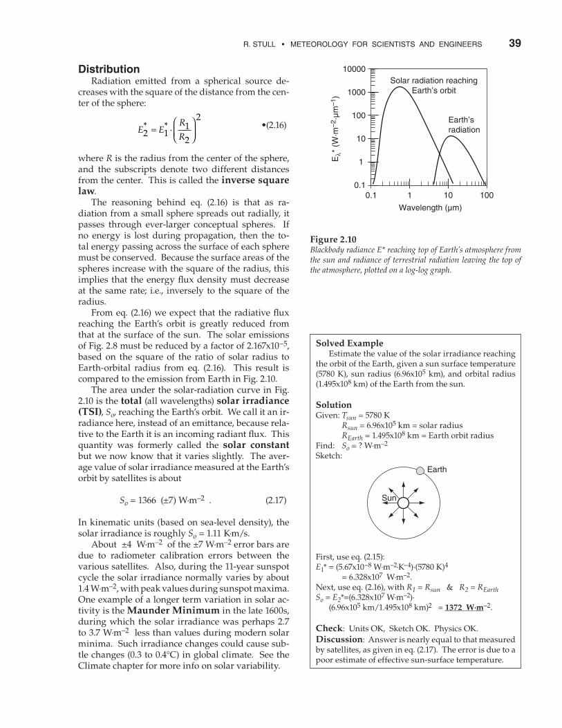
where R is the radius from the center of the sphere, and the subscripts denote two different distances from the center. This is called the inverse square law. The reasoning behind eq. (2.16) is that as ra-diation from a small sphere spreads out radially, it passes through ever-larger conceptual spheres. If no energy is lost during propagation, then the to-tal energy passing across the surface of each sphere must be conserved. Because the surface areas of the spheres increase with the square of the radius, this implies that the energy flux density must decrease at the same rate; i.e., inversely to the square of the radius. From eq. (2.16) we expect that the radiative flux reaching the Earth’s orbit is greatly reduced from that at the surface of the sun. The solar emissions of Fig. 2.8 must be reduced by a factor of 2.167x10–5, based on the square of the ratio of solar radius to Earth-orbital radius from eq. (2.16). This result is compared to the emission from Earth in Fig. 2.10. The area under the solar-radiation curve in Fig. 2.10 is the total (all wavelengths) solar irradiance (TSI), So, reaching the Earth’s orbit. We call it an ir-radiance here, instead of an emittance, because rela-tive to the Earth it is an incoming radiant flux. This quantity was formerly called the solar constant but we now know that it varies slightly. The aver-age value of solar irradiance measured at the Earth’s orbit by satellites is about

So = 1366 (±7) W·m–2 . (2.17)

In kinematic units (based on sea-level density), the solar irradiance is roughly So = 1.11 K·m/s. About ±4 W·m–2 of the ±7 W·m–2 error bars are due to radiometer calibration errors between the various satellites. Also, during the 11-year sunspot cycle the solar irradiance normally varies by about 1.4 W·m–2, with peak values during sunspot maxima. One example of a longer term variation in solar ac-tivity is the Maunder Minimum in the late 1600s, during which the solar irradiance was perhaps 2.7 to 3.7 W·m–2 less than values during modern solar minima. Such irradiance changes could cause sub-tle changes (0.3 to 0.4°C) in global climate. See the Climate chapter for more info on solar variability.

Figure 2.10Blackbody radiance E* reaching top of Earth’s atmosphere from the sun and radiance of terrestrial radiation leaving the top of the atmosphere, plotted on a log-log graph.

Solved Example Estimate the value of the solar irradiance reaching the orbit of the Earth, given a sun surface temperature (5780 K), sun radius (6.96x105 km), and orbital radius (1.495x108 km) of the Earth from the sun.

SolutionGiven: Tsun = 5780 K Rsun = 6.96x105 km = solar radius REarth = 1.495x108 km = Earth orbit radiusFind: So = ? W·m–2 Sketch:

First, use eq. (2.15):E1* = (5.67x10–8 W·m–2·K–4)·(5780 K)4 = 6.328x107 W·m–2.Next, use eq. (2.16), with R1 = Rsun & R2 = REarth So = E2*=(6.328x107 W·m–2)· (6.96x105 km/1.495x108 km)2 = 1372 W·m–2.

Check: Units OK, Sketch OK. Physics OK.Discussion: Answer is nearly equal to that measured by satellites, as given in eq. (2.17). The error is due to a poor estimate of effective sun-surface temperature.


According to the inverse-square law, variations of distance between Earth and sun cause changes of the solar radiative forcing, S, that reaches the top of the atmosphere:

S SoRR

=

·2

(2.18)

where So = 1366 W·m–2 is the average total solar ir-radiance measured at an average distance R = 149.6 Gm between the sun and Earth, and R is the actual distance between Earth and the sun as given by eq. (2.4). Remember that the solar irradiance and the solar radiative forcing are the fluxes across a surface that is perpendicular to the solar beam, measured above the Earth’s atmosphere. Let irradiance E be any radiative flux crossing a unit area that is perpendicular to the path of the radiation. If this radiation strikes a surface that is not perpendicular to the radiation, then the radia-tion per unit surface area is reduced according to the sine law. The resulting flux, Frad, at this surface is:

Frad E= · sin( )Ψ (2.19)

where Ψ is the elevation angle (the angle of the sun above the surface). In kinematic form, this is

F

ECrad

p=

ρ·· sin( )Ψ

•(2.20)

where ρ·Cp is given under eq. (2.11).

average daily insolation The acronym “insolation” means “incoming solar radiation” at the top of the atmosphere. The average daily insolation E takes into account both the solar elevation angle (which varies with season and time of day) and the duration of daylight. For example, there is more total insolation at the poles in summer than at the equator, because the low sun angle near the poles is more than compensated by the long periods of daylight.

(2.21)

E

So aR

ho s=π

′ +

· · ·sin( )·sin( )

cos(

2φ δ

φ))·cos( )·sin( )δs ho

where So =1366 W/m2 is the solar irradiance, a = 149.457 Gm is Earth’s semi-major axis length, R is the actual distance for any day of the year, from eq.

Solved Example(§) Using the results from an earlier solved example that calculated the true anomaly and sun-Earth dis-tance for several days during the year, find the solar radiative forcing for those days.

SolutionGiven: R values from previously solved exampleFind: S = ? W·m–2

Sketch: (same as Fig 2.2)Use eq. (2.18).

Date d R(ν) (Gm)

S(W/m2)

4 Jan 4 146.96 141818 Jan 18 147.04 14161 Feb 32 147.25 141215 Feb 46 147.60 14051 Mar 60 148.06 139715 Mar 74 148.60 138629 Mar 88 149.18 137612 Apr 102 149.78 136526 Apr 116 150.36 135421 Jun 172 151.88 132723 Sep 266 150.01 136122 Dec 356 147.03 1416

Check: Units OK. Physics OK.Discussion: During N. Hemisphere winter, solar ra-diative forcing is up to 50 W·m–2 larger than average.

Solved Example During the equinox at noon at latitude ϕ =60°, the solar elevation angle is Ψ = 90° – 60° = 30°. If the at-mosphere is perfectly transparent, then how much ra-diative flux is absorbed into a perfectly black asphalt parking lot?

SolutionGiven: Ψ = 30° = elevation angle E = So = 1366 W·m–2. solar irradianceFind: Frad = ? W·m–2 Sketch:

Use eq. (2.19): Frad = (1366 W·m–2)·sin(30°) = 683 W·m–2.

Check: Units OK. Sketch OK. Physics OK.Discussion: Because the solar radiation is striking the parking lot at an angle, the radiative flux into the parking lot is half of the solar irradiance.


(2.4). In eq. (2.21), ho’ is the sunset and sunrise hour angle in radians. The hour angle ho at sunrise and sunset can be found using the following steps:

α φ δ= − tan( )·tan( )s (2.22a)

β α= −min[ , (max( , )]1 1 (2.22b)

ho = arccos( )β (2.22c)

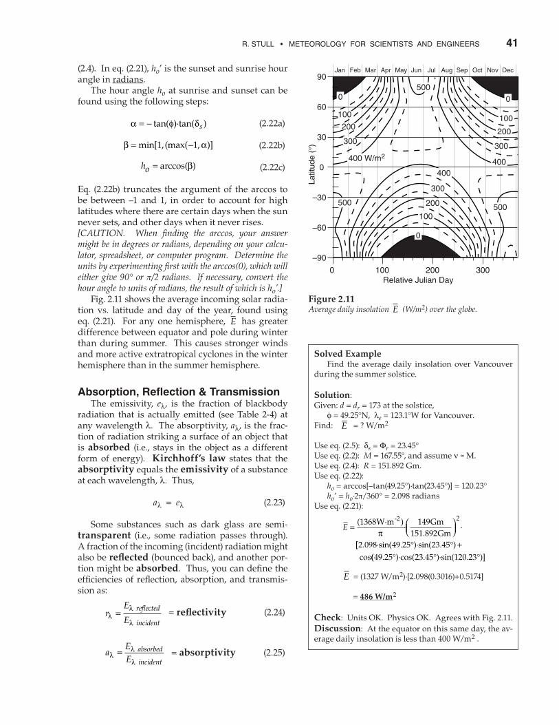
Eq. (2.22b) truncates the argument of the arccos to be between –1 and 1, in order to account for high latitudes where there are certain days when the sun never sets, and other days when it never rises.[CAUTION. When finding the arccos, your answer might be in degrees or radians, depending on your calcu-lator, spreadsheet, or computer program. Determine the units by experimenting first with the arccos(0), which will either give 90° or π/2 radians. If necessary, convert the hour angle to units of radians, the result of which is ho’.] Fig. 2.11 shows the average incoming solar radia-tion vs. latitude and day of the year, found using eq. (2.21). For any one hemisphere, E has greater difference between equator and pole during winter than during summer. This causes stronger winds and more active extratropical cyclones in the winter hemisphere than in the summer hemisphere.

absorption, reflection & transmission The emissivity, eλ, is the fraction of blackbody radiation that is actually emitted (see Table 2-4) at any wavelength λ. The absorptivity, aλ, is the frac-tion of radiation striking a surface of an object that is absorbed (i.e., stays in the object as a different form of energy). Kirchhoff’s law states that the absorptivity equals the emissivity of a substance at each wavelength, λ. Thus,

aλ = eλ (2.23)

Some substances such as dark glass are semi-transparent (i.e., some radiation passes through). A fraction of the incoming (incident) radiation might also be reflected (bounced back), and another por-tion might be absorbed. Thus, you can define the efficiencies of reflection, absorption, and transmis-sion as:

rE

Ereflected

incidentλ

λ

λ=

= reflectivity (2.24)

aEE

absorbed

incidentλ

λ

λ=

= absorptivity (2.25)

Solved Example Find the average daily insolation over Vancouver during the summer solstice.

Solution: Given: d = dr = 173 at the solstice, ϕ = 49.25°N, λe = 123.1°W for Vancouver.Find: E = ? W/m2

Use eq. (2.5): δs = Φr = 23.45°Use eq. (2.2): M = 167.55°, and assume ν ≈ M.Use eq. (2.4): R = 151.892 Gm. Use eq. (2.22): ho = arccos[–tan(49.25°)·tan(23.45°)] = 120.23° ho’ = ho·2π/360° = 2.098 radiansUse eq. (2.21):

E =

( )·

.·

1368 149151 892

2W·m GmGm

-2

π[[ . ·sin( . )·sin( . )

cos2 098 49 25 23 45° ° +

(( . )·cos( . )·sin( . )]49 25 23 45 120 23° ° °

E = (1327 W/m2)·[2.098(0.3016)+0.5174]

= 486 W/m2

Check: Units OK. Physics OK. Agrees with Fig. 2.11.Discussion: At the equator on this same day, the av-erage daily insolation is less than 400 W/m2 .

Figure 2.11Average daily insolation E (W/m2) over the globe.


tE

Etransmitted

incidentλ

λ

λ=

= transmissivity (2.26)

Values of eλ, aλ, rλ, and tλ are between 0 and 1. The sum of the last three fractions must total 1, as 100% of the radiation at any wavelength must be accounted for:

1 = + +a r tλ λ λ (2.27)or (2.28) Eλ incoming = Eλ absorbed +Eλ reflected +Eλ transmitted

For opaque (tλ = 0) substances such as the Earth’s surface, you find: aλ = 1 – rλ. The reflectivity, absorptivity, and transmissivity usually vary with wavelength. For example, clean snow reflects about 90% of incoming solar radiation, but reflects almost 0% of IR radiation. Thus, snow is “white” in visible light, and “black” in IR. Such behavior is crucial to surface temperature forecasts. Instead of considering a single wavelength, it is also possible to examine the net effect over a range of wavelengths. The ratio of total reflected to total incoming solar radiation (i.e., averaged over all solar wavelengths) is called the albedo, A :

AE

Ereflected

incoming= •(2.29)

The average global albedo for solar radiation reflect-ed from Earth is A = 30% (see the Climate chapter). The actual global albedo at any instant varies with ice cover, snow cover, cloud cover, soil moisture, to-pography, and vegetation (Table 2-5). The Moon’s albedo is only 7%. The surface of the Earth (land and sea) is a very strong absorber and emitter of radiation.

Table 2-5. Typical albedos (%) for sunlight.

Surface A (%) Surface A (%)alfalfa 23-32 forest, decid. 10-25buildings 9 granite 12-18clay, wet 16 grass, green 26clay, dry 23 gypsum 55cloud, thick 70-95 ice, gray 60cloud, thin 20-65 lava 10concrete 15-37 lime 45corn 18 loam, wet 16cotton 20-22 loam, dry 23field, fallow 5-12 meadow, green 10-20forest, conif. 5-15 potatoes 19

Table 2-4. Typical infrared emissivities.

Surface e Surface ealfalfa 0.95 iron, galvan. 0.13-0.28aluminum 0.01-0.05 leaf 0.8 µm 0.05-0.53asphalt 0.95 leaf 1 µm 0.05-0.6bricks, red 0.92 leaf 2.4 µm 0.7-0.97cloud, cirrus 0.3 leaf 10 µm 0.97-0.98cloud, alto 0.9 lumber, oak 0.9cloud, low 1.0 paper 0.89-0.95concrete 0.71-0.9 plaster, white 0.91desert 0.84-0.91 sand, wet 0.98forest, conif. 0.97 sandstone 0.98forest, decid. 0.95 shrubs 0.9glass 0.87-0.94 silver 0.02grass 0.9-0.95 snow, fresh 0.99grass lawn 0.97 snow, old 0.82gravel 0.92 soils 0.9-0.98human skin 0.95 soil, peat 0.97-0.98ice 0.96 urban 0.85-0.95

Solved Example If 500 W/m2 of visible light strikes a translucent object that allows 100 W/m2 to shine through and 150 W/m2 to bounce off, find the transmissivity, reflectiv-ity, absorptivity, and emissivity.

SolutionGiven: Eλ incoming = 500 W/m2 , Eλ transmitted = 100 W/m2 , Eλ reflected = 150 W/m2

Find: aλ = ? , eλ = ? , rλ = ? , and tλ = ?

Use eq. (2.26): tλ = (100 W/m2) / (500 W/m2) = 0.2 Use eq. (2.24): rλ = (150 W/m2) / (500 W/m2) = 0.3 Use eq. (2.27): aλ = 1 – 0.2 – 0.3 = 0.5 Use eq. (2.23): eλ = aλ = 0.5

Check: Units dimensionless. Physics reasonable.Discussion: By definition, translucent means part-ly transparent, and partly absorbing.

Table 2-5 (continuation). Typical albedos (%).

Surface A (%) Surface A (%)rice paddy 12 soil, red 17road, asphalt 5-15 soil, sandy 20-25road, dirt 18-35 sorghum 20rye winter 18-23 steppe 20sand dune 20-45 stones 20-30savanna 15 sugar cane 15snow, fresh 75-95 tobacco 19snow, old 35-70 tundra 15-20soil, dark wet 6-8 urban, mean 15soil, light dry 16-18 water, deep 5-20soil, peat 5-15 wheat 10-23


Within the air, however, the process is a bit more complicated. One approach is to treat the whole at-mospheric thickness as a single object. Namely, you can compare the radiation at the top versus bottom of the atmosphere to examine the total emissivity, ab-sorptivity, and reflectivity of the whole atmosphere. Over some wavelengths called windows there is little absorption, allowing the radiation to “shine” through. In other wavelength ranges there is partial or total absorption. Thus, the atmosphere acts as a filter. Atmospheric windows and transmissivity are discussed in detail in the Remote Sensing and Cli-mate chapters.

beer’s law Sometimes you must examine radiative extinc-tion (reduction of radiative flux) across a short path length ∆s within the atmosphere (Fig. 2.12). Let n be the number density of radiatively important parti-cles in the air (particles/m3), and b be the extinction cross section of each particle (m2/particle), where this latter quantity gives the area of the shadow cast by each particle. Extinction can be caused by absorption and scat-tering of radiation. If the change in radiation is due only to absorption, then the absorptivity across this layer is

aE E

Eincident transmitted

incident=

− (2.30)

Beer’s law gives the relationship between inci-dent radiative flux, Eincident, and transmitted radia-tive flux, Etransmitted, as

E Etransmitted incidentn b s= − ∆· · ·e (2.31a)

Beer’s law can be written using an extinction coef-ficient, k: E Etransmitted incident

k s= − ∆· · ·e ρ (2.31b)

where ρ is the density of air, and k has units of m2/gair . The total extinction across the whole path can be quantified by a dimensionless optical thick-ness (or optical depth in the vertical), τ , allowing Beer’s law to be rewritten as: E E etransmitted incident= −· τ (2.31c)

To simplify these equations, sometimes a volume extinction coefficient γ is defined by

γ = n·b = k·ρ (2.32)

Visual range (V, one definition of visibility) is the distance where the intensity of transmitted light has decreased to 2% of the incident light. It estimates the max distance ∆s (km) you can see through air.

Solved Example Suppose that soot from a burning automobile tire has number density n = 107 m–3, and an extinction cross section of b = 10–9 m2. (a) Find the radiative flux that was not attenuated (i.e., reduction from the solar constant) across the 20 m diameter smoke plume. As-sume the incident flux equals the solar constant. (b) Find the optical depth. (c) If this soot fills the air, what is the visual range?

SolutionGiven: n = 107 m–3 , b = 10–9 m2 , ∆s = 20 m Eincident = S = 1366 W·m–2 solar constantFind: Etran =? W·m–2, τ =? (dimensionless), V =? kmSketch:

Use eq. (2.32): γ = (107 m–3)·(10–9 m2) = 0.01 m–1

(a) Use eq. (2.31a)Etran = 1366 W·m–2 · exp[ –(0.01 m–1)·(20 m)] = 1366 W·m–2 · exp[–0.2] = 1118 W·m–2

(b) Rearrange eq. (2.31c): τ = ln(Ein/Etransmitted) = ln(1366/1118) = 0.20

(c) Rearrange eq. (2.31a): ∆s = [ln(Eincident/Etrans)]/γ . V = ∆s = [ln(1/0.02)]/0.01 m–1 = 0.391 km

Check: Units OK. Sketch OK. Physics OK.Discussion: Not much attenuation through this small smoke plume; namely, 1366 – 1118 = 248 W·m–2 was absorbed by the smoke. However, if this smoke fills the air, then visibility is very poor.

Figure 2.12Reduction of radiation across an air path due to absorption and scattering by particles such as air-pollution aerosols or cloud droplets, illustrating Beer’s law.


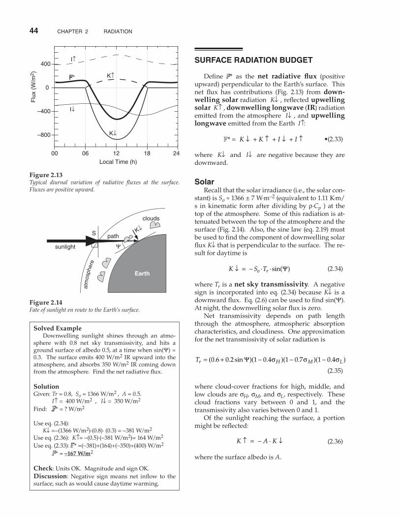
surFaCe radiation budGet

Define F* as the net radiative flux (positive upward) perpendicular to the Earth’s surface. This net flux has contributions (Fig. 2.13) from down-welling solar radiation K↓ , reflected upwelling solar K↑ , downwelling longwave (IR) radiation emitted from the atmosphere I↓ , and upwelling longwave emitted from the Earth I↑:

F* = ↓ + ↑ + ↓ + ↑K K I I •(2.33)

where K↓ and I↓ are negative because they are downward.

solar Recall that the solar irradiance (i.e., the solar con-stant) is So ≈ 1366 ± 7 W·m–2 (equivalent to 1.11 K·m/s in kinematic form after dividing by ρ·Cp ) at the top of the atmosphere. Some of this radiation is at-tenuated between the top of the atmosphere and the surface (Fig. 2.14). Also, the sine law (eq. 2.19) must be used to find the component of downwelling solar flux K↓ that is perpendicular to the surface. The re-sult for daytime is

K S To r↓ = − · ·sin( )Ψ (2.34)

where Tr is a net sky transmissivity. A negative sign is incorporated into eq. (2.34) because K↓ is a downward flux. Eq. (2.6) can be used to find sin(Ψ). At night, the downwelling solar flux is zero. Net transmissivity depends on path length through the atmosphere, atmospheric absorption characteristics, and cloudiness. One approximation for the net transmissivity of solar radiation is

Tr H M L= + − − −( . . sin )( . )( . )( . )0 6 0 2 1 0 4 1 0 7 1 0 4Ψ σ σ σ

(2.35)

where cloud-cover fractions for high, middle, and low clouds are σH, σM, and σL, respectively. These cloud fractions vary between 0 and 1, and the transmissivity also varies between 0 and 1. Of the sunlight reaching the surface, a portion might be reflected:

K A K↑ = − ↓· (2.36)

where the surface albedo is A.

Figure 2.14Fate of sunlight en route to the Earth’s surface.

Solved Example Downwelling sunlight shines through an atmo-sphere with 0.8 net sky transmissivity, and hits a ground surface of albedo 0.5, at a time when sin(Ψ) = 0.3. The surface emits 400 W/m2 IR upward into the atmosphere, and absorbs 350 W/m2 IR coming down from the atmosphere. Find the net radiative flux.

SolutionGiven: Tr = 0.8, So = 1366 W/m2 , A = 0.5. I↑ = 400 W/m2 , I↓ = 350 W/m2 Find: F* = ? W/m2

Use eq. (2.34): K↓ =–(1366 W/m2)·(0.8)· (0.3) = –381 W/m2 Use eq. (2.36): K↑= –(0.5)·(–381 W/m2)= 164 W/m2 Use eq. (2.33): F* =(–381)+(164)+(–350)+(400) W/m2 F* = –167 W/m2

Check: Units OK. Magnitude and sign OK.Discussion: Negative sign means net inflow to the surface, such as would cause daytime warming.

Figure 2.13Typical diurnal variation of radiative fluxes at the surface. Fluxes are positive upward.


longwave (ir) Upward emission of IR radiation from the Earth’s surface can be found from the Stefan-Boltzmann re-lationship:

I e TIR SB↑= · ·σ 4 (2.37)

where eIR is the surface emissivity in the IR por-tion of the spectrum (eIR = 0.9 to 0.99 for most sur-faces), and σSB is the Stefan-Boltzmann constant (= 5.67x10–8 W·m–2·K–4). However, downward IR radiation from the at-mosphere is much more difficult to calculate. As an alternative, sometimes a net longwave flux is de-fined by

I I I* = ↓ + ↑ (2.38)

One approximation for this flux is

I b H M L* ·( . . . )= − − −1 0 1 0 3 0 6σ σ σ (2.39)

where parameter b = 98.5 W·m–2 , or b = 0.08 K·m·s–1 in kinematic units.

net radiation Combining eqs. (2.33), (2.34), (2.35), (2.36) and (2.39) gives the net radiation (F*, defined positive upward):

F * ( )· · · sin( ) *= − − +1 A S T Ir Ψ daytime •(2.40a)

= I* nighttime •(2.40b)

aCtinoMeters

Sensors designed to measure electromagnetic radiative flux are generically called actinometers or radiometers. In meteorology, actinometers are usually oriented to measure downwelling or up-welling radiation. Sensors that measure the differ-ence between down- and up-welling radiation are called net actinometers. Special categories of actinometers are designed to measure different wavelength bands:

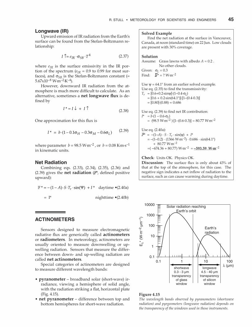
• pyranometer – broadband solar (short-wave) ir-radiance, viewing a hemisphere of solid angle, with the radiation striking a flat, horizontal plate (Fig. 4.15).

• net pyranometer – difference between top and bottom hemispheres for short-wave radiation.

Solved Example Find the net radiation at the surface in Vancouver, Canada, at noon (standard time) on 22 Jun. Low clouds are present with 30% coverage.

SolutionAssume: Grass lawns with albedo A = 0.2 . No other clouds.Given: σL = 0.3Find: F* = ? W·m–2

Use ψ = 64.1° from an earlier solved example.Use eq. (2.35) to find the transmissivity:Tr = [0.6+0.2·sinψ]·(1–0.4·σL) = [0.6 + 0.2·sin(64.1°)]·[1–(0.4·0.3)] = [0.80]·(0.88) = 0.686

Use eq. (2.39) to find net IR contribution:I* = b·(1 – 0.6·σL) = (98.5 W·m–2 )·[1–(0.6·0.3)] = 80.77 W·m–2

Use eq. (2.40a): F* = –(1–A) · S · Tr · sin(ψ) + I* = –(1–0.2) · (1366 W·m–2) · 0.686 · sin(64.1°) + 80.77 W·m–2 =( –674.36 + 80.77) W·m–2 = –593.59 W·m–2

Check: Units OK. Physics OK.Discussion: The surface flux is only about 43% of that at the top of the atmosphere, for this case. The negative sign indicates a net inflow of radiation to the surface, such as can cause warming during daytime.

Figure 4.15The wavelength bands observed by pyranometers (shortwave radiation) and pyrgeometers (longwave radiation) depends on the transparency of the windows used in those instruments.


• pyrheliometer – solar (short wave) direct-beam radiation normal to a flat surface (and shielded from diffuse radiation).

• diffusometer – a pyranometer that measures only diffuse solar radiation scattered from air, particles, and clouds in the sky, by using a device that shades the sensor from direct sunlight.

• pyrgeometer – infrared (long-wave) radiation from a hemisphere that strikes a flat, horizontal surface (Fig. 4.15).

• net pyrgeometer – difference between top and bottom hemispheres for infrared (long-wave) ra-diation.

• radiometer – measure all wavelengths of radia-tion (short, long, and other bands).

• net radiometer – difference between top and bot-tom hemispheres of radiation at all wavelengths.

• spectrometers – measures radiation as a func-tion of wavelength, to determine the spectrum of radiation.

Inside many radiation sensors is a bolometer, which works as follows. Radiation strikes an object such as a metal plate, the surface of which has a coat-ing that absorbs radiation mostly in the wavelength band to be measured. By measuring the tempera-ture of the radiatively heated plate relative to a non-irradiated reference, the radiation intensity can be inferred for that wavelength band. The metal plate is usually enclosed in a glass or plastic hemispheric chamber to reduce error caused by heat conduction with the surrounding air. Inside other radiation sensors are photometers. Some photometers use the photoelectric effect, where certain materials release electrons when struck by electromagnetic radiation. One type of photometer uses photovoltaic cells (also called solar cells), where the amount of electrical energy generated can be related to the incident radiation. Another photometric method uses photoresistor, which is a high-resistance semiconductor that be-comes more conductive when irradiated by light. Other photometers use charge-coupled devic-es (CCDs) similar to the image sensors in digital cameras. These are semiconductor integrated cir-cuits with an array of tiny capacitors that can gain their initial charge by the photoelectric effect, and can then transfer their charge to neighboring capaci-tors to eventually be “read” by the surrounding cir-cuits. Simple spectrometers use different filters in front of bolometers or photometers to measure narrow wavelength bands. Higher spectral-resolution spec-trometers use interferometry (similar to the Mi-chelson inteferometer described in physics books), where the fringes of an interference pattern can be

on doinG sCienCe • seek solutions

Most differential equations describing meteo-rological phenomena cannot be solved analytically. They cannot be integrated; they do not appear in a table of integrals; and they are not covered by the handful of mathematical tricks that you learned in math class. But there is nothing magical about an analytical solution. Any reasonable solution is better than no solution. Be creative. While thinking of creative solutions, also think of ways to check your answer. Is it the right order of magnitude, right sign, right units, does it approach a known answer in some limit, must it satisfy some other physical constraint or law or budget?

Example Find the irradiance that can pass through an atmo-spheric “window” between wavelengths λ1 and λ2.

Solution: Approach: Integrate Planck’s law between the specified wavelengths. This is the area under a por-tion of the Planck curve.

Check: The area under the whole spectral curve should yield the Stefan-Boltzmann (SB) law. Namely, the answer should be smaller than the SB answer, but should increase and converge to the SB answer as the lower and upper λ limits approach 0 and ∞, respec-tively.

Methods:• Pay someone else to get the answer (Don’t do this in school!), but be sure to check it yourself.• Look up the answer in a Table of Integrals.• Integrate it using the tricks you learned in math class.• Integrate it using a symbolic equation solver on a computer, such as Mathematica or Maple.• Find an approximate solution to the full equation. For example, integrate it numerically on a computer. (Trapezoid method, Gaussian integration, finite dif-ference iteration, etc.)• Find an exact solution for an approximation to the eq., such as a model or idealization of the physics. Most eqs. in this textbook have used this approach.• Draw the Planck curve on graph paper. Count the squares under the curve between the wavelength bands, and compare to the value of each square, or to the area under the whole curve. (We will use this ap-proach extensively in the Thunderstorm chapter.)• Draw the curve, and measure area with a planim-eter.• Draw the Planck curve on cardboard or thick pa-per. Cut out the whole area under the curve. Weigh it. Then cut the portion between wavelengths, & weigh again.• ...and there are probably many more methods.


measured and related to the spectral intensities. These are also sometimes called Fourier-trans-form spectrometers, because of the mathematics used to extract the spectral information from the spacing of the fringes. You can learn more about radiation, including the radiative transfer equation, in the weather-satel-lite section of the Remote Sensing chapter. Satellites use radiometers and spectrometers to remotely ob-serve the Earth-atmosphere system. Other satellite-borne radiometers are used to measure the global radiation budget (see the Climate chapter).

suMMarY

The variations of temperature and humidity that you feel near the ground are driven by the diurnal cycle of solar heating during the day and infrared cooling at night. Both diurnal and seasonal heating cycles can be determined from the geometry of the Earth’s rotation and orbit around the sun. The same orbital mechanics describes weather-satellite orbits, as is discussed in the Remote Sensing chapter. Short-wave radiation is emitted from the sun and propagates through space. It illuminates a hemi-sphere of Earth. The portion of this radiation that is absorbed is the heat input to the Earth-atmosphere system that drives Earth’s weather. IR radiation from the atmosphere is absorbed at the ground, and IR radiation is also emitted from the ground. The IR and short-wave radiative fluxes do not balance, leaving a net radiation term acting on the surface. Instruments to measure radiation are called ac-tinometers or radiometers. Radiometers and spec-trometers can be used in remote sensors such as weather satellites.

threads Just a reminder that the “threads” section at the end of each chapter is designed to highlight linkag-es to material in the other chapters. It is included to help you develop a coherent picture of atmospheric science, and to anticipate your question of “Why is this material important?”. Radiation affects motions on a wide range of scales, and it affects thermodynamics. Excess solar radiation near the equator, and excess IR cooling at the poles is the driving force for the global circula-tion (Chapter 11). It ultimately creates the synoptic weather patterns of high and low pressure systems and fronts (Chapter 12 and 13). Averaged over the

whole globe, it controls the Earth’s climate (Chapter 21). Radiative heating at different heights creates a vertical atmospheric structure quantified by a stan-dard atmosphere (Chapter 1), and affects static sta-bility and cloud growth (Chapters 5 and 6). On a smaller scale, IR radiative cooling drives downslope drainage winds at night (Chapter 17). Also, sun-light interacts with ice crystals and raindrops to cre-ate beautiful optical phenomena such as rainbows (Chapter 22). Planck’s law shows the peak wavelength of solar emissions to be in the visible portion of the spectrum. Sunlight drives the diurnal cycle of the surface heat budget described in Chapter 3, which mostly affects air near the ground, in the atmospheric boundary layer (Chapter 18). Orbital mechanics dictates the optimum weather satellite altitudes for observing such storms (Chap-ter 8).

exerCises

numerical problems(Students, don’t forget to put a box around each an-swer.)

N1. Given distances R between the sun and planets compute the orbital periods (Y) of: a. Mercury (R = 58 Gm) b. Venus (R = 108 Gm) c. Mars (R = 228 Gm) d. Jupiter (R = 778 Gm) e. Saturn (R = 1,427 Gm) f. Uranus (R = 2,869 Gm) g. Neptune (R = 4,498 Gm) h. Pluto (R = 5,900 Gm) i. Eris: given Y = 557 Earth years, estimate the distance R from the sun assuming a circular orbit. (Note: Eris’ orbit is highly eccentric and steeply tilt-ed at 44° relative to the plane of the rest of the solar system, so our assumption of a circular orbit was made here only to simplify the exercise.)

N2. This year, what is the date and time of the: a. perihelion b. vernal equinox c. summer solstice d. aphelion e. autumnal equinox f. winter solstice

N3. What is the relative Julian day for: a. 10 Jan b. 25 Jan c. 10 Feb d. 25 Feb e. 10 Mar f. 25 Mar g. 10 Apr h. 25 Apr i. 10 May j. 25 May k. 10 Jun l. 25 Jun


a. Arctic Circle b. 75°N c. 85°N d. North Pole e. Antarctic Circle f. 70°S g. 80°S h. South Polefor each of the following dates: (i) 22 Dec (ii) 23 Mar (iii) 22 Jun

N9(§). Plot the duration of evening civil twilight (dif-ference between end of twilight and sunset times) vs. latitude between the south and north poles, for the following date: a. 22 Dec b. 5 Feb c. 21 Mar d. 5 May e. 21 Jun f. 5 Aug g. 23 Sep h. 5 Nov

N10. On 15 March for the city listed from exercise N5, at what local standard time is: a. geometric sunrise b. apparent sunrise c. start of civil twilight d. start of military twilight e. start of astronomical twilight f. geometric sunset g. apparent sunset h. end of civil twilight i. end of military twilight j. end of astronomical twilight

N11. Calculate the Eq. of Time correction for: a. 1 Jan b. 15 Jan c. 1 Feb d. 15 Feb e. 1 Mar f. 15 Mar g. 1 Apr h. 15 Apr i. 1 May j. 15 May

N12. Find the mass flux (kg·m–2·s–1) at sea-level, giv-en a kinematic mass flux (m/s) of: a. 2 b. 5 c. 7 d. 10 e. 14 f. 18 g. 21 h. 25 i. 30 j. 33 k. 47 l. 59 m. 62 n. 75

N13. Find the kinematic heat fluxes at sea level, giv-en these regular fluxes (W·m–2): a. 1000 b. 900 c. 800 d. 700 e. 600 f. 500 g. 400 h. 300 i. 200 j. 100 k. 43 l. –50 m. –250 n. –325 o. –533

N14. Find the frequency, circular frequency, and wavenumber for light of color: a. red b. orange c. yellow d. green e. cyan f. blue f. indigo g. violet

N15(§). Plot Planck curves for the following black-body temperatures (K): a. 6000 b. 5000 c. 4000 d. 3000 e. 2500 f. 2000 g. 1500 h. 1000 i. 750 j. 500 k. 300 l. 273 m. 260 n. 250 h. 240

N16. For the temperature of exercise N15, find: (i) wavelength of peak emissions (ii) total emittance (i.e., total amount of emis-sions)

m. 10 Jul n. 25 Jul o. 10 Aug p. 25 Aug q. 10 Sep r. 25 Sep s. 10 Oct t. 25 Oct u. 10 Nov v. 25 Nov w. 10 Dec x. 25 Dec y. today’s date z. date assigned by instructor

N4. For the date assigned from exercise N3, find: (i) mean anomaly (ii) true anomaly (iii) distance between the sun and the Earth (iv) solar declination angle (v) average daily insolation

N5(§). Plot the local solar elevation angle vs. local time for 22 December, 23 March, and 22 June for the following city: a. Seattle, WA, USA b. Corvallis, OR, USA c. Boulder, CO, USA d. Norman, OK, USA e. Madison, WI, USA f. Toronto, Canada g. Montreal, Canada h. Boston, MA, USA i. New York City, NY, USA j. University Park, PA, USA k. Princeton, NJ, USA l. Washington, DC, USA m. Raleigh, NC, USA n. Tallahassee, FL, USA o. Reading, England p. Toulouse, France q. München, Germany r. Bergen, Norway s. Uppsala, Sweden t. DeBilt, The Netherlands u. Paris, France v. Tokyo, Japan w. Beijing, China x. Warsaw, Poland y. Madrid, Spain z. Melbourne, Australia aa. Your location today. bb. A location assigned by your instructor

N6(§). Plot the local solar azimuth angle vs. local time for 22 December, 23 March, and 22 June, for the location from exercise N5.

N7(§). Plot the local solar elevation angle vs. azi-muth angle (similar to Fig. 2.6) for the location from exercise N5. Be sure to add tic marks along the re-sulting curve and label them with the local standard times.

N8(§). Plot local solar elevation angle vs. azimuth angle (such as in Fig. 2.6) for the following location:


N17. Estimate the value of solar irradiance reaching the orbit of the planet from exercise N1.

N18(§). a. Plot the value of solar irradiance reaching Earth’s orbit as a function of relative Julian day. b. Using the average solar irradiance, plot the ra-diative flux (reaching the Earth’s surface through a perfectly clear atmosphere) vs. latitude. Assume lo-cal noon.

N19(§). For the city of exercise N1, plot the average daily insolation vs. Julian day.

N20. What is the value of IR absorptivity of: a. aluminum b. asphalt c. cirrus cloud d. conifer forest e. grass lawn f. ice g. oak h. silver i. old snow j. urban average k. concrete average l. desert average m. shrubs n. soils average

N21. Suppose polluted air reflects 30% of the incom-ing solar radiation. How much (W/m2) is absorbed, emitted, reflected, and transmitted? Assume an in-cident radiative flux equal to the solar irradiance, given a transmissivity of: a. 0 b. 0.05 c. 0.1 d. 0.15 e. 0.2 f. 0.25 g. 0.3 h. 0.35 i. 0.4 j. 0.45 k. 0.5 l. 0.55 m. 0.6 n. 0.65 o. 0.7

N22. What is the value of albedo for the following land use? a. buildings b. dry clay c. corn d. green grass e. ice f. potatoes g. rice paddy h. savanna i. red soil j. sorghum k. sugar cane l. tobacco

N23. What product of number density times absorp-tion cross section is needed in order for 50% of the incident radiation to be absorbed by airborne volca-nic ash over the following path length (km)? a. 0.2 b. 0.4 c. 0.6 d. 0.8 e. 1.0 f. 1.5 g. 2 h. 2.5 i. 3 j. 3.5 k. 4 l. 4.5 m. 5 n. 7

N24. What fraction of incident radiation is transmit-ted through a volcanic ash cloud of optical depth: a. 0.2 b. 0.5 c. 0.7 d. 1.0 e. 1.5 f. 2 g. 3 h. 4 j. 5 k. 6 l. 7 m. 10 n. 15 o. 20

N25. What is the visual range (km) for polluted air that has volume extinction coefficient (m-1) of: a. 0.00001 b. 0.00002 c. 0.00005 d. 0.0001 e. 0.0002 f. 0.0005 g. 0.001 h. 0.002 i. 0.005 j. 0.01 k. 0.02 l. 0.05

N26. (i) What is the value of solar downward direct radiative flux reaching the surface at the city from

exercise N5 at noon on 4 July, given 20% coverage of cumulus (low) clouds. (ii) If the albedo is 0.5 in your town, what is the reflected solar flux at that same time? (iii) What is the approximate value of net longwave radiation at that time? (iv) What is the net radiation at that time, given all the info from parts (i) - (iii)?

N27. For a surface temperature of 20°C, find the emitted upwelling IR radiation (W/m2) over the sur-face-type from exercise N20.

understanding & Critical evaluationU1. At what time of year does the true anomaly equal: a. 45° b. 90° c. 135° d. 180° e. 225° f. 270° g. 315° h. 360°

U2(§) a. Calculate and plot the position (true anom-aly and distance) of the Earth around the sun for the first day of each month. b. Verify Kepler’s second law. c. Compare the elliptical orbit to a circular orbit.

U3. What is the optimum angle for solar collectors at your town?

U4. Design a device to measure the angular diam-eter of the sun when viewed from Earth. (Hint, one approach is to allow the sun to shine through a pin hole on to a flat surface. Then measure the width of the projected image of the sun on this surface di-vided by the distance between the surface and the pin hole. What could cause errors in this device?)

U5. For your city, plot the azimuth angle for appar-ent sunrise vs. relative Julian day. This is the direc-tion you need to point your camera if your want to photograph the sunrise.

U6. a. Compare the length of daylight in Fairbanks, AK, vs Miami, FL, USA. b. Why do vegetables grow so large in Alaska? c. Why are few fruits grown in Alaska?

U7. How would Fig. 2.6 be different if daylight (summer) time were used in place of standard time during the appropriate months?

U8(§). Plot a diagram of geometric sunrise times and of sunset times vs. day of the year, for your loca-tion.


been proposed to get around the problem of the inverse square law of radiation by deploying very large mirrors closer to the sun to focus the light as collimated rays toward the Earth. Assuming that all the structural and space-launch issues could be solved, would this be a viable method of increasing energy on Earth?

U19. The “sine law” for radiation striking a surface at an angle is sometimes written as a “cosine law”, but using the zenith angle instead of the elevation angle. Use trig to show that the two equations are physically identical.

U20. Explain the meaning of each term in eq. (2.21).

U21. a. Examine the figure showing average daily insolation. In the summer hemisphere during the few months nearest the summer solstice, explain why the incoming solar radiation over the pole is nearly equal to that over the equator. b. Why are not the surface temperatures near the pole nearly equal to the temperatures near the equa-tor during the same months?

U22. Using Table 2-5 for the typical albedos, specu-late on the following: a. How would the average albedo will change if a pasture is developed into a residential neighbor-hood. b. How would the changes in affect the net radia-tion budget?

U23. Use Beer’s law to determine the relationship between visual range (km) and volume extinction coefficient (m–1). (Note that extinction coefficient can be related to concentration of pollutants and relative humidity.)

U24(§). For your city, calculate and plot the noontime downwelling solar radiation every day of the year, assuming no clouds, and considering the change in solar irradiance due to changing distance between the Earth and sun.

U25. Consider cloud-free skies at your town. If 50% coverage of low clouds moves over your town, how does net radiation change at noon? How does it change at midnight?

U26. To determine the values of terms in the surface net-radiation budget, what actinometers would you use, and how would you deploy them (i.e., which di-rections does each one need to look to get the data you need)?

U9(§). Using apparent sunrise and sunset, calculate and plot the hours of daylight vs. Julian day for your city.

U10. a. On a clear day at your location, observe and record actual sunrise and sunset times, and the du-ration of twilight. b. Use that information to determine the day of the year. c. Based on your personal determination of the length of twilight, and based on your latitude and season, is your personal twilight most like civil, mil-itary, or astronomical twilight?

U11. Given a flux of the following units, convert it to a kinematic flux, and discuss the meaning and/or advantages of this form of flux. a. Moisture flux: gwater·m–2·s–1 b. Momentum flux: (kgair· m·s–1)·m–2·s–1 c. Pollutant flux: gpollutant·m–2·s–1

U12. a. What solar temperature is needed for the peak intensity of radiation to occur at 0.2 microm-eters? b. Remembering that humans can see light only between 0.38 and 0.74 microns, would the sun look brighter or dimmer at this new temperature?

U13. A perfectly black asphalt road absorbs 100% of the incident solar radiation. Suppose that its re-sulting temperature is 50°C. How much visible light does it emit?

U14. If the Earth were to cool 5°C from its present radiative equilibrium temperature, by what percent-age would the total emitted IR change?

U15(§). Evaluate the quality of the approximation to Planck’s Law [see eq. (a) in the “On Doing Science • Scientific Laws — the Myth” box] against the exact Planck equation (2.13) by plotting both curves for a variety of typical sun and Earth temperatures.

U16. Find the solar irradiance that can pass through an atmospheric “window” between λ1 = 0.3 µm and λ2 = 0.8 µm. (See the “On Doing Science • Seek Solu-tions” box in this chapter for ways to do this without using calculus.)

U17. How much variation in Earth orbital distance from the sun is needed to alter the solar irradiance by 10%?

U18. Solar radiation is a diffuse source of energy, meaning that it is spread over the whole Earth rath-er than being concentrated in a small region. It has


Web-enhanced Questions (Don’t forget to cite each web address you use.)

W1. Access a full-disk visible satellite photo image of Earth from the web. What visible clues can you use to determine the current solar declination angle? How does your answer compare with that expected for your latitude and time of year.

W2. Access “web cam” camera images from a city, town, ski area, mountain pass, or highway near you. Use visible shadows on sunny days, along with your knowledge of solar azimuth angles, to determine the direction that the camera is looking.

W3. Access from the web the exact time from mili-tary (US Navy) or civilian (National Institute of Stan-dards and Technology) atomic clocks. Synchronize your clocks at home or school, utilizing the proper time zone for your location. What is the time dif-ference between local solar noon (the time when the sun is directly overhead) and the official noon ac-cording to your time zone. Use this time difference to determine the number of degrees of longitude that you are away from the center of your time zone.

W4. Access orbital information about one planet (other than Earth) that most interests you (or a plan-et assigned by the instructor). How elliptical is the orbit of the planet? Also, enjoy imagery of the planet if available.

W5. Access runway visual range reports from sur-face weather observations (METARs) from the web. Compare two different locations (or times) having different visibilities, and calculate the appropriate volume extinction coefficients and optical thickness. Also search the web to learn how runway visual range (RVR) is measured.

W6. Access both visible and infrared satellite pho-tos from the web, and discuss why they look differ-ent. If you can access water-vapor satellite photos, include them in your comparison.

W7. Search the web for information about the sun. Examine satellite-based observations of the sun made at different wavelengths. Discuss the struc-ture of the sun. Do any of the web pages give the current value of the solar irradiance (i.e., the solar constant)? If so, how has it varied recently?

W8. Access from the web daytime visible photos of the whole disk of the Earth, taken from geostation-ary weather satellites. Discuss how variations in the apparent brightness at different locations (different

latitudes; land vs. ocean, etc.) might be related to re-flectivity and other factors.

W9. Some weather stations and research stations re-port hourly observations on the web. Some of these stations include radiative fluxes near the surface. Use this information to create surface net radiation graphs.

W10. Access information from the web about how color relates to wavelength. Also, how does the range of colors that can be perceived by eye compare to the range of colors that can be created on a com-puter screen?

W11. Search the web for information about albedos and IR emissivities for substances or surfaces that are not already listed in the tables in this chapter.

W12. Find on the web satellite images of either for-est-fire smoke plumes or volcanic ash plumes. Com-pare the intensity of reflected radiation from the Earth’s surface as it shines through these plumes with earlier satellite photos when the plumes were not there. Use these data to estimate the extinction coefficient.

W13. Access photos and diagrams from the web that describe how different actinometers are constructed and how they work. Also, list any limitations of these instruments that are described in the web.

synthesis Questions(Don’t forget to state and justify all assumptions.)

S1. What if the eccentricity of the Earth’s orbit around the sun changed to 0.2 ? How would the seasons and climate be different than now?

S2. What if the tilt of the Earth’s axis relative to the ecliptic changed to 45° ? How would the seasons and climate be different than now?



S5. What if the rotation of the Earth about its axis matched its orbital period around the sun, so that one side of the Earth always faced the sun and the other side was always away. How would weather and climate be different, if at all?


S6. What if the Earth diameter decreased to half of its present value? How would sunrise and sunset time, and solar elevation angles change?

S7. Derive eq. (2.6) from basic principles of geometry and trigonometry. This is quite complicated. It can be done using plane geometry, but is easier if you use spherical geometry. Show your work.

S8. What if the perihelion of Earth’s orbit happened at the summer solstice, rather than near the winter solstice. How would noontime, clear-sky values of insolation change at the solstices compared to now?

S9. What if radiative heating was caused by the magnitude of the radiative flux, rather than by the radiative flux divergence. How would the weather or the atmospheric state be different, if at all?

S10. Linearize Planck’s Law in the vicinity of one temperature. Namely, derive an equation that gives a straight line that is tangent to any point on the Planck curve. (Hint: If you have calculus skills, try using a Taylor’s series expansion.) Determine over what range of temperatures your equation gives rea-sonable answers. Such linearization is sometimes used retrieving temperature soundings from satel-lite observations.

S11. Suppose that Kirchhoff’s law were to change such that aλ = 1 – eλ. What are the implications?

S12. What if Wien’s law were to be repealed, be-cause it was found instead that the wavelength of peak emissions increases as temperature increases. a. Write an equation that would describe this. You may name this equation after yourself.b. What types of radiation from what sources would affect the radiation budget of Earth?

S13. What if the solar “constant” were even less con-stant than it is now. Suppose the solar constant ran-domly varies within a range of ±50% of its present value, with each new value lasting for a few years before changing again. How would weather and cli-mate be different, if at all?

S14. What if the distance between sun and Earth was half what it is now. How would weather and climate be different, if at all?

S15. What if the distance between sun and Earth was double what it is now. How would weather and climate be different, if at all?

S16. Suppose the Earth was shaped like a cube, with the axis of rotation perpendicular to the ecliptic, and with the axis passing through the middle of the top and bottom faces of the cube. How would weather and climate be different, if at all?

S17. Suppose the Earth was shaped like a narrow cylinder, with the axis of rotation perpendicular to the ecliptic, and with the axis passing through the middle of the top and bottom faces of the cylinder. How would weather & climate be different, if at all?

S18. Derive eq. (2.21) from the other equations in this chapter. Show your work. Discuss the physical interpretation of the hour angle, and what the effect of truncating it is.

S19. Suppose that the Earth’s surface was perfectly reflective everywhere to short-wave radiation, but that the atmosphere absorbed 50% of the sunlight passing through it without reflecting any. What percentage of the insolation would be reflected to space? Also, how would the weather and climate be different, if at all?

S20. Suppose that the atmosphere totally absorbed all short wave radiation that was incident on it, but also emitted an exactly equal amount of short wave radiation as it absorbed. How would weather and climate be different, if at all?

S21. Consider Beer’s law. If there are n particles per cubic meter of air, and if a vertical path length in air is ∆s, then multiplying the two gives the number of particles over each square meter of ground. If the absorption cross section b is the area of shadow cast by each particle, then multiplying this times the previous product would give the shadowed area di-vided by the total area of ground. This ratio is just the absorptivity a. Namely, by this reasoning, one would expect that a = n·b·∆s. However, Beer’s law is an exponential function. Why? What was wrong with the reasoning in the previous paragraph?

S22. What if the atmosphere were completely trans-parent to IR radiation. How would the surface net radiation budget be different? S23. Existing radiometers are based on a bolometer, photovoltaic cell, or charge-coupled device. Design a new type of actinometer that is based on a differ-ent principle. Hint, think about what is affected in any way by radiation or sunlight, and then use that effect to measure the radiation.

Documents

MSE3 Ch02 Radiation - University of British Columbia · 27 Chapter 2 radiation 2 Solar energy powers the atmosphere. This energy warms the air and drives the air motion you feel as