MTC Final Progress Report: LIDAR

Prepared for

Massachusetts Technology Collaborative 75 North Drive

Westborough, MA 01581

By

Daniel W. Jaynes

James F. Manwell, Ph. D. Jon G. McGowan, Ph. D.

William M. Stein, MS Anthony L. Rogers, Ph. D.

July 19, 2007

Renewable Energy Research Laboratory www.ceere.org/rerl rerl@ecs.umass.edu

Executive Summary This report gives a detailed description of the fundamental principles that govern the operation of laser remote sensing devices. This report also outlines a process by which a specific laser anemometer is validated with respect to cup anemometry. The data validation experiment summarizes approximately 1.5 months of concurrent laser anemometer and cup anemometer wind speed data. The validation experiment concludes that the laser anemometer is capable of achieving correlation of 0.978, 0.984 and 0.984 at 118m, 87m and 61m respectively when compared to in-situ cup anemometry. The operation of the laser anemometer is subject to certain difficulties such as power failure but its advantages over cup anemometer-based wind speed measurement are significant. The advantages in laser remote sensing over traditional cup anemometers are explored in a comprehensive uncertainty analysis of the two sensor types. The laser anemometer is found to exhibit approximately 5.2% overall wind speed measurement error while the NRG cup anemometers exhibit approximately 8.3% overall wind speed measurement error. The wind resource characteristics in Hull, Massachusetts are also characterized and the six month average wind speed was found to be 7.27 m/s at a height of 118m while the average shear exponent, α, is found to be 0.19. Based on these results, it can be concluded that the laser anemometer used in the data validation experiment is acceptable for use in wind resource assessment applications. 1. Introduction The Renewable Energy Research Laboratory’s (RERL) LIght Detection And Ranging (LIDAR) system is capable of remotely measuring wind speed and direction by the technique of laser remote sensing. This system merges established laser technology with more affordable internal components to make it available for commercial use. Manufactured by Qinetiq of England, the instrument is specifically designed for wind energy resource assessment applications. The lidar offers great promise in terms of its ability to provide wind speed data at the hub height of a modern wind turbine. This instrument is also attractive because it is small and capable of deployment by a team of only two people. Usually there are no permits required to station the lidar at a particular site because of its small size. The instrument’s footprint occupies a volume of approximately 5ft x 5ft x 9ft once it is fully assembled in a security enclosure. Another remote wind speed measurement alternative is SOund Detection And Ranging (SODAR). This measurement technique uses the same basic measurement principle as lidar. However, sodar wind speed measurement is based on the analysis of acoustic signals rather than laser radiation backscatter. The sound waves that are emitted by the sodar come in the form of pulsed “chirps” that are subject to echo interactions from nearby structures or trees that can corrupt the data [1], [2]. Sodars must also estimate the true value of the speed of sound at a given temperature in real time. Since local temperatures can vary appreciably with time and height, sodar wind speed measurement is somewhat more complex than that of the lidar. The lidar is not affected by echo interactions and it does not need to estimate the speed of light since it is constant and

therefore independent of environmental conditions. These advantages illustrate the interest in lidar research for wind power resource monitoring applications. Before the lidar is dispatched for data collection, its ability to accurately measure wind speed and direction is first explored in the lidar data validation measurement campaign. To evaluate the validity of the measurements that are collected by the lidar, experimental data are compared to a control. This report contains an analysis of the procedure by which the lidar is validated with respect to cup anemometers that are installed on a nearby tower. After a detailed introduction to the lidar and the principles of its operation, the results of the lidar data validation experiment are presented and discussed. These results outline the lidar’s ability to substitute for cup anemometers in a long-term wind resource measurement campaign. A general uncertainty analysis follows where the wind speed measurement uncertainty associated with the lidar is directly compared to cup anemometer measurement uncertainty. The purpose of a head-to-head comparison of measurement uncertainty is to provide a better understanding of the overall benefits or limitations of laser remote sensing for wind resource assessment. One of the main components of wind speed measurement error for both the lidar and cup anemometers is the presence of turbulence in the local wind regime. The role that horizontal turbulence plays in cup anemometer and lidar wind speed measurement error is well documented, but sensitivity to vertical turbulence is less well-known. Following the uncertainty analysis, the role that vertical turbulence plays in wind speed measurement error is explored in greater detail. The error associated with the presence of vertical turbulence is focused on two sensors: a Doppler lidar and a specific model of cup anemometer. In this analysis, the Qinetiq ZephIR lidar system and the NRG Maximum 40 cup anemometer is chosen. This cup anemometer model is chosen because it is the standard anemometer among U.S. wind energy developers for wind power resource assessment campaigns.

1.1. Objectives and Motivation An objective of this work is to provide evidence to confirm that the measurements recorded by the lidar are at least as accurate as the experimental control. In the case of the lidar data validation experiment, the experimental control is a standard cup anemometer. The motivation behind this project relates to the potential that the lidar holds for reducing the uncertainties associated with wind speed measurement. According to previous work done by Lackner et al., the major sources of cup-anemometer measurement uncertainty include [3]:

1. Sensor calibration uncertainty 2. Anemometer over-speed effects 3. Vertical flow effects 4. Vertical turbulence 5. Tower shadow effects 6. Sensor boom effects 7. Data reduction accuracy

The largest source of error associated with traditional meteorological (met) tower resource assessment is grouped in what Lackner describes as site assessment uncertainty, or more specifically, shear wind speed extrapolation. Lidar instruments for wind energy resource assessments have the ability to measure up to approximately 150 meters. By eliminating the need to extrapolate wind speed measurements to the hub height of a wind turbine, the lidar is poised to reduce the overall uncertainty involved in wind farm site assessment. The uncertainty analysis presented in section 10 offers further detail with respect to the uncertainty in both lidar and cup anemometer wind speed measurements. A further objective of this work is to more clearly define measurement uncertainty as a function of vertical turbulence intensity for specific sensors. The interest in this research stems from the analysis of the 4th source of cup anemometer measurement uncertainty shown above. A detailed investigation is achieved by an experimental campaign whereby wind speed data from separate sensors are compared. The purpose of this comparison is to demonstrate the degree to which wind measurements are a function of measurement error. The thesis of this analysis is that variability in the vertical flow of air will cause additional measurement uncertainty. 2. General History of Lidar In 1930, E.H. Synge was the first to suggest that atmospheric density measurements could be obtained by analyzing the light return scatter obtained from searchlights that illuminate the sky [4]. Early lidar systems, such as the type proposed by Synge, operated in a biaxial configuration that allowed range-resolved measurements. In a biaxial setup, the lidar detector is located some distance (up to several kilometers) away from the point where light is transmitted to the atmosphere. The receiver’s field-of-view (FOV) can be scanned along the searchlight beam to obtain a height profile of the scattered light’s intensity by applying simple geometry. Figure 1 illustrates the biaxial setup as well as other configurations that will be discussed later.

Figure 1: Lidar Design Configurations

Six years later, in 1936, Duclaux was able to acquire atmospheric density measurements at an altitude of 3.4 km by applying the method that Synge proposed [5]. Hulbert later extended this work to obtain measurements at 28 km [6]. Further developments in lidar technology introduced the monostatic configuration where the transmitter and receiver are grouped together in a monostatic-coaxial or monostatic-biaxial arrangement, shown above in Figure 1. This design improvement allowed lidar systems to incorporate transmitters that pulse the light source, thereby permitting the measurement of round-trip time of flight of the scattered light pulse. In 1938 Bureau was the first to use a pulsed, monostatic system to determine cloud base heights which signaled the berth of range-resolved lidar measurement techniques as we know them today [7]. With the flexibility that monostatic configurations gave to the experimentalist in terms of obtaining vertically profiled measurements, the next major advance came from the advent of the modern laser in 1960 by Theodore H. Maiman [8]. Lidar technology took yet another leap when the Q-switched, or giant pulsed, laser appeared as a result of the work done by F.J. McClung and R.W. Hellworth in 1962 [9]. The ability to transmit electromagnetic radiation at specific wavelength and frequency characteristics has inextricably linked the advance of the lidar to laser technology developments. Smullins and Fiocco were the first to incorporate modern laser technology in a lidar system when they used a pulsed ruby laser to detect light that was scattered from the surface of the moon and later, from the lower atmosphere [10], [11]. 3. Lidar Overview In the study of lidar technology, it is important to understand the concepts of basic lidar components in order to gain a better understanding of the various types of lidar systems. This section introduces the essential lidar system components that are included in all forms of lidar instruments. Additionally, the fundamentals of lidar wind speed measurements are presented as well as an overview of the various types of lidar systems in use today.

3.1. Lidar System Components In general, a lidar system consists of three main components: the transmitter, the receiver and the detector. A simple block diagram of these basic components is shown below in Figure 2.

Figure 2: Block Diagram of a Generic Lidar System [12]

3.1.1. Lidar Transmitter The transmitter includes the laser that is used to generate a continuous or pulsed laser beam at a variety of wavelengths ranging from the infrared through the visible and into the ultraviolet [12]. The wide variety of wavelengths that are used in lidar systems gives it a capacity to measure a number of atmospheric variables. Many systems also incorporate a beam expander in the transmitter module that can help reduce the beam divergence and increase the beam diameter, which in turn diminishes unwanted background return scatter that can add noise to the return signal. This beam expander typically comes in the form of a convex lens. Also, a portion of the laser beam is sampled and used as a reference to which the backscatter signals can be compared. The laser wavelength is an important design characteristic that must be considered for the application of lidar technology to wind resource monitoring. Laser wavelengths longer than 1.4µm do not penetrate the eye and cannot reach the retina. Thus, an important design criterion for laser remote wind speed measurement is the choice of wavelength that will not require special personnel or equipment to safely install and operate [13]. Given the importance of this requirement, available technology allows a choice of three realistic wavebands centered around 1.5µm, 2µm and 10µm [14]. More delicate 10µm and 2µm systems require larger and more expensive optical equipment. These systems are therefore inappropriate for autonomous wind speed measurement purposes. The 1.5µm systems have recently been developed to perform reliably and accurately while incorporating fiber-optic components that are inexpensive and widely available [15]. These traits in parallel with the satisfaction of the eye safety requirement make the 1.5µm waveband a suitable laser wavelength for wind power resource monitoring applications. 3.1.2. Lidar Receiver In the receiver, a telescope collects the photons that are scattered by the body that is being measured and directs them to a photodetector that converts the light into an electrical signal. The size of the telescope plays an important role in the accuracy of the

lidar since the strength of the electrical signal depends on the amount of light that can be collected by the telescope. Naturally, the larger the optical telescope, the larger proportion of photons that can be detected after scattering. The diameter of most lidar telescopes range from approximately 10 cm to a few meters [12]. Smaller telescope diameters can be used when lower heights (less than 150 m) are being probed because the intensity of light that is returned at these heights is more substantial. However, the focal ratio of the telescope can cause uncertainty in range-resolved measurements1. Before the collected light is directed to the detector, many lidars introduce spectral filtering based on wavelength, polarization and/or range [12]. The simplest case of spectral filtering involves an interference filter that transmits light in a certain pass-band around the wavelength of interest while discarding any signal that falls outside of this band. 3.1.3. Lidar Detector The detector is the system component that records the intensity of the light that is collected by the receiver. The detector in various lidar systems can record information about the return signal by using either a photon counting method, analog signal detection or coherent detection method. While each method has its advantages, coherent detection is most commonly used for wind velocity measurements. Coherent detection allows the frequency shift of the return signal to be determined by a relatively straightforward method that isolates the difference between the frequency of emitted light and that of the backscattered light. Lidar systems that employ coherent detection tend to be cheaper and more robust because this method eliminates several sensitive and costly components that are associated with photon counting.

3.2. Lidar Fundamentals The fundamental principle that governs lidar operation is based on various forms of light scattering. This section introduces and describes each type of light scattering that pertains to lidar measurement. The objective of this section is to introduce the concepts needed to more completely understand lidar operation. 3.2.1. Rayleigh Scattering Rayleigh scattering is one form of light scatter. It is defined as the elastic scattering of light from particles that are very small compared to the wavelength of the scattered radiation. Elastic scattering occurs when there is no change in energy between the incident light and the target molecule. In the context of lidar operation, Rayleigh scattering is used as a synonym for molecular scattering. The intensity of Rayleigh scattered light is proportional to λ-4 and dominates the elastic-backscatter signals at short laser wavelengths [16]. 3.2.2. Raman Scattering Conversely, Raman scattering is the inelastic scattering of light where the energetic state of the molecule is changed and thus the wavelength of scattered light is shifted as well. 1 The focal ratio is expressed as

DfN = where f is the focal length of the telescope lens and D is the

diameter of the entrance pupil; the ratio expresses the diameter of the entrance pupil in terms of the effective focal length of the lens.

In any instance of light scattering, the majority of the light scatters elastically (Rayleigh scattering). However, a small fraction of scattered light is scattered with optical frequencies different from the frequency of the incident photons. The Raman effect corresponds to the absorption and subsequent emission of a photon via an intermediate electron state, having another energy level. 3.2.3. Mie Scattering Mie scattering is another form of light scatter. Described by Gustav Mie [17], this form of light scattering is not limited to a certain size of particles. Furthermore, Mie scattering is based on the assumption that the behavior of scattered light is a result of contact with spherical aerosols. 3.2.4. Light Scatter for Wind Speed Measurement Lidar-based wind speed measurements are often based on Raman, or inelastic, light scattering although it is also common to find lidar instruments that are based on Rayleigh scattering. Lidar instruments that are designed for the wind energy sector are typically based on the principle of Raman scattering. As such, the lidar instrument analyzed in the lidar data validation experiment (section 7) operates on the principle of Raman scattering to obtain wind speed measurements by the detection of small changes in the frequency of scattered light with respect to a reference beam with the same frequency as the emitted light.

3.3. Lidar Equation In its most general form, the detected lidar signal can be written as [16]:

P(R) = KG(R)β(R)T(R) Equation 1

Where the power P received from a distance R is made up of four factors. The first factor, K, summarizes the performance of the lidar system and the second, G(R), describes the range-dependent measurement geometry. These two factors are completely determined by the lidar setup and can thus be controlled by the experimentalist. The information about the atmosphere, and thus all of the measurable quantities, are contained in the last two factors of the equation above. The term β(R) is the backscatter coefficient at distance R. It stands for the ability of the atmosphere to scatter light back into the direction from which it came. T(R) is the transmission term and describes how much light is lost on the way from the lidar to distance R and back again. Both β(R) and T(R) are the subjects of investigation and are unknown to the experimentalist. For further detail on the specific equations that govern these five components, the reader is referred to [12]. 4. Various Lidar Systems The lidar is a versatile instrument that can remotely measure a variety of atmospheric properties. Accordingly, there are many different forms of lidar systems that are available for a range of applications. This section gives a brief overview of each of the most common types of lidar systems.

4.1. Raman Lidar A Raman lidar is a variation of a lidar system that is designed to detect Raman scattering that results from the illumination of a target of interest in the atmosphere. Today, Raman lidars are typically used to measure the distribution of aerosols and other gaseous species in the atmosphere [18]. The Raman lidar technique harnesses the characteristics of the inelastic scattering of light to measure data by detecting shifts in the wavelength of scattered light. Because a much smaller proportion of light is scattered inelastically, at shifted wavelengths, Raman lidars must be equipped with very sensitive receivers. The receivers found in Raman lidar systems are capable of detecting extremely small backscatter intensity levels. The Raman lidar can be manipulated to measure the concentration of a wide range of atmospheric molecules because the wavelength shift (caused by Raman scattering) is different for distinct molecules.

4.2. Differential-absorption Lidar (DIAL) The DIAL technique is based on photon absorption by molecules in the atmosphere. If a photon has exactly the right amount of energy to allow a change in the energetic state of a molecule, then the photon is absorbed. This characteristic can be applied to the detection of trace gases in the atmosphere by selecting a transmission wavelength that corresponds to the absorption line of the constituent of interest. A DIAL lidar transmits two closely spaced wavelengths in tandem. One of these wavelengths is known to correspond to the absorption line of the substance under investigation while the other is emitted in the wing of the absorption line where it will not be absorbed as strongly. During the transmission of these two wavelengths into the atmosphere, the intensity of the light that corresponds to the substance absorption line will be diminished. When the lidar instrument detects the backscatter intensities, the concentration of various substances can be determined.

4.3. Resonance Lidar Resonant scattering is an elastic process that occurs when the energy of the incident photon is equal to the energy of an allowed transition within the atom of investigation. The process is elastic because when the atom absorbs a photon, it also releases another photon with the same frequency as the incident light. Because each atom has unique absorption characteristics, the resonance lidar method can be applied to the measurement of the concentration of a particular atom, ion or molecule in the atmosphere.

4.4. Doppler Wind Lidar The Doppler phenomenon relates to the frequency change of radiation as perceived by an observer that is moving relative to the source of the radiation. This effect, while most famously applied to sound waves, also applies to electromagnetic waves. The measurement of a perceived frequency shift is accomplished by the illumination of naturally occurring aerosols that travel at approximately the same speed as the wind. Examples of these aerosols include pollution particulates, pollen or dust. The study of the wind velocity at approximately 0.1 to 60 m/s is interesting in the field of wind power resource monitoring, but since the frequency shift at these speeds relative to

the speed of light corresponds to a very small fraction, the measurements require extremely sensitive equipment. 4.4.1. Doppler Wind Lidar: Continuous Wave or Pulsed Laser Operation Doppler wind lidars typically employ the use of pulsed laser operation because a larger amount of energy can be emitted in short pulses which allow the time-of-flight to be measured, permitting operation at much longer ranges. The duration of the pulses is typically on the order of a few microseconds [19]. Because pulsed lidars emit powerful bursts of radiation, they are subject to more stringent laser safety guidelines that make the eye safety requirement more difficult to achieve [13]. With the introduction of fiber optics and telecommunication industry components, the continuous wave (CW) coherent Doppler lidar has become much more economical in recent years [15]. CW lidars are much less complicated systems that can be used for wind measurements at heights in the lower atmospheric boundary layer because scatter intensities at shorter range are relatively strong. The CW Doppler lidar emits a continuous beam of radiation that is sampled in discrete chunks by a signal processor that is part of the detector. The measurement of wind speeds at various heights is achieved by adjusting the laser focus internally rather than by measuring the time of flight of the return signal as is done in pulsed lidar systems. A disadvantage of CW systems is that they are limited to sensing at a maximum range of approximately 200 meters because beam diffraction can cause measurement instability [14]. 4.4.2. Doppler Wind Lidar: Scanning Techniques In order to measure horizontal wind speeds, the beam of the lidar must be tilted from vertical by some angleθ . By tilting the lidar beam, the horizontal and vertical wind speed components can be obtained by purely geometric means. These wind speed components are extracted from the line-of-sight (LOS) wind speed. The line-of-sight wind speed is the vector component of the wind speed along the axis of the lidar laser beam transmission path. It is common to refer to the line-of-sight velocity as or for radial velocity. Coherent Doppler lidars are typically scanned via the Velocity Azimuth Display (VAD) technique whereby the laser beam is swept in a circular pattern about azimuth angle

LOSv Rv

φ . When the beam of the lidar is swept in such a manner, it intersects the wind at different angles. The resulting line-of-sight velocity becomes a function of φ that behaves like a rectified sine wave with maximum up-wind and down-wind speeds occurring at the peaks. More details on the behavior of line-of-sight velocity measurements are given in section 5. 5. The Qinetiq ZephIR CW Doppler Lidar

5.1. ZephIR Overview The RERL’s lidar, manufactured by Qinetiq Ltd., is a fiber-optic based lidar system. This particular instrument is marketed as the “ZephIR” lidar system. It falls under the category of Doppler wind lidar systems. This instrument is a 1.55µm CW coherent laser radar (CLR) that has a laser output power of 1-Watt with a measurement range of 10m-

150m (according to the manufacturer). The ZephIR is a monostatic coaxial system where both the emitted and backscattered light share common optics. The system is specifically designed for autonomous wind resource assessment purposes and includes a laser that emits at an eye-safe wavelength. Since the eye safety requirement is satisfied, the assembly and operation of this unit does not require the assistance of qualified laser technicians. Figure 3 shows the ZephIR lidar instrument, which consists of three “pods:” the battery pod (lowest pod), the electronics pod (middle pod) and the optics pod (upper pod). The system is also equipped with a meteorological mast that includes a thermometer and barometer as well as a wind direction sensor.

Figure 3: Qinetiq ZephIR Lidar System

The equation for the time-averaged optical signal power of a CW CLR (such as the ZephIR) is shown below in Equation 2.

SP

λπβπ )(TS PP =

Equation 2 In Equation 2, is the transmitted laser power,TP λ is the laser wavelength at transmission and )(πβ is the atmospheric backscatter coefficient. It is important to note that Equation 2 is independent of both focus range and system aperture size [20]. Sections 5.2 - 5.6 outline the process by which the ZephIR obtains a wind speed measurement after the system receiver has collected the scattered light.

5.2. ZephIR Photodetection When the lidar receiver collects scattered light, it is then optically mixed with the reference, or local oscillator (LO), beam as shown in Figure 4. While Figure 4 shows a generic lidar system in a bistatic configuration (where the transmitter and detector are separated) the same general principles apply to both monostatic and bistatic lidar instruments.

Figure 4: Generic Bistatic Lidar System

The detector creates an electric signal that is digitally sampled for the purpose of determining the Doppler shifted frequency of the return light. The conversion of incident photons to photoelectrons, which generate a measurable current, is accomplished by a photodiode of the same type that is commonly used in the telecommunications industry. The photoelectrons can then be amplified and digitized for the subsequent detection of the Doppler shifted return frequency. The output of the photodetector is, however, comprised of many sources of noise. The main noise components of the photodetector signal are:

• Dark noise – The intrinsic wideband noise floor that is generated by the detector and amplifier combination in the absence of any incident light.

• Photon shot noise – Also known as quantum noise, this source of noise is the random generation of photoelectrons by the incident LO beam that leads to a wideband, and spectrally flat, noise source. The shot noise power spectral density can be shown to increase in proportion to the optical power of the LO beam [21].

• Laser relative intensity noise (RIN) – The intensity fluctuations that are in excess of photon shot noise. Such intensity fluctuations can be caused by (e.g.) relaxation oscillations of the laser output where a small disturbance in the laser power causes a damped oscillation of the laser output power before once again returning to steady state [22]. Such oscillations typically occur at low frequency levels and hence only affect the sensitivity of the lidar during low wind speed events.

These sources of noise therefore require that the ZephIR photodetector have a high level of quantum efficiency, sufficient bandwidth to measure maximum Doppler frequencies of interest and a photon shot noise contribution that sufficiently exceeds the dark noise

Laser Transmitted light

Local oscillator Target(Reference beam)

Detector

Scattered & Reflected light

(With Doppler frequency shift)

intensity level. It is desirable to have a dominant shot noise contribution because it is spectrally flat and thus more predictable so that it can be treated as a “noise floor.” The ZephIR’s InGaAs (indium gallium arsenide) photodiode is capable of meeting these requirements for applications in wind resource monitoring [15].

5.3. ZephIR Fourier Analysis After the detector converts the backscattered light to an electric signal, the signal is digitally sampled at a rate of 100 MHz by the data acquisition system that is incorporated in the ZephIR. Next, the signal is sent through a low-pass filter with a cut-off frequency of 50 MHz. A 512-point fast Fourier transform (FFT) is then applied to the digitized signal to determine its frequency content. The 512-point FFT yields 256 bins in the spectrum. In order to increase the signal to noise ratio, 4,000 of these individual power spectra are averaged to create each wind spectrum. After the averaging step, a clear Doppler frequency peak appears in the wind spectrum as shown in Figure 5.

Pow

er S

pect

ral D

ensi

ty [A

rb]

Frequency [Hz] Figure 5: Doppler-Shifted Wind Spectrum [23]

5.4. ZephIR Cloud-Correction Algorithm CW CLR systems such as the ZephIR do not create range-resolved measurements by observing the “time-of-flight” of the emitted radiation, as is the case with pulsed lidar systems. Instead, CLR systems focus their beam at a specific height to obtain measurements. This technique can lead to problems when the lidar’s beam intersects a cloud base. When such an event occurs, the cloud’s frequency contribution to the Doppler-shifted return signal can contaminate backscatter signal from the aerosols at the desired height. If left unchecked, this contamination can cause an overestimation of the true wind speed at the height of interest. The severity of this phenomenon depends on a number of factors. As such, the threat of measurement error increases for low cloud height, high lidar altitude sensing, low aerosol scattering at the desired height and high wind shear conditions.

In order to mitigate the risk of wind speed overestimation due to the presence of clouds in the atmosphere, the frequency component that is associated with the cloud base must be identified and isolated from the Doppler spectra. The ZephIR employs an effective cloud-correction algorithm that is proven to minimize measurement error [24]. The details of this algorithm are proprietary but the essence of its operation is illustrated in Figure 6. The upper part of this figure shows the wind spectrum at 150 meters before the cloud-correction algorithm has been applied. A broad aerosol return signal appears to the left of a narrow peak that is caused by the presence of clouds at a slightly higher altitude. The middle plot shows the corresponding spectrum that is obtained by focusing the lidar beam at 300 meters, where cloud density is assumed to be more intense. Notice that at 300 meters, the spectral peak from the cloud retains the same Doppler shift and its peak is amplified. The lower plot of Figure 6 shows the resulting wind spectrum after the cloud-induced frequency component (middle plot) has been subtracted from the original spectrum (upper plot). The outcome of this process is the elimination of the frequency component that was caused by the presence of clouds.

Figure 6: ZephIR Cloud-Correction Algorithm

A detailed analysis performed by Albers in 2006 confirms that the ZephIR cloud-correction algorithm is effective in dramatically improving the quality of the wind velocity measurements at 65 meters and 124 meters [24].

5.5. ZephIR Wind Velocity Estimation After each wind spectrum is produced, it is checked for corruption resulting from the presence of clouds. Next, an algorithm that determines the shifted frequency of the scattered light is applied to the digitized signal that is generated by the photodetector. The dominant frequency of the photodetector signal can be determined by a simple procedure where the Doppler peak is chosen based on the location of maximal power density in the spectrum. A better method is to employ an algorithm that determines the first moment (centroid) of the spectra around the largest peak [25]. The ZephIR system incorporates a similar peak-picking algorithm, but the details of its operation are proprietary. The frequency behavior of the scattered light is described by Equation 3 where is the line-of-sight velocity and

LOSvλ0 is the wavelength of the transmitted light.

fDoppler Shifted =2vLOS

λ0

Equation 3 Equation 3 can be rearranged to show that the line-of-sight wind speed is determined by multiplying the shifted Doppler frequency by a simple conversion factor of 0.775 ms-1 per

MHz, or λ0

2. A study performed by Frehlich contends that, for pulsed lidar operation,

this calibration factor suffers negligible drift over long periods of time [25]. Furthermore, Jorgensen et al. contend that the ZephIR (a CW Doppler lidar) is capable of stable laser frequency transmission at 1.55µm with less than 0.2% drift over long periods of time [26]. Thus, the ZephIR is an absolute instrument that does not require calibration The ZephIR emits laser radiation in a circular pattern by reflecting the laser beam off of a spinning optical wedge, via the VAD scanning technique. The wedge is positioned such that the beam is transmitted at an angle of 30 degrees from zenith, thereby creating an upside-down cone shaped probe volume. The line-of-sight velocity data measurements therefore become a function of scan angle, shown in Equation 4

vLOS = acos(φ − b) + c ,

Equation 4 where angle φ is the azimuth scan angle. The parameters a, b and c in Equation 4 are obtained by applying a non-linear least squares fit to the line-of-sight data that are collected by the lidar. The wind speed can then be determined by substitution in the following equations:

u = asin(θ)

w =c

cos(θ)Bearing ±180o = b

Equation 5 where u is the horizontal wind speed, w is the vertical wind speed and b is the direction of approaching wind. The parameter b is directly obtained in the curve-fitting operation. If the line-of-sight curve-fit is poor, then it is possible that a 180° wind bearing ambiguity can occur. This potential ambiguity is resolved by verification with the lidar met mast wind direction sensor. When the lidar mast is unobstructed, wind direction measurement errors are rare [24]. In the curve-fitting algorithm, the wind speed data below a certain threshold (approximately 0.5-1m/s) are eliminated from consideration. Low wind speeds are eliminated from the curve-fitting algorithm because they are typically more variable and thus more likely to disrupt the accuracy of the overall curve fit. If there are enough data for a valid fit, then the curve-fitting algorithm proceeds. However, if there is excess noise in the return signal, then a fit may not be possible until the noise threshold is incremented and another fitting iteration is attempted. The next step in the curve-fitting algorithm searches for large deviations from the sine fit. Velocity data with large, non-Gaussian deviations are separated and eliminated from consideration. After these steps, a nonlinear least squares fit is performed on the filtered data. The result of this process is illustrated in Figure 7 where the solid line represents the best fit to the line-of-sight wind speed data.

VLOS [m/s]

Figure 7: Lidar Line-of-Sight Velocity as a Function of Scan Azimuth [27] When the line-of-sight wind speed vs. azimuth angle is plotted on a polar axis the result is shown in Figure 8 for a three-second measurement period. When the atmospheric

backscatter coefficient is large, the lidar calculates up to a maximum of 150 line-of-sight data points for each three-second measurement period. However, when clear conditions are present, fewer data points are available for the curve fitting process. In the event of extremely clear conditions, a valid wind speed measurement may not be possible. The actual number of data points in the curve fitting process is supplied in the ZephIR output data file. More detail on ZephIR operation in clear conditions is given in section 10.3.6. The relationship of the data in Figure 8 to the best-fit approximation (solid line) suggests that the wind flow across the probe volume is uniform and the slight asymmetry in the lobe sizes indicates that the presence of a vertical wind speed component. Here, the atmospheric backscatter coefficient is large because 147 data points were available for the curve fitting process. The wind direction shown in Figure 8 is approaching from the NNE direction.

Figure 8: ZephIR Polar Line of Sight Wind Speed Plot in m/s vs. Azimuth Angle

5.6. ZephIR and Range-Resolved Measurements The ZephIR scans the wind at up to 5 user-programmable heights at a rate of 1 revolution per second for a period of three seconds at each height. Wind speed and direction data can be measured at various heights by focusing the laser beam at a preset range. In order to understand the way in which the lidar measures at various heights, the hourglass-shaped beam geometry must be considered.

The ZephIR’s laser beam can be characterized by its Rayleigh length2, zR =πW0

2

λ where

is the waist radius of the beam in the optical fiber and 0W λ is the wavelength of the transmitted light (1.55µm) [27]. The Rayleigh length represents the point where the most amount of laser beam power is concentrated (in accordance with a Lorentzian distribution of energy in the beam). This parameter is used to describe the lidar’s probe depth along

2 The Rayleigh length of the laser beam is the distance from the beam waist (in the propagation direction) where the beam radius is increased by a factor square root of 2

the axis of transmission. An approximation of the lidar probe depth ( z∆ or sometimes, 2ZR) is given by Equation 6

20

2

2apz

′≈∆

λ ,

Equation 6 where is the laser beam radius at the output lens and p′ is the beam waist position along the axis of beam transmission [28].

0a

When the optical fiber near the lens is adjusted along the axis of transmission, the beam can be focused at a preset height. At a distance p′ from the lens, the beam waist cross-section is given by Equation 7 [29].

W ( ′ p ) = W0 1+′ p

zR

⎛

⎝ ⎜

⎞

⎠ ⎟

2⎛

⎝ ⎜ ⎜

⎞

⎠ ⎟ ⎟

Equation 7 The geometry of the laser beam is shown in Figure 9 where the position of the optical fiber end near the lens is defined as p and the beam waist position along the axis of beam transmission is defined as p′. In Figure 9, p<<p′.

LIDAR

Figure 9: Laser Beam Propagation Characteristics [27] Figure 10 illustrates the behavior of the beam waist at varying measurement height, p′ .

Figure 10: Beam Waist Detail [27]

Thus, as p becomes smaller, the laser will focus at a larger distance away from the transmitter with an increasingly large probe volume. As such, the probe volume can be shown to increase as the fourth power of the range [30]. When p′ exceeds approximately 150 m, the beam waist radius and measurement probe depth become large and the backscattered signal becomes weak and difficult to detect. The probe depth and probe volume characteristics at various measurement heights are given below in Table 1 and in graphical format in Figure 11. Both the probe depth and probe volume increase as a function of measurement height, which can cause concerns relating to the accuracy of wind speed measurements at long range. The role that this phenomenon plays with respect to data quality is explored in greater detail in section 8.

Height [m] p' [m] Probe Depth [m] Probe Volume

[cm^3] 40 46.19 2.87 45.5 60 69.28 6.46 230.4 80 92.38 11.48 728.2

100 115.47 17.94 1777.8 120 138.56 25.83 3686.4 140 161.66 35.16 6829.5

Table 1: ZephIR Beam Geometry Characteristics at Various Heights

ZephIR Beam Properties

0

1000

2000

3000

4000

5000

6000

7000

8000

0 20 40 60 80 100 120 140 160

Measurement Height [m]

Prob

e Vo

lum

e [c

m^3

]

0

5

10

15

20

25

30

35

40

Prob

e D

epth

[m]

Probe Volume [cm 3̂] Probe Depth [m]

Figure 11: ZephIR Beam Properties 6. The Lidar Data Validation Experimental Setup An important step in the use of lidar technology for autonomous wind resource assessment is data validation. Here, the accuracy of the lidar is examined by comparing the wind data that are collected by the lidar to those that are collected by cup anemometers. This experiment is designed to not only provide confidence in the validity of the lidar data, but also to impersonate a long-term measurement campaign. By performing the data validation experiment over the course of several weeks, the lidar’s durability can be more thoroughly examined. The ability to observe the performance of the lidar in a variety of severe weather conditions is important because such conditions frequently exist at potential wind farm sites.

6.1. Lidar Validation Methodology The validation experiment was performed at a coastal site in the town of Hull, Massachusetts over the course of a 10-week measurement period. Here, cup anemometers and wind direction sensors were installed on the WBZ broadcast radio tower. For the purpose of lidar data validation, the cup anemometer sensors provide the reference wind speed data. 6.1.1. Test Site Location The WBZ radio tower is located on the west coast of the Hull isthmus that is on the southern lip of the Boston Harbor. The radio tower is approximately 800 meters west of the Atlantic Ocean and 17.5 km southeast of the central business district of Boston, Massachusetts. It is surrounded in the immediate vicinity by a flat salt marsh. The

validation test site coordinates are 42° 16’ 44.11” N by 70° 52’ 34.39” W (shown in Figure 12). These coordinates correspond to the NAD83 datum.

Figure 12: Location of the WBZ Radio Tower in Hull, Massachusetts

A residential area surrounds the radio tower site but there are no tall buildings or structures that would directly obstruct the flow of air to the sensors at any level on the tower. It should be noted that the presence of the houses and the surrounding terrain influences the wind shear characteristics in such a way that the site is to be considered “complex” for its terrain classification. This distinction is made to emphasize the fact that the WBZ test site does not exhibit characteristics of an offshore site. Further evidence to support this claim is given by the fact that the prevailing wind direction at this site approaches from the southwest. The possibility of abnormal wind speeding at the WBZ test site is not likely because the anemometers are mounted high enough to minimize this threat. Finally, it is important to emphasize that the tower is a three-sided lattice structure with each of the three legs measuring approximately 3 feet in length. While the lidar is capable of placement directly next to a tall structure, the closest that the instrument could be placed to the tower for this experiment was 160 meters to the east, directly adjacent to a small building where a stable power source could be obtained. A security enclosure was specifically built for the deployment of the lidar in the field. The lidar and security enclosure are shown below in Figure 13.

Figure 13: Lidar and Security Enclosure at the WBZ Data Validation Test Site

Because the met mast on the lidar was partially obstructed by the nearby wall and building, the wind direction data contain a relatively large number of spurious data records. Thus, the results of this report will primarily focus on the comparison of the wind speeds although wind direction comparisons will be presented.

6.2. Sensor Equipment The WBZ radio tower was equipped with wind speed and direction sensors manufactured by NRG Systems. The following equipment is installed on the tower:

• One Y-shaped sensor boom at each level that hosts two anemometers and one wind direction sensor. The booms face due west and the sensors are located approximately 14 feet away from the closest tower leg.

• Six NRG Maximum 40 Anemometers, standard calibration (Slope - 0.765 m/s/Hz, Offset – 0.350 m/s). Two anemometers are located at 118 m (387 ft), two at 87 m (285 ft) and two at a height of 61 m (200 ft).

• Three NRG 200P Wind direction vanes. They are located at heights of 118 m (387 ft), 87 m (285 ft) and 61 m (200 ft) each.

• Shielded sensor wire. • Nomad2 SecondWind data logger box.

Although the NRG wind speed and direction sensors listed above are not certified by the IEC for power curve calculations, they are widely regarded as the industry standard for wind resource assessment by many development companies across the United States. Figure 14 shows the NRG Maximum 40 anemometer.

Figure 14: NRG Maximum 40 Anemometer

The Qinetiq ZephIR lidar is the sensor under investigation for the purpose of data validation. Since the lidar beam is tilted 30 degrees from vertical, the diameter of the probe volume becomes larger with increasing height. The diameter of the circular “disc” of air that is being measured at each measurement height is summarized in Table 2.

Measurement Height [m]

Probe Disc Diameter [m]

Probe Disc Area [m2]

61 70.4 3893 87 100.5 7933

118 136.3 14591 Table 2: Probe Disc Diameter at Each Measurement Height

It is important to emphasize that the wind speed measurements that are recorded by the lidar are volume averaged about the circular area defined in Table 2 and those that are recorded by the cup anemometers are point averaged. The lidar beam properties at the specific measurement heights that correspond to the cup anemometer levels at the WBZ tower are shown in Table 3. These parameters describe the probe volume as it relates to the geometric shape of the laser beam at various heights.

Height [m] p' [m] Probe Depth [m] Probe Volume

[cm3] 61 70.4 6.7 246 87 100.5 13.6 1019 118 136.3 25.0 3447

Table 3: Lidar Beam Properties at WBZ Cup Anemometer Measurement Heights Care should be given to distinguish the values in Table 2 from those in Table 3. The data in Table 3 pertains to the properties of the lidar beam at the measurement height while Table 2 simply describes the characteristics of the circular “disc” of air at each respective measurement height. These tables are provided to illustrate the fact that the lidar averages along the depth of the laser beam as well as around a circular disc of air. For this experiment, both the lidar and the cup anemometer data logger were programmed to report 10-minute average wind speed data. This averaging period is standard within the wind energy industry for wind resource assessment campaigns. While the cup anemometers are programmed to sample at a rate of 1 Hz, the lidar has a variable sampling rate at the three measurement heights specified in this experiment.

As described earlier, the lidar is capable of measuring the winds at up to five user-programmable heights with a maximum programmable height of 150 meters. In addition to these five programmable heights, the lidar also probes the cloud base height by scanning at 300 meters as part of the cloud-correction algorithm described in section 5.4. Thus, a maximum of six heights are probed every 18 seconds by the lidar; although only five of which can be used to measure wind speed data. Each height requires three VAD scans to obtain a reasonable fit to the line-of-sight data (a tighter fit to the line-of-sight data corresponds to more accurate horizontal and vertical wind speed measurements). These successive scans are performed at an angular speed of 1 rev/s. If, for example, five individual heights are probed, then the sampling rate becomes 1/18 Hz (0.056 Hz) at each measurement level. Since the WBZ tower is equipped with sensors at only three heights, the lidar was programmed to successively repeat the scans at the upper two measurement heights. By repeating scans at the same height, the lidar probes each of the upper two measurement heights for twice as long as the lower height. The sampling rates at each measurement height for the lidar data validation experiment are summarized below in Table 4.

Measurement Height [m] Lidar Sampling Rate [Hz] 61 0.056 87 0.111

118 0.111 Table 4: Lidar Sampling Rates During the Lidar Validation Experiment

7. Experimental Results The data validation experiment was performed over the course of approximately six weeks between December 2nd 2006 and February 13th 2007. During this time period, the lidar operated continuously with the exception of four temporary power failures – none of which lasted over 6 days in length. These power disruptions did not otherwise affect the quality of the data when the system was operating under normal conditions. Including the periods where the lidar was not available, a total of 10,569 data records were collected for data validation between December 2nd 2006 and February 13th 2007. The wind speed time series at 118 meters is shown in Figure 15. The lidar and tower anemometer measurements exhibit strong similarities throughout the period summarized in this report, but there are certain instances, particularly at high wind velocity, where the lidar systematically over-predicts the wind speeds with respect to the cup anemometer measurements. The over-predictions that are illustrated in Figure 15 are often drastic, sometimes being more than 10 m/s.

Figure 15: Tower and LIDAR Wind Speed Time Series, 118m for Dec 2 – Feb 13

Further insight regarding the nature of the measurement irregularities can be made by inspection of a close-up of an instance where a systematic wind speed discrepancy period has occurred. Figure 16 introduces data from another nearby meteorological tower that is stationed on Thompson Island, approximately 7 miles northeast of the WBZ radio broadcast tower. The Thompson Island site hosts a long-term meteorological tower that is maintained properly and upgraded with new sensors and equipment on a regular basis. Furthermore, the data collected at this site are frequently checked by experienced data processors so any problems are quickly identified and resolved. Given the level of data maintenance at this site, the Thompson Island data can be treated as though they are accurate.

The Thompson Island and WBZ sites share similar traits such as their coastal location and sensor equipment. However, the highest measurement height at Thompson Island is 40 meters while the lowest measurement height on the WBZ tower is 61 meters. In all instances where wind speeds are compared at these sites, the Thompson Island data are shear-adjusted (using the power law) to extrapolate the data up to the measurement height at the WBZ tower (61 m). The long-term average shear exponent for the Thompson Island data was calculated with 4 years of actual wind speed data.

Instances such as the event shown in Figure 16 cause alarm because the primary and secondary WBZ wind speed measurements vary drastically for a relatively short period of time and then later return to agreement. Events such as these are also accompanied by large standard deviation measurements, often in excess of 4 m/s. In addition to these characteristics, the wind speed data from Thompson Island confirm that the WBZ tower measurements are indeed spurious.

Figure 16: Example Time Series of a Period of Systematic Wind Speed Measurement Irregularities

To further explore the cause of the invalid data records, the 10-minute average standard deviation data are plotted below for both the WBZ tower and Thompson Island sites. Figure 17 shows the approximate expected behavior of the standard deviation measurements (illustrated by the Thompson Island data) as well as the actual standard deviation measurements at the WBZ tower as a function of wind speed.

Figure 17: 10-min Average Standard Deviation vs. Wind Speed at Thompson Island and WBZ Tower

for Dec 2 – Feb 13 By inspection of Figure 16 and Figure 17, one can conclude that the WBZ tower data must be filtered such that the bad data records are eliminated. This step is necessary before the lidar data can be compared to cup anemometer data.

The following section describes the process by which the WBZ data are filtered and compared to a known standard: Thompson Island data.

7.1. Data Filtering Process The following filter criteria describe the process by which erroneous WBZ tower data are eliminated:

1. The WBZ data are filtered by instances of spurious wind speed standard deviation records. The basis for this step is shown above in Figure 17. This filter identifies bad wind speed data that were recorded during the same averaging period in which spurious standard deviation records were found.

2. Additional WBZ data are removed immediately before and immediately after each period of measurement irregularity. This step is required because the spurious WBZ data that are identified in the previous step may not exclude all of the erroneous data.

3. The WBZ data are limited by direction sector that show signs of disturbance by irregular airflow in the tower wake.

4. Low cup wind speed records are removed where the cup anemometer sensors are not capable of recording accurate wind speed measurements.

5. The data are adjusted by time lagging to account for a 10-minute discrepancy in logger clocks.

Before the above filter techniques are applied to the data set, a standard must be defined for the purpose of quantifying each method’s capacity to remove bad data records. A useful indicator is the correlation coefficient. The correlation coefficient is positive in the case of an increasing linear relationship and negative in the case of a decreasing linear relationship, and some value in between in all other cases, indicating the degree of linear dependence between the variables. When the correlation coefficient is close to either −1 or 1, then the correlation between the variables is said to be strong. If the correlation coefficient is close to zero, then the variables are said to be uncorrelated. In addition to using the correlation coefficient to gage the potency of the data filtering process, the equation for the linear data fit is also supplied. 7.1.1. Standard Deviation Data Filter Figure 17 illustrates the unusual behavior of the standard deviation measurements that are recorded by the cup anemometers at the WBZ radio tower site. When the WBZ standard deviation records are plotted individually for each measurement height, a linear filter criterion can be defined as a function of increasing wind speed. The purpose of this filter is to eliminate the occurrences of faulty anemometer measurement records. The definition of a filter characteristic that varies as a function of wind speed is useful because it allows the WBZ standard deviation measurements to become larger at higher average wind speeds, which is typical. Since the Thompson Island data exhibit this trait, it is reasonable to assume that the WBZ data will follow suit. Also, since wind velocity measurements typically become more variable as the wind speed increases, this filter criterion allows a more realistic approach to the removal of spurious data than, for example, a simple data cut-off bound. Figure 18, Figure 19 and Figure 20 decompose the lower portion of Figure 17 into three separate plots so that unique data filtering criteria can be defined at each sensor height. The data filters are approximately based on the behavior of the wind speed standard deviation measurements that are collected at the Thompson Island site.

Figure 18: Standard Deviation Data Filter at 118m

Figure 19: Standard Deviation Data Filter at 87m

Figure 20: Standard Deviation Data Filter at 61m

The respective linear filtering criteria displayed above can be described by the following equations:

50.011.0

48.010.0

55.08.0

61_61

87_87

118_118

+=

+=

+=

USTD

USTD

USTD

Cutoff

Cutoff

Cutoff

The outcome of the standard deviation data filter is shown in Figure 21. This plot shows that the filtered standard deviation data that are recorded at the WBZ test site now resemble those that are recorded at the Thompson Island site.

Figure 21: Result of Standard Deviation Data Filter

7.1.2. Standard Deviation Data Filter Extension Figure 16 shows an example of a temporary instance where the WBZ wind speed measurements systematically disagree with Thompson Island measurements. The previous filtering criterion is used to identify and eliminate the vast majority of bad data that occur during such an instance. However, the standard deviation data filter cannot identify all of the erroneous data because certain wind speed measurements are accompanied by more reasonable standard deviation measurements.

For example, Figure 16 shows a period of sustained measurement discrepancy. On either end of this period, more reasonable standard deviation measurements of approximately 1.0-2.5 m/s are recorded. These measurements are made during the same period where the wind speed measurements disagree significantly. Unfortunately, the standard deviation data filter does not identify these few data records as erroneous. Thus, an extension of the previous filtering step is needed.

The standard deviation data filter extension is designed to eliminate one hour of data on either end of a period that is flagged with records containing spurious data as defined by the previous filtering step. This maneuver, in addition to the previous step, effectively eliminates all of the spurious wind speed data that are recorded during a temporary instance of measurement irregularity.

7.1.3. Direction Sector Data Filter To further analyze the cause of the disparities seen in the figures above, the wind speeds can be studied by direction sector. Figure 22 and Figure 23 show the distribution of the difference of the primary and secondary anemometers, normalized by the primary wind speed measurement, versus approaching wind direction. The purpose of these figures is

to locate the direction sectors where consistent wind speed measurement discrepancies occur between the primary and secondary anemometers at each height. Figure 22 illustrates one of the causes of error between the tower and LIDAR wind speed measurements: tower shadow effect. When the wind approaches from the southeast direction (approximately 135 degrees), the wind speed measurements that are recorded by the primary and secondary sensors, disagree systematically. This phenomenon corresponds to the fact that the Y-shaped sensor booms are pointing directly west where the approaching winds will be slowed by the effect of tower shadowing. Figure 22 also shows that there is considerable measurement disagreement at various other direction sectors as well, but since these sources of error appear more random in nature, they cannot be grouped with tower shadowing effects and so they will be addressed in subsequent filtering methods. The grouping of data points along the vertical line at approximately 230 degrees is associated with the wind direction sensor dead spot that is usually observed at zero degrees. However, since the direction data have been offset to correct for a positioning error, it now occurs at approximately 230 degrees.

Slow-Down Effect

Figure 22: Wind Direction versus the Difference of Average Wind Speed at the Primary and Secondary Anemometers Normalized by the Primary Wind Speed Measurement for Dec 2 to Feb 13 Due to a shift in the 87-meter sensor boom during an extreme wind gust, all of the sensors at this level were moved by approximately 74 degrees with respect to the upper and lower sensor boom locations (see Figure 23). Thus, the wind speed sensors at 87

meters experience measurement irregularities in slightly different direction sectors and appear to be more extreme. Figure 23 shows that systematic wind speed differences are associated with tower speed-up and slow-down effects, which are often augmented when sensors are mounted on a lattice tower of this size and shape. These errors are centered at the 145 degree and 190 degree direction sectors. The presence of the tower speed-up effect can be explained by the fact that the sensor boom at 87 meters is positioned much closer to the tower leg than the other two sensor booms. Here again, these measurement irregularities intuitively correspond to the location of the booms that are mounted on the western leg of the tower, facing due west. Despite the fact that the sensors are mounted on a boom that is approximately 14 feet long, the tower shadow and tower speed-up effects are still observable. The grouping of data points along the vertical line at approximately 230 degrees is associated with the wind direction sensor dead spot.

Speed-Up Effect

Slow-Down Effect

Figure 23: Wind Direction versus the Difference of Average Wind Speed at the Primary and Secondary Anemometers Normalized by the Primary Wind Speed Measurement for Dec 2 to Feb 13 The results of filtering the WBZ wind speed data by direction sector are given in Figure 24 and Figure 25.

Figure 24: Result of WBZ Direction Sector Data Filter at 61 m and 118 m

Figure 25: Result of WBZ Direction Sector Data Filter at 87 m

7.1.4. Low Wind Speed Data Filter Next, the cup anemometer wind speeds that are less than 1.0 m/s are eliminated and incorporated as part of the cumulative filter criteria that is defined above. These wind speed records can be eliminated for two reasons: first, the purpose of this experiment is to characterize the lidar for wind energy resource monitoring applications. Because modern wind turbines typically begin to generate electricity at cut-in wind speeds of

approximately 3-5 m/s, the lidar’s ability to accurately measure below 1 m/s is not critical for the purpose of this study. Furthermore, low wind speeds can be eliminated because the NRG maximum 40 anemometers are not designed to accurately measure wind speeds below 1 m/s [31]. 7.1.5. Time Lag Data Shift The next step in the data grooming process is to determine if the time stamps that are recorded by each sensor are congruous. In order to appropriately investigate the possibility of inconsistent time stamps, the lidar wind speed data are introduced. The motivation behind delaying the cup anemometer wind speed signal is demonstrated in Figure 26. As shown in the figure, the mast and lidar data appear to be shifted by one 10-minute time stamp interval. This delay is associated with the fact that the two instruments are reporting time stamps that are slightly different from each other. This problem was identified in the early stages of the experiment but it was not immediately corrected because communication with the cup anemometer data logger was not accessible throughout the measurement period. Instead of changing the lidar’s clock to agree with the data logger, the decision was made to simply post-process the data by adding a delay to the cup anemometer records.

Figure 26: Example of Time Stamp Disagreement

Figure 27 shows that when the tower data is delayed by 10-minute intervals, the optimum correlation coefficient occurs at a data lag of 10 minutes. The wind speed correlations at

the other two measurement heights (87 m and 61 m) behave similarly but are not shown here for the sake of brevity.

Figure 27: Tower and Lidar Wind Speed Correlation as a Function of Data Lag, 118m

7.2. Filtered Data Comparison Results To show the efficacy of the various data grooming techniques, the unfiltered and filtered WBZ cup anemometer data are compared to the shear-adjusted wind speed data at Thompson Island in Figure 28 and Figure 29. These plots show that the filter criteria are successful in removing a large amount of spurious data from the raw WBZ data set. Despite the approximately 7 miles between the sites and the inconsistent measurement heights (40 m at Thompson Island and 61 m at WBZ), the filtered WBZ data agrees closely with the Thompson Island wind data. The correlation coefficient for the data shown in Figure 28 is 0.891 while the correlation coefficient for the data shown in Figure 29 is 0.888. Although the data correlation does not change dramatically, the removal of the extraneous scatter is obvious. Figure 28 and Figure 29 also include a linear regression line where the filtering process slightly improves the slope and offset of the linear fit. The lower wind speed overestimation shown in both of these figures could be associated with local terrain characteristics at the Thompson Island site where the shear characteristics are different from the WBZ test site.

Figure 28: Unfiltered WBZ Data Comparison to Thompson Island Reference

Figure 29: Filtered WBZ Data Comparison to Thompson Island Reference

Here, the filtered results for WBZ and Thompson Island wind speed data are limited to the 61-meter measurement height. This is because these heights are the closest heights available for comparison. The comparisons at 87 meters and 118 meters yield similar results and are not presented here for the sake of brevity.

7.3. Lidar and WBZ Mast Wind Speed Comparison The rigorous data filtering process defined in sections 7.1.1 through 7.1.5 is performed for the purpose of ensuring that the WBZ cup anemometer data are capable of serving as an experimental control. The next step is to compare the wind speed data that are measured by the lidar to the filtered WBZ wind speed data. Figure 30, Figure 31 and Figure 32 show wind speed comparisons for WBZ and lidar data. These results include mast data where all of the previously defined filter criteria are applied to the WBZ wind speed data at the three measurement heights and the filtered data are then lagged by one 10-minute interval.

Figure 30: Final Wind Speed Data Comparison After all Filters Have Been Applied at 118m for Dec

2 to Feb 13

Figure 31: Final Wind Speed Data Comparison After all Filters Have Been Applied at 87m for Dec 2

to Feb 13

Figure 32: Final Wind Speed Data Comparison After all Filters Have Been Applied at 61m for Dec 2

to Feb 13 The Final results for all of the data filter techniques are presented below in Table 5 and Table 6.

118 m 87 m 61 m

Correlation coefficient After Limiting by all Filter Criteria and Including a 10 Min

Time Lag [ ]

0.978 0.984 0.984

Table 5: Correlation Coefficient Comparison Summary

118 m 87 m 61 m

Linear Fit After Limiting by all Filter Criteria and

Including a 10 Min Time Lag

y=0.957x+0.238 y=0.980x+0.160 y=0.978x+0.126

Table 6: Linear Data Fit Summary. Here, y represents the lidar wind speed while x represents the cup wind speed

The final results show considerable improvement in the correlation between the cup anemometer and lidar wind speed data. This outcome is promising given that the lidar is positioned 160 meters away from the tower and it is conceivable that the data correlation would be even stronger if the lidar were to be positioned closer to the tower. As mentioned in section 7.1.4, the cut-in wind speed for a modern wind turbine is typically between 3-5 m/s. Wind turbine generators do not produce any power when the wind speeds are below this level. Therefore, wind speed measurements below the cut-in speed do not affect the ability of the experimentalist to accurately predict the energy production of a wind development project. As an added demonstration of the lidar’s ability to perform the wind resource assessment for wind power applications, Table 7 and Table 8 are presented below with data correlation and linear fit comparisons that include a low wind speed filter that eliminates all records below 3 m/s (last row of each table). The values in these tables include the cumulative data filters (defined above) as well as modified minimum wind speed filter levels for comparison. The purpose of presenting Table 7 and Table 8 is to demonstrate the performance that one might expect while using the lidar for a wind resource assessment where a power production estimate is needed. Also, note that while the removal of wind speeds below 3 m/s affects the data correlation slightly, the wind speed slope and offset of the linear data fit change by a relatively large amount. This is because modifying the minimum wind speed filter level from 1 m/s to 3 m/s eliminates the additional measurement scatter that appears at low wind speeds in Figure 30, Figure 31 and Figure 32. A similar study performed by Albers in 2006 justified the removal of wind speed records under 4 m/s. This minimum wind speed cut off was chosen because uncertainty in the cup measurements below this threshold is known to be large [24].

118 m 87 m 61 m

Correlation coefficient After Limiting by all Filter Criteria Including a 10 Min Lag and

Eliminating Low Wind Speeds Below 1m/s [ ]

0.976 0.984 0.984

Correlation coefficient After Limiting by all Filter Criteria Including a 10 Min Lag and

Eliminating Low Wind Speeds Below 3m/s [ ]

0.976 0.983 0.982

Table 7: Correlation Comparison of Final Filter Criteria with Modified Minimum Wind Speed Level for Comparison

118 m 87 m 61 m

Linear Fit After Limiting by all Filter Criteria Including a 10

Min Lag and Eliminating Low Wind Speeds Below 1m/s [ ]

y=0.937x+0.428 y=0.973x+0.216 y=0.974x+0.160

Linear Fit After Limiting by all Filter Criteria Including a 10

Min Lag and Eliminating Low Wind Speeds Below 3m/s [ ]

y=0.971x+0.108 y=0.992x+0.045 y=0.988x+0.040

Table 8: Linear Fit Comparison of Final Filter Criteria with Modified Minimum Wind Speed Level for Comparison. Here, y represents the lidar wind speed while x represents the cup wind speed

The results of the concurrent mast and lidar data comparison suggest that the lidar slightly, but consistently, over-predicts low wind speeds while slightly under-predicting high wind speeds. Further discussion of lidar measurement bias is given in section 8.2.

7.4. Wind Direction Comparison The lidar’s user manual states that the instrument operates at its peak performance when the system is pointed north and when the meteorological mast is not obstructed by large structures or objects [32]. Unfortunately this suggestion, as discussed earlier, could not be satisfied due to space limitations and power supply availability. As a result, this report does not focus on the ability of the lidar to accurately report wind direction data. However, an example of the wind direction time series is supplied below in Figure 33 to illustrate the behavior of the lidar and tower wind direction data and the isolated instances

of measurement ambiguity. As shown in Figure 33, the lidar generally records the correct wind direction despite the fact that the lidar mast is partially obstructed.

180-Degree Direction Ambiguity

Figure 33: Sample Wind Direction Time Series Showing the Wind Direction Ambiguity Associated with the Meteorological Mast Obstruction

Figure 34 is presented below to give further insight with respect to the lidar’s ability to accurately measure the wind direction over a longer period of time than what is presented above in Figure 33. The majority of the measurements in Figure 34 lie along the y=x trend line, indicating a strong correlation between the two measurement sources. Note once again that the tower wind vane sensor dead spot causes a collection of data points at approximately 230 degrees because the direction data have been offset to account for an installation error. The wind direction data scatter that do not lie along the trend line in Figure 34 still exhibit some degree of correlation despite the undesirable circumstances of the placement of the lidar for this experiment. Although the data do not all lie on the trend line, the lidar can be said to accurately measure the wind direction based on the results provided in Figure 33 and Figure 34.

Figure 34: Direct Comparison of Wind Direction Data at 118 meters for Dec 2 through Feb 13

7.5. Data Validation Experiment Summary The data summarized in this report were collected between December 2nd 2006 and February 13th 2007. This period includes approximately 14 days of missing lidar data, all of which were caused by three separate power interruptions. Rigorous data grooming caused the total length of concurrent data at each height to be different because unique filters were applied at each of the three measurement levels. Table 19 summarizes the amount of concurrent wind speed data that were available for comparison.

Measurement Height [m]

Number of Data Records

After Filtering [ ]

Percent of Total [%]

Total Length of

Concurrent Data [Days]

61 7270 68.7% 50.5 87 6065 57.4% 42.1 118 6771 64.1% 47.0

Table 9: Total Amount of Concurrent Data Used for Comparisons Fewer data records were available at 87 meters because the sensor boom at this measurement level was blown out of alignment during a period of high wind speeds. Because the wind speed sensors at this level were moved closer to the tower, their response to the tower speed-up and slow-down effects are more dramatic. This causes the various data filters to remove a greater amount of data at the 87 meter sensor level (see also, Figure 23). The result of filtering the cup anemometer and lidar wind speed data improved their respective correlations by 7.16%, 3.79% and 3.23% at 118 m, 87 m and 61 m. The

lidar’s performance at each of the three measurement heights demonstrates strong and consistent correlation with the cup anemometers at the same height. The lidar has established proof that it is capable of successfully replicating the wind speed measurements that are recorded by tower-mounted cup anemometry at 61 meters, 87 meters and 118 meters. The lidar also demonstrated that it is capable of replicating the wind direction measurements that are obtained with traditional tower-mounted wind direction sensors. 8. Volume Averaging Effects A major concern involving the use of remote sensing devices such as the lidar is the result that volume averaging may have with respect to the quality of the data at long range. In order to have complete confidence in the lidar’s ability to accurately measure wind speed, and therefore predict the long-term average wind speed, the effects of volume averaging must be understood. This section will address this goal by demonstrating the dependence of the wind speed measurement difference on a variety of atmospheric variables. Based on the properties of the lidar probe volume that are summarized in Table 2 and Table 3, the ZephIR is shown to survey an increasingly large volume of air as it measures wind speeds at 61, 87 and 118 meters above the ground. The effect of volume averaging introduces a measurement difference between the lidar and cup anemometer sensors. The wind speed difference, ε, is now introduced as another variable that can be used to describe the accuracy of wind speed measurements. The wind speed difference is defined below in Equation 8 and has units of m/s.

TowerLidar UU −=ε Equation 8

By observing the level of correlation between the wind speed measurement difference and other atmospheric variables, these spatial averaging effects can be explored in more detail. The following atmospheric variables will be considered in order to explore the effect of volume averaging with respect to overall data quality:

1. Turbulence intensity 2. Vertical wind speed gradient 3. Standard deviation

8.1.1. Volume Averaging Effects: Turbulence Intensity First, the effects of volume averaging will be demonstrated by observing the level of correlation between the wind speed measurement difference (a measure of error) and turbulence intensity. Horizontal turbulence intensity is defined in Equation 9 where σ is the standard deviation of the horizontal wind speed and U is the horizontal wind speed.

TI =σU

Equation 9 Figure 35, Figure 36 and Figure 37 are presented below to show the measurement difference as a function of turbulence intensity at 118 m, 87 m and 61 m respectively. Here, turbulence intensity is calculated using the data recorded by the cup anemometers. These figures show that the data are correlated more strongly at the upper two measurement levels while the strongest correlation with the measurement difference occurs at the highest altitude (118 meters). This phenomenon can be explained by the fact that turbulent airflow causes error in the line-of-sight data fitting process (described in section 5.5). If the line-of-sight wind speed data are more variable, then it becomes more difficult to obtain a non-linear fit that will accurately describe the mean wind speed during the averaging period. This causes the lidar wind speed measurement to differ more significantly when compared to the cup anemometer measurement. This effect is amplified as measurement range is increased because of the presence of wind shear in the lidar probe volume (along the axis of beam transmission) as well as the increased size of the circular disc of air that is being swept in each scan of the atmosphere. At the 118 meter measurement height, the lidar probe depth is approximately 25 meters while the circular disc of air being scanned is approximately 136 meters in diameter. The largest correlation of 0.317 at 118 meters shows that volume averaging is indeed a phenomenon to be aware of. Despite this degree of correlation with the measurement difference, the overall wind speed correlation at this height was found to be approximately 0.978.

Figure 35: Measurement Difference v Turbulence Intensity at 118m

Figure 36: Measurement Difference v Turbulence Intensity at 87m

Figure 37: Measurement Difference v Turbulence Intensity at 61m

The data correlation values that are shown in Figure 35, Figure 36 and Figure 37 are summarized below in Table 10 and in graphical format in Figure 38. Based on the behavior of the turbulence intensity, the lidar data show an increasing correlation with error as the measurement height increases.

Measurement height [m]

Correlation Coefficient b/t Wind Speed Measurement Difference

and Turbulence Intensity [ ] 61 0.076 87 0.197

118 0.293 Table 10: Summary of Correlation Between Measurement Difference and Turbulence Intensity

Level of Correlation Between Measurement Difference and Turbulence Intensity

0.000

0.050

0.100

0.150

0.200

0.250

0.300

0.350

0 20 40 60 80 100 120 140

Measurement Height [m]

Cor

rela

tion

Coe

ffici

ent [

]

Figure 38: Correlation Between Wind Speed Measurement Difference and Turbulence Intensity

8.1.2. Volume Averaging Effects: Vertical Wind Speed Gradient Another way to look at the role that volume averaging plays with respect to lidar measurement accuracy is to observe the measurement difference as a function of the vertical wind speed gradient. The vertical wind speed gradient is defined as the ratio of the wind velocity at two measurement heights as recorded by the cup anemometers. Since wind speeds typically increase with height, this gradient is defined as the wind velocity at the upper height divided by the wind velocity at the lower height. There are three measurement heights at the WBZ radio tower so this variable can be calculated between the upper and mid measurement levels as well as the mid and lower levels. For consistency, the vertical wind speed gradient is only calculated between the 118 m and 87 m measurement level. Figure 39 shows that there is a relationship between the wind speed measurement difference and the vertical wind speed gradient that is calculated between 118 meters and 87 meters. This figure also shows that as the vertical wind speed gradient increases, the absolute value of the measurement difference tends to increase as well. Figure 40 shows a similar, though less severe dependence on the measurement difference at 87 meters,

which suggests that the effect of volume averaging diminishes when the lidar is used to measure data at lower heights.

Figure 39: Wind Speed Measurement Difference as a Function of Vertical Wind Speed Gradient

Calculated Between 118m and 87m

Figure 40: Wind Speed Measurement Difference as a Function of Vertical Wind Speed Gradient

Calculated Between 87m and 61m

8.1.3. Volume Averaging Effects: Standard Deviation The degradation of measurement accuracy as a function of range can be further explored by observing the ability of the lidar to record accurate standard deviation measurements at various heights. Figure 41, Figure 42 and Figure 43 compares the lidar standard deviation measurements with those recorded by the cup anemometers on the tower at 118 m, 87 m and 61 m respectively. As expected, the level of correlation between the two sources of standard deviation measurements diminishes at longer range. This result is expected since the point-averaged standard deviation measurements (recorded by the cup anemometers) are much more sensitive to the local variations in the wind speed at a given height. Conversely, the volume-averaged standard deviation measurements (recorded by the lidar) effectively smooth the wind speed variations over the circular disc of air that is probed by the lidar at the same height. The extremely large circular area that the lidar probes at the three measurement heights is responsible for the diminishing standard deviation data correlation shown in Figure 41 - Figure 43. It is also important to note that the slope of the linear regression line decreases as the measurement range increases. This result further illustrates the fact that the lidar is less sensitive to short-term variations in the local wind regime than the cups.

Figure 41: Lidar and Cup Standard Deviation Comparison at 118m

Figure 42: Lidar and Cup Standard Deviation Comparison at 87m

Figure 43: Lidar and Cup Standard Deviation Comparison at 61m

The data correlation values that are shown in Figure 41, Figure 42 and Figure 43 are summarized below in Table 11 and in graphical format in Figure 44. Based on the behavior of concurrent standard deviation data, the two measurement sources show a diminishing level of correlation as range increases. For completeness, the linear regression slopes are also summarized in Table 12 and in graphical format in Figure 45.

Measurement Height [m]

Standard Deviation Data Correlation [ ]

61 0.827 87 0.802

118 0.705 Table 11: Standard Deviation Data Correlation Summary

Standard Deviation Data Correlation Between Lidar and Cup Anemometer Sensors

0.500

0.550

0.600

0.650

0.700

0.750

0.800

0.850

0 20 40 60 80 100 120 14

Meausrement Height [m]

Cor

rela

tion

Coe

ffic

ient

[ ]

0

Figure 44: Standard Deviation Data Correlation Between Lidar and Cup Anemometer Sensors

Measurement Height [m] Slope of Linear Fit [ ]

61 0.920 87 0.910 118 0.846

Table 12: Standard Deviation Slope of Linear Fit Summary

Linear Regression Slope to Standard Deviation Scatter Plots

0.840

0.850

0.860

0.870

0.880

0.890

0.900

0.910

0.920

0.930

0 20 40 60 80 100 120 14

Measurement Height [m]

Slop

e of

Lin

ear F

it [ ]

0

Figure 45: Standard Deviation Slope of Linear Fit Between Lidar and Cup Anemometer Sensors

8.2. Volume Averaging Effects: Summary Sections 8.1.1, 8.1.2 and 8.1.3 and the figures included in these sections provide evidence to confirm that the lidar data measurements are increasingly correlated with the wind speed measurement difference as the range is increased. Thus, spatial averaging effects do indeed contribute to the degradation of lidar data quality at longer range. This phenomenon explains why the correlation coefficient in the final, filtered wind speed comparison plots (Figure 30, Figure 31 and Figure 32) diminishes as the measurement height increases. In addition to volume averaging effects, weaker backscatter intensities at longer range and the presence of turbulence in the probe volume also contribute to the diminishing level of wind speed correlation at higher heights. The effects of volume averaging are not desirable, but they do not disqualify the lidar for wind resource assessment applications. Long-term averages are typically desired in wind resource measurement campaigns and the lidar shows promise in providing such statistics. For example, the wind speed averages are given in Table 13 for the overall measurement period as recorded by the two measurement sources at each height. The average wind speed bias at 61 meters is approximately 0.5%. However, the lidar data that were collected at the upper measurement levels differ from the average recorded by the cups by approximately 1%. Here, the lidar slightly, but consistently over-predicts the average wind speed that is recorded by the cup anemometers at each sensor level.

Measurement Height [m]

Cup Anemometer Overall Average

[m/s]

Lidar Overall Average [m/s]

Lidar Measurement

Bias [%] 61 m 7.63 7.67 +0.53% 87 m 8.03 8.11 +1.01% 118 m 8.39 8.49 +1.14%

Table 13: Overall Horizontal Wind Speed Statistics Another way to summarize the accuracy of the lidar at various measurement ranges is to perform a t-test on the wind data collected by each sensor. The t-test is used to determine if the mean wind speed measured by the two sensors is equivalent at some significance level. A 0.05 significance level (95% confidence level) is typical in statistical analyses. This test can be used to either accept or reject the null hypothesis that the average wind speeds that are recorded by each sensor are equivalent. It should be noted that the t-test is designed for applications where the data are normally distributed. It is known that 10-minute average wind data typically follow a Rayleigh or Weibull distribution, which appears as a skewed distribution upon visual inspection. Thus, the t-test test is used because it is a “robust” test. A robust test is a statistical test where deviations from normality are acceptable [33]. To illustrate the degree to which the wind speed distributions are skewed, a sample plot of the distribution at 87 meters is given for the lidar data in Figure 46.

Figure 46: Lidar Wind Speed Distribution at 87 meters

When the t-test is performed on the horizontal wind speed data at the 61 m and 87 m measurement heights, the result is that the null hypothesis is accepted. In other words, this test demonstrates that (at the 0.05 significance level) the average wind speed measurements at 61 m and 87 m are the same for each measurement technique. However, when the test is attempted with concurrent data from the 118 m measurement

height, the null hypothesis is rejected. This means that the average wind speed measurements that are recorded by the cups and the lidar at this height are not equivalent at the 0.05 significance level. These tests provide statistical verification that spatial averaging at heights over approximately 100 meters causes the lidar to underestimate the wind speed that is recorded by the cup anemometers. Further detail regarding the overall benefits and limitations of laser remote sensing as compared to cup anemometer measurement is supplied in Section 10, where measurement uncertainty is addressed. 9. Lidar Operation in Periods of Rain or Snow The lidar is designed to autonomously report the vertical and horizontal wind speed components in any environmental condition that occurs in the lower atmospheric boundary layer. An important presumption in the operation of the lidar is that light scatter originates from atmospheric particles that move at the same approximate speed as the wind field in which they are found. This assumption fails when the lidar beam intersects a solid object such as falling snow or rain droplets. The downward velocity component of falling objects adds to the line-of-sight velocity and can therefore skew the vertical and horizontal wind speed measurement estimations. As the falling object (hail, snow, sleet or rain) increases in size, the measurement accuracy is affected by a larger degree [14]. During the period of the lidar data validation experiment, the rain sensor that is integrated in the lidar system indicated very few instances of rain or snow. This agrees with the fact that the instrument was unavailable during many instances of wet or snowy weather because the lidar power supply became unstable during periods of rough weather, causing the lidar to completely shut down. Further information about the cause of this problem and the corrective action taken to repair it is supplied in Section 11.1.2.1. As such, 406 data points were identified as events during which rain or snow were present. This corresponds to a total of approximately 68 hours of precipitation. The concurrent wind speeds during these 68 hours are compared below in Figure 47, Figure 48 and Figure 49. These figures suggest that the presence of rain or snow degrades the accuracy of the lidar.

Figure 47: Lidar and Cup Anemometer Wind Speed Comparison During Precipitation Events at

118m

Figure 48: Lidar and Cup Anemometer Wind Speed Comparison During Precipitation Events at

87m

Figure 49: Lidar and Cup Anemometer Wind Speed Comparison During Precipitation Events at

61m Table 14 provides a summary of the data correlation during periods of precipitation. The results of this inquiry demonstrate that LIDAR measurement accuracy is affected by the presence of precipitation that disturbs the beam’s probe volume.

Measurement Height [m]

Wind Speed Correlation Coefficient During Periods of

Precipitation [ ]

Overall Wind Speed Correlation Coefficient for

Dec 2 - Feb 13 [ ]

Percent Change During Periods of Precipitation [%]

61 0.975 0.984 -0.90% 87 0.951 0.984 -3.35% 118 0.932 0.978 -4.64%

Table 14: Summary of Data Correlation During Periods of Precipitation While the wind speed measurements during such periods are generally accurate, there are instances in which deviations of up to 7.5 m/s are present. Rainfall may not significantly influence the lidar’s ability to accurately predict the long-term mean wind speed, but care should be exercised when interpreting individual measurements that are recorded when precipitation is present. The measurement bias that is introduced when precipitation is present is summarized in Table 15. Here, the lidar is shown to under-predict the wind speed average that is recorded by the cup anemometers.

Measurement Height [m]

Cup Anemometer Wind Speed Average

[m/s]

Lidar Wind Speed Average During Periods

of Precipitation [m/s]

Lidar Measurement

Bias [%] 61 6.99 6.83 -2.36% 87 7.57 7.39 -2.40% 118 8.13 7.91 -2.83%

Table 15: Overall Horizontal Wind Speed Statistics During Periods of Precipitation The lidar manufacturer claims that the measurement bias associated with periods of precipitation does not amount to a significant source of error. While the above results cannot be used to support the manufacturer’s claim, it is important to remember that only 406 data records were identified as events during which precipitation was present during the experiment. Of the 10,569 total data records, this amounts to only 3.8% of the total number of data records available. It is possible that a more detailed analysis of the measurement performance during precipitation events could conceivably confirm the manufacturer’s assertion. 10. Uncertainty Analysis The goal of this section is to summarize the sources of uncertainty that are associated with cup anemometer and lidar wind speed measurements. Whenever possible, this analysis will use general approximations of various uncertainty sources that are presented in peer-reviewed literature. The cup anemometer data that were collected in the lidar data validation experiment will not be treated as the true wind speed in this analysis because the NRG Maximum 40 anemometer is not an IEC certified anemometer model [34]. Instead, this analysis is designed to compare the generic sources of error that can be expected when either Doppler lidar or cup anemometer sensors are used to obtain wind speed measurements. The following analysis is performed so that the data quality issues that affect both instruments can be more fully understood in a side-by-side comparison. First, a standard cup anemometer sensor will be examined, followed by the lidar. In this case, the cup anemometer that will be examined is a NRG Maximum 40 anemometer. After each source of uncertainty is defined, the total value of uncertainty for each measurement source will be compared. Before discussing sources of measurement error, it is necessary to review the basics of uncertainty analysis.

10.1. Review of Uncertainty All measurements, no matter how careful and scientific, are subject to errors that cause the measured value to deviate by some degree from the actual value. There are two main components of measurement error: random error and systematic error [35].

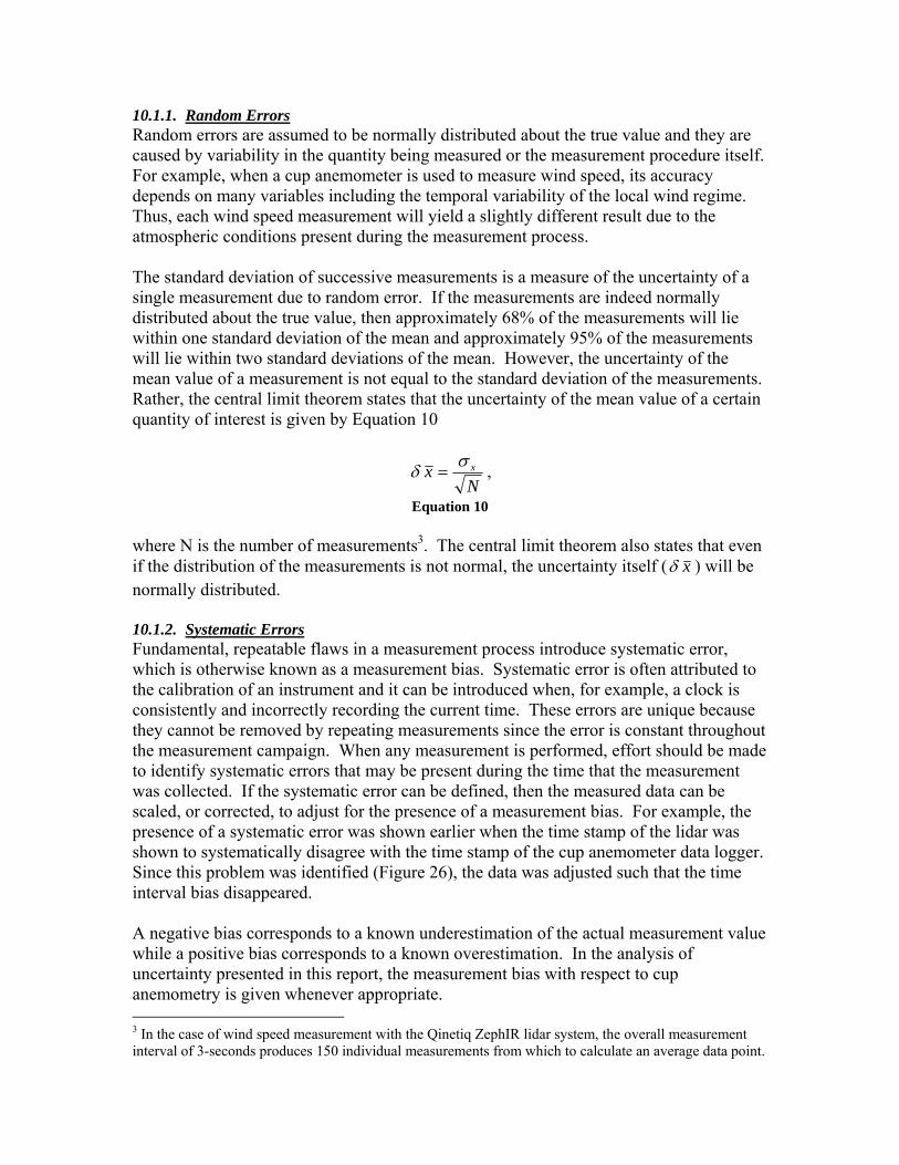
10.1.1. Random Errors Random errors are assumed to be normally distributed about the true value and they are caused by variability in the quantity being measured or the measurement procedure itself. For example, when a cup anemometer is used to measure wind speed, its accuracy depends on many variables including the temporal variability of the local wind regime. Thus, each wind speed measurement will yield a slightly different result due to the atmospheric conditions present during the measurement process. The standard deviation of successive measurements is a measure of the uncertainty of a single measurement due to random error. If the measurements are indeed normally distributed about the true value, then approximately 68% of the measurements will lie within one standard deviation of the mean and approximately 95% of the measurements will lie within two standard deviations of the mean. However, the uncertainty of the mean value of a measurement is not equal to the standard deviation of the measurements. Rather, the central limit theorem states that the uncertainty of the mean value of a certain quantity of interest is given by Equation 10

Nx xσδ = ,

Equation 10 where N is the number of measurements3. The central limit theorem also states that even if the distribution of the measurements is not normal, the uncertainty itself ( xδ ) will be normally distributed. 10.1.2. Systematic Errors Fundamental, repeatable flaws in a measurement process introduce systematic error, which is otherwise known as a measurement bias. Systematic error is often attributed to the calibration of an instrument and it can be introduced when, for example, a clock is consistently and incorrectly recording the current time. These errors are unique because they cannot be removed by repeating measurements since the error is constant throughout the measurement campaign. When any measurement is performed, effort should be made to identify systematic errors that may be present during the time that the measurement was collected. If the systematic error can be defined, then the measured data can be scaled, or corrected, to adjust for the presence of a measurement bias. For example, the presence of a systematic error was shown earlier when the time stamp of the lidar was shown to systematically disagree with the time stamp of the cup anemometer data logger. Since this problem was identified (Figure 26), the data was adjusted such that the time interval bias disappeared. A negative bias corresponds to a known underestimation of the actual measurement value while a positive bias corresponds to a known overestimation. In the analysis of uncertainty presented in this report, the measurement bias with respect to cup anemometry is given whenever appropriate. 3 In the case of wind speed measurement with the Qinetiq ZephIR lidar system, the overall measurement interval of 3-seconds produces 150 individual measurements from which to calculate an average data point.

As discussed earlier, the lidar is known to transmit electromagnetic radiation at a stable wavelength [25]. This means that the frequency drift of the lidar transmitter is negligible. Thus, the systematic errors in the lidar measurement process are assumed here to be insignificant. This assumption is in agreement with a similar lidar uncertainty study performed by Drobinski et al. [36]. This characteristic, however, does not equate to negligible overall measurement error on behalf of the lidar. The sources of uncertainty that pertain to lidar operation are supplied in section 10.3.

10.2. Anemometer Uncertainty: Overview Lackner et al. provides a comprehensive investigation into the sources of uncertainty that influence cup anemometer wind speed measurements in [3]. The sources of error that can be addressed by substituting lidar technology for wind resource assessment are grouped under the category of measurement uncertainty and are defined as:

1. Sensor calibration uncertainty 2. Anemometer dynamic overspeeding 3. Vertical flow effects 4. Vertical turbulence 5. Tower shadow effects 6. Sensor boom effects 7. Data reduction accuracy

In addition to these sources of measurement uncertainty, Lackner defines another category, site assessment uncertainty. Included in this grouping is:

8. Wind shear model uncertainty There are, however, many more sources of uncertainty in wind resource monitoring that are not listed above. This report will focus on the eight sources of uncertainty that are relevant to the use of laser remote sensing in place of cup anemometers for wind speed measurement. Each respective source of cup anemometer uncertainty, CXUδ , can be quantified and summed using a root-sum-square method to define its contribution to the overall uncertainty of a wind resource assessment that employs the use of cup anemometers for measurement. Further detail about the root-sum-square method is given in section 10.3. The uncertainties can be combined using this approach because they are assumed to be independent of one another. Descriptions of these eight components of cup anemometer uncertainty are individually summarized below. The above sources of error are then summed to yield an approximation of the overall measurement uncertainty that is associated with cup anemometer wind speed measurement.

10.2.1. Anemometer Uncertainty: Sensor Calibration Uncertainty The process by which an anemometer of a particular design is calibrated is itself subject to measurement error. This introduces uncertainty that is associated with the sensor calibration process. Furthermore, since each production anemometer is slightly different from the test model, the presence of additional measurement uncertainty is possible. According to the work done by Lockhart and Bailey, the role of anemometer calibration uncertainty contributes approximately 0.1-2% uncertainty when the NRG Maximum 40 anemometer is used [37]. As a general rule, Lackner estimates that sensor calibration uncertainty should be conservatively approximated as %5.11 =CUδ . 10.2.2. Anemometer Uncertainty: Anemometer Dynamic Overspeeding Anemometer overspeeding is a well-known source of wind speed measurement error that is caused by the presence of longitudinal, or horizontal, turbulence. The basic design of a cup anemometer causes it to speed up more rapidly than it slows down. In the event of turbulent wind flow, this inherent design trait introduces a positive bias that causes an overestimation of the true wind speed. It follows that anemometer overspeeding is a function of turbulence intensity (defined in Equation 9) [38]. A study performed by Kristensen concluded that the error associated with longitudinal overspeeding is proportional to the square of the horizontal turbulence intensity. Furthermore, this study states that the dynamic response of a cup anemometer should be characterized by a unique distance constant rather than its time constant [39]. While this source of error is dependent on the local wind regime, Lackner contends that uncertainty associated with longitudinal anemometer overspeeding should be approximated as %3.02 =CUδ , which introduces a 0.5% positive measurement bias [3]. 10.2.3. Anemometer Uncertainty: Vertical Flow Effects The IEC requires that the horizontal (lateral or longitudinal) component of the wind speed is used when the power curve of a wind turbine is calculated [34]. Thus, the goal of wind resource assessment is to record the horizontal wind speed so that power production estimates will correspond closely to the power curve of a candidate wind turbine. Certain anemometer models measure the horizontal, or two-dimensional, wind components better than others, but all cup anemometers capture some part of the vertical wind vector, which in turn introduces measurement error to the wind data. The capacity of an anemometer to measure the horizontal component of the wind speed is described by its angular, or tilt, response to wind that approaches from the vertical direction. The angular response of the NRG Maximum 40 anemometer is shown below in Figure 50. If the sensor were an ideal three-dimensional anemometer, the response to flow inclination would be a flat line, indicating that the anemometer would measure the true 3D wind speed at any tilt angle. While the Maximum 40 anemometer is capable of measuring the full 3D wind speed at a wide variety of tilt angles, the erratic behavior of the response curve suggests that it is subject to significant vertical flow effects.

Figure 50: NRG Maximum 40 Tilt Response [40]

Lackner defines the measurement uncertainty contribution of vertical flow effects in flat terrain as %5.03 =CUδ . 10.2.4. Anemometer Uncertainty: Vertical Turbulence Effects Just as dynamic overspeeding introduces uncertainty that is caused by the presence of horizontal turbulence, vertical turbulence effects are introduced by the presence of vertical turbulence in the wind. Turbulence intensity is found according to Equation 9. This parameter can be decomposed into Cartesian coordinates where the lateral, longitudinal and vertical components of turbulence intensity can be found. The longitudinal direction is horizontal and in the direction of the mean wind speed. The lateral direction is perpendicular to the vertical and longitudinal directions. Thus, each component of turbulence intensity is equal to the standard deviation of the wind speed component in the respective directions, divided by the overall mean wind speed. Lackner maintains that a conservative estimate for the uncertainty that is associated with vertical turbulence is %24 =CUδ when the NRG Maximum 40 anemometer is used in flat terrain. This source of uncertainty introduces a positive measurement bias of 3% in flat terrain. 10.2.5. Anemometer Uncertainty: Tower Shadow Effects When anemometers of any type are mounted on a tower, the tower structure itself introduces an obstruction that inhibits the free-stream flow of air to the sensor. The error that is associated with the obstruction of airflow is grouped in two categories: tower shadow effects and sensor boom effects. The wind speed measurement uncertainty associated with sensor boom effects is discussed in the following section.

As a standard rule of thumb, locating the anemometer a distance of approximately 6 tower diameters away from a tubular tower structure can drastically minimize tower shadow effects. However, in the case of lattice tower structures, it becomes much more difficult to avoid significant tower shadow effects. Lackner suggests that the uncertainty associated with measurements made using single-side-mounted anemometers is 1%. Since each set of two cup anemometers at the WBZ tower were mounted on one side of the tower, the uncertainty associated with tower shadow effects is %0.15 =CUδ . This uncertainty introduces a -1.5% overall measurement bias [3]. 10.2.6. Anemometer Uncertainty: Sensor Boom and Mounting Effects The booms on which tower-mounted cup anemometers are positioned also disturb the free-stream flow of air to the sensors. Furthermore, when an anemometer is not positioned vertically, measurement error is introduced. The uncertainties associated with these sources of error are grouped in the sensor boom and mounting effects category. The overall uncertainty contribution of these factors can be estimated as %5.06 =CUδ [3]. 10.2.7. Anemometer Uncertainty: Data Reduction Accuracy The final source of cup anemometer measurement uncertainty is associated with the amount of data that are removed in the process of filtering the wind speed data after it has been collected. Wind data are traditionally groomed to eliminate instances where, for example, the sensors were partially or completely enshrouded by ice. Another common problem is sensor failure. When data are removed during these instances, the erroneous records are replaced by gaps that do not contribute to wind speed estimates. Thus, an uncertainty in the wind monitoring process develops that is a function of the length and distribution of the gaps that are caused by missing data. After removing increasingly large amounts of data from random points in the time series data set, Lackner found that the uncertainty associated with missing data can be approximated as )missing(%*03.0=Uδ . In a one-year wind resource measurement campaign it is reasonable to assume that approximately 5% of the wind data could be lost due to some operational problem(s) when cup anemometers are used. When 5% of the data are missing, the uncertainty associated with data loss becomes %2.07 =CUδ . 10.2.8. Anemometer Uncertainty: Wind Shear Model Uncertainty Wind turbine energy production estimates are most accurate when wind speed data at the hub height of a modern wind turbine are available. However, a variety of constraints prohibit actual measurements from being obtained at such heights. Since the wind speed in the atmospheric boundary layer typically increases with height, a wind shear model is therefore used to extrapolate the estimated wind speed data to the hub height of a wind turbine. This extrapolation can be done using the log law, shown below in Equation 11, where z and zr are the target and reference heights, U(z) and U(zr) are the target and reference height wind speeds and zo is the surface roughness length.

U(z)U(zr )

=ln z

z0

⎛

⎝ ⎜

⎞

⎠ ⎟

ln zr

z0

⎛

⎝ ⎜

⎞

⎠ ⎟

Equation 11 Another common wind shear model is the power law where the equation variables are defined above and alpha is the power law exponent.

U(z)U(zr)

=zzr

⎛

⎝ ⎜

⎞

⎠ ⎟

α

Equation 12 A study performed by Elkinton et al. concluded that both models yield similar results for wind speed extrapolation. Furthermore, this study showed that the use of either wind shear model has no direct benefit over the other and that both models may or may not yield erroneous wind speed estimates upon extrapolation to hub height [41]. Thus, wind shear extrapolation is a significant source of wind resource assessment uncertainty and often the largest. The results summarized by Elkinton and Lackner suggest that the uncertainty associated with shear extrapolation on flat terrain can be estimated as

%0.68 =CUδ [41],[3]. This uncertainty does not apply to the specific case of the wind resource assessment study at the Hull WBZ site because wind speeds were measured well above 80 meters (the approximate hub height of a modern wind turbine). However, for the purpose of illustrating the generic sources of uncertainty associated with traditional meteorological tower wind resource monitoring, this component will be included in the overall uncertainty analysis. 10.2.9. Anemometer Uncertainty: Summary Table 16 shows the summary of uncertainty sources that are associated with cup anemometer wind speed measurement. The first seven entries in Table 16 are classified in the “measurement uncertainty” grouping. The last entry in Table 16, 8CUδ , falls under the category of “site assessment uncertainty.” It is included in this uncertainty analysis to illustrate the advantage that remote sensing offers with respect to eliminating the need for wind speed extrapolation.

Uncertainty Source Component Uncertainty

Calibration Uncertainty ( 1CUδ ) 1.5% Dynamic Overspeeding ( 2CUδ ) 0.3% Vertical Flow Effects ( 3CUδ ) 0.5% Vertical Turbulence Effects ( 4CUδ ) 2.0% Tower Shadow Effects ( 5CUδ ) 1.0% Sensor Boom and Mounting Effects ( 6CUδ ) 0.5% Data Reduction Accuracy ( 7CUδ ) 0.2% Wind Shear Model Uncertainty ( 8CUδ ) 6.0%

Table 16: Cup Anemometer Uncertainty Summary

10.3. Lidar Uncertainty: Overview

The lidar’s main appeal is its ability to collect wind speed data at the hub height of a modern wind turbine while remaining portable, accurate and silent. However, as shown in previous sections, the lidar is indeed subject to some degree of measurement error that can be associated with a number of factors, such as:

1. Error in the estimation of the return Doppler spectrum 2. Uncertainty of the mean Doppler frequency shift estimation 3. Frequency drift in the local oscillator beam 4. Wind turbulence in the lidar probe volume 5. Error in the non-linear least squares data fit 6. Weak atmospheric backscatter 7. Measurement range uncertainty 8. Improper instrument setup 9. Data reduction accuracy

This section will quantify the sources of measurement error that are associated with the above random sources of uncertainty. Throughout this analysis, the various sources of error will be presented in nondimensionalized format. Each respective source of uncertainty, LXUδ , can be quantified and summed using a root-sum-square method to define its contribution to the overall uncertainty of a wind resource assessment that employs the use of a lidar for wind speed measurement. Further detail about the root-sum-square method is given in section 10.3. The uncertainties can be combined using this approach because they are assumed to be independent of one another. 10.3.1. Lidar Uncertainty: Error in Doppler Spectrum Estimation For optimum sensitivity, the noise level of a CLR system must be dominated by spectrally flat shot noise originating from the local oscillator [15]. However, it is

conceivable that stray light of another frequency and wavelength may corrupt the lidar aerosol backscatter signal. This event introduces excess noise in the photodetector signal, which results in a Doppler wind spectrum that does not represent the actual frequency content of the wind field that is being probed. The level of signal interference depends on the intensity of stray light, the laser coherence time, τ c , the delay time between the stray light and the local oscillator, τd , detector responsivity ℜ and the effective frequency detection bandwidth B. The excess noise in the photodetector signal current can be estimated by Equation 13 where PT and PS are the respective powers of the laser beam during transmission and upon detection [15].

iExcess2 ≅ ℜ2 2PT PS

πτ d

2

τ c

B

Equation 13 The excess noise in the photodetector signal current is time-averaged (indicated by the angle brackets) over the amount of time required to estimate a single Doppler spectrum. A single Doppler spectrum is calculated in ~5µs for the Qinetiq ZephIR lidar [14]. It is possible to reduce the major contributions of excess noise in the Doppler spectrum estimation process by averaging over several spectral measurements. The ZephIR calculates and averages 4,000 spectra for each wind speed estimation. This calculation process requires a total of roughly 20 ms of time. This is called the integration time. In order to further understand the importance of spectral averaging, the signal-to-noise ratio (SNR), shown in Equation 14, must be considered for a CW CLR system.

SNR =ηPS

hcλ

⎛ ⎝ ⎜

⎞ ⎠ ⎟ B 1+ D + R( )

Equation 14 Here η is an efficiency term incorporating optical losses and photodetector sensitivity,

is the input signal power derived from Equation 2. The term

SP

⎟⎠⎞

⎜⎝⎛

λhc is the light quantum

energy of order J and B is the signal bandwidth. The remaining terms, D and R, represent the power spectral density from dark noise and RIN respectively (excess noise). A study performed by Karlsson et al. shows that D and R in the SNR expression above can be related to Equation 13 by observing the fluctuations of the relative phase between the local oscillator and the stray light that causes excess noise to interfere with the return signal [15].

191028.1 −×

The SNR is the power spectral density at the Doppler peak divided by that of the surrounding noise floor. By averaging multiple wind spectra, the excess noise is reduced which thereby increases the SNR. When the SNR is maximized, the most accurate wind

velocity measurements are possible. Thus, the wind spectra averaging process is indeed crucial to the accuracy of the wind velocity data that the ZephIR reports. It can be shown that the error in the Doppler spectrum estimation is governed by Equation 15 [28].

( ) Am

As11 +−=ε

Equation 15 The error in the Doppler spectrum estimation, sε , is a function of m, the number of single spectra measured during the integral time and A, a complex term that describes the spatial resolution of the lidar beam. Further detail on A is given in [28]. When the lidar probe volume becomes large, A tends to unity. Therefore, when the lidar measures at longer range (e.g. heights in excess of 80-100 meters), the error in the Doppler spectrum estimation reduces with the square root of m. Each 3-second lidar measurement average is a result of averaging up to 150 line-of-sight data points in the non-linear curve-fitting algorithm. As described earlier, this number of data points is only possible when the atmospheric backscatter coefficient is maximized. It can be shown that the average number of line-of-sight wind speed data points is approximately 105 in realistic conditions. Each of the 105 line-of-sight data points are obtained by averaging 4,000 total spectra. The relative error associated with each

spectral measurement is 4000

1 , or approximately 1.6%. This error is then averaged

105 times for each 3-second measurement average. The resulting uncertainty in the Doppler spectrum estimation process is conservatively approximated as %2.01 =Lδ . 10.3.2. Lidar Uncertainty: Error in Mean Doppler Frequency Shift As described earlier, the ZephIR analyzes averaged wind spectra and obtains the mean Doppler shifted frequency by applying an algorithm that calculates the first moment (center of gravity) of the spectra around the frequency peak. This is in agreement with the method used by Karlsson et al. for wind measurements in the atmospheric surface layer [15]. When the mean frequency is determined, it is substituted in Equation 16 to estimate the line-of-sight wind velocity.

f Shifted =2λ

vLOS

Equation 16 Error is introduced when the mean Doppler frequency shift is incorrectly estimated in this process.

The general expression for variance of Equation 16 can be shown to include two terms. The first term represents the variance of the line-of-sight component of the wind velocity

measurement averaged over the probe volume. The second term describes the received detector signal fluctuations (averaged over the integration time) that are caused by random variations of scattering particles relative to each other due to turbulence. In practice, Equation 17 is used to simplify the estimate of the variance of the mean Doppler frequency shift estimation [28].

σ f2 = 0.26 σ LOS

2 λ

t0(∆zεT )1

3,

Equation 17 Equation 17 includes σ LOS

2 , the variance of the line-of-sight velocity measurements, t0, the integration time (20ms), λ, the laser wavelength, and εT , the rate of turbulent energy dissipation. At a height of 100 meters, the lidar probe depth (∆z ) is 17.9 m. Assuming a turbulent energy dissipation rate of 10-2 m2/s3 and line-of-sight velocity standard deviation of 3 m/s, the standard deviation of the mean Doppler frequency shift is 0.018 m/s. Since the lidar is typically used to measure wind speed and direction at heights between 40 meters and 120 meters, the average uncertainty associated with this source of error is estimated with Equation 10 to be %2.02 =Lδ . 10.3.3. Lidar Uncertainty: Frequency Drift in the Local Oscillator Beam An earlier study lead by Jorgensen concluded that the frequency drift of the ZephIR beam upon transmission suffers negligible divergence (less than 0.2%) over extended periods of time [26]. As shown in Figure 4, the lidar beam is referenced by the local oscillator in order to determine the frequency of emitted light. In addition to the work of Jorgensen et al., general pulsed lidar systems are also shown to exhibit insignificant frequency drift in [44] and [45]. As such, the uncertainty associated with frequency in the local oscillator beam is assumed in this analysis to be negligible; %0.03 ≅Lδ . 10.3.4. Lidar Uncertainty: Non-uniform Airflow in the Lidar Probe Volume In a study performed by Frehlich, the effects of turbulence on the accuracy of pulsed coherent Doppler lidar were considered [42]. In this study, various approximations for the mean line-of-sight wind speed velocity are considered using both computer simulated data and actual data from a 2µm pulsed Doppler lidar. This study used the Kolmogorov spectrum outer scale of turbulence to model the characteristics of a turbulent wind field4. The study concludes that the measurement error associated with non-uniform airflow in the lidar probe volume is caused by random variations of the radial wind velocity component (vLOS) and the random location of the aerosol particles in relation to one another. These phenomena combine to produce a lidar return signal with random attributes that can affect the overall wind speed measurement accuracy. Frehlich finds that the actual, ensemble-averaged lidar wind speed estimations are subject to between 0.5% and 20% error for realistic conditions. This range of error is shown to be a function

4 Outer scale turbulence is caused by large air mass flow and the Kolmogorov spectrum gives the distribution of energy among turbulence vortices as function of vortex size

of ∆pL0

, the ratio of the Doppler pulse width ∆p (analogous to the probe depth ∆z for CW

Doppler lidar) to the turbulence outer scale, . In practice, the lidar probe depth is generally much smaller than the turbulence outer scale and depending on the measurement range the CW lidar probe depth is approximately 4-9% of the turbulence

outer scale [28]. Furthermore, when the ratio

L0

1.00

<∆L

p , the velocity estimation error

associated with turbulent airflow in the lidar probe volume is well defined [42]. The average error associated with non-uniform airflow in the lidar probe volume is estimated to be 4-5%, which is in agreement with the findings of Frehlich. Thus, the uncertainty associated with turbulent airflow in the lidar probe volume is estimated to be %0.54 =Lδ . 10.3.5. Lidar Uncertainty: Error in the Non-Linear Least Squares Data Fit Section 5.5 describes the operation of the curve fitting algorithm that performs a non-linear least squares fit on the lidar line-of-sight wind velocity data. This fitting algorithm is implemented for the purpose of obtaining the horizontal and vertical wind speed from the coefficients in Equation 4. This curve-fitting algorithm is a form of regression analysis. An unavoidable characteristic of regression analyses is that when any curve fitting operation is executed, error in the estimated best-fit parameters is introduced. This section describes a method by which the uncertainty in the wind speed parameter extraction process is obtained for applications where the ZephIR lidar is used. Ideally, actual line-of-sight lidar data would be used to quantify the mean variance of the best-fit curve. Unfortunately the ZephIR manufacturer does not grant access to these data. Therefore, another approach must be considered. An alternative method for studying the uncertainty associated with the curve-fitting algorithm is to generate simulated data and implement a non-linear least squares fit on these data. When the wind speed parameters are extracted in this manner, the variance about the best-fit curve can be calculated. This approach allows this individual component of lidar measurement uncertainty to be isolated and explicitly defined. Figure 51 shows the behavior of the line-of-sight wind data that are measured by the lidar. Here, 105 data points are produced with a random number generator for the simulation of actual lidar data. Recall that the lidar obtains an average of 105 line-of-sight wind speed measurements in each 3-second measurement period.

Figure 51: Line-of-Sight Wind Velocity vs. Lidar Azimuth Scan Angle

Figure 52 illustrates the behavior of the line-of-sight wind data with greater detail. These data are generated under relatively turbulent conditions to obtain a more realistic representation of the wind speed measurement uncertainty associated with the curve-fitting algorithm. The peaks in Figure 52 occur at the maximum up-wind and down-wind speeds over each rotation of the lidar beam.

Figure 52: Detail of Line-of-Sight Wind Velocity vs. Lidar Azimuth Scan Angle

The estimation of horizontal wind speed measurement uncertainty is completed with more than five hundred curve-fit iterations in a computer program. The resulting uncertainty associated with the wind speed parameter extraction process is %1.05 ≅Lδ . This value pertains to the uncertainty in a typical 10-minute wind speed average. 10.3.6. Lidar Uncertainty: Aerosol Backscatter Coefficient Under conditions of high atmospheric backscatter, the lidar return signal power (defined in Equation 2) is maximized and more accurate wind spectra are produced. This corresponds to a circumstance where more exact line-of-sight wind speed measurements are possible. This is possible because the signal-to-noise ratio is much larger than unity and thus, the average frequency of the backscattered light is well defined. As the atmospheric backscatter coefficient decreases (associated with increased air clarity), accurate wind speed measurements become more difficult. This is associated with return signal attenuation where the SNR can drop to unacceptable levels. A study performed by Liu, et al. concludes that the uncertainty of Doppler line-of-sight wind velocity measurements is less than 0.2 m/s when the ratio of aerosol ( aβ ) to molecular ( mβ ) volume backscatter coefficients is in the range of 6-19 [43]. This range of the ratio of aerosol to molecular volume backscatter coefficients is common in the lower atmospheric boundary layer. Typically, the aerosol backscatter coefficient ratio increases dramatically as measurement range decreases as shown in Figure 53.

Figure 53: Example of Atmospheric Backscatter Ratio as a Function of Measurement Range [43]

To protect against the possibility of recording erroneous wind speed measurements, the ZephIR records a -9999 error message if extremely clear conditions are present. When such conditions do occur (typically on cold and extremely clear days), the number of valid line-of-sight data points in the non-linear least squares fit drops below a certain threshold. When this occurs, the lidar instrument disqualifies the measurements. Thus, the measurement uncertainty associated with weak aerosol backscatter is assumed to be negligible for the ZephIR lidar instrument. This is associated with the fact that large levels of atmospheric backscatter are characteristically present at heights below 150

meters as well as the proven efficacy of the lidar low backscatter safeguard. Therefore, %0.06 ≅Lδ .

10.3.7. Lidar Uncertainty: Range Accuracy Continuous wave Doppler lidar systems are susceptible to wind speed measurement error associated with uncertainty in the measurement range. This error is unavoidable because the height at which the lidar probes the atmosphere is determined by the adjustment of internal optics that are not always accurate. As such, the lidar may not actually probe the user-programmed measurement height, but rather some other height as governed by the variability of the measurement range. The range accuracy, defined as one standard deviation, is given by Equation 18 [15].

mod4 ffc f

R ∆=

σσ

Equation 18 The range accuracy is a function of c, the speed of light and fσ the standard deviation of the frequency measurement. The terms f∆ and are modulation parameters that vary widely from system to system. The exact modulation parameters for the ZephIR system are not known, but they are assumed here to be 1 kHz and 1.3 GHz respectively. These values agree with a similar system performed in a test by Karlsson et al. [15]. This study finds that the range accuracy for a 1.55µm continuous wave coherent laser radar system is approximately 6 meters when the signal-to-noise ratio is low. In a wind regime with moderately strong wind shear characteristics (α = 0.20), the associated measurement error at 100

modf

+6 meters is 0.09 m/s in an 8 m/s average wind regime. As such, the overall wind speed measurement uncertainty associated with lidar range accuracy is %2.17 =Lδ . 10.3.8. Lidar Uncertainty: Improper Instrument Setup When the lidar system is deployed in the field, it must be installed such that the instrument is level. If the instrument is not leveled properly by the operator, it will cause the system to probe a volume of air that is not horizontal. This circumstance causes a particular sector of the lidar scan azimuth to probe winds at a higher height than other portions of the same scan. In areas where the wind shear is strong, this may introduce an overestimation of the actual wind speed at a given height. However, the threat of severe installation mistakes is relatively low since the position of the instrument is always fine-tuned with a sensitive level. Small tilt angles can, however, cause measurement error in realistic applications. When the lidar measures at a range of 100 meters, each degree of tilt at the instrument corresponds to 2.02 meters of overall altitude divergence between opposing sides of the conical scan area. This uncertainty corresponds to a measurement uncertainty of approximately 0.03 m/s in an 8 m/s average wind regime with moderately strong wind shear characteristics (α = 0.20). Thus, a conservative estimation for the uncertainty associated with improper instrument setup is %4.08 =Lδ .

10.3.9. Lidar Uncertainty: Data Loss Another source of measurement uncertainty is associated with the amount of data that are lost during the course of the measurement campaign. The ZephIR lidar is designed to operate in a variety of severe weather conditions. However, it is unlikely that it is consistently capable of robust operation when compared to, e.g., cup anemometer data loggers. The lidar’s reliability problems are demonstrated in the lidar data validation experiment where normal operation was interrupted on several occasions. The threat of future interruptions has since been minimized by outfitting the lidar system with another level of power backup capacity. The fact remains that the reliability of the lidar has not been repeatedly demonstrated in resource assessment applications. When data are lost during operational interruptions, the missing records are replaced by gaps that do not contribute to wind speed estimates. Thus, an uncertainty in the wind monitoring process develops that is a function of the length and distribution of the gaps that are caused by missing data. By removing increasing amounts of data from random points in wind data sets, the uncertainty associated with missing data can be approximated as )missing(%*03.0=Uδ [3]. In a one-year wind resource measurement campaign it is reasonable to assume that approximately 10% of the wind data could be lost due to some operational problem(s) when lidar technology is used. When 10% of the data are missing, the uncertainty associated with data loss becomes %3.09 =Lδ . 10.3.10. Lidar Uncertainty: Summary The overall sources of uncertainty for laser-based wind speed measurement with the ZephIR lidar are summarized in Table 17.

Uncertainty Source Component Uncertainty

Error in the estimation of the return Doppler spectrum ( 1LUδ ) 0.2%

Uncertainty of the mean Doppler frequency shift estimation ( 2LUδ ) 0.2%

Laser Frequency Drift ( 3LUδ ) 0.0%

Wind turbulence in the lidar probe volume ( 4LUδ ) 5.0%

Error in the non-linear least squares data fit ( 5LUδ ) 0.1%

Weak atmospheric backscatter ( 6LUδ ) 0.0%

Measurement range uncertainty ( 7LUδ ) 1.2%

Improper instrument setup ( 8LUδ ) 0.4%

Data loss ( 9LUδ ) 0.3%

Table 17: Lidar Uncertainty Summary

The sources of measurement uncertainty that are presented in Table 17 are combined in a combined value for overall uncertainty in section 10.3.

10.4. Lidar and Cup Anemometer Overall Uncertainty Comparison In this section, the various sources of uncertainty for each sensor are summed to yield an overall quantity for uncertainty in wind speed measurement. These values are calculated using a root-sum-square method for determining the overall uncertainty of a value that is a function of several variables. When the wind speed U is a function of several variables,

, the uncertainties of the variables, ),...,( 1 nxxfU = nxx δδ ,...,1 , can be combined to yield an overall uncertainty using Equation 19 [35].

22

11

... ⎟⎟⎠

⎞⎜⎜⎝

⎛∂∂

++⎟⎟⎠

⎞⎜⎜⎝

⎛∂∂

= nn

xxUx

xUU δδδ

Equation 19 Equation 19 can be non-dimensionalized so that the uncertainties of the variables are expressed as fractions. The non-dimensional form of Equation 19 is shown in Equation 20. Here, the partial derivatives and the fractions, which multiply the fractional uncertainties, are referred to as “sensitivity factors.” Sensitivity factors measure the responsivity of changes in wind speed measurements (U) to the individual variables ( ). If the wind speed measurement has a linear dependence on a variable, then the sensitivity factor will be one for that variable. For a quadratic dependence, the sensitivity factor will be two. These sensitivity factors are also non-dimensional. Notice that if U depends linearly on all of the variables in Equation 20, then the expression becomes a simple root-sum-square relationship.

nxx ,...,1

22

11

1

... ⎟⎟⎠

⎞⎜⎜⎝

⎛∂∂

++⎟⎟⎠

⎞⎜⎜⎝

⎛∂∂

= nn

n

xf

xxUx

fx

xUU δδδ

Equation 20 The uncertainty associated with lidar wind speed measurement is now presented. The component sources of lidar measurement uncertainty are summarized in Table 17. The equation for the lidar wind speed measurement uncertainty is given in Equation 21. Each of the seven components of uncertainty in Equation 21 corresponds to a separate source of measurement uncertainty that is defined in previous sections above.

( ) ( ) ( ) ( ) ( ) ( ) ( ) ( ) ( )28

28

27

26

25

24

23

22

21LIDAR LLLLLLLLL UUUUUUUUUU δδδδδδδδδδ ++++++++=

Equation 21

Using Equation 20, the non-dimensionalized overall lidar measurement uncertainty is given in Equation 22 where the sensitivity factor, , is equal to one. is unity because the measurement of the horizontal wind speed depends linearly on all of the variables in Equation 21.

LIDARSF LIDARSF

δULIDAR _ Overall = SFLIDAR ⋅ δULIDAR( ) Equation 22

The overall lidar measurement uncertainty is %2.5_ =OverallLIDARUδ . The uncertainty associated with cup anemometer wind speed measurement is now presented. The component sources of cup anemometer measurement uncertainty are summarized in Table 16. The equation that defines the overall cup anemometer uncertainty combines eight sources of uncertainty. Seven of these sources of uncertainty are associated with measurement error ( 1CUδ through δUC 7) and one source of uncertainty associated with wind shear extrapolation uncertainty (δUC 8). When these uncertainty components are grouped together, they have subscripts “measurement” and “shear model” respectively. Cup anemometer measurement uncertainty is defined in Equation 23. Each of the seven components of uncertainty in Equation 23 corresponds to a separate source of measurement uncertainty that is defined in previous sections above. δUCups _ Measurement = δUC1( )2 + δUC 2( )2 + δUC 3( )2 + δUC 4( )2 + δUC 5( )2 + δUC 6( )2 + δUC 7( )2

Equation 23 The sensitivity factor for cup anemometer measurement uncertainty, , can be written as an analytic function of three measurement heights as shown in Equation 24 [3]. The measurement heights h

SFCups _ Measurement

1, h2 and h3, in this case, correspond to the three measurement heights on the WBZ radio tower: 118 m, 87 m and 61 m respectively.

SFCups_ Measurement =

2 ln h3

h2

⎛

⎝ ⎜

⎞

⎠ ⎟

⎛

⎝ ⎜

⎞

⎠ ⎟

2

+ ln h2

h1

⎛

⎝ ⎜

⎞

⎠ ⎟

⎛

⎝ ⎜

⎞

⎠ ⎟

2

+ 2ln h2

h1

⎛

⎝ ⎜

⎞

⎠ ⎟ ln

h3

h2

⎛

⎝ ⎜

⎞

⎠ ⎟

ln h2

h1

⎛

⎝ ⎜

⎞

⎠ ⎟

⎛

⎝ ⎜

⎞

⎠ ⎟

2

Equation 24 The shear model measurement uncertainty, δUShear Model , is defined above and is equivalent to 8CUδ . The sensitivity factor for the shear model uncertainty is one [3]. These relationships and the expressions in Equation 23 and Equation 24 are combined to form the equation for the overall cup anemometer uncertainty. This expression is presented in Equation 25.

δUCup _ Anemometer_ Overall = SFCups_ Measurement ⋅ δUCups_ Measurement( )2+ SFShear Model ⋅ δUShear Model( )2

Equation 25

The total cup anemometer uncertainty is δUCup _ Anemometer _ Overall = 8.3%.

10.5. Uncertainty Analysis Summary of Results The overall measurement uncertainty for the lidar and the cup anemometers is presented in Table 18. Here, the lidar is generically shown to minimize the wind speed measurement uncertainty when compared to applications where the NRG Maximum 40 is used.

Uncertainty Source Wind Speed

Measurement Uncertainty

Overall Lidar Measurement Uncertainty (δULIDAR _ Overall ) 5.2% Overall Cup Anemometer Measurement Uncertainty (δUCup _ Anemometer _ Overall ) 8.3%

Table 18: Overall Uncertainty Summary It is important to note that the overall sources of uncertainty summarized in Table 18 pertain to generic cup anemometer and Doppler lidar measurements. The various components of error that contribute to the overall uncertainty are compiled in this manner for the purpose of maintaining uniformity throughout the head-to-head uncertainty comparison. There are several more sources of cup anemometer uncertainty that introduce error in the estimation of the long-term average wind speed. The cup anemometer uncertainty components that are summarized above are limited to the sources that are commensurate with lidar wind speed measurement. A more detailed analysis of long-term cup anemometer measurement uncertainty for wind power applications is given in [3]. 11. Discussion and Lessons Learned

11.1. Validation Experiment Data Summary The data summarized in the lidar validation experiment were collected between December 2nd 2006 and February 13th 2007. This period includes approximately 14 days of missing lidar data, all of which were caused by three separate power interruptions. Rigorous data grooming caused the total length of concurrent data at each height to be different because unique filters were applied at each of the three measurement levels. Table 19 summarizes the amount of concurrent wind speed data that were available for comparison.

Measurement Height [m]

Number of Data Records

After Filtering [ ]

Percent of Total [%]

Total Length of

Concurrent Data [Days]

61 7270 68.7% 50.5 87 6065 57.4% 42.1 118 6771 64.1% 47.0

Table 19: Total Amount of Concurrent Data Used for Comparisons

Fewer data records were available at 87 meters because the sensor boom at this measurement level was blown out of alignment during a period of high wind speeds. Because the wind speed sensors at this level were moved closer to the tower, their response to the tower speed-up and slow-down effects are more dramatic. This causes the various data filters to remove a greater amount of data at the 87 meter sensor level (see also, Figure 23). The result of filtering the cup anemometer wind speed data permitted the use of the WBZ data as an experimental control. The lidar’s performance at each of the three measurement heights demonstrates strong and consistent correlation with the cup anemometers at the same height. The lidar established proof that it is capable of successfully replicating the wind speed measurements that are recorded by tower-mounted cup anemometry at each of the three measurement heights. 11.1.1. Tower Data Throughout the course of the data validation experiment, two main problems emerged relating to the validity of the tower data set. First, the wind direction sensors were not positioned properly when the equipment was initially installed. This issue was corrected by adding a wind direction offset to the data at all three measurement heights. The sensor boom at the 87-meter level was later blown out of alignment with respect to the other two sensor booms so extra care was taken to confirm that the data at this height were valid. The second problem with the cup anemometer data relates to instances where temporary periods of measurement disagreements were observed. These measurement disagreements were determined to occur only during certain wind speed events and their erroneous nature was confirmed by comparison with wind speed data from another nearby meteorological tower. Both of these problems were identified, addressed and successfully resolved such that the WBZ wind speed data have achieved the level of quality that is expected of an experimental control. 11.1.2. Lidar Operation 11.1.2.1. Power Interruption During the measurement campaign, the lidar lost power on three separate occasions. The most severe instance occurred during the first week of the experiment and was caused by a failure of the battery charging controller. Upon further investigation the battery pod printed circuit board (PCB) was found to be in disrepair. The failure of the PCB also caused the backup batteries to discharge completely because the controller failed to protect the batteries from being drained past their recommended minimum voltage level. The actual explanation for the cause of this malfunction remains unknown. Power was later restored to the system when the manufacturer sent a replacement PCB. Two temporary lead-acid batteries were substituted for the four gel cell batteries that came with the lidar.

The system operated flawlessly throughout the month of December but later encountered another operational failure when the external power supply was temporarily interrupted. As shown in Figure 54, this short interruption caused the lidar to shut down immediately. The behavior of the lidar battery voltage signal exhibited no irregularities before the power disruption occurred, indicating that the lidar did not implement its battery backup safeguard. If the battery backup system were functioning properly, it is expected that the voltage level would decrease before the instrument would shutdown on the basis of low power.

Power Interruption

Figure 54: Lidar Battery Voltage Time Series Just before a Power Interruption It was later determined that the temporary battery backup system (2 lead acid battery substitutes in place of the original 4 gel cell batteries) were not capable of serving as power surge protectors. The battery backup system was not functioning properly during the experimental campaign and as a result, any interruption in the external power supply resulted in a full system shutdown. Each such instance required a manual restart of the system before it was possible to collect data once again. In order to prevent the future recurrence of this phenomenon, an external battery bank and four new gel cell batteries will be included before the lidar is dispatched on its next assignment. Also, the threat of power loss underscores the importance of a reliable and accessible site contact representative who can physically inspect the lidar if power and communication are lost again in the future. 11.1.2.2. Operating Temperature Another source of concern for the reliable operation of the lidar is the temperature at which the instrument operates. The lidar incorporates electric heaters in the three system pods that regulate the internal temperature during cool weather. During normal operation, the internal temperature of the lidar is held above approximately 20ºC because

the most accurate background noise floor is determined when a stable and warm operating temperature is achieved. If the operation of the lidar is interrupted during periods where the external temperature is less than 5ºC, then the instrument must reheat itself to above 20ºC before it can make an accurate estimate of the background noise intensity level. This fact, while tremendously significant to the short-term validity of the data upon cold startup, is not reported in the user’s manual. If left unchecked, the lidar data measurements can overestimate the cup anemometer wind speeds by more than 10 m/s before a reasonable estimation of background noise is acquired. In the case of the data validation experiment, this circumstance was observed each of the three times that the lidar was manually restarted after a power interruption. The solution to this potential source of measurement discrepancy is a simple removal of the first three hours of data when the system is started during periods of cold ambient temperatures. During the data validation experiment, this solution was applied after each of the three instances of power failure. Thus, the wind speed data do not exhibit any irregularities associated with a flawed estimation of the noise floor. 11.1.2.3. Flash Card Data Retrieval Under normal circumstances the lidar data can be downloaded efficiently via an Ethernet or GSM modem connection for any user-defined averaging period (600 seconds is typical). However, there are certain unknown conditions that cause the data index file to become corrupted. When the index becomes corrupted, any attempt to remotely download new data is met with an error message. The only alternative for data retrieval in this instance is to physically remove the compact flash data card and manually download the data. When the data are retrieved by this process the only form that they can take are 3-second averaged records. This requires the user to separately convert the 3-second average data to any other averaging period that they may require. Furthermore, when the 3-second average data are downloaded, they sporadically contain duplicate data records at random intervals that makes the automated conversion to another averaging period more difficult. The manual approach to downloading the data is bothersome and potentially problematic if the lidar is located in a remote area. It is suggested that the manufacturer address this issue by incorporating the option to create user-defined data averaging intervals regardless of how the data are downloaded. Until this suggestion is implemented, the RERL program “Ten_min_Average.m” can be used to quickly average the data over a period of 600 seconds. 12. Conclusions This report presented a complete analysis of the Qinetiq ZephIR lidar system. In the lidar data validation experiment, the lidar accurately measured the wind velocity at a test site in Hull, Massachusetts for approximately 1.5 months with minor difficulties. The lidar data were compared to simultaneous cup-anemometer measurements that were collected at a nearby radio tower with sensors at 61 m, 87 m and 118 m. The cup-anemometer data were found to exhibit temporary periods of measurement irregularities, which were later removed by a rigorous data filtering process. After filtering, the data from the two

measurement sources demonstrated strong correlations at all heights. Over the course of the 1.5 month measurement campaign, the lidar was shown to introduce an overall measurement bias of approximately +1% at heights above 80 meters. A head-to-head uncertainty analysis was also presented. The purpose of this study was to present more information regarding the benefits and limitations associated with cup anemometer and lidar-based wind speed measurement. In this analysis, the various sources of measurement uncertainty for each sensor were investigated. A generic CW lidar instrument was shown to reduce the amount of measurement uncertainty involved in wind resource assessment with traditional cup anemometers. The lidar’s ability to reduce the error associated with tower-mounted cup anemometer measurement (e.g. tower shadow effects, wind shear extrapolation, etc.) makes lidar technology attractive for wind power applications. While the lidar is a promising new advance for the wind energy industry, this report identifies the need for improvement in the following areas:

• More robust battery backup system • More restrictive data validity requirements during cold temperature

startup/operation • Expanded averaging options when data are directly retrieved from the compact

flash memory card The advantages provided by the lidar are summarized as follows:

• Portability and ease of rapid deployment • Small footprint that does not require permits to place at a given site • Silent operation that is not subject to echo interactions • Ability to provide accurate hub-height wind data • Capacity to minimize measurement uncertainty

With these advantages, the resource assessment portion of any wind energy project development process could be improved and streamlined by the substitution of lidar-based measurement in place of cup anemometers. The most important benefit associated with lidar wind resource assessment is that the lidar is capable of measuring wind speeds at the hub height of a modern wind turbine. When hub height data are available for analysis, access to financial capital for wind project development becomes less restrictive because wind shear extrapolation is one of the most detrimental sources of measurement uncertainty in a given wind resource assessment campaign. Overall, the Qinetiq ZephIR lidar achieves a favorable review based on the findings of this report. Thus, this system is approved to be added to the RERL suite of wind speed measurement devices.

References

1. Antoniou, I., H.E. Jorgensen, T. Mikkelsen, S. Frandsen, R. Barthelmie, C. Perstrup, and M. Hurtig, Offshore Wind Profile Measurements from Remote Sensing Instruments, in European Wind Energy Conference. 2006: Athens, Greece.

2. Hensen, W.L.W., A.L. Rogers, and J.F. Manwell, Wind Resource Assessment Using SODAR at Cluttered Sites, in European Wind Energy Conference. 2006: Athens, Greece.

3. Lackner, M.A., A.L. Rogers, and J.F. Manwell, Wind Energy Site Assessment and Uncertainty 2006, Renewable Energy Research Laboratory.

4. Synge, E.H., Philosophical Magazine, 1930. 52: p. 1014-1020. 5. Duclaux, J. Phys. Radiat., 1936. 7: p. 361. 6. Hulbert, E.O., J. Opt. Soc. Am., 1937. 27: p. 377-382. 7. Bureau, R., Meteorologie, 1946. 3: p. 292. 8. Maiman, T.H., Nature, 1960. 187: p. 493. 9. McClung, F.J. and R.W. Hellworth, Journal of Applied Physics, 1962. 33: p. 828-

829. 10. Smullins, L.D. and G. Fiocco, Nature, 1962. 194: p. 1267. 11. Fiocco, G. and L.D. Smullins, Nature, 1963. 199: p. 1275-1276. 12. Argall, P.S. and R.J. Sica, Lidar, in Encyclopedia of Imaging Science and

Technology. 2002, Wiley. 13. Safety of Laser Products - Part 1: Equipment classification, Requirements, and

User's Guide., IEC, Editor. 2001, IEC60825-1. 14. Harris, M., M. Hand, and A. Wright, Lidar for Turbine Control. 2005, National

Renewable Energy Laboratory. 15. Karlsson, C.J., F.A.A. Olsson, D. Letalick, and M. Harris, All-fiber Multifunction

Continuous-wave Coherent Laser Radar at 1.5 µm for Range, Speed, Vibration, and Wind Measurements. Applied Optics, 2000. 39(21): p. 3716-3726.

16. Weitkamp, C., Lidar Range-Resolved Optical Remote Sensing of the Atmosphere. 2005.

17. Mie, G., Articles on the optical characteristics of turbid tubes, especially colloidal metal solutions. Annalen der Physik, 1908. 25: p. 377.

18. Guibert, S., V. Matthias, M. Schulz, J. Bosenberg, R. Eixmann, I. Mattis, G. Pappalardo, M.R. Perrone, N. Spinelli, and G. Vaughan, The Vertical Distribution of Aerosol Over Europe - Synthesis of One Year of EARLINET Aerosol Lidar Measurements and Aerosol Transport Modeling with LMDzT-INCA. Atmospheric Environment, 2005. 39(16): p. 2933-2943.

19. Pearson, G.N., P.J. Roberts, J.R. Eacock, and M. Harris, Analysis of the Performance of a Coherent Pulsed Fiber Lidar for Aerosol Backscatter Applications. Applied Optics, 2002. 41: p. 6442-6450.

20. Sonnenschein, C.M. and F.A. Horrigan, Signal-to-noise relationships for coaxial systems that heterodyne backscatter from the atmosphere. Applied Optics, 1971. 10: p. 1600-1604.

21. Bleaney, B.I. and B. Bleaney, Electricity and Magnetism. 1976: Oxford University Press.

22. Siegman, A.E., Lasers. 1986, Mill Valley, California: University Science Books. 23. Smith, D.A. and e. al. Wind Lidar Evaluation at the Danish Wind Test Site in

Hovsore. in European Wind Energy Conference. 2004. London, UK. 24. Albers, A., Evaluation of ZephIR. 2006, Deutsche WindGuard Consulting GmbH. 25. Frehlich, R.G. and M.J. Yadlowsky, Performance of Mean-Frequency Estimators

for Doppler Radar and Lidar. Journal of Atmospheric and Oceanic Technology, 1994. 11: p. 1217-1230.

26. Jorgensen, H., T. Mikkelsen, J. Mann, D. Bryce, A. Coffey, M. Harris, and D.A. Smith. Site Wind Field Determination Using a CW Doppler Lidar- Comparison with Cup Anemometers at Riso. in The Science of Making Torque from Wind. 2004. Delft.

27. Danielian, R., H.E. Jorgensen, T. Mikkelsen, J. Mann, and M. Harris, Surface-Layer Wind and Turbulence Profiling from LIDAR: Theory and Measurements, in European Wind Energy Conference. 2006: Athens, Greece.

28. Banakh, V.A., I.N. Smalikho, F. Kopp, and C. Werner, Representativeness of Wind Measurements with a CW Doppler Lidar in the Atmospheric Boundary Layer. Applied Optics, 1995. 34(12): p. 2055-2067.

29. Fowles, G.R., Introduction to Modern Optics, Second Edition. 1989: Dover Publications.

30. Harris, M., G. Constant, and C. Ward, Continuous-wave Bistatic Laser Doppler Wind Sensor. Applied Optics, 2001. 40(9): p. 1501-1506.

31. NRG. NRG Maximum 40 Specifications. [cited; Available from: http://www.nrgsystems.com/store/product_detail.php?cd=11&s=1899.

32. Qinetiq, ZephIR Operations & Maintenance Manual. 2005. 33. Mendenhall, W., R.J. Beaver, and B.M. Beaver, Probability and Statistics. 2006:

Duxbury Press. 34. Power Performance measurement Standards, IEC, Editor. 2004, IEC61400-12. 35. Taylor, J.R., An Introduction to Error Analysis. 1997, Sausalito, CA: University

Science Books. 36. Drobinski, P., A.M. Dabas, and P.H. Flamant, Remote measurement of turbulent

wind spectra by heterodyne Doppler lidar techniques. Journal of Applied Meteorology, 2000. 39: p. 2434-2451.

37. Lockhart, T. and B. Bailey. The Maximum Type 40 Anemometer Calibration Project. 1998 [cited; Available from: http://www.nrgsystems.com/store/product_detail.php?cd=11&s=1899&tab=support.

38. Albers, A. and H. Klug, Open Field Cup Anemometry, in DEWI Magazine. 2001. p. 276.

39. Kristensen, L., The Perennial Cup Anemometer. Wind Energy, 1999. 2: p. 59-75. 40. Pedersen, E. and U. Paulson, Classification of Commercial Cup-Anemometers, in

European Wind Energy Conference. 1999: Nice, France. 41. Elkinton, M., A. Rogers, and J. Manwell, Accuracy of Wind Shear Models for

Estimating the Wind Resource in Massachusetts. 2005, Renewable Energy Research Laboratory.

42. Frehlich, R., Effects of wind turbulence on coherent Doppler lidar performance. Journal of Atmospheric and Oceanic Technology, 1996. 14: p. 54-75.

43. Liu, Z., D. Wu, J. Liu, K. Zhang, W. Chen, X. Song, J. Hair, and C. She, Low-Altitude Atmospheric Wind Measurement from the Combined Mie and Rayleigh Backscattering by Doppler Lidar with an Iodine Filter. Applied Optics, 2002. 41(33): p. 7079-7086.

44. Drobinski, P.A., M. Dabas, and P.H. Flamant, Remote measurement of turbulent wind spectra by heterodyne Doppler lidar techniques. Journal of Applied Meteorology, 2000. 39: p. 2434-2451.

45. Frehlich, R., Estimation of velocity error for Doppler lidar measurements. Journal of Atmospheric and Oceanic Technology, 2001. 18: p. 1628-1639.

46. Kristensen, L., Cup Anemometer Behavior in Turbulent Environments. Journal of Atmospheric and Oceanic Technology, 1996. 15(1): p. 5-17.

47. Wyngaard, J.C., Cup, propeller, vane and sonic anemometers in turbulence research. Annual Rev. Fluid Mech, 1981. 13: p. 399-423.

48. Papadopoulous, K.H., N.C. Stefanatos, U.S. Paulsen, and E. Morfiadakis, Effects of Turbulence and Flow Inclination on the Performance of Cup Anemometers in the Field. Boundary-Layer Meteorology, 2001. 101: p. 77-107.

49. Albers, A., H. Klug, and D. Westermann, Outdoor Comparisons of Cup Anemometers, in DEWI Magazine. 2000. p. 5.

50. Albers, A., H. Klug, and D. Westermann, Cup Anemometry in Wind Engineering, Struggle for Improvement, in DEWI Magazine. 2001. p. 17.

51. Mendenhall, W., R.J. Beavers, and B.M. Beavers, Probability and Statistics. 2006: Duxbury.