MTHE 332/393 Lab Manual - Queen's Universitymthe393/pdf/lab-manual.pdf · This lab manual, and the labs described herein, have been developed over many years by many people. The labs

MTHE 332/393 Lab Manual

January 10, 2018

Preface

This lab manual, and the labs described herein, have been developed over many years bymany people. The labs are intended as a companion to a course taught from the draft bookA Mathematical Introduction to Classical Control by Andrew D. Lewis, and which has beenused for some years as the text for MTHE 332 (formerly MATH 332).

The genesis of these labs were experiments performed in The Cave in Jeffery Hall,beginning in the early 1990’s, and developed by Jon Davis and Ron Hirschorn. Theselabs used a crude Linux real-time implementation, and were a true adventure for students.Support for this development was provided by the “Access to Opportunities” programmeof the Ontario government, the BED Fund from the Queen’s Engineering Society, and theDepartment of Mathematics and Statistics. The current set of labs, i.e., the labs describedin this manual, were developed by Andrew Lewis and Neill Patterson in the early 2000’s, stillon the Linux platform. The move to equipment supplied by Quanser Consulting, a Canadiancompany developing real-time control systems for education and research, was undertakenby Martin Guay in 2004 with the aid of a grant from the McConnell Foundation. Thefirst working version of this lab manual was produced by Bernard Chan in the summerof 2004. This version of the lab manual was used and further developed by the lab TAs,Thomas Norman, Jeffrey Calder, Steven Wu, and Jack Horn, over the next few years. Thealterations were smoothed during the summer of 2012 by Daniel Blair and Zachary Kroeze,and the labs are now being used jointly by the courses MTHE 393 and MTHE 332.

2

http://www.quanser.com/

Table of Contents

I MTHE 393 Labs 6

1 Introduction to lab equipment 7

1.1 Key Concepts . . . . . . . . . . . . . . . . . . . . . . . . . . . . . . . . . . . 7

1.2 Prelab . . . . . . . . . . . . . . . . . . . . . . . . . . . . . . . . . . . . . . . 7

1.3 Procedure . . . . . . . . . . . . . . . . . . . . . . . . . . . . . . . . . . . . . 8

1.4 Deliverables . . . . . . . . . . . . . . . . . . . . . . . . . . . . . . . . . . . . 14

2 Frequency response and the Bode plot 15

2.1 Key Concepts . . . . . . . . . . . . . . . . . . . . . . . . . . . . . . . . . . . 15

2.2 Prelab . . . . . . . . . . . . . . . . . . . . . . . . . . . . . . . . . . . . . . . 16

2.3 Procedure . . . . . . . . . . . . . . . . . . . . . . . . . . . . . . . . . . . . . 17

2.3.1 Preliminaries . . . . . . . . . . . . . . . . . . . . . . . . . . . . . . . 17

2.3.2 MATLAB . . . . . . . . . . . . . . . . . . . . . . . . . . . . . . . . . 17

2.3.3 Bode plot . . . . . . . . . . . . . . . . . . . . . . . . . . . . . . . . . 18

2.4 Deliverables . . . . . . . . . . . . . . . . . . . . . . . . . . . . . . . . . . . . 21

3 Feedback and PID control 22

3.1 Key Concepts . . . . . . . . . . . . . . . . . . . . . . . . . . . . . . . . . . . 22

3.2 Prelab . . . . . . . . . . . . . . . . . . . . . . . . . . . . . . . . . . . . . . . 23

3.3 Procedure . . . . . . . . . . . . . . . . . . . . . . . . . . . . . . . . . . . . . 24

3.4 Deliverables . . . . . . . . . . . . . . . . . . . . . . . . . . . . . . . . . . . . 27

4 Performance Specifications 28

4.1 Prelab . . . . . . . . . . . . . . . . . . . . . . . . . . . . . . . . . . . . . . . 28

4.2 Key Concepts . . . . . . . . . . . . . . . . . . . . . . . . . . . . . . . . . . . 28

4.3 Procedure . . . . . . . . . . . . . . . . . . . . . . . . . . . . . . . . . . . . . 29

4.3.1 Simulation of a second-order system . . . . . . . . . . . . . . . . . . 29

4.3.2 Non-minimum phase systems . . . . . . . . . . . . . . . . . . . . . . 30

4.3.3 System type . . . . . . . . . . . . . . . . . . . . . . . . . . . . . . . . 31

4.4 Deliverables . . . . . . . . . . . . . . . . . . . . . . . . . . . . . . . . . . . . 32

3

4 Table of Contents

II MTHE 332 Labs 34

5 Controllability and observability 35

5.1 Prelab . . . . . . . . . . . . . . . . . . . . . . . . . . . . . . . . . . . . . . . 35

5.2 Procedure . . . . . . . . . . . . . . . . . . . . . . . . . . . . . . . . . . . . . 36

5.2.1 Controllability . . . . . . . . . . . . . . . . . . . . . . . . . . . . . . 36

5.2.2 Observability . . . . . . . . . . . . . . . . . . . . . . . . . . . . . . . 39

6 Impulse response and the transfer function 40

6.1 Prelab . . . . . . . . . . . . . . . . . . . . . . . . . . . . . . . . . . . . . . . 40

6.2 Procedure . . . . . . . . . . . . . . . . . . . . . . . . . . . . . . . . . . . . . 40

6.2.1 Impulse Response . . . . . . . . . . . . . . . . . . . . . . . . . . . . 40

6.2.2 Transfer Function . . . . . . . . . . . . . . . . . . . . . . . . . . . . 45

7 Stability of control systems 46

7.1 Prelab . . . . . . . . . . . . . . . . . . . . . . . . . . . . . . . . . . . . . . . 46

7.2 Procedure . . . . . . . . . . . . . . . . . . . . . . . . . . . . . . . . . . . . . 46

8 The Nyquist criterion 49

8.1 Prelab . . . . . . . . . . . . . . . . . . . . . . . . . . . . . . . . . . . . . . . 49

8.2 Procedure . . . . . . . . . . . . . . . . . . . . . . . . . . . . . . . . . . . . . 49

8.2.1 Using the Bode plot to sketch the Nyquist contour . . . . . . . . . . 49

8.2.2 Using a proportional controller . . . . . . . . . . . . . . . . . . . . . 50

8.2.3 The phase margin . . . . . . . . . . . . . . . . . . . . . . . . . . . . 51

9 PID design using frequency response 52

9.1 Prelab . . . . . . . . . . . . . . . . . . . . . . . . . . . . . . . . . . . . . . . 52

9.2 Procedure . . . . . . . . . . . . . . . . . . . . . . . . . . . . . . . . . . . . . 52

9.2.1 Design specifications . . . . . . . . . . . . . . . . . . . . . . . . . . . 52

9.2.2 The steps in controller design . . . . . . . . . . . . . . . . . . . . . . 53

9.2.3 Executing the design in hardware/software . . . . . . . . . . . . . . 53

A Matlab 56

A.1 Defining variables . . . . . . . . . . . . . . . . . . . . . . . . . . . . . . . . . 56

A.2 General Commands . . . . . . . . . . . . . . . . . . . . . . . . . . . . . . . . 56

A.3 Plotting . . . . . . . . . . . . . . . . . . . . . . . . . . . . . . . . . . . . . . 57

A.4 Control System Toolbox . . . . . . . . . . . . . . . . . . . . . . . . . . . . . 58

B Simulink 59

B.1 Starting . . . . . . . . . . . . . . . . . . . . . . . . . . . . . . . . . . . . . . 59

B.2 Building a Simulink model . . . . . . . . . . . . . . . . . . . . . . . . . . . . 59

B.3 Simulations . . . . . . . . . . . . . . . . . . . . . . . . . . . . . . . . . . . . 59

B.4 Plotting . . . . . . . . . . . . . . . . . . . . . . . . . . . . . . . . . . . . . . 60

B.4.1 Saving data via the “To Workspace” block . . . . . . . . . . . . . . 60

Table of Contents 5

B.4.2 Saving data from a scope . . . . . . . . . . . . . . . . . . . . . . . . 60

C Lab Equipment 62C.1 Hardware devices . . . . . . . . . . . . . . . . . . . . . . . . . . . . . . . . . 62C.2 Data Acquisition Board . . . . . . . . . . . . . . . . . . . . . . . . . . . . . 62C.3 Universal power module . . . . . . . . . . . . . . . . . . . . . . . . . . . . . 62C.4 DC servomotor . . . . . . . . . . . . . . . . . . . . . . . . . . . . . . . . . . 64

MTHE 393 Project Intro

MTHE 393 consists of two components: a lab component, and a project component. It isthe goal of the first four labs in this manual to teach you the skills and concepts necessaryto successfully complete your project.

1. Experiments

2. Bode Plots

3. Frequency Resp.

4. Transfer Function

5. System Dynamics

Freq

.D

omain

Lap

laceT

ran

s.

Figure 1: Project Out-line

The project itself is fairly straightforward. Teams of stu-dents will be given a simulated “Black Box” system, and itwill be your job to design a controller that will control theoutputs of this system, given a set of performance specifi-cations. Figure 1 gives a general outline for the steps youwill be required to take in order to successfully do this. Thetechniques you will learn in these labs will be useful for yourproject.

1. In lab 2 you will be conducting experiments on the DCmotor by applying various voltages and measuring thedifference between the desired input, and the actualoutput (in this case, the outputs will be angular po-sition and angular velocity of the motor). These willgive you the necessary information to construct whatis called a Bode plot.

2. A Bode plot is a graph of a systems frequency response.More specifically, several sinusoids of varying frequen-cies will be inputted into the system, then the magni-tude and phase difference of the desired input vs theactual output will be measured, and plotted on a loga-rithmic scale. These plots are in the frequency domain,therefore they are plots of frequency (ω) vs magnitude(dB), or frequency (ω) vs phase difference (rads).

6

Table of Contents 7

3. Once you have both Bode plots (magnitude and phase), it is then possible to deter-mine your systems frequency response. The frequency response is in the form of apolynomial with various poles and zeros in the complex plane. The general shape ofa Bode plot is dependent on the number of poles and zeros, and their location in thecomplex plane. Therefore, it is possible to determine the frequency response fromyour experimental bode plots.

4. The transfer function of a system is what relates the inputs and outputs. If thedynamics of your system are unknown, then you have what is called a Black BoxSystem. When given a black box system, the transfer function is unknown, and youwill want to determine an accurate model for it so that you can begin to control thesystem. To determine the transfer function from the frequency response, you mustsimply substitute the Laplace variable s in place of jω.

5. The dynamics of a given system are typically given by some differential equation. Seeequation 1.1 for the governing equation of the DC motor you will be using in the labs.To find a transfer function for this system, you need to work in the Laplace domain.This is done by creating a variable s = jω, and taking the Laplace transform. Youmay want to review your notes from MTHE 237 on this topic. Once you have takenthe Laplace transform, you can assess the open-loop stability of the system, and thefrequency response.Similarly, you can recover the governing equation of the system from the transferfunction by simply taking the inverse Laplace transform. For your project, it is atthis point that you will begin designing your controller.

Note that this intro may not be completely clear right away. You may find that as you workthrough the labs, and attend the weekly tutorials that the material will make more sense.This will also be a helpful reference guide throughout the project.

Part I

MTHE 393 Labs

8

Lab 1

Introduction to lab equipment

The purpose of this lab is to introduce the computer programs and the equipment you willbe using in this course. You will simulate the operation of an open-loop motor scheme,illustrated in Figure 1.1. Hence, the differential equation governing the system is:

u(t) - ( d2

dt2+ 1

τdθdt) = kEu -θ(t)

Figure 1.1: Open-loop motor schematic

d2θ

dt2+

1

τ

dθ

dt= kEu. (1.1)

We are interested in the angle, θ, and the angular velocity, ω = dθdt , of the motor shaft. By

the end of the lab, you will have enough data to calculate the motor time constant, τ , andtorque constant, kE .

1.1 Key Concepts

As the first lab is primarily used to have students familiarize themselves with laboratoryequipment, it does not focus heavily on course related material. However, this lab will in-troduce you to certain applications of Matlab and Simulink which will be used continuouslythroughout all 9 labs in this manual. Simulink is a program that allows us to simulate asystem, define an input to this system, and send the systems output to Matlab. In these labsour system will be a DC motor, to which we will be applying various inputs and observingthe outputs. Simulink will also be used continuously throughout the project portion of thecourse.

1.2 Prelab

It is assumed that the students of this course will have working knowledge of personalcomputers. Before you go into the lab, you should read the following:

• Appendix A: Matlab;

• Appendix C: Lab equipment;

9

10 LAB 1. INTRODUCTION TO LAB EQUIPMENT

• Appendix B: Simulink;

• Section 1.2 from the course text.

Before the lab, you must solve the ODE given in Equation 1.1. Remember that for anequation of the form dy

dt + P (t)y(t) = Q(t), the integrating factor µ(t) = e∫P (t)dx.

You will be expected to be able to look up material in the appendices during the course ofthe various labs, so it is best that you be familiar with what is in them. If you are alreadyfamiliar with any of the topics, you may skip that section.

1.3 Procedure

The following steps should be followed to set up the simulink models to properly communi-cate with the hardware. You should perform the following steps before adding any blocks toyour simulink model to avoid manually configuring each block in your model. Concerningany check boxes, if it is not explicitly stated that you should check a box then it must beleft unchecked.

1. Create the directory

C:\Documents and Settings\<Qlink ID>\My Documents\MATLAB

if it does not already exist.

2. Start Matlab.

3. Type simulink at the prompt.

4. Click File→New→Model to create a new empty simulink model.

5. Build a Simulink model (the following steps will guide you through this) as shown inFigure 1.2. The model applies a constant voltage to the servomotor. The encoder isemployed to acquire the angular position (θ) and the tachometer is used to acquirethe angular velocity (ω) as functions of time.

6. Make a new folder on the hard drive under the name or number of your group and saveyour model under the name lab1_name_of_your_group.mdl. Save all files created(e.g., model file, plots) in each lab session in that folder. It might be a good idea tocreate a folder for each lab session as well.

7. Drag the HIL Initialize block from the library window into the model. You canfind this block under:

QuaRC Targets→Data Acquisition→Generic→Configuration

8. Double click on the new HIL Initialize block in your model to configure the pa-rameters.

1.3. PROCEDURE 11

Figure 1.2: Simulink model for Lab 1


(a) Main Tab

• Board Type = q2_usb

(b) Encoder Inputs Tab

• Encoder Input Channel = [0]

• Encoder Quadrature = [4]

• Encoder Frequency in Hertz = [ ]

• Initial Encoder Counts = 0

• Check box Set encoder input parameters at model start

• Check box Set initial encoder counts at model start

(c) Analog Outputs Tab

• Analog Output Channels = [0]

• Initial Analog Outputs = 0

• Final Analog Outputs = 0

• Analog Outputs on Watchdog Expiry = 0

• Check box Set initial analog outputs when switching to this model

• Check box Set final analog outputs at model termination

• Check box Set final analog outputs when switching from this model

9. Click Apply and then OK to close the properties dialog box.

10. Once the HIL Initialize block is set up properly, you can add blocks to yoursimulink model to read and write analog signals to the interface board. The mainblocks of interest are HIL Read Encoder, HIL Read Analog and HIL Write Analog,which replace the old blocks Encoder Input, Analog Input and Analog Output, re-spectively. Consult the instructions to see which blocks to use in each lab. There areno calibration, encoder, or tachometer blocks. These blocks are simply “gain”or “scope” blocks which have been renamed. It is always best to refer to the blockpictures instead of the block names. These blocks can be found at

QuaRC Targets→Data Acquisition→Generic→Immediate I/0

Simulink→Commonly used blocks

When using the HIL Read Analog block, make sure that the correct channel is set(channel 0).

11. The input and output channel numbers in the Simulink blocks should match the chan-nels used on the terminal board. Refer to Figures 1.3, 1.4, and 1.5 for the correctchannels.

1.3. PROCEDURE 13

Figure 1.3: HIL Read Analog block settings

Figure 1.4: HIL Read Encoder block settings


Figure 1.5: HIL Write Analog block settings

12. The calibration factors need to be set so that servomotor angular position and velocityare acquired in appropriate units. Double click on the Gain block for the encoder andset the gain to − 2π

4096 . Similarly, set the Tachometer gain to 100π63 . These values can

be found in Table C.1 in Appendix C.

13. The To Workspace block can be found at Simulink→Sinks. Drag this block intoyour workspace and connect it to the variable you wish to save. Double click on theblock to configure it. Choose a good variable name and, in the save format dropdown menu, select Structure with time.

14. Click on Simulation→Configuration Parameters from your Simulink screen (orCtrl+E). Make sure you are using fixed-step integration and choose ode 4 as yourmethod. Also the software seems to forget all data older than 10 seconds during thesimulations, so for the purpose of this lab, set the Stop Time to 5 seconds.

15. Double click on the Encoder and Tachometer blocks to open the plots. More detailson viewing real-time results can be found in Appendix B.

16. Select Set default options from the QuaRC drop down menu.

17. Select the External mode option from the drop down menu in the toolbar. Note thatExternal mode is only necessary for labs that use the Servomotor.

1.3. PROCEDURE 15

18. Before starting the Servomotor, go to the Matlab command window and entermex -setup. This will prompt you with three more inputs, which are y, 1, y.

19. Select Build from the QuaRC drop down menu. Wait for building to be completedbefore proceding to next step. Progress can be seen in the Command Window. Thekeyboard shortcut for building is Control+B

20. Provided there are no compilation errors, select Connect to Target from theSimulation menu. The keyboard shortcut for connecting to target is Control+T

21. Select Start Real Time Code from the Simulation menu, or click the black playbutton in the toolbar.

22. Data will automatically be saved from the To Workspace blocks.

23. Plot it with the command

plot(varname.time,varname.signals.values)

replacing “varname” with the variable name you chose when configuring theTo Workspace block. Use the plot command in Matlab to plot data from the Encoderand the Tachometer. Details on plotting in Matlab are discussed in Appendix A. Re-member to give the plots appropriate title and axis labels and print these plots. Whatis the steady state angular velocity? Are the results from these plots as you expected?

24. Now that you have obtained the steady-state value from the angular velocity plot,you are ready to determine the actual value of the motor time constant, τ , and thetorque constant, kE . Recall that solving the differential equation (1.1) with zero initialcondition yields

ω(t) = θ(t),

ω(t) = kEτ(1− e−t/τ ), (1.2)

and so the steady state value is just kEτ .

25. First, determine the steady state value and the constant τ from the angular velocityplot. You can find τ by using the steady state value and finding the value of ω(t)when t = τ .

26. Next, determine kE using Equation (1.2) and the constants obtained in the last step.You might need to zoom in to the appropriate portion of the graph to see the resultclearly.

27. Once you have confirmed with the TA that you have obtained the correct value of theconstants, print a copy of the plot that you zoomed in on.


28. Save all files in the folder you created. Hand in all the plots you printed during this labsession and along with it the work to show how you have obtained the two constants.Please make sure the names and student numbers of all your group members are onthe first page.

The constants obtained in this lab will come in handy in the future, so make sure you checkwith the TA that you have obtained the correct (or reasonably close) value before you leave.

1.4 Deliverables

Prepare a brief write up describing what you learned from this lab. This does not needto be a formal report, but all material should be presented in a clear and logical manner,with concise descriptions where ncecessary. Include the following/Answer the followingquestions:

1. Plots of motor position (θ) and velocity (ω) with respect to time

2. What is the steady state angular velocity (in rads/s) of the motor? Does this correlateto the vlaue obtained using the encoder plot?

3. Determine the motor constant τ . Include a plot at t = τ (use proper units)

4. Determine the motor torque constant, KE (include units). Show your calculations.

Lab 2

Frequency response and the Bode plot

In this lab you will examine the relationship between the impulse response, the transferfunction, and the frequency response. You will also compute the Bode (pronounced “Boh-dee”) plot of the open-loop motor scheme depicted in Figure 2.1.

u(s) -kE

s(s+ 1τ )

- θ(s)

Figure 2.1: Open-loop motor schematic in frequency domain

2.1 Key Concepts

In this lab we will be determining the relationship between the inputs and outputs of asystem. Here are a few key topics:

1. The Dynamics of a system govern the input/output relationship of a system. Thesedynamics can be either known, or unknown. In lab 1, we observed how our systemresponded to a simple constant input, however we wish to know how it will respondto all functions. This is done by observing what is called the “Frequency Response”of the system.

2. The frequency response of a system is determined by first constructing a Bode Plot.This is done by inputting different sine waves with varying frequencies, and measuringthe magnitude and phase difference between the input and the output. For example,Figure 2.2 shows the input and output of the system for a sine wave with ω = 5rads/sec. Notice how the magnitude of the output is larger, and the peak time isshifted by roughly 0.05s. This observation will be made for sine waves with frequenciesvarying from 0.5 rads/sec to 300 rads/sec, or possibly even higher.

3. Once we have sufficient data for the magnitude and phase difference, two plots will becreated (frequency vs. magnitude, and frequency vs phase angle) using a logarithmicscale. These are your Bode Plots.

4. It is important to remember how these relationships relate to Figure 1. In this labwe are conducting experiments as if we did not already know the dynamics of thesystem. This will be how you determine the frequency response of the system you are

17

18 LAB 2. FREQUENCY RESPONSE AND THE BODE PLOT

Figure 2.2: Matlab generated plot of the input and output of the system for ω = 5 rads/sec

given for your project, which will allow you to find a model transfer function for the“Plant”.

2.2 Prelab

1. Please review Sections 4.1, 4.2, and 4.3 of the course notes for relevant on frequencyresponse and the production of Bode plots.

2. Compute the Bode plot (by hand) of the motor system when the output is the motorangle θ. Recall that the transfer function of that system is

T (s) =kE

s(s+ 1τ ).

Use the motor time constant, τ , and the torque constant, kE , obtained in Lab 1.Please consult with your TA to make sure you have the correct values.

3. Repeat the above step when the output is motor velocity ω. Recall that the transferfunction of that system is

T (s) =kE

(s+ 1τ ).

2.3. PROCEDURE 19

2.3 Procedure

2.3.1 Preliminaries

In this lab you will be gathering data that will be used to construct the Bode plot. Deter-mining the magnitude of the output is straightforward, but the phase between the inputand the output sinusoids is somewhat more troublesome, but still no match for the wits ofseasoned veterans of the Apple Math program.

To determine the phase difference between two sinusoids, we need to compare two equiv-alent points on each sinusoid. Convenient points to consider are peaks of each sinusoid orwhere each sinusoid is zero. Since the magnitude of each sinusoid can differ, it is more con-venient to compare where each sinusoid is zero. From your plot, measure the time differencebetween when the input sinusoid is zero and when the output sinusoid is zero. Knowing thetime difference and the frequency of the sinusoids, you can use the fact that ω = dθ

dt = ∆θ∆t

to calculate the phase difference as ∆θ = ω∆t.

You will find that a good way to organize your data is in a table of the following format:

ω Magnitude Gain (dB) Zero-Time Difference Phase (rad) Phase(deg)

Table 2.1: Data collection table

Weight 550G

Vertical Reach 35cm

orizontal Reach 31cm

trength 25cm/40G20cm/70G

15cm/100G

Gripper Strength 500G Holding

Wrist Lift Strength 250G

Table 2.2: Spec Sheet for PhantomX GripperFigure 2.3: 2-D scatterplot of theStudent Database

2.3.2 MATLAB

In this part of the lab you will use Matlab to produce the Bode plots of the mathematicalmodel of the system.


1. Start Matlab and enter the transfer function corresponding to each output. Use thetf command to generate the transfer function in the Matlab command window, thenproduce the Bode plots of each transfer function using the bode command.

Please refer to Appendix A on how to use the tf and bode command in Matlab.

2. Do not print these plots, but do not close Matlab either.

2.3.3 Bode plot

We will now turn our attention to constructing the Bode plot experimentally, which we willaccomplish by examining the output of the motor given a periodic input. The frequencyresponse of a system determines how that system responds to a harmonic input of frequencyω. For this lab, we will take our harmonic input to be the simple sinusoid 10 sin(ωt).

From your work in Section 2.2, you might guess that constructing a Bode plot for themotor when the output is the motor angle will be rather difficult, in which case you wouldbe correct. However, we will have a quick look at the angular response of the motor to seeif it is consistent with the Bode plot produced in Matlab.

1. We begin our exploration of the frequency response with a crude experiment. Wewould like to see what happens over a large range of frequencies, so we would like ωto increase as t increases. A simple way to do this is to define the input function tobe 5 sin(t2).

2. Follow Figure 2.4 and build a Simulink model to implement this signal. The Fcn

block can be found in Simulink in the User-Defined Functions section. Double-clickon your Fcn block to enter the function 5*sin(u(1)^(2)) where u(1) represents thetime. The time is obtained by introducing the Clock block as an input to the function.The output of the function block is simply connected to the Write Analog block. Donot forget to change the solver to ode 4 in Configuration Paramemters (Ctrl+E).Also, change the gain constants to the desired units, as in Step 12 from Lab 1. (− 2π

4096for the Encoder and 2π for the Tachometer)

3. Build and run the Simulink model. Plot the input function u, and the output θsimultaneously. You will notice that θ is not as well behaved as you might like, but allyou should be concerned with is a rough guess of relative magnitude and phase withrespect to the input function u. Does this concur with the Bode plot you computedwith Matlab. Specifically comment on the magnitude and the phase at low and highfrequencies.

4. Repeat Step 3 but plot the output variable θ and u instead of θ and u.

5. We will now systematically construct the Bode plot of the motor when the output is theangular velocity ω using experimental data. Doing so will require information aboutthe magnitude and phase of output sinusoid at various frequencies. To do this youreplace the Clock and Fcn blocks by a Sine Wave Block. After you have connected

2.3. PROCEDURE 21

Figure 2.4: Simulink block for the implementation of the signal 5 sin(t2)

the Sine Wave block to the Write Analog block, you can enter the parameters ofthe sinusoid you would like to implement. For the generic signal, sin(ωt), you mayenter the parameters as highlighted in Figure 2.5. In this case, the variable omega, isundetermined. The value of ω must be specified at the Matlab command line beforeeach run. The amplitude of u should be set to 1.

6. Build the Simulink model. For various values of ω, run the system and plot the outputvariable, θ, and the input variable, u. A “good” Bode plot can be created using 10–15well chosen ω values. Use the Bode plot generated using tf to pick proper omegavalues. Note that you do not need to rebuild the Simulink model for each new valueof ω. A good range of ω values would be between 0.5 and 300, keeping in mind thatthis is plotted on a logarithmic scale.

7. Determine the magnitude of the output sinusoid by recording its peak amplitude. Itis recommended that you zoom in and out as needed, to ensure a reasonable degreeof accuracy.

8. To determine the phase difference, you will find it most accurate to look for zero-crossings, as explained above. You will find that creating an output variable set tozero is a helpful visual aid in find zero crossings. Zoom in to accurately observe thetime difference when u is zero and when θ is zero. When you are recording the phasedifferences, you should be careful that you are recording zero-crossings when both


Figure 2.5: Configuration for the implementation of the signal sinωt

2.4. DELIVERABLES 23

functions are either increasing or decreasing. This is crucial to keep in mind for higherfrequencies. This procedure might sound confusing, but usually it is straightforward.

9. Calculate the phase difference as described in the introduction.

10. With a reasonable amount of data, plot by hand the Bode plot of the motor when theoutput is angular velocity, ω. You could also use a spreadsheet program to organizeand plot your data.

When you have completed the lab, make sure you save your files in the folder youcreated in the Lab 1.

2.4 Deliverables

Prepare a brief write up describing what you learned from this lab. This does not need tobe a formal report, but all material should be presented in a clear and logical manner, withconcise descriptions where necessary. Include the following/Answer the following questions:

1. Include the Matlab generated bode plots for θ and ω. Use your KE and τ values fromlab 1

2. Plots of your motor angular position and velocity compared to the input functionu = 5 sin(t2). Comment on the general trend of the magnitude and phase shift of theoutputs. Does this agree with the bode plots you generated?

3. Include tabulated data from Table 2.1

4. Include experimental bode plots for both magnitude and phase difference.

Lab 3

Feedback and PID control

In this lab you will be examining the effects of feedback on system performance. In par-ticular, you will design a control, RC , for the motor using the principles of PID control asshown in Figure 3.1.

θd(s) - f -+K(1 + TDs+ 1

TIs) - f - kE

s(s+ 1τ )

- θ(s)6

u(s)

Figure 3.1: PID control system

3.1 Key Concepts

In this lab, you will be implementing a PID controller into a closed loop system. The mainissue with open loop systems is that we only have control over the reference trajectory,and therefore cannot account for disturbances. Now, if we were to use feedback, we couldattempt to control the error signal, which is the difference between the reference trajectory(i.e. desired angle, or state of the motor) and the measured output.

A goal of a standard PID controller is to tune the system to behave a certain wayby using various constants to correct the error signal. The three contstants of a PIDcontroller are Proportional, Integral, and Derivative controls.

• Proportional control acts on the present value of the error signal. This is the mostdominant of the three terms, but it can also leave some steady state error.

• Integral control accounts for the past values of error which is accumulated over time.This term will eliminate the steady state error that is left behind by the proportionalcontrol term, and also reduce rise time.

• Derivative control looks at the rate of change in the error signal, and attemptsto correct for possible future values of error. For example, if the system is rapidlyapproaching its reference trajectory, (i.e. the error signal is rapidly approaching zero)the system will be able to slow down and avoid overshoot. Derivative control helpsimprove the settling time and stability of the system.

24

3.2. PRELAB 25

Figure 3.2: Arbitrary error signal with a PID controller acting on it

• Figure 3.2 illustrates the concepts of a PID controller. You have some error signal,where the proportional term acts on the current state of the system, the integral termsums up all previous error, and the derivative term attempts to predict and controlfuture error.

It is important to remember that when using PID controllers, there will always be an elementof compromise within your system. For example, the ideal system will have a very low risetime, with little to no steady state error or settling time, and no overshoot. However, thisis very unrealistic in the real world. If you were designing a highly precise robotic arm,you may need to tune your controller in a way that there is practically no steady stateerror, but in order to do so, you will need to have a higher rise time (i.e. the arm will moveslowly, but it will go exactly where you need it). On the other hand, you may have a systemthat requires a quick reaction time, for which you may need to accept that there could beovershoot, or some steady state error.

3.2 Prelab

Before you go into the lab, you should read the following:

• Sections 6.3 and 6.5 of the course notes.

Before the lab, complete the following steps:

1. Create the simulink model shown in Figure 3.3, and identify the corresponding com-ponents from Figure 3.1. i.e. what block acts as the plant, what is the referencetrajectory, output, etc.

2. Determine the closed loop transfer function

3. Determine the location of the closed loop poles when using P, I, D controls individually.What condition is required on the poles such that the sistem is BIBO stable?

26 LAB 3. FEEDBACK AND PID CONTROL

3.3 Procedure

1. Prepare a Simulink model to implement a PID controller as shown in Figure 3.3.The PID block can be found in the Simulink menu under the Continuous section

Figure 3.3: Simulink model for the implementation of PID control

parameters.

As shown in Figure 3.4, the PID block contains three parameters: P is the proportionalgain, K, of the controller; I is the integral action parameter which is equal to K

TI, where

TI is the integral time constant; the D term provides the derivative action and is givenby KTD, where TD is the derivative time constant.

2. Set the desired angle to 10 radians. The desired input is entered as shown in Figure 3.3in the Constant block. Remember to use the appropriate gain values from Table C.1for the encoder and tachometer to show results in radians. Do not forget to changethe solver to ode 4 in Configuration Parameters (Ctrl+E). Build and run theSimulink model using only the proportional term. Comment on the effects of usingvarious values of K. In particular, comment on the overshoot, rise time, settling time,and the steady-state error for different values of K, and be sure to tabulate this data.Use at least three different values of K.

3. Set TD and TI to 0 and find the value of K that makes the system oscillate aboutthe desired value of 10 radians without (seemingly) decreasing in magnitude. Print

3.3. PROCEDURE 27

Figure 3.4: Screen shot of the PID Controller block

a copy of the encoder output at that value and print another plot with K having avalue slightly less than this value.

4. Now reset your K value to the “good” value (i.e. not the value that makes thesystem oscillate about 10 radians). Test various TD values while keeping K constant,and comment on overshoot, rise time, settling time, and steady-state error. Again,tabulate this data.

5. Decide on some satisfactory values of K and TD, and run the system again, usingthe integral control as well. Comment on the overshoot, rise time, settling time, andsteady-state error for various values of TI , and tabulate the data. .

6. Run the system using only the integral control term (i.e., set K and TD to zero) andcomment on the response of the system. Using the transfer function, determine theroots of the characteristic polynomial. What insight does this give into the behaviourof the system using only integral control?

7. We will now use a periodic saw-tooth function as our input. To do this, re-place the constant block by the block by the Repeating Sequence block under theSimulink→Sources menu. The first parameter, Time Values, indicates the switch-ing times within one period. The second parameter, Output Values, indicate thevalues of the output of the block at the switching times considered. So, for example,

28 LAB 3. FEEDBACK AND PID CONTROL

a saw-tooth of amplitude 1 and period 2 would have Time Values set to [0 1 2] andOutput Values set to [1 -1 1].

8. Run the system with various combinations of proportional, integral, and derivativecontrol. Once you have a controller that tracks the input reasonably well, print a plotof the angle and the desired trajectory.

9. Change the reference angle trajectory to add more switching times within a period.To make things interesting, have the desired angle behave as four different functionson different intervals. This can be achieved by preparing the Simulink model shown inFigure 3.5. You do not need to use the exact same functions as shown in the figure.Pick four functions that you think would be interesting. In this model, a number of

Figure 3.5: Simulink model for the implementation of multiple inputs and PID control

possible sources have been introduced along with the switching logic. The switchinglogic is based on the value of the function, 4 sin(0.2*t)^{2}+1. This function,although arbitrary, assumes a value between 1 and 5 which is associated with ports1 through 5 of the Multiport Switch block. The switching function is entered usingthe Fcn block as indicated in Figure 3.6.

10. Run the system using various combinations of proportional, integral and derivativecontrol. Once you have a controller that tracks the input reasonably well, prepare aplot comparing the angle and the desired angle trajectory, making sure to note the


Figure 3.6: Configuration of the Fcn block for the implementation of multiple inputs andPID control

values of the coefficients. You can reference Appendix C for definitions of the previousconcepts.

When you have completed the lab, make sure you save your files in the folder youcreated in Lab 1.

3.4 Deliverables


1. Include tabulated data of the response characteristics from steps 2, 4, and 5. Be surethat you are using your “good” K value when collecting data for I and D tests.

2. Comment on how varying P , I, and D values affets response characteristics (i.e. risetime, settling time, etc...)

3. Include the plot of the output that oscillates consistently about the reference trajectoryof 10 radians generated in step 3. Why does higher K values increase the oscillationof the output? What is happening to the location of the closed loop poles?

4. Include the plot of the output when using only integral control. Using the transferfunction, determine the roots of the characteristic polynomial. What does this tellyou about the behaviour of a system using only integral control?

5. Include a plot of the output using your PID controller when the desired angle isgenerated by the multi-input switch. Be sure to specify your final P, I, and D values.

Lab 4

Performance Specifications

The purpose of this lab is to give you an understanding of the performance of a second-order system. In particular, you will be examining the effects that system parameters haveon various features of the output of that system. In the second part of the lab, you willexamine the disturbance type of several systems.

4.1 Prelab


• Sections 8.2.2, 8.2.3, and 8.3.1 in the course notes on performance specifications.

• Be sure to familiarize yourself with the concept of system types.

Then, determine the state space representation (A, b, ct,D) of the generic second ordermodel:

y + 2ζω0y + ω20y = ω2

0u.

Next, solve the above differential equation with a step response (u = 1), and comment onthe effect of ζ and ω0, and how this relates to the location of the poles of your transferfunction.

4.2 Key Concepts

1. The main idea behind this lab is to understand how the addition of a zero affectsthe response of a system. For your system, let’s say you add a zero at the point α.What this will do to your governing equation is add a scaled derivative of the stepresponse. The derivative of the step response (i.e. the impulse response) will be scaledby a factor of ω0

α . Thus, for very large alpha, this term will have little impact on thesystems response. However, if this zero exists very close to the imaginary axis, yoursystem will have what is called undershoot.

2. Secondly, you must understand the definition of system types. Essentially, systemscan be type 0, 1, 2, etc... A systems “type” determines its ability to track the erroron a given reference trajectory. For example, a system of type k can track a referencetrajectory with a bounded error for polynomials up to degree k. See Proposition 8.11from the course notes for further clarification.

30

4.3. PROCEDURE 31

4.3 Procedure

4.3.1 Simulation of a second-order system

The model we will be examining is the generic second-order equation, where the output ofthe system is position:

y + 2ζω0y + ω20y = ω2

0u. (4.1)

Since the physical constants of our friendly motor system cannot be changed in the simpleopen-loop configuration, we are confined to the world of simulations. We will examine thebehaviour of the second-order system in Simulink.

1. Open Matlab and build a Simulink model according to Figure 4.1. You should have

Figure 4.1: Simulink model for a generic second-order system

determined the values for (A, b, ct,D) in your prelab.

2. Run the system in simulation with initial values of ζ = 0.5 and ω0 = 1.

3. By varying ζ, determine the effect that this parameter has on the rise time, settlingtime, overshoot, and peak time.

4. Once you have determined the effect of varying ζ on the system, plot several values ofζ on the same graph using the step() function in Matlab. Print out the graph andwrite on it your discoveries. It may be helpful to use different style of lines for variousvalues of ζ. Details on plotting with various line styles are discussed in Appendix A.

5. Repeat the above procedure with various values of ω0.

32 LAB 4. PERFORMANCE SPECIFICATIONS

4.3.2 Non-minimum phase systems

The system described in Section 4.3.1 has the transfer function

T (s) =ω2

0

s2 + 2ζω0s+ ω20

.

We add a zero to the system as follows:

T (s) =y(s)

u(s)=

ω20

s2 + 2ζω0s+ ω20

(s+ α)

α.

We use the parameter α to vary the position of the zero. In particular, we can use it toplace our zero in R<0 or R>0. Notice that we have α in the denominator as well. This is adone to normalize the system at s = 0.

To convert this back into the time domain, we simply cross-multiply the transfer functionto get the state equation

y + 2ζω0y + ω20y =

ω20

αu+ ω2

0u.

You can see that the only difference is that we now have a term involving u. Since u isa step function, u is going to be an impulse function.1 Implementing an impulse functioncannot be done directly, but we can side-step the problem by cooking the initial conditionsso that our initial value problem is a solution to our system when given a step input. It

turns out that these initial conditions are y(0) = 0, and y(0) =ω20α .2

1. Modify the model from the previous section to incorporate the zero added to thesystem by adding the initial conditions. The way to enter initial conditions into themodel is shown in Lab 5.

2. For positive α, what is the effect of increasing α on the rise time, settling time,overshoot, and peak time? Using Matlab, plot the output of various values of positiveα and print the graph. On the graph, write down your discoveries.

3. For negative α, what is the effect of increasing the magnitude of α on the rise time,settling time, overshoot, and peak time? Using Matlab, plot the output of variousvalues of negative α and print the graph. On the graph, write down your discoveries.What is the most noticeable characteristic of a non-minimum phase system?

4. Lastly, we will be observing exactly what the addition of a zero does to the system. InMatlab, plot the step response and impulse response of your original system (withoutthe zero) shown in equation 4.1 using the step and impulse commands. On the samegraph, plot the superposition of the step response, and the impulse response scaled

by a factor ofω20α . Note: When using the step and impulse commands, you must

ensure that the arrays have the same length in order to superimpose them. This mayinvolve truncating one array to match the length of the other.

1The derivative here is understood in the sense of distributions.2This is a little involved, but see Section 3.6.5 of the course text for details.

4.3. PROCEDURE 33

5. In a separate matlab figure, plot the step response of your system after adding thezero at α. Hint: These plots should be the exact same. Comment on why that is.

4.3.3 System type

We will now examine three different motor system and the system type of each one. Thebasic configuration is shown in Figure 4.2. This is an interconnected system, but we will

θd(s)- f - RC(s) - RP (s) = kEs(s+ 1

τ)

- θ(s)6

Figure 4.2: Feedback system with disturbance

take a “black box” approach, applying the disturbance at the input node, and measuringat the output node. Recall that the motor is modelled by transfer function kE

s(s+ 1τ

)when the

output is the motor angle θ.

1. System 1 has the controller transfer function RC(s) = 1. Verify by hand that thetransfer function

T (s) =RC(s)RP (s)

1 +RC(s)RP (s)

is BIBO stable. Hint: What is RC = 1 equivalent to? What do we know about thisfrom lab 3?

2. Determine the system type for this particular system.

3. Assemble a Simulink model according to Figure 4.3.

Figure 4.3: Simulink model for a generic second-order system

34 LAB 4. PERFORMANCE SPECIFICATIONS

4. Run the system using the constant input. What is the steady-state error of the system?Plot the error response in Matlab and print a copy of the plot with appropriate titlesand axis labels. Is this consistent with your earlier work?

5. Repeat the above step, but use a linear and quadratic term for the reference signal.Plot all the error responses and make print outs. Make sure you have proper axislabels and titles.

6. System 2 has the same plant transfer function and a new controller transfer functiongiven by RC(s) = 1

s . Is this system BIBO stable? If so, what is the system type?

7. Make changes to the system to implement the new controller and run the system witha constant, a linear, and a quadratic reference signal. Are the results consistent withyour answer from above?

8. System 3 has the same plant transfer function and a new controller transfer functiongiven by RC(s) = s. Is this system BIBO stable? If so, what is the system type?

9. Make changes to the system to implement the new controller and run the system witha constant, a linear, and a quadratic reference signal. Are the results consistent withyour answer from above? You may want to remove the Zero-Pole block and simplyuse the Transfer Fcn block only.

10. Plot all the error responses in Matlab graph and print them. Make sure you haveproper axis labels and titles.

When you have completed the lab, make sure you save your files in the folder you createdin Lab 1.

4.4 Deliverables


1. Include plots of the systems response with varying ζ and ω0 values, comment on theeffect off varying these constants.

2. For both positive and negative α values, what is the effect of increasing the magnitudeof α on the rise time, settling time, overshoot/undershoot, and peak time? Includeplots.

3. In step 4 of the non-minimum phase system section, explain why your two plots arethe same.

4. Create the following table for the system type section. Be sure to include and referenceall necessary plots for the justification section.


System No. Responseto ConstantInput

Response toRamp Input

Response toQuadraticInput

Type? Justification

System 1

System 2

System 3

Part II

MTHE 332 Labs

36

Lab 5

Controllability and observability

This lab will demonstrate the fundamental ideas behind the controllability and observabilityproperties of a system. You will analyze a simple circuit and determine the conditionsfor observability and controllability. You will then proceed to simulate the system usingSimulink under various conditions.

5.1 Prelab

You may wish to read Sections 2.3.1 and 2.3.2 from the course notes to recall some back-ground on controllability and observability.

Using Figure 5.1 as a reference, define x1 as the voltage across the capacitor, and x2 as

Figure 5.1: State space configuration

the current through the inductor. Take the output to be the current entering the circuit,denoted I in Figure 5.1.

1. Write out the system equations in the state-space form:

x = Ax + bu,

y = ct + Du.

If you are having trouble getting the differential equations, or just not “electricallyinclined,” you should review past course notes on electrical circuits and differentialequations. Suck it up, Apple Mech students!

37

38 LAB 5. CONTROLLABILITY AND OBSERVABILITY

• When finding the differential equations for a system, your goal should be todetermine an expression for the derivative of each state variable in terms ofthe state variable(s) and the forcing function. Once you have these, you candetermine A and b.

• The following facts may be useful. The current through a capacitor is given byIc = C dVC

dt , the voltage across an inductor is given by VL = LdILdt , and the voltageacross a resistor is given by Ohm’s law, VR = IRR. By Kirchoff’s voltage law,the voltage across each branch of the circuit is simply E. You can use this factto get expressions for A and b.

• Since the output is the current entering the circuit, and you will by this pointhave expressions available for the current in each branch, you can use Kirchoff’scurrent law (i.e., conservation of current) to determine expressions for c and D.

2. Calculate the controllability matrix C(A, b).

3. Calculate the observability matrix O(A, c).

4. Determine the conditions under which the system is uncontrollable. Recall that asquare matrix has full rank if and only if its determinant is non-zero.

5. Determine the conditions under which the system is unobservable.

6. When the system is uncontrollable, determine the set of reachable points for zeroinitial conditions. This is going to be a one-dimensional vector space, so there is asimple relationship between x1 and x2. Determine this relationship when the systemis uncontrollable.

7. When the system is unobservable, determine the set of initial conditions that yieldthe same output, and the linear relationship between the initial conditions.

5.2 Procedure

Via simulation, you will determine the conditions under which the circuit in Figure 5.1 iscontrollable and/or observable.

5.2.1 Controllability

When analyzing the controllability, you will be examining the behaviour of the systemstates. Recall that a rough definition of controllability is: “starting from the origin, youcan reach any point in state space by applying an appropriate input.”

1. Build the Simulink model as shown in Figure 5.2. The model applies a constant voltageto the dynamic model defined by A, b, c, and D defined previously. The output isthe current in the circuit.

5.2. PROCEDURE 39


2. Define the matrices A, b, c, and D by double-clicking on the State-space block.Each matrix is entered using the following convention. The following is an exampleon how to properly input values into the State-Space block. The values shown arenot the proper values. Use values that correspond to the matrices in the prelab. Thematrix

A =

[0 1−1 2

]is entered by typing [0,1;-1,-2] in the line reserved for A. Note that elements of arow are delimited by comma (or spaces) and each row is delimited by a semicolon.

The entries of Figure 5.3 correspond to the dynamical system

x =

[0 1−1 −2

]x +

[01

]u,

y =[1 0

]x + [0]u.

Note that the last line specifies the initial conditions for the states. In this case, wehave set x1(0) = 0 and x2(0) = 0. Come up with an appropriate variable to show thelinear relationship between x1 and x2 when the system is uncontrollable (make sureyou record this in your lab report). Define this variable as one of your outputs in yourmodel. Note that you can add as many outputs as you want just by adding rows tothe matrix c.

Define the initial conditions to be zero. The default final time is set to 10 by Simulink.You may change it by opening the window

40 LAB 5. CONTROLLABILITY AND OBSERVABILITY

Figure 5.3: State space configuration

5.2. PROCEDURE 41

Simulation→Configuration Parameters

and entering the required time in the Stop Time box.

3. Run the Simulink block under uncontrollable conditions. This will depend on yourchoice of R1, R2, C, and L. Recuperate the state variable values written to theworkspace and plot x1, x2, and the output variable you defined. Does the outputvariable you chose show that there is, in fact, a linear relationship between x1 andx2? Under these conditions, is it possible to find an input voltage E that will allowyou to reach a point that is off this line?

4. Add an appropriate title to your graph and print it.

5. Rerun the system, but this time use conditions that make the system controllable.Plot and print a graph of x1 and x2 and your output variable. What can you nowsay about your output variable? What is the set of reachable points under theseconditions?

6. Again, give an appropriate title to your graph and print it.

5.2.2 Observability

When analyzing observability, you will be examining the output behaviour of the system.Recall that a rough definition of observability is: “a change in initial conditions and/orinput results in a change in the output.”

1. Using the work from your prelab, enter the value of A, b, c, and D into theState-Space block. Change the name of the output variable from simout to I.

2. We will want to examine the output using many different initial conditions. Buildand run the system using a pair of initial conditions that are in the kernel of theobservability matrix. Plot, and print a graph of the output variable I. Make surethat you include values of the constants in the title of the plot.

3. Rerun the system using a different pair of initial conditions that are also in the kernelof the observability matrix. Include a plot of the output. Does the result of thisexperiment confirm your work from the prelab? What happens if you use initialconditions that are not in the kernel of the observability matrix?

When you have completed the lab, make sure you move the files created in the directorycreated in Lab 1.

Lab 6

Impulse response and the transfer function

In this lab you will be examining the impulse response and the transfer function of themotor, and the relationship between the two. Throughout this lab we will be using theopen-loop motor scheme, as depicted in Figure 6.1, but we will be using a constant DC

u(t) - (d2θdt2

+ 1τdθdt) = kEu -θ(t)

Figure 6.1: Open-loop motor schematic

voltage. We will use Simulink to simulate and implement the system.

6.1 Prelab

The impulse response can be loosely defined as the response of the system to a “jolt” input.While it is physically impossible to achieve a true impulse, it is still interesting to studybecause it reveals much about the properties of the dynamic system. Material on impulseresponse can be found in Sections 2.4 and 3.5 of the course notes.

To make sure that you have a reasonable understanding of the idea of an impulse re-sponse, describe, in words, what happens when a jolt input (a very short step response) isapplied to the motor when:

1. the output is the motor angle, θ;

2. the output is the motor angular velocity, ω.

Accompany each with a rough sketch. You do not have to actually compute anything,just use your intuition.

6.2 Procedure

6.2.1 Impulse Response

1. For the open-loop scheme, write out the state equation:

x = Ax + bu,

identifying x, u, A, and b.

42

6.2. PROCEDURE 43

2. Determine the output equation:

y = ctx + Du, (6.1)

identifying c and D when

• the output is motor angle, θ, and

• the output is the motor angular velocity, ω.

3. Prepare the Simulink model shown in Figure 6.2.


4. As in Lab 5, enter the motor state equation using the values of kE and τ that wereestimated in Lab 1 (make sure that you specify the appropriate output). Double-clickon the Pulse Generator icon and enter the information as shown in Figure 6.3. ThePulse Generator introduces the impulse function

uε(t) =

{1ε , t ≤ ε,0, otherwise.

every ten seconds.

Recall that the impulse function is defined as limε→0 uε (the limit being. . . er. . . in thespace of distributions). Clearly, this is physically impossible to achieve, but we willapproximate as best we can. The highest voltage that can be provided by the powersupply is 5 volts, so ε = 1

5 is the lower limit for our system. Pulse width is calculatedusing the following formula:

Pulse Width =1ε

period100

44 LAB 6. IMPULSE RESPONSE AND THE TRANSFER FUNCTION

Figure 6.3: Pulse Generator configuration for Lab 6

6.2. PROCEDURE 45

5. Run the Simulink model. Define the initial conditions to be zero. The final time is setto 10 by default. You may change it by opening the window

Simulation→Configuration Parameters

and entering the required time in the Stop time box. Start with ε = 2 and reducethe value of ε until you see no further change in the process response.

6. Plot the impulse response for each output described above, using an appropriate titlefor each.

7. You will now introduce an impulse into the real system by providing a “jolt” by hand.This can be done by tapping the gear. Prepare the Simulink model shown in Figure 6.4.Note that there is no Write Analog block required in this case since you are providing

Figure 6.4: Another Simulink model for Lab 6

the input action. Using Simulink, build the model. Under the Simulation menu, selectConnect to Target. Then choose Start Real Time Code. Quickly give the motora “jolt” by giving it a quick twist. Clockwise is taken as the positive direction.

The Read Encoder and Read Analog parameters are the same as in Lab 1.

8. Plot the response of each state variable while adding an appropriate title to each plot.

9. Comment on the similarities and differences between the impulse response and theresponse of the motor to a hand-powered impulse.

46 LAB 6. IMPULSE RESPONSE AND THE TRANSFER FUNCTION


10. To obtain a “better” impulse, we introduce the Pulse Generator model as shown inFigure 6.5. Note that the analog output icon has been added since the impulse willbe added automatically in this case.

11. Build and run the model with ε = 1.

12. Run the model again with ε = 15 .

13. Plot and print the response of the motor angle (encoder input) and the motor velocity(analog input). How do these compare with the simulation impulse response? Withthe response due to hand-powered impulse?

6.2. PROCEDURE 47

6.2.2 Transfer Function

In this part of the lab, you will work in the Laplace transform domain to analyze this system.Recall that the transfer function TΣ(s) is defined, for example, as the Laplace transform ofthe impulse response of the system.

1. Compute the transfer function from the standard form, x = Ax+ bu, y = ctx+Du,when

• the output is the motor angle, θ, and

• the output is the motor angular velocity, ω.

2. Compute each transfer function again, this time by directly computing the Laplacetransform of the impulse calculated in Section 6.2.1.

When you have completed the lab, make sure you save your files in the folder youcreated in the Lab 1.

Lab 7

Stability of control systems

A system is said to be bounded-input, bounded output stable (BIBO stable) if, given abounded input, it produces a bounded output. In this lab you will be using Matlab andSimulink to examine the BIBO stability of several control systems.

7.1 Prelab


• Sections 5.1 and 5.2 of the course notes on system stability.

7.2 Procedure

In this part of the lab, you are given three different control systems. For each system youwill prepare a Simulink model to analyze the outputs of the system to various boundedinputs, and examine their “impulse response” (even keeping in mind that the true impulseresponse is a physical impossibility).

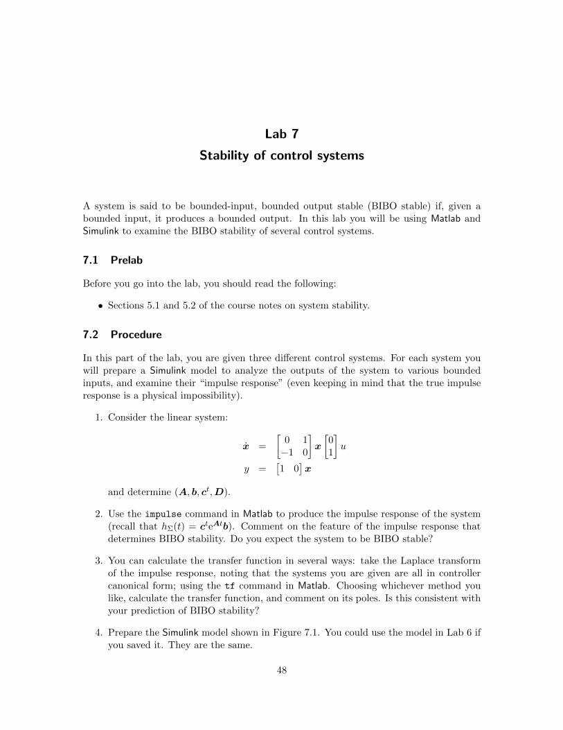
1. Consider the linear system:

x =

[0 1−1 0

]x

[01

]u

y =[1 0

]x

and determine (A, b, ct,D).

2. Use the impulse command in Matlab to produce the impulse response of the system(recall that hΣ(t) = cteAtb). Comment on the feature of the impulse response thatdetermines BIBO stability. Do you expect the system to be BIBO stable?

3. You can calculate the transfer function in several ways: take the Laplace transformof the impulse response, noting that the systems you are given are all in controllercanonical form; using the tf command in Matlab. Choosing whichever method youlike, calculate the transfer function, and comment on its poles. Is this consistent withyour prediction of BIBO stability?

4. Prepare the Simulink model shown in Figure 7.1. You could use the model in Lab 6 ifyou saved it. They are the same.

48

7.2. PROCEDURE 49


5. If you determined that the system is not BIBO stable, modify your Simulink model byreplacing the Pulse Generator with the Fcn block and specifying a bounded inputthat will produce an unbounded output. If the system was determined to be BIBOstable, give the system any bounded input you desire. In either case, print a plot ofthe output variable y and the input variable u.

6. We will now examine the impulse response of the system. You can use thesame Simulink model generated above and proceed as in Lab 6. Recall that thePulse Generator block introduced the impulse function

uε(t) =

{1ε , t ≤ ε,0, otherwise

at every specified period.

Run the Simulink model with the initial conditions set to zero. The default fi-nal time is set to 10s by Simulink. You may change it by opening the win-dow Simulation→Configuration Parameters and entering the desired time in theStop Time box. Larger stop times may be useful here. Reduce the value of ε until yousee no further change in the process response. Show at least three impulse responsesusing different values of ε and note the changes between them.

7. Repeat the procedure for the following two models:

x =

[0 1−2 −3

]x +

[01

]u

y =[1 2

]x

50 LAB 7. STABILITY OF CONTROL SYSTEMS

and

x =

[0 14 −3

]x +

[01

]u

y =[0 1

]x.

8. In Lab 6 you examined the impulse response of the motor system when the outputof the system was the motor angle, θ, and the motor velocity, ω. Using the data yougathered in that lab, comment on the BIBO stability of both systems, commentingon the impulse response, and poles of the function.

When you have completed the lab, make sure you save your files in the folder youcreated in Lab 1.

Lab 8

The Nyquist criterion

In this lab, you will use the Nyquist contour to determine if a system is IBIBO stable. TheNyquist plot is a conformal mapping of a closed loop in complex plane and it is a tool forthe understanding of the stability of a closed-looped system. Furthermore, you will be ex-amining the relationship between the Nyquist contour and the Bode plot, thus familiarizingyourself with such terms as crossover frequency , gain margin, and phase margin.

8.1 Prelab


• Sections 7.1.2 and 7.2 from the course text on the Nyquist criterion.

8.2 Procedure

8.2.1 Using the Bode plot to sketch the Nyquist contour

For this part of the lab, we will be using the motor in the unity gain feedback configurationshown in Figure 8.1. This setup should be quite familiar to you by now, so you should

θd(s) - f+ - RC(s) - RP (s) - θ(s)6


have a well-developed intuition concerning the IBIBO stability of such a system. We will betaking the output of the system to be the motor velocity, ω, so our plant transfer functionis RP (s) = kE

s+ 1τ

. In Lab 2 you constructed the Bode plot for this system experimentally.

1. Using the Bode plot from Lab 2, determine the gain and phase crossover frequencies,and the phase and gain margins at these frequencies; see Section 7.2.2 from the coursetext.

2. Using the Bode plot determine the general transfer function, from the transfer functionsketch the corresponding Nyquist contour. Looking also at the transfer function,determine whether or not the system is IBIBO stable.

51

52 LAB 8. THE NYQUIST CRITERION

3. Start up Matlab and define t to be the transfer function of the open-loop motorscheme. Essentially, we are just setting RC(s) = 1 to see how motor behaves on itsown.

4. To plot the Nyquist contour, use the Nyquist command in Matlab.

5. Is the Nyquist contour consistent with what you know about the IBIBO stability ofthe system? Comment on both the poles of the transfer function, and the zeroes ofthe characteristic polynomial.

8.2.2 Using a proportional controller

We will now turn our attention to the task of using the Nyquist contour as a tool indetermining what range of values of a proportional controller can take on in order to makethe system IBIBO stable.

The plant transfer function RC(s) = K will be used in the feedback configurationdepicted in Figure 8.1. The transfer function for this system is simply

T (s) =KRP (s)

1 +KRP (s).

What is important to note is that the condition KRP (s) = −1 is equivalent to the conditionRP = − 1

K . This seems obvious in itself, but what this allows you to do is to use the Nyquistcontour for RP (s) on its own (i.e., with K = 1), and determine where you would like thepoint 1

K to be. This allows you to get a lot of mileage out of only one plot. The alternativeis to construct the Nyquist contour for many values of K, and see if each contour hasthe required number of encirclements of the point −1 + i0. This may not seem like a badalternative if you have access to a computer, but the method of normalizing the proportionalgain is much more efficient.

1. In Matlab, define the plant transfer function to be RP = s+1s( s

10−1) .

2. Produce both the Bode plot and the Nyquist contour. Take a minute to furtherreaffirm your faith in the relationship between the two.

3. What are the crossover frequencies, and what are the gain and phase margins at thesefrequencies?

4. Since our plant transfer function has one pole in the right-half complex plane, werequire one counterclockwise encirclements of the point 1

K . Using this information, inwhich region should we place the point − 1

K ?

5. What values of K satisfy the above requirement?

6. Repeat the above procedure for the plant transfer function RP (s) = 1s(s+1)2

. Remem-

ber, Nyquist plots always close clockwise.

8.2. PROCEDURE 53

8.2.3 The phase margin

In this part of the lab we will quickly demonstrate the phase margin as it applies to theNyquist contour.

1. We will use the plant transfer function RP (s) = 1s(s+1)2

. Produce the Bode plot and

the Nyquist contour of this system.

2. Determine how much you have to boost the gain (in decibels) to provide a phasemargin of 80◦ at a gain cross over frequency of 10n rad

sec , n ∈ Z. Will the resultingsystem, with this gain boosted by using a proportional controller, be IBIBO stable?

3. The number you get is a scalar that represents the factor by which you can “stretch”(or “shrink” as the case may be) the Nyquist contour towards the point −1 + i0 andstill maintain IBIBO stability (assuming the system is stable for K = 1, which oursystem is). Looking at the Nyquist contour, does this scalar quantity seem to makesense? Is this consistent with your work from Section 8.2.1?


Lab 9

PID design using frequency response

In this lab, you will use the Bode plot you produced using the measurements for the motorto design a PID controller to meet specified performance criteria.

9.1 Prelab


• Section 12.2 from the course text on using frequency response method for controllerdesign.

Since Simulink does not allow improper transfer functions, you must use the PID block forthe controller in this lab. Find the relationships between the constants in equation (9.1)and (9.2):

K

s(1 + TDs)(s+

1

TI), (9.1)

P +I

s+Ds. (9.2)

9.2 Procedure

Before we implement the controller, we need to do some paper work to design it.

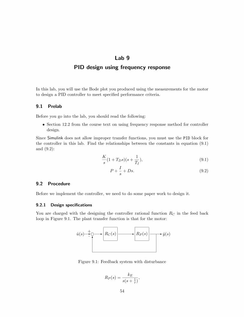
9.2.1 Design specifications

You are charged with the designing the controller rational function RC in the feed backloop in Figure 9.1. The plant transfer function is that for the motor:

u(s) - f+ - RC(s) - RP (s) - y(s)6


RP (s) =kE

s(s+ 1τ ),

54

9.2. PROCEDURE 55

where you have measured the values for kE and τ in Lab 1.You are asked to design a controller so that the closed-loop system has a phase margin

of 65◦ and a crossover frequency as large as possible. The controller you will use is a PIDcontroller in the form

RC(s) =K

s(1 + TDs)(s+

1

TI) = K(1 +

TDTI

+ TDs+1

TIs).

9.2.2 The steps in controller design

We shall lead you by hand through the design process.

1. Produce the Bode plot for plant transfer function using Matlab.

2. In the PID controller design, let us decide to fix TI = 10TD. You are free to changethis ratio during the lab if you find it unsuitable.

3. Also, to start the design process, let us fix the gain K to 1. You may want to use thezpk function in Matlab to define the transfer function.

4. With the above assumptions, is it true that there is a choice for TD for which theclosed loop system is IBIBO stable (IBIBO stability can be verified either by NyquistCriterion or Hurwitz Criterion)? Is it true that, no matter what choice one makes forTD, the closed-loop system will be IBIBO stable? Can you spot the features on yourBode and/or Nyquist plot which help you answer this question? How do these play arole in the design of the controller?

5. Based upon the considerations in the previous step, choose a value for TD which meetsthe design objectives.

6. Now choose K to give the crossover frequency.

7. Make sure the closed-loop system is IBIBO stable using the Nyquist criterion.

You now have values for K, TD, and TI which you will carry into the rest of theprocedure.

9.2.3 Executing the design in hardware/software

Now you will implement your controller in hardware.

1. Open Matlab and build a Simulink model according to Figure 9.2.

2. Use values for K, TD, and TI that make the closed loop system unstable in hardware.Use the above contraints you just calculated to determine values that cause instability.Be prepare to shut the system off! Produce plots of the unstable system.

3. Now, using an input step response of 1, use the “good” values for K, TD, and TI todetermine the rise time, the percentage overshoot, and the ε-settling time for ε = 0.5.

56 LAB 9. PID DESIGN USING FREQUENCY RESPONSE

Figure 9.2: Simulink model for the implementation of PID control using frequency responsemethod; step reference

4. Now run the system with your “good” values for K, TD, and TI and a sinusoidalinput whose magnitude is 1 and whose frequency is the crossover frequency that wascalculated above; see Figure 9.3 for the Simulink. What is the magnitude of the outputcompared to the input, and what is the phase of the output relative to the input?

5. Is your controller a good one? How might you improve it? What do your improvementsmean in terms of loopshaping ideas?

6. Change the ratio of TITD

and discuss the effect on the performance of the controller.Does what you observe make sense? Generate plots to demonstrate your observations.


9.2. PROCEDURE 57

Figure 9.3: Simulink model for the implementation of PID control using frequency responsemethod; sinusoidal reference

Appendix A

Matlab

The students of this course should be familiar with the basic ideas of computer programmingand Matlab from first year courses.

A.1 Defining variables

• x=3

Defines the variable x to be the constant 3.

• x=(1,2;3,4;5,6)

Defines the variable x to be the 3× 2 matrix1 23 45 6

Elements of a row are delimited by commas (or spaces) and each row is delimited bya semicolon.

A.2 General Commands

• dir

Displays a list of files in the current directory.

• open lab_1.mdl

Opens the specific file in the argument. We will be dealing mostly with *.mdl and*.m files.

• who

Displays a list of variables in the memory of Matlab.

• simulink

Opens the Simulink Browser Library window. Using the GUI control, you can dragand drop the blocks to build the Simulink models needed for each lab. Details on usingSimulink and WinCon are discussed in Appendix B.

58

A.3. PLOTTING 59

A.3 Plotting

• plot (lab_1_Tachometer)

Plots the data from the variable lab_1_Tachometer in Matlab memory. You can checkthe list of variables in the Matlab memory by using the who command.

• plot (lab_1_Tachometer,’r:’)

Plots the result in the memory of Matlab and specifies the colour of the graph to bered and the line style to be dotted. Colour and line format are optional commandsand they do not have to be specified for the plot command to produce an output. Youcan also specify one style parameter without the other. The default colour is blue andthe default line style is solid. Table A.1 is a list of colours and line styles that can beused with the plot command.

Line style/colour Matlab command

solid ’-’

dashed ’--’

dotted ’:’

dash-dot ’-.’

blue ’b’ or ’blue’

black ’k’ or ’black’

cyan ’c’ or ’cyan’

green ’g’ or ’green’

magenta ’m’ or ’magenta’

red ’r’ or ’red’

white ’w’ or ’white’

yellow ’y’ or ’yellow’

Table A.1: Colour commands in Matlab

• title (’Angular Velocity of the Motor’)

Sets the title of the plot to the text in quotations.

• xlabel (’Time (s)’)

Sets the x-axis label of the plot to the text in quotations.

• ylabel (’rad/sec’)

Sets the y-axis label of the plot to the text in quotations.

• hold

Hold the current graph in figure and allow the user to plot more than one set of dataon the same figure.

• hold off

Release the current graph in figure and allow a new plot to replace the current graph.

60 APPENDIX A. MATLAB

A.4 Control System Toolbox

• sys = ss(A,b,c,D)

Defines the the state-space system from matrices A, b, c, and D. For a model withn states and 1 output,

– A is an n× n matrix,

– b is an n× 1 matrix,

– c is a 1× n matrix (ct in our notation), and

– D = [0] (always true for this class).

• h = tf([1 0],[1 2 10])

Defines the variable h to be the transfer function

s

s2 + 2s+ 10.

• h = zpk([1 0],[-1 -2 -10],[3])

Defines the variable h to be the transfer function using the location of the zeros, poles,and a multiplicative constant:

3s(s− 1)

(s+ 1)(s+ 2)(s+ 10).

• h = tf(sys)

Defines the variable h to be the transfer function for a given state-space system.

• sys = tf2ss[tf]

Gives the SISO linear system corresponding to the transfer function tf.

• bode(sys)

Produces the Bode plots for the given system.

• impulse(sys)

Produces the impulse response for the given system.

• nyquist(sys)

Produces the Nyquist plot for the given system.

• margin(sys)

Produces the gain and phase margins with associated crossover frequencies.

Appendix B

Simulink

Simulink allows simulation of complex control systems using a drag and drop block dia-gram interface. Simulink is especially useful when used in conjunction with the Real-TimeWorkshop which allows Simulink diagrams to be converted into C codes which can be runin real-time on a number of so-called targets (the PC being one such target).

B.1 Starting

• To use Simulink, one must first start Matlab. After starting Matlab, you would typesimulink in the Matlab command prompt to get the Simulink Library Browser

window.

• Selecting File→New→Model (or Ctrl+N) while in the Simulink Library Browser

will give you a blank model window into which you can drag-and-drop system blocksfrom the Simulink Library Browser to build a Simulink model. These models canbe saved as *.mdl files for future simulations and editing.

B.2 Building a Simulink model

• To connect the output of block A to the input of block B, simply left-click the outputport of block A and drag the line that would appear into the input port of the block B.

• In order to connect the output of a block into the inputs of multiple blocks at thesame time, you can right-click on an existing connection to get another line and dragthat connection into the input of another block.

• When a block is dragged into the model window, it will be given a generic name. Forexample, when the scope block is dragged into a model, it would simply be labelledas “scope” and if it was the second scope block to be dragged into the model, it wouldbe labelled as “scope2”. It is a good practice to rename these blocks and give themmore appropriate labels. These names are usually suggested in the diagram of themodels in each lab. To rename a block, simply click on the existing name once andedit.

B.3 Simulations

• One could view and edit the simulation parameters by clicking on

61

62 APPENDIX B. SIMULINK

Simulation→Simulation Parameters

(or Ctrl+E) while editing the model. For the purpose of this course, there are onlythree things that you have to worry about:

1. Start and stop time: The default start time is 0 and the default stop time is 10.Usually, there is no reason to change the default start time, but you might findit useful to extend the stop time so that you could observe the simulation for alonger period of time.

2. Solver Method: You must have this set to a fixed-step when implementing real-time controllers. The default solver is a discrete method. You need to change itfrom the default method to ode4, which is an implementation of the Runge-Kuttamethod.

3. Step size: The default setting of 0.001 corresponds to 1000 Hz sampling fre-quency. This is the fastest rate at which the system can sample.

B.4 Plotting

• The outputs of a simulation can be captured by using the To Workspace block. Thedata would be recorded as a variable in memory of Matlab. The default name of theoutput is simout, but you should change the name of this output just as you wouldgive appropriate label to the block itself. One could plot the simulation output byusing plot command discussed in Appendix A.

B.4.1 Saving data via the “To Workspace” block

This is the preferred method of saving data to your Matlab workspace. The To Workspace

block can be found at

Simulink→Sinks

Drag this block into your workspace and connect it to the variable you wish to save. Doubleclick on the block to configure it. Choose a good variable name and in the save format

drop down menu select Structure with time. After the simulation the data will be auto-matically saved to your Matlab workspace and you can plot it with the command

plot(varname.time,varname.signals.values)

replacing “varname” with the variable name you chose when configuring the To Workspace

block.

B.4.2 Saving data from a scope

You can also save scope data, but the scope seems to have short-term memory loss whichmakes it one of the most useless blocks in the simulink library. Nevertheless if you need tosave the data from a scope, follow these instructions.

B.4. PLOTTING 63

1. Double click on the scope you wish to save the data from.

2. Click on the Parameters Icon (in the top left of the scope dialog box).

3. Data History Tab

• Uncheck box Limit data points

• Check box Save data to workspace

• Choose a variable name

• Select Array from the Format drop down menu.

4. Click Apply and OK to exit.

After the simulation has been performed, the data will appear as an array in your Matlabworkspace. You can plot the data with the command

plot(ScopeData1(:,1), ScopeData1(:,2))

where ScopeData1 is the variable name that you set in the above steps.

Appendix C

Lab Equipment

In the lab, there are several computers equipped with data acquisition systems runningWindows 7 with Matlab. The hardware equipment and some software tools are manufac-tured by Quanser Consulting, a Canadian company developing real-time control systemsfor education and research. This document introduces some of the hardware equipment tobe used in the labs. Familiarity with this document is needed to perform the labs.

C.1 Hardware devices

The lab hardware consists of three components:

1. data acquisition system;

2. power module;

3. servomotors.

C.2 Data Acquisition Board

In order for the computer to run a controller, analog-to-digital (A/D) and digital-to-analog(D/A) conversions are necessary. These are done using the data acquisition and controlboard (DACB), which inputs the measured signal(s) to the computer and outputs controlaction to the actuator in the control loop. The DACB in this lab consists of a single board:the Q2-USB, which is made by Quanser Consulting. Figure C.1 shows a photo of the Q2-USB card. This data acquisition board is an external board connected to the computerthrough a USB port.

Figure C.1 also shows the proper configuration of the data acquisition board. TheEncoder is the 5 pin Din and is plugged in to channel 0 in the Encoders portion of theboard. The tachometer (S3 on the Quanser) is the red RCA plug and is plugged intochannel 0 is the ADC portion of the board. Finally the analog output is the solo black RCAplug and is plugged in to channel 0 of the DAC portion of the board.

C.3 Universal power module

The universal power module (UPM-2405), which is shown in Figure C.2, is a linear poweroperations amplifier. The Q2-USB data acquisition board cannot deliver enough power tothe actuators used in this lab; therefore, a signal buffer is needed. The UPM-2405 is used

64

http://www.quanser.com/

C.3. UNIVERSAL POWER MODULE 65

Figure C.1: Q2-USB data acquisition board

Figure C.2: Universal power module

66 APPENDIX C. LAB EQUIPMENT

as our signal buffer since it can deliver up to 5A to an actuator in a non-inverting, unitygain configuration.

The following connections can be made to/from the UPM (see the labels on the UPM).

• From analog sensors: there are four (S1-S4 inputs which can be connected from analogsensors (and then subsequently to the computer); the cable used is a 6-pin mini-din/6-pin mini-din cable (light tan colour), which is now referred to as the analog sensorcable.

• To A/D: the four analog sensor signals (S1-S4) can then be connected to the Q2-USB terminal board for A/D conversion into the computer; the cable used is a 5-pindin-stereo/4RCA cable (black colour), which is now referred to as the A/D cables.

• From D/A: this is where you input the D/A signal from the Q2-USB terminal boardto the UPM; the cable used is a 5-pin din-mono/RCA cable (black colour), which isnow referred to as the D/A cable.

• To load: here you connect the amplified D/A signal to an actuator (e.g., servomotor);the cable used is a 7-pin din/4-pin din cable (black colour), which is now referred toas the load cable. Note there are two types of load cables one with unity gain andanother with a cable gain of 5. Make sure you use the right one.

• Others: A few other connections are possible for convenience: e.g., a DC power supplyon the top left provides 12 volts; the signal s from analog sensors S1-S4 can be easilymonitored by connecting to a scope to the banana plug terminals.

C.4 DC servomotor

The Quanser DC servomotor (SRV02) is shown in Figure C.3. A 3W motor is mountedin a solid aluminium frame and drives a built-in Swiss-made 14.1:1 gearbox whose outputdrives an external gear, which is attached to an independent output shaft that rotates in analuminium ball-bearing block. The output shaft is equipped with an encoder. The externalgear on the output shaft drives an anti-backlash gear connected to a precision potentiometerfor measuring the output angle. The external gear ratio can be changed from 1:1 to 5:1using different gears. Two inertial loads are supplied with the system in order to examinethe effect of changing inertia on motor performance. Several connections are availablefor the servomotor. The input voltage connects to the UPM using the load cable. Thepotentiometer and tachometer ports connect to the UPM-2405 using sensor cables and areused to measure angular position and angular velocity respectively. Additionally, the shaftencoder port connects to the terminal board using an encoder cable and is used to measureangular position. The calibration factors listed in Table C.1 are needed in order to use thesensors in units of degrees or radians.

C.4. DC SERVOMOTOR 67

Figure C.3: DC servomotor (SRV02)

Connection Conversion (Rad) Conversion(Deg)

Encoder − 2π4096 − 360

4096

Tachometer 1 radsec

100π63

degsec

Potentiometer 14096

1804096π

Table C.1: Conversion factors