Embed Size (px)
Citation preview
© Numerical Factory
Mètodes Numèrics: A First Course on Finite Elements
Dept. Matemàtiques ETSEIB - UPC BarcelonaTech
Finite Elements
Following: Curs d’Elements Finits amb Aplicacions (J. Masdemont)http://hdl.handle.net/2099.3/36166
© Numerical Factory
Finite Elements
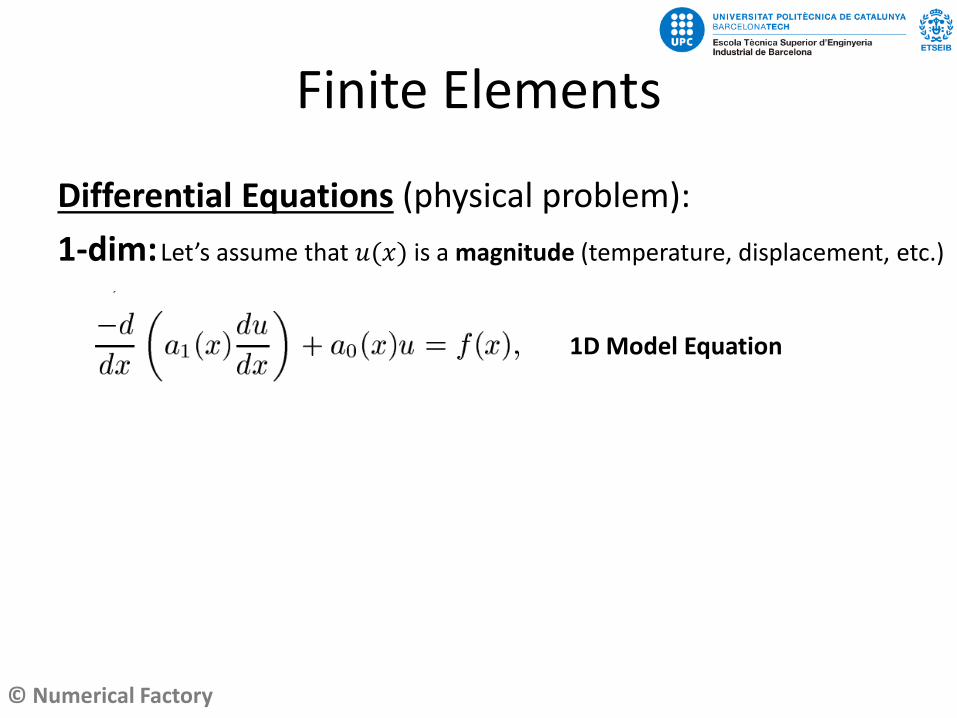
Differential Equations (physical problem):
1-dim:Let’s assume that 𝑢(𝑥) is a magnitude (temperature, displacement, etc.)
1D Model Equation

© Numerical Factory
Finite Elements
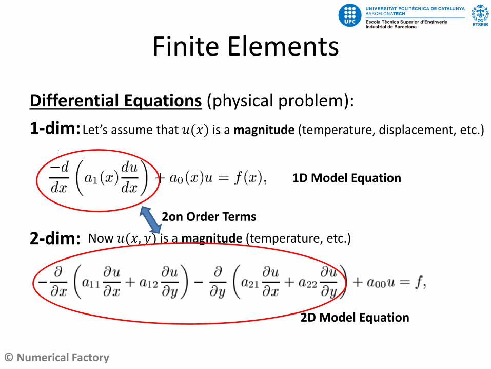
Differential Equations (physical problem):
1-dim:
2-dim:
Let’s assume that 𝑢(𝑥) is a magnitude (temperature, displacement, etc.)
1D Model Equation
Now 𝑢(𝑥, 𝑦) is a magnitude (temperature, etc.)
2D Model Equation
© Numerical Factory
Finite Elements
Differential Equations (physical problem):
1-dim:
2-dim:
Let’s assume that 𝑢(𝑥) is a magnitude (temperature, displacement, etc.)
1D Model Equation
Now 𝑢(𝑥, 𝑦) is a magnitude (temperature, etc.)
2D Model Equation
2on Order Terms
© Numerical Factory
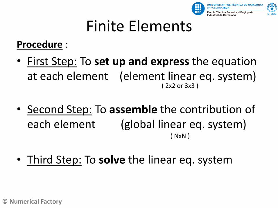
Finite Elements Procedure :
• First Step: To set up and express the equation at each element (element linear eq. system)
• Second Step: To assemble the contribution of each element (global linear eq. system)
• Third Step: To solve the linear eq. system
( 2x2 or 3x3 )
( NxN )

© Numerical Factory
Finite Elements
Finite Elements
Stp1: Discretize in elements
Stp2: Write the variational equations
Stp3: Build the Linear SystemImpose the BC
Stp4: Get nodes solution
Stp5: Extent solution to the Domain
Meshing the domain
© Numerical Factory
Finite Elements
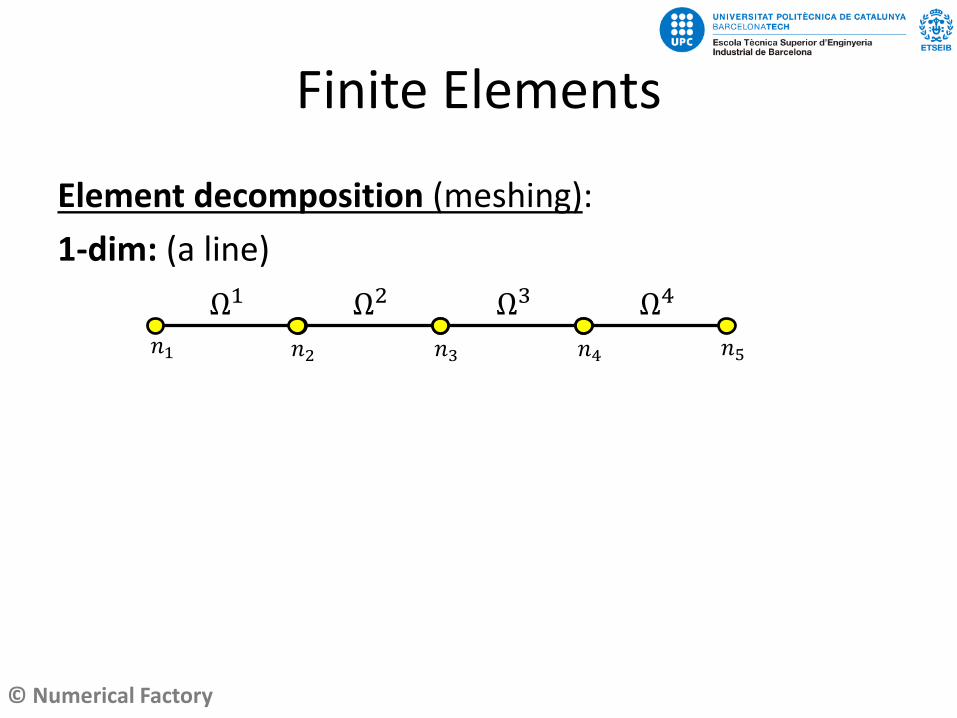
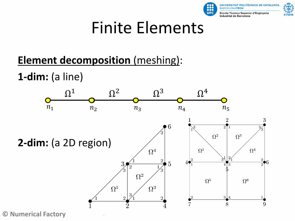
Element decomposition (meshing):
1-dim: (a line)
𝑛2 𝑛3 𝑛4𝑛1
Ω1 Ω2 Ω3 Ω4
𝑛5
© Numerical Factory
Finite Elements
Element decomposition (meshing):
1-dim: (a line)
2-dim: (a 2D region)
𝑛2 𝑛3 𝑛4𝑛1
Ω1 Ω2 Ω3 Ω4
𝑛5
© Numerical Factory
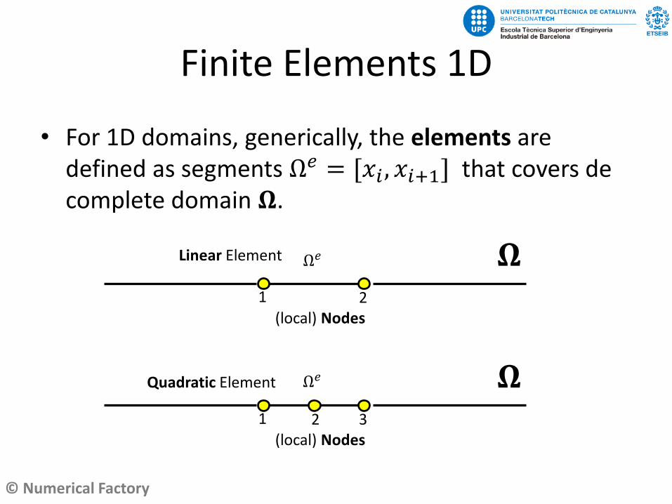
• For 1D domains, generically, the elements are defined as segments Ω𝑒 = [𝑥𝑖 , 𝑥𝑖+1] that covers de complete domain 𝛀.
Finite Elements 1D
(local) Nodes
1 2
Linear Element 𝛀
(local) Nodes
1 2
Quadratic Element 𝛀3
Ω𝑒
Ω𝑒
© Numerical Factory
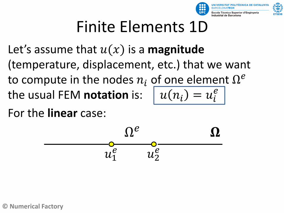
Let’s assume that 𝑢(𝑥) is a magnitude(temperature, displacement, etc.) that we want to compute in the nodes 𝑛𝑖 of one element Ω𝑒
the usual FEM notation is: 𝑢 𝑛𝑖 = 𝑢𝑖𝑒
For the linear case:
Finite Elements 1D
𝛀Ω𝑒
𝑢1𝑒 𝑢2
𝑒
© Numerical Factory
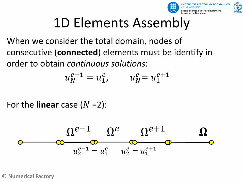
When we consider the total domain, nodes of consecutive (connected) elements must be identify in order to obtain continuous solutions:
𝑢𝑁𝑒−1 = 𝑢1
𝑒, 𝑢𝑁𝑒= 𝑢1
𝑒+1
For the linear case (𝑁 =2):
1D Elements Assembly
𝛀Ω𝑒
𝑢2𝑒−1 = 𝑢1
𝑒
Ω𝑒−1 Ω𝑒+1
𝑢2𝑒 = 𝑢1
𝑒+1
© Numerical Factory
1D Elements Assembly
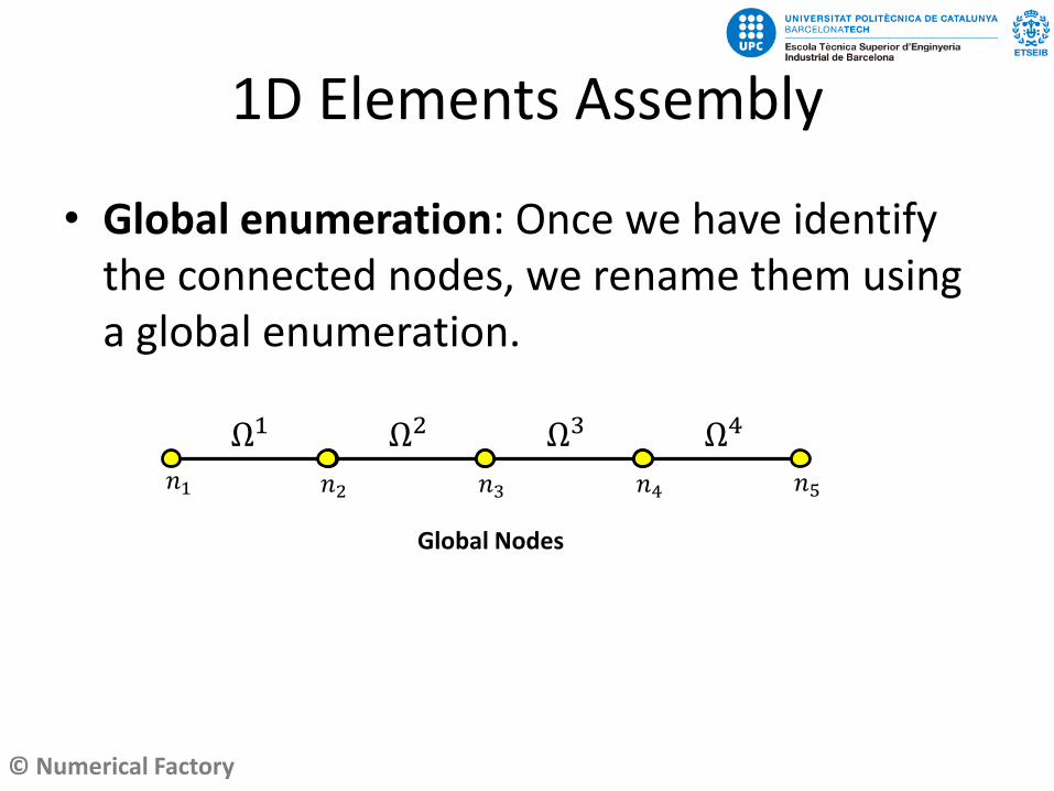
• Global enumeration: Once we have identify the connected nodes, we rename them using a global enumeration.
Global Nodes
𝑛2 𝑛3 𝑛4𝑛1
Ω1 Ω2 Ω3 Ω4
𝑛5
© Numerical Factory
1D Elements Assembly
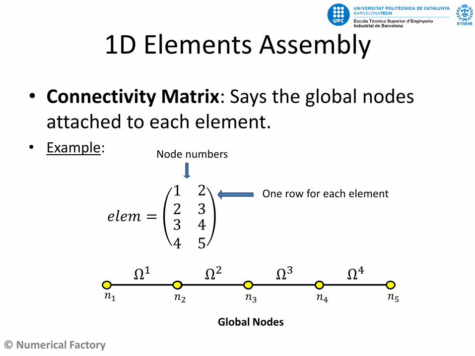
• Connectivity Matrix: Says the global nodes attached to each element.
• Example:
Global Nodes
𝑛2 𝑛3 𝑛4𝑛1
Ω1 Ω2 Ω3 Ω4
𝑛5
𝑒𝑙𝑒𝑚 =
12
23
34
45
One row for each element
Node numbers
© Numerical Factory
1D Elements Assembly
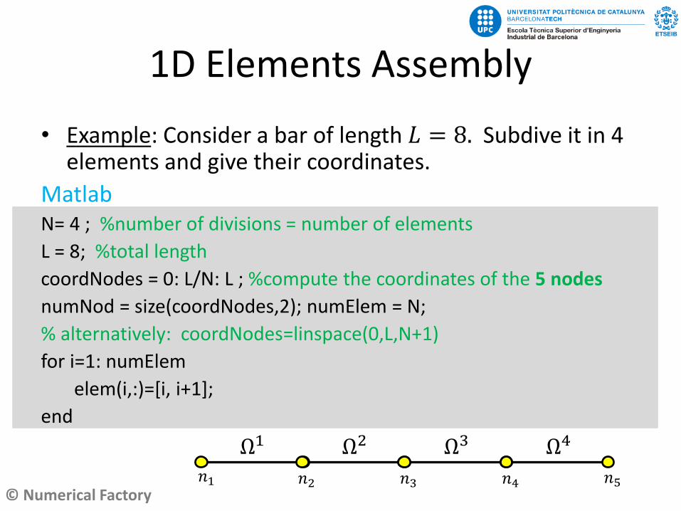
• Example: Consider a bar of length 𝐿 = 8. Subdive it in 4 elements and give their coordinates.
MatlabN= 4 ; %number of divisions = number of elements
L = 8; %total length
coordNodes = 0: L/N: L ; %compute the coordinates of the 5 nodes
numNod = size(coordNodes,2); numElem = N;
% alternatively: coordNodes=linspace(0,L,N+1)
for i=1: numElem
elem(i,:)=[i, i+1];
end
𝑛2 𝑛3 𝑛4𝑛1
Ω1 Ω2 Ω3 Ω4
𝑛5
© Numerical Factory
1D Elements Assembly
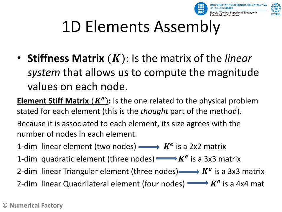
• Stiffness Matrix (𝑲): Is the matrix of the linear system that allows us to compute the magnitude values on each node.
Element Stiff Matrix (𝑲𝒆): Is the one related to the physical problem stated for each element (this is the thought part of the method).
Because it is associated to each element, its size agrees with the number of nodes in each element.
1-dim linear element (two nodes) 𝑲𝒆 is a 2x2 matrix
1-dim quadratic element (three nodes) 𝑲𝒆 is a 3x3 matrix
2-dim linear Triangular element (three nodes) 𝑲𝒆 is a 3x3 matrix
2-dim linear Quadrilateral element (four nodes) 𝑲𝒆 is a 4x4 mat
© Numerical Factory
1D Elements Assembly
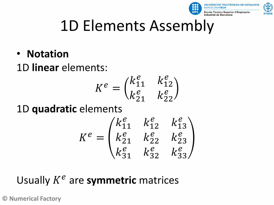
• Notation1D linear elements:
𝐾𝑒 =𝑘11𝑒 𝑘12
𝑒
𝑘21𝑒 𝑘22
𝑒
1D quadratic elements
𝐾𝑒 =
𝑘11𝑒 𝑘12
𝑒 𝑘13𝑒
𝑘21𝑒 𝑘22
𝑒 𝑘23𝑒
𝑘31𝑒 𝑘32
𝑒 𝑘33𝑒
Usually 𝐾𝑒 are symmetric matrices
© Numerical Factory
1D Elements Assembly
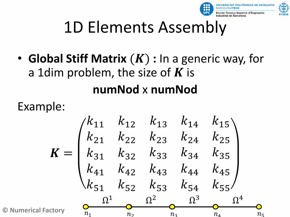
• Global Stiff Matrix (𝑲) : In a generic way, for a 1dim problem, the size of 𝑲 is
numNod x numNod
Example:
𝑲 =
𝑘11𝑘21
𝑘12𝑘22
𝑘13 𝑘14 𝑘15𝑘23 𝑘24 𝑘25
𝑘31 𝑘32 𝑘33 𝑘34 𝑘35𝑘41𝑘51
𝑘42𝑘52
𝑘43 𝑘44 𝑘45𝑘53 𝑘54 𝑘55
𝑛2 𝑛3 𝑛4𝑛1
Ω1 Ω2 Ω3 Ω4
𝑛5
© Numerical Factory
1D Elements Assembly
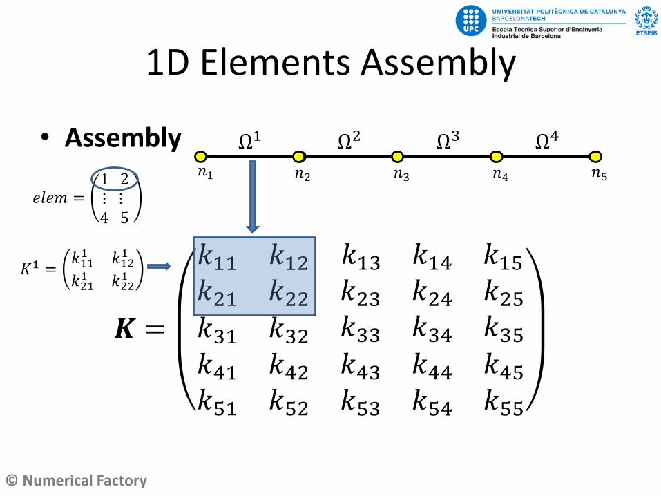
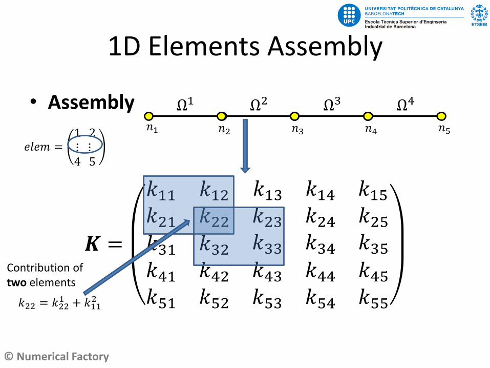
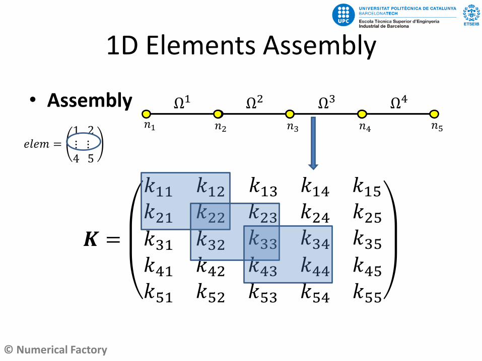
• Assembly
𝑲 =
𝑘11𝑘21
𝑘12𝑘22
𝑘13 𝑘14 𝑘15𝑘23 𝑘24 𝑘25
𝑘31 𝑘32 𝑘33 𝑘34 𝑘35𝑘41𝑘51
𝑘42𝑘52
𝑘43 𝑘44 𝑘45𝑘53 𝑘54 𝑘55
𝑛2 𝑛3 𝑛4𝑛1
Ω1 Ω2 Ω3 Ω4
𝑛5
𝑒𝑙𝑒𝑚 =1⋮4
2⋮5
𝐾1 =𝑘111 𝑘12
1
𝑘211 𝑘22
1
© Numerical Factory
1D Elements Assembly
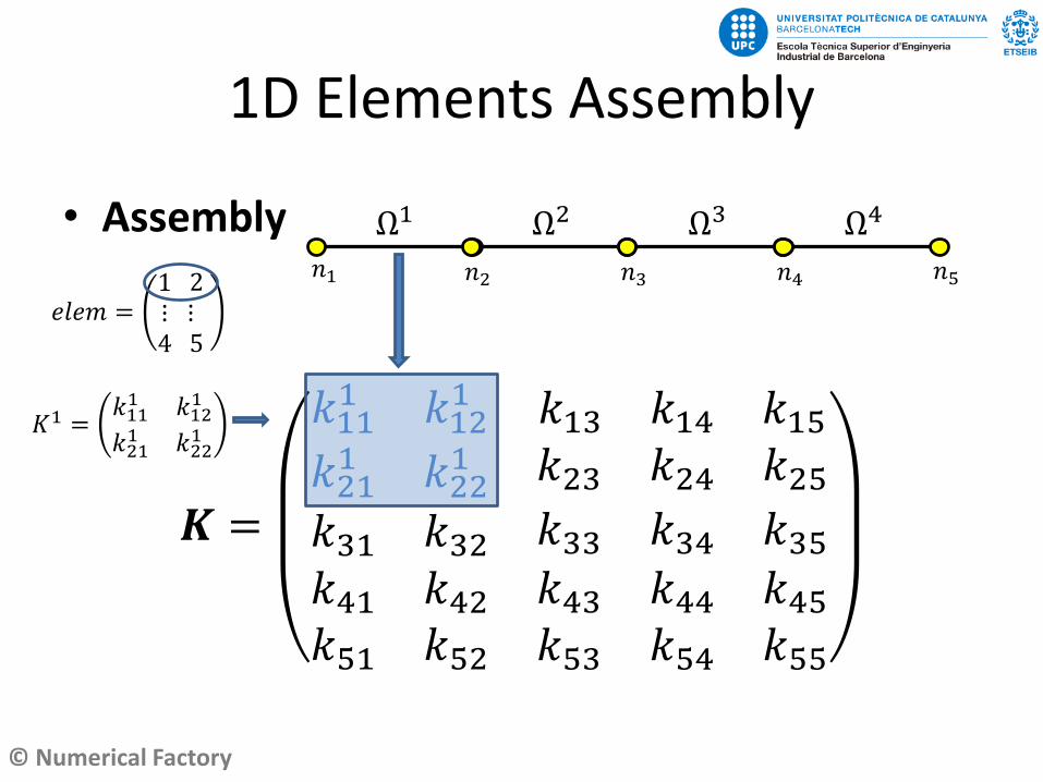
• Assembly
𝑲 =
𝑘111
𝑘211
𝑘121
𝑘221
𝑘13 𝑘14 𝑘15𝑘23 𝑘24 𝑘25
𝑘31 𝑘32 𝑘33 𝑘34 𝑘35𝑘41𝑘51
𝑘42𝑘52
𝑘43 𝑘44 𝑘45𝑘53 𝑘54 𝑘55
𝑛2 𝑛3 𝑛4𝑛1
Ω1 Ω2 Ω3 Ω4
𝑛5
𝑒𝑙𝑒𝑚 =1⋮4
2⋮5
𝐾1 =𝑘111 𝑘12
1
𝑘211 𝑘22
1
© Numerical Factory
1D Elements Assembly
• Assembly
𝑲 =
𝑘11𝑘21
𝑘12𝑘22
𝑘13 𝑘14 𝑘15𝑘23 𝑘24 𝑘25
𝑘31 𝑘32 𝑘33 𝑘34 𝑘35𝑘41𝑘51
𝑘42𝑘52
𝑘43 𝑘44 𝑘45𝑘53 𝑘54 𝑘55
𝑛2 𝑛3 𝑛4𝑛1
Ω1 Ω2 Ω3 Ω4
𝑛5
𝑒𝑙𝑒𝑚 =1⋮4
2⋮5
𝑘22 = 𝑘221 + 𝑘11
2
Contribution of two elements
© Numerical Factory
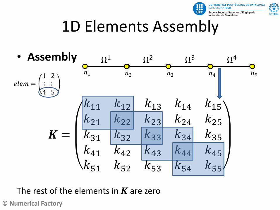
1D Elements Assembly
• Assembly
𝑲 =
𝑘11𝑘21
𝑘12𝑘22
𝑘13 𝑘14 𝑘15𝑘23 𝑘24 𝑘25
𝑘31 𝑘32 𝑘33 𝑘34 𝑘35𝑘41𝑘51
𝑘42𝑘52
𝑘43 𝑘44 𝑘45𝑘53 𝑘54 𝑘55
𝑛2 𝑛3 𝑛4𝑛1
Ω1 Ω2 Ω3 Ω4
𝑛5
𝑒𝑙𝑒𝑚 =1⋮4
2⋮5
© Numerical Factory
1D Elements Assembly
• Assembly
𝑲 =
𝑘11𝑘21
𝑘12𝑘22
𝑘13 𝑘14 𝑘15𝑘23 𝑘24 𝑘25
𝑘31 𝑘32 𝑘33 𝑘34 𝑘35𝑘41𝑘51
𝑘42𝑘52
𝑘43 𝑘44 𝑘45𝑘53 𝑘54 𝑘55
The rest of the elements in 𝑲 are zero
𝑛2 𝑛3 𝑛4𝑛1
Ω1 Ω2 Ω3 Ω4
𝑛5
𝑒𝑙𝑒𝑚 =1⋮4
2⋮5
© Numerical Factory
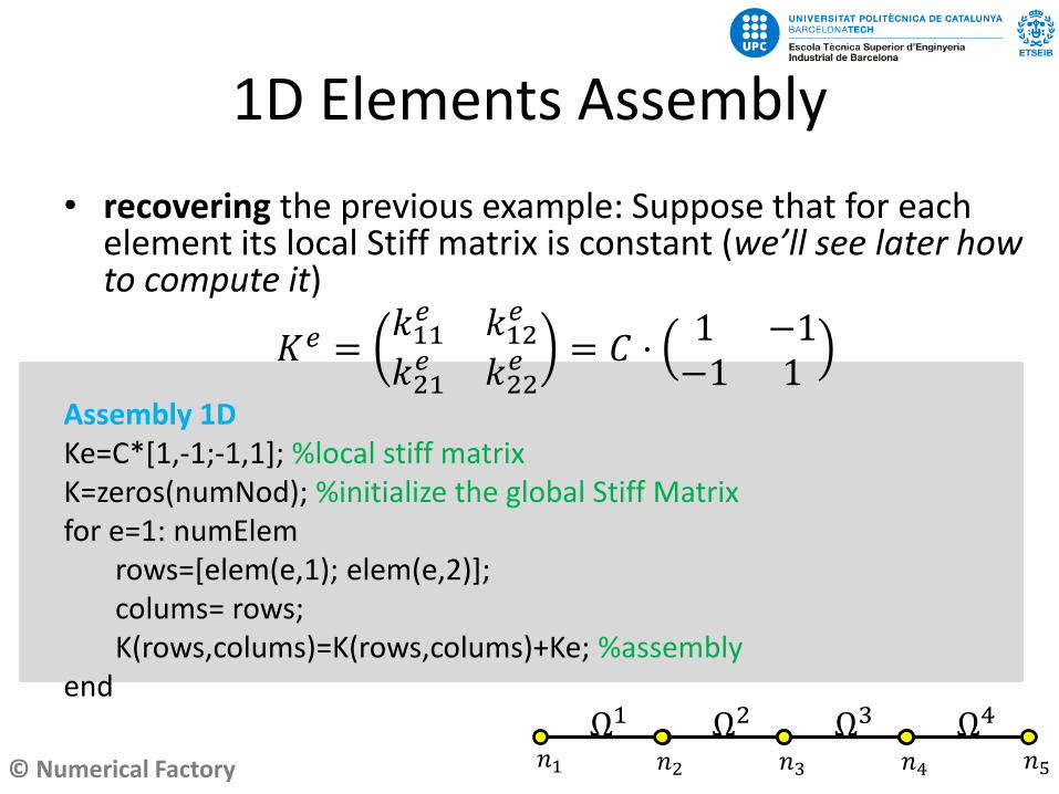
1D Elements Assembly
• recovering the previous example: Suppose that for each element its local Stiff matrix is constant (we’ll see later how to compute it)
𝐾𝑒 =𝑘11𝑒 𝑘12
𝑒
𝑘21𝑒 𝑘22
𝑒 = 𝐶 ·1 −1−1 1
Assembly 1DKe=C*[1,-1;-1,1]; %local stiff matrixK=zeros(numNod); %initialize the global Stiff Matrixfor e=1: numElem
rows=[elem(e,1); elem(e,2)];colums= rows;K(rows,colums)=K(rows,colums)+Ke; %assembly
end
𝑛2 𝑛3 𝑛4𝑛1
Ω1 Ω2 Ω3 Ω4
𝑛5
© Numerical Factory
1D Elements Assembly
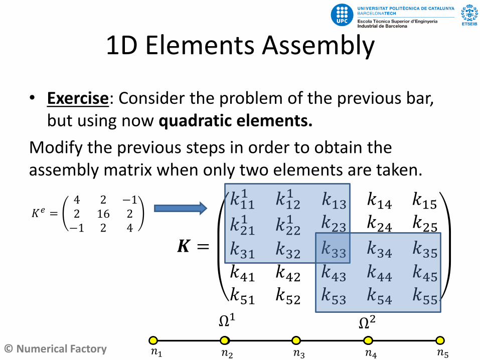
• Exercise: Consider the problem of the previous bar, but using now quadratic elements.
Modify the previous steps in order to obtain the assembly matrix when only two elements are taken.
𝑛2 𝑛3 𝑛4𝑛1
Ω1Ω2
𝑛5
𝐾𝑒 =4 2 −12 16 2−1 2 4
𝑲 =
𝑘111
𝑘211
𝑘121
𝑘221
𝑘13 𝑘14 𝑘15𝑘23 𝑘24 𝑘25
𝑘31 𝑘32 𝑘33 𝑘34 𝑘35𝑘41𝑘51
𝑘42𝑘52
𝑘43 𝑘44 𝑘45𝑘53 𝑘54 𝑘55
© Numerical Factory
2D Elements Assembly
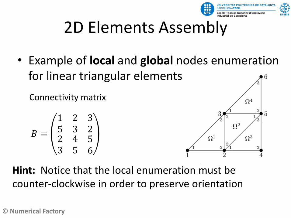
• Example of local and global nodes enumeration for linear triangular elements
Connectivity matrix
𝐵 =
1523
2345
3256
Hint: Notice that the local enumeration must becounter-clockwise in order to preserve orientation
© Numerical Factory
2D Elements Assembly
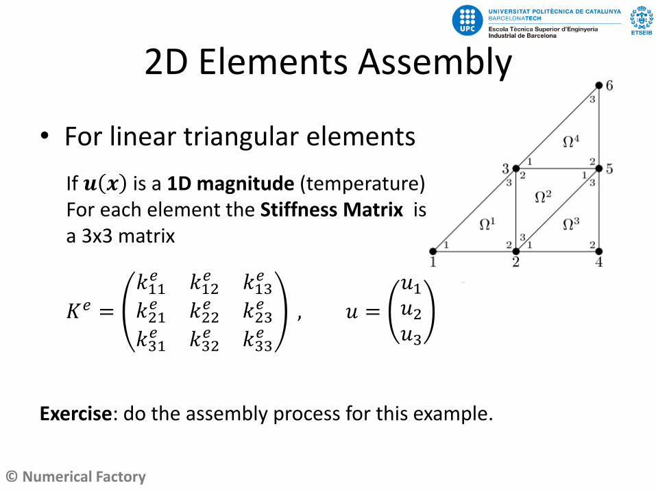
• For linear triangular elements
Exercise: do the assembly process for this example.
If 𝒖 𝒙 is a 1D magnitude (temperature)For each element the Stiffness Matrix isa 3x3 matrix
𝐾𝑒 =
𝑘11𝑒 𝑘12
𝑒 𝑘13𝑒
𝑘21𝑒 𝑘22
𝑒 𝑘23𝑒
𝑘31𝑒 𝑘32
𝑒 𝑘33𝑒
, 𝑢 =
𝑢1𝑢2𝑢3
© Numerical Factory
2D Elements Assembly
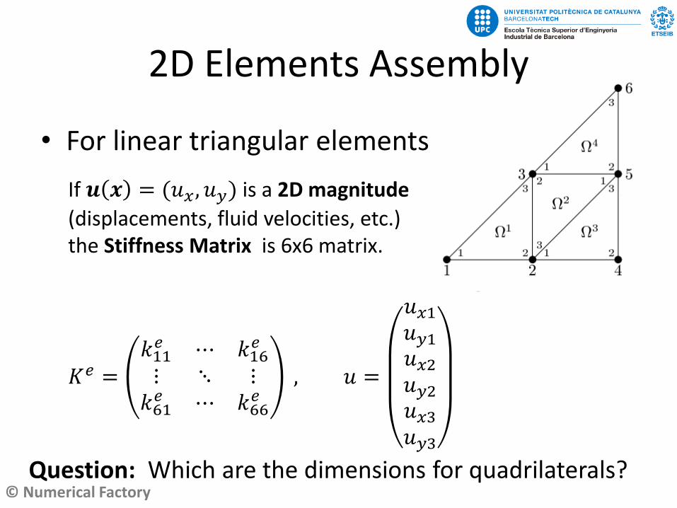
• For linear triangular elements
If 𝒖 𝒙 = (𝑢𝑥 , 𝑢𝑦) is a 2D magnitude
(displacements, fluid velocities, etc.)the Stiffness Matrix is 6x6 matrix.
𝐾𝑒 =𝑘11𝑒 ⋯ 𝑘16
𝑒
⋮ ⋱ ⋮𝑘61𝑒 ⋯ 𝑘66
𝑒, 𝑢 =
𝑢𝑥1𝑢𝑦1𝑢𝑥2𝑢𝑦2𝑢𝑥3𝑢𝑦3
Question: Which are the dimensions for quadrilaterals?
© Numerical Factory
Meshing 2D domains
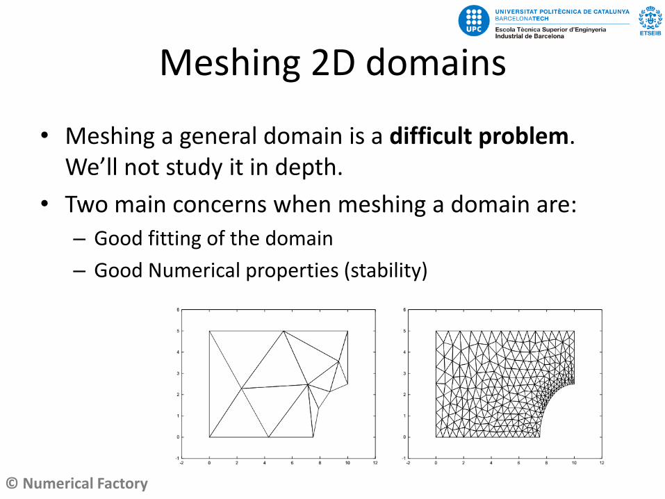
• Meshing a general domain is a difficult problem. We’ll not study it in depth.
• Two main concerns when meshing a domain are:
– Good fitting of the domain
– Good Numerical properties (stability)
© Numerical Factory
Meshing 2D domains
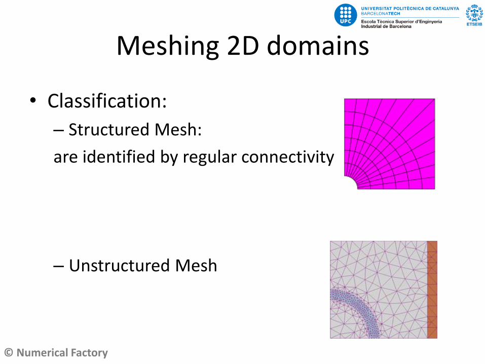
• Classification:
– Structured Mesh:
are identified by regular connectivity
– Unstructured Mesh
© Numerical Factory
Meshing 2D domains
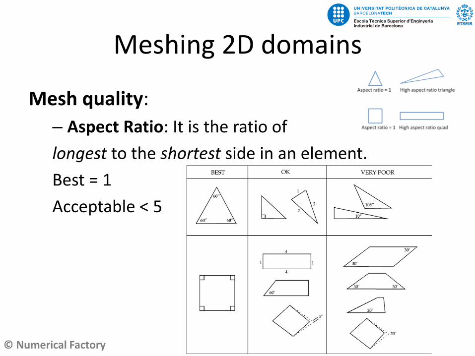
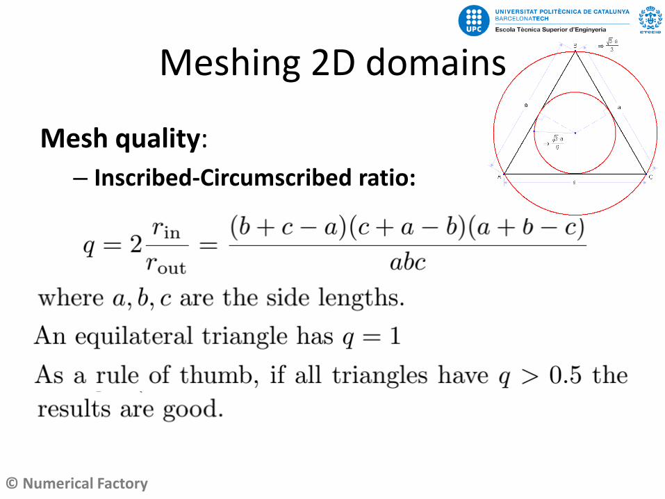
Mesh quality:
– Aspect Ratio: It is the ratio of
longest to the shortest side in an element.
Best = 1
Acceptable < 5
© Numerical Factory
Meshing 2D domains
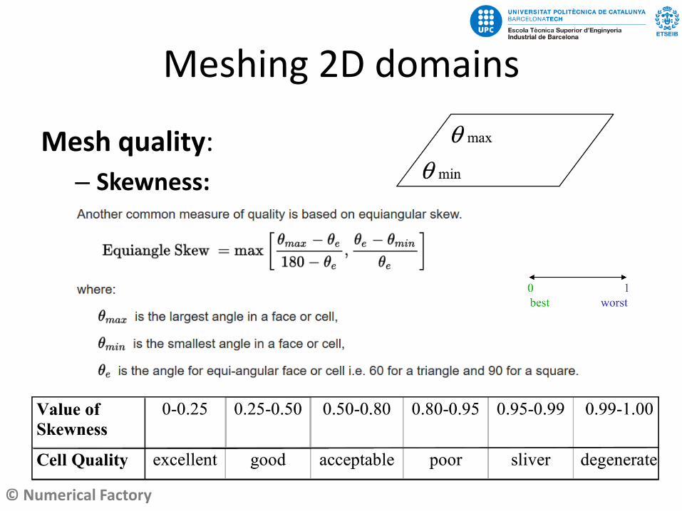
Mesh quality:
– Skewness:
© Numerical Factory
Meshing 2D domains
Mesh quality:
– Inscribed-Circumscribed ratio:
© Numerical Factory
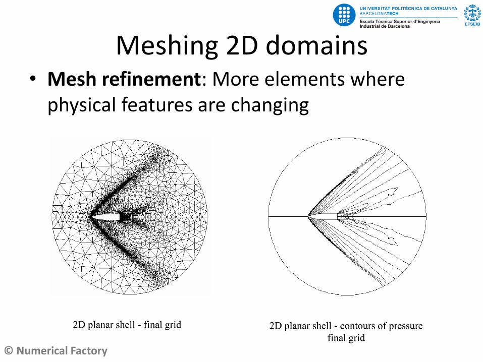
Meshing 2D domains• Mesh refinement: More elements where
physical features are changing

© Numerical Factory
2D-Finite Elements
Finite Elements
Stp1: Discretize in elements
Stp2: Write the variational equations
Stp3: Build the Linear SystemImpose the BC
Stp4: Get nodes solution
Stp5: Extent solution to the Domain
Weak form
© Numerical Factory
2D-Model Equation
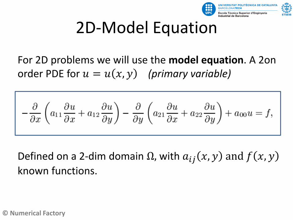
For 2D problems we will use the model equation. A 2on order PDE for 𝑢 = 𝑢 𝑥, 𝑦 (primary variable)
Defined on a 2-dim domain Ω, with 𝑎𝑖𝑗 𝑥, 𝑦 and 𝑓 𝑥, 𝑦
known functions.
© Numerical Factory
2D-Model Equation
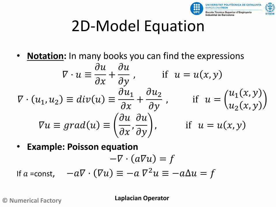
• Notation: In many books you can find the expressions
𝛻 · 𝑢 ≡𝜕𝑢
𝜕𝑥+𝜕𝑢
𝜕𝑦, if 𝑢 = 𝑢 𝑥, 𝑦
𝛻 · 𝑢1, 𝑢2 ≡ 𝑑𝑖𝑣 𝑢 ≡𝜕𝑢1𝜕𝑥
+𝜕𝑢2𝜕𝑦
, if 𝑢 =𝑢1(𝑥, 𝑦)
𝑢2 𝑥, 𝑦
𝛻𝑢 ≡ 𝑔𝑟𝑎𝑑 𝑢 ≡𝜕𝑢
𝜕𝑥,𝜕𝑢
𝜕𝑦, if 𝑢 = 𝑢 𝑥, 𝑦
• Example: Poisson equation−𝛻 · 𝑎𝛻𝑢 = 𝑓
If 𝑎 =const, −𝑎𝛻 · 𝛻𝑢 ≡ −𝑎 𝛻2𝑢 ≡ −𝑎∆𝑢 = 𝑓
Laplacian Operator
© Numerical Factory
2D-Model Equation
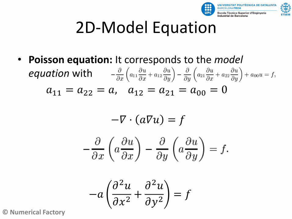
• Poisson equation: It corresponds to the model equation with
𝑎11 = 𝑎22 = 𝑎, 𝑎12 = 𝑎21 = 𝑎00 = 0
−𝛻 · 𝑎𝛻𝑢 = 𝑓
−𝑎𝜕2𝑢
𝜕𝑥2+𝜕2𝑢
𝜕𝑦2= 𝑓
© Numerical Factory
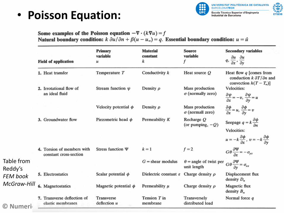
• Poisson Equation:
Table fromReddy’s FEM bookMcGraw-Hill
© Numerical Factory
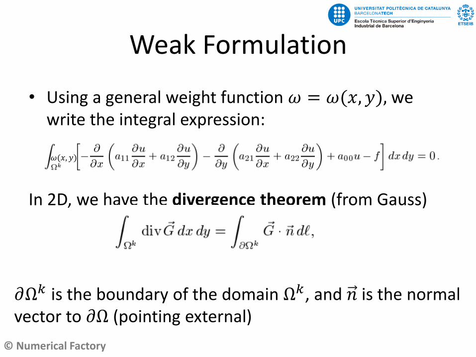
Weak Formulation
• Using a general weight function 𝜔 = 𝜔(𝑥, 𝑦), we write the integral expression:
In 2D, we have the divergence theorem (from Gauss)
𝜕Ω𝑘 is the boundary of the domain Ω𝑘, and 𝑛 is the normal vector to 𝜕Ω (pointing external)
𝜔(𝑥, 𝑦)
© Numerical Factory
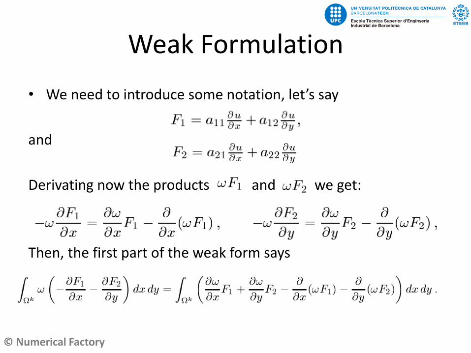
Weak Formulation
• We need to introduce some notation, let’s say
and
Derivating now the products and we get:
Then, the first part of the weak form says
© Numerical Factory
Weak Formulation
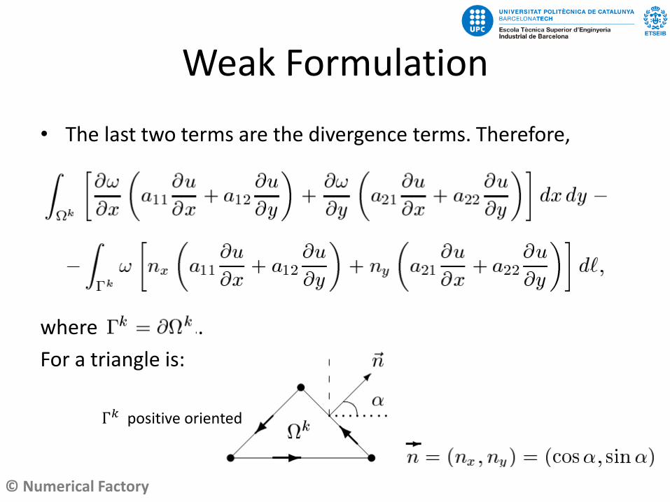
• The last two terms are the divergence terms. Therefore,
where .
For a triangle is:
Γ𝑘 positive oriented
© Numerical Factory
Weak Formulation
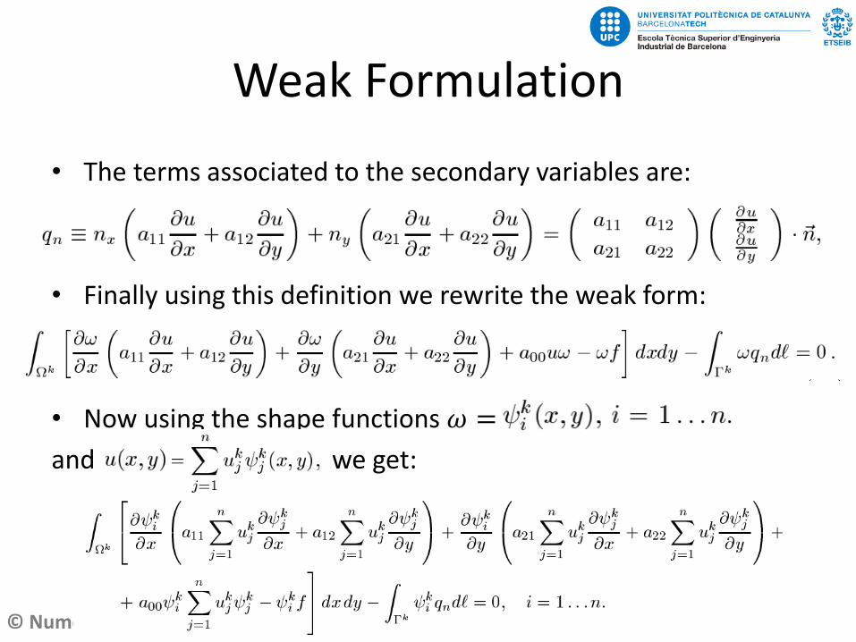
• The terms associated to the secondary variables are:
• Finally using this definition we rewrite the weak form:
• Now using the shape functions 𝜔 =
and we get:

© Numerical Factory
Weak Formulation
• Grouping the unknown terms
or, as a linear system

© Numerical Factory
Notation:
𝑢 = 𝑢(𝑥, 𝑦) is named primary variable
is named secondary variable
Boundary Conditions (BC):
𝑢𝐴 = 𝑢(𝑥𝐴) is an essential BC (fix the primary variable)
is a natural BC (fix the secondary variable)
Weak Formulation
© Numerical Factory
Weak Formulation
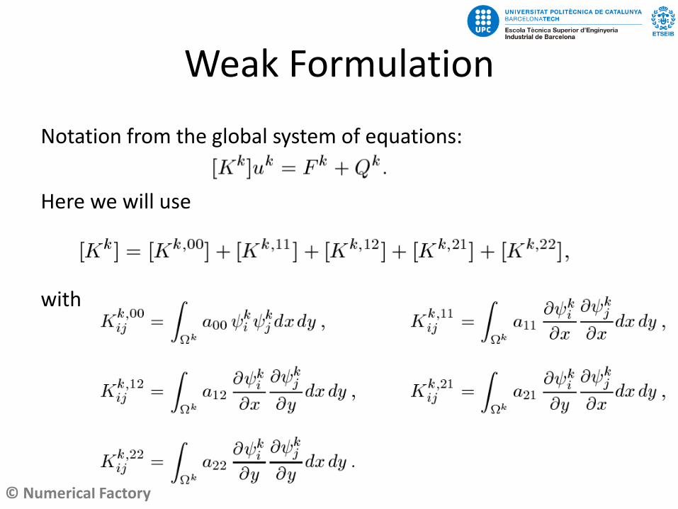
Notation from the global system of equations:
Here we will use
with
© Numerical Factory
Computing the Integrals
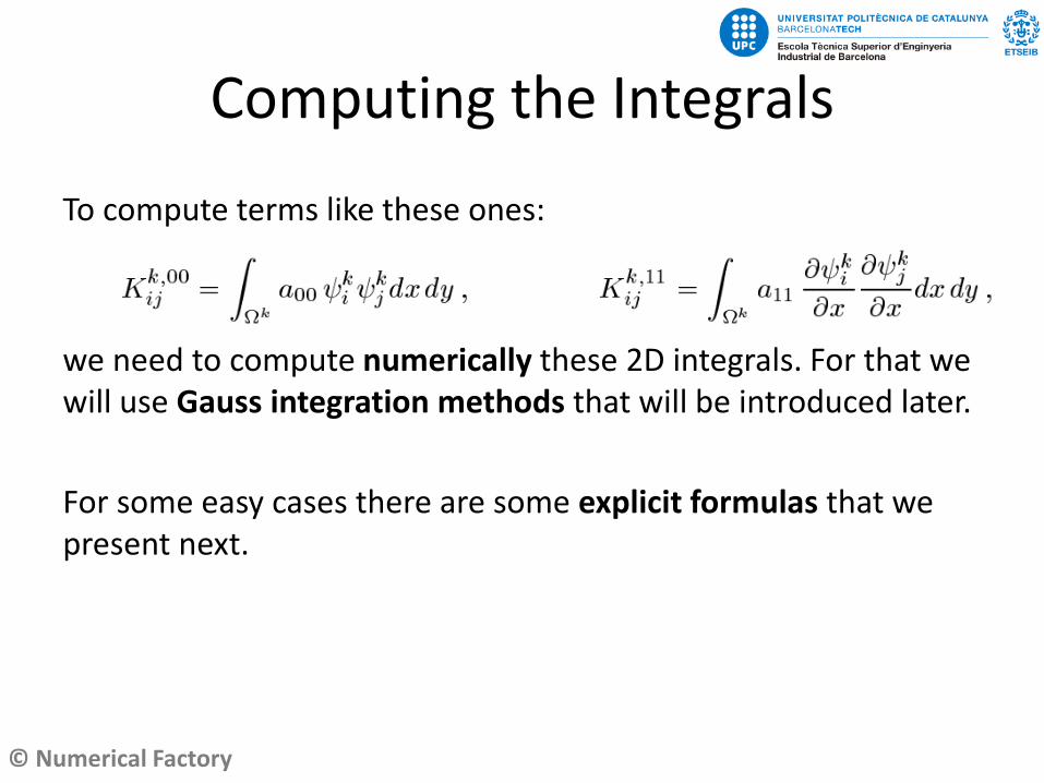
To compute terms like these ones:
we need to compute numerically these 2D integrals. For that we will use Gauss integration methods that will be introduced later.
For some easy cases there are some explicit formulas that we present next.
© Numerical Factory
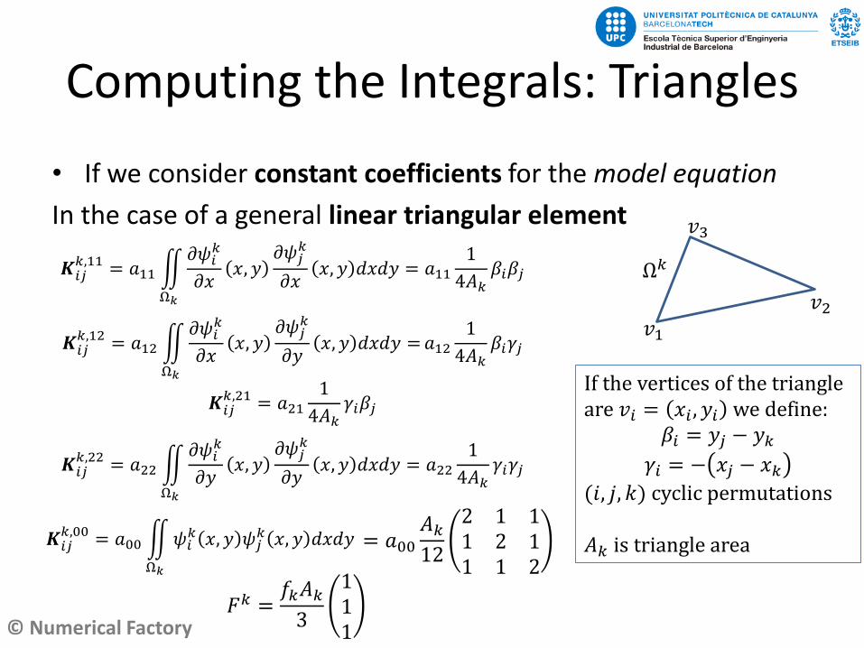
Computing the Integrals: Triangles
• If we consider constant coefficients for the model equation
In the case of a general linear triangular element
𝑲𝑖𝑗𝑘,11 = 𝑎11 ඵ
Ω𝑘
𝜕𝜓𝑖𝑘
𝜕𝑥𝑥, 𝑦
𝜕𝜓𝑗𝑘
𝜕𝑥𝑥, 𝑦 𝑑𝑥𝑑𝑦 = 𝑎11
1
4𝐴𝑘𝛽𝑖𝛽𝑗
𝑲𝑖𝑗𝑘,12 = 𝑎12 ඵ
Ω𝑘
𝜕𝜓𝑖𝑘
𝜕𝑥𝑥, 𝑦
𝜕𝜓𝑗𝑘
𝜕𝑦𝑥, 𝑦 𝑑𝑥𝑑𝑦 =𝑎12
1
4𝐴𝑘𝛽𝑖𝛾𝑗
𝑲𝑖𝑗𝑘,21 = 𝑎21
1
4𝐴𝑘𝛾𝑖𝛽𝑗
𝑲𝑖𝑗𝑘,22 = 𝑎22 ඵ
Ω𝑘
𝜕𝜓𝑖𝑘
𝜕𝑦𝑥, 𝑦
𝜕𝜓𝑗𝑘
𝜕𝑦𝑥, 𝑦 𝑑𝑥𝑑𝑦 = 𝑎22
1
4𝐴𝑘𝛾𝑖𝛾𝑗
𝑲𝑖𝑗𝑘,00 = 𝑎00 ඵ
Ω𝑘
𝜓𝑖𝑘 𝑥, 𝑦 𝜓𝑗
𝑘 𝑥, 𝑦 𝑑𝑥𝑑𝑦
If the vertices of the triangle are 𝑣𝑖 = 𝑥𝑖 , 𝑦𝑖 we define:
𝛽𝑖 = 𝑦𝑗 − 𝑦𝑘𝛾𝑖 = − 𝑥𝑗 − 𝑥𝑘
(𝑖, 𝑗, 𝑘) cyclic permutations
𝐴𝑘 is triangle area= 𝑎00𝐴𝑘12
2 1 11 2 11 1 2
𝐹𝑘 =𝑓𝑘𝐴𝑘3
111
𝑣1
𝑣2
𝑣3
Ω𝑘
© Numerical Factory
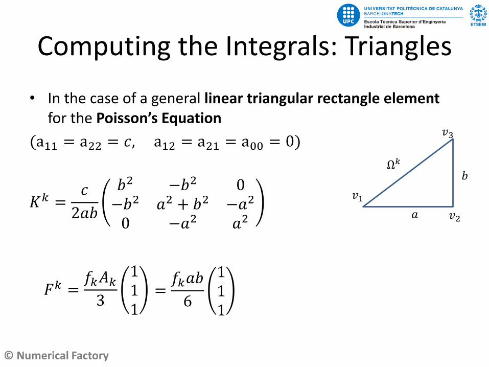
Computing the Integrals: Triangles
• In the case of a general linear triangular rectangle element for the Poisson’s Equation
(a11 = a22 = 𝑐, a12 = a21 = a00 = 0)
𝐾𝑘 =𝑐
2𝑎𝑏
𝑏2 −𝑏2 0−𝑏2 𝑎2 + 𝑏2 −𝑎2
0 −𝑎2 𝑎2
𝐹𝑘 =𝑓𝑘𝐴𝑘3
111
𝑣1
𝑣2
𝑣3
𝑎
𝑏Ω𝑘
=𝑓𝑘𝑎𝑏
6
111
© Numerical Factory
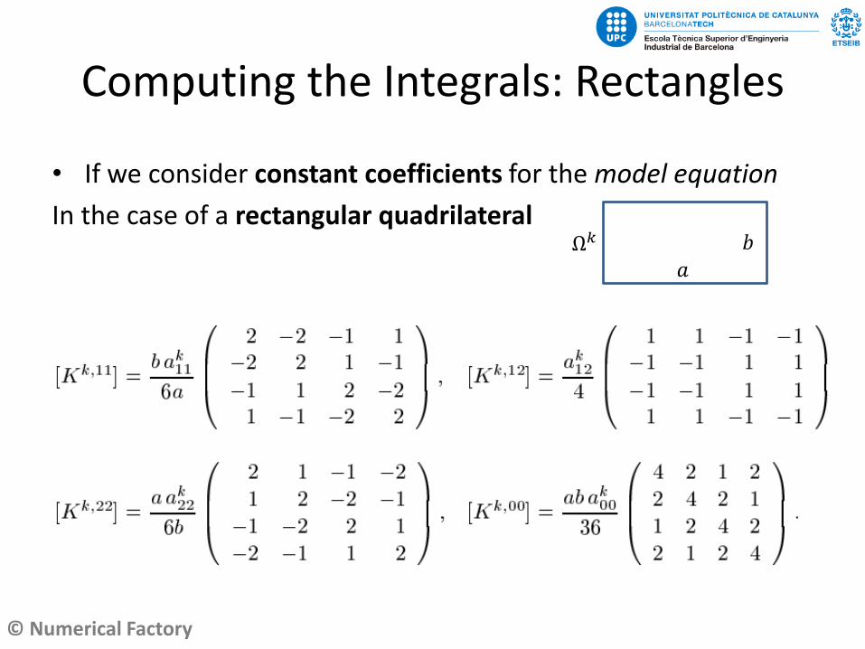
Computing the Integrals: Rectangles
• If we consider constant coefficients for the model equation
In the case of a rectangular quadrilateral
𝑎
𝑏Ω𝑘
© Numerical Factory
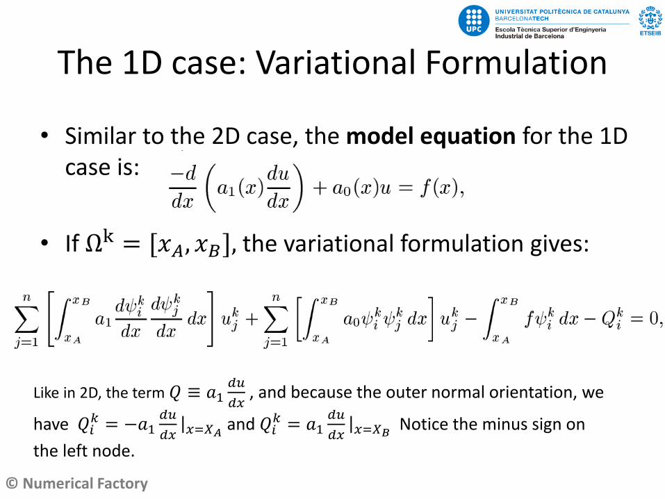
The 1D case: Variational Formulation
• Similar to the 2D case, the model equation for the 1D case is:
• If Ωk = [𝑥𝐴, 𝑥𝐵], the variational formulation gives:
Like in 2D, the term 𝑄 ≡ 𝑎1𝑑𝑢
𝑑𝑥, and because the outer normal orientation, we
have 𝑄𝑖𝑘 = −𝑎1
𝑑𝑢
𝑑𝑥ȁ𝑥=𝑋𝐴 and 𝑄𝑖
𝑘 = 𝑎1𝑑𝑢
𝑑𝑥ȁ𝑥=𝑋𝐵 Notice the minus sign on
the left node.
© Numerical Factory
The 1D case: Variational Formulation
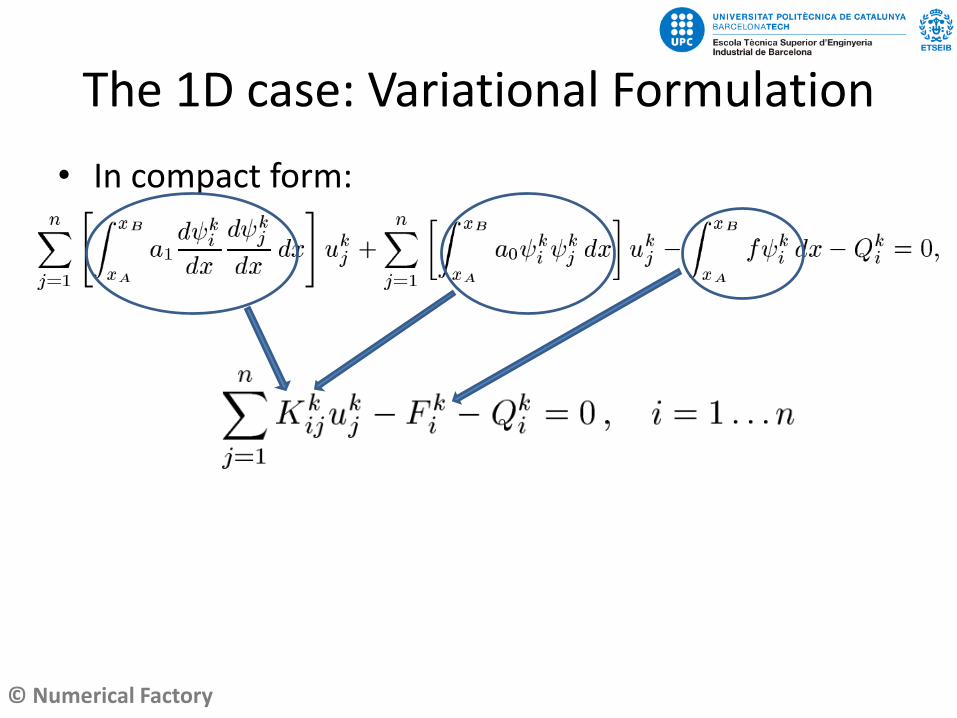
• In compact form:

© Numerical Factory
The 1D case: Variational Formulation
• In compact form:
Notice that now these are 1D integrals
© Numerical Factory
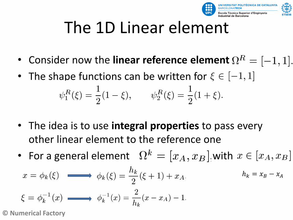
The 1D Linear element
• Consider now the linear reference element
• The shape functions can be written for
• The idea is to use integral properties to pass every other linear element to the reference one
• For a general element with
ℎ𝑘 = 𝑥𝐵 − 𝑥𝐴
© Numerical Factory
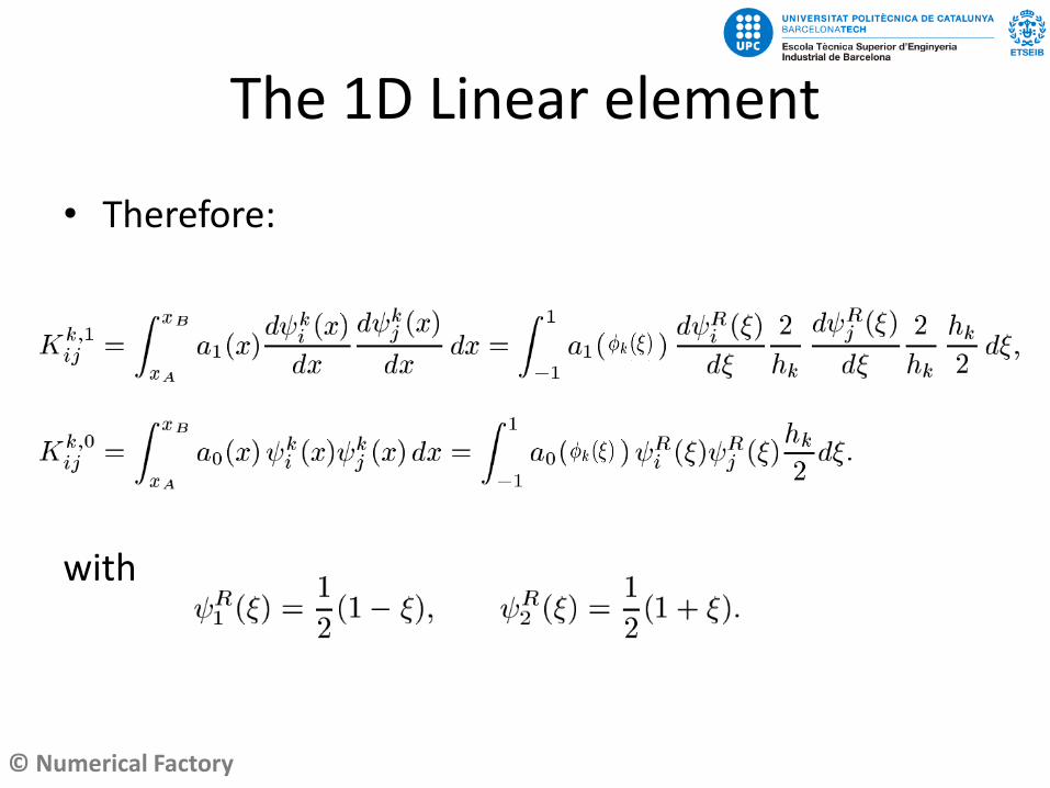
The 1D Linear element
• Therefore:
with
© Numerical Factory
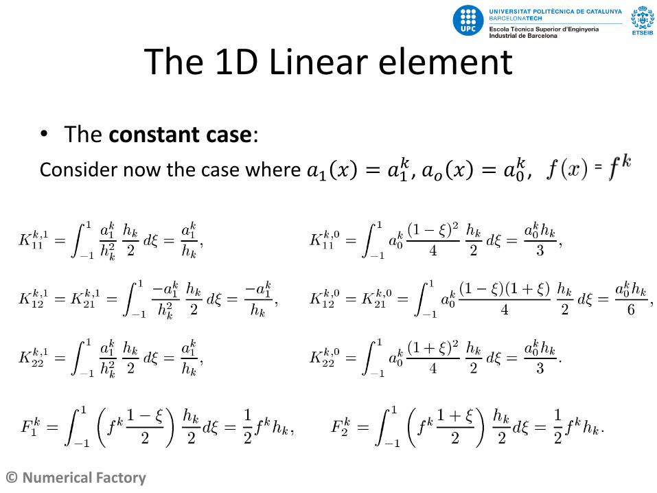
The 1D Linear element
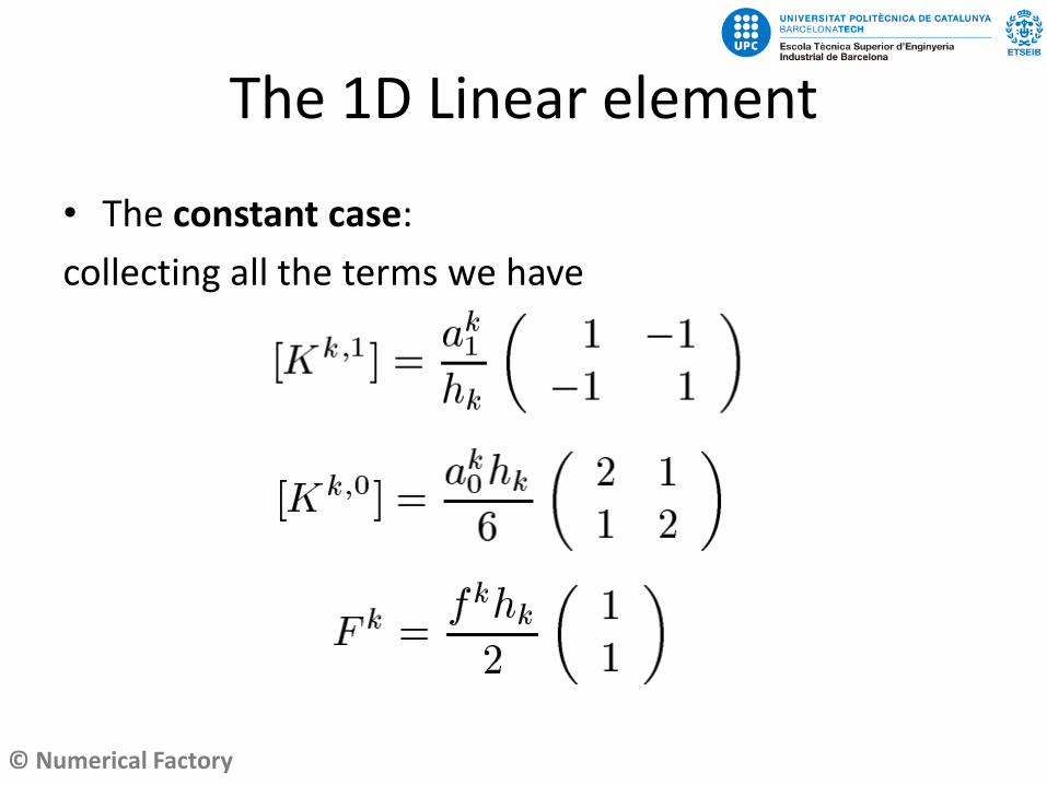
• The constant case:
Consider now the case where 𝑎1 𝑥 = 𝑎1𝑘, 𝑎𝑜 𝑥 = 𝑎0
𝑘, =
© Numerical Factory
The 1D Linear element
• The constant case:
collecting all the terms we have
© Numerical Factory
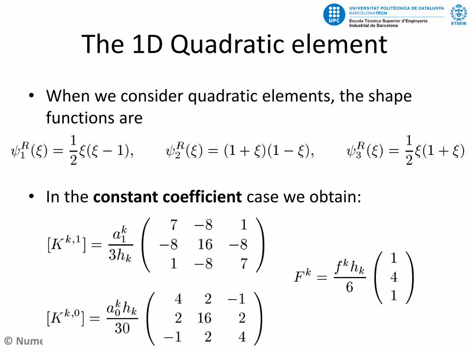
The 1D Quadratic element
• When we consider quadratic elements, the shape functions are
• In the constant coefficient case we obtain:
© Numerical Factory
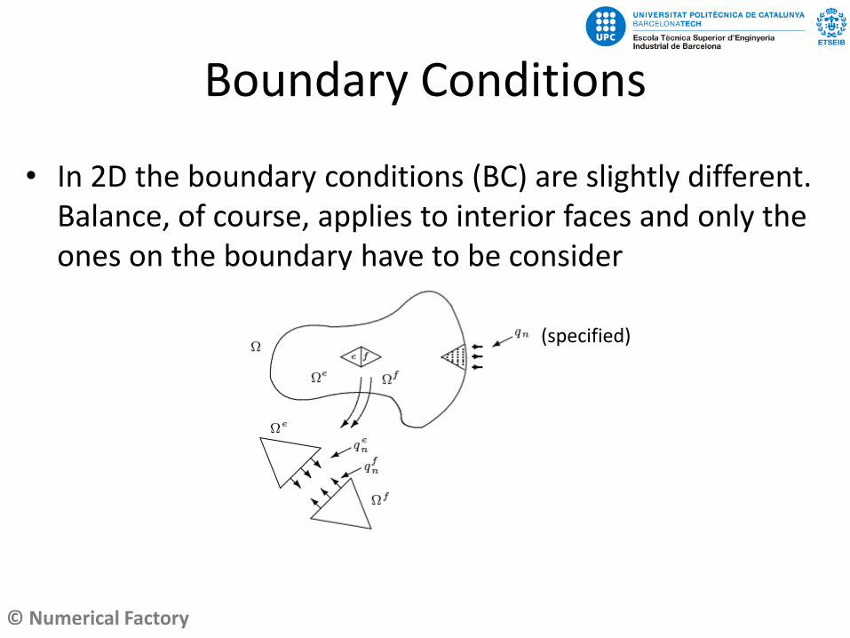
Boundary Conditions
• In 2D the boundary conditions (BC) are slightly different. Balance, of course, applies to interior faces and only the ones on the boundary have to be consider
(specified)
© Numerical Factory
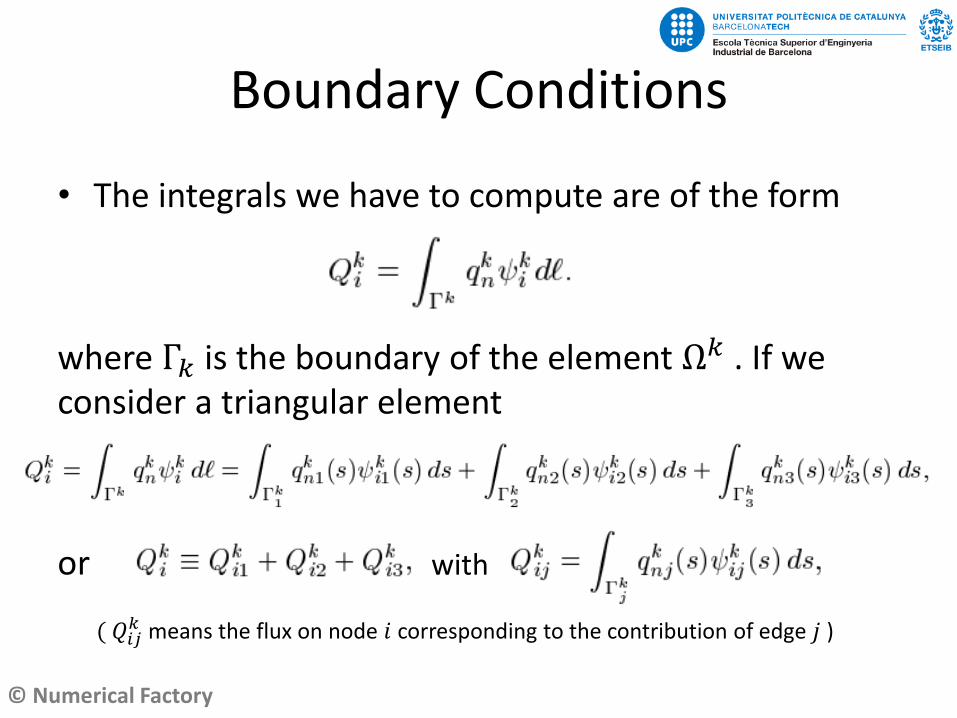
( 𝑄𝑖𝑗𝑘 means the flux on node 𝑖 corresponding to the contribution of edge 𝑗 )
Boundary Conditions
• The integrals we have to compute are of the form
where Γ𝑘 is the boundary of the element Ω𝑘 . If we consider a triangular element
or with
© Numerical Factory
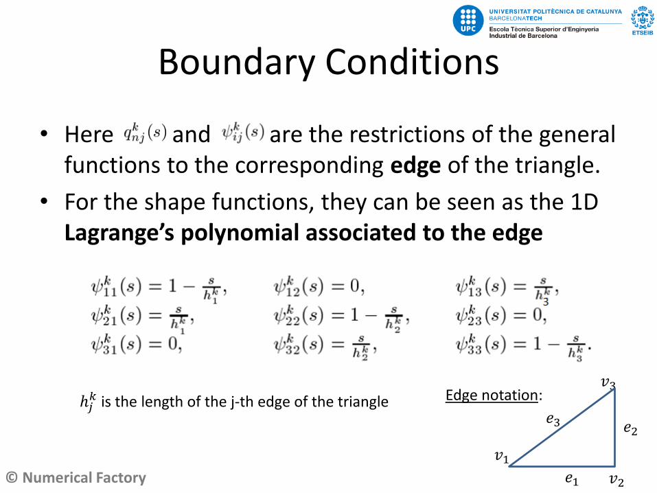
Boundary Conditions
• Here and are the restrictions of the general functions to the corresponding edge of the triangle.
• For the shape functions, they can be seen as the 1D Lagrange’s polynomial associated to the edge
ℎ𝑗𝑘 is the length of the j-th edge of the triangle
𝑣3
𝑣1𝑣2𝑒1
𝑒2𝑒3
Edge notation:
© Numerical Factory
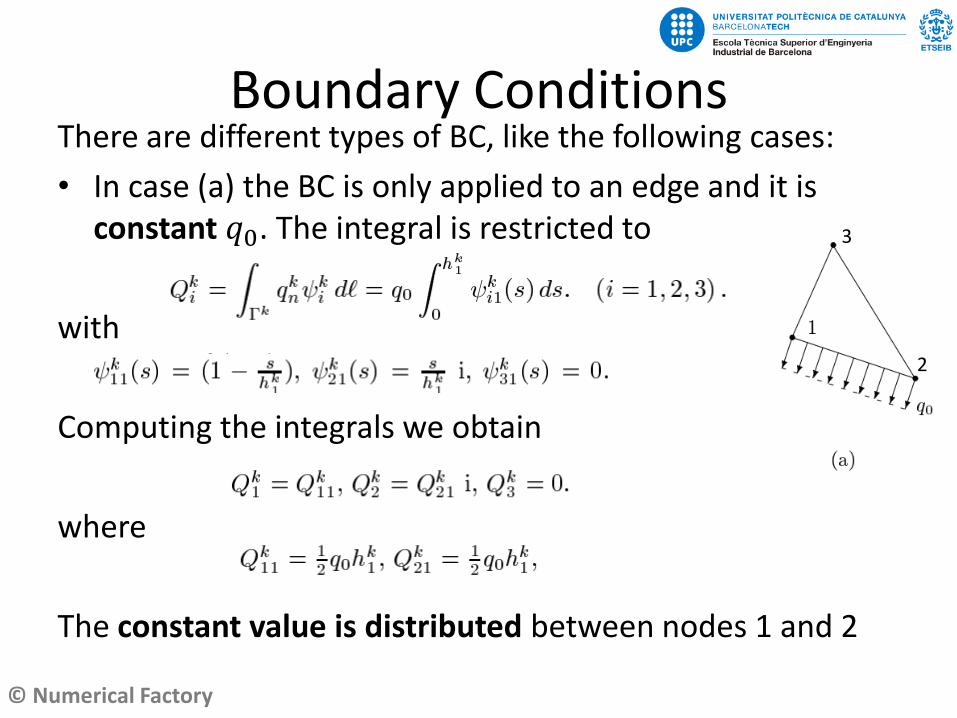
Boundary ConditionsThere are different types of BC, like the following cases:
• In case (a) the BC is only applied to an edge and it is constant 𝑞0. The integral is restricted to
with
Computing the integrals we obtain
where
The constant value is distributed between nodes 1 and 2
2
3
© Numerical Factory
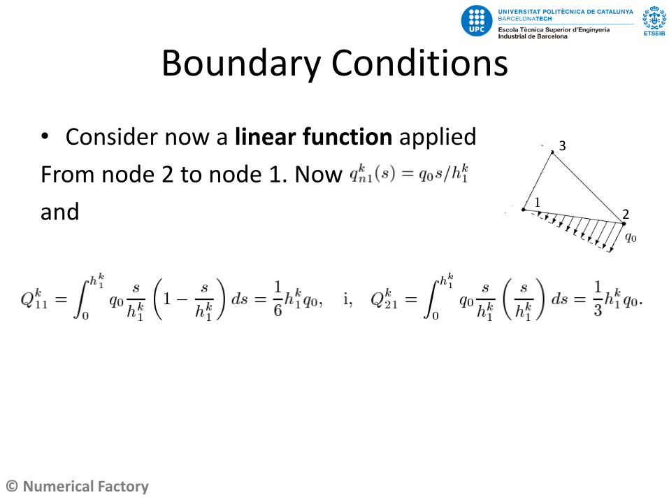
Boundary Conditions
• Consider now a linear function applied
From node 2 to node 1. Now
and 2
3
© Numerical Factory
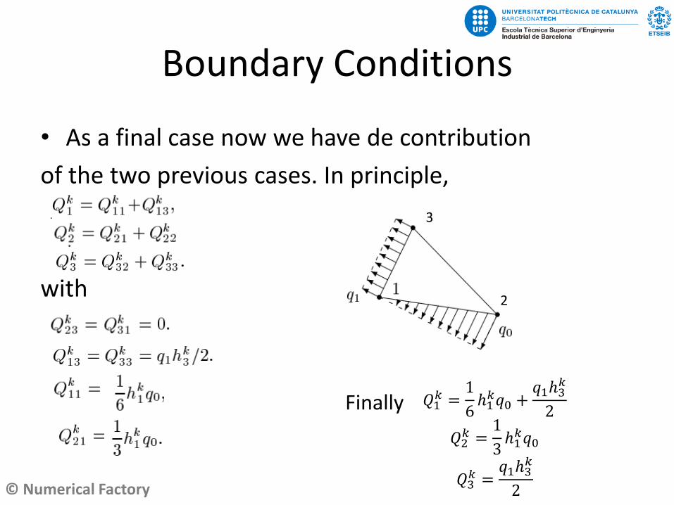
Boundary Conditions
• As a final case now we have de contribution
of the two previous cases. In principle,
with2
3
𝑄1𝑘 =
1
6ℎ1𝑘𝑞0 +
𝑞1ℎ3𝑘
2
𝑄2𝑘 =
1
3ℎ1𝑘𝑞0
𝑄3𝑘 =
𝑞1ℎ3𝑘
2
Finally
© Numerical Factory
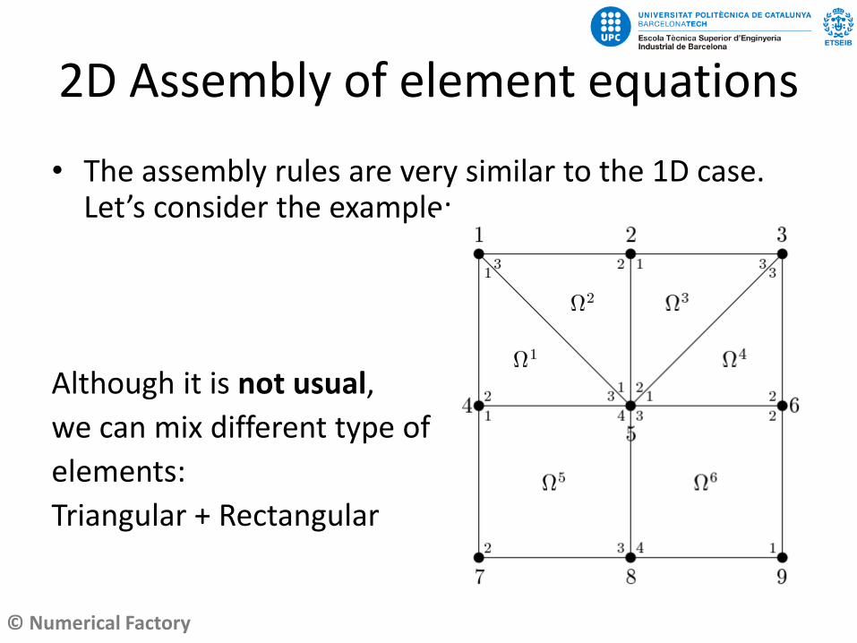
2D Assembly of element equations
• The assembly rules are very similar to the 1D case. Let’s consider the example:
Although it is not usual,
we can mix different type of
elements:
Triangular + Rectangular
© Numerical Factory
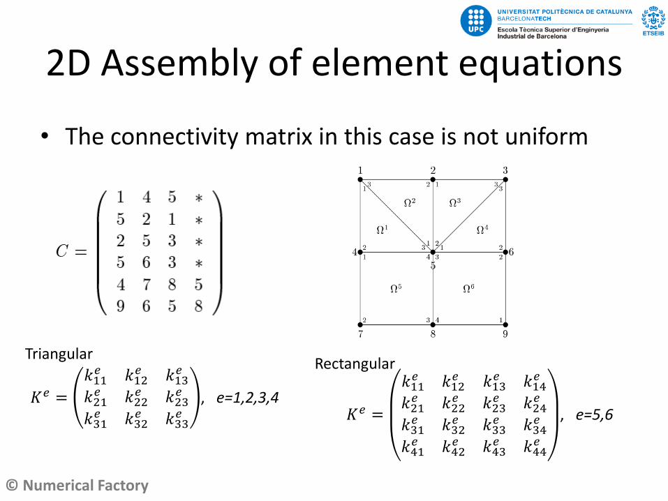
2D Assembly of element equations
• The connectivity matrix in this case is not uniform
𝐾𝑒 =
𝑘11𝑒 𝑘12
𝑒 𝑘13𝑒
𝑘21𝑒 𝑘22
𝑒 𝑘23𝑒
𝑘31𝑒 𝑘32
𝑒 𝑘33𝑒
, e=1,2,3,4𝐾𝑒 =
𝑘11𝑒 𝑘12
𝑒
𝑘21𝑒 𝑘22
𝑒𝑘13𝑒 𝑘14
𝑒
𝑘23𝑒 𝑘24
𝑒
𝑘31𝑒 𝑘32
𝑒
𝑘41𝑒 𝑘42
𝑒
𝑘33𝑒 𝑘34
𝑒
𝑘43𝑒 𝑘44
𝑒
, e=5,6
TriangularRectangular
© Numerical Factory
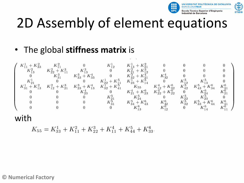
2D Assembly of element equations
• The global stiffness matrix is
with
© Numerical Factory
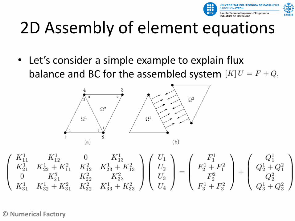
2D Assembly of element equations
• Let’s consider a simple example to explain flux balance and BC for the assembled system
2 2
© Numerical Factory
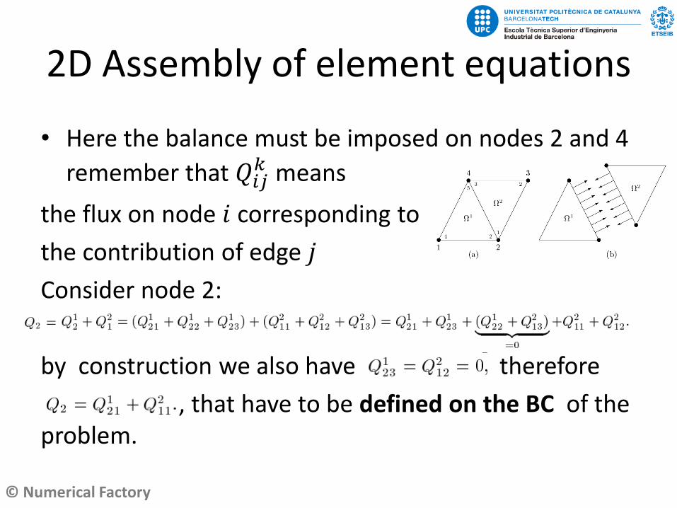
2D Assembly of element equations
• Here the balance must be imposed on nodes 2 and 4
remember that 𝑄𝑖𝑗𝑘 means
the flux on node 𝑖 corresponding to
the contribution of edge 𝑗
Consider node 2:
by construction we also have therefore
, that have to be defined on the BC of the problem.