Embed Size (px)
Citation preview

Covariance matrix estimation and variable selection in high dimension
by
Mu Cai
A dissertation submitted in partial satisfaction of the
requirements for the degree of
Doctor of Philosophy
in
Statistics
in the
Graduate Division
of the
University of California, Berkeley
Committee in charge:
Professor Peter J. Bickel , ChairProfessor Cari Kaufman
Professor Noureddine El KarouiProfessor James L. Powell
Spring 2013

Covariance matrix estimation and variable selection in high dimension
Copyright 2013by
Mu Cai

1
Abstract
Covariance matrix estimation and variable selection in high dimension
by
Mu Cai
Doctor of Philosophy in Statistics
University of California, Berkeley
Professor Peter J. Bickel , Chair
First part of the thesis focuses on sparse covariance matrices estimation under the sce-nario of large dimension p and small sample size n. In particular, we consider a class ofcovariance matrices which are approximately block diagonal under unknown permutations.We propose a block recovery estimator and show it achieves minimax optimal convergencerate for the class, which is the same as if the permutation were known. The problem isalso related to sparse PCA and k-densest subgraphs, where the spike model is a special caseof their intersection. Simulations of the spike model and multiple block model, togetherwith a real world application, confirm that the proposed estimator is both statistically andcomputationally efficient.
Second part of the thesis focuses on variable selection in linear regression, also underthe high dimensional scenario of large p and small n. We propose a general frameworkto search variables based on their covariance structures, with a specific variable selectionalgorithm called kForward which iteratively fits local/small linear models among relativelyhighly correlated variables. For simulation experiments and a real world data set, we comparekForward to other popular methods including the Lasso, ElasticNet, SCAD, MC+, FoBafor both variable selection and prediction.

i
Dedicated to my family and in memory of my grandmother Jia Zhen Yin.

CONTENTS ii
Contents
Contents ii
1 Notations 1
I High dimensional covariance matrix estimation 3
2 Introduction 42.1 Related Work . . . . . . . . . . . . . . . . . . . . . . . . . . . . . . . . . . . 5
3 Method 83.1 Problem Setup . . . . . . . . . . . . . . . . . . . . . . . . . . . . . . . . . . 83.2 Estimator . . . . . . . . . . . . . . . . . . . . . . . . . . . . . . . . . . . . . 93.3 Algorithm . . . . . . . . . . . . . . . . . . . . . . . . . . . . . . . . . . . . . 10
4 Analysis 144.1 Distributional Assumptions . . . . . . . . . . . . . . . . . . . . . . . . . . . 144.2 Optimal Support Recovery . . . . . . . . . . . . . . . . . . . . . . . . . . . . 154.3 Minimax Optimal Covariance Estimation . . . . . . . . . . . . . . . . . . . . 224.4 Algorithm Correctness and Computational Complexity . . . . . . . . . . . . 26
5 Experiment 345.1 Single Block Spike model . . . . . . . . . . . . . . . . . . . . . . . . . . . . . 345.2 Multiple Block Model . . . . . . . . . . . . . . . . . . . . . . . . . . . . . . . 395.3 Application . . . . . . . . . . . . . . . . . . . . . . . . . . . . . . . . . . . . 43
II High dimensional variable selection in linear model 47
6 Introduction 48
7 Method 527.1 General framework . . . . . . . . . . . . . . . . . . . . . . . . . . . . . . . . 52

CONTENTS iii
7.2 Algorithm . . . . . . . . . . . . . . . . . . . . . . . . . . . . . . . . . . . . . 54
8 Analysis 568.1 Support Recovery . . . . . . . . . . . . . . . . . . . . . . . . . . . . . . . . . 568.2 Special Block Model . . . . . . . . . . . . . . . . . . . . . . . . . . . . . . . 59
9 Experiment 619.1 Simulation . . . . . . . . . . . . . . . . . . . . . . . . . . . . . . . . . . . . . 619.2 Application . . . . . . . . . . . . . . . . . . . . . . . . . . . . . . . . . . . . 63
10 Minimal Context 717110.2 Algorithm . . . . . . . . . . . . . . . . . . . . . . . . . . . . . . . . . . . . . 7610.3 Simulation . . . . . . . . . . . . . . . . . . . . . . . . . . . . . . . . . . . . . 77
Bibliography 81

CONTENTS iv
Acknowledgments
It is a great pleasure to thank the many people who made this thesis possible. First andforemost I would like to thank my advisor Professor Peter Bickel. I am extremely gratefulto Peter for his continuous support, guidance and insightful advice throughout the years. Iam also very thankful to my committee, Professor Cari Kaufman, Professor Noureddine ElKaroui and Professor James Powell, for their kind assistance and advice for my qualificationexam and my thesis. I want to thank Professor Boaz Nadler from Weizmann Institute ofScience and Professor Ya’acov Ritov from The Hebrew University for sharing interestingideas and examples with me, many of which lead to the very foundation of my thesis. Ialso thank Dr. Aiyou Chen from Google for all the fruitful discussions which in manyways inspired this thesis. I am indebted to my colleagues Jingyi Jessica Li, Rachel Wangand Nathan Boley for sharing valuable data and application with me. I am grateful toProfessor Jim Pitman, Professor Terry Speed, Professor Bin Yu, Professor Haiyan Huang,Dr. Choongsoon Bae, Dr. Sheng Ma, Professor Ching-Shui Cheng, Professor Yun Song,Ryan Lovett, La Shana Porlaris, Denise Yee, Judith Foster and many others for their kindadvice and help. I also want to thank my undergraduate mentor Professor Almut Burchard,Professor Charles Pugh, Professor Steve Tanny and Professor Balint Virag from Universityof Toronto. At last, I thank my family and all my friends, especially my parents Chong BangCai and Qiang Li and my fiance Yi Ru Qin, for their endless support and encouragement.

CHAPTER 1. NOTATIONS 1
Chapter 1
Notations
• Define [n] = 1, 2, ..., n.
• For L = l1, l2, ..., ln, denote Li = li for i = 1, ..., n.
• Denote In×n the n by n identity matrix.
• Denote S+p the set of p× p positive definite matrices.
• Denote Πp the set of all permutations of [p].
• For vector v ∈ Rn,
– lq norm for q ≥ 1: ‖v‖q = (∑n
i=1 |vi|q)1q
– l0 norm: ‖v‖0 =∑n
i=1 I(vi 6= 0)
– l∞ norm: ‖v‖∞ = maxni=1 |vi|– v = 1
n
∑ni=1 vi
– vL = (vi)i∈L ∈ R|L| for ∀L ⊂ [n]
– The support of v: supp(v) = i : I(vi 6= 0)
• For matrix A ∈ Rn×p, vector v ∈ Rn,
– λmax(A): largest eigenvalue of A
– λmin(A): minimal eigenvalue of A
– lq operator norm for q ≥ 1: ‖A‖q = maxv 6=0‖Av‖q‖v‖q
– Spectral norm for square A with n = p: ‖A‖ = ‖A‖2 =√λmax(AtA)
– l1 norm: ‖A‖1 = max1≤j≤p∑n
i=1 |Aij|– l∞ norm: ‖A‖∞ = max1≤i≤n
∑pj=1 |Aij|

CHAPTER 1. NOTATIONS 2
– Frobenius norm: ‖A‖F =√∑n
i=1
∑pj=1 |Aij|2
– Aj ∈ Rn×1 is the jth column of A
– A(i) ∈ R1×p is the ith row of A
– For i0 ∈ [n], j0 ∈ [p], L ⊂ [n], J ⊂ [p], B ⊂ [p]× [p],
∗ AL,J = (Aij)i∈L,j∈J ∈ R|L|×|J |
∗ AJ = (Aij)1≤i≤n,j∈J ∈ Rn×|J |
∗ A(L) = (Aij)i∈L,1≤j≤p ∈ R|L|×p
∗ Ai0J = (Ai0j)j∈J ∈ R1×|J |
∗ ALj0 = (Aij0)i∈L ∈ R|L|×1
∗ AB = (AijI((i, j) ∈ B))1≤i,j≤p
∗ vtABv =∑p
(i,j)∈B vivjAij
– A = (Aj)1≤j≤p ∈ R1×p.

CHAPTER 1. NOTATIONS 3
Part I
High dimensional covariance matrixestimation

CHAPTER 2. INTRODUCTION 4
Chapter 2
Introduction
Covariance estimation plays a central role in many statistical methodologies including re-gression analysis, principal component analysis (PCA), linear and quadratic discriminantanalysis (LDA, QDA). Suppose X ∈ Rn×p is observed. The rows X(1), ..., X(n) ∈ R1×p
are i.i.d. p-variate random variables with covariance matrix Σ = (Σij)1≤i,j≤p. The goalis to construct an estimator Σ that is close to the population Σ. There are many met-rics for measurements. For example element-wise estimation corresponds to minimizingmaxi,j |Σij − Σij|, while techniques like PCA and LDA require estimation of eigenvalues,eigenvectors of Σ, and measurement of Σ− Σ with errors measured by the Frobenius norm‖.‖F or spectral norm ‖.‖. A classical approach is to estimate Σ by the empirical covari-ance matrix Σ = 1
n−1
∑ni=1(X(i)− X)T (X(i)− X). Nowadays many applications involve high
dimensional data with p > n or p = O(n). This poses many new challenges to classicalstatistics and extensive research has been done in this area. As an example, although Σ still
performs well for element-wise estimation with a convergence rate of√
1n, it is well known it
does not work for estimation of eigenvalues, eigenvectors for matrices Σ such as the identity,which are of high rank, and not approximable in the spectral norm by matrices of boundedrank.
However following work by various authors, Bickel and Levina (BL2008a-1) (BL2008b-1),T. Cai et al (CZZ2010-1) (CZ2012-1) , El Karoui (EK2007-1), it has been shown that if popu-lation matrices can be approximated in the spectral norm by structured matrices with sparsestructure, then estimates of these matrices converging at reasonable rates can be construct-ed even if p > n. Such matrices arise naturally if there is a metric on the variables suchthat high distance between the variables is associated with local covariance. For instance, ifX(1) = (X1t1 , ..., X1tp), where the tj correspond to times in a given year, such a metric is theusual Euclidean metric ρ(X1ta , X1tb) = |ta− tb|. More complicated structures can arise fromspatial fields. The natural approximation here are Σ of the form:
Σ(δ) = ΣijI(ρ(X1i, X1j) ≤ δ) (2.1)
Another possibility, see Furrer and Bengtsson (FB2007-1), is to replace the indicators by a

CHAPTER 2. INTRODUCTION 5
monotone tapering function σ(ρ(X1ta , X1tb)) which is monotone decreasing to 0 and
(σ(ρ(X1ta , X1tb)))1≤a,b≤p
is a positive definite matrix.In examples such as we have given above, the metric is known and the approximating
matrices can be readily constructed. However suppose there is a reason to believe that ametric of this type is present but not known in advance. For instance, suppose the variablesare expression of genes in a biochemical pathway. The metric which is unknown, is roughlygeodesic distance in the graph representing the pathway. We are then faced with approxi-mating a given covariance matrix by a matrix which, after an unknown permutation of thevariables, is of the given structure. That is the topic of the first part of the thesis.
We note that similar problems in which we assume that the approximating class hasrestrictions only on the member of zeros of the matrix, but not their position have beentreated. El Karoui (EK2007-1) proposed and analyzed a class of covariance matrices with β-sparsity, which requires the number of walks of length k on the graph with adjacency matrixinduced by the population covariance matrix is bounded by O(pβ(k−1)+1). He proposed anentry-wise thresholding estimator and showed that it is consistent in operator norm. Bickeland Levina (BL2008a-1) (BL2008b-1) proposed and analyzed approximately bandable classand classes with lq ball constraint on each row. They also provided upper bound on spectralnorm for corresponding thresholding and banding estimator. Another focus has been onapproximating covariance matrices for particular purpose such as PCA, CCA, some of whichassume structured sparse approximation, Amini and Wainwright (AW2009-1), Johnstone(J2001-1), and others does not, d’Aspermont et al(DA2007-1), Zou, Hastie and Tibshirani(ZHT2006-1), Joliffe et al (J2003-1). Another direction involves estimation of Σ−1. Forstructured situations, the results of Bickel and Lindner (BL2010-1) suggest quite generallythat inverting estimates of Σ taking advantage of the assumed structure works as well aspossible. Also Bickel and Levina (BL2008a-1) (BL2008b-1) give methods for estimating Σ−1
directly in structurally approximable cases, and see graphical Lasso Friedman, Hastie andTibshirani (FHT2008-1), Rothman et al (R2008-1) for unstructured sparse cases. We beginby reviewing some of this work.
2.1 Related Work
Following Bickel and Levina (BL2008a-1) (BL2008b-1), define classes of lq sparse covariancematrices as:
Ut(q, k0,M0) = Σ : Σii < M0,
p∑j=1
|Σij|q ≤ k0, for ∀i (2.2)
The classes of approximately bandable covariance matrices is defined as:
Ub(α,C,M) = Σ : maxj
∑i
|Σij| : |i− j| > k ≤ Ck−α, λmax(Σ) < M (2.3)

CHAPTER 2. INTRODUCTION 6
Define thresholding estimator:
Th(Σ) = (ΣijI(|Σij| > h))1≤i,j≤p (2.4)
Define banded estimator:
Bk(Σ) = (ΣijI(|i− j| ≤ k))1≤i,j≤p (2.5)
In a series of work by T. Cai et al (CZZ2010-1) (CL2011-1) (CY2012-1) (CZ2012-1) , minimaxconvergence rates in various norms and adaptive estimators were developed for similar classesof sparse covariance matrices. Their main results showed
infΣ
supΣ∈Ut(q,k0,M0)
E‖Σ− Σ‖2 k20(
log p
n)1−q (2.6)
and
infΣ
supΣ∈Ub(α,C,M)
E‖Σ− Σ‖2 n−2α
2α+1 +log p
n(2.7)
The thresholding estimator Th(Σ) with threshold h = O(√
log pn
) achieves the optimal con-
vergence rate for class Ut(q, k0,M0), and banded estimator Bk(Σ) with bandwidth k =O(n1/(2α+1)) achieves optimal convergence rate for class Ub(α,C,M). Both estimators canbe made adaptable.
Results from T. Cai et al (CZZ2010-1) (CZ2012-1) showed convergence rates of approx-imately bandable classes are in general faster than the rates of classes with lq constraintson rows. To do this, they showed that the banded estimator would behave as the empiricalestimator for small blocks with size equivalent to the bandwidth. This suggests a naturalquestion: suppose the population covariance matrix is not originally bandable, however un-der certain unknown permutation of its indices, it could be permuted into a approximatelybandable structure, is it possible to obtain the same convergence rate as if the permutationwere known? The answer is yes for some classes. We are particularly interested in thoseapproximately block diagonal after permutation. Denote the class in consideration as F .Our goal is to construct and analyze an estimator Σ∗ with spectral norm convergence rateminimax optimal:
supΣ∈F
E‖Σ∗ − Σ‖2 infΣ
supΣ∈F
E‖Σ− Σ‖2 (2.8)
The idea is to recover the unknown permutation to construct approximately block diagonalempirical covariance matrices. Then as with banding, we will show estimates keeping entrieswithin blocks and ignoring others would achieve the optimal rates.
The problem, as we pose it, is to recover unknown blocks of variables with relatively highercorrelations among themselves than outside. There are several closely related problems thathave been extensively studied in the literatures. For example, sparse PCA considers thefollowing NP hard problem
v = arg max‖v‖0≤k, ‖v‖=1
vtΣv (2.9)

CHAPTER 2. INTRODUCTION 7
The goal is to estimate the first principal component (eigenvector of Σ corresponding tolargest eigenvalue) under the assumption that the eigenvector has at most k nonzero en-tries. Using the Lasso by Tibshirani (T1996-1), Jolliffe et al (J2003-1) proposed SCoTLassalgorithm which replaces the constraint on l0 norm by l1 norm. Zou, Hastie and Tibshirani(ZHT2006-1) proposed the SPCA algorithm which derives sparse principal components bysolving self-constrained regression regularized by l1 norm. d’Aspremont et al (DA2007-1)proposed the DSPCA algorithm which relaxes the l0 constraint and transform the originalproblem to a semi-definite program(SDP):
V = arg maxV0, tr(V )=1
tr(ΣV )− ρn∑i,j
|Vij| (2.10)
Amini and Wainwright (AW2009-1) analyzed the statistical properties of this method overa class of spike models
Eβ = Σ : Σ = βzzt +
[Ik×k 0
0 Γp−k
], λmax(Γp−k) ≤ 1, zi = ± 1√
k (2.11)
They showed that, under some mild assumptions, and if the solution of 2.10 is rank 1, then itagrees with the solution of the exact problem and achieves the global optima. Furthermore,if the sample size n = ck log p for sufficiently large constant c, block can be recoveredwith probability going to 1 for any block size k ≥ c′ log p. However, as we have shownin simulation, the essential existence of rank 1 solution is usually not satisfied, and theSDP approach is not rate optimal. Xiaotong Yuan and Tong Zhang (YZ2011-1) proposeda truncated power method called TPower and analyzed its property with more generalassumptions on covariance matrices. Their method is very similar to our algorithm FBand FBRec defined in Chapter 3, except that we do not re-weight the solution and we usedifferent input matrix other than using the empirical covariance matrix directly. As thegoals and analysis are quite different, our results are not directly comparable. Their goalis to recover largest sparse eigenvector and the analysis requires conditions on eigen-gapbetween the largest and second largest eigenvalue. We consider a different multiple blockmodel and do not require any eigen-gap or rank conditions.
In Chapter 3, we formally setup the problem and define the appropriate class of co-variance matrices, then propose corresponding estimator and algorithms. Our main re-sults are in Chapter 4, where we analyze the statistical and computational properties ofthe proposed estimator and algorithms. We show that under some regularity conditions,if k = O(log p), n ≥ O(k2), and most entries within blocks have signal strength at least
O( 1√n), which is weaker comparing to O(
√log pn
) signal strength required by thresholding,
then our algorithm is rate optimal for support recovery, and the induced estimator achievesminimax optimal convergence rate in spectral norm. We also upper bound the worst casecomputational complexity of the algorithm with high probability. In Chapter 5, we showby simulations of the spike model and multiple block model to confirm that the proposedestimator is both statistically and computationally efficient.

CHAPTER 3. METHOD 8
Chapter 3
Method
3.1 Problem Setup
Recall that we are particularly interested in a class, denote as F , of covariance matricesapproximately block diagonal after unknown permutation. Our goal is to construct andanalyze an estimator Σ∗ with spectral norm convergence rate minimax optimal:
supΣ∈F
E‖Σ∗ − Σ‖2 infΣ
supΣ∈F
E‖Σ− Σ‖2 (3.1)
The idea is to recover the unknown permutation to construct approximately block diagonalempirical covariance matrices. Then as with banding, we will show estimates keeping entrieswithin blocks and ignoring others would achieve the optimal rates.
Next we define exactly the class F of covariance matrices approximately block diagonalafter unknown permutation. Denote the set of indices as [p] = 1, 2, ..., p. A block B is aset of pair indices if ∃J ⊂ [p] s.t. B = J × J = (i, j) : i, j ∈ J. Define the support ofany set of pair indices B as J(B) = i : ∃j s.t. (i, j) ∈ B or (j, i) ∈ B. Let I(.) denote theindicator function. B is an approximate block if B ∈ B(k,M, ε) :
B(k,M, ε) = B : Mk ≥ |J(B)| ≥ k,∑j∈J(B)
I((i, j) 6∈ B) ≤ εk for ∀i ∈ J(B) (3.2)
k is the order of sizes of blocks and will grow with dimension p. M and ε are parameters andconsidered constants. ε is a measurement of proximity of B to a block. If ε is close to 0, thenmost (i, j) ∈ J(B)× J(B) are in B, and B is close to a block. M is a constraint so that allblocks are at the same order. A set of approximate blocks Blml=1 are approximately blockdiagonal if Blml=1 ∈ B(k,M, ε, δ) :
B(k,M, ε, δ) = Blml=1 : Bl ∈ B(k,M, ε), |J(Bl) ∩ (∪i 6=lJ(Bi))| ≤ δk (3.3)
∃ partition L1 t L2 = [m] s.t. Bi ∩Bj = ∅ for ∀(i, j) ∈ (L1 × L1) ∪ (L2 × L2) (3.4)

CHAPTER 3. METHOD 9
where δ is similar to ε and is a measurement of overlaps among blocks. If δ is close to 0,then the blocks have little overlap and are close to block diagonal. The condition
∃ partition L1 t L2 = [m] s.t. Bi ∩Bj = ∅ for ∀(i, j) ∈ (L1 × L1) ∪ (L2 × L2)
could be relaxed to that ∃ constant q uniformly for all (n, p, k) in consideration,
∃ partition tqi=1 Li = [m] s.t. Bi ∩Bj = ∅ for ∀(i, j) ∈ ∪qi=1(Li × Li)
This condition is to regularize the way blocks intersecting each other, for example, it excludescounter example proposed by El Karoui (EK2007-1) that Σ being diagonal with all othernon-zero entries 1√
ponly in the first row and the first column. We will describe how the
ranges of M , ε and δ affect the estimator in Chapter 4. Recall that S+p is the set of p × p
positive definite matrices, and Πp is the set of all permutations of [p]. The class of covariancematrices we are interested in is defined as follows:
F(λ, k,m,M, ε, δ) = Σ ∈ S+p : ∃π ∈ Πp,∃Blml=1 ∈ B(k,M, ε, δ) (3.5)
s.t. Σπ(i)π(j) = aijI((i, j) ∈ ∪ml=1Bl) with |aij| > λ for i 6= j,Σii = 1 (3.6)
It requires that under unknown permutation π, Σ can be permuted to approximately blockdiagonal with small overlaps among the blocks, and most entries within blocks are of signalstrength at least λ. WLOG, we also assume Σii = 1 for all i. Recall our goal is to constructan estimator Σ∗ with minimax optimal convergence rate in spectral norm:
supΣ∈F(λ,m,k,M,ε,δ)
E‖Σ∗ − Σ‖2 infΣ
supΣ∈F(λ,m,k,M,ε,δ)
E‖Σ− Σ‖2 (3.7)
The key parameter is the signal strength λ, since the larger λ the easier the problem. An
extreme case would be λ = O(√
log pn
). In this case if λ = c√
log pn
with a large enough
constant c, the thresholding estimator Th(Σ) with threshold h = O(√
log pn
), see El Karoui
(EK2007-1), Bickel and Levina (BL2008a-1)(BL2008b-1), achieves the optimal convergencerate. Our main result pushes to λ = O( 1√
n) but for more specific classes with underlying
block structures.
3.2 Estimator
In this section we construct a block recovery estimator with corresponding algorithms. In-spired by the analysis of banding, see T. Cai et al (CZZ2010-1), one way to estimate ap-proximately block diagonal Σ at fastest rate would be keeping empirical estimates inside theblocks and ignore the remaining entries. Specifically, our estimator Σ∗ of Σ is constructedas follows:
Σ∗ij = ΣijI((i, j) ∈ ∪ml=1Bl) with Bl = Jl × Jl (3.8)

CHAPTER 3. METHOD 10
where Σ is the the empirical covariance matrix, and Jlml=1 are our estimate for the supportof the blocks. Since permutation π is unknown, the main difficulty is to construct goodestimates Jl of Jl for short of J(Bl). Note that the estimator is invariant under any particularlabeling as long as Blml=1 = Jl × Jlml=1. We construct estimates for supports for l =1, 2, ...,m recursively,
J(Bl) = Jl(θ1, θ2, t) = arg maxJ|J | ≥ k :
1
|J |∑j∈J
I(|Σij| < t) ≤ θ1 for ∀i ∈ J, |J∩(∪l−1i=1Ji)| ≤ θ2k
(3.9)where θ1, θ2, t are input parameters and their values depend on λ and max(ε, δ). The choicesof θ1, θ2, t depend on k and λ, and the specific form is given in Theorem 4.2.1.
The main issue for support recovery is computational cost. One may recognize that itlooks similar to the hidden-clique recovery problem and k-densest subgraph problem, whichare NP-hard in general. Indeed, consider the graph G(V , E) induced by empirical covariancematrix with vertices V = [p] and edges E = (i, j) : |Σij| > h for some threshold h. DenoteEh the corresponding adjacency matrix:
Eh = (I((i, j) ∈ E))1≤i,j≤p = (I(|Σij| > h))1≤i,j≤p (3.10)
As will be shown later, then support recovery problem (3.9) for a single block is equivalentto
J1 = arg maxJ :|J |=|J(B1)|
∑i,j∈J
(Eh)ij (3.11)
In general, if E is adjacency matrix of an arbitrary graph, this is the densest k subgraph prob-lem and computationally intractable. However, G here is induced by thresholding empiricalcovariance matrix and not completely arbitrary.
3.3 Algorithm
For given threshold h, consider two matrices as potential inputs for algorithms:
Eh = (I(|Σij| > h))1≤i,j≤p (3.12)
andWh = (|Σij|I(|Σij > h| and i 6= j))1≤i,j≤p (3.13)
Let A denote the generic input matrix. Our main results in Chapter 4 are based on inputA = Eh. However, as shown in simulated experiments in Chapter 5, input A = Wh isbetter in simulation. Specifically, algorithm FBRec is proposed to recover a single block,and FBAll recovers multiple blocks by repeatedly applying FBRec. The pseudo code is asfollows:

CHAPTER 3. METHOD 11
FB(A, J, k, t)
p← dimension of Afor i = 1 to t doRl ←
∑j∈J Ajl for l = 1, ..., p
J ′ ← indices of the top k largest elements of Rlpl=1
if J == J ′ thenbreak
elseJ ← J ′
end ifend forreturn J
FBS(A, J, θb, θr, t)
J ′ ← FB(A, J, |J |+ 1, t)while mini∈J ′
1|J ′|∑
j∈J ′ Aij > θr and 1|J ′|2
∑i,j∈J ′ Aij > θb do
J ← J ′
J ′ ← FB(A, J, |J |+ 1, t)end whilereturn J
FBRec(A,L, J, k, s, θb, θr, t)
if s > 0 thenfor l = 1 to |L| do
(J0, L′, b)← FBRec(A, j ∈ L : ALlj 6= 0, J ∪ Ll, k, s− 1, θb, θr, t)
if b > θb and mini∈J01|J0|∑
j∈J0 Aij > θr and |J0| ≥ k thenBREAK
end ifend for
elseb← 0for l = 1 to |L| doJ ′ ← FB(A,Ll ∪ J, k, t)if 1|J ′|2
∑i,j∈J ′ Aij > b then
b← 1|J ′|2
∑i,j∈J ′ Aij
J0 ← J ′
if b > θb and mini∈J01|J0|∑
j∈J0 Aij > θr then
J0 ← FBS(A, J0, θb, θr, t)break
end if

CHAPTER 3. METHOD 12
end ifend for
end ifL← Ljj>lreturn (J0, L, b)
Remark: For more efficient computation, the above step
J ′ ← FB(A,Ll ∪ J, k, t)could be replaced by:
J ′ ← FB(AL∪J,L∪J , Ll ∪ J, θ|J |r k, t)
The proof of algorithm correctness with this replacement would follow from the proof of The-orem 4.4.1 but more technical. For simplicity, Theorem 4.4.1 proves algorithm correctnesswithout this replacement.
FBAll(A, k, s, θb, θr, t)
p← dimension of AL← [p]l← 0while |L| ≥ k do
(J0, L, b)← FBRec(A,L, ∅, k, s, θb, θr, t)if b > θb and mini∈J0
1|J0|∑
j∈J0 Aij > θr and J0 6∈ Bjlj=1 thenl← l + 1Bl ← J0
L← L\J0
end ifend while
The idea for FBRec(A, [p], ∅, k, s, θb, θr, t) is to exhaustively search over all |J | = s + 1satisfying
Aij 6= 0 for ∀i, j ∈ J (3.14)
and FB(A, J, k, t) is called for each such J . As shown in Theorem 4.4.1, in order for FBRec()to success with high probability, s = ηk is required with η > 0 uniformly, i.e. s = O(k).When s = 0, FBRec() is very similar to TPower by X.T. Yuan and T. Zhang (YZ2011-1)with special initialization for the spike model in 2.11. FB() iteratively updates J by top klargest row sum Rl over J . As it does not necessarily converge, t upper bounds the numberof iterations. As we will show in Theorem 4.4.1, if start with J a subset of some block Jland |J | = s + 1 is sufficiently large, which always happens at some step of FBRec(), then

CHAPTER 3. METHOD 13
with high probability the algorithm FB() converges in 1 iteration and recovers |J0| = k withJ0 a subset of Jl. Hence t could be set to small O(1) constant. Recall k is the lower boundfor block size. Given J0 found by FB() is a subset of a correct block, FBS(A, J0, θr, θs, t)recovers the full size of the block with high probability, where parameters θr, θb are chosenin Theorem 4.4.1. Finally FBAll() repeatedly calls FBRec() to recover all the blocks. InTheorem 4.4.1, we also provide an upper bound on worst case computational complexity ofFBAll(). In general the algorithm takes exponential time. However, for a reasonable rangeof p being several thousands, the algorithm runs efficiently This is also verified by simulationin Chapter 5.

CHAPTER 4. ANALYSIS 14
Chapter 4
Analysis
4.1 Distributional Assumptions
In this chapter we present our main results regarding convergence rates and computationalcomplexity of proposed estimators and algorithms. Suppose X ∈ Rn×p is observed, wherethe rows X1, X2, ..., Xn ∈ R1×p are i.i.d. mean 0 p-variate random variable with covariancematrix Σ. Throughout this chapter, denote Σ = XTX
n, which is the dominant component of
the empirical covariance matrix. In addition to the assumptions that Σ ∈ F(λ, k,m,M, ε, δ),we make two distributional assumptions about Xi for ∀i:
• Assumption 1. E[Xi] = 0, ∃ρ1 s.t. for ∀t > 0, ∀v ∈ Rp with ‖v‖2 = 1
P (|Xiv| > t) ≤ e−ρ1t2
(4.1)
• Assumption 2. ∃ρ2, d2 > 0 s.t. for ∀t < d2, ∀v, w ∈ Rp with ‖w‖2 = ‖v‖2 = 1,∀B ⊂ [p]× [p],
P (|wT ((XTi Xi)B − ΣB)v| > t) < e−ρ2t
2
(4.2)
Note Assumption 1 is the standard sub-Gaussian assumption with restriction on the largesteigenvalue of Σ being bounded above by constant. Assumption 2 is similar to sub-exponentialassumption but slightly stronger. A fact is that if X follows a Gaussian distribution, thenAssumption 2 is implied by Assumption 1. As a special case, the only condition for Gaussiandistribution would be the largest eigenvalue of Σ being bounded above by constant. Thesedistributional assumptions are made due to development of technical convergence rates.Similar methods and techniques could be applied to other classes of distributions to obtaindifferent convergence rates.

CHAPTER 4. ANALYSIS 15
4.2 Optimal Support Recovery
Theorem 4.2.1. Suppose i.i.d mean 0 p-variate sub-Gaussian X1, ..., Xn satisfying Assump-tion 1 and Assumption 2, with covariance matrix Σ ∈ F(λ, k,m,M, ε, δ).
• Upper Bound: If uniformly for all (k, n, p), k ≥ log p, λ = C√n, nk2> 1+log 2
ρ2d22, and
max(ε, δ) +8(2 + log 2)
ρC2+
4√
1 + log 2
C√ρ2
+(M + 1)2(max(ε, δ) + 8(2+log 2)
ρC2 )2
(M + 1)(max(ε, δ) + 8(2+log 2)ρC2 )− δ
< 1
(4.3)
where ρ from Lemma 4.2.2 depends on ρ1. Then ∃γ1, γ2, α s.t.
P (Jl(γ1, δ,λ
2)ml=1 = Jlml=1) < e−[ρC2(γ1−max(δ,ε))/8−log 2−2]k + e−[ρ2C2(γ2− α2
α−δ )2/16−log 2−1]k2
(4.4)
→ 1 as (k, n, p)→∞ (4.5)
• Lower Bound: On the other hand, if
n
log p<
1 + kλ
kλ2(4.6)
then the probability of error of any method is at least 12.
• Optimal case: If k = O(log p), λ = O( 1√n), n
k2≥ O(1), then Jl(γ1, δ,
λ2)ml=1 is rate
optimal, i.e. if k = c1 log p with c1 ≥ 1, λ = c2√n, nk2≥ c3, then ∃c4 < c5 s.t.
c2 > c5 ⇒ P (Jl(γ1, δ,λ
2)ml=1 = Jlml=1)→ 1 as (k, n, p)→∞ (4.7)
c2 < c4 ⇒ P (error of any method) >1
2(4.8)
Let us introduce some lemma before the proof of Theorem 4.2.1.
Lemma 4.2.2. Let ei = (0, ..., 0, 1, 0, ..., 0)T ∈ Rp with 1 in the i-th entry. Suppose X
satisfies Assumption 1. Suppose E[XTi Xi] = Σ, Σ = XTX
n. Then ∃ ρ, d uniform for all
n, p, v with ‖v‖2 = 1, and for ∀ i ∈ [p], ∀J ⊂ [p], ∀t < d
P (|eTi (ΣiJ − ΣiJ)v| > t) < e−ρnt2
(4.9)

CHAPTER 4. ANALYSIS 16
Proof. eTi ΣiJv = eTi(XTX)iJ
nv = 1
nXi(∑
j∈J vjXj). Since Xi and∑
j∈J vjXj are sub-Gaussianwith O(1) variance by assumption, and
V ar(eTi (XT(1)X(1))iJv) ≤ E[X4
1i] + E[(∑j∈J
vjX1j)4] = O(1) (4.10)
This implies eTi ΣiJv is sub-exponential with variance O( 1n), which completes the proof.
Lemma 4.2.3. Same assumptions in Lemma 4.2.2, for ∀i ∈ [p],∀J ⊂ [p], denote
Ci(t, J) =1
|J |∑j∈J
I(|Σij − Σij| > t) (4.11)
then for ∀γ ∈ (0, 1) and ∀t < d√γ|J |/2
,
P (Ci(t, J) > γ) < 2|J |e−ρnγ|J |t2/2 (4.12)
Proof. Ci(t, J) > γ implies that ∃L ⊆ J with |L| = 12γ|J | s.t.
|∑j∈L
(Σij − Σij)| > |L|t (4.13)
By union bound, and apply Lemma 4.2.2 to v = ( 1√|L|
)j∈L, i.e. vj = 1√|L|
for j ∈ L and
vj = 0 for j /∈ L, we have for ∀t < d√|L|
= d√γ|J |/2
,
P (Ci(t, J) > γ) ≤ P (∪L:|L|=γ|J |/21√|L||∑j∈L
(Σij − Σij)| >|L|t√|L|) (4.14)
≤(|J ||L|
)P (
1√|L||∑j∈L
(Σij − Σij)| >√|L|t) (4.15)
≤ 2|J |e−ρn|L|t2
(4.16)
≤ 2|J |e−ρnγ|J |t2/2 (4.17)
Lemma 4.2.4. Suppose X satisfies Assumption 1 with covariance matrix Σ,
Σ ∈ F(λ, k,m,M, ε, δ)
Recall that J(Bl)ml=1 are support of the blocks, denote Jl = J(Bl) for short. For t ∈ (0, λ),let
H1(t, γ) = ∃Jl,∃i /∈ Jl s.t.1
|Jl|∑j∈Jl
I(|Σij| > t) > γ (4.18)
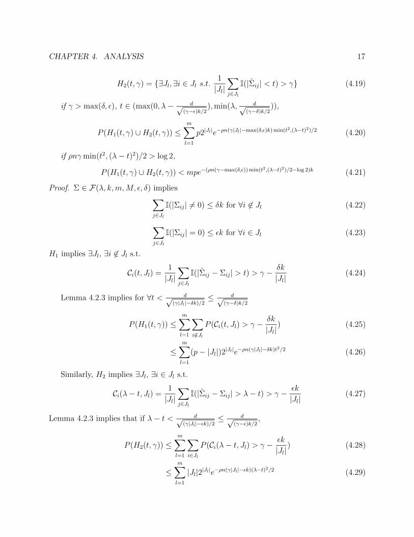
CHAPTER 4. ANALYSIS 17
H2(t, γ) = ∃Jl,∃i ∈ Jl s.t.1
|Jl|∑j∈Jl
I(|Σij| < t) > γ (4.19)
if γ > max(δ, ε), t ∈ (max(0, λ− d√(γ−ε)k/2
),min(λ, d√(γ−δ)k/2
)),
P (H1(t, γ) ∪H2(t, γ)) ≤m∑l=1
p2|Jl|e−ρn(γ|Jl|−max(δ,ε)k) min(t2,(λ−t)2)/2 (4.20)
if ρnγmin(t2, (λ− t)2)/2 > log 2,
P (H1(t, γ) ∪H2(t, γ)) < mpe−(ρn(γ−max(δ,ε)) min(t2,(λ−t)2)/2−log 2)k (4.21)
Proof. Σ ∈ F(λ, k,m,M, ε, δ) implies∑j∈Jl
I(|Σij| 6= 0) ≤ δk for ∀i 6∈ Jl (4.22)
∑j∈Jl
I(|Σij| = 0) ≤ εk for ∀i ∈ Jl (4.23)
H1 implies ∃Jl, ∃i 6∈ Jl s.t.
Ci(t, Jl) =1
|Jl|∑j∈Jl
I(|Σij − Σij| > t) > γ − δk
|Jl|(4.24)
Lemma 4.2.3 implies for ∀t < d√(γ|Jl|−δk)/2
≤ d√(γ−δ)k/2
P (H1(t, γ)) ≤m∑l=1
∑i/∈Jl
P (Ci(t, Jl) > γ − δk
|Jl|) (4.25)
≤m∑l=1
(p− |Jl|)2|Jl|e−ρn(γ|Jl|−δk)t2/2 (4.26)
Similarly, H2 implies ∃Jl, ∃i ∈ Jl s.t.
Ci(λ− t, Jl) =1
|Jl|∑j∈Jl
I(|Σij − Σij| > λ− t) > γ − εk
|Jl|(4.27)
Lemma 4.2.3 implies that if λ− t < d√(γ|Jl|−εk)/2
≤ d√(γ−ε)k/2
,
P (H2(t, γ)) ≤m∑l=1
∑i∈Jl
P (Ci(λ− t, Jl) > γ − εk
|Jl|) (4.28)
≤m∑l=1
|Jl|2|Jl|e−ρn(γ|Jl|−εk)(λ−t)2/2 (4.29)
CHAPTER 4. ANALYSIS 18
Combine the results, if γ > max(δ, ε) and t ∈ (max(0, λ− d√(γ−ε)k/2
),min(λ, d√(γ−δ)k/2
)),
P (H1(t, γ) ∪H2(t, γ)) ≤m∑l=1
p2|Jl|e−ρn(γ|Jl|−max(δ,ε)k) min(t2,(λ−t)2)/2 (4.30)
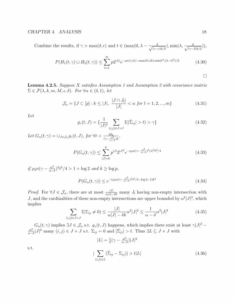
Lemma 4.2.5. Suppose X satisfies Assumption 1 and Assumption 2 with covariance matrixΣ ∈ F(λ, k,m,M, ε, δ). For ∀α ∈ (δ, 1), let
Jα = J ⊂ [p] : k ≤ |J |, |J ∩ Jl||J |
< α for l = 1, 2, ...,m (4.31)
Let
gγ(t, J) = 1
|J |2∑
(i,j)∈J×J
I(|Σij| > t) > γ (4.32)
Let Gα(t, γ) = ∪J∈Jαgγ(t, J), for ∀t < 2d2
(γ− α2
α−δ )k,
P (Gα(t, γ)) ≤p∑
|J |=k
p|J |2|J |2
e−ρ2n(γ− α2
α−δ )2|J |2t2/4 (4.33)
if ρ2n(γ − α2
α−δ )2t2/4 > 1 + log 2 and k ≥ log p,
P (Gα(t, γ)) ≤ e−(ρ2n(γ− α2
α−δ )2t2/4−log 2−1)k2 (4.34)
Proof. For ∀J ∈ Jα, there are at most |J |α|J |−δk many Jl having non-empty intersection with
J , and the cardinalities of these non-empty intersections are upper bounded by α2|J |2, whichimplies ∑
(i,j)∈J×J
I(Σij 6= 0) ≤ |J |α|J | − δk
α2|J |2 ≤ 1
α− δα2|J |2 (4.35)
Gα(t, γ) implies ∃J ∈ Jα s.t. gγ(t, J) happens, which implies there exist at least γ|J |2 −α2
α−δ |J |2 many (i, j) ∈ J × J s.t. Σij = 0 and |Σij| > t. Thus ∃L ⊆ J × J with
|L| = 12(γ − α2
α−δ )|J |2
s.t.|∑
(i,j)∈L
(Σij − Σij)| > t|L| (4.36)
CHAPTER 4. ANALYSIS 19
Apply Assumption 2 to v = ( 1√|J |
)Tj∈J , then for ∀t < d2|J ||L| = 2d2
(γ− α2
α−δ )|J |≤ 2d2
(γ− α2
α−δ )k,
P (gγ(t, J)) ≤(|J |2
|L|
)P (
1
|J ||∑
(i,j)∈L
(Σij − Σij)| >t|L||J |
) (4.37)
= 2|J |2
P (|vT (ΣL − ΣL)v| > t|L||J |
) (4.38)
≤ 2|J |2
e−ρ2n(t|L||J| )2 (4.39)
= 2|J |2
e−ρ2n(γ− α2
α−δ )2|J |2t2/4 (4.40)
By union bound
P (Gα(t, γ)) ≤∑J∈Jα
P (gγ(t, J)) (4.41)
≤p∑
|J |=k
(p
|J |
)2|J |
2
e−ρ2n(γ− α2
α−δ )2|J |2t2/4 (4.42)
≤p∑
|J |=k
p|J |2|J |2
e−ρ2n(γ− α2
α−δ )2|J |2t2/4 (4.43)
(4.44)
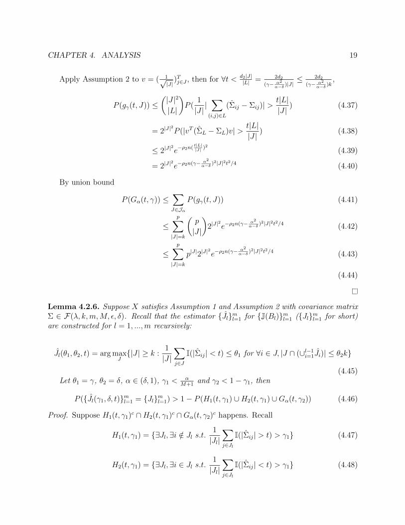
Lemma 4.2.6. Suppose X satisfies Assumption 1 and Assumption 2 with covariance matrixΣ ∈ F(λ, k,m,M, ε, δ). Recall that the estimator Jlml=1 for J(Bl)ml=1 (Jlml=1 for short)are constructed for l = 1, ...,m recursively:
Jl(θ1, θ2, t) = arg maxJ|J | ≥ k :
1
|J |∑j∈J
I(|Σij| < t) ≤ θ1 for ∀i ∈ J, |J ∩ (∪l−1i=1Ji)| ≤ θ2k
(4.45)Let θ1 = γ, θ2 = δ, α ∈ (δ, 1), γ1 <
αM+1
and γ2 < 1− γ1, then
P (Jl(γ1, δ, t)ml=1 = Jlml=1) > 1− P (H1(t, γ1) ∪H2(t, γ1) ∪Gα(t, γ2)) (4.46)
Proof. Suppose H1(t, γ1)c ∩H2(t, γ1)c ∩Gα(t, γ2)c happens. Recall
H1(t, γ1) = ∃Jl,∃i /∈ Jl s.t.1
|Jl|∑j∈Jl
I(|Σij| > t) > γ1 (4.47)
H2(t, γ1) = ∃Jl,∃i ∈ Jl s.t.1
|Jl|∑j∈Jl
I(|Σij| < t) > γ1 (4.48)

CHAPTER 4. ANALYSIS 20
Gα(t, γ2) = ∃J ∈ Jα s.t.1
|J |2∑i,j∈J
I(|Σij| > t) > γ2 (4.49)
θ1 = γ1, θ2 = δ andH2(t, γ1)c imply that for l = 1, 2, ...,m and for ∀i ∈ Jl, 1|Jl|∑
j∈Jl I(|Σij| <t) ≤ θ1, and |Jl ∩ (∪s 6=lJs)| ≤ θ2k. This implies that ∃Jlml=1 satisfying equation 4.45 s.t.
Jl ⊂ Jl for l = 1, 2, ...,m. Now it remains to show that Jlml=1 is indeed the unique solutionof 4.45:
Suppose ∃Jlml=1 satisfying 4.45 different from Jlml=1, then ∃J ∈ Jlml=1 s.t. J 6= Jl for∀l, thus one of following two cases must hold:
Case 1: ∃l s.t. |Jl ∩ J | ≥ α|J |, which contradicts H1(t, γ1)c if
α|J | − γ1|Jl| > θ1|J | (4.50)
Case 2: For ∀l, |Jl ∩ J | < α|J |, which contradicts Gα(t, γ2)c if
γ2|J |2 < (1− θ1)|J |2 (4.51)
If θ1 = γ, θ2 = δ, then conditions in Case 1 and Case 2 can be deduced to
γ1 <α
M + 1and γ2 < 1− γ1 (4.52)
Hence if condition 4.52 is satisfied, the event that ∃Jlml=1 different from Jlml=1 impliescontradiction, i.e. H1(t, γ1)c ∩H2(t, γ1)c ∩Gα(t, γ2)c implies that Jl(γ1, δ, t)ml=1 = Jlml=1 isthe unique solution of 4.45.
Lemma 4.2.7. (Amini and Wainwright (AW2009-1)) Consider the spike model Eβ definedin 2.11. If
n
k log(p− k)<
1 + β
β2(4.53)
Then the probability of error of any method is at least 12.
Proof. Refer to Amini and Wainwright (AW2009-1) Theorem 3.
Proof of Theorem 4.2.1:
Proof. Combine Lemma 4.2.4, Lemma 4.2.5, Lemma 4.2.6, if α ∈ (δ, 1), k ≥ log p, and

CHAPTER 4. ANALYSIS 21
γ1 <α
M + 1(4.54)
γ2 < 1− γ1 (4.55)
t ∈ (max(0, λ− d√(γ1 − ε)k/2
),min(λ,d√
(γ1 − δ)k/2)) (4.56)
t <2d2
(γ2 − α2
α−δ )k(4.57)
2 + log 2 < ρn(γ1 −max(δ, ε)) min(t2, (λ− t)2)/2 (4.58)
1 + log 2 < ρ2n(γ2 −α2
α− δ)2t2/4 (4.59)
then
P (Jl(γ1, δ, t)ml=1 6= Jlml=1) ≤ P (H1(t, γ1) ∪H2(t, γ1)) + P (Gα(t, γ2)) (4.60)
≤ mpe−[ρn(γ1−max(δ,ε)) min(t2,(λ−t)2)/2−log 2]k (4.61)
+ e−[ρ2n(γ2− α2
α−δ )2t2/4−log 2−1]k2 (4.62)
≤ e−[ρn(γ1−max(δ,ε)) min(t2,(λ−t)2)/2−log 2−2]k (4.63)
+ e−[ρ2n(γ2− α2
α−δ )2t2/4−log 2−1]k2 (4.64)
If t = λ2
= C2√n, and n
k2> C0 uniformly for all (n, k), then condition 4.57 is asymptotically
stronger than 4.56, i.e. 4.57 implies 4.56 for (n, k) big enough. Now conditions 4.54 – 4.59can be simplified as
1 > γ1 + γ2 (4.65)
α
M + 1> γ1 > max(ε, δ) +
8(2 + log 2)
ρC2(4.66)
α2
α− δ+
4d2
√n
Ck> γ2 >
α2
α− δ+
4√
1 + log 2
C√ρ2
(4.67)
Hence ∃γ1, γ2 satisfying 4.65 – 4.67 if ∃α ∈ (δ, 1) s.t.
1 > max(ε, δ) +8(2 + log 2)
ρC2+
4√
1 + log 2
C√ρ2
+α2
α− δ= A+
α2
α− δ(4.68)
α > (M + 1)(max(ε, δ) +8(2 + log 2)
ρC2) = B (4.69)
4d2
√n
Ck>
4√
1 + log 2
C√ρ2
(4.70)

CHAPTER 4. ANALYSIS 22
Note that M ≥ 1 and B ≥ 2δ. Since ddα
( α2
α−δ ) = (α−2δ)α(α−δ)2 > 0 for ∀α > 2δ, hence if
A+ B2
B−δ < 1, then ∃α ∈ (δ, 1) satisfying 4.68 and 4.69.
Thus if uniformly for all (k, n, p), k ≥ log p, λ = C√n, nk2> C0, and if
1 > A+B2
B − δ= max(ε, δ) +
8(2 + log 2)
ρC2+
4√
1 + log 2
C√ρ2
(4.71)
+(M + 1)2(max(ε, δ) + 8(2+log 2)
ρC2 )2
(M + 1)(max(ε, δ) + 8(2+log 2)ρC2 )− δ
(4.72)
d22n
k2>
1 + log 2
ρ2
(4.73)
then ∃γ1, γ2, α s.t. as (k, n, p)→∞,
P (Jl(γ1, δ,λ
2)ml=1 = Jlml=1)→ 1 (4.74)
This completes the proof of Upper Bound in Theorem 4.2.1.Note that Eβ with Γp−k = Ip−k×p−k is a subset of F(λ, k,m,M, ε, δ) with λ = β
k,m =
1,M = 1, ε = 0, δ = 0. Hence Lemma 4.2.7 with λ = βk
implies the Lower Bound in Theorem4.2.1.
Lemma 4.2.7 also suggests that nk log p
> 1+kλk2λ2
must hold in order to get perfect support
recovery. If 1+kλk2λ2
converges, one of following three cases must hold:
• 1+kλk2λ2→∞:
This implies kλ→ 0. Thus nk log p
> 1+kλk2λ2
if and only if λ2 = C2
n> log p
kn. Jl(γ1, δ,
λ2)ml=1
is rate optimal if k = O(log p) and nk2→∞.
• 1+kλk2λ2→ O(1):
This implies kλ→ O(1). It is rate optimal if k = O(log p) and n = O(k2).
• 1+kλk2λ2→ 0:
This implies kλ→∞, contradicting nk2> 1+log 2
ρ2d22. Hence no optimal rate is achieved.
4.3 Minimax Optimal Covariance Estimation
Theorem 4.2.1 shows that the support recovery estimator Jl(γ1, δ,λ2)ml=1 is rate optimal for
the specified range of parameters. After the block structure is recovered, we can estimate Σwith Σ∗ induced by Jlml=1 = Jl(γ1, δ,
λ2)ml=1:
Σ∗ij = ΣijI((i, j) ∈ ∪ml=1Jl × Jl) (4.75)

CHAPTER 4. ANALYSIS 23
Next theorem shows Σ∗ is minimax optimal in spectral norm for class F(λ, k,m,M, ε, δ) withparameters in the specified range.
Theorem 4.3.1. Suppose i.i.d mean 0 p-variate sub-Gaussian X1, ..., Xn satisfy Assumption1 and Assumption 2, with covariance matrix Σ ∈ F(λ, k,m,M, ε, δ).
If k = O(log p), λ = C√n, nk2> 1+log 2
ρ2d22, and
max(ε, δ) +8(2 + log 2)
ρC2+
4√
1 + log 2
C√ρ2
+(M + 1)2(max(ε, δ) + 8(2+log 2)
ρC2 )2
(M + 1)(max(ε, δ) + 8(2+log 2)ρC2 )− δ
< 1 (4.76)
Then
infΣ
supΣ∈F(λ,k,m,M,ε,δ)
E‖ Σ− Σ‖2 k
n(4.77)
Proof. The proof of Theorem 4.3.1 consists of two parts: Lemma 4.3.3 shows the upperbound, and Lemma 4.3.5 shows the lower bound.
Following are lemmas relevant to the proof of Theorem 4.3.1.
Lemma 4.3.2. (T. Cai et al (CZZ2010-1)) For any k dimensional sub-Gaussian r.v. withcovariance matrix Σk with largest eigenvalue upper bounded uniformly for all k, ∃ρ3 s.t. for∀t < ρ3,
P (‖Σk − Σk‖ > t) < 5ke−ρ3nt2
(4.78)
Proof. Refer to T. Cai et al (CZZ2010-1) Lemma 3.
Lemma 4.3.3. Suppose all assumptions in Theorem 4.3.1 hold. Recall Σ∗ is induced byJlml=1:
Σ∗ij = ΣijI((i, j) ∈ ∪ml=1Jl × Jl) (4.79)
Then ∃C0, C1 > 0 s.t. if k > C0 log p, then
supΣ∈F(λ,k,m,M,ε,δ)
E[‖Σ∗ − Σ‖2] ≤ C1Mk
n(4.80)
Proof. Denote A = Jlml=1 = Jlml=1,
E[‖Σ∗ − Σ‖2] = E[‖Σ∗ − Σ‖2(IA + IAc)] (4.81)
Recall that by construction of the blocks, ∃ partition L1 t L2 = [m] s.t. Ji ∩ Jj = ∅ for∀(i, j) ∈ (L1 × L1) ∪ (L2 × L2), this implies
‖Σ∗ − Σ‖IA ≤ ‖∑l∈L1
ΣJl×Jl − ΣJl×Jl‖+ ‖∑l∈L2
ΣJl×Jl − ΣJl×Jl‖ (4.82)
≤ maxl∈L1
‖ΣJl×Jl − ΣJl×Jl‖+ maxl∈L2
‖ΣJl×Jl − ΣJl×Jl‖ (4.83)
≤ 2 maxl=1,...,m
‖ΣJl×Jl − ΣJl×Jl‖ (4.84)

CHAPTER 4. ANALYSIS 24
Denote N (m) = maxl=1,...,m ‖ΣJl×Jl − ΣJl×Jl‖. Let B = N (m) > t. Lemma 4.3.2 implies
P (B) = P ( maxl=1,...,m
‖ΣJl×Jl − ΣJl×Jl‖ > t) (4.85)
≤ m maxl=1,...,m
P (‖ΣJl×Jl − ΣJl×Jl‖ > t) (4.86)
< m5Mke−ρ3nt2
(4.87)
Let t = c1
√Mkn
withc212> log 5
ρ3, then ∃c2 > 0 s.t.
E[‖Σ∗ − Σ‖2IA] ≤ 4E[(N (m))2(IB + IBc)] (4.88)
≤ 4E[t2 + (N (m))2IB] (4.89)
≤ 4(t2 +√E[(N (m))4]P (B)) (4.90)
≤ 4(t2 + (Mk)2m5Mke−ρ3nt2/2) (4.91)
≤ c2Mk
n(4.92)
Recall that Theorem 4.2.1 implies if assumptions in Theorem 4.3.1 hold, then ∃c3 > 0 s.t.P (A) < e−c3k. Thus if C0 >
4c3
and k ≥ C0 log p,
E[‖Σ∗ − Σ‖2IAc ] ≤√E[‖Σ∗ − Σ‖4]P (Ac) (4.93)
≤ p4e−c3k (4.94)
≤ p−(C0c3−4) (4.95)
Combine the results, ∃C0, C1 s.t. if k > C0 log p, then
E[‖Σ∗ − Σ‖2] = E[‖Σ∗ − Σ‖2(IA + IAc)] (4.96)
≤ c2Mk
n+ p−(C0c3−4) (4.97)
≤ C1Mk
n(4.98)
Lemma 4.3.4. (Generalized Fano’s Lemma, B. Yu (Y1997-1)) Let Mr ⊂ P contains rprobability measures such that for all i 6= j with i, j ≤ r
d(θ(Pi), θ(Pj)) ≥ αr (4.99)
andD(Pi‖Pj) ≤ βr (4.100)

CHAPTER 4. ANALYSIS 25
where D(Pi‖Pj) denotes the Kullback-Leibler(K-L) divergence of Pj from Pi,
D(Pi‖Pj) =
∫ln(
dPidPj
)dPi (4.101)
Then
maxiEPi [d(θ, θ(Pi))] ≥
αr2
(1− βr + log 2
log r) (4.102)
Proof. Refer to Assouad, Fano, and Le Cam by Bin Yu (Y1997-1).
Lemma 4.3.5. If λ = C√n
with C <√
log p2k
, then
infΣ
supΣ∈F(λ,k,m,M,ε,δ)
E[‖Σ− Σ‖2] ≥ C2Mk
16n(4.103)
Proof. Let r =(pk
), denote the set of all subsets of 1, ..., p with k elements by
S = Li ⊂ 1, ..., p : |Li| = k for i = 1, ..., r (4.104)
Denote Bi ∈ Rp×p a block matrix with block index Li,
(Bi)jl = I(j, l ∈ Li, j 6= l) (4.105)
and Di ∈ Rp×p a diagonal block matrix,
(Di)jl = I(j, l ∈ Li, j = l) (4.106)
Consider Pi the join distribution of n i.i.d. p−dimensional Gaussian with covariance matrixIp×p + λBi
Mr = Pi : Σ(Pi) = Ip×p + λBi for i = 1, ..., r (4.107)
Denote Σi = Σ(Pi), consider d = ‖.‖ the operator norm, then for ∀i 6= j
d(Σi,Σj) = ‖Σi − Σj‖ ≥ λ√k − 1 (4.108)
We have αr = λ√k − 1.
Now we derive an upper bound for the KL divergence
D(Pj‖Pi) =n
2[tr(ΣjΣ
−1i )− log det(ΣjΣ
−1i )− p] (4.109)
Note det(Σi) = det(Σj) since Σi is just a reordering of Σj. Thus log det(ΣjΣ−1i ) = 0. Also
note Σ−1i = Ip×p − yBi + (x− 1)Di with
x =1 + λ(k − 2)
1 + λ(k − 2)− λ2(k − 1)(4.110)

CHAPTER 4. ANALYSIS 26
y =λ
1 + λ(k − 2)− λ2(k − 1)(4.111)
Now suppose |Bi ∩Bj| = s, we have
tr(ΣjΣ−1i ) = x(k − s) + (x− λy(s− 1))s+ k − s+ p− (2k − s) (4.112)
= p− k + xk − λys(s− 1) (4.113)
≤ p+ k(x− 1) (4.114)
Hence
D(Pj‖Pi) ≤n
2k(x− 1) (4.115)
=nλ2k(k − 1)
2(1 + λ(k − 2)− λ2(k − 1))(4.116)
= βr (4.117)
By the generalized Fano’s Lemma
maxiEPi [d(θ, θ(Pi))] ≥
αr2
(1− βr + log 2
log r) (4.118)
=λ√k − 1
2(1−
nλ2k(k−1)2(1+λ(k−2)−λ2(k−1))
+ log 2
log(pk
) ) (4.119)
≥ λ√k
2(1− c′ nλ2k2
(1 + λk − λ2k)k log p) (4.120)
Note 11+λk−λ2k < 1. λ = C√
nimplies
nλ2k
(1 + λk − λ2k) log p≤ C2k
log p(4.121)
E[‖.‖2] ≥ E[‖.‖]2 and the block size is upper bounded by Mk implies that if C <√
log p2k
,
then
infΣ
supΣ∈F(λ,k,m,M,ε,δ)
E[‖Σ− Σ‖2] ≥ (λ√Mk
4)2 ≥ C2Mk
16n(4.122)
4.4 Algorithm Correctness and Computational
Complexity
The last theorem of this chapter analyzes success probability and computational complexityof algorithm FBAll().

CHAPTER 4. ANALYSIS 27
Theorem 4.4.1. Suppose X satisfies Assumption 1 and Assumption 2, with covariancematrix Σ ∈ F(λ, k,m,M, ε, δ). If λ = C√
n, k ≥ log p, n
k2> 4
ρ2d22, and if
M <1− 3 max(ε, δ)
2 max(ε, δ)(4.123)
C > max(8
√ρ2((1−δ
2)2 − ε
2), 4(M + 1)
√log 2
(1− δ)ρ) (4.124)
then there exists γ1, γ2, η s.t. FBAll(A, k, s = ηk − 1, θb = 1 − ε − γ2, θr = 1 − γ1, t) withinput matrix A = (I(|Σij| > λ
2))1≤i,j≤p has output Jlm
′
l=1 satisfying
P (Jlm′
l=1 6= Jlml=1) ≤ mpe−[ρn(γ1η−max(δ,ε))λ2/8−log 2(η+M)]k (4.125)
+ p2e−[(ρ2nγ22λ2/16−log 2)k−2 log p]k (4.126)
→ 0 (4.127)
Furthermore, for probability at least
1− 2
p− 1→ 1 (4.128)
the worst case computational complexity of the algorithm FBAll() is
O(2s(s log p)s/2kps+2e−(ρC2/8−log 2)s(s+1)/4)
with s = ηk − 1.
Remark: In general η is a constant, and s = ηk = O(log p). This makes the algorithmrunning in exponential time asymptotically. However the constant C has to be large enoughto make the problem statistically identifiable, and that makes the algorithm very efficient inpractice for a reasonably large range of p. For p equal to several thousands, s is usually 0 or1. For the case s = 0, the computation complexity is essentially O(p2k). We will illustratethis point in simulation experiments in next chapter.
Lemma 4.4.2. Suppose X satisfies Assumption 1 with covariance matrix Σ,
Σ ∈ F(λ, k,m,M, ε, δ)
For t ∈ (0, λ), let
H1(t, γ, η) = ∃Jl,∃i /∈ Jl,∃J ⊂ Jl s.t. |J | ≥ ηk,1
|J |∑j∈J
I(|Σij| > t) > γ (4.129)
H2(t, γ, η) = ∃Jl,∃i ∈ Jl,∃J ⊂ Jl s.t. |J | ≥ ηk,1
|J |∑j∈J
I(|Σij| < t) > γ (4.130)

CHAPTER 4. ANALYSIS 28
if γη > max(δ, ε), t ∈ (max(0, λ− d√(γη−ε)k/2
),min(λ, d√(γη−δ)k/2
)),
P (H1(t, γ, η) ∪H2(t, γ, η)) ≤m∑l=1
p2|Jl|maxJ⊂Jl
2|J |e−ρn(γ|J |−max(δ,ε)k) min(t2,(λ−t)2)/2 (4.131)
and if ηη+M
ρnγmin(t2, (λ− t)2)/2 > log 2,
P (H1(t, γ, η) ∪H2(t, γ, η)) < mpe−[ρn(γη−max(δ,ε)) min(t2,(λ−t)2)/2−log 2(η+M)]k (4.132)
Proof. Similar to the proof of Lemma 4.2.4, for ∀t < d√(γ|J |−δk)/2
≤ d√(γη−δ)k/2
P (H1(t, γ, η)) ≤m∑l=1
∑i/∈Jl
∑J⊂Jl
P (Ci(t, J) > γ − δk
|J |) (4.133)
≤m∑l=1
(p− |Jl|)2|Jl|maxJ⊂Jl
2|J |e−ρn(γ|J |−δk)t2/2 (4.134)
and if λ− t < d√(γ|J |−εk)/2
≤ d√(γη−ε)k/2
,
P (H2(t, γ, η)) ≤m∑l=1
∑i∈Jl
∑J⊂Jl
P (Ci(λ− t, J) > γ − εk
|J |) (4.135)
≤m∑l=1
|Jl|2|Jl|maxJ⊂Jl
2|J |e−ρn(γ|J |−εk)(λ−t)2/2 (4.136)
Thus if γη > max(δ, ε), t ∈ (max(0, λ− d√(γη−ε)k/2
),min(λ, d√(γη−δ)k/2
)),
P (H1(t, γ, η) ∪H2(t, γ, η)) ≤m∑l=1
p2|Jl|maxJ⊂Jl
2|J |e−ρn(γ|J |−max(δ,ε)k) min(t2,(λ−t)2)/2 (4.137)
if ρnγmin(t2, (λ− t)2)/2 > log 2η+Mη
,
P (H1(t, γ, η) ∪H2(t, γ, η)) < mpe−[ρn(γη−max(δ,ε)) min(t2,(λ−t)2)/2−log 2(η+M)]k (4.138)
Lemma 4.4.3. Suppose X satisfies Assumption 1 and Assumption 2 with covariance matrixΣ ∈ F(λ, k,m,M, ε, δ). Let
G(t, γ, s, w) = ∃J, L s.t. |J | ≥ s, |L| ≥ w,1
|J ||L|∑
j∈J,l∈L
I(|Σjl − Σjl| > t) > γ (4.139)
if (ρ2nγ2t2/4− log 2) min(s, w) > 2 log p, for ∀t < 2d2
γ√|J ||L|
,
P (G(t, γ, s, w)) ≤ p2e−[(ρ2nγ2t2/4−log 2) min(s,w)−2 log p] max(s,w) (4.140)

CHAPTER 4. ANALYSIS 29
Proof. Similar to the proof of Lemma 4.2.5, if
(ρ2nγ2t2/4− log 2) min(s, w) > 2 log p
for ∀t < 2d2
γ√|J ||L|
,
P (G(t, γ, s, w)) ≤p∑|J |=s
p∑|L|=w
(p
|J |
)(p
|L|
)P (
1√|J ||L|
∑j∈J,l∈L
I(|Σjl − Σjl| > t) > γ√|J ||L|)
(4.141)
≤p∑|J |=s
p∑|L|=w
p|J |+|L|2|J ||L|e−ρ2n|J ||L|γ2t2/4 (4.142)
≤ p2e−[(ρ2nγ2t2/4−log 2) min(s,w)−2 log p] max(s,w) (4.143)
Lemma 4.4.4. Define: A zero-mean random variable Y is sub-exponential if ∃d > 0 s.t.
E[etY ] ≤ ∞ for ∀|t| ≤ d (4.144)
Claim: Y is sub-exponential if and only if ∃ρ′, d′ s.t. E[exp(tY )] ≤ exp( t2ρ′
2) for ∀|t| < d′.
Proof. For t close to 0,
E[etY ] = 1 +t2E[Y 2]
2+ o(t2) (4.145)
et2ρ′2 = 1 +
t2ρ′
2+ o(t2) (4.146)
Hence if ρ′ > E[Y 2], then ∃d′ s.t. E[exp(tY )] ≤ exp( t2ρ′
2) for ∀|t| < d′.
Lemma 4.4.5. Suppose X satisfies Assumption 1 and Assumption 2. Let
D(t, J, L) =1
|J |∑j∈J
∏i∈L
I(|Σij − Σij| > t) (4.147)
Then ∃d3 > 0 s.t. for ∀|t′| < d3,
P (|D(t, J, L)− E[D(t, J, L)]| > t′) < 2e−t′22e(ρnt
2/2−log 2)|L|(4.148)
Furthermore, let
G(t′, t, s) = ∃L s.t. |L| = s, |D(t, [p], L)− E[D(t, [p], L)]| > t′ (4.149)
then
P (G(t′, t, s)) < 2pse−t′22e(ρnt
2/2−log 2)s
(4.150)

CHAPTER 4. ANALYSIS 30
Proof. For ∀t <√
2d√|L|
, Assumption 1 implies
E[D(t, J, L)] ≤ maxj∈J
E[∏i∈L
I(|Σij − Σij| > t)] (4.151)
= maxj∈J
P (∑i∈L
|Σij − Σij| > |L|t) (4.152)
< e−(ρnt2/2−log 2)|L| (4.153)
Similarly
E[D(t, J, L)2] < maxj1,j2∈J
E[∏i∈L
I(|Σij1 − Σij1| > t)∏i∈L
I(|Σij2 − Σij2 | > t)] (4.154)
= maxj∈J
P (∑i∈L
|Σij − Σij| > |L|t) (4.155)
< e−(ρnt2/2−log 2)|L| (4.156)
Let Y = D(t, J, L)− E[D(t, J, L)]. Generalization of Holder’s inequality implies
E[exp(τY )] = E[exp(τD(t, J, L)− τE[D(t, J, L)])] (4.157)
= exp(−τE[D(t, J, L)])E[exp(τD(t, J, L))] (4.158)
≤ E[∏j=J
exp(τ
|J |∏i∈L
I(|Σij − Σij| > t))] (4.159)
≤∏j∈J
E[exp(τ∏i∈L
I(|Σij − Σij| > t))]1|J| (4.160)
≤ maxj∈J
eτP (∑i∈L
|Σij − Σij| > |L|t) + 1 (4.161)
<∞ (4.162)
Hence Y is sub-exponential and E[Y 2] < E[D(t, J, L)2] < e−(ρnt2/2−log 2)|L|, Lemma 4.4.4implies that ∃d3 > 0 s.t. for ∀|t′| < d3,
P (|D(t, J, L)− E[D(t, J, L)]| > t′) = P (|Y | > t′) < 2e−t′22e(ρnt
2/2−log 2)|L|(4.163)
Union bound implies the upper bound of P (G(t′, t, s)).
Proof of Theorem 4.4.1:
Proof. Suppose H1(λ2, γ1, η)c∩H2(λ
2, γ1, η)c∩G(λ
2, γ2, k, k)c happens with γ1, γ2 to be chosen
later. Recall the input matrix A = (I(|Σij| > λ2))1≤i,j≤p. Denote Jlm
′
l=1 the output of

CHAPTER 4. ANALYSIS 31
algorithm FBAll(A, k, s, θb, θr, t). Each Jl is an output of FBRec(A,L, ∅, k, s, θb, θr, t) withL = [p] initially. By construction of the algorithm, Jl satisfies
|Jl| ≥ k (4.164)
1
|Jl|
∑j∈Jl
Aij ≥ θr for ∀i ∈ Jl (4.165)
1
|Jl|2∑i,j∈Jl
Aij ≥ θb (4.166)
Similar to the proof of Lemma 4.2.6, if following holds:
1− δ2−Mγ1 ≥ (1− θr) (4.167)
2(1− δ
2)2 − γ2 ≥ 1− θb (4.168)
1− γ1 ≥ θr (4.169)
max(1− γ1, 1− ε− γ2) ≥ θb (4.170)
then H1(λ2, γ1, η)c ∩ H2(λ
2, γ1, η)c ∩ G(λ
2, γ2, k, k)c implies that there exists some l′ s.t. Jl ⊂
Jl′ = J(Bl′). Thus if
θr = 1− γ1 (4.171)
θb = max(1− γ1, 1− ε− γ2) (4.172)
γ1 ≤1− δ
2(M + 1)(4.173)
γ2 ≤ max((1− δ
2)2 − ε
2, 2(
1− δ2
)2 − γ1) (4.174)
then FBRec() does not recover any wrong block and always recovers correct sub-blocks. Itremains to show that it indeed finds all the blocks with full size.
Calling FBAll(A, k, s, θb, θr, t) would eventually call FB(A, J, k, t) with |J | = s + 1.Suppose J ⊂ Jl = J(Bl) for some l, and J ∩ ∪i 6=lJi = ∅, which at some step always happensif s < (1− δ)k − 1 and since FBAll() exhaustively search over all J satisfying
Aij 6= 0 for ∀i 6= j ∈ J (4.175)
If s+ 1 ≥ ηk, then H1(λ2, γ1, η)c ∩H2(λ
2, γ1, η)c implies that∑
j∈J
I(|Σij| >λ
2) > (1− γ1)|J | for ∀i ∈ J (4.176)
∑j∈J
I(|Σij| >λ
2) < γ1|J | for ∀i 6∈ J (4.177)

CHAPTER 4. ANALYSIS 32
If γ1 <12, then the output J0 of FB(A, J, k, t) satisfies |J0| = k and J0 ⊂ Jl. By the same
reasoning, FBS(A, J0, θb, θr, t) recovers the full size of Jl with θr, θb defined in 4.171 and4.172. This shows the correctness of the algorithm if event H1(λ
2, γ1, η)c ∩ H2(λ
2, γ1, η)c ∩
G(λ2, γ2, k, k)c happens.
To bound the error probability of FBAll(), Lemma 4.4.2 and Lemma 4.4.3 implies thatif
γ1η > max(δ, ε) (4.178)
λ
2∈ (max(0, λ− d√
(γ1η − ε)k/2),min(λ,
d√(γ1η − δ)k/2
)) (4.179)
log 2 <η
η +Mρnγ1λ
2/8 (4.180)
log p
k< ρ2nγ
22λ
2/32− log 2/2 (4.181)
λ
2<
2d2
γ2k(4.182)
then
P (H1(λ
2, γ1, η) ∪H2(
λ
2, γ1, η) ∪G(
λ
2, γ2, k, k)) ≤ mpe−[ρn(γ1η−max(δ,ε))λ2/8−log 2(η+M)]k
(4.183)
+ p2e−[(ρ2nγ22λ2/16−log 2)k−2 log p]k (4.184)
→ 0 (4.185)
Combining 4.171 – 4.174 and 4.178 – 4.182, and λ = C√n, k ≥ log p, we have
θr = 1− γ1 (4.186)
θb = max(1− γ1, 1− ε− γ2) (4.187)
max(max(ε, δ)
η,8 log 2(η +M)
ρC2η) < γ1 ≤
1− δ2(M + 1)
(4.188)
8√ρ2C
< γ2 ≤ min(4d2
√n
Ck, (
1− δ2
)2 − ε
2) (4.189)
where 4.188 and 4.189 are equivalent to
η >2(M + 1) max(ε, δ)
1− δ(4.190)
η >M(M + 1)16 log 2
ρC2(1− δ)− (M + 1)16 log 2(4.191)
√n
k>
2
d2√ρ2
(4.192)
C >8
√ρ2((1−δ
2)2 − ε
2)
(4.193)

CHAPTER 4. ANALYSIS 33
Thus if λ = C√n, k ≥ log p, n
k2> 4
ρ2d22, and if
M <1− 3 max(ε, δ)
2 max(ε, δ)(4.194)
C > max(8
√ρ2((1−δ
2)2 − ε
2), 4(M + 1)
√log 2
(1− δ)ρ) (4.195)
then there exists γ1, γ2, η s.t. FBAll(A, k, s = ηk−1, θb = 1− ε−γ2, θr = 1−γ1, t) perfectlyrecovers Jlml=1 with probability going to 1.
Next we calculate the computation complexity of FBRec(). Suppose ∩si=1G(t′i,λ2, i)c
happens with t′i satisfying
t′i = 2√i log pe−(ρnλ2/8−log 2)i/2 (4.196)
= 2√i log p∆i (4.197)
where ∆ = e−(ρnλ2/8−log 2)/2. Recall that FBAll() searches over all J ∈ J (s+ 1) defined as
J (s+ 1) = J : |J | = s+ 1, Aij 6= 0 for ∀i 6= j ∈ J (4.198)
For each J , FB() takes O(pk). Hence FBAll() takes O(|J (s+ 1)|pk) with
|J (s+ 1)| = ps∏i=1
(pt′i) (4.199)
≤ 2s(s log p)s/2ps+1∆s(s+1)/2 (4.200)
Hence the overall worst case computational complexity for FBAll() is
O(2s(s log p)s/2kps+2∆s(s+1)/2)
For the case s = 0, the dominant term is O(kp2). Furthermore, this is true with probabilityat least
P (∩si=1G(t′i,λ
2, i)c) ≥ 1− 2
s∑i=1
pie−t′2i2e(ρnt
2/2−log 2)i
(4.201)
≥ 1− 2s∑i=1
p−i (4.202)
≥ 1− 2
p− 1→ 1 (4.203)
CHAPTER 5. EXPERIMENT 34
Chapter 5
Experiment
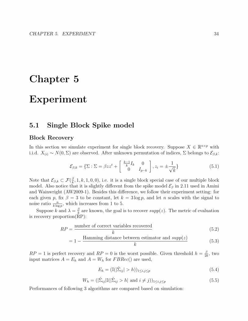
5.1 Single Block Spike model
Block Recovery
In this section we simulate experiment for single block recovery. Suppose X ∈ Rn×p withi.i.d. X(i) ∼ N(0,Σ) are observed. After unknown permutation of indices, Σ belongs to Eβ,k:
Eβ,k = Σ : Σ = βzzt +
[k−1kIk 0
0 Ip−k
], zi = ± 1√
k (5.1)
Note that Eβ,k ⊂ F(βk, 1, k, 1, 0, 0), i.e. it is a single block special case of our multiple block
model. Also notice that it is slightly different from the spike model Eβ in 2.11 used in Aminiand Wainwright (AW2009-1). Besides this difference, we follow their experiment setting: foreach given p, fix β = 3 to be constant, let k = 3 log p, and let n scales with the signal tonoise ratio n
k log p, which increases from 1 to 5.
Suppose k and λ = βk
are known, the goal is to recover supp(z). The metric of evaluationis recovery proportion(RP):
RP =number of correct variables recovered
k(5.2)
= 1− Hamming distance between estimator and supp(z)
k(5.3)
RP = 1 is perfect recovery and RP = 0 is the worst possible. Given threshold h = β2k
, twoinput matrices A = Eh and A = Wh for FBRec() are used,
Eh = (I(|Σij| > h))1≤i,j≤p (5.4)
Wh = (|Σij|I(|Σij > h| and i 6= j))1≤i,j≤p (5.5)
Performances of following 3 algorithms are compared based on simulation:

CHAPTER 5. EXPERIMENT 35
Figure 5.1: DSPCA: 20 iterations average RP with input matrix Σ
• DSPCA: Use Σ as input matrix. Take eigen-decomposition of the output matrix ofDSPCA, pick top k largest entries in absolute value of the eigenvector correspondingto the largest eigenvalue.
• FBRec(0): s = 0. Use A = Eh or Wh as input matrix. Let L = [p], J = ∅, k is given,θr, θb as chosen in Theorem 4.4.1, t = 10.
• FBRec(1): s = 1. Use A = Eh or Wh as input matrix. Let L = [p], J = ∅, k is given,θr, θb as chosen in Theorem 4.4.1, t = 10.
Note that FBRec(0) with s = 0 is similar to TPower by X.T. Yuan and T. Zhang (YZ2011-1).For dimension p = 500, 1000, 1500, 2000, average RP over 20 iterations are reported in Fig-ure 5.1, Figure 5.2, Figure 5.3. As shown by the result, input Wh indeed is better thaninput Eh for both FBRec(0) and FBRec(1), while FBRec(0) is more sensitive to dimensionincrement. The average running time for various algorithm is reported in Table 5.1. As therunning time for DSPCA does not depend on the signal to noise ratio(SNR) n
k log p, for each
dimension p the average running time over all SNR is reported. Notice that the runningtime for both FBRec(0) and FBRec(1) heavily depends on SNR, i.e. for fixed dimension p,FBRec() runs faster for larger SNR.
Covariance Estimation
As in previous section, suppose the same data X is observed with known k and β. Nextgoal is covariance estimation in spectral norm. Denote Σ as the generic estimator, the

CHAPTER 5. EXPERIMENT 36
Figure 5.2: FBRec(0): 20 iterations average RP with s = 0, input matrix Wh and Eh
Figure 5.3: FBRec(1): 20 iterations average RP with s = 1, input matrix Wh and Eh

CHAPTER 5. EXPERIMENT 37
p nk log p
DSPCA FBRec(0) FBRec(1)
500 1 16.6 0.0217 0.0805500 2 16.6 0.0055 0.0112500 3 16.6 0.0037 0.0045500 4 16.6 0.0022 0.0023500 5 16.6 0.0020 0.00201000 1 106.9 0.3048 0.61231000 2 106.9 0.0328 0.05581000 3 106.9 0.0153 0.01871000 4 106.9 0.0079 0.00801000 5 106.9 0.0059 0.00581500 1 331.1 1.2577 1.79021500 2 331.1 0.1038 0.13651500 3 331.1 0.0364 0.03831500 4 331.1 0.0167 0.01761500 5 331.1 0.0122 0.01222000 1 899.2 3.9335 4.44272000 2 899.2 0.2647 0.43752000 3 899.2 0.0788 0.08752000 4 899.2 0.0354 0.04652000 5 899.2 0.0199 0.0191
Table 5.1: Average run time in seconds over 20 iterations
performances is evaluated based on the spectral norm of the difference between the truth Σand the estimator Σ:
‖∆‖ = ‖Σ− Σ‖
Following 3 estimators are compared:
• Oracle: As if the permutation is known, keep entries of Σ within the block and on thediagonal, and make all the other entries 0.
• Block estimate: Use FBRec() to recover the block, keep entries of Σ within the esti-mated block and on the diagonal, make every other entries 0.
• Threshold: Pick threshold h that minimizes ‖∆‖, then estimate Σ by Th(Σ).
For dimension p = 500, 1000, 1500, 2000, average ‖∆‖ over 20 iterations for above estimatorsare reported in Figure 5.4.

CHAPTER 5. EXPERIMENT 38
Figure 5.4: 20 iteration average ‖∆‖: spectral norm of difference between the populationand the estimator

CHAPTER 5. EXPERIMENT 39
p nk log p
2 3 4 5
500 9.71 4.92 5.19 5.241000 41.69 27.89 29.41 30.441500 147.21 112.25 75.02 78.402000 248.43 156.84 158.38 165.79
Table 5.2: FBAll(): 30 iteration average run time in seconds. SNR scale nk log p
.
5.2 Multiple Block Model
In this section we simulate experiments for multiple blocks recovery and covariance estima-tion. Suppose X ∈ Rn×p with i.i.d. X(i) ∼ N(0,Σ) are observed. Σ ∈ F(λ, k,m,M, ε, δ).Same as previously, consider p = 500, 1000, 1500, 2000. For each given p, let k = 3 log p, λ =3k,M = 2,m = p/(Mk), ε = δ = 0.1, and n scales with n
k log pwhich increases from 2 to 5. The
size of each block is uniformly random from [k,Mk] = [k, 2k]. Given estimator Jlm′
l=1 of thetrue blocks Jlml=1, the performance of support recovery is evaluated by multiple recoveryproportion(MRP):
MRP =1
m+m′(m∑l=1
m′
maxi=1
|Jl ∩ Ji||Jl|
+m′∑i=1
mmaxl=1
|Jl ∩ Ji||Ji|
) (5.6)
MRP can be considered as average RP over all Jlml=1 and Jlm′
l=1. MRP = 1 if andonly if perfect recovery Jlml=1 = Jlm
′
l=1 with m = m′. MRP = 0 is the worst possible.FBAll(A, k, s, θb, θr, t) is used for support recovery, where A = Wh with h = λ
2= 3
2k, k
is given, s = 1, θb, θr as in Theorem 4.4.1, t = 10. 30 iteration average MRP is reportedin Figure 5.5. The average running time for FBAll() is reported in Table 5.2. Same asprevious section, the three estimators: oracle, block estimate and threshold are compared interms of spectral norm of the difference to the truth. 30 iteration average ‖∆‖ for the threeestimators are reported in Figure 5.7.
Next we use different SNR scale, i.e. for each given p, let n = 3k log p = 9(log p)2, λ = C√n
with C increasing from 2 to 5, and keep everything else unchange. Again use FBAll() forsupport recovery, with Wh and h = λ
2= C
2√n, and keep all other setting the same. Use
the same three estimators to estimate Σ. 30 iteration average MRP for support recovery isreported in Figure 5.6. Average running time for FBAll() is reported in Table 5.3. And30 iteration average ‖∆‖ is reported in Figure 5.8. As shown by both experiments, perfectblock recovery implies that the block estimate agrees with the oracle for large enough signalstrength.

CHAPTER 5. EXPERIMENT 40
p C 2 3 4 5
500 12.53 5.31 5.41 6.371000 73.83 27.81 29.85 34.781500 182.81 74.65 77.66 81.142000 284.54 153.46 156.37 160.53
Table 5.3: FBAll(): 30 iteration average run time in seconds. SNR scale C = λ√n.
Figure 5.5: 30 iteration average MRP for FBAll with input matrix Wh. SNR scale nk log p
.
Figure 5.6: 30 iteration average MRP for FBAll with input matrix Wh. SNR scale C = λ√n.

CHAPTER 5. EXPERIMENT 41
Figure 5.7: 30 iteration average ‖∆‖: spectral norm of difference between the populationand the estimator. SNR scale n
k log p.

CHAPTER 5. EXPERIMENT 42
Figure 5.8: 30 iteration average ‖∆‖: spectral norm of difference between the populationand the estimator. SNR scale C = λ
√n.

CHAPTER 5. EXPERIMENT 43
5.3 Application
In this section we apply the block recovery algorithm to the so called entity resolutionproblem to identify whether data objects from different sources represent the same entity.This problem is also known as record matching (P2002-1) (F2009-1), record linkage (N1959-1)(F1969-1) (B2004-1), or deduplication (B2003-1) (BG2004-1). Given data B ∈ Rn×p, eachobject is represented by a sparse n vector and there are p objects. Bij ≥ 0 for all i, j. Thecosine similarity A ∈ Rp×p is defined as
Aij =BtiBj√
‖Bi‖2‖Bj‖2
(5.7)
This is following the setup in L.C. Shu et al (S2011-1).The goal is to partition indices of Ainto blocks such that similarity Aij is large for i, j within the same block, and Aij is smallfor i, j from different blocks. This type of data is not what we have studied up to now, butour algorithm is directly applicable. We compare following two algorithms:
• SPAN proposed by L.C. Shu et al (S2011-1): The idea is to use spectral clusteringto recursively bi-partition the indices and stop while Newman-Girvan modularity isnegative.
• FB: Run FBAll(A, k, s, θb, θr, t) with parameters k = 10, s = 0, θb = 0.5, θr = 0.4.
We apply these two algorithms to a data set from Alcatel Lucent with A ∈ Rp×p for p = 3000.This is a randomly picked subset of the data used in L.C. Shu et al (S2011-1). The originalsimilarity matrix is plotted in Figure 5.9. The similarity matrix permuted by SPAN is plottedin Figure 5.10. The similarity matrix permuted by FB is plotted in Figure 5.11. Figure 5.12,Figure 5.13 and Figure 5.14 are a closer look to sub-matrices of similarity matrix permutedby FB.

CHAPTER 5. EXPERIMENT 44
Figure 5.9: Original similarity matrix, each entry multiplied by 60
Figure 5.10: Similarity matrix permuted by SPAN, each entry multiplied by 60

CHAPTER 5. EXPERIMENT 45
Figure 5.11: Similarity matrix permuted by FB, each entry multiplied by 60
Figure 5.12: Sub-matrix of similarity matrix permuted by FB, each entry multiplied by 60

CHAPTER 5. EXPERIMENT 46
Figure 5.13: Sub-matrix of similarity matrix permuted by FB, each entry multiplied by 60
Figure 5.14: Sub-matrix of similarity matrix permuted by FB, each entry multiplied by 60

CHAPTER 5. EXPERIMENT 47
Part II
High dimensional variable selection inlinear model

CHAPTER 6. INTRODUCTION 48
Chapter 6
Introduction
The linear model is widely used in many applications. Its simplest version is the following:consider Y ∈ Rn, µ ∈ Rn, random noise ε ∼ N(0, σ2In×n),
Y = µ+ ε (6.1)
Classically µ belongs to a p dimensional column space with p ≤ n,
µ = Xβ∗ (6.2)
with Gram matrix Σ and normalized Gram matrix Σn:
Σ = X tX , Σn =X tX
n(6.3)
where X ∈ Rn×p, n is the number of samples and p is the number of variables. X is fixedand known, but can depend on n. Y is known but random. ε is unknown and random. Thegoal is to estimate the unknown but fixed β∗. The assumption of ε being i.i.d. Gaussian canbe weakened in many ways. In some of the results which deal only with algorithms, as wewill point out, ε can be an arbitrary vector. We will also point out where the assumption ofi.i.d. Gaussianity or weaker assumptions, for example sub-Gaussianity, are needed.
Currently one observes many high dimensional data sets with p > n. In that case, β∗ isunidentifiable and we need to assume further restrictions on β∗. The way out proposed bymany authors, see for example, Donoho et al (D1992-1) and Chen, Donoho and Saunders(CDS1998-1), and others is to assume β∗ is sparse, i.e. there is a unique β∗ whose l0 normis upper bounded by k with k < n. This implies β∗ is the unique solution satisfying
β∗ = arg min‖β‖0≤k
Eε[‖Y −Xβ‖22] (6.4)
Equivalently, there exists λ s.t.
β∗ = arg minβEε[‖Y −Xβ‖2
2] + λ‖β‖0 (6.5)

CHAPTER 6. INTRODUCTION 49
Given (X, Y ) observed and under the sparsity assumption, our goal is to recover supp(β∗)and estimate β∗.
For the classical case of p < n with rank(X) = p, β∗ could be estimated by the solutionof ordinary least square(OLS):
βOLS = arg minβ‖Y −Xβ‖2
2 (6.6)
Here βOLS = (X tX)−1X tY . For the case of n < p, βOLS is not unique. Even if p < n, asis well known, estimation accuracy is poor in the presence of too many predictors which areclose to co-linearity, i.e. the minimal eigenvalue of the Gram matrix λmin(Σ) is close to 0.An even more subtle and serious difficulty appears in the choice of which variable or groupof variables are important for prediction. This difficulty is intrinsic if β∗ is not unique. Wewill discuss this further in Chapter 10.
Under the sparsity assumption that ‖β∗‖0 ≤ k < n, consider
βSET = arg min‖β‖0≤k
‖Y −Xβ‖22 (6.7)
Suppose the following assumption holds:
Assumption 1: there exists c >√
2 s.t. for ∀L ⊂ [p] with |L| ≤ 2k,
λmin((Σn)L,L) = λmin(ΣL,L
n) >
2cσ
n
√2k log p
n(6.8)
Then by Gaussian concentration inequality on the noise ε,
P (supp(βset) = supp(β∗)) > 1− p−(c2/2−1) (6.9)
Assumption 1 is a very mild condition, and we assume it holds throughout the discussion.Thus to recover β∗ is equivalent to solving βset with high probability. Unfortunately, thisproblem is well known to be NP -hard and exact solution is intractable. Many algorithmshave been proposed to solve it approximately. Lasso (T1996-1) or equivalently Basis Pursuit(CDS1998-1) are most famous and widely used in many applications. They solve a convexrelaxation of the original problem
βlassoλ = arg minβ‖Y −Xβ‖2
2 + λ‖β‖1 (6.10)
Meinshausen and Buhlmann (MB2006-1), Zhao and Yu (ZY2006-1) and Wainwright (W2006-1)proved that the Lasso is variable selection consistent under some regularity conditions andthe strong irrepresentable condition which requires ‖(Σn)[p]\L,L‖∞ to be uniformly boundedby 1 for ∀|L| ≤ k. Candes and Tao (CT2007-1) proposed a similar l1 regularized Dantzig

CHAPTER 6. INTRODUCTION 50
selector βD and provided an upper bound for ‖βD − β∗‖2 under the restricted isometryproperty(RIP) condition: ∃δk s.t. for ∀|L| ≤ k and ∀v,
(1− δk)‖v‖22 ≤‖XLv‖2
2
n≤ (1 + δk)‖v‖2
2 (6.11)
Bickel, Ritov and Tsybakov (BRT2009-1) showed that the Lasso and Dantzig selector areequivalent and provided oracle inequalities for both methods under the weakest known re-stricted eigenvalue(RE) condition:
minL⊂[p],|L|≤k
min‖vLc‖1≤c0‖vL‖1
‖Xv‖2√n‖vL‖2
> 0 uniformly for all (n, p, k) (6.12)
Many other algorithms based on l1-like regularization have been proposed. The Elastic Netby Zou and Hastie (ZH2005-1) can be considered as a general version of Lasso. It penalizesβ by both l1 and l2 norm. The advantage is to fix unsatisfactory property of Lasso that onlypicks a single variable among highly correlated variables. Zou (Z2006-1) proposed adaptiveLasso to run a second stage lasso with penalization parameter adjusted by the coefficientsobtained by a first stage Lasso. The advantage of this method is that the second stage Lassoremoves part of the bias by penalizing less large coefficients in the first stage Lasso. A disad-vantage is that if the first stage Lasso misses important variables, so does the second stage.Based on the same idea of removing bias, SCAD by J. Fan and R. Li (FL2001-1) (FL2002-1)and MC+ by C.H. Zhang (Z2010-1) are similar algorithms with non-concave penalties topenalize more confident or large coefficients less. T. Zhang proposed an iterative algorithmcalled adaptive forward backward selection(FoBa) (Z2011-1) and showed it behaves similarlyto the Lasso.
However, real world data sets often exhibit complex covariance structures and may violatethese conditions. Consider a toy counter example which is hard to detect by Lasso and othersimilar algorithms. Suppose
|cor(Y,X1)|, |cor(Y,X2)| >> |cor(Y,X3)|, |cor(Y,X4)| (6.13)
howeverV ar(Y |X3, X4) << V ar(Y |X1, X2) (6.14)
If the solution is restricted to ‖β‖0 ≤ 2, in view of the bias of ‖.‖1, Lasso type methodswould pick X1, X2 instead of optimal X3, X4. Theoretically, this difference can be madearbitrarily large for both variable selection and prediction. We will illustrate this point bysimulation in Chapter 9. Similar phenomena could potentially appear in many situationsfor high dimensional data. In the following chapters, we will study some such situations andprovide some appropriate algorithms.
In Chapter 7, we propose a general framework to search variables based on their covari-ance structures. The idea is to iteratively fit small/local linear models among relatively high-ly correlated variables, with the fitting method potentially could be of Lasso type methods,

CHAPTER 6. INTRODUCTION 51
forward backward selection, or as simple as OLS. For simplicity, we construct the kForwardalgorithm using OLS as the fitting step. Graphlet Screening (GS) by Jiashun Jin et al(J2012-1) and Covariance Assisted Screening and Estimation (CASE) by Tracy Ke, JiashunJin and Jianqing Fan (K2012-1) are similar methods which also take covariance structureinto consideration, with quite different approach from ours. Their methods first screen theGram matrix into small connected components, pick those with at least one signal variableby χ2-test, then re-investigate each picked component with penalized MLE to remove falsepositives.
In Chapter 8, we analyze sufficient condition for consistent support recovery for thekForward algorithm. We also show that under mild conditions, if kForward initially startswith or at any step reaches the population truth supp(β∗), then the final outcome is indeedsupp(β∗), i.e. the algorithm does not diverge from the truth once reaches it. Thus we cancheck if an initial procedure has identified supp(β∗) correctly with high probability. We alsopropose a toy block model for the Gram matrix Σ. We show that initially start with ∅, andΣ is from the block model, kForward successfully recovers supp(β∗) under mild conditionswhich are strictly weaker than the RE condition.
In Chapter 9, we simulate a special case of the block model such that it violates the REcondition with extreme model parameters. For these artificially designed cases, we show bysimulation that kForward outperforms other methods including Lasso, Elastic Net, SCAD,MC+, FoBa. We also compare fitting and prediction performance of these algorithms in anapplication to US equity daily data.
In Chapter 10, we consider a different scenario where multiple mutually co-linear sets,so called minimal contexts, co-exist. Assuming an oracle algorithm exists to recover oneminimal context, we construct an algorithm to systematically knock out variables from therecovered minimal contexts and call the oracle on the remaining variables. The algorithmrecovers a new minimal context or guarantees there is no more such minimal context afterat most k calls of the oracle, where k is the size of the minimal context. Finally we show bysimulation that the algorithm works as intended.

CHAPTER 7. METHOD 52
Chapter 7
Method
7.1 General framework
Suppose Y ∈ Rn, X ∈ Rn×p are observed,
Y = Xβ∗ + ε (7.1)
with ε ∼ N(0, σ2In×n). WLOG, suppose ‖Xj√n‖2 = 1 and Xj =
∑ni=1Xij = 0 for each column
Xj. Denote the Gram matrix Σ = X tX and normalized Gram matrix Σn = XtXn
. Ourgoal is to recover supp(β∗) and estimate β∗. Suppose Assumption 1 (6.8) holds, then it isequivalent to solve
βSET = arg min‖β‖0≤k
‖Y −Xβ‖22 (7.2)
For any J, L ⊂ [p] = 1, ..., p with |J ∪ L| ≤ 2k and s ≤ 2k, define
βols(J) = βols(X, Y, J) = arg minβ:supp(β)=J
‖Y −Xβ‖22 ∈ Rp (7.3)
βset(J, s) = arg minβ:‖β‖0≤s,supp(β)⊂J
‖Y −Xβ‖22 ∈ Rp (7.4)
βthresh(J, s) = (βols(J)iI(|βols(J)i| is one of the top s largest ))1≤i≤p ∈ Rp (7.5)
gsetJ (L, s) = supp(βset(J ∪ L, s)) ⊂ [p] with cardinality s (7.6)
gthreshJ (L, s) = supp(βthresh(J ∪ L, s)) ⊂ [p] with cardinality s (7.7)
where βols(J) is just OLS with constraint on J . gsetJ (L, s) is the size s subset of columns of
XJ∪L that best fit Y , and βset(J ∪ L, s) are the corresponding coefficients. gthreshJ (L, s) is
the set of top s largest entries of |βols(J ∪ L)|, and βthresh(J ∪ L, s) are the correspondingcoefficients.
Recall that under Assumption 1 (6.8), supp(β∗) is the unique fixed point of gsetJ (., k)for ∀|J | ≤ k, i.e. gsetJ (supp(β∗), k) = supp(β∗). Under conditions specified in Theorem8.1.2 later, supp(β∗) is the unique fixed point of gthreshJ (., k) over all |J | ≤ k. The tradeoff

CHAPTER 7. METHOD 53
is that gthreshJ (., k) is computationally much more efficient than gsetJ (., k). Hence if we can
construct β s.t. supp(β) is a fixed point of gsetJ (., k) or gthreshJ (., k) for any |J | ≤ k, then
supp(β) = supp(β∗) with high probability. Of course this problem is not any easier than theoriginal NP -hard problem. Our approach is to relax ∀|J | ≤ k to ∀J ⊂ G with G satisfying:
1. G is reasonable to construct so that computation is feasible.
2. Under reasonable conditions, a fixed point of gsetJ (., k) for ∀|J | ≤ k is equal or close tothe fixed point of gsetJ (., k) for ∀J ∈ G.
Our approach is to search the space of variables following their covariance structures, i.e.search variables with high covariances/correlations jointly. Consider G = Gs,h defined as:
Gs,h = Ji(s, h)pi=1 (7.8)
Ji(s, h) = j : |l : |X tiXj| > |X t
iXl|| ≥ p− s and |X tiXj| > h (7.9)
Recall that we have set ‖Xj√n‖2 = 1 and Xj = 0 for each column Xj. Ji(s, h) is just the size s
set of variables having correlation with Xi at least h (in absolute value). If there are morethan s such variables, Ji(s, h) consists of the top s ones having largest correlation (with Xi
in absolute value). In many situations multiple Ji(s, h) can overlap and coincide with eachother, and |Gs,h| can be much smaller than p. For example, if after thresholding at O( 1√
n),
Σn can be arranged to block diagonal with block sizes approximately equal to s, then |Gs,h|is approximately p
s. Define the set of all size s subsets of [p],
Ω(s, p) = J ⊂ [p] : |J | = s (7.10)
Given generic initial starting point f0 ⊂ [p] and generic fitting step:
f(., .) : Ω(s, p)× (∪pi=0Ω(i, p))→ Ω(k, p) (7.11)
our general framework to recover β∗ is as follows: for s = O(k),
• Standardize X, Y s.t. Y and columns of X are zero-mean and unit-variance.
• L← f0
• while L is not a fix point of f(J, .) for all J ∈ Gs,h dofor each J ∈ Gs,h doL← f(J, L)
end forend whilereturn βols(L) = arg minsupp(β)=L ‖Y −Xβ‖2

CHAPTER 7. METHOD 54
Under this general framework, there are many branches of algorithms based on initial startingpoint and specific fitting step. For example, f0 could be support of solution of any variableselection algorithm including Lasso type of methods, or simply variables most correlatedwith Y , or even empty set. The generic fitting step f(., .) could be all subset regression withf(J, L) = gsetJ (L, k), or top k largest entries of OLS with f(J, L) = gthreshJ (L, k), or Lassowith f(J, L) being the support of size k solution on the solution path of Lasso fitted onXJ∪L. Potentially f(J, L) could be the support of size k solution of any variable selectionalgorithm fitted on XJ∪L.
7.2 Algorithm
Specifically, if the fitting step f(J, .) = gthreshJ (., k), i.e. the top k largest entries in absolutevalue of OLS on XJ , the kForward algorithm is constructed as follows:
kForward(X, Y, k, s, h,M)
(X, Y )← standardize (X, Y ) to be zero-mean and unit-varianceL0 ← solution of Lasso or similar methods, or largest k entries of |Y tX|, or ∅for i = 1 to p doJi(s, h)← as defined in (7.9)
end forfor iter = 1 to M doL1 ← L0
for i = 1 to p doL← L0 ∪ Ji(s, h)L0 ← gthreshJi(s,h)(L0) or equivalently supp(βthresh(L)): the top k largest entries of |βols(L)|
end forif L1 == L0 then
breakend if
end forreturn βkF = βols(L0) = arg minsupp(β)=L0 ‖Y −Xβ‖2
2
If the underlying model is not sparse or does not satisfy sufficient conditions stated laterin Chapter 8, kForward may not necessarily converge or may converge to local optima evenworse than the initial starting point. If gaJ(k, L), all subset regression on J ∪ L, is used andcould be efficiently computed, then the algorithm is greedy and is guaranteed to convergeto a local optimum no worse than the initial starting point. However, usually s is at least

CHAPTER 7. METHOD 55
O(k) or even bigger and gaJ(k, L) is computationally expensive. Using Lasso type of methodsas a fitting step could deal with larger s, but essentially would have the same convergenceproblem as gtJ(k, .). For better practical usage of the algorithm, the step in kForward:
L0 ← top k largest entries of |β|could be replaced by:
L2 ← top k largest entries of |β|if ‖Y −Xβ(L2)‖2 < ‖Y −Xβ(L0)‖2 thenL0 ← L2
end if
In other words, only update L0 by L2 if the later is a better OLS fit. Thus the resultingalgorithm is greedy and guaranteed to converge to a local optimum at least as good as theinitial starting point. For the sake of simplicity, our analysis in Chapter 8 is based on theoriginal kForward algorithm without this greedy step. However, in practice this step shouldbe included as as to check the sufficient conditions in Chapter 8 if possible although it is NPhard.

CHAPTER 8. ANALYSIS 56
Chapter 8
Analysis
8.1 Support Recovery
In this section we discuss sufficient conditions for the kForward algorithm to recover thesupport of β∗. Throughout this Chapter: suppose Y = Xβ∗ + ε, Y ∈ Rn and X ∈ Rn×pare known, εRn is unknown, ‖Xj‖2 = 1 and Xj =
∑ni=1Xij = 0 for each column Xj, denote
Σ = X tX, Σn = XtXn
, L∗ = supp(β∗). Suppose ‖β∗‖0 = |supp(β∗)| = |L∗| = k < n.
Theorem 8.1.1. Suppose ε ∈ Rn is fixed. Given L0 and J with |J | = s, define:
L = L0 ∪ J (8.1)
U = L∗\L (8.2)
V = L ∩ L∗ (8.3)
W = L\L∗ (8.4)
β′ = βols(X,XUβ∗U + ε,W ∪ V ) (8.5)
r = XUβ∗U + ε−XW∪V β
′ (8.6)
where r ⊥ span(XW∪V ). Recall vL = (vi)i∈L ∈ R|L|, i.e.
β′L = β′W∪V = Σ−1W∪V,W∪VX
tW∪V (XUβ
∗U + ε) (8.7)
Suppose ∃s, h such that any (k + s)× (k + s) diagonal sub-matrix of Σ is invertible, and for∀|L0| = k, ∀J ∈ Gs,h, following holds:
mini∈V|β∗i + β′i| ≥ max
j∈W|β′j| (8.8)
Then the algorithm kForward(X, Y, k, s, h, 1) successfully recovers L∗, i.e. supp(βkF ) =supp(β∗).

CHAPTER 8. ANALYSIS 57
Proof. At each step of kForward, L = L0 ∪ J for some J ∈ Gs,h and |L0| = k. Consider
β0 = βols(L) (8.9)
β0L = β0
W∪V = (X tW∪VXW∪V )−1X t
W∪V Y (8.10)
Schur complement implies
β0L =
(β0
W
β0V
)=
(X tWXW X t
WXV
X tVXW X t
VXV
)−1(X tW
X tV
)(XV β
∗V +XUβ
∗U + ε) (8.11)
=
(A−1B(XUβ
∗U + ε)
β∗V + (Σ−1V,VX
tV − Σ−1
V,V ΣV,WA−1B)(XUβ
∗U + ε)
)(8.12)
where
A = ΣW,W − ΣW,V Σ−1V,V ΣV,W (8.13)
B = X tW − ΣW,V Σ−1
V,VXtV (8.14)
Thus by definition of β′,
β0L =
(β0W
β0V
)=
(β′W
β∗V + β′V
)(8.15)
Hence if
mini∈V|β∗i + β′i| ≥ max
j∈Wβ′j (8.16)
V will always be selected since kForward picks the top k largest entries of |β0L|. And since
Gs,h = Ji(s, h)pi=1 contains all variables, kForward recovers supp(β∗) after searching overGs,h once.
Under much milder condition than those of Theorem 8.1.1, if kForward initially startswith the correct solution β∗, say obtained by some other method like Lasso, then the outputis still the correct solution, i.e. supp(βkF ) = supp(β∗), kForward will not diverge fromβ∗. Since the proposed various algorithms may converge to an incorrect solution, kForwardcould be used as a check on correctness. We have,
Theorem 8.1.2. With the same notations as in Theorem 8.1.1. Suppose ε ∈ Rn i.i.d.mean-zero sub-Gaussian with parameter ρ: for ∀t > 0,∀‖v‖2 = 1,
P (|vtε| > t) < e−ρt2
(8.17)
For example, ε ∼ N(0, σ2In×n), ρ = 12σ2 .
Furthermore, suppose ∃s, h, ∃c > 1 s.t. for ∀J ∈ Gs,h,
λmin(ΣJ∪L∗,J∪L∗
n) mini∈L∗|β∗i | > 2c
√s log p+ k log k
ρn(8.18)

CHAPTER 8. ANALYSIS 58
If we start with or at any step L0 = L∗ = supp(β∗), then kForward recovers L∗ withprobability at least
P (supp(βkF ) = supp(β∗)) ≥ 1− p−(c2−1) − k−(c2−1) (8.19)
Remark: Notice that if s ≤ k, mini∈L∗ |β∗i | = O(1) and s log p+k log kn
→ 0, then condition(8.18) is strictly weaker than the restricted eigenvalue (RE) condition (6.12).
Proof. Recall that for J ∈ Gs,h, L = J ∪ L0 = J ∪ L∗, U = ∅, V = L∗, W = L\L∗ and
β0 = βols(L).
β0L =
(0β∗L∗
)+ r (8.20)
where r = βols(X, ε,W ∪ L∗) with
rW∪L∗ = Σ−1W∪L∗,W∪L∗X
tW∪L∗ε (8.21)
ε i.i.d. sub-Gaussian implies that
P (|Xti ε
n| > t) < e−nρt
2
(8.22)
Let t = c√
log pρn, t′ = c
√log kρn
with c > 1,
P (∃i s.t. |Xti ε
n| > t) < pe−nρt
2
= p−(c2−1) (8.23)
P (∃i in L∗ s.t. |Xti ε
n| > t′) < |L∗|e−nρt′2 = k−(c2−1) (8.24)
Thus with probability going to 1 for big enough c and (p, k) → ∞, X ti ε < c
√n log p/ρ for
∀i, and X ti ε < c
√n log k/ρ for ∀i ∈ L∗,
‖r‖2 ≤ λmax(Σ−1W∪L∗,W∪L∗)‖X
tW∪L∗ε‖2 (8.25)
≤ (λmin(ΣW∪L∗,W∪L∗))−1c√
(|W | log p+ |L∗| log k)n/ρ (8.26)
= (λmin(ΣW∪L∗,W∪L∗))−1c√
(s log p+ k log k)n/ρ (8.27)
Hence if
λmin(ΣW∪L∗,W∪L∗
n) mini∈L∗|β∗i | > 2c
√s log p+ k log k
ρn(8.28)
then 2 maxj |rj| ≤ 2‖r‖2 < mini∈L∗ |β∗i |. If start with initial L0 = L∗, or at any step L0 = L∗,then kForward selects L∗ at each step afterwards.

CHAPTER 8. ANALYSIS 59
Corollary 8.1.3. Suppose ε i.i.d. sub-Gaussian with parameter ρ as in (8.17). SupposeL∗ = supp(β∗) is successfully recovered, and we fit OLS with constraint to L∗:
βols(L∗) = arg minsupp(β)=L∗
‖Y −Xβ‖22 = Σ−1
L∗,L∗XL∗Y (8.29)
Then for ∀c > 1
P (‖βols(L∗)− β∗‖2 ≤ c(λmin(ΣL∗,L∗
n))−1
√k log k
ρn) ≥ 1− k−(c2−1) (8.30)
Proof. Use the upper bound of ‖r‖2 given by (8.25) – (8.27).
8.2 Special Block Model
From Theorem 8.1.1, it can be deduced that kForward recovers supp(β∗) if Σ = X tX is ofsome special forms. One case would be that Σ is partially block diagonal, i.e. supp(L∗) is asubset of union of small blocks of Σ. Specifically, consider Σ ∈ Fh,s(L∗),
Fh,s(L∗) = Σ : for ∀i ∈ L∗,∃Bi ⊂ [p] with i ∈ Bi and |Bi| ≤ s (8.31)
s.t. |Σjl| > h if and only if (j, l) ∈ Bi ×Bi (8.32)
This is to require each important variable i ∈ L∗ is contained in a block Bi with size atmost s, such that variables within Bi are highly correlated with correlation at least h, whilecorrelation between variables inside and outside Bi are small and upper bounded by h.This is a strong sufficient requirement, while the algorithm actually works for much moregeneral situations as shown in the simulation and application in Chapter 9. Also notice thatFh,s(L
∗) is similar to the class of sparsifiable Gram matrices proposed in CASE by Ke etal (K2012-1). Next theorem shows that if Σ ∈ Fh,s(L∗), kForward fully recovers supp(β∗)under mild conditions.
Theorem 8.2.1. With the same notations as in Theorem 8.1.2. Suppose ε i.i.d. sub-Gaussian with parameter ρ as in (8.17). Suppose the Gram matrix Σ ∈ Fh,s(L∗), ∃c > 1 s.t.for ∀L ⊂ [p] with |L| ≤ s+ k,
λmin(ΣL,L
n) mini∈L∗|β∗i | > 2c
√s log p+ k log k
ρn+h
n
√k(s+ k)‖β∗‖2 (8.33)
Then if we start with L0 = ∅, kForward(X, Y, k, s, h, 1) recovers L∗ with probability at least
P (supp(βkF ) = supp(β∗)) ≥ 1− p−(c2−1) − k−(c2−1) (8.34)

CHAPTER 8. ANALYSIS 60
Proof. Suppose kForward starts with L0 = ∅. At any step, for J ∈ Gs,h, if L = L0 ∪ J, U =
L∗\L, V = L ∪ L∗,W = L\L∗, β0 = βols(L), Theorem 8.1.1 implies
β0L = β0
W∪V =
(0β∗V
)+ rU + rε (8.35)
where rU = βols(X,XUβ∗U ,W ∪ V ) and rε = βols(X, ε,W ∪ V ),
rUW∪V = Σ−1W∪V,W∪VX
tW∪VXUβ
∗U (8.36)
rεW∪V = Σ−1W∪V,W∪VX
tW∪V ε (8.37)
Σ ∈ Fh,s(L∗) and the construction of Fh,s(L∗) imply
|Σjl| ≤ h for ∀(j, l) ∈ (W ∪ V )× U (8.38)
Hence
‖rU‖2 ≤ λmax(Σ−1W∪V,W∪V )‖ΣW∪V,Uβ
∗U‖2 (8.39)
≤ (λmin(ΣW∪V,W∪V ))−1h√|U ||W ∪ V |‖β∗U‖2 (8.40)
≤ (λmin(ΣW∪V,W∪V ))−1h√k(s+ k)‖β∗‖2 (8.41)
Similar to Theorem 8.1.2, for ∀c > 1, with probability at least 1− p−(c2−1) − k−(c2−1),
‖rε‖2 ≤ (λmin(ΣW∪V,W∪V ))−1c√
(s log p+ k log k)n/ρ (8.42)
Hence if ∃c > 1 s.t.
λmin(ΣW∪V,W∪V
n) minj∈L∗|β∗j | > 2c
√s log p+ k log k
ρn+h
n
√k(s+ k)‖β∗‖2 (8.43)
then2 max
j|(rU + rε)j| ≤ 2‖rU + rε‖2 < min
j∈V|β∗j |
This implies kForward always includes V . Since Gs,h = Ji(s, h)pi=1 contains all variables,kForward recovers supp(β∗) after searching over Gs,h once.

CHAPTER 9. EXPERIMENT 61
Chapter 9
Experiment
9.1 Simulation
In this section we compare support recovery and prediction performances of kForward toother popular algorithms including Lasso(T1996-1), Elastic Net (ZH2005-1), SCAD (FL2001-1),FoBa (Z2011-1), MC+ (Z2010-1). We construct a special case of Fh,s(L
∗) such that, for ex-treme model parameters, it violates the RE condition: L∗ belong to m = k
sblocks of size s,
but the minimal eigenvalue of each block goes to 0. This example is unrealistic, but illus-trates theoretically what extreme cases could lead to. This type of example was suggestedto us by Boaz Nadler and Ya’acov Ritov.
Specifically, for w ∈ Rm, ε ∼ N(0, σ2In×n), let
Z = (Z1, Z2, ..., Zms) ∈ Rn×ms i.i.d. N(0, In×n) (9.1)
Zj =
js∑i=(j−1)s+1
Zi for j = 1, ...,m (9.2)
Xi = wj(Zi −ZtiZj‖Zj‖2
2
Zj) + Zj for i = (j − 1)s+ 1, ..., js, j = 1, ...,m (9.3)
Xi =Xi√XtiXi/n
for i = 1, ...,ms (9.4)
Xi ∼ N(0, In×n) for i = ms+ 1, ..., p (9.5)
Y = sm∑j=1
Zj + ε (9.6)
where w is a parameter controlling difficulty of support recovery. Specifically, for p =1000, n = 100, k = 9,m = s = 3, σ = 1, i.e. supp(β∗) is contained in 3 small blocks ofsize 3. By a simulation of 1000 iterations, some empirical statistics for relevant parametersare shown in Table 9.1. Some immediate observations:

CHAPTER 9. EXPERIMENT 62
w |cor(X1, Y )| |cor(X1, X2)| P (Σ ∈ Fh,k) λmin(Σ[s],[s]
n) λmin(
Σ[s],[s]
n) mini∈[k] |β∗i |
1 0.51±0.06 0.72±0.09 1 0.21±0.05 0.38±0.092 0.42±0.05 0.29±0.16 0.23 0.56±0.11 1.27±0.253 0.33±0.05 0.07±0.11 0 0.79±0.12 2.28±0.374 0.27±0.04 0.17±0.17 0 0.59±0.13 2.10±0.455 0.22±0.03 0.27±0.16 0.02 0.41±0.09 1.71±0.377 0.17±0.03 0.37±0.15 0.50 0.22±0.05 1.27±0.3010 0.12±0.02 0.43±0.15 0.87 0.11±0.03 0.91±0.22
1000 0.07±0.04 0.49±0.15 0.97 1.2e-5±3.1e-6 0.009±0.002
Table 9.1: p = 1000, n = 100, k = 9,m = s = 3, σ = 1
• |cor(X1, Y )| converges to 0 as w grows. This suggests the signal from a single variablegoes to 0. In some sense, the difficulty of the problem grows with w.
• λmin(Σ[s],[s]
n) converges to 0 as w grows. Hence for moderately small w, the RE condition
is satisfied and Lasso type of methods are expected to work well.
• For big w, P (Σ ∈ Fh,k) is converging to 1. This is the part of sufficient conditions forkForward to work well.
• For small w, λmin(Σ[s],[s]
n) mini∈[k] |β∗i | are relatively big. This is also a part of sufficient
conditions for kForward to work well. However, it converges to 0 as w grows, whichviolates the condition for big w.
(Xπ, Y ) are observed, where the columns Xπi = Xπ(i) with π being a random permutation
of [p]. Following algorithms are compared:
1 Lasso: Pick solution containing k variables from the solution path.
2 elastic net: Use cross validation to choose the weight between l1 and l2 penalties. Foreach given weight, pick solution with k variables from the solution path.
3 FoBa: Use cross validation to choose algorithm parameter. For given parameter, picksolution with k variables from the solution path.
4 SCAD: Use cross validation to choose algorithm parameter. For given parameter, picksolution with k variables from the solution path.
5 MC+: Use cross validation to choose algorithm parameter. For given parameter, picksolution with k variables from the solution path.

CHAPTER 9. EXPERIMENT 63
6 kF c: Run kForward algorithm with Gk,0 and initially start with k variables that mostcorrelated with Y .
7 kF l: Run kForward algorithm with Gk,0 and initially start with k variables picked byLasso.
8 kF o: Between the solutions of kF c and kF l, choose the one with better training R2.
Cases p = 1000, 2000, 3000 are simulated, with n = 100, k = 9,m = s = 3, σ = 1 fixed. Bothtraining set and test set consists of 100 samples. Run each algorithm on the training set torecover k variables, say |β| = k. The performance is evaluated by two criteria: the Hammingdistance and the test R2. The Hamming distance between supp(β∗) and supp(β) is definedas |supp(β∗)\supp(β)|. The test R2 is obtained by applying training OLS fit on supp(β)to the test set. The test R2 is used because in many experiments in previous literature,differences in variable selection are well shown, but not simultaneously about prediction.We want to show that in this artificial case, there are huge differences for both variableselection and prediction. The result for Hamming distance is reported in Figure 9.1, and theresult for test R2 is reported in Figure 9.2. Instead of Gaussian, the case of X,Z, ε followingLaplace distribution is also simulated. The corresponding results are reported in Figure 9.3and Figure 9.4. Notice that the results are very similar to each other.
9.2 Application
Although not as extreme as the results of previous artificial example, in this section we showthat there are indeed significant differences among algorithms for a real world example. Asthere is no correct answer but only sparse approximation for the real world data, the onlycomparison criteria is fitted R2.
Consider US equity daily data consisting of 2316 stocks and 47 ETFs from 2007 January1st to 2012 December 31st. For each day and for each ETF, 6 algorithms as in previoussection, i.e. Lasso (T1996-1), Elastic Net(ZH2005-1), FoBa (Z2011-1), SCAD (FL2001-1),kF c and kF l, are used to select k stocks using 100 samples consisting of past 50 days’open and close prices. Then OLS is fitted on the picked k stocks and corresponding R2 iscalculated. For k = 5, average R2 over 6 years are reported in Table 9.2. Since there arestocks having correlations with ETFs higher than 0.98, each algorithm works well and prettymuch similarly for k as small as 5. We increase the difficulty of the problem by requiringthat only weak signals are allowed in the model, i.e. only stocks having correlation with theresponse ETF lower than a certain threshold are included in the model. In an experiment,correlation threshold 0.1, 0.2, 0.3, 0.4 and k = 5, 10, 15 are used. The results are reportedin Table 9.3, Table 9.4, Table 9.5, Figure 9.5 and Figure 9.6. As shown by the result, theimprovement of kForward is most clear for the most difficult cases, i.e. k is small andcorrelation threshold is small.

CHAPTER 9. EXPERIMENT 64
Figure 9.1: log(w) v.s. average Hamming distance between supp(β∗) and supp(β). X,Z, εfollows Gaussian distribution

CHAPTER 9. EXPERIMENT 65
Figure 9.2: log(w) v.s. average test R2. X,Z, ε follows Gaussian distribution

CHAPTER 9. EXPERIMENT 66
Figure 9.3: log(w) v.s. average Hamming distance between supp(β∗) and supp(β). X,Z, εfollows Laplace distribution

CHAPTER 9. EXPERIMENT 67
Figure 9.4: log(w) v.s. average test R2. X,Z, ε follows Laplace distribution
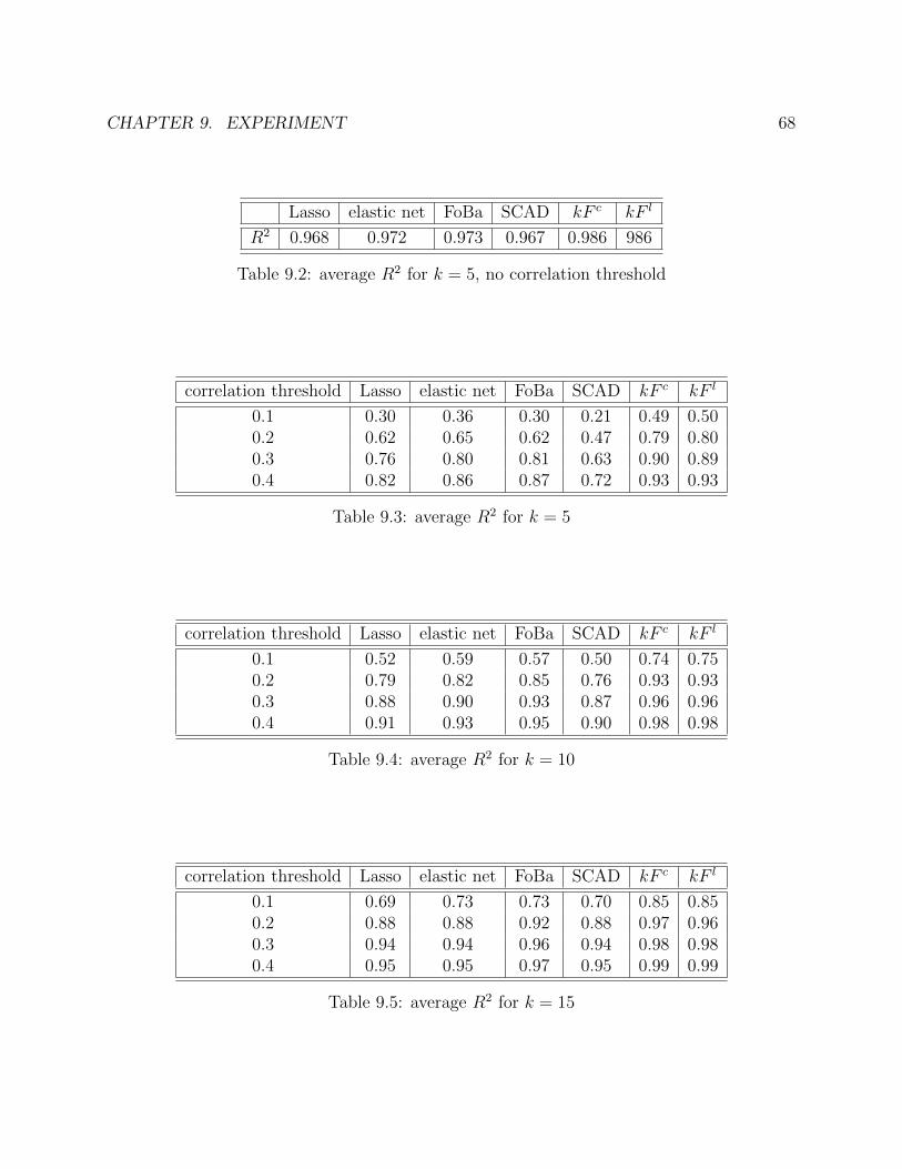
CHAPTER 9. EXPERIMENT 68
Lasso elastic net FoBa SCAD kF c kF l
R2 0.968 0.972 0.973 0.967 0.986 986
Table 9.2: average R2 for k = 5, no correlation threshold
correlation threshold Lasso elastic net FoBa SCAD kF c kF l
0.1 0.30 0.36 0.30 0.21 0.49 0.500.2 0.62 0.65 0.62 0.47 0.79 0.800.3 0.76 0.80 0.81 0.63 0.90 0.890.4 0.82 0.86 0.87 0.72 0.93 0.93
Table 9.3: average R2 for k = 5
correlation threshold Lasso elastic net FoBa SCAD kF c kF l
0.1 0.52 0.59 0.57 0.50 0.74 0.750.2 0.79 0.82 0.85 0.76 0.93 0.930.3 0.88 0.90 0.93 0.87 0.96 0.960.4 0.91 0.93 0.95 0.90 0.98 0.98
Table 9.4: average R2 for k = 10
correlation threshold Lasso elastic net FoBa SCAD kF c kF l
0.1 0.69 0.73 0.73 0.70 0.85 0.850.2 0.88 0.88 0.92 0.88 0.97 0.960.3 0.94 0.94 0.96 0.94 0.98 0.980.4 0.95 0.95 0.97 0.95 0.99 0.99
Table 9.5: average R2 for k = 15

CHAPTER 9. EXPERIMENT 69
Figure 9.5: correlation threshold v.s. average R2 for k = 5, 10, 15

CHAPTER 9. EXPERIMENT 70
Figure 9.6: k v.s. average R2 for correlation threshold = 0.1, 0.2, 0.3, 0.4

CHAPTER 10. MINIMAL CONTEXT 71
Chapter 10
Minimal Context
10.1 A Different Framework1
Suppose X = (Z, Y ), Z = (Z1, . . . , Zp)T , and we have a sample (Zi, Yi), i = 1, . . . , n, and
µ(Z) ≡ E(Y |Z) unknown. We typically approximate µ by
µN(Z) ≡N∑j=1
βjNgj(Z) + β0N
where g0 ≡ 1, g1, . . . , gN , . . . is a basis for L2(Z) and
µN(Z) ≡ arg min ‖Y −N∑j=0
βjgj(Z)‖2
For simplicity, we take µN ≡ µ with the understanding that N changes with n. Theselection of variables question informally is, “Which factors Zj are important?” The gj are,typically, functions of several variables bringing in a major complication. We consider onlythe simple case gj(Z) = Zj, N = p which illustrates the issues we raise. It is reasonableto measure effectiveness of a set S of factors by its predictive power in relation to optimalprediction. Formally, we define,
r(S) ≡ 1−‖Y − µ(Z, S)‖2 − ‖Y − µ(Z)‖2
Var(Y )
=‖µ(Z)− µ(Z, S)‖2
σ2 + ‖µ(Z)‖2
1Chapter 10.1 and 10.3 are from ”Discussion of Sara van de Geer: generic chaining andthe L1 penalty”, Peter Bickel and Mu Cai, submitted to Journal of Statistical Planning andInference.

CHAPTER 10. MINIMAL CONTEXT 72
where σ2 ≡ ‖Y − µ(Z)‖2, and
µ(Z, S) = β0 +∑βj(S)Zj : Zj ∈ S
where β0 is the intercept, and β(S) are determined by
µ(Z, S) = arg min ‖Y − β0 −p∑j=1
βjZj : Zj ∈ S‖2
Remarks: 1) βj(S) depend on S unless Zj ⊥ Zk all j 6= k. From this point of view (B2011-1)the importance of a factor depends on its context the other variables that are in the set S ofZ’s being considered as predictors.
2) It is entirely possible in the case of collinearity to have r(S1) = r(S2) = 1, S1 6= S2
and, in general, to have a class of sets Sε,m with r(S) ≥ 1− ε for S ∈ Sε,m and |S| ≤ m form(ε) sufficiently large
We define the relative contribution of Zj to the predictive power of S by
(a) c(Zj, S) =‖µ(Z, S−j)− µ(Z, S)‖2
‖µ(Z)‖2
where S−j = Zk : k ∈ S, k 6= j.This leads us to the following approach to the importance of a variable Zj in a context
S.
(i) We want the context to have high predictive power, r(S) ≥ 1− ε
(ii) We want the context as small as possible for interpretability, |S| ≤ s0
(iii) We want the contribution of Zj, c(Zj, S) to the predictive power of the context behigh.
Next we note that by orthogonality,
(b) c(Zj, S) =β2j (S)
‖µ(Z)‖2E(Zj − Π(Zj|[S−j])
)2
= (Y, Zj − Zj)2/‖µ(Z)‖2‖Zj − Zj‖2
where Π(·|L) is L2 projection onto a linear space, [S] ≡ Linear span of S, and
Zj ≡ Π(Zj|[S−j]) .
We can also write
c) c(Zj, S) =(1 +
σ2
‖µ(Z)‖2
)corr2
(Y, Zj − Zj
).

CHAPTER 10. MINIMAL CONTEXT 73
We introduce two more concepts. S is ε minimal if r(S) ≥ 1− ε and r(S−j) ≤ 1− 2ε forall j ∈ S.
Finally Zj is δ important in minimal ε context S iff c(Zj, S) ≥ 1− δ.Our goal is, having chosen δ, ε to find all (δ, ε) relevant factors, as above.If p is small we know how to solve the problem using all subsets regression. What if p is
large? We assume
A0: There is a sparse representation, i.e. For S, |S| ≤ m0 <∞ independent of p, n
E(Y − ZT (S)β(S)
)2= arg minE(Y − ZTβ)2 .
A1: For any ε minimal context, |S| ≤ s0(ε) ≤ m0.
A2: The set of all ε minimal contexts, C(ε), has
|C(ε)| ≤M0
A3: The minimal eigenvalues of all Gram matrices of minimal contexts is ≥ τ > 0.
A4: The distribution of Y is subGaussian, for all t > 0
EetY ≤ expt2λ2
2
where λ2 ≡ Var(Y )
A5: |Zj| ≤M all j = 1, . . . , p.
Essentially we are ruling out situations where good prediction is achieved by combininga large number of factors each contributing negligibly – not because we do not believe suchsituations exist but because we cannot usefully distinguish what factors are important insuch cases.
Proposition 10.1.1. If we ignore computational considerations then under A1-A5, even ifp, n → ∞ we can identify all ε minimal contexts and δ important factors within them iflog pn→ 0.
Proof. Since by (A1) the size of all ε minimum contexts is bounded by s0, it suffices to showthat we can find a consistent estimate t of the minimal prediction error t and then, among allsubset of factors of cardinality ≤ m0, find those sets with empirical predictive error ≥ (1−ε)tand then among those, identify the δ important factors. Suppose we have t. We claim thatit is then enough to show that for any S, |S| ≤ s0,
P[β(S)− β(S) ≥ ε
]≤ Ce−ε
2nγ (10.1)

CHAPTER 10. MINIMAL CONTEXT 74
for c, γ independent of s0. We can then examine all(pm
), m ≤ s0 regressions of Y on m
factors, m ≤ s0. The union sum inequality applied to (1) and the condition of the propositionensures that the minimum empirical MSE of regressions based on ≤ m0 factors converges tothe population MSE. We need only slightly refine the results of Fu and Knight (FK2000-1)for p fixed, EZ = 0. Write
Σ =1
n
n∑i=1
ZiZTi (S)− ZZT (S)
where Zi(S) ≡ Zij : j ∈ Ss0×1.
Σ(S) = EZ1ZT1 (S) .
By definition,
1
n[ZS]Y =
1
n[ZS][ZS]T β(S)
EZ1(S)Y = Σ(S)β(S)
Y ≡ (Y1, . . . , Yn)T
[ZS] ≡ [Z1(S), . . . ,Zn(S)]s0×n
[ZS] ≡ [ZS]−(Z(S), . . . , Z(S)
)By assumptions A4, A5
P[∣∣ [ZS]Y
n− EZ(S)Y
∣∣ ≥ t]≤ 2e−
t2n2M2λ2 (10.2)
sinceEet(ZijYi−EZijYi) ≤ et
2M2λ2/2
where λ2 = VarY .Also,
1
n[ZS][ZS]T = Σ(S) .
We can apply Oliveira’s (O2010-1) inequality to obtain
P[ 1
n‖
n∑i=1
(ZiZ
Ti (S)− Σ(S)
)‖ ≥ t
]≤ s0 exp− nt2
(8 + 4t)s0M2 (10.3)
since E|Zi(S)|2 ≤ s0M2.
Finally,
P[‖ZZT (S)‖2 ≥ t
]= P
[|Z|2(S) ≥ t
]≤ s0P
[|Z1| ≥
√t
s0
]≤ 2s0e
− tn
2M2s20 . (10.4)

CHAPTER 10. MINIMAL CONTEXT 75
By A3, (10.3) and (10.4),
P[‖Σ−1(S)− Σ−1(S)‖ ≥ ε
]≤ ce−nδε
2/2 (10.5)
for suitable c and δ. Then combining (10.2) and (10.5) the proposition follows given aconsistent estimate of t. However, since we know there is a sparse representation with≤ m0 factors, we can, in principle, compute µ(Z) the LSE for the regression minimizing theempirical LSE on all sets of m0 predictors. Then ‖Y − µ(Z)‖2
n gives us t. We can argue forconsistency as we did for (10.3)-(10.5).
Note that we could let s0 tend to∞ but this is of little interest. The major open questionis formulating conditions under which,
(1) σ2 (or ‖µ(Z)‖2) is consistently estimable
(2) C(ε) can be identified in less than O(pm0) operations.
We consider a data matrix (Zn×p,Yn×1) and the usual linear model
Y = Zβp×1 + e
with E(e|Z) = 0. We assume that there is a sparse representation. We seek the set of allminimal contexts C(ε). We assume we are given an algorithm `(Z, Y,m0) which returns m0
columns indices of Z, S = i1, . . . , im0 such that
β(S) = arg min‖Y − Z(S)β‖2
n : βm0×1
.
β(S), an LSE of β, will lead to an asymptoticallly sparse representation of Zβ.We sketch an algorithm for finding all minimal contexts given access to oracle βset(k)
which returns k column indices of X corresponding to k variables that have best R2 to fit Y :
βset(k) = arg min‖β‖0≤k
‖Y −Xβ‖22 (10.6)
In reality, as we do not have access to the oracle, let MC(X, Y, k) denote a generic methodwhich generates a single minimum context of size k and with it an estimate of the bestR2. This could be the Lasso (T1996-1), Elastic Net (ZH2005-1), SCAD (FL2001-1), MC+(Z2010-1), FoBa (Z2011-1), or kFoward proposed in Chapter 7.
Given MC() we construct by an iterative method AMC(X, Y, k, θr) a maximal collectionof minimal contexts of size k with R2 ≥ θr, such that no context is contained in the unionof all other contexts. The method scales as O(kN(k)|MC(k)|), where N(k) is the numberof minimum contexts, and |MC(k)| is the computation cost of MC(X, Y, k) for short.

CHAPTER 10. MINIMAL CONTEXT 76
10.2 Algorithm
Given MC(X, Y, k), consider following algorithm to recover all minimum contexts with R2 ≥θr:
FC(D)
if ∃j0 s.t.∑
iDij0 = m thenreturn j0
elsej0 ← any index s.t.
∑iDij0 6= 0
I1 ← i : Dij0 6= 0I2 ← 1, ...,m − I1
I3 ← j :∑
i∈I1 Dij 6= 0Dij ← 0 for ∀i ∈ I2 and ∀j ∈ I3
D′ ← D(I2)
L← FC(D′)return j0 ∪ L
end if
AMC(X, Y, k, θr)
J1 ←MC(X, Y, k)r ← R2 (R square) of βols(X, Y, J1)m← 1while r > θr doA← ∪mi=1JiConstruct D ∈ 0, 1m×|A| s.t. Dij = 1 if and only if jth element of A is in Ji.for s = 1 to k doLs ← FC(D)Dij ← 0 for ∀i and ∀j ∈ LsI ← Ac ∪ (A\Ls)J ←MC(XI , Y, k)r ← R2 of βols(X, Y, J)if r > θr thenm← m+ 1Jm ← Jbreak for
end ifend for
end whilereturn Jimi=1

CHAPTER 10. MINIMAL CONTEXT 77
For m = 0, 1, ... iteratively, suppose m minimum contexts Jimi=1 have been recovered, thegoal is to recover the (m+ 1)th minimum context Jm+1, assuming that there is at least onevariable of Jm+1 is outside the support of previous minimum contexts A = ∪mi=1Ji. The ideais to find a set of sets of indices C0 = Ls, with the property that Ls ∩ Ji 6= ∅ for all s andi, and for all possible Jm+1 6⊂ A, there exists Ls0 ∈ C0 s.t. Jm+1 ⊂ [p]\Ls0 . If |C0| is small,then apply MC(X[p]\Ls , Y, k) for all Ls ∈ C0 would guarantee to recover minimum contextJm+1, or we can conclude there is no more size k minimal context with R2 > θr. Since noneof Ji for i ≤ m is included in [p]\Ls for all Ls, any solution other than Jm+1 would yield asignificantly worse R2 by the definition of minimum context. Now the problem boils downto find C0 with small size efficiently. Not surprisingly, there exists such C0 with size exactlyk. One way to find it would be for s = 1, 2, ..., k, recursively find Ls s.t. Ls ∩ (∪s−1
l=1Ll) = ∅and ∑
j∈Ls
m∑i=1
I(j ∈ Ji) = m (10.7)
For details see algorithm FC(D) above.
10.3 Simulation
We simulate a multi-context toy model designed so that in the presence of large p methodsbased on screening single variables fail. This is similar to the simulation experiment inChapter 9. This type of example was suggested to us by Boaz Nadler and Ya’acov Ritov.Construct standardized predictors X ∈ Rn×p and response Y ∈ Rn as follows. DenoteXi ∈ Rn the ith column of X. Let Z1, Z2, ... be i.i.d. n dimensional standard Gaussianwith identity covariance matrix. We construct m minimum contexts of size k with commonintersection of size s, where k p and s < k. For w ∈ Rm, for each j = 1, ...,m, fori = (j − 1)(k − s) + 1, ..., j(k − s), for Y0 defined immediately later, let
Uj =
j(k−s)∑l=(j−1)(k−s)+1
Zl (10.8)
Vi = wj(Zi −ZTi Uj‖Uj‖2
2
Uj) + Y0 (10.9)
Xi =Vi√
V ar(Vi)(10.10)

CHAPTER 10. MINIMAL CONTEXT 78
Next let Xm(k−s)+1, ..., Xp be entry-wise i.i.d. standard Gaussian, and let
Y0 =
(m+1)(k−s)∑l=m(k−s)+1
Zl (10.11)
Y1 =
m(k−s)+s∑l=m(k−s)+1
Xl (10.12)
Y = SNR(Y0 + Y1) + ε (10.13)
where SNR is signal to noise ratio, ε ∈ Rn is entry-wise i.i.d standard Gaussian independentof X. We have constructed m minimum contexts of size k with a common intersection ofsize s < k, where the jth minimum context is of the form:
XJj = Xi : i ∈ Jj (10.14)
Jj = (j − 1)(k − s) + 1, ..., j(k − s) ∪ m(k − s) + 1, ...,m(k − s) + s (10.15)
w is a parameter controlling difficulty of recovery of minimum context: if Xi ∈ Jj is con-structed with associate wj, then cor(Xi, Y ) approximately scales as k−s√
(k−s+w2j )k
, i.e. the
larger wj is, the weaker correlation between Xi and Y . For small w which is relativelyeasy to recover, every method performs more or less the same. However for bigger w, cleardistinctions among methods are observed.
Next we run AMC(X, Y, k, θr) with MC(X, Y, k). Different versions of MC includeglmnet(Lasso (T1996-1) and Elastic Net (ZH2005-1)), SCAD (FL2001-1), MC+ (Z2010-1),FoBa (Z2011-1) and kForward proposed in Chapter 7. All methods are used as describedin Chapter 9 Section 9.1.
Specifically, an experiment is simulated for 4 minimum contexts each of size 6 with acommon intersection of size 2, signal to noise ratio SNR = 1, sample size n = 150 anddimension p = 1000, 2000, 3000. In this case k = 4, s = 2,m = 4. As mentioned above,w ∈ Rm is a measurement of recovery difficulty of individual minimum context. Three choicesof w are used in the simulation: w = (5, 5, 5, 5), w = (10, 10, 10, 10) and w = (15, 15, 15, 15).For Xi constructed using w, the mean and sd of cor(Xi, Y ) are reported in Table 10.1. For20 iterations, the mean and sd of number of minimum contexts(out of 4) recovered by eachmethod are reported in Table 10.2, Figure 10.1, Figure 10.2 and Figure 10.3.
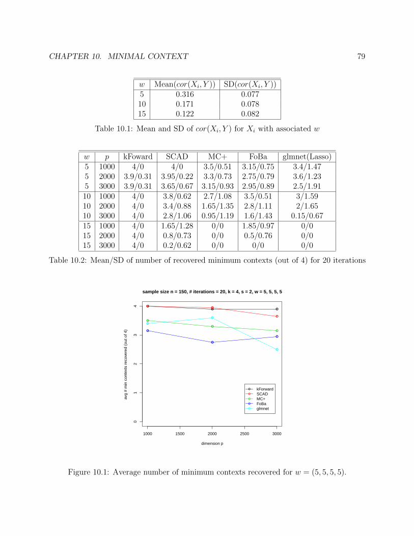
CHAPTER 10. MINIMAL CONTEXT 79
w Mean(cor(Xi, Y )) SD(cor(Xi, Y ))5 0.316 0.07710 0.171 0.07815 0.122 0.082
Table 10.1: Mean and SD of cor(Xi, Y ) for Xi with associated w
w p kFoward SCAD MC+ FoBa glmnet(Lasso)5 1000 4/0 4/0 3.5/0.51 3.15/0.75 3.4/1.475 2000 3.9/0.31 3.95/0.22 3.3/0.73 2.75/0.79 3.6/1.235 3000 3.9/0.31 3.65/0.67 3.15/0.93 2.95/0.89 2.5/1.9110 1000 4/0 3.8/0.62 2.7/1.08 3.5/0.51 3/1.5910 2000 4/0 3.4/0.88 1.65/1.35 2.8/1.11 2/1.6510 3000 4/0 2.8/1.06 0.95/1.19 1.6/1.43 0.15/0.6715 1000 4/0 1.65/1.28 0/0 1.85/0.97 0/015 2000 4/0 0.8/0.73 0/0 0.5/0.76 0/015 3000 4/0 0.2/0.62 0/0 0/0 0/0
Table 10.2: Mean/SD of number of recovered minimum contexts (out of 4) for 20 iterations
1000 1500 2000 2500 3000
01
23
4
dimension p
avg
# m
in c
onte
xts
reco
vere
d (o
ut o
f 4)
ooooo
kForwardSCADMC+FoBaglmnet
sample size n = 150, # iterations = 20, k = 4, s = 2, w = 5, 5, 5, 5
Figure 10.1: Average number of minimum contexts recovered for w = (5, 5, 5, 5).
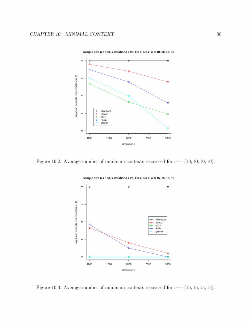
CHAPTER 10. MINIMAL CONTEXT 80
1000 1500 2000 2500 3000
01
23
4
dimension p
avg
# m
in c
onte
xts
reco
vere
d (o
ut o
f 4)
ooooo
kForwardSCADMC+FoBaglmnet
sample size n = 150, # iterations = 20, k = 4, s = 2, w = 10, 10, 10, 10
Figure 10.2: Average number of minimum contexts recovered for w = (10, 10, 10, 10).
1000 1500 2000 2500 3000
01
23
4
dimension p
avg
# m
in c
onte
xts
reco
vere
d (o
ut o
f 4)
ooooo
kForwardSCADMC+FoBaglmnet
sample size n = 150, # iterations = 20, k = 4, s = 2, w = 15, 15, 15, 15
Figure 10.3: Average number of minimum contexts recovered for w = (15, 15, 15, 15).

BIBLIOGRAPHY 81
Bibliography
BL2008a
Peter J. Bickel and Elizaveta Levina, Regularized estimation of large covariance matrices,Annals of Statistics, 2008.
BL2008b
Peter J. Bickel and Elizaveta Levina, Covariance regularization by thresholding, Annals ofStatistics, 2008.
CZZ2010
T. Tony Cai, Cun-Hui Zhang and Harrison H. Zhou, Optimal rates of convergence forcovariance matrix estimation, Annals of Statistics, 2010.
CL2011
T. Cai and W. Liu, Adaptive thresholding for sparse covariance matrix estimation, Journalof American Statistical Association, 2011.
CZ2012
T. Tony Cai and Harrison H. Zhou, Optimal rates of convergence for sparse covariancematrix estimation, Annals of Statistics, 2012.
CY2012
T. Tony Cai and Ming Yuan, Adaptive covariance matrix estimation through blockthresholding, Annals of Statistics, 2012.
EK2007
Noureddine El Karoui, Operator norm consistent estimation of large dimensional sparsecovariance matrices, Annals of Statistics, 2007.
FB2007
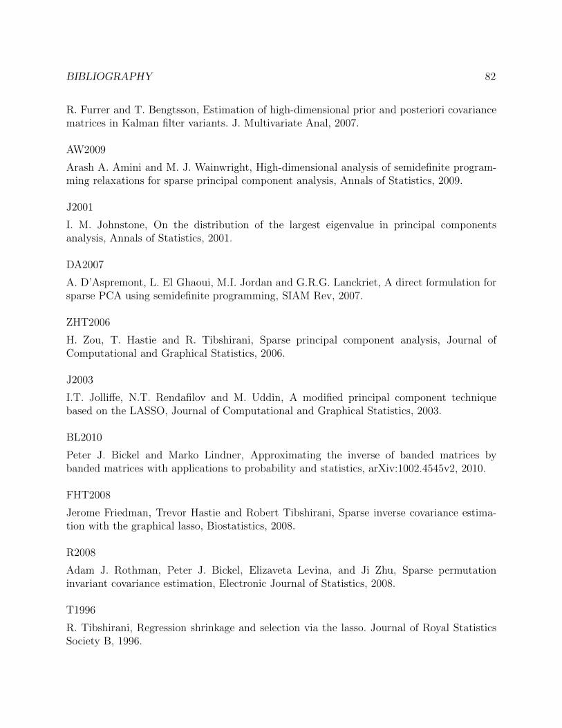
BIBLIOGRAPHY 82
R. Furrer and T. Bengtsson, Estimation of high-dimensional prior and posteriori covariancematrices in Kalman filter variants. J. Multivariate Anal, 2007.
AW2009
Arash A. Amini and M. J. Wainwright, High-dimensional analysis of semidefinite program-ming relaxations for sparse principal component analysis, Annals of Statistics, 2009.
J2001
I. M. Johnstone, On the distribution of the largest eigenvalue in principal componentsanalysis, Annals of Statistics, 2001.
DA2007
A. D’Aspremont, L. El Ghaoui, M.I. Jordan and G.R.G. Lanckriet, A direct formulation forsparse PCA using semidefinite programming, SIAM Rev, 2007.
ZHT2006
H. Zou, T. Hastie and R. Tibshirani, Sparse principal component analysis, Journal ofComputational and Graphical Statistics, 2006.
J2003
I.T. Jolliffe, N.T. Rendafilov and M. Uddin, A modified principal component techniquebased on the LASSO, Journal of Computational and Graphical Statistics, 2003.
BL2010
Peter J. Bickel and Marko Lindner, Approximating the inverse of banded matrices bybanded matrices with applications to probability and statistics, arXiv:1002.4545v2, 2010.
FHT2008
Jerome Friedman, Trevor Hastie and Robert Tibshirani, Sparse inverse covariance estima-tion with the graphical lasso, Biostatistics, 2008.
R2008
Adam J. Rothman, Peter J. Bickel, Elizaveta Levina, and Ji Zhu, Sparse permutationinvariant covariance estimation, Electronic Journal of Statistics, 2008.
T1996
R. Tibshirani, Regression shrinkage and selection via the lasso. Journal of Royal StatisticsSociety B, 1996.

BIBLIOGRAPHY 83
YZ2011
Xiaotong Yuan and Tong Zhang, Truncated Power Method for Sparse Eigenvalue Problems,arXiv:1112.2679, 2011.
Y1997
Bin Yu, Assouad, Fano, and Le Cam, Festschrift for Lucien Le Cam. D. Pollard, E.Torgersen, and G. Yang, pp. 423-435, Springer-Verla, 1997.
D1992
D.L. Donoho, I.M. Johnstone, J.C. Hoch and A.S. Stern, Maximum entropy and the nearlyblack object, Journal of the Royal Statistical Society, Series B, 1992.
CDS1998
S.S. Chen, D.L. Donoho and M.A. Saunders, Atomic Decomposition by Basis Pursuit,SIAM Journal on scientific computing, 1998.
MB2006
Nicolai Meinshausen and Peter Buhlmann, High-dimensional graphs and variable selectionwith the Lasso, Annals of Statistics, 2006.
ZY2006
Peng Zhao and Bin Yu, On Model Selection Consistency of Lasso, The Journal of MachineLearning Research, 2006.
W2006
M. Wainwright, Sharp thresholds for high-dimensional and noisy recovery of sparsity.Technical Report 708, Dept. Statistics, Univ. California, Berkeley, 2006.
CT2007
E. Candes and T. Tao, The Dantzig selector: Statistical estimation when p is much largerthan n (with discussion), Annals of Statistics, 2007.
BRT2009
Peter J. Bickel, Ya’acov Ritov and Alexandre B. Tsybakov, Simultaneous analysis of Lassoand Dantzig selector, Annals of Statistics, 2009.
ZH2005

BIBLIOGRAPHY 84
H. Zou and T. Hastie, Regularization and Variable Selection via the Elastic Net, Journal ofthe Royal Statistical Society, Series B, 2005.
Z2006
H. Zou, The Adaptive Lasso and Its Oracle Properties, Journal of the American StatisticalAssociation, 2006.
FL2001
J. Fan and R. Li, Variable selection via nonconcave penalized likelihood and it oracleproperties, Journal of American Statistical Association, 2001.
FL2002
J. Fan and R. Li, Variable Selection for Cox’s Proportional Hazards Model and FrailtyModel, Annals of Statistics, 2002.
Z2010
Cun-Hui Zhang, Nearly unbiased variable selection under minimax concave penalty, Annalsof Statistics, 2010.
Z2011
T. Zhang, Adaptive Forward-Backward Greedy Algorithm for Learning Sparse Representa-tions, IEEE Transactions on Information Theory, 2011.
B2011
Richard A. Berk, Lawrence D. Brown, Andreas Buja, Kai Zhang and Linda Zhao, ValidPost-Selection Inference, Annals of Statistics, 2011.FK2000
Wenjiang Fu and Keith Knight, Asymptotics for lasso-type estimators, Annals of Statistics,2000.
O2010
Roberto Imbuzeiro Oliveira, Concentration of the adjacency matrix and of the Laplacian inrandom graphs with independent edges, arXiv:0911.0600, 2010.J2012
Jiashun Jin, Cun-Hui Zhang and Qi Zhang, Optimality of Graphlet Screening in High Di-mensional Variable Selection, arXiv: 1204.6452, 2012.K2012

BIBLIOGRAPHY 85
Tracy Ke, Jiashun Jin and Jianqing Fan, Covariance Assited Screening and Estimation,arXiv: 1205.4645, 2012.S2011
Liangcai Shu, Aiyou Chen, Ming Xiong and Weiyi Meng, Efficient Spectral NeighborhoodBlocking for Entity Resolution, ICDE 2011.P2002
H. Pasula, B. Marthi, B. Milch, S. Russell, and I. Shpitser, Identity uncertainty and citationmatching, Advances in Neural Information Processing (NIPS), 2002.F2009
W. Fan, X. Jia, J. Li, and S. Ma, Reasoning about record matching rules, The 35th Inter-national Conference on Very Large Data Bases (VLDB), 2009.N1959
H. B. Newcombe, J. M. Kennedy, S. J. Axford, and A. P. James, Automatic linkage of vitalrecords, Science, 1959.F1969
I. Fellegi and A. Sunter, A theory for record linkage, Journal of the American StatisticalSociety, 1969.B2004
I. Bhattacharya and L. Getoor, Iterative record linkage for cleaning and integration, ACMSIGMOD Workshop on Research Issues in Data Mining and Knowledge Discovery, 2004.B2003
M. Bilenko and R. J. Mooney, Adaptive duplicate detection using learnable string similaritymeasures, SIGKDD, 2003.BG2004
I. Bhattacharya and L. Getoor, Deduplication and group detection using links, ACM SIGKD-D Workshop on Link Analysis and Group Detection, 2004.


![SummaryMap ward2 [Converted] · 2019-10-01 · MU-2 MU-6 MU-16 MU-14 MU-6 MU-2 MU-20 MU-9 MU-4 MU-13 MU-15 MU-13 MU-16 MU-18 MU-22 MU-19 MU-16 MU-27 MU-4 MU-3A MU-17 MU-13 MU-4](https://img.pdfslide.net/doc/110x75/5f5e4f591750d150e9633369/summarymap-ward2-converted-2019-10-01-mu-2-mu-6-mu-16-mu-14-mu-6-mu-2-mu-20.jpg)