Mueller Matrix Microscopy

Author: Marta Baldrıs CalmetFacultat de Fısica, Universitat de Barcelona, Diagonal 645, 08028 Barcelona, Spain.∗

Abstract:We describe a microscope that can measure simultaneously all the Mueller matrixelements of a sample with high spatial resolution. This measure is possible thanks to the dualrotating compensator method, which analyses the variation in time of the intensity at every pixelof the camera detector. This work reports the measurement principle, the instrumental details, thecalibration, and some applications of the microscope.

I. INTRODUCTION

The Mueller matrix is a useful mathematical tool tocharacterize the optical properties of a medium at cer-tain wavelength. A wide range of optical properties ofthe material can be calculated from the Mueller matrix.The optical characterization of materials and media withMueller matrices is used in many fields of science, forexample in the study biological tissues [1], for remotesensing in the ocean [2], for polarimetry of anisotropicchiral media [3], or in liquid crystals studies [4].

The objective of this work is to build up a microscopethat can measure the Mueller matrix of a sample withhigh spatial resolution. The antecedent of this Muellermatrix microscope (MMM) is the Polarized Light Micro-scope (PLM). The PLM is typically used to study the lin-ear birefringence of optically anisotropic samples and, forexample, it has a lot of applications in textile industries(as an indicator of the stretching degree) or in geology(for mineral identification). The Mueller Matrix Micro-scope represents a generalization of the PLM and it canbe also used for all these applications. The main differ-ence between both microscopes is that in PLM the resultsof linear birefringence are based on the visual analysis ofthe polarization colors, while in a MMM all the opticalproperties (linear birefringence, lineal dichroism, circu-lar birefringence, etc) are measured quantitatively andsimultaneously.

There are several experimental approaches to measurea complete Mueller matrix, for example, the four pho-toelastic modulators technique [5] or the dual rotatingcompensators approach [6]. This last technique is com-patible with the uses of a camera as a detector, becausethe camera detectors (CCD or CMOS) are relatively slowand cannot be used with photoelastic modulators (whichwork in the KHz range). Camera detectors are suitableto work with much lower frequencies than those allowedby the dual rotating compensators approach, so this tech-nique is suitable for imaging.

In our MMM we apply this last technique, so that po-larization of light is modulated by two compensators thatrotate at different frequencies. The sample is placed be-tween these two compensators, and a camera is contin-uously collecting images while the compensators rotate.

∗Electronic address: mbaldrca8@ub.edu

From the analysis of the variation of this intensity withtime, the elements of the Mueller Matrix of this samplecan be recovered.

In this article we will show the measurement princi-ple of the Mueller Matrix Microscope, we will explainthe calibration process, and finally we will present someexamples of different measurements.

II. THEORY AND INSTRUMENTATION

A. Mathematical development

There are two ways of describing a completely polar-ized light: with Jones vectors and Jones matrices, whichare related with amplitudes of electric fields, and withStokes vectors and Mueller matrices, which are associ-ated with intensities. In our case, we have consideredthis second method. The Stokes vector of light is givenby:

S =

IQUV

=

〈|Ex|2 + |Ey|2〉〈|Ex|2 − |Ey|2〉〈E∗

xEy + ExE∗y〉

i〈E∗xEy + ExE

∗y〉

, (1)

where I, Q, U, V are the Stokes parameters, and Ex, Eyare the amplitudes of electric field.

The changes of a Stokes vector by an optical system ora medium can be given as:

Sout = MSin (2)

where M is a Mueller matrix of a medium and it expresseshow the polarization of light is modified. The Muellermatrix is a 4x4 matrix which contains 16 real parametersand it is written as:

M =

m00 m01 m02 m03

m10 m11 m12 m13

m20 m21 m22 m23

m30 m31 m32 m33

(3)

To measure the Mueller matrix of a sample with the dualrotating compensators technique, we have to build an op-tical train that includes two polarizers and two rotatingcompensators as proposed by Azzam [7]. The intensitymeasured at the detector can be found from the multi-plication of the Mueller matrices of each element of theoptical system.

I = (1000) ·PL90 ·WP2 ·M ·WP1 ·PL0 · (1000)T (4)

Mueller matrix Microscopy Marta Baldrıs Calmet

PL corresponds to the Mueller matrix of the polarizers,where the subscript is the angle of orientation. WP in-dicates the Mueller matrix of the compensators, and thesubscripts indicate whether it is the first or the second.

We call the polarizer and the compensator placed be-fore the sample (PL0 and WP1) polarization state gener-ator (PSG), whereas the compensator and the polarizerthat are placed after the sample right before detector(WP2 and PL90) are called polarization state analyser(PSA).

The orientation of both polarizers is arbitrary as longas it is well known. In our case, the polarizers are crossedto obtain more contrast during the alignment.

The Mueller matrices of our crossed polarizers are:

PL0 =

1 1 0 01 1 0 00 0 0 00 0 0 0

PL90 =

1 −1 0 0−1 1 0 00 0 0 00 0 0 0

(5)

Notice that they are assumed to be ideal and do not haveany dependence.

The Mueller matrix of a compensator depends on theretardation that it causes to polarized light, and on theorientation of its optic axis. During the measurement,the compensator is continuously rotating so its orienta-tion is changing with time at a certain angular velocity.The Mueller matrix of the compensator is given by:

WPi = R(−θi) ·

1 0 0 00 1 0 00 0 cos(δi) sin(δi)0 0 −sin(δi) cos(δi)

·R(θi) (6)

R(θi) =

1 0 0 00 cos(2θi) sin(2θi) 00 −sin(2θi) cos(2θi) 00 0 0 1

(7)

where δ is the retardation of the compensator, θ is theorientation of the fast axis, and R(θ) is the rotation ma-trix.

The parameter δ depends on the wavelength of lightused during the measurement, and its value is determinedduring the calibration.

In our instrument, θi varies with time due to the ro-tating compensator setup. The value of θi with time isgiven by:

θi(t) = ωit+ φi (8)

where ω is the angular speed, which is different toeach compensator, and it can be adjusted before themeasurement with the motor controller. φ is the phase(the orientation of the compensator at time zero).

If we multiply the matrices in Eq. (2) we will find theintensity expression, that can be parameterized as:

I(θ1, θ2) =

4∑i,j=1

cij(θ1, θ2)mij (9)

where mij are the Mueller matrix elements of thesample, cij are the coefficients that parametrizes thecontribution of the device elements, and it includes allthe orientation information of the compensator.

From (9) we must determine the value of every coeffi-cient cij . If we have calculated these coefficents we willfind:

c00 = 1

c01 = C22θ1 + Cδ1S

22θ1

c02 = C2θ1S2θ1 − Cδ1C2θ1S2θ1

c03 = Sδ1S2θ1

c10 = −(C22θ2 − Cδ2S

22θ2)

c11 = −(C22θ2 + Cδ2S

22θ2)(C2

2θ1 + Cδ11S22θ1)

c12 = −(C22θ2 + Cδ2S

22θ2)(C2θ1S2θ1 − Cδ1C2θ1S2θ1)

c13 = −Sδ1S2θ1

(C2

2θ2 + Cδ2S22θ2

)c20 = Cδ2C2θ2S2θ2 − C2θ2S2θ2

c21 = −(C2

2θ1 + Cδ1S22θ1

)(C2θ2S2θ2 − Cδ2C2θ2S2θ2)

c22 = − (C2θ2S2θ2 − Cδ2C2θ2S2θ2) (C2θ1S2θ1 − Cδ1C2θ1S2θ1)

c23 = −Sδ1S2θ1 (C2θ2S2θ2 − Cδ2C2θ2S2θ2)

c30 = Sδ2S2θ2

c31 = Sδ2S2θ2

(C2

2θ1 + Cδ1S22θ1

)c32 = Sδ2S2θ2 (C2θ1S2θ1 − Cδ1C2θ1S2θ1)

c33 = Sδ2Sδ1S2θ2S2θ1

We have used a short notation, for example:cos(2θ1) ≡ C2θ1 i sin(δ1) ≡ Sδ1

The intensity detected by the camera pixel to pixel overtime and the parameters cij are the known variables ofthe system, while mij are the unknown. These equationsdepend on the retardation of the compensators (δ1 andδ2) and on the orientation (θ1 and θ2). As it is shown inEq. 8, θ1 and θ2 depend on the angular speed and thephase.

B. Device

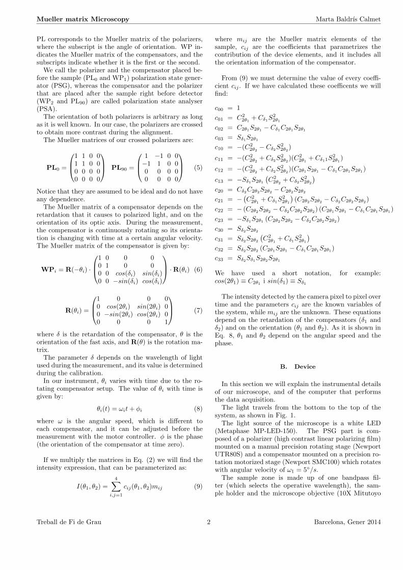
In this section we will explain the instrumental detailsof our microscope, and of the computer that performsthe data acquisition.

The light travels from the bottom to the top of thesystem, as shown in Fig. 1.

The light source of the microscope is a white LED(Metaphase MP-LED-150). The PSG part is com-posed of a polarizer (high contrast linear polarizing film)mounted on a manual precision rotating stage (NewportUTR80S) and a compensator mounted on a precision ro-tation motorized stage (Newport SMC100) which rotateswith angular velocity of ω1 = 5◦/s.

The sample zone is made up of one bandpass fil-ter (which selects the operative wavelength), the sam-ple holder and the microscope objective (10X Mitutoyo

Treball de Fi de Grau 2 Barcelona, Gener 2014

Mueller matrix Microscopy Marta Baldrıs Calmet

Plan Apo Infinity-Corrected Long WD, or 50X MitutoyoPlan Apo HR Infinity-Corrected), which can easily bereplaced.

The PSA part is made up of the same elements asPSG and its compensator rotates with angular velocityω2 = 25◦/s. The top of the microscope is made up of acamera (uEye UI-3370CP) and its telecentric objective .It is important to mention that the optical system hasbeen built on an antivibration table, to avoid externalvibrations.

The camera has a resolution of 752×480 (0.36 MP) andis sensitive to all the visible range and a small part of UV.We have chosen the LED light source because it features ahigh intensity in all the camera range, so we can select thewavelength of study using narrow interference bandpassfilters.

The camera and the two motors (controlled withSingle-Axis Controller, SMC 100) are connected to a per-sonal computer, using the USB 2.0 bus. With a softwaremade by Labview 2012 we are able to move the motors,collect all data and calculate the Mueller matrix values.

Figure 1: Schematic of the microscope.

III. MEASUREMENT PRINCIPLE ANDCALIBRATION

A. Measurement principle

The two basic parameters that control the acquisitionare the frame rate of the camera (that is always kept at50 fps) and the number of acquired images N. We haveto adjust N to a value high enough to allow the slowestcompensator to do a complete turn (typically this meansthat N is at least 3600 in our microscope).

Equation (9) expresses the intensity I(θ1, θ2) as a sum-mation extended to all the elements of the matrix as amultiplication of the coefficients cij(θ1, θ2) with the ele-ments of the Mueller matrix mij . The variables θ1 andθ2 are change over time, so the intensity changes too.

We have defined a new A vector, which includes allthe 16 elements of the Mueller matrix sample, so we canexpress this equation as:

I(t) = CT (t)A (10)

where I is an scalar number, and CT is a vector that in-cludes all the system coefficients found in the last section,where the superscript ”T” denotes transposition.

If we take N measurements, we can include the inten-sity analysis in time restating this equation as a multi-plication of a matrix by a vector:

I = CTA

And now I is a vector with N elements, CT is N × 16matrix, and A is the vector containing all the Muellermatrix elements.

Using the algebra properties we can isolate vector Amultiplying C on each side of the equation. With thefollowing result:

CI = CCTA (11)

we can express A like:

A = RI where R = CT · (CCT )−1 (12)

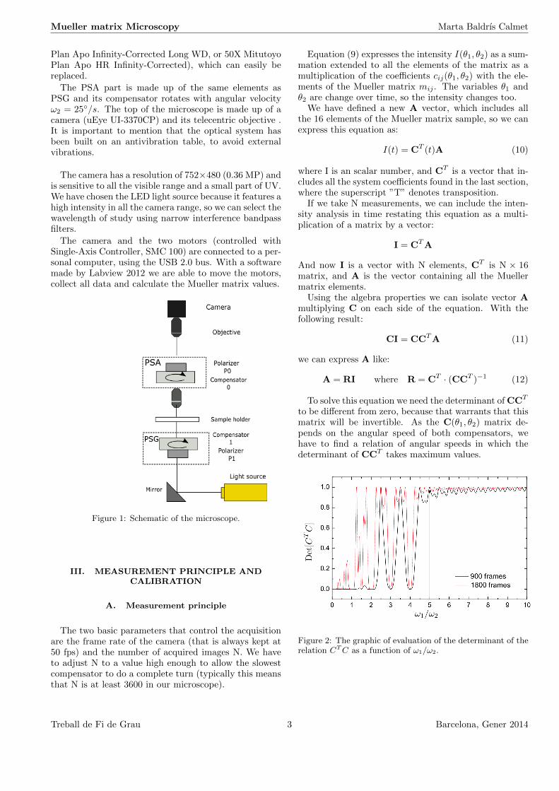
To solve this equation we need the determinant of CCT

to be different from zero, because that warrants that thismatrix will be invertible. As the C(θ1, θ2) matrix de-pends on the angular speed of both compensators, wehave to find a relation of angular speeds in which thedeterminant of CCT takes maximum values.

Figure 2: The graphic of evaluation of the determinant of therelation CTC as a function of ω1/ω2.

Treball de Fi de Grau 3 Barcelona, Gener 2014

Mueller matrix Microscopy Marta Baldrıs Calmet

In Fig. 2 we represent the value of the determinantdepending on the different relations of two motors ve-locities. As we can see, there are several relations ofrotations speed that are suitable (when the determinanttakes maximum values).

In our microscope system we have chosen the relationof 1:5 for the motors velocity. This is the reason why thePSG motor rotates at 5◦/s and the PSA motors does it at25◦/s. Once we have determined suitable values for theangular speeds, the measurement can start. Every pixelwill give us a different reading of the intensity so we haveto repeat the calculation of Mueller matrix elements forevery pixel (in our case 360000 times). We will exposethe results as a 4×4 matrix of images. The value of everyMueller matrix element is codified in a color scale.

B. Precision and errors

Before calibration, we are going to determine the pre-cision of the angular phase due to the velocity of themotors. This angular precision can be found by:

∆φ = ω ·∆t (13)

where ω is the angular speed, and ∆t is the inverse ofthe frame rate. We obtain the following precision in thedetermination of the phase.

∆φ1 = 5 · 1

50= 0.1◦

∆φ2 = 25 · 1

50= 0.5◦

So, the angular precision for the PSG motor that movesω1 = 5◦/s is 0.1◦, and for the PSA motor that movesω2 = 25◦/s it is 0.5◦.

In Ref.[8] we can see the propagated error associatedwith each element of the Mueller matrix for small errorsin the determination of phases φ1 and φ2 and retardationδ1 and δ2 values.

C. Calibration

In the calibration we are going to determine the valuesof retardation of the compensators, δ1 and δ2, and theoffset phase φ1 and φ2.

The value of the offset phases has to be constant inall the wavelength range, while retardation values canchange slightly depending on the wavelength of measure-ments.

To calibrate our microscope we have taken into accountthe fact that in the absence of sample the Mueller matrixthat we should measured is the identity matrix. To avoidany distortion made by the objective we have removed itduring the calibration. To start the calibration we makea measurement and adjust these four parameters until weobtain the identity matrix. For every wavelength that wewant to study we have to repeat the calibration.

Filter (nm) δ2 (o) δ1 (o) φ2 offset (o) φ1 offset (o)

400 71.5 133

430 88 115

532 91.7 89 148.9 ±0.5 -103.5 ±0.1

545* 90.9 86.5

610 84.7 74.5

* means broadband

Table I: Retardance and phase parameters of the PSA andPSG determined during calibration.

Table I shows the calibration parameters for our micro-scope at different wavelengths. Once we have adjustedthese parameters, if we want to measure the Mueller ma-trix of any sample we will introduce the objective. Theobjectives we use are strain free but, they may still intro-duce some minor changes in the polarization that we havenot considered in our calculation. To correct its pertur-bations we are going to measure a ”blank measurement”without sample, and we can extract the objective effectsas a matrix Mobj . We must always measure this matrixwhenever we replace the objective, modify the aligmentof the system or change the wavelength of measurement.

To correct the objective effect in our sample measure-ments we are going to carry out the following calculation:

M = M−1obj ·Msample (14)

and we are going to repeat this operation for every pixel.

IV. MEASURES

The calculus to find the optical properties from aMueller matrix are complex and it is explain in theRef.[8]. In this section we will show some of the mea-sures made using the Mueller matrix microscope. We willexpose three examples, a measurement of linear birefrin-gence in textile polymer, a measurement of the Muellermatrix of a mosquito wing and a measurement of theMueller matrix of the benzil polycrystalline.

A. Mosquito wing

Figure 3: Mosquito wing measured at 610 nm.

Treball de Fi de Grau 4 Barcelona, Gener 2014

Mueller matrix Microscopy Marta Baldrıs Calmet

In this figure we shows the Mueller matrix of amosquito wing. We can see that the little feathersof a portion of mosquito wing present high opticalanisotropies, as linear birefringence and linear dichroism.

B. Textile polyester

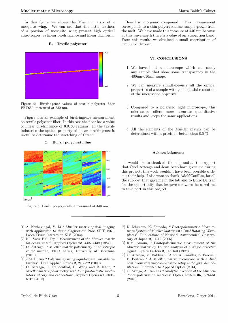
Figure 4: Birefringence values of textile polyester fiberPET650, measured at 532 nm.

Figure 4 is an example of birefringence measurementon textile polyester fiber. In this case the fiber has a valueof linear birefringence of 0.0135 radians. In the textileindustries the optical property of linear birefringence isuseful to determine the stretching of thread.

C. Benzil polycrystalline

Figure 5: Benzil polycrystalline measured at 440 nm.

Benzil is a organic compound. This measurementcorresponds to a thin polycrystalline sample grown fromthe melt. We have made this measure at 440 nm becauseat this wavelength there is a edge of an absorption band.From this results we obtained a small contribution ofcircular dichroism.

VI. CONCLUSIONS

1. We have built a microscope which can studyany sample that show some transparency in the400nm-650nm range.

2. We can measure simultaneously all the opticalproperties of a sample with good spatial resolutionof the microscope objective.

3. Compared to a polarized light microscope, thismicroscope offers more accurate quantitativeresults and keeps the same applications.

4. All the elements of the Mueller matrix can bedetermined with a precision better than 0.5 %.

Acknowledgments

I would like to thank all the help and all the supportthat Oriol Arteaga and Joan Anto have given me duringthis project, this work wouldn’t have been possible with-out their help. I also want to thank Adolf Canillas, for allthe support that gave me in the lab and to Enric Beltranfor the opportunity that he gave me when he asked meto take part in this project.

[1] A. Nezhuvingal, Y. Li “ Mueller matrix optical imagingwith application to tissue diagnostics” Proc. SPIE 4961,Laser-Tissue Interaction XIV (2003).

[2] KJ. Voss, E.S. Fry “ Measurement of the Mueller matrixfor ocean water”, Applied Optics 23, 4427-4439 (1984).

[3] O. Arteaga, “ Mueller matrix polarimetry of anisotropicchiral media”, Ph.D. thesis, University of Barcelona(2010).

[4] J.M. Bueno “ Polarimetry using liquid-crystal variable re-tarders” Pure Applied Optics 2, 216-222 (2000).

[5] O. Arteaga, J. Freudenthal, B. Wang and B. Kahr, “Mueller matrix polarimetry with four photoelastic modu-lators: theory and calibration”, Applied Optics 51, 6805-6817 (2012).

[6] K. Ichimoto, K. Shinoda, “ Photopolarimetric Measure-ment System of Mueller Matrix with Dual Rotating Wave-plates”, Publications of National Astronomical Observa-tory of Japan 9, 11-19 (2006).

[7] R.M. Azzam, “ Photopolarimetric measurement of theMueller matrix by Fourier analysis of a single detectedsignal” Optics Letters 2, 148-150 (1998).

[8] O. Arteaga, M. Baldrıs, J. Anto, A. Canillas, E. Pascual,E. Bertran “ A Mueller matrix microscope with a dualcontinuous rotating compensator setup and digital demod-ulation” Submitted to Applied Optics (2014).

[9] O. Artega, A. Canillas “ Analytic inversion of the Mueller-Jones polarization matrices” Optics Letters 35, 559-561(2010).

Treball de Fi de Grau 5 Barcelona, Gener 2014