Multi-BP expert system for fault diagnosis of powersystem

Engineering Applications of Artificial Intelligence 26 (2013) 937–944

Contents lists available at SciVerse ScienceDirect

Engineering Applications of Artificial Intelligence

0952-19

http://d

n Corr

E-m

journal homepage: www.elsevier.com/locate/engappai

Multi-BP expert system for fault diagnosis of power system

Deyin Ma, Yanchun Liang, Xiaoshe Zhao, Renchu Guan, Xiaohu Shi n

College of Computer Science and Technology, Key Laboratory of Symbol Computation and Knowledge Engineering of the Ministry of Education, Jilin University, Changchun, China

a r t i c l e i n f o

Article history:

Received 7 March 2012

Accepted 28 March 2012Available online 18 April 2012

Keywords:

Power system

Expert system

Multi-BP networks

76/$ - see front matter & 2012 Elsevier Ltd. A

x.doi.org/10.1016/j.engappai.2012.03.017

esponding author.

ail address: [email protected] (X. Shi).

a b s t r a c t

Fault diagnosis and assessment is a crucial and difficult problem for power system. Back propagation

neural network expert system (BPES) is an often used method in fault diagnosis. However, with the

layer numbers increasing, BPES becomes time consuming and even hard to converge. To solve this

problem, we divide the whole networks into many sub-BP groups within a short depth and then

propose a novel Multi-BP expert system (MBPES) based method for power system fault diagnosis. We

use two real power system data sets to test the effectiveness of MBPES. Experimental results show that

MBPES obtains higher accuracy than two commonly used methods.

& 2012 Elsevier Ltd. All rights reserved.

1. Introduction

In modern times, power system becomes larger and morecomplex than before. With its fast development, higher demandfor the sustainability and stability of power system is of greatrequirement. However, some common faults in power systemhave never been resolved very well and are still hindering thestability of power system, such as transmission fault, networkdistribution fault, power variable fault (Mizutani et al., 2007).Sometimes, even only one fault could destroy the equipments inpower system, and might affect the whole power system. An evenworse damage could cause conflagration and casualties, andleading to a huge pecuniary loss. Therefore, it is of greatsignificance to do researches for preventing those faults frompower system. And fault diagnosis is a powerful tool to guaranteethe safety and reliability of power system.

In power system, transformer is a kind of major equipmentand plays an important role in power transmission. It can raisevoltage so that power can be transported to the user with lessloss. On the other hand, the transformer can reduce power intodifferent voltage levels, which can satisfy variety needs of users.Because of its complex structure and function, transformer istending to cause fault. Unfortunately, transformer fault is verydifficult to predict. Moreover, if some accidents take place intransformer, the whole system has no choice but to stop to checkand maintain the equipments. Therefore, it is believed thatkeeping the transformer running in perfect situation plays a keyrole in power system diagnosis (Lin and Zeng, 2009). High voltagecircuit breaker (over 3 kV) is another important element in powersystem. It has two main functions, namely controlling and

ll rights reserved.

protecting. Firstly, it decides when and which parts of the powersystem should be started or stopped according to the require-ments; secondly, when some errors occur in power networks orequipments, the high voltage circuit breaker will quickly break offthe error parts from power system, so that other parts can workwithout influence. In other words, high voltage circuit breaker isable to control the normal current in power lines, and to deal withthe overload current, short-circuit current and other abnormalcurrent within a limited time. When a mistake happens in highvoltage circuit breaker, it will usually expand to other parts of thepower system and finally lead to a worse accident.

There are some classical artificial intelligence technologieshave been used in power system fault diagnosis, for example:the expert system (Ma et al., 2010), artificial neural networks(El-madany et al., 2011; Zhu et al., 2006; Huang et al., 2002;Karthikeyan et al., 2005), decision tree theory (Qu and Gao, 2008)etc. In recent years, some new theories have been applied in thisfield, such as data mining (Athanasopoulou and Chatziathanasiou,2009), fuzzy set theory (Lee et al., 2000; Zhang et al., 2010), roughset theory (Li and Wang, 2010, Li et al., 2011), petri-network(Yang et al., 2004), support vector machine (Eristi and Demir,2010), multi-agent systems (Zaki et al., 2007), and so on. Li andLiu had performed a comprehensive review of the above-men-tioned methods (Li and Liu, 2010). They pointed out that there aresome problems in the existing intelligent fault diagnosis expertsystem theology, such as the difficulty for knowledge gaining andmanaging, low on-line usage of fault diagnosis, high error rate,poor efficiency of inference process, and so on. Back propagationneural network (BPNN) expert system is an often used method infault diagnosis. In real applications, BPNN usually has manylayers. However, the training time of BPNN will grow exponen-tially with the layer number increasing. While more seriousproblem is that it is difficult to converge when BPNN has a largenumber of layers. Another problem is that the diagnostic accuracy

www.elsevier.com/locate/engappai

www.elsevier.com/locate/engappai

dx.doi.org/10.1016/j.engappai.2012.03.017



mailto:[email protected]


D. Ma et al. / Engineering Applications of Artificial Intelligence 26 (2013) 937–944938

of BPNN is still not satisfied. To solve those problems, we proposea so called multi-BP expert system (MBPES) method. In MBPES,the whole BPNN networks are divided into many sub-BP groupswithin a short depth, saying about 5 layers. In this manner, theconsumed training time is greatly reduced and it is easy toachieve the convergence of the training process.

In the experiments, we firstly compare the performance ofBPNN with different number layers according to a XOR problem.Numerical results show that when the layer number is more than6, BPNN is very time consumed and even hard to converge. To testthe effectiveness of the proposed MBPES method, it is applied totwo real power system data sets, namely that the transformerdata set and high voltage circuit breaker data set. Experimentalresults show that MBPES is very efficient, and it is more accuratethan two other compared methods.

2. Back propagation expert system

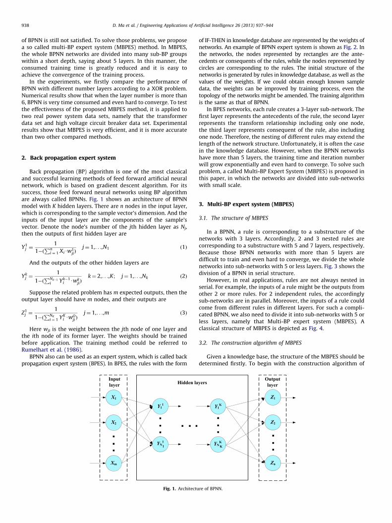
Back propagation (BP) algorithm is one of the most classicaland successful learning methods of feed forward artificial neuralnetwork, which is based on gradient descent algorithm. For itssuccess, those feed forward neural networks using BP algorithmare always called BPNNs. Fig. 1 shows an architecture of BPNNmodel with K hidden layers. There are n nodes in the input layer,which is corresponding to the sample vector’s dimension. And theinputs of the input layer are the components of the sample’svector. Denote the node’s number of the jth hidden layer as Nj,then the outputs of first hidden layer are

Y1j ¼

1

1�ðPn

i ¼ 1 XiUw1jiÞ

j¼ 1,. . .,N1 ð1Þ

And the outputs of the other hidden layers are

Ykj ¼

1

1�ðPNk�1

i Yk�1i Uwk

jiÞk¼ 2,. . .,K; j¼ 1,. . .,Nk ð2Þ

Suppose the related problem has m expected outputs, then theoutput layer should have m nodes, and their outputs are

Z1j ¼

1

1�ðPNK

i ¼ 1 YKi UwO

ji Þj¼ 1,. . .,m ð3Þ

Here wji is the weight between the jth node of one layer andthe ith node of its former layer. The weights should be trainedbefore application. The training method could be referred toRumelhart et al. (1986).

BPNN also can be used as an expert system, which is called backpropagation expert system (BPES). In BPES, the rules with the form

X1

X2

Inputlayer

Y11

Hidden la

Xm

YN11

Fig. 1. Architectu

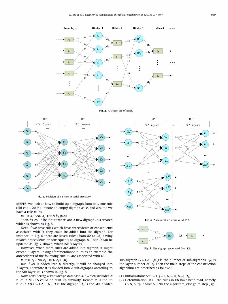
of IF-THEN in knowledge database are represented by the weights ofnetworks. An example of BPNN expert system is shown as Fig. 2. Inthe networks, the nodes represented by rectangles are the ante-cedents or consequents of the rules, while the nodes represented bycircles are corresponding to the rules. The initial structure of thenetworks is generated by rules in knowledge database, as well as thevalues of the weights. If we could obtain enough known sampledata, the weights can be improved by training process, even thetopology of the networks might be amended. The training algorithmis the same as that of BPNN.

In BPES networks, each rule creates a 3-layer sub-network. Thefirst layer represents the antecedents of the rule, the second layerrepresents the transform relationship including only one node,the third layer represents consequent of the rule, also includingone node. Therefore, the nesting of different rules may extend thelength of the network structure. Unfortunately, it is often the casein the knowledge database. However, when the BPNN networkshave more than 5 layers, the training time and iteration numberwill grow exponentially and even hard to converge. To solve suchproblem, a called Multi-BP Expert System (MBPES) is proposed inthis paper, in which the networks are divided into sub-networkswith small scale.

3. Multi-BP expert system (MBPES)

3.1. The structure of MBPES

In a BPNN, a rule is corresponding to a substructure of thenetworks with 3 layers. Accordingly, 2 and 3 nested rules arecorresponding to a substructure with 5 and 7 layers, respectively.Because those BPNN networks with more than 5 layers aredifficult to train and even hard to converge, we divide the wholenetworks into sub-networks with 5 or less layers. Fig. 3 shows thedivision of a BPNN in serial structure.

However, in real applications, rules are not always nested inserial. For example, the inputs of a rule might be the outputs fromother 2 or more rules. For 2 independent rules, the accordinglysub-networks are in parallel. Moreover, the inputs of a rule couldcome from different rules in different layers. For such a compli-cated BPNN, we also need to divide it into sub-networks with 5 orless layers, namely that Multi-BP expert system (MBPES). Aclassical structure of MBPES is depicted as Fig. 4.

3.2. The construction algorithm of MBPES

Given a knowledge base, the structure of the MBPES should bedetermined firstly. To begin with the construction algorithm of

Outputlayeryers

Y1K

YNKK

Z1

Z2

Zn

re of BPNN.

R11

a1

a2

b1

1.0

1.0

cf1 Rk1

c1

cf1

a3

a4

an

R12

R13

R14

R1i

b2

bm

Rk2

Rkj

cp

1.0

1.0

1.0

1.01.0

1.0

cf2

cf3

cf4

cfi

cf2

cfj

1.0

1.0

1.0

1.0

Input layer Hidden 1 ...

...

1.0

...

...

...

...

...

Hidden 2 Hidden 3 Hidden 4

Fig. 2. Architecture of BPES.

PBPB

X1

X4

Xn

X5

X3

X2 Y1

Z1

Y3

Y2

Ym

Z2

Z3

Z4

Zk...

...

...

layers5≤ layers5≤

Fig. 3. Division of a BPNN in serial structure.

X11

Y1

Y2

Ym

... ...

...Z1

1

Z21

ZK11

...

PBPB

......

...

......

X21

XN11

X1G

X2G

XNGG

Z1G

Z2G

ZKGG

layers5 layers5< <

Fig. 4. A classical structure of MBPES.

R1

a1

a2

b1

1.0

1.00.8

Fig. 5. The digraph generated from R1.

D. Ma et al. / Engineering Applications of Artificial Intelligence 26 (2013) 937–944 939

MBPES, we look at how to build up a digraph from only one rule(Shi et al., 2006). Denote an empty digraph as F, and assume wehave a rule R1 as

R1: IF a1 AND a2 THEN b1 (0.8)Then, R1 could be input into F, and a new digraph D is created

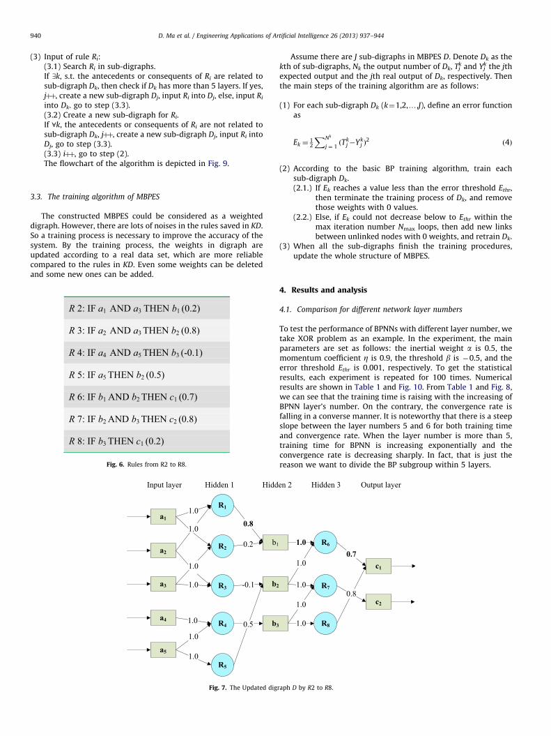
which is shown as Fig. 5.Next, if we have rules which have antecedents or consequents

associated with D, they could be added into the digraph. Forinstance, in Fig. 6 there are seven rules (from R2 to R8) havingrelated antecedents or consequents to digraph D. Then D can beupdated as Fig. 7 shown, which has 5 layers.

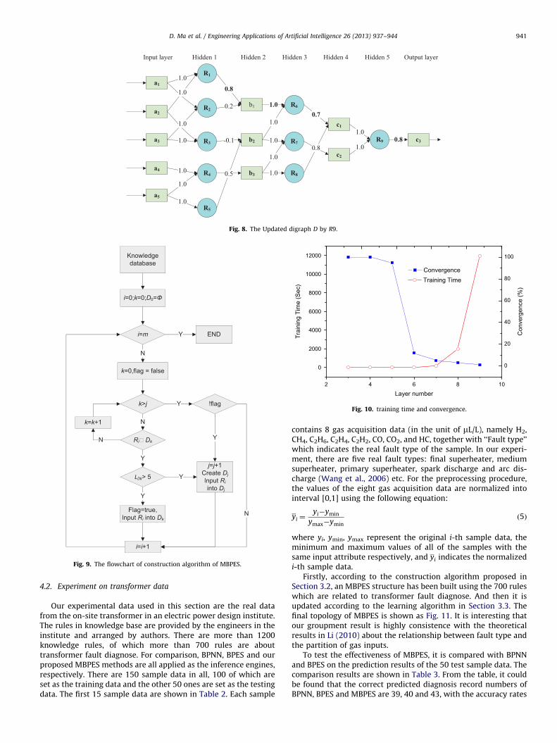
However, when more rules are added into digraph, it mightexceed 6 layers. Taking aforementioned rules as an example, theantecedents of the following rule R9 are associated with D:

R 9: IF c1 AND c2 THEN c3 (0.8).But if R9 is added into D directly, it will be changed into

7 layers. Therefore it is divided into 2 sub-digraphs according tothe 5th layer. It is shown in Fig. 8.

Now considering a knowledge database KD which includes N

rules, a MBPES could be built up similarly. Denote Ri is the ithrule in KD (i¼1,2,y,N), D is the digraph, Dk is the kth divided

sub-digraph (k¼1,2,y,j), j is the number of sub-digraphs, LDk isthe layer number of Dk. Then the main steps of the constructionalgorithm are described as follows:

(1)
Initialization: Set i¼1, j¼1, D1¼F, D¼{ D1}; (2) Determination: If all the rules in KD have been read, namely
i4N, output MBPES, END the algorithm, else go to step (3);


(3)
Input of rule Ri:(3.1) Search Ri in sub-digraphs.If (k, s.t. the antecedents or consequents of Ri are related tosub-digraph Dk, then check if Dk has more than 5 layers. If yes,jþþ, create a new sub-digraph Dj, input Ri into Dj, else, input Ri
into Dk. go to step (3.3).(3.2) Create a new sub-digraph for Ri.If 8k, the antecedents or consequents of Ri are not related tosub-digraph Dk, jþþ, create a new sub-digraph Dj, input Ri intoDj, go to step (3.3).(3.3) iþþ, go to step (2).The flowchart of the algorithm is depicted in Fig. 9.

3.3. The training algorithm of MBPES

The constructed MBPES could be considered as a weighteddigraph. However, there are lots of noises in the rules saved in KD.So a training process is necessary to improve the accuracy of thesystem. By the training process, the weights in digraph areupdated according to a real data set, which are more reliablecompared to the rules in KD. Even some weights can be deletedand some new ones can be added.

Fig. 6. Rules from R2 to R8.

R1

a1

a2

b1

1.00.8

a3

a4

a5

R2

R3

R4

R5

b2

b3

1.0

1.0

1.0

1.0

1.0

1.0

0.2

-0.1

Input layer Hidden 1 Hidd

0.5

Fig. 7. The Updated dig

Assume there are J sub-digraphs in MBPES D. Denote Dk as thekth of sub-digraphs, Nk the output number of Dk, Tk

j and Ykj the jth

expected output and the jth real output of Dk, respectively. Thenthe main steps of the training algorithm are as follows:

(1)

en 2

raph

For each sub-digraph Dk (k¼1,2,y,J), define an error functionas

Ek ¼12

XNk

j ¼ 1ðTk

j�Ykj Þ

2ð4Þ

(2)
According to the basic BP training algorithm, train eachsub-digraph Dk.(2.1.) If Ek reaches a value less than the error threshold Ethr,
then terminate the training process of Dk, and removethose weights with 0 values.

(2.2.) Else, if Ek could not decrease below to Ethr within themax iteration number Nmax loops, then add new linksbetween unlinked nodes with 0 weights, and retrain Dk.

1.0

1.0

1.0

1.0

H

1.0

D by R2

(3)
When all the sub-digraphs finish the training procedures,update the whole structure of MBPES.
4. Results and analysis

4.1. Comparison for different network layer numbers

To test the performance of BPNNs with different layer number, wetake XOR problem as an example. In the experiment, the mainparameters are set as follows: the inertial weight a is 0.5, themomentum coefficient Z is 0.9, the threshold b is �0.5, and theerror threshold Ethr is 0.001, respectively. To get the statisticalresults, each experiment is repeated for 100 times. Numericalresults are shown in Table 1 and Fig. 10. From Table 1 and Fig. 8,we can see that the training time is raising with the increasing ofBPNN layer’s number. On the contrary, the convergence rate isfalling in a converse manner. It is noteworthy that there is a steepslope between the layer numbers 5 and 6 for both training timeand convergence rate. When the layer number is more than 5,training time for BPNN is increasing exponentially and theconvergence rate is decreasing sharply. In fact, that is just thereason we want to divide the BP subgroup within 5 layers.

R6

c1

0.7

R7

R8

c2

0.8

idden 3 Output layer

to R8.

R1

a1

a2

b1

1.00.8

1.0 R6

c1

0.7

a3

a4

a5

R2

R3

R4

R5

b2

b3

R7

R8

c2

1.0

1.0

1.0

1.0

1.0

1.0

0.2

-0.1

0.5

0.81.0

1.0

1.0

Input layer Hidden 1 Hidden 2 Hidden 3 Output layer

1.0

R9 c30.81.0

1.0

Hidden 4 Hidden 5

Fig. 8. The Updated digraph D by R9.

i k D

i m

k

k j

Ri Dk

Ri Dk

i i

j jDjRiDj

k k

Fig. 9. The flowchart of construction algorithm of MBPES.

2

0

2000

4000

6000

8000

10000

12000

Con

verg

ence

(%)

Trai

ning

Tim

e (S

ec)

Layer number

Training Time

0

20

40

60

80

100

Convergence

10864

Fig. 10. training time and convergence.


4.2. Experiment on transformer data

Our experimental data used in this section are the real datafrom the on-site transformer in an electric power design institute.The rules in knowledge base are provided by the engineers in theinstitute and arranged by authors. There are more than 1200knowledge rules, of which more than 700 rules are abouttransformer fault diagnose. For comparison, BPNN, BPES and ourproposed MBPES methods are all applied as the inference engines,respectively. There are 150 sample data in all, 100 of which areset as the training data and the other 50 ones are set as the testingdata. The first 15 sample data are shown in Table 2. Each sample

contains 8 gas acquisition data (in the unit of mL/L), namely H2,CH4, C2H6, C2H4, C2H2, CO, CO2, and HC, together with ‘‘Fault type’’which indicates the real fault type of the sample. In our experi-ment, there are five real fault types: final superheater, mediumsuperheater, primary superheater, spark discharge and arc dis-charge (Wang et al., 2006) etc. For the preprocessing procedure,the values of the eight gas acquisition data are normalized intointerval [0,1] using the following equation:

yi ¼yi�ymin

ymax�ymin

ð5Þ

where yi, ymin, ymax represent the original i-th sample data, theminimum and maximum values of all of the samples with thesame input attribute respectively, and yi indicates the normalizedi-th sample data.

Firstly, according to the construction algorithm proposed inSection 3.2, an MBPES structure has been built using the 700 ruleswhich are related to transformer fault diagnose. And then it isupdated according to the learning algorithm in Section 3.3. Thefinal topology of MBPES is shown as Fig. 11. It is interesting thatour groupment result is highly consistence with the theoreticalresults in Li (2010) about the relationship between fault type andthe partition of gas inputs.

To test the effectiveness of MBPES, it is compared with BPNNand BPES on the prediction results of the 50 test sample data. Thecomparison results are shown in Table 3. From the table, it couldbe found that the correct predicted diagnosis record numbers ofBPNN, BPES and MBPES are 39, 40 and 43, with the accuracy rates

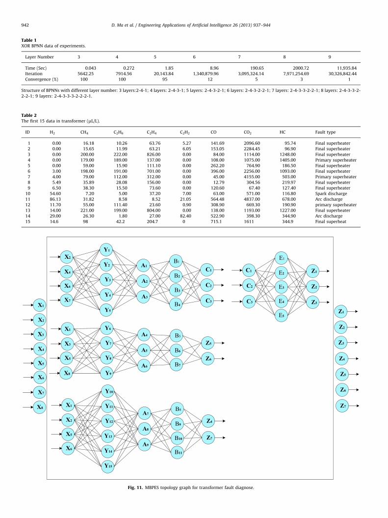
Table 2The first 15 data in transformer (mL/L).

ID H2 CH4 C2H6 C2H4 C2H2 CO CO2 HC Fault type

1 0.00 16.18 10.26 63.76 5.27 141.69 2096.60 95.74 Final superheater



4 0.00 179.00 189.00 137.00 0.00 108.00 1075.00 1405.00 Primary superheater



7 4.00 79.00 112.00 312.00 0.00 45.00 4155.00 503.00 Primary superheater



10 54.60 7.20 5.00 37.20 7.00 63.00 571.00 116.80 Spark discharge

11 86.13 31.82 8.58 8.52 21.05 564.48 4837.00 678.00 Arc discharge

12 11.70 55.00 111.40 23.60 0.90 308.90 669.30 190.90 primary superheater


14 29.00 26.30 1.80 27.00 82.40 522.90 398.30 344.90 Arc discharge

15 14.6 98 42.2 204.7 0 715.1 1611 344.9 Final superheat

Table 1XOR BPNN data of experiments.

Layer Number 3 4 5 6 7 8 9

Time (Sec) 0.043 0.272 1.85 8.96 190.65 2000.72 11,935.84

Iteration 5642.25 7914.56 20,143.84 1,340,879.96 3,095,324.14 7,971,254.69 30,326,842.44

Convergence (%) 100 100 95 12 5 3 1

Structure of BPNNs with different layer number: 3 layers:2-4-1; 4 layers: 2-4-3-1; 5 layers: 2-4-3-2-1; 6 layers: 2-4-3-2-2-1; 7 layers: 2-4-3-3-2-2-1; 8 layers: 2-4-3-3-2-

2-2-1; 9 layers: 2-4-3-3-3-2-2-2-1.

Y1

Y2

Y3

Y4

Y5

X2

X4

X6

X7

C2

C3

C1A1

A2

A3

B1

B2

B3

B4

Z2

Z3

Z1

E1

E2

E3

E4

E5

Y10

Y11

Y12

X1

X2

X5

X6

Z7

B8

B9

B10

B11

Y6

Y7

Y8

Y9

X1

X3

Z6

Z5

A4

A5

A6

B5

B6

B7

Z4

X5

X8

X3

X4

X5

X6

X1

X2

X7

X8

Z2

Z3

Z1

Z7

Z4

Z6

Z5

C2

C3

C1

Y13

Y14

Y15

A7

A8

A9

Fig. 11. MBPES topology graph for transformer fault diagnose.


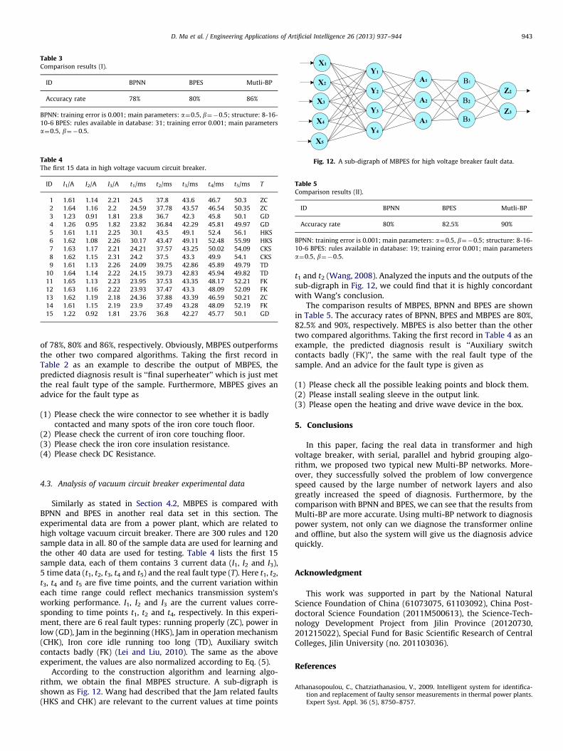
Table 3Comparison results (I).

ID BPNN BPES Mutli-BP

Accuracy rate 78% 80% 86%

BPNN: training error is 0.001; main parameters: a¼0.5, b¼�0.5; structure: 8-16-

10-6 BPES: rules available in database: 31; training error 0.001; main parameters

a¼0.5, b¼�0.5.

Table 4The first 15 data in high voltage vacuum circuit breaker.

ID I1/A I2/A I3/A t1/ms t2/ms t3/ms t4/ms t5/ms T

1 1.61 1.14 2.21 24.5 37.8 43.6 46.7 50.3 ZC

2 1.64 1.16 2.2 24.59 37.78 43.57 46.54 50.35 ZC

3 1.23 0.91 1.81 23.8 36.7 42.3 45.8 50.1 GD

4 1.26 0.95 1.82 23.82 36.84 42.29 45.81 49.97 GD

5 1.61 1.11 2.25 30.1 43.5 49.1 52.4 56.1 HKS

6 1.62 1.08 2.26 30.17 43.47 49.11 52.48 55.99 HKS

7 1.63 1.17 2.21 24.21 37.57 43.25 50.02 54.09 CKS

8 1.62 1.15 2.31 24.2 37.5 43.3 49.9 54.1 CKS

9 1.61 1.13 2.26 24.09 39.75 42.86 45.89 49.79 TD

10 1.64 1.14 2.22 24.15 39.73 42.83 45.94 49.82 TD

11 1.65 1.13 2.23 23.95 37.53 43.35 48.17 52.21 FK

12 1.63 1.16 2.22 23.93 37.47 43.3 48.09 52.09 FK

13 1.62 1.19 2.18 24.36 37.88 43.39 46.59 50.21 ZC

14 1.61 1.15 2.19 23.9 37.49 43.28 48.09 52.19 FK

15 1.22 0.92 1.81 23.76 36.8 42.27 45.77 50.1 GD

Y1

Y2

Y3

Y4

X1

X2

Z3

Z2

A1

A2

A3

B1

B2

B3

X3

X4

X5

Fig. 12. A sub-digraph of MBPES for high voltage breaker fault data.

Table 5Comparison results (II).

ID BPNN BPES Mutli-BP

Accuracy rate 80% 82.5% 90%

BPNN: training error is 0.001; main parameters: a¼0.5, b¼�0.5; structure: 8-16-

10-6 BPES: rules available in database: 19; training error 0.001; main parameters

a¼0.5, b¼�0.5.


of 78%, 80% and 86%, respectively. Obviously, MBPES outperformsthe other two compared algorithms. Taking the first record inTable 2 as an example to describe the output of MBPES, thepredicted diagnosis result is ‘‘final superheater’’ which is just metthe real fault type of the sample. Furthermore, MBPES gives anadvice for the fault type as

(1)
Please check the wire connector to see whether it is badlycontacted and many spots of the iron core touch floor.
(2)
Please check the current of iron core touching floor. (3) Please check the iron core insulation resistance. (4) Please check DC Resistance.
4.3. Analysis of vacuum circuit breaker experimental data

Similarly as stated in Section 4.2, MBPES is compared withBPNN and BPES in another real data set in this section. Theexperimental data are from a power plant, which are related tohigh voltage vacuum circuit breaker. There are 300 rules and 120sample data in all. 80 of the sample data are used for learning andthe other 40 data are used for testing. Table 4 lists the first 15sample data, each of them contains 3 current data (I1, I2 and I3),5 time data (t1, t2, t3, t4 and t5) and the real fault type (T). Here t1, t2,t3, t4 and t5 are five time points, and the current variation withineach time range could reflect mechanics transmission system’sworking performance. I1, I2 and I3 are the current values corre-sponding to time points t1, t2 and t4, respectively. In this experi-ment, there are 6 real fault types: running properly (ZC), power inlow (GD), Jam in the beginning (HKS), Jam in operation mechanism(CHK), Iron core idle running too long (TD), Auxiliary switchcontacts badly (FK) (Lei and Liu, 2010). The same as the aboveexperiment, the values are also normalized according to Eq. (5).

According to the construction algorithm and learning algo-rithm, we obtain the final MBPES structure. A sub-digraph isshown as Fig. 12. Wang had described that the Jam related faults(HKS and CHK) are relevant to the current values at time points

t1 and t2 (Wang, 2008). Analyzed the inputs and the outputs of thesub-digraph in Fig. 12, we could find that it is highly concordantwith Wang’s conclusion.

The comparison results of MBPES, BPNN and BPES are shownin Table 5. The accuracy rates of BPNN, BPES and MBPES are 80%,82.5% and 90%, respectively. MBPES is also better than the othertwo compared algorithms. Taking the first record in Table 4 as anexample, the predicted diagnosis result is ‘‘Auxiliary switchcontacts badly (FK)’’, the same with the real fault type of thesample. And an advice for the fault type is given as

(1)
Please check all the possible leaking points and block them. (2) Please install sealing sleeve in the output link. (3) Please open the heating and drive wave device in the box.
5. Conclusions

In this paper, facing the real data in transformer and highvoltage breaker, with serial, parallel and hybrid grouping algo-rithm, we proposed two typical new Multi-BP networks. More-over, they successfully solved the problem of low convergencespeed caused by the large number of network layers and alsogreatly increased the speed of diagnosis. Furthermore, by thecomparison with BPNN and BPES, we can see that the results fromMulti-BP are more accurate. Using multi-BP network to diagnosispower system, not only can we diagnose the transformer onlineand offline, but also the system will give us the diagnosis advicequickly.

Acknowledgment

This work was supported in part by the National NaturalScience Foundation of China (61073075, 61103092), China Post-doctoral Science Foundation (2011M500613), the Science-Tech-nology Development Project from Jilin Province (20120730,201215022), Special Fund for Basic Scientific Research of CentralColleges, Jilin University (no. 201103036).

References

Athanasopoulou, C., Chatziathanasiou, V., 2009. Intelligent system for identifica-tion and replacement of faulty sensor measurements in thermal power plants.Expert Syst. Appl. 36 (5), 8750–8757.


El-madany, H.T., Fahmy, F.H., El-Rahman, N.M.A., Dorrah, H.T., 2011. Spacecraftpower system controller based on neural network. Acta Astronaut. 69 (7–8),650–657.

Eristi, H., Demir, Y., 2010. A new algorithm for automatic classification of powerquality events based on wavelet transform and SVM. Expert Syst. Appl. 37 (6),4094–4102.

Huang, Y.C., Yang, H.T., Huang, K.Y., 2002. Abductive network model-baseddiagnosis system for power transformer incipient fault detection. IEE Proc.Gener. Transm. Distrib. 149 (3), 326–330.

Karthikeyan, B., Gopal, S., Vimala, M., 2005. Conception of complex probabilisticneural network system for classification of partial discharge patterns usingmultifarious inputs. Expert Syst. Appl. 29, 953–963.

Lee, H.J., Park, D.Y., Ahn, B.S., Park, Y.M., Park, J.K., Venkata, S.S., 2000. A fuzzyexpert system for the integrated fault diagnosis. IEEE Trans. Power Del. 15 (2),833–838.

Lei, H.Y., Liu, J.G., 2010. Common fault and disposal methods of vacuum circuitbreaker. Econ. Res. Guide 12, 205–254.

Li, C., 2010. Research of Power Transformer Fault Diagnosis System. ShanghaiUniversity of Electric Power 6–8.

Li, J.R., Wang, Q.H., 2010. A rough set based data mining approach for house ofquality analysis. Int. J. Prod. Res. 48 (7), 2095–2107.

Li, Q., Li, Z.B., Zhang, Q., 2011. Research of power transformer fault diagnosissystem based on rough sets and Bayesian networks. Adv. Mater. Res. 320,524–529.

Li, Z.H., Liu, M.K., 2010. Review of intelligence fault diagnosis in power system.Electr. Eng. 8, 21–24.

Lin, Y.X., Zeng, Q.J., 2009. Development of on-line monitoring system for highvoltage vacuum circuit breaker. Electron. Des. Eng. 17 (12), 21–23.

Ma, D.Y., Sun, C., Li, Z.H.X., Guan, R.C., Liang, Y.C., 2010. Uncertain management inrule-based power system using object-oriented design. In: Proceedings of the3rd International Conference on Power Electronics and Intelligent Transporta-tion System (PEITS 2010), 363–366.

Mizutani, Y., Takahashi, T., Ito, T., 2007. Lifetime evaluation method for poletransformer based on transient temperature analysis. IEEE Trans. PowerEnergy 127 (5), 653–658.

Qu, Z.Y., Gao, Y.F., Nie, X., 2008. Network fault diagnoses expert system modelbased on decision tree. Comput. Eng. 34 (22), 215–217.

Rumelhart, D.E., Hinton, G.E., Williams, R.J., 1986. Learning representations byback-propagating errors. Nature 323 (6088), 533–536.

Shi, Y., Qiu, T., Chen, B.Z., 2006. Fault analysis using process signed directed graphmodel. Chem. Ind. Eng. Prog. 25 (12), 1484–1488.

Wang, J., Liu, J.X., Wu, L.Z., 2006. Fault forecast of the transformer using newtheory of grey system. In: Proceedings of the International Conference onElectricity Distribution (CICED 2006), 20, 340–345.

Wang, N., 2008. Study on Fault Diagnosis of High Voltage Circuit Breaker Based onNeural Network Expert System. Henan University 37–40.

Yang, B.S., Jeong, S.K., Oh, Y.M., Tan, A.C., 2004. Case-based reasoning system withPetri nets for induction motor fault diagnosis. Expert Syst. Appl. 27 (2),301–311.

Zaki, O., Brown, K., Fletcher, J., Lane, D., 2007. Detecting faults in heterogeneousand dynamic systems using DSP and an agent-based architecture. Eng. Appl.Artif. Intell. 20 (8), 1112–1124.

Zhang, L.L., Li, P., Wang, T.T., Wang, H., 2010. Research of fault diagnosis based onfuzzy neutral network to power transformer. Ind. Instrum. Autom. 5, 3–5.

Zhu, Y.L., Huo, L.M., Lu, J.L., 2006. Bayesian networks-based approach for powersystems fault diagnosis. IEEE Trans. Power Del. 21 (2), 634–639.

Documents

Multi-BP expert system for fault diagnosis of powersystem