Embed Size (px)
Citation preview

Report No. CDOT-2008-8 Final Report MULTI-CRITERIA WETLANDS MAPPING USING AN INTEGRATED PIXEL-BASED AND OBJECT-BASED CLASSIFICATION APPROACH Chengmin Hsu and Lynn Johnson
September 2008 COLORADO DEPARTMENT OF TRANSPORTATION
DTD APPLIED RESEARCH AND INNOVATION BRANCH

The contents of this report reflect the views of the authors, who are responsible for the facts and accuracy of the data presented herein. The contents do not necessarily reflect the official views of the Colorado Department of Transportation or the Federal Highway Administration. This report does not constitute a standard, specification, or regulation.

Technical Report Documentation Page 1. Report No. CDOT-2008-8
2. Government Accession No.
3. Recipient's Catalog No. 5. Report Date September 2008
4. Title and Subtitle MULTI-CRITERIA WETLANDS MAPPING USING AN INTEGRATED PIXEL-BASED AND OBJECT-BASED CLASSIFICATION APPROACH
6. Performing Organization Code
7. Author(s) Chengmin Hsu and Lynn Johnson
8. Performing Organization Report No. CDOT-2008-8
10. Work Unit No. (TRAIS)
9. Performing Organization Name and Address University of Colorado Denver Department of Civil Engineering, CB 113 1200 Larimer Street Denver, CO 80217
11. Contract or Grant No.
13. Type of Report and Period Covered Final
12. Sponsoring Agency Name and Address Colorado Department of Transportation – Environmental Programs Branch 4201 E. Arkansas Ave. Denver, CO 80222 14. Sponsoring Agency Code
15. Supplementary Notes
16. Abstract The Colorado Department of Transportation (CDOT) has the challenging task of protecting the environment while developing and maintaining the best transportation systems and services possible for the citizens of Colorado. Among these tasks, a wetland inventory database is a key component required to meet the environmental protection mandate. The subject research project is directed to developing a semi-automated method to identify and classify inland wetlands in the northern Front Range area of Colorado. A goal of the project is to produce a database that accurately records wetland locations based on the classification system that is commonly used by many organization and institutions. The methodology is based on satellite imagery, high resolution aerial photos, and digital elevation model data in conjunction with field global positioning system data collections. Satellite imagery being used includes moderate resolution LANDSAT 7 ETM+, Terra ASTER, and EO-1 Hyperion/ALI. The aerial photography is from the National Agriculture Imagery Program and is mainly used for validation and sample collection purposes. The EO-1 imagery has high spectral resolution and is used to develop a wetlands spectrum signature library which is then used to observe the correlations between EO-1 and LANDSAT 7 and ASTER image bands. The image processing approach being applied uses both pixel-based and object-based classification techniques; the object-based technique accounts for the pattern of neighboring pixels and wetland boundary shapes. The variables generated for object-based classification algorithm are extracted from multi-spectral imagery and include image texture, wetland shapes, greenness, wetness, brightness, normalized difference vegetation index, principal components, stream networks, biological soil crust index, and land thermal fluctuation. In the final stage, these variables are incorporated into a hierarchical rule creation for facilitating the wetland classification operation. To complete the tasks, the software used include ArcGIS®, ENVI®, DEFINIENS® Professional. Results of the research indicate a high correspondence with wetlands mapped by field biologists and identification of additional wetlands not previously recognized.
17. Keywords USACE Wetlands Delineation Manual, wetland inventory databases, remote sensing, geographic information systems (GIS), global positioning systems (GPS), land use change, hydrological analysis
18. Distribution Statement No restrictions. This document is available to the public through the National Technical Information Service, Springfield, VA 22161
19. Security Classif. (of this report) None
20. Security Classif. (of this page) None
21. No. of Pages 48
22. Price
Form DOT F 1700.7 (8-72) Reproduction of completed page authorized
MULTI-CRITERIA WETLANDS MAPPING USING AN INTEGRATED PIXEL-BASED AND
OBJECT-BASED CLASSIFICATION APPROACH
by
Chengmin Hsu1, Lynn Johnson2
1Graduate Research Assistant, Civil Engineering 2Professor, Civil Engineering
University of Colorado Denver 1200 Larimer Street, P.O. Box 173364
Denver, CO 80217
Report No. CDOT-2008-8
Sponsored by the Colorado Department of Transportation
In Cooperation with the U.S. Department of Transportation Federal Highway Administration
September 2008

EXECUTIVE SUMMARY One of the major issues when attempting to conduct environmental assessments in
Colorado and elsewhere is the lack of information on wetlands. Functionally, wetlands
serve a critical role in benefiting the state's water resources by providing flood and erosion
control, water quality maintenance, and habitat and other ecosystem functions. But
wetlands are vanishing rapidly. Over the past two centuries, approximately 40% to 60%
(0.4-1.2 million ha; 1-3 million ac) of the original wetland areas of Colorado has been lost
(Dahl 1990, Wilen 1995). The subject research project is directed to developing a semi-
automated method to identify and classify inland wetlands in the northern Front Range
area of Colorado. A goal of the project is to develop an effective wetland mapping
methodology so that a database that accurately records wetland locations can be created.
The methodology is based on satellite imagery, high resolution aerial photos and digital
elevation model data in conjunction with field global positioning system data collections.
Satellite imagery used includes moderate resolution LANDSAT 7 ETM+, Terra ASTER,
and EO-1 Hyperion/ALI. The aerial photography is from the National Agriculture
Imagery Program. The EO-1 imagery has high spectral resolution and is used to develop a
wetlands spectrum signature library which is then used to establish correlations between
EO-1 and LANDSAT 7 and ASTER image bands. The image processing approach being
applied uses both pixel-based and object-based classification techniques; the object-based
technique accounts for the pattern of neighboring pixels (i.e. context) and wetland
boundary shapes. The variables generated for object-based classification algorithm are
extracted from multi-spectral imagery and include image texture, wetland shapes,
greenness, wetness, brightness, normalized difference vegetation index, principal
components, stream networks, biological soil crust index, and land thermal fluctuation.
Software used in the process includes ArcGIS®, ENVI®, and DEFINIENS® Professional
remote sensing software. Results of the research indicate a high correspondence with
wetlands mapped by field biologists and identification of additional wetlands not
previously recognized. The results of this research are expected to be supportive to
transportation planning by the Colorado Department of Transportation.

TABLE OF CONTENTS 1. Introduction ……………………………………………………………………………1
1.1. The Importance of Wetland Information ……………………………….……1 1.2. Regulatory Background …………………………………………………..….1 1.3. Objectives ……………………………………………………………………2 1.4. Incorporation of Object-Based Classification Algorithm ………………........3
2. Wetland Definition and Parameters ………………………………………….………..4 2.1. Parameters of Wetland Delineation of USACE …………………….…..........4 2.2. Wetland Types Adopted for Classification…………………………….…......6
3. Methods …………………………………………………………………….……….....8 3.1. Study Area and Image Acquisition ……………………………………..……8
3.2. Field Survey ……………………………………………………….………..10 3.3 Data Preparation ………………………………………………….………....12
3.3.1. Geo-Referencing ……………………………………………………..12 3.3.2. Gram-Schmidt Spectral Sharpening………………………….……....12 3.3.3. Transferring Digital Number to Reflectance ……………….……..…14
3.4. Vegetation Indices……………………………………………………..…....18 3.4.1. Kauth-Thomas Tasseled Cap Transformation …………………….…19
3.4.2. NDVI ……………………………………………………………..….21 3.5. Hydrological Analysis ……………………………………………….….….23 3.6. Unsupervised Pixel-Based Classification ……………………………..…....26 3.6.1. Minimum Noise Fraction Transformation ………………….……..…27 3.6.2. ISODATA Classification ………………………………………..….. 28 3.7. Object-Based Classification …………………………………………..….…31
3.7.1. Load and Create Project …………………………………………...…31 3.7.2. Create Image Object …………………………………………….….. 32 3.7.3. Classification …………………………………………………….…. 34
4. Results and Discussion………………………………………………………….…....37 4.1. Areas of the Wetlands Identified…………………………………….....37
4.2. KAPPA Analysis ……………………………………………….……...38 4.3. Findings and Conclusions………………………………………….…...39
5. Future Efforts ……………………………………………………………………...…40 6. Acknowledgements .……………………………………………………………..….. 42 7. References….……………….…………………………………………………….......42

LIST OF FIGURES Figure 1. Aquatic bed...........................................................................................................6 Figure 2. Marshes.................................................................................................................6 Figure 3. Wet meadows........................................................................................................7 Figure 4. Scrub/Shrub...........................................................................................................7 Figure 5. Floodplain forest ………………………………………………………………..8 Figure 6. Study area..............................................................................................................9 Figure 7. Field sample site GPS operation.........................................................................11 Figure 8. 15 Meter resolution ETM+ imagery after sharpening........................................13 Figure 9. 30 m resolution raw ETM+ imagery...................................................................13 Figure 10. LANDSAT 7 Band 4 reflectance......................................................................17 Figure 11. Generated at-satellite surface temperature of 04/16/2003 ETM+ Data............18 Figure 12. Greenness layer.................................................................................................20 Figure 13. Wetness layer…………………………………………………………….…...20 Figure 14. Brightness layer………………………………………………………....….....20 Figure 15. Reflectance of various land cover categories……………………………........21 Figure 16. The stream network ovverlaid over photograph................................................22 Figure 17. NDVI of ASTER 08/13/2003………………………………………………....22 Figure 18. NDVI of EO1 ALI 10/26/2001………………………………………………..22 Figure 19. Flow direction d8 algorithm ………………………………………...……......23 Figure 20. Flow accumulation operation concept ……………………………...………...23 Figure 21. Generated stream network……………………………………………..……...25 Figure 22. Involvement of stream layer in delineating wetlands in the neighborhood ..…26 Figure 23. MNF Band 1 of EO1 ALI data………………………………………….….…27 Figure 24. ISODATA classification on EO1 ALI 10/26/2001 data…………………..…..28 Figure 25. ISODATA classification on LANDSAT 7 04/16/2003 data……………..…...29 Figure 26. ISODATA classification on LANDSAT 7 06/16/2002 data………….….…...29 Figure 27. Weighted overlay………………………………………………………..….…30 Figure 28. Level 1 image object segmentation…………………………………….…..…33 Figure 29. Level 2 image object segmentation………………………………………...…34 Figure 30. Level 1 classification results …………………………….…………………...36 Figure 31. Comparison of individual marsh identification and its actual location ……....36 Figure 32. Photograph of one of the mapped marshes ………..………………….……....37 LIST OF TABLES Table 1. ETM+ Solar Spectrum Irridances ....................................................................... 15 Table 2. Earth-Sun Distance in Astronomical Units......................................................... 16 Table 3. ETM+ Thermal Band Calibration Constants …………………………………..18 Table 4. Error Matrix …………………………………………………………………...38

1
1. INTRODUCTION 1.1. The Importance of Wetland Information
In Colorado, wetlands are recognized as one of the most productive ecosystems by virtue
of their abundant moisture in an otherwise arid environment. In recognition of the
multitude of ecological functions and human values provided by wetlands, government
agencies are seeking to establish wetland protection programs. The Colorado Department
of Transportation (CDOT), Colorado Division of Wildlife (CDOW), US Army Corps of
Engineers (USACE), Colorado Division of Water Resources (CDWR), local
governments, and various conservation organizations are all among the institutions that
could use a wetland inventory database, so that land use decision quality can be
maintained and enhanced.
1.2. Regulatory Background
The Federal Water Pollution Control Act Amendments of 1972, amended in 1977, was
established to maintain and restore the biological, chemical, and physical integrity of the
waters of the United States. In practice, the Secretary of the Army, acting through the
Chief of Engineers, was authorized by Section 404 of the Act to issue permits for the
discharge of dredged or fill material into the waters of the United States, including
wetlands. However, to accomplish wetland regulatory functions requires knowing where
the wetlands are located. Creating a wetlands inventory database has thus become an
urgent mission for Colorado. Responding to the Clean Water Act, US Army Corps of
Engineers established the “Wetlands Delineation Manual” (USACE 1987) to provide
guidance for identification and delineation of wetlands potentially subject to regulation
under Section 404. This manual is viewed as the mandatory approach for public and
private sectors to legitimately identify wetlands. The technical guidelines for wetlands
delineation in the Corps manual do not specify a strict wetland classification system.
Rather it provides guidelines for determining whether a given area is a wetland or not for
legal regulatory purposes; such determination typically requires a field delineation of the
wetland boundary by a professional trained in wetland delineation techniques.

2
The use of remote sensing for wetlands mapping has been established by a number of
state agencies as a guide for planning purposes. A notable example in this regard is the
Wisconsin wetland inventory program developed to augment the USACE procedures. For
our work, the wetland classification system of Wisconsin Wetlands Association (WDNR
1992) was used for wetland categorization.
1.3. Objectives
The wetlands mapping research project has been motivated by requirements of the Safe,
Accountable, Flexible, and Efficient Transportation Equity Act: A Legacy for Users
(SAFETEA-LU). SAFETEA-LU authorizes the Federal surface transportation programs
for highways, highway safety and transit for the 5-year period 2005-2009. SAFETEA-LU
addresses the many challenges involved in transportation system development, such as
improving safety, reducing traffic congestion, improving efficiency in freight movement,
increasing intermodal connectivity, and protecting the environment. The provisions
include a new environmental review process for highways, transit, and multimodal
projects, with increased authority for transportation agencies such the CDOT.
The wetland identification methods developed in this research are considered highly
accurate and appropriate for transportation facilities planning purposes. The generated
wetland inventory will therefore become a valuable component for developing
cumulative impact assessments, inform transportation planning, stewardship of natural
resources, and land use allocation decisions.
The objectives of this research are to:
1. Establish a highly reliable database of wetland occurrences and distributions to
assist planning level activities.
2. Develop procedures for wetland identification using inexpensive data.
3. Create algorithms that accurately identify wetlands in a wide area.
4. Simulate the delineation method established in the USACE Wetlands Delineation
Manual by applying recent advances of geospatial technology.

3
1.4. Incorporation of Object-Based Classification Algorithm
Traditional pixel-based classification algorithms, such as parallelepiped and ISODATA
(Iterative Self-Organizing Data Analysis Technique), are carried out based on the
spectrum information of each individual pixel. With a pixel-based algorithm, the pixel is
classified according to the composition pattern of the radiation in various wavelengths
emitted from that pixel location. This type of clustering, however, doesn’t involve the
evaluation of the geographic aspects of the pixel and its contextual relationship with the
surroundings. Thus, the pixel-based classification is likely to generate many salt-and-
pepper type classifications that do not represent contiguous wetland areas. Especially
when there are not enough spectral bands in the imagery, the separation capability
between classes would be dramatically reduced by using traditional pixel-based
approaches. To overcome this deficiency, other techniques have been proposed, mainly
consisting of three categories: (a) image pre-processing, (b) contextual classification, (c)
post-classification processing, such as rule-based processing and morphological filtering.
These techniques increase classification accuracy, but their disadvantages are evident
when applied to high spatial resolution images, such as EO-1 Advanced Land Imager
imagery, IKONOS, and NAIP (National Agricultural Imagery Program) data. These
methods either require intensive computation or produce inaccurate results at the
boundaries of distinctive land cover units.
Considering the complexities of mapping wetland occurrences, the object-based
classification algorithm was developed in this project to supplement the capability of the
traditional pixel-based classification algorithms. Instead of analyzing the pixel spectrum
information for classification purposes, the mechanism of object-based classification
algorithm is able to categorize the imagery by evaluating the geometric and textural
characteristics of wetland areas as objects. Simply stated, objects are formed by grouping
contiguous pixels with homogeneous aspects of ancillary conditions, such as smoothness,
spectrum, or shape, as guided by the imagery analyst. Within objects the local spectral
variation caused by gaps, shadows, and crown textures is mitigated by the creation of the
objects at various scales. Furthermore, with objects as the minimum map units, the
object-based algorithm is able to appraise many spatial properties of wetlands; such as

4
shape, size, direction, density, distance, compactness, and texture of wetlands. Thus the
object-based approach employed in this research is not limited to the evaluation of
spectral characteristics of the hydrophytic vegetation and hydric soils, but makes
maximum use of the spatial contextual variables of wetlands, such as the wetland
distribution pattern and distances to the stream courses. This greatly enhances mapping
accuracy and completeness. The object-based classification procedures developed in this
research were executed with DEFINIENS® image processing software.
2. WETLANDS DEFINITION AND PARAMETERS
Successful identification of wetlands starts with a clear definition of wetlands. According
to USACE (1987) wetlands are defined as:
Those areas that are inundated or saturated by surface or ground water
at a frequency and duration sufficient to support, and that under normal
circumstances do support, a prevalence of vegetation typically adapted
for life in saturated soil conditions. Wetlands generally include swamps,
marshes, bogs, and similar areas.
2.1. Parameters of Wetland Delineation of USACE
The USACE (1987) wetland definition induces three mandatory environmental
characteristics for wetland detection; vegetation, soil, and hydrology. Within the manual,
these three diagnostic environmental characteristics are further characterized to provide
guidelines of this study.
• Vegetation. The widespread vegetation in wetlands is normally macrophytes
that are typically adapted to areas with hydrologic and soil environmental
conditions of saturation (USACE 1987). Hydrophytic species are the vegetation
which have the ability to grow, compete, reproduce, and/or persist in anaerobic
soil conditions. The delineation manual places emphasis on the assemblage of
plant species that are a controlling influence on the character of the plant
community rather than on indicator species. For this project characterization of
the hydrophytic plant communities in Colorado were based on data from
National Wetland Inventory website and associated field observations.

5
• Soil. The USACE Wetlands Delineation Manual (1987) set up a few criteria for
determining the presence of hydric soils. Normally, these soils possess
characteristics that are connected with anoxic soil conditions. They can be
organic soil, histic epipedons, sulfidic material, or soils of the aquic/peraquic
regime. These soils are the products of prolonged anaerobic soil conditions,
which exist when soil is inundated or saturated for sufficient duration, and will
result in chemical reduction of some soil components (e.g., iron and manganese
oxides). Soil colors and other physical characteristics thus become the indicators
of hydric soils. For the remote sensing approach, biological soil crust index
accompanied by the generated emissivity or Thermal Response number, was
used to emulate the soil identification process specified in the USACE
delineation manual.
• Hydrology. According to the USACE manual (1987), wetland identifications
should include the hydrologic characteristics that result in inundation either
permanently or periodically at mean water depths ≤ 6.6 ft. Otherwise, at some
time during the growing season of the prevalent vegetation, the soil is saturated
to the surface. Topographically, the areas of lower elevation in a floodplain or
marsh have more frequent periods of inundation and/or greater duration than
most areas at higher elevations. For plant cover factors, areas of abundant plant
cover make additional water drain more slowly and thus increase frequency and
duration of inundation or soil saturation. Conversely the transpiration rates of
the sites may give the investigated field an entirely opposite effect. The evapo-
transpiration rates may be higher in areas with abundant plant cover and reduce
the duration of soil saturation. This plant canopy factor, associated with other
indicators such as drainage patterns, drift lines, sediment deposition,
watermarks, stream gage data and flood predictions, historic records, visual
observations of saturated soils and inundation, bring a rigorous criteria for
wetland hydrological process evaluation. In this research, the use of Tasseled
Cap transformation techniques, hydrological analysis on topographic data, and
the concept of surface temperature, some of the field hydrologic indicators
mentioned above can be incorporated using remote sensing techniques.

6
2.2. Wetland Types Adopted for Classification
As summarized in the previous section, wetland types are characterized by vegetation,
soil type, and degree of saturation or water cover. According to the USACE (1987)
wetland definition, all of the three diagnostic environmental characteristics need to be
satisfied to classify an area as wetlands. In contrast the Classification of Wetlands and
Deepwater Habitats of the United States (Cowardin et al., 1979) from the US Fish and
Wildlife Service (USFWS) classify a wetland by requiring only one attribute fulfillment
among the three diagnostic attributes. Considering that some inconsistency exists
between these two systems and that the USACE wetland definition had been adopted for
this research, a more general wetland classification system was used to categorize the
wetland types found in the field. However, the corresponding wetland classes of the
Wetlands and Deepwater Habitats Classification hierarchy from the USFWS were also
contained in the texts for comparison. Some of the prominent wetland types are listed
below; these form the wetland classification system for this research.
• Aquatic Bed
Plants grow entirely on or in a water body for most of the growing season in most
years. Aquatic beds in the NFRMPO area can be found in the sheltered areas of reservoirs
or ponds that have little water movement. They generally occur in water no deeper than 6
feet. Plants include pondweed, duckweed, lotus and water-lilies. They can be classified
into the Aquatic Bed class in the Lacustrine, Palustrine, or Riverine system if the
hierarchy of the Wetlands and Deepwater Habitats Classification of the USFWS is used.
Fig. 1 Aquatic bed Fig. 2 Marshes

7
• Marshes
Marshes are characterized by emergent aquatic plants growing in permanent and
seasonal shallow water with water depths of less than 6.6 feet (2 meters). The
counterparts of Marshes in the Wetlands and Deepwater Habitats Classification hierarchy
of the USFWS is Palustrine / Emergent or Lacustrine / Littoral / Emergent. In the
NFRMPO area, the marsh size can vary from a one-quarter acre pond to a long oxbow of
a river or shallow bay of a lake. The species are dominated by cattails, bulrushes,
pickerelweed, lake sedges and/or giant bur-reed.
• Wet Meadows
Wet meadows normally have saturated soil rather than standing water. Meadows
are essentially closed wetland communities (nearly 100% vegetative cover) and often act
as a transition zone between aquatic communities and uplands. Sedges, grasses and reeds
are the governing species with the possible presence of sneezeweed, marsh milkweed,
mint and several species of aster and goldenrod. Plants
occurring in meadows include species found in other
communities, such as the annuals of seasonally flooded
basins and emergent aquatic plants of marshes. With the
USFWS Wetlands and Deepwater Habitats Classification
hierarchy, wet meadows can be categorized as
Lacustrine/ Littoral/ Emergent class or Palustrine/
Emergent class.
• Scrub/Shrub
These areas, which include bogs and alder
thickets, are characterized by woody shrubs and small
trees less than 20 feet tall such as bog birch, willow,
and dogwood. This type of wetland in the NFRMPO
area mainly exists along rivers, but does not belong to a
riverine system. Instead, Scrub/Shrub is categorized as Fig. 4 Scrub/Shrub
Fig. 3 Wet meadows

8
Palustrine/ Scrub-Shrub class according to the wetland hierarchy of the USFWS.
• Floodplain Forest
The floodplain forest has its equivalent in the USFWS wetland hierarchy:
Palustrine/ Forested. These forested floodplain complexes are characterized by trees 20
feet or more in height such as Cottonwood, Elm, Salix spp., Water Birch, and Big-tooth
Maple. Grass cover underneath the trees is an important part of this system and is a mix
of tall grass species, including
Panicum virgatum and Andropogon
gerardii. There are not many flood
plain forests in the NFRMPO area;
most of the forested floodplain
complexes exist along the Cache La
Poudre River.
3. METHODS 3.1. Study Area and Image Acquisition
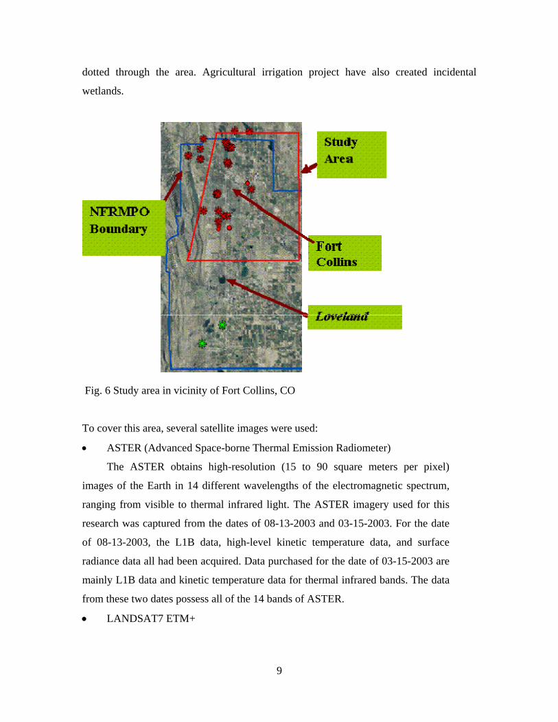
This research was conducted in the northern Front Range of Colorado covering an area
from north of Fort Collins to the north of Loveland, with I-25 crossing through the
middle from north to south (Fig. 6). The area is delimited by a trapezoid with the corners
of 105 6΄6.275 W, 40 39΄56.001 N; 104 53΄51.055 W, 40 39΄56.001 N;
104 53΄51.055 W, 40 26΄45.949 N; 105 10΄27.332 W, 40 26΄45.949 N. The study area
is about 60 miles away from Denver, Colorado. There is approximately 500 km² of area
within the project research boundary. This area consists of agriculture, urban, and
suburban zones. Most of the study area is located within the watershed of the Cache La
Poudre River. The Cache la Poudre in northern Colorado is renowned for its canal
development heritage in importing, storing and conveying water. Originating from above
the tree-line in Rocky Mountain National Park, the Cache la Poudre has become
Colorado's first and only national Wild and Scenic River. As the river and its tributaries
wander through the terrain, numerous fens, marshes, potholes, and wet meadows are
Fig. 5 Floodplain forest
9
dotted through the area. Agricultural irrigation project have also created incidental
wetlands.
Fig. 6 Study area in vicinity of Fort Collins, CO
To cover this area, several satellite images were used:
• ASTER (Advanced Space-borne Thermal Emission Radiometer)
The ASTER obtains high-resolution (15 to 90 square meters per pixel)
images of the Earth in 14 different wavelengths of the electromagnetic spectrum,
ranging from visible to thermal infrared light. The ASTER imagery used for this
research was captured from the dates of 08-13-2003 and 03-15-2003. For the date
of 08-13-2003, the L1B data, high-level kinetic temperature data, and surface
radiance data all had been acquired. Data purchased for the date of 03-15-2003 are
mainly L1B data and kinetic temperature data for thermal infrared bands. The data
from these two dates possess all of the 14 bands of ASTER.
• LANDSAT7 ETM+

10
The purchased images are the scenes captured on the dates of 06-16-2002 and
04-16-2003. The LANDSAT 7 imagery is composed of four bands of 30 m * 30 m
visible and near infrared data, two middle infrared bands, one band of thermal-
infrared data with 60 m resolution, and a 15m* 15 meter panchromatic image. The
ETM+ data was used to calculate various vegetation indices and the soil crust
index as well. The scene of 04-16-2003 was mainly used for supplementary
analysis for the spring season, when leaves hadn’t totally turned green or there
were fewer leaves present. Thus, the impacts of image signal noise from soil upon
the vegetation radiation can be observed. Comparison of the wetland hydrology,
vegetation, and soil conditions in the spring and summer increases the accuracy of
the mapping.
• EO-1 Hyperion Hyper-spectral / Advance Land Imager
To further observe the hydrophytic vegetation into the species level, hyper-
spectral data was employed to classify the vegetation species. Having only a 7.7
kilometer swath, the EO-1 Hyperion data was not used for directly delineating
wetlands. Instead, it was used for the creation of the spectrum library of the various
wetland classes and used for the comparison with the other overlapping imagery.
The obtained Hyperion hyper-spectral image has more than 220 spectral bands
(from 0.4 to 2.5 µm). The data was captured on 10-26-2001.
• NAIP (National Agriculture Imagery Program) aerial photographs
The one-meter resolution NAIP for Larimer and Weld Counties were
downloaded from the following USGS (US Geological Survey) FTP site.
ftp://rockyftp.cr.usgs.gov/ngtoc/colo_naip/
This data was mainly used for GPS data check and sample sites selection.
3.2. Field Survey
Field data collection is mandatory for successful wetland mapping. The wetland sample
sites can be either used as training sites to collect the spectrum characteristics or used as
the samples for validation purpose.

11
The sample sites of various wetlands were located using a Global Positioning System
(GPS) unit. The possible wetlands were first identified on the NAIP imagery. The field
visits were then planned accordingly. In the field, the pictures of the wetland samples
were taken and their location information was collected by using the handheld Trimble
Geo-Explorer GPS unit. In order to ensure that the accuracy of wetland locations is
within ± 2m, the recorded GPS data was post-processed using differential corrections. In
the U.S., a number of government and private agencies have made the base files for the
differential correction purpose freely available online. The data collected at the base
station is used to calculate the generated differences accompanied with the GPS satellite
signals (by finding the difference between the positions calculated from the satellite
signals and the known reference position). In the Fort Collins area there are two base
stations that continuously serve ready-to-download data every hour. Two of the collected
wetland sample sites are shown in the Fig. 7.
Fig. 7 Field samples GPS data collection

12
3.3. Data Preparation
Some basic image processing operations are required to be performed on the raw images
before obtaining the environmental indices and implementing classification processes.
These steps include geo-referencing, sharpening, and conversion to reflectance.
3.3.1. Geo-Referencing
First, since the images are collected from multiple satellite platforms, they all need to be
registered to the same projection and geographic coordinate system. This step is to
guarantee that the subsequent operations are spatially accurately executed on the layers
generated from the various satellite platforms and also to ensure that the pixel offset
between the images is constrained to the minimum. The registration accuracy is targeted
at smaller than 0.35 pixels of root mean square error (RMSE). All of the geo-referencing
operations were set up for a third-order polynomial transformation. More than 80 ground
control points were collected for each registration effort to achieve such a high accuracy
RMSE standard. In some cases, more than 100 ground control points were collected for
registering an image.
NAIP, with its high geographic accuracy, was chosen as the reference map for geo-
referencing the other satellite images. NAIP data uses UTM North America Datum 1983
as its coordinate system, thus the NAD83, UTM zone 13N was used as a common spatial
reference system for all of the images in this research. The registration processes were
executed using the ENVI® software. Most of the images were registered using the cubic
convolution algorithm in recognition that wetlands normally are located in the edge
between water bodies and uplands.
3.3.2. Gram-Schmidt Spectral Sharpening
Image fusion remote sensing techniques aim at integrating the information from multiple
images having differing spatial and spectral resolution from satellite and aerial platforms.
Given that the number and kind of satellite platforms are increasing, image fusion
techniques are increasingly important for data development by remote sensing. The
literature of image fusion shows that an optimal quality for a fused image is defined as

13
having Minimum Color Distortion (containing all the spectral property of Multi\Hyper
spectral images), Maximum Spatial Resolution (containing all the spatial property of high
resolution image) and Maximum Neutrality (the best integration of spectral and spatial
quality of input data). But this ideal situation only can be obtained theoretically (Zhou,
1998). For example, the most straightforward fusion method, Intensity-Hue-Saturation
(IHS) transformation, has been shown to have a large spectral distortion when displaying
the fusion product in color composition.
To achieve an optimal quality for the image sharpening process, the Gram-Schmidt
spectral sharpening algorithm, one of the most sophisticated methods for performing
fusion on multi-spectral and panchromatic bands, was applied in this project. This
algorithm is based on the component substitution strategy developed by Laben and
Brover (2000) and patented by Eastman Kodak. This algorithm is the method adopted by
the ENVI® package and is thus used by this research.
Basically, Gram-Schmidt spectral sharpening extracts the high frequency variation of a
high resolution image and then inserts it into the multi-spectral framework of a
corresponding low resolution image. In this algorithm, algebraic procedures operate on
images at the level of the individual pixel to proportion spectral information among the
Fig. 8 ETM+ imagery after pan-sharpening
Fig. 9 Raw ETM+ imagery (30m)

14
bands of the multi-spectral image. The replacing (high resolution) image substitutes one
of the bands of the original image and can then be assigned correct spectral brightness. A
comparison of raw image and post sharpening of LANDSAT 7 ETM+ 06/16/2002 data
by the Gram-Schmidt sharpening method is shown below. The comparison exhibits a
considerable improvement of spatial quality after sharpening, while enduring little
spectral distortion.
3.3.3. Transferring Digital Number to Reflectance
To successfully generate the vegetation and soil indices, the digital numbers of
LANDSAT 7 ETM+ need to be transferred to the reflectance. This process actually
includes two steps. The first step is to transfer the Digital Number of each band to its
radiation detected at the sensor. This process involves the calibration process of
calculation that brings the 8 bit integer data into the 32 bit floating point. The equation
used is listed below.
Lλ = "gain" * QCAL + "offset"
which is also expressed as:
Lλ = ((LMAXλ - LMINλ)/(QCALMAX-QCALMIN)) * (QCAL-
QCALMIN) + LMINλ
where:
Lλ = Spectral Radiance at the sensor aperture in watts/(meter squared * ster *
μm)
"gain" = Rescaled gain (the data product "gain" contained in the Level 1
product header or ancillary data record) in watts/(meter squared * ster
* μm)
"offset" = Rescaled bias (the data product "offset" contained in the Level 1
product header or ancillary data record ) in watts/(meter squared * ster
* μm)
QCAL = the quantized calibrated pixel value in DN
LMINλ = the spectral radiance that is scaled to QCALMIN in watts/(meter
squared * ster * μm)

15
LMAXλ = the spectral radiance that is scaled to QCALMAX in watts/(meter
squared * ster * μm)
QCALMIN = the minimum quantized calibrated pixel value (corresponding to
LMINλ) in DN
= 1 (LPGS Products)
= 0 (NLAPS Products)
QCALMAX = the maximum quantized calibrated pixel value (corresponding to
LMAXλ) in DN
= 255
All of the above variables can be obtained from the metadata accompanying the file. The
second step is to translate from surface radiation to reflectance at the sensor. The
LANDSAT scenes in this step were actually normalized for solar irradiance by
converting spectral radiance, as calculated above, to planetary reflectance or albedo. This
is a combination of surface and atmospheric reflectance of the Earth. It was computed
with the following formula:
Where:
ρp = Unitless planetary reflectance
Lλ = Spectral radiance at the sensor's aperture
d = Earth-Sun distance in astronomical units from nautical handbook or interpolated
from values listed in Table 2. In order to get a correct distance in astronomical
units, the Julian Day of the image capture date needs to be figured out.
ESUNλ = Mean solar exo-atmospheric irradiances from Table 1
θs = Solar zenith angle in degrees
Table 1 ETM+ Solar Spectral
Irradiances
Band watts/(meter squared * μm)

16
1 1969.00
2 1840.00
3 1551.00
4 1044.00
5 225.70
7 82.07
8 1368.00
The Julian Day / Calendar Day Conversion information can be found from the related
page provided by NASA Goddard Space Flight Center.
http://rapidfire.sci.gsfc.nasa.gov/faq/calendar.html
Table 2 Earth-Sun Distance in Astronomical Units
The generated LANDSAT band-4 reflectance of a portion of the study site based on the
above formula is displayed in the figure 10.

17
After transferring Digital Number of ETM+ Band 6 digital number to radiance as the
process described above, the ETM+ Band 6 imagery can also be converted from spectral
radiance to a more physically useful variable. This is done under an assumption of unity
emissivity and using pre-launch calibration constants listed in the Table below. The
effective at-satellite temperatures of the viewed Earth-atmosphere system in Fort Collins
area on the date of 04/16/2003 is displayed below. The conversion formula used in this
research is:
Where:
T = Effective at-satellite temperature in Kelvin
K2 = Calibration constant 2 from Table below
K1 = Calibration constant 1 from Table below
L = Spectral radiance in watts/ (meter squared * ster * μm)
Fig. 10 LANDSAT Band 4 reflectance

18
Table 3 ETM+ Thermal Band Calibration Constants
From the at-satellite surface temperature image shown above, the difference of the
surface temperature of the urban/suburban, agricultural, and wetter areas is clear. This
data is helpful for identifying wetlands as they are normally cooler in comparison with
bare soil or artificial structures.
3.4. Vegetation Indices
The acquired hyper-spectral data (EO-1 Hyperion) only covers a portion of the study
area; this makes a thorough differentiation of wetland vegetation species across the study
area impossible. Therefore, instead of relying completely on EO-1 imagery, the
Fig.11 At-satellite surface temperature generated from ETM+ of 04/16/2003 data for Fort Collins and adjacent area

19
vegetation and soil biophysical variables extracted from the ASTER and LANDSAT
imagery were used in a supplemental manner to increase the accuracy of the wetland
identification. In this research, these vegetation indices, complemented with the spatial
attributes of the image objects generated in the object-based classification process, will
create the thresholds for various classification categories. The vegetation indices are able
to:
• Maximize sensitivity to plant biophysical parameters,
• Normalize the external effects, such as atmospheric effects, Sun angle, and
viewing angle,
• Validate the classification results,
• Normalize internal effects such as canopy background variations, such as soil
noise, differences in senesced vegetation, and topography.
Several indices were extracted from the images. They are NDVI, Wetness, Brightness,
and Greenness. Some of the generated indices are displayed below. They are
accompanied with NAIP photograph for comparison.
3.4.1. Kauth-Thomas Tasseled Cap Transformation
Kauth and Thomas (1976) produced an orthogonal transformation of the original
LANDSAT MSS data space to a new four-dimensional feature space. This is the
inauguration of the application of Kauth-Thomas Tasseled Cap Transformation. Through
the years, the Kauth-Thomas tasseled cap transformation continues to be widely used and
has been reformed for ETM+ image application. The derived brightness, greenness,
wetness can provide subtle information concerning the occurrence status of the wetland
environment.

20
• Greenness
• Wetness
• Brightness
Fig. 13 Wetness, the bluer the color is the wetter the place is. These wet locations correspond to the wetlands and ponds on the left NAIP image
Fig. 14 The brightness layer of the same sample site shows that the grey and medium dark areas are likely to be wetlands
Fig.12 The greenness layer has been found highly corresponding to the existence of wetland locations. The dark blue color on the right is correspondent to the vegetation on the left

21
The coefficients developed by Huang et al. (2002) were used for executing the Kauth-
Thomas Tasseled Cap Transformation and were listed below. This Tasseled Cap
transformation was performed on the LANDSAT ETM+ data by using the Band Math
function in ENVI®.
• Brightness
0.3561*B1+ 0.3972*B2+ 0.3904*B3+0.6966*B4+0.2286*B5+0.1596*B7
• Greenness
-0.334*B1-0.354*B2-0.456*B3+0.6966*B4-0.024*B5-0.263*B7
• Wetness
0.2626*B1+0.2141*B2+0.0926*B3+0.0656*B4 – 0.763*B5 - 0.539*B7
3.4.2. NDVI (Normalized Difference Vegetation Index)
NDVI can be used to discriminate herbaceous and hard wood vegetations and other non-
vegetation land covers. The discrimination is based on differences in reflectance in the
NIR and red bands for vegetation and other land covers. The equation is listed as below.
NDVI =(ρnir – ρred) / (ρnir + ρred)
Fig. 15 Reflectance of different vegetation category and materials

22
In this research, the NDVI was generated from the ASTER imagery of August and EO1
ALI imagery of October. The purchased ASTER data is high level surface radiance data
corrected for atmospheric effects, having higher radiometric resolution with 16 bits. The
generated NDVI layers are shown in Figure 16 below.
Compared with the NAIP photograph above, the generated NDVI from ASTER and EO1
ALI imagery shown below were found to have potential to differentiate herbaceous
plants, woody plants, and non-vegetative area. These land covers have different NDVI
values, making them easy to be distinguished.
Fig. 16 NAIP photo with the generated stream network in blue lines
Fig.18 NDVI generated from EO1 ALI shows that most of the vegetation has become brown in October except the irrigated Agriculture Land
Fig.17 NDVI of August from ASTER 08132003 imagery

23
3.5. Hydrological Analysis
Surface depressions and areas along stream courses are locations where wetlands and
riparian often occur. To discover the depression storage areas and the stream network, a
sequence of operations on DEM data were implemented using hydrological analysis
functions. The functions of hydrology analysis can be found in the Spatial Analyst Tools
in ArcGIS®. The hydrology analysis starts from the flow direction function. Drainage
flow directions are determined by the prevalent “D8” algorithm, which assigns the
drainage value from one point on the DEM grid to one of its eight bordering neighbors.
The possible assigned value are “1”, “2”, “4”, “8”, “16”, “32”, “64”, and “128” as shown
in Figure 19. This FLOW_DIR raster is next used to execute Flow Accumulation analysis
(Figure 20). In the flow accumulation analysis, the amounts of cells that will flow into
each cell in the FLOW_DIR grid along all the possible direction are calculated and
accumulated to produce a new raster of FLOW_ACC. After flow accumulation operation,
The Map Algebra function is employed as the final step to generate the stream network.
The sequence of hydrology operations is quite articulate. In the process from flow
direction to flow accumulation operation some confining hydrologic depressions will be
generated making the network interrupted at these depression spots. In the real world,
these spots are the area where water stops flowing. Though some of these depressions
exist in the real world, most of them are data assimilation errors when converting the
floating point values in the DEM to integer values. This incurred error may cause
problems in establishing the stream networks because in the real world terrain water flow
fills small depressions and then additional water will continue to flow along its course.
Fig. 20 Flow accumulation operation concept
Fig. 1 9 Available assigned value in D8 algorithm

24
Therefore, depressions in the 10M DEM needs to be filled to insure drainage continuity
through flat spots and out of depressions. But some of the sinks are real depressions in
the terrain. To avoid erasing these real depressions these sinks were filled back to the
elevation of the outpour point of that specific drainage area. The retained depression
areas are prone to be flood detention sites and potential sites for wet soils and where
wetland vegetation can build up.
The condition that was set up for stream network flow accumulation in this study was 45
pixels. In other words, only the grids which possess more than 45 pixels of progressive
accumulation after flow accumulation operation were counted as members of the
network. The CON tool syntax is listed as below:
• streamnet = con (flowacc > 45, 1)
or
• streamnet = setnull (flowacc < 45, 1)
• threshold set at 45
The results of the hydrology analysis were quite accurate (Figure 21). The generated
synthetic stream network was overlain on NAIP data and was found to be very close to
the real world network configuration. Meanwhile, the locations of depressions also
proved to be accurately mapped except that the true range of the depressions may not be
precisely as depicted, particularly in flat areas. The differences may be caused by the
coarse resolution of the elevation data; a 10-meter DEM grid was employed in this study.

25
Fig. 21 Generated stream network from 10-meter DEM
The stream network is a very important layer for the later object-based classification. As
land developments encroach into the stream buffers, identification of wetlands in
neighborhoods has become more difficult. This is due to hydrophytic vegetation being
confused with plants in residents’ backyards or vice versa. In this research, the creation of
the stream network helps to resolve these mapping challenges. Buffering of the stream
network increases the capability to identify areas where water is likely to stagnate and
where wetlands have a tendency to occur (Figure 22).

26
Fig.22 Involvement of stream layer in delineating wetlands in the neighborhood (shown on the left) is aided by inclusion of the stream network layer into the DEFINIENS® software as an analysis feature
3.6. Unsupervised Pixel-Based Classification
Rapid assessment of the land cover distribution pattern for the study area was
accomplished using an ISODATA (Iterative Self-Organizing Data Analysis) technique.
This approach was chosen as a classification technique to classify the imagery of EO1
ALI 10/26/2001, LANDSAT 7 ETM+ 04/16/2003, and LANDSAT 7 ETM+ 06/16/2002.
ISODATA is actually an unsupervised classification and consists of three steps: (a)
classification into spectrally distinct clusters, (b) post-clustering treatment, and (c)
assignment of labels to the clusters. Since unsupervised classification clusters pixels into
spectral clusters it is possible that classes not known a priori can be discovered. This is an
iterative practice; the cluster properties are defined from the pixels belonging to that
cluster at any iteration and then all pixels are appointed to the "closest" cluster.
One of the properties of unsupervised classification algorithms is that they always
implicitly assume that the initial assignment of the clusters does not influence the
outcome of the classification. This is not always true. In this project, the ISODATA
operations set with the same thresholds had been tested upon EO1 ALI 10/26/2001
imagery for several times. The classification result is slightly different for every
operation. In other words, the classification results cannot be exactly reproduced. If
working on a relatively wide area, this classification uncertainty problem can become
noticeable. However, the ISODATA technique still provides a preliminary land cover

27
classification which can greatly enhance the accuracy of the object-based classification
operation in the later steps.
3.6.1. Minimum Noise Fraction Transformation
When imagery is captured by the sensors there can be considerable variability (i.e.
“noise”) implanted into data due to the problems of band overlap and irradiance from
adjacent pixels. In this project, a minimum noise fraction (MNF) transformation
algorithm was used to segregate noise in the data and to determine the inherent
dimensionality of image data. MNF consists of the two steps of separate principal
components analysis rotation:
• By using the principal component analysis on the noise variance/covariance
matrix, the noise in the data was whitened. Thus the noise in the transformed
data only has unit variance.
• After the above operation, only the derived principal components with large
eigenvalues were used for further spectral processing.
Figure 23 is the MNF transformed band 1 of EO1 ALI data. After checking the MNF
images and eigenvalues spectrum, the first 6 MNF bands were found to contain the
coherent variability. The MNF operation was performed by using ENVI® software.
Fig. 23 MNF Band 1 of EO1 ALI data

28
3.6.2. ISODATA Classification
After the MNF transformation had been performed on the three image sets, ISODATA
classification was then executed. In this step, thirty five classes were set for ISODATA
classification on EO1 ALI 10/26/2001, twenty classes for ISODATA operation on ETM+
06/16/2002, and 18 classes for the ISODATA classification on ETM+ 04/16/2003
imagery. The categorization results from these images were then reclassified with a 1
to10 scale, depending on the potential rank to be wetlands of the generated classes.
Figure 24, 25 and 26 are part of the reclassification of the ISODATA operations unto the
three data sets; in these figures the bluer the color the higher a wetland potential.
• EO1 ALI 10/26/2001 Unsupervised Classification Results
Fig. 24 From the ISODATA classification of EO1 ALI 10/26/2001 imagery, the wetland delineation is promising. The blue color in this thematic layer represents the high potential as a wetland

29
• LANDSAT 7 ETM+ 04/16/2003 Unsupervised Classification Results
• LANDSAT 7 ETM+ 06/16/2002 Unsupervised Classification Results
Fig. 25 ISODATA classification of April LANDSAT 7 data provides valuable supplement information of different season for wetland delineation
Fig. 26 A 3*3 majority analysis was applied to the ISODATA classification product of ETM+ 06/16/2002, reducing some salt-and-pepper effects from the classification results. A more generalized wetland distribution pattern can be found

30
Generally the individual ISODATA classifications on the image of the various seasons
proved productive for locating possible wetlands. Still, some amount of
misclassification and inconsistency were found in these three unsupervised
classifications. Especially many irrigated agricultural lands were included in the
wetland category. This misclassification problem is largely due to the generic limitation
of the multi-spectral data and pixel-based classification approach. On the other hand,
comparing the classification results for the three different season images, the
classification of EO1 ALI 10/26/2001 was found to have the best quality. To overcome
the inconsistencies of classifying the different season images and to make the best use
of multi-temporal observations, the products from the ISODATA classification were
overlaid with different weights to produce a final pixel-based potential wetland map
(Figure 27). This map was later inserted into DEFINIENS® package as a layer for
object-based classification.
Fig. 27 Weighted overlay of ISODATA classifications from the three different season images
October, EO1
April, LANDSAT 7
June, LANDSAT 7
Weight:1.25
Weight:1.0
Weight: 0.75

31
3.7. Object-Based Classification
The basic idea of object-based classification is to cluster the spatially adjacent pixels into
homogeneous objects, and then perform classification on these objects. Hay et al. (2001)
defined the objects as basic entities situated within an image; these objects possess an
inherent size, texture, shape, and geographic relationship with the real-world scene
component it represents. Essentially, object-based classification emulates human
cognitive processes that extract intelligence from images. The workflow of object-based
classification in DEFIENS Professional® consists of the following sequence of
operations.
3.7.1. Load and Create Project
The data layers inserted into DEFINIENS® for object-based classification and
segmentation are layers listed below:
• AST 09 Atmospheric Corrected Surface Radiance Data. There are 9 bands,
including Visible, Near Infrared, and Short Wave Infrared, in this dataset.
• LANDSAT 7 ETM+ panchromatic band
• Brightness, Greenness, Wetness layers of 06/16/2002 and 04/16/2003 ETM+
imagery generated from Kauth-Thomas Tasseled Cap Transformation.
• Principal Components 1, 2, 3, and 4 of LANDSAT 7 imagery.
• Convoluted Thermal Infrared Band of LANDSAT 7 ETM+ 06/16/2002
• At-Satellite Surface Temperature of LANDSAT 7 ETM+ 04/16/2003
generated according to the algorithm described in the previous section.
• Five bands of AST09T 08/13/2003 Atmospheric Corrected Surface Radiance
of Thermal Infrared data
• AST08 of 08/13/2003 Surface Kinetic Temperature. This is the high level
ASTER data acquired from NASA. The data is obtained by applying
temperature-emissivity separation algorithm to atmospherically corrected
surface radiance data.
• NDVI of 08/13/2003 generated from AST09 surface radiance data
• NDVI generated from EO1 ALI 10/26/2001
• Nine bands of EO1 ALI of 10/26/2001 data. This dataset is a 16 bit data.

32
• Stream Buffer 165 meters raster layer. The raw stream layer was downloaded
from CDOT website. The buffering of 165 meters is to identify the floodplain
forest. These forests in the Front Range normally are present along wider
rivers, such as Cache la Poudre or South Platte River.
• Stream Buffer of 32 meters raster Layer. The buffering of 32 meters is to
consolidate the capability of identifying Marshes. As the stream network
normally indicates the presence of inundated water, the addition of stream
buffer data into object-based classification operation enhances the segregation
of Marshes and Wet Meadows.
• Generated wetland raster layer using overlay and ISODATA classification
method.
3.7.2. Create Image Object
Unlike the ISODATA technique applied in the previous step, the segmentation technique
used in this action is a local behavior-based method which analyzes the data variation in a
relative small neighborhood. In essence ISODATA produces clusters based on the
similarity in the data space, whereas the segmentation technique used by DEFINIENS®
not only lessens the variable heterogeneity of pixels within an object but also addresses
the concern of spatial heterogeneity of the image space. The Fractal Net Evolution
Approach is thus employed by DEFINIENS®. This approach initiates with 1-pixel image
objects and grows regionally. Currently DEFINIEN Professional® provides four different
image object segmentation algorithms, including 1) segmentation of chessboard, 2) quad
tree based, 3) multi-resolution, and 4) spectral difference. Though the calculation may be
time consuming, multi-resolution segmentation generates objects resembling ground
features quite meticulously. Considering that wetlands are clusters of vegetation and
water with genuine shape, the multi-resolution segmentation algorithm is therefore
assumed in this research.
In the level 1 (the most basic level) image segmentation, the scale parameter was set at
15. The composition of homogeneity criterion was set as 0.7/0.3 for Color/Shape and
0.4/0.6 for Compactness/Smoothness. The level 1 segmentation result is displayed in

33
Figure 28. Close examination of the results showed that the objects corresponded well to
the real situation. If an even smaller scale parameter is set, the segmentation results can
be even better; but this can result in excessive computer processing time. The best scale
parameter for the level one segmentation is thus recommended to be set between 12 and
15.
For the Level 2 image segmentation the scale parameter was set at 60. The composition
of homogeneity criterion was set as 0.9/0.1 for Color/Shape and 0.4/0.6 for
Compactness/Smoothness. The color parameter in the segmentation operation of Level 2
was set much higher than the shape parameter. This results in the spectral and data
variables from the input layers making the greatest contribution to the formation of image
objects in Level 2. The Level 2 objects were used to support the correct assignment of
classes in the Level 1 classification; the involved layers for the creation of objects in the
Level 2 were thus less than the layers used for Level 1 image segmentation. These layers
include ASTER green and near infrared, ASTER band 7 and 9, ETM+ 06/16/2002
brightness and wetness layers, ETM+ 04/16/2003 at-satellite surface temperature, NDVI
of ASTER 08/13/2003 layer, and 32 meters stream buffering. The Level 2 segmentation
Fig. 28 Level 1 image objects

34
result is displayed in Figure 29. From the display, the object outlines can be found very
close to community, farm unit, or water body boundaries. The classification executed on
these larger objects will furnish more information to enhance the classification accuracy
in Level 1 (child classes).
Fig. 29 Level 2 image object segmentation
3.7.3. Classification
Though intended for wetland identification, the classes created in this object-based
classification are not limited to wetland related classes. The classes created are Aquatic
Bed, Commercial/Industrial Zone, Farm Land, Floodplain Forest, Forest, Golf Course,
Grassland, Marshes, Residential Area, Rocks, Scrub/Shrub, Water Body, and Wet
Meadows. DEFINIENS® employs a nearest neighbor function as its main classification
algorithm. This is a supervised classification process. The training sites selection is very
similar to the traditional pixel-based supervised classification maneuver but the objects
created earlier are used as the medium instead of pixels.

35
The most common features that can be applied for classification in object-based
classification are layer mean and standard deviation. In addition to the layer mean and
standard deviation, the features information that can be employed for wetland
identification in the object-based classification process include: area of wetlands,
length/width, density, compactness, distances to streams, relationship to super-objects,
gray level co-occurrence matrix, and Shape Index of the wetland features. Use of these
features dramatically increased the wetland classification accuracy. However, due to the
concerns of computer capacity and the priority of exploring procedures for integrated
pixel-based and object-based classification, only the feature of layer mean value and
distances to other classes were adopted for classification in this pilot project.
Part of the classification results are displayed below (Figures 30, 31, and 32) which show
a satisfactory result. The agricultural zone (peach color area) and residential zone
(magenta area) in Fort Collins area are clearly segregated. The various wetlands are
found to be present either along the water course or close to the water bodies. In addition
the misclassification problem with wetlands and irrigated farms has been resolved. This
result demonstrates the effectiveness of object-based classification approach.

36
Marshes Water Farm Land Aquatic Bed Floodplain Forest
Wet Meadows Residential Area Commercial/Industrial Area
Fig. 30 Level 1 classification results shows the crossing out of salt-and-pepper effect
Fig. 31 Comparison of individual marsh identification and its location in the real world shows the success of this wetland mapping method

37
Fig. 32 Photograph of the above mapping example
4. RESULTS AND DISCUSSION 4.1. Areas of the Wetlands Identified
The areas of the wetlands in the study area which have been mapped in this research are
listed as below:
• Marshes: 37.6 km²
• Scrub/Shrub: 10.3 km²
• Floodplain Forest: 5.2 km²
• Aquatic bed: 5.5 km²
• Wet Meadows: 17.6 km²
Total: 76.2 km²
The above statistics shows that the mapped wetlands occupy around 15.3% of the
research area (500 km²). These figures can be a slightly higher than the real world
situation due to a small portion of irrigated farms that were misclassified as marshes and
scrub/shrub. These minor misclassification problems can be easily resolved if more

38
object features and another level of classification can be executed with the object-based
classification methods.
4.2. KAPPA Analysis
Final accuracy assessment of classification results were based on the KAPPA analysis
and error matrix. Results are shown below (Table 4). The referenced classification is
based on the 42 samples collected during the field work and 79 samples directly extracted
from NAIP data. The speculated samples from NAIP are believed to have high reliability
given field visits to areas having similar wetland formation characteristics.
Table 4 Error Matrix
Classified Data Reference
Data Marshes Wet
Meadows Aquatic
Bed Scrub/Shrub Floodplain
Forest Water Row Total
Marshes 29 2 0 2 0 0 33 Wet Meadows 2 11 0 2 1 0 16 Aquatic Bed 1 0 5 2 0 0 8 Scrub/Shrub 1 1 0 12 3 0 17 Floodplain
Forest 1 0 0 2 19 0 22 Water 0 0 0 0 0 25 25
Column Total 34 14 5 20 23 25 121
Overall Accuracy 0.83
• Producer's Accuracy (Omission Error)
Marshes 29/33 = 87.88%
Wet Meadows 11/16 = 68.8%
Aquatic Bed 5/8 = 62.5%
Scrub/Shrub 12/17 = 70.6%
Floodplain Forest 19/21 = 86.4%
Water 25/25 = 100.0%
Overall Accuracy = (29 + 11 +5 +12 + 19 + 25)/121 = 0.83
• Khat Coefficient

39
Khat=(N*∑Xii - ∑(Xi+*X+i)) / (N²-∑(Xi+*X+i))
N = 121
∑xii = 29+11+5+12+19+25 = 101
∑(Xi+*X+i) = 33*34 + 16*14 + 8*5 + 17*19 + 22*23 + 25*25 =2857
Khat= 79.5%
4.3 Findings and Conclusions
This study examined the effectiveness of an integrated pixel-based and object-based
classification method on wetland mapping. Many variables were generated to enhance the
wetland identification process. Some of the variables, such as stream networks,
Greenness, Wetness, NDVI, surface temperature and the leading two Principal
Components, were more influential than others for the wetland detection. These
influential variables represent real world wetland factors; vegetation, soil, and hydrology.
Incorporating the geometric features extracted from the segmented objects, these
influential variables contributed greatly to the accuracy of wetland mapping using
inexpensive imagery.
The integrated classification method described in this research began with pre-processing
the image to obtain spectrally and spatially adequate data. The preprocessing steps
included geo-referencing, Gram-Schmidt spectral sharpening, and transferring the digital
number to reflectance. The final phase of the wetland classification process involved
synthetic analysis using the DEFINIENS® software. Through this research, the
integrated approach has proved to be an effective and efficient method for high accuracy
wetland mapping.
In natural communities small changes to one or more local conditions of altitude,
hydrology and climate could result in an entirely different suite of soils, plants or
animals. This complexity is one of the things that make wetlands so difficult to classify
into distinct categories. Wetlands have not only variability of natural communities but
also exist on a gradual continuum in the field. Considering that the USACE (1987)
wetland definition was adopted for this research, a general wetland classification system,

40
instead of the classification system of the U.S. Fish and Wildlife Service, was applied in
classifying the wetland types discovered in the study area. The classes of the wetlands are
aquatic bed, floodplain forest, marshes, scrub/shrub, and wet meadows. A similar
categorization system was used in Wisconsin and can be found at the following link.
http://www.wisconsinwetlands.org/wetlofwisc.htm
As can be seen from the accuracy assessment the classification approach developed
performed especially well at locating inland marshes throughout the study area. To
achieve a high accuracy of wetland mapping for all the wetland types, more field
observations would need to be done so that the factors relevant for wetland identification
can be collected and transferred into variables for data analysis. Nevertheless, the results
shown in this research indicate that a high quality wetland mapping can be achieved
using inexpensive multi-spectral LANDSAT ETM+, ASTER, and EO1 Advanced Land
Imager images.
Methodologically, regardless of the computer capacity, the developed image processing
procedures are suitable for the wetland mapping work in an even wider area. But to
identify wetlands in an extremely large area some of the processes proclaimed in this
research need to be automated and customized as tools. In addition, this research
demonstrated the possibilities for classifying wetlands by setting up classification rules.
For example, the segregation of sub-emerged vegetated wetlands (aquatic bed) and low
marshes depends on the rules which can single out areas where vegetation appears in the
dry season but disappears in the wet season.
5. FUTURE EFFORTS Overall, the wetland mapping accuracy is quite good. Though the mapping accuracy for
wet meadows and aquatic bed categories are only 68.8% and 62.5% respectively, the
accuracy can be improved by additional research. For aquatic beds classification, the
accuracy can be improved by doing more field work and observing their geographic
relationship with rivers, seasonal water inundation, and the NDVI standard deviation. For
the wet meadows class, to achieve higher accuracy mapping could be difficult because

41
this category is often confused with general grassland. The accuracy of wet meadows
identification can be resolved by employing multi-temporal satellite images. In addition,
some ancillary data such as SSURGO soil data and distances to other wetland types and
water bodies could be useful for enhancing the mapping accuracy. These are all activities
which deserve our future efforts.
The integrated pixel-based and object-based classification approach developed in this
research can be improved by developing a decision tree model to simulate the wetland
occurrence logic in the real world and applying such logic as a mathematical model in the
classification process. To successfully apply these mathematical models within a large
geographical area requires a computer system with exceptional calculation capacity. A
parallel computer processing system is a way for the future exploitation.
An accurate and smooth vector format of the wetland boundaries layer covering a large
area is always demanding. The completed research provides a solid foundation for future
work pertaining to this purpose. As most of the images used here are commonly used data
and cover the whole State (except the EO1 ALI data), the feasibility for mapping
wetlands across the whole state is considered quite feasible. The methods and parameters
developed here are repeatable and can be written as processing functions by using the
IDL scripting language. DEFINIENS® software allows users to create a process so that
repetitive tasks can be automated. Creation of such a wetland identification process
would lessen the burden for wetland mapping in a wide geographic area.
There are some cautionary notes and guidance. First, a large area should be divided into
numerous operation units with less than 1000 km² to overcome the possible limitation of
computer calculation capabilities. Second, for the mountainous areas, more time for data
collection and validation may be required for each sampling site. Thirdly, additional
remote sensing software license seats should be purchased for production level
operations. Though there are some challenges we are optimistic about the capability of
the developed methodology in mapping wetlands for the whole State and are hopeful that
this can happen in the near future.

42
6. ACKNOWLEDGEMENTS This research was supported by Colorado Department of Transportation. We are grateful
to Roland Wostl for shaping the project and his valuable guidance in the field work and
review of results. Special thanks to Rebecca Pierce for helping to identify wetlands
samples in the field. Administrative support for the project was provided by Fred
Nuszdorfer, Helen Frey, and CDOT’s Sheble McConnellogue. Dr. John Wyckoff
provided valuable comments for the project.
7. REFERENCES
Arzandeh S and J Wang. 2002. Texture evaluation of RADARSAT imagery for wetland mapping. Canadian Journal of Remote Sensing, 28(5): 653-666.
Chang, C.-W., Laird, D.A., Mausbach, M.J. and Hurburgh Jr., C.R. 2001. Near-infrared reflectance spectroscopy—principal components regression analyses of soil properties. Soil Science Society of America Journal 65 2, pp. 480–490.
Chrien, T. G., R.O. Green, and M. L. Eastwood. 1990. Accuracy of the Spectral and Radiometric Laboratory Calibration of the Airborne Visible/Infrared Imaging Spectrometer (AVIRIS). Proceedings of the Second Airborne Visible/Infrared Imaging Spectrometer (AVIRIS)Workshop, JPL publication 90-54.
Clark, R. N., Livo, E. K., and Kokaly, R. F. 1998. Geometric Correction of AVIRIS Imagery Using On-Board Navigation and Engineering Data. Summaries of the 7th Annual JPL Airborne Earth Science Workshop, JPL Publication 97-21 Jan 12-14, pp57-65.
Cohen, W. B., Maiersperger, T. K., Spies, T. A., and Oetter, D. R. 2001. Modeling forest cover attributes as continuous variables in a regional context with Thematic Mapper data. International Journal of Remote Sensing, 22: 2279-2310.
Gitonga, W., and Njoka, S.W. 1999. Biological Control of water Hyacinth on Lake Victoria, Kenya. in First IOBC Global Working Group Meeting for the Biological Control and Integrated Control of Water Hyacinth, p.115-118.
Huang, C., Wylie B., Yang, L., Homer, C., and Zylstra, G. 2003. Derivation of a Tasseled Cap Transformation Based on LANDSAT 7 At-satellite Reflectanc., USGS EROS Data Center Sioux Falls, SD 57198, USA.

43
Hurd, J., Civco, D., Gilmore, M., Prisloe, S., and Wilson, E. 2006. Tidal Wetland Classification From LANSAT Imagery Using an Integrated Pixel-based and Object-based Classification Approach, ASPRS 2006 Annual Conference, Reno, Nevada. Hall, F.G., Knapp, D.E., and Huemmrich, K.F. 1997. Physically-Based Classification and Satellite Mapping of Biophysical Characteristics in the Southern Boreal Forest, J. Geophys. Research. Kustas, W., Norman, J., Anderson, M., and French, A. 2003. Estimating subpixel surface temperatures and energy fluxes from the vegetation index–radiometric temperature relationship., Remote Sensing of Environment 85, 429–440. Laben, C. A. and B. V. Brower. 2000. Process for Enhancing the Spatial Resolution of Multispectral Imagery Using Pan-Sharpening. US Patent 6,011,875. O’Hara, C. G. 2001. Remote Sensing and Geospatial Application for Wetland Mapping, Assessment, and Mitigation. National Consortium on Remote Sensing in Transportation – Environmental Assessment Engineering Research Center. Sims, D.A., and Gamon, J.A. 2003. Estimation of vegetation water content and photosynthetic tissue area from spectral reflectance: a comparison and indices based on liquid water and chlorophyll absorption features. Remote Sens. Environ. 84: 526–537.
U.S. Army Corps of Engineers (USACE). 1987. Corps of Engineers Wetlands Delineation Manual. Waterways Experiment Station, Wetlands Research Program Technical Report Y-87-1. 143 pp. January.
Wisconsin Department of Natural Resources (WDNR). 1992. Wisconsin Wetland Inventory Classification Guide. Publication WZ-WZ023. February. Downloaded from: http://www.dnr.state.wi.us/wetlands/documents/WWI_Classification.pdf