MULTI-DIMENSIONAL KINEMATICS

David J. Jeffery1

2008 January 1

ABSTRACT

Lecture notes on what the title says and what the subject headings say.

Subject headings: keywords — multi-dimensional displacement, velocity, and ac-

celeration vectors — vector differentiation — two-dimensional motion with con-

stant acceleration — displacement, velocity, and acceleration vectors in polar

coordinates — uniform circular motion — non-uniform circular motion — rela-

tive motion

1. INTRODUCTION

In this lecture, we study multi-dimensional kinematics.

In fact, we mostly focus on two-dimensional kinematics especially for special cases and

examples. However, much of the formalism is general to one-, two-, and three-dimensional

cases.

1 Department of Physics, University of Idaho, PO Box 440903, Moscow, Idaho 83844-0903, U.S.A. Lecture

posted as a pdf file at http://www.nhn.ou.edu/~jeffery/course/c intro/introl/004 kin.pdf .

– 2 –

2. MULTI-DIMENSIONAL DISPLACEMENT, VELOCITY, AND

ACCELERATION

Displacement, velocity, and acceleration are all vectors.

The usual symbols for them are, respectively, ~r, ~v, and ~a.

Usual, but not always.

Other symbols are used for convenience for or by choice by some authors.

The displacement vector is really the prototype vector.

The vector properties of displacement define what we mean by general vector properties.

A displacement vector has a direction in space space and an extent in space space.

Other vectors have a direction in space space, but their extent is in their own abstract

spaces.

For example, a velocity vector extends in velocity space and an acceleration in acceler-

ation space.

Where are non-displacement vectors?

They are where they are evaluated.

If a particle is moving in space, its velocity vector is located at the particle. This vector

extends in velocity space only though.

Just as in one-dimensional kinematics, velocity is the derivative of displacement, and

acceleration is the derivative of velocity.

So we are probably beyond the calculus course already by needing vector calculus.

But at our level, the generalization of calculus to vector calculus is simple.

– 3 –

Velocity and acceleration vectors are given by

~v = lim∆t→0

∆~r

∆t=

d~r

dtand ~a = lim

∆t→0

∆~v

∆t=

d~v

dt=

d2~r

dt2. (1)

Recall that the symbol d/dt is an operator in math jargon. An operator is a thing that

turns one function into another. The derivative operator turns a function into its derivative.

The actual explicit derivative definition is just the obvious generalization of ordinary

calculus derivative definition. For example, for general vector ~A differentiated with respect

to time t, one has

d ~A

dt= lim

∆t→0

~A(t + ∆t) − ~A(t)

∆t. (2)

Figure 1

How does one practically speaking take a derivative of a vector?

In Cartesian coordinates, it’s simple.

For example, express the displacement vector ~r in unit-vector form:

~r = xx + yy + zz . (3)

The unit vectors are constants. So the differentiation is just a differentiation of the terms in

a sum where the terms are multiplied by constants.

To be complete, here is the set of motion vectors in Cartesian unit vector form:

~r = xx + yy + zz , (4)

~v = vxx + vyy + vz z , (5)

~a = axx + ay y + az z , (6)

where

vx =dx

dt, vy =

dy

dt, vz =

dz

dt, ax =

dvx

dt, ay =

dvy

dt, az =

dvz

dt(7)

– 4 –

are the components of velocity and acceleration.

Since the component are just real number functions, the formulae for particular kinds

of real number derivatives can be used on the components.

In curvilinear coordinate systems, like polar coordinates, it is trickier to differentiate

vectors.

This is because the unit vectors are position dependent. They are not constants and

must be differentiated as well and usually one must use the product rule.

We will we consider the motion vectors in polar coordinates in § 8.

3. MOTION IN INDEPENDENT DIRECTIONS IS INDEPENDENT

There is an amazing fact of our physical world.

Motion in independent directions is independent.

Independent directions are directions that are perpendicular to each other or, in the

jargon of math and physics, ORTHOGONAL DIRECTIONS.

The independence of motion in independent directions means that motion in one in-

dependent direction is NOT an intrinsic function the motion in the other independent

directions.

For example, is vy not an intrinsic function of vy: there is NO intrinsic relation vy =

f(vx).

But—and its a big but—initial conditions or net force acting on an object (i.e., imposed

conditions on an object) can impose a functional relationship, but that relationship is just

a feature of a particular system.

– 5 –

For example, if you have vx = 1 m/s for an object, the velocity component vy for the

object can still be anything with the anything depending on the particular nature of the

system.

For another example, say there is a constant acceleration veca in the x-y plane. This

acceleration is caused by a constant net force as we will show in the lecture NEWTONIAN

PHYSICS I. The acceleration components in the orthogonal x-y directions are ax = a cos θ

and ay = a sin θ, where θ is the polar coordinate angle of ~a.

Say at time zero, the velocity is zero. Then velocities in the two directions are vx = axt

and vy = ayt.

We note that time does flow the same for both directions. Just a fact of classical physics.

In the sense that time does flow is the same in orthogonal directions, motions are intrinsically

correlated in orthogonal directions. But this is not sense, we mean when we say motions in

orthogonal directions are independent.

We certainly have relationship vy = (ay/ax)vx giving vy as a function of vx. Such

relationships are everywhere. But they are imposed by imposed conditions on an object.

Not by something intrinsic to the nature of motion. Different imposed conditions lead to

different relationships.

To continue our example, imposed conditions can adjust the ratio ay/ax in the relation-

ship vy = (ay/ax)vx anything in principle.

Now our examples were for velocity, but any of the motion variables for orthogonal

directions have the same intrinsic independence of each other.

We belabored independence of motions in orthogonal directions because it’s an impor-

tant physical fact and amazing one as aforesaid.

– 6 –

It’s actually a great simplicity in the universe and makes calculating motions in orthog-

onal directions

Most coordinate systems in common use (e.g., Cartesian coordinates, polar coordinates,

spherical polar coordinates, cylindrical coordinates) are set up with orthogonal axes. Or-

thogonal axes are generally most useful for many purposes. One of those is the description

and calculation of motion. Once you have dealt with imposed conditions in the directions

of the orthogonal axes, the rest of the motion in each direction is dealt with independently

and is treated by kinematics.

Non-orthogonal axes do turn up for special purposes. But they do have complications.

Say one sets a y axis at an oblique angle to a x axis. Consider a particle located by displace-

ment vector ~r. As the particle moves parallel to the x axis, the y coordinate defined ~r · y

changes. This is unlike the case of Cartesian axes which are orthogonal.

4. TWO-DIMENSIONAL CONSTANT-ACCELERATION CASES

Consider a two-dimensional space described by the ordinary Cartesian x-y coordinate

system.

Since motion in orthogonal directions is independent, we can have independent constant

accelerations in x and y directions.

The constant-acceleration equations of the lecture ONE-DIMENSIONAL KINEMAT-

ICS can be used for both directions.

Table 1 gives these equations for the x and y directions.

– 7 –

Table 1. The Constant-Acceleration Kinematic Equations for Two Dimensions

Equation Number Equation Missing Variable

1 vx = at + vx0 ∆x

2 ∆x = 1

2axt2 + vx0t vx

3 (timeless equation) v2x = v2

x0+ 2a∆x t

4 ∆x = 1

2(vx0 + vx)t ax

5 ∆x = −1

2axt2 + vxt vx0

1 vy = at + vy0 ∆y

2 ∆y = 1

2ayt2 + vy0t vy

3 (timeless equation) v2y = v2

y0+ 2a∆y t

4 ∆y = 1

2(vy0 + vy)t ay

5 ∆y = −1

2ayt2 + vyt vy0

Note. — The subscript x indicates the x direction variables and

the subscript y, the y direction variables. Otherwise the symbols

have the same meaning as for the constant-acceleration equations in

the lecture ONE-DIMENSIONAL KINEMATICS.

– 8 –

Fig. 1.— Here we illustrate the limiting process for taking a derivative of a general vector ~A

with respect to time. The finite difference ∆ ~A = ~A(t+∆t)− ~A(t) is usually represented with

its tail at the head of ~A(t) and its head at the head of ~A(t+∆t). This is just consistent with

the geometrical picture of vector addition. Really one things of ∆ ~A as located at the point

in space where derivative is being evaluated. As ∆t → 0, the ratio [ ~A(t + ∆t) − ~A(t)]/∆t]

goes to the derivative d ~A/dt.

– 9 –

For the motion of one object time t is the same between the x and y equations in Table 1,

Recall this is one sense in which motion in orthogonal directions is dependent. Time flows

the same in both directions. The other variables can be set independently.

4.1. Example Calculation of Two-Dimensional Motion with Constant

Acceleration in Both Dimensions

Say we have a particle that has constant acceleration in the x and y directions.

At time t = 0, its initial conditions are

~r0 = (0, 0) ~v0 = (20,−15) , ~a = (4, 0) , (8)

where ~a is a constant and needs no subscript 0.

What is the velocity at general time t?

You have 30 seconds. Go.

By antidifferentiation or using the constant-acceleration kinematic equations, we find

~v0 = (4t + 20,−15) . (9)

What is the displacement at general time t?

You have 30 seconds. Go.

By antidifferentiation or using the constant-acceleration kinematic equations, we find

~r0 = (2t2 + 20t,−15t) . (10)

OK. Boring example.

– 10 –

5. PROJECTILE MOTION

We will consider projectile motion.

Projectile motion is the motion of an object that is acted on only by the forces of gravity

and air drag (AKA air resistance) and some other complicating forces like the buoyancy force,

the Coriolis force and the force of turbulence.

Forces cause acceleration as we have already briefly mentioned. The physics of forces,

we get to in the lecture NEWTONIAN PHYSICS I.

We will neglect air drag and other complicating forces. So the only force in our analysis

is gravity.

Neglecting all forces except gravity is vast simplification and is approximately valid for

relative short trajectories for relatively dense objects in the near-Earth-surface environment.

When one has to include complicating forces, the calculation of trajectories becomes im-

mensely complex. That has to be done for many real-world systems: e.g., gunnery and

ballistic missiles.

There are environments like space where air drag is zero since there is no air. Actually,

there can be other kinds of drag, but let’s not go into that.

But we will only consider projectile motion near the Earth’s surface.

We already know the effect of gravity on an object neglecting air drag. The object is in

free fall with a downward acceleration of g.

As in the lecture ONE-DIMENSIONAL KINEMATICS, we assume g has the fiducial

value of 9.8 m/s2 exactly. Recall g actually does vary by about 0.5 % in the near-Earth-

surface environment. This variation is below human perception, but is easily measured.

We also limit our selves to two directions: the horizontal x direction and the vertical y

– 11 –

direction.

The motion vectors for an object in projectile motion with our assumptions are

~r = (vx0t + x0)x +

(

−1

2gt2 + vy0t + y0

)

y , (11)

~v = vx0x + (−gt + vy0) y , (12)

~a = −gy , (13)

where the initial conditions are subscripted with 0 as usual and we’ve used the constant-

acceleration kinematic equations.

The point in the object that follows these equations is actually the object’s center

of mass. We introduce center of mass in the lecture NEWTONIAN PHYSICS I. Here

it suffices to say, it is the mass-weighted mean position of an object. For objects that are

symmetric in three-dimensions, the center of mass is at the geometrical center (i.e., the center

of symmetry). The internal motions of the object (most notably rotations and oscillations)

are not given by kinematic equations.

To avoid useless generality for our limited investigations, we’ll set the initial position

(i.e., the launch position) to the origin. Thus x0 = y0 = 0.

The initial x and y velocity components can be written in terms of the launch speed v0

and the angle of launch from the horizontal θ. Thus,

vx0 = v0 cos θ and vy0 = v0 sin θ . (14)

With launch position set to the origin and the velocity components given in terms of

launch speed and angle, the motion vectors become

~r = v0 cos(θ)tx +

[

−1

2gt2 + v0 sin(θ)t

]

y , (15)

~v = v0 cos(θ)x + [−gt + v0 sin(θ)] y , (16)

~a = −gy , (17)

– 12 –

5.1. Parabolic Trajectory

We can now prove a beautiful result first known and proven by Galileo (1564–1642).

The trajectory in space of projectile acted on only by the force of gravity is parabolic:

i.e., y is a parabolic function of x.

It’s really easy prove this.

Find an expression for time t from the x component of displacement, substitute with this

expression for t in the y component of displacement, and find y as a function of x simplifying

as much as reasonably possible.

You have a minute working in groups. Go.

Behold:

t =x

v0 cos(θ)

y = −1

2gt2 + v0 sin(θ)t

y = −1

2g

[

x

v0 cos(θ)

]2

+ v0 sin(θ)x

v0 cos(θ)

y = −1

2g

x2

v20 cos2 θ

+ x tan θ , (18)

and thus

y = −1

2g

x2

v20 cos2 θ

+ x tan θ . (19)

We can see that y is quadratic in x.

This means that y is actually a parabola as function of x.

Yours truly will now do a demonstration by throwing this pen.

As far as the eye can tell its trajectory is parabolic.

But up until Galileo, no one knew this for sure and, in fact, some people seemed to have

– 13 –

bizarre ideas of about trajectory shapes.

All quadratics are parabolas, in fact.

This can be shown by COMPLETING THE SQUARE. Take a general quadratic

and complete the square:

y = ax2 + bx + c = a

(

x2 +b

ax +

c

a

)

= a

(

x2 +b

ax +

b2

4a2−

b2

4a2+

c

a

)

= a

[

(

x +b

a

)2

+

(

−b2

4a2+

c

a

)

]

= a

(

x +b

2a

)2

+

(

−b2

4a+ c

)

, (20)

and thus

y = a

(

x +b

2a

)2

+

(

−b2

4a+ c

)

. (21)

We see that the general quadratic is a parabola centered at or has its extremum (i.e., mini-

mum or maximum) at x = −b/(2a). The parabola opens upward if a > 0 and downward if

a < 0. The value of the extremum of the parabola is −b2/(4a) + c. To summarize,

xy,ext = −b

2aand yext = −

b2

4a+ c (22)

Our general result for a quadratic can be applied to the projectile motion quadratic.

Where is the location of maximum height of the trajectory ymax? First determine the a

and b parameters.

You have 2 minutes working in groups or individually as you prefer.

Well a = −(1/2)g/(v20 cos2 θ) and b = tan θ.

Thus,

xy,max = −b

2a= −

[

tan θ

−g/(v20 cos2 θ)

]

=v20

gsin θ cos θ =

1

2

v20

gsin(2θ) . (23)

– 14 –

What is the location of maximum height of the trajectory ymax?

You have 2 minutes working in groups or individually as you prefer.

Well c = 0.

Thus,

ymax = −b2

4a+ c = −

[

tan2 θ

−2g/(v20 cos2 θ)

]

=1

2

v20

gsin2 θ , (24)

To summarize,

xy,max =1

2

v20

gsin(2θ) , ymax =

1

2

v20

gsin2 θ ,

ymax

xy,max=

1

2tan θ . (25)

5.2. The Horizontal Range Formula

How far does a projectile go when launched on level ground before it crashes into the

ground?

There is a formula for this distance which can be called the horizontal range formula.

Recall for projectile motion that

y = −1

2g

x2

v20 cos2 θ

+ x tan θ . (26)

What condition on y is imposed to find the distance the projectile goes?

Yes we demand y = 0.

Thus,

0 = −1

2g

x2

v20 cos2 θ

+ x tan θ . (27)

This is a quadratic equation for x—but a very easy one.

What is the obvious solution?

– 15 –

Yes, x = 0.

This is the launch solution.

In fact, for any y value below ymax, there are two solutions for x. You can see this

graphically by drawing a horizontal line through the parabola.

There are solutions y < 0 too. We know there was a launch event, but the formula for

y doesn’t know that. It thinks it extends to all x values. So for any y ≤ ymax, there are tow

solutions.

To return to the y = 0 case.

Solve for the other solution for x.

You have 1 minute working individually or in groups as you prefer.

Well since the other solution is not x = 0, we can divide the quadratic equation through

by x to get

0 = −1

2g

x

v20 cos2 θ

+ tan θ (28)

which immediately gives

x =2v2

0

gsin θ cos θ =

v20

gsin(2θ) . (29)

The horizontal range formula for xrange

xrange =v20

gsin(2θ) . (30)

One can see that xrange = 2xy,max which is not surprising. Parabolas are symmetric

about their extremum position. If the extremum is xy,max from the launch position, the

horizontal range should be twice as far away.

What angle gives maximum horizontal range and what is horizontal range?

You have 30 seconds working individually or in groups as you prefer. Go.

– 16 –

Begorra, they are

θrange,max = 45◦ and xrange,max =v20

g. (31)

We now that that sin(2θ) has a maximum value when the argument is 90◦ and that

occurs for θ = 45◦.

So in the absence of air drag and other complications to get the maximum range, launch

at 45◦ degrees.

Adding air drag changes the angle of launch for maximum range a bit. Since air drag

depends on the object, the angle becomes object dependent. But yours truly can’t locate

any short-answer information on how at the moment. Even Wikipedia fails.

What angles give minimum range?

Begob, they are

θrange,min = 0◦ and θrange,min = 90◦ . (32)

In the first case, the object hits the ground at once and in the other it has a purely parabolic

trajectory.

Finally, to complete the formula list, the ratios of maximum height to horizontal range

and maximum height to maximum horizontal range are

ymax

xrange=

[v20/(2g)] sin2 θ

(v20/g) sin(2θ)

=1

4tan θ and

ymax

xrange,max=

1

4. (33)

The last result helps picture the maximum horizontal range trajectory. You only go 1/4

as high as far.

– 17 –

5.3. Example: Long Jump

You long jump with launch speed v0 = 11.0 m/s which may be about as fast as a long

jumper can launch.

You horizontal range is

xrange =v20

gsin(2θ) = 12.4 m × sin(2θ) . (34)

Well obviously a launch at θ = 45◦ would be optimum. You would go 12.4 m which is

well beyond the world record of 8.95 m set by Mike Powell in 1991.

But it’s probably impossible to human high launch speed angled at 45◦. Maybe 20◦ is

more reasonable.

That angle gives

xrange = 12.4 m × sin(2 × 20◦) = 7.94 m . (35)

Well by current world record standards that’s not so great. But it beats the world

record of 1901 of 7.61 m set by Peter O’Connor of Ireland.

Of course, remember our analysis is neglecting air drag and is treating the long jumper

as point.

Air drag will clearly reduce the distance.

An actual person has a center of mass off the ground and somewhere near mid body.

The actual location relative to the body depends on the body’ arrangement.

It is the center of mass that follows the parabolic trajectory one gets exactly in the

absence of air drag. In a long jumper’s trajectory, the center of mass probably starts more

than 1 meter off the ground since long jumpers leave the ground stretched out and ends a

bit lower since long jumpers land in a crouch.

– 18 –

5.4. Example: Shoot the Monkey

The old shoot the monkey problem.

Many modern books bowdlerize this problem, by making the victim a can or something.

But long-in-the-tooth folks know its a shot monkey.

There’s this monkey hanging in a tree see.

You aim and shoot it.

But you know—by clairvoyance–that the monkey will let go just when you shoot.

So what angle θ should you point at to hit the varmint? That is the question—as

Hamlet would say if he were taking intro physics.

Say the monkey is ymon > 0 above your firing height which is y = 0 and at horizontal

distance xmon > 0 from your firing x position which is x = 0.

At time zero, the monkey releases and you fire.

There are two objects: monkey and bullet.

Both objects have constant-acceleration kinematic equations for displacement.

Write them down.

You have 2 minutes working individually or in loup-garous—I’ve got wolfmen on my

brain. Consult your notes.

Well for bullet

x = v0 sin(θ)t and y = −1

2gt + v0 cos(θ)t (36)

and for the monkey

x = xmon and y = −1

2gt + ymon . (37)

– 19 –

It’s a meeting of the twain problem—like the Titanic and the iceberg.

So we equate the corresponding position coordinates and solve for θ and eliminate the

unknown time t of impact.

You have 1 minute working in groups or individually. Go.

Well we first get

xmon = v0 sin(θ)t and −1

2gt + ymon = −

1

2gt + v0 cos(θ)t (38)

and then we get

t =xmon

v0 sin(θ)and ymon = v0 cos(θ)t (39)

and then we get

ymon = v0 cos(θ)xmon

v0 sin(θ)= cos(θ)

xmon

sin(θ), (40)

and so finally

θ = tan−1

(

ymon

xmon

)

, (41)

where there is no additive term of 180◦ since both xmon are ymon are positive and θ is in the

1st quadrant.

Remarkably, the result is independent of g and v0.

In fact, what does the result mean?

You should aim right at the monkey’s initial position even though he’s going to being

falling down in the next instant.

The bullet and monkey both accelerate downward with the same constant acceleration

and have the same acceleration term in their vertical displacements. This term cancels out

in the solution.

Of course, our problem is idealized.

– 20 –

We neglect air drag, of course. But also maybe complex gun firing effects.

5.5. Further Examples from the Homework

Here would be a good place to do some further examples from the homework for this

lecture.

The volleyball one is a goody/toughy.

6. RADIANS

How many people are familiar with radians? Show of hands.

Many/few/none?

They are not so hard.

The ancient Babylonians in the 1st millennium BCE decided that the circle should be

divided into 360 units or degrees and that’s the way it has stayed pretty much for many

purposes.

They didn’t tell us why.

There are several possible reasons that may all have played a role in the decision.

First, for mathematical and astronomical purposes, but not all purposes, they used

sexagesimal (i.e., the base 60 number system).

But if they used sexagesimal, then logically they should have divided the circle into 60

units (not 360 units) and then subdivided each unit into subunits and had 3600 subunits.

They didn’t do that.

– 21 –

But we guess why not.

For many astronomical and other applications, a 60th of a circle was probably not a

precise enough unit. They would have had to measure and record fractions of such a unit

in many measurements. On the other hand, a 3600th of a circle was probably too small for

convenience. Many ordinary measurements would have to be tens or hundreds of such units.

They certainly could have gotten along using 60th-of-a-circle units and 3600th-of-a-circle

subunits, but with a some awkwardness in many ordinary measurements.

So they may have compromised the purity of the sexagesimal system and decided on

360 units which is 6 times the base of 60, and so is sort of sexagesimal.

A second reason for using 360 units may have been to avoid non-whole-number arith-

metic. It’s tricky to deal with fractions without electronic calculators. The value 360 has 24

whole number factors which is a lot and means that a circle can be divided in many ways

without fractions: e.g., 72 sets of 5 degrees.

A third reason for using 360 units is astronomical. The Sun in the course of a year

completes a circle against the background of fixed stars. A solar year is about 365 days.

The precise modern solar year is 365.2421897 standard days as of 2000 January 1. The

value changes slowly with the passage of time. So the Sun moves about 1◦ per day. This

approximate rate can be used for approximate calculations and for easy comprehension. Why

not choose number of units in the circle to be 365.24 . . . and be able to say the Sun went

exactly a unit per day. Well such a value with trailing fraction would be very inconvenient

for all non-Sun calculations and the ancient Babylonians could not have measured the solar

year to high accuracy anyway. So dividing the circle into 360 units was useful for Sun

measurements and good for all other kinds. It may have seemed the optimum comprises.

All the reasons given are just suggestions. We don’t know.

– 22 –

But do we nowadays have to divide the circle into 360 units?

Well no.

You can divide into into any number of units you like.

You could be thoroughly decimal and divide it into 10 units which following the SI rules

could be called deci-circle. A hundredth of a circle would be a centi-circle. A thousandth

would be a kilo-circle, and so on.

You don’t have to stick to whole numbers. For example, you could divide the circle into

6.5 units. The fraction of a circle covered by such a unit would be 1/6.5 clearly since 6.5

times the unit gives the whole circle.

You don’t have to use a rational number.

Why not divide the circle into 2π units?

In fact, this is what we do and the units are called radians. The symbol for radian is

“rad”. Often unit symbol is omitted and considered to be understood.

The amount of a circle covered by 1 rad is 1/(2π).

Why use radians?

Say you divided a circle into N units and angle measured in those units is θN . The arc

length s subtended by an angle θN is

s =θN

N(2πr) , (42)

where r is the circle radius and 2πr is the circumference of a circle. Note that it’s just one of

those facts of Euclidean geometry (which approximately describes the physical world) that

the ratio of circumference to radius of a circle is 2π.

– 23 –

If N is 2π and θN is radians then

s = θr , (43)

where we’ve dropped the subscript on θ.

Thus, using radians gives one has a simple formulae relating radius and arc length: i.e.,

s = θr , θ =s

r, r =

s

θ. (44)

You may wonder what happens to the radian units in the above formulae since both arc

length and radius have units of length. They just disappear and appear as needed. Angle is

actually considered a dimensionless quantity. This seems to be so precisely because its units

have to disappear and appear as needed. So a dimensionless quantity like angle can have

units.

At least equally importantly to its use with arc lengths, using radians for units of the

arguments of trigonometric functions is simplest choice for dealing with those functions in

calculus and in series expansions. We will leave it to your calculus class do to the proofs

with radians. We will just make use of the calculus and series results in later sections and

later lectures.

The simplicity that using radians gives to important practical mathematical and physics

formulae means that radians can be considered the natural units for dividing a circle. They

don’t depend on arbitrary human choices.

But on the other hand, 2π is irrational and can only be approximately represented by

a finite string numerals. This is inconvenient for many human purposes and besides using

360◦ has been conventional since the ancient Babylonians.

– 24 –

Table 2. Relationships Among Radian and Degree Quantities

π = 3.1415926535897 . . . = 180◦ =1

2circles

2π = 6.2831853071795 . . . = 360◦ = 1 circle1

2π= 0.15915494309189 . . .

1 rad = 57.295779513082 . . .◦ ≈ 60◦

1◦ = 0.00174532925199433 rad ≈

1

60rad

180◦

π= 57.295779513082 . . . ≈ 60

π

180◦= 0.00174532925199433 ≈

1

60

360◦ = 2π

180◦ = π

120◦ =2

3π

90◦ =π

2

60◦ =π

3

30◦ =π

6

Note. — We have dropped the radian unit

symbol “rad” where it is obviously understood.

For the nonce, we define a “circle” to be the

unit of angular measure that one gets by divid-

ing a circle into 1 unit.

– 25 –

So we use both radians and degrees.

This means that we need conversion factors.

Table 2 gives the conversion factors as factors of unity and other relationships among

the radian and degree quantities.

For quick approximate conversions, just multiply an angle in radians by 60 to get the

angle in degrees and divide an angle in degrees by 60 to get then angle in radians.

7. DERIVATIVES OF SINE AND COSINE

Without proof,

d sin θ

dθ= cos θ ,

d cos θ

dθ= − sin θ . (45)

Your calculus class will do the proofs of the derivative formulae soon if not already.

Although it isn’t immediately obvious from the derivative formulae, the differentiating

variable θ is must be in radians. For example, the function cos θ is the rate of change sin θ

with respect to θ in radians. If you wanted the rate of change of sin θ with respect to θ in

degrees, one would need the following steps:

dθ =( π

180◦

)

dθdeg (46)

d sin θ

dθdeg=

(

180◦

π

)

cos θ , (47)

where θdeg is the angular variable in degrees. There are other reasons for having θ in radians.

Having θ in radians is needed in the derivation of the derivatives. The approximations

d sin θ

dθ≈

∆ sin θ

∆θand

d cos θ

dθ≈

∆ cos θ

∆θ(48)

are only valid for θ in radians. Also having θ in radians is needed so that the chain rule and

– 26 –

Taylor’s series can be applied sine and cosine. You could work around the need for having θ

in radians, but only with awkward factors turning up as in the expression for d sin θ/dθdeg.

– 27 –

Fig. 2.— A plot of sine and cosine functions as functions of θ in radians. That d sin θ/dθ =

cos θ and d cos θ/dθ = − sin θ is not implausible if you examine the curves.

– 28 –

There is probably no way to make the derivative formulae absolutely obvious. But

remembering that the derivative is the slope at point, a plot of sine and cosine functions

illustrates that the formulae are not implausible. See Figure 2.

What if θ is a function of time and you want to find the time derivatives of sin θ and

cos θ?

You need to use the chain rule.

Have you seen the chain rule yet in calculus?

If you have, what is the derivative of f(x) with respect to t where x = x(t) expanded

with the chain rule? You have 30 seconds. Go.

Behold:

df(x)

dt=

df(x)

dx

dx

dt. (49)

For the trig functions, we get

d sin θ

dt= cos(θ)

dθ

dt,

d cos θ

dt= − sin(θ)

dθ

dt, (50)

where θ must be radians again.

When θ is actually an angle, dθ/dt is called the angular velocity and is given the symbol

ω which is the small Greek omega and not double u (i.e., not “w”). The 2nd derivative of θ

when θ is actually an angle is the angular acceleration and is given the symbol α which is

the small Greek α.

Thus, we have

ω =dθ

dtand α =

dω

dt=

d2θ

dt2. (51)

Making use of ω, we find that

d sin θ

dt= cos(θ)ω ,

d cos θ

dt= − sin(θ)ω . (52)

– 29 –

The quantities ω and α are almost always given with units of, respectively, rad/s and

rad/s2.

8. MOTION IN POLAR COORDINATES

We want to do the kinematics of a particle in polar coordinates. Since we are using

polar coordinates, we are limited to two-dimensional motion in some plane.

We are just doing the kinematics, and so no forces or causes.

Why do we want to describe motion in polar coordinates?

For circular motion about some center or any two-dimensional motion about some center

of force (e.g., a planet or star), motion is usually most simply described by polar coordinates

with their origin at the circle center or center of force. The polar coordinates exploit the

symmetry of the system.

We take as givens the two coordinates as a function of time: i.e., we take as givens

radius r and θ (in radians) as functions of time.

What we want are formulae for ~r, ~v, and ~a in polar coordinate form in terms of the

polar coordinate unit vectors.

The polar coordinate unit vectors are r and θ. The unit vector r points in the direction

of the displacement vector ~r and θ is rotated counterclockwise by 90◦ = π/2 from r. The

unit vector θ points in the direction of increasing θ for a fixed polar coordinate r and that’s

why it’s called θ.

Any vector (e.g., velocity, acceleration, force) evaluated at displacement ~r can be de-

composed into components along the orthogonal directions defined by r and θ.

– 30 –

Now r and θ are not constants as are the Cartesian unit vectors x and y. They, r and

θ, are both functions of θ in fact.

Given that ~r in Cartesian coordinate unit vector form is

~r = r cos θx + r sin θy , (53)

what is r in Cartesian coordinate unit vector form?

You have 30 seconds. Go.

Well

r =~r

r= cos θx + sin θy , (54)

Given that θ is rotated counterclockwise by 90◦ = π/2 from r, what is θ in Cartesian

coordinate unit vector form?

You have 1 minute working individually or in groups. Hint: you must use θ = r (θ + π/2).

Go.

Well

θ = r(

θ +π

2

)

= cos(

θ +π

2

)

x + sin(

θ +π

2

)

y

=[

cos(θ) cos(π

2

)

− sin(θ) sin(π

2

)]

x +[

sin(θ) cos(π

2

)

+ cos(θ) sin(π

2

)]

y

= − sin θx + cos θy . (55)

We will also need

dr

dtand

dθ

dt. (56)

The required derivatives follow from the unit vector r and θ formulae using the chain

rule. Behold:

dr

dt= (− sin θ)ωx + (cos θ)ωy = ωθ and

dθ

dt= (− cos θ)ωx + (− sin θ)ωy = −ωr .

(57)

– 31 –

To summarize,

r = cos θx + sin θy , θ = − sin θx + cos θydr

dt= ωθ ,

dθ

dt= −ωr . (58)

Now on with getting ~r, ~v, and ~a in polar coordinate form in terms of the polar coordinate

unit vectors.

Behold:

~r = rr , (59)

~v =d~r

dt=

dr

dtr + rωθ , (60)

~a =d~v

dt=

d2~r

dt2

=d2r

dt2r +

dr

dt

dr

dt+

dr

dt

dr

dt+ rαθ + rω

dθ

dt

=d2r

dt2r +

(

2dr

dtω + rα

)

θ + rωdθ

dtrr,

=

(

d2r

dt2− rω2

)

r +

(

2dr

dtω + rα

)

θ . (61)

To summarize,

~r = rr , (62)

~v =d~r

dt=

dr

dtr + rωθ , (63)

~a =d~v

dt=

d2~r

dt2=

(

d2r

dt2− rω2

)

r +

(

2dr

dtω + rα

)

θ (64)

(e.g., French 1971, p. 556–557).

Well the radius and velocity formulae arn’t so bad, but the acceleration one is a bit of

beast.

Fortunately, we only want to investigate the special cases of uniform circular motion

and non-uniform circular motion. The specialized versions of the acceleration formula are

much simpler than the formula itself.

– 32 –

9. UNIFORM CIRCULAR MOTION

In uniform circular motion, one has r and ω constant. In this special case,

~r = rr , (65)

~v = rωθ = vθ , (66)

~a = −rω2r = −v2

rr , (67)

where v is the tangential velocity (i.e., the component of ~v in the direction of θ).

Note usually if velocity is ~v, then v is the velocity’s magnitude and is always positive.

But in this case, we break that rule for a simple notation. Note

ω =v

r. (68)

We note that the magnitudes of the velocity and acceleration are constants.

But velocity and acceleration are not constants?

Why not?

They are both continuously changing directions.

The acceleration ~a for circular motion (uniform or non-uniform) is called the centripetal

acceleration which means center-pointing acceleration.

And why is this a good name?

Because the acceleration points toward the center of the circular motion.

It may seem odd that acceleration is always perpendicular to the direction of motion,

but that’s where we’ve gotten to. In uniform circular motion, the particle always accelerates

toward the center, but never gets any closer to that center.

– 33 –

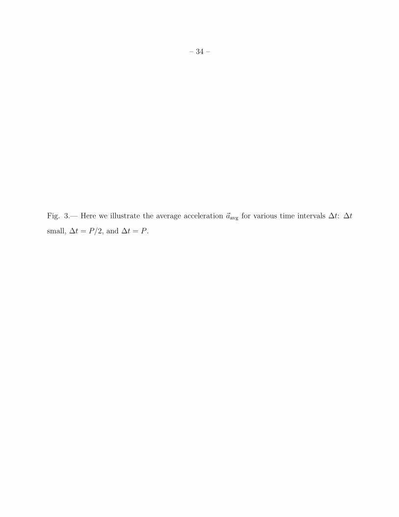
One can actually see that is that is likely from a simple picture. The average acceleration

over time ∆t is

~aavg =~v(t + ∆t) − ~v(t)

∆t. (69)

If the ∆t is long, then ~aavg is not in general center pointing. Say P is the period of the

uniform motion (i.e., the time to complete one cycle). If ∆t is P/2 or P , then ~aavg clearly is

not center pointing: in the first case, ~aavg = 2~v(t + ∆t)/∆t and in the second, ~aavg = 0. But

if ∆t becomes small, ~aavg plausibly looks more and more center pointing. Figure 3 illustrates

these cases.

– 34 –

Fig. 3.— Here we illustrate the average acceleration ~aavg for various time intervals ∆t: ∆t

small, ∆t = P/2, and ∆t = P .

– 35 –

In the limit as ∆t → 0, ~aavg becomes the instantaneous acceleration and it becomes cen-

ter pointing. One can show this rigorously and recover the centripetal acceleration formula

for ~a. We won’t do that since we’ve already got the centripetal acceleration formula.

The centripetal acceleration formula is often given in magnitude form or the form when

the inward radial direction is taken as positive: i.e.,

a =v2

r. (70)

This is, in fact, the formula most people remember—remember it.

Question for the class.

What is the period P (i.e., the time to complete one cycle) for uniform circular motion

given in terms of r and v?

You 30 seconds. Go.

Behold:

P =amount

rate=

circumference

|v|=

2πr

|v|, (71)

where you can drop the absolute value signs on v as long as you know you now mean the

magnitude of ~v.

9.1. Example: The Centripetal Acceleration of the Earth

What is the centripetal acceleration of the Earth about the Sun?

We assume the Earth’s orbit is circular and the motion uniform both of which are

approximately true.

Well we need v.

Let’s say we are given r = 1.496 × 1011 m which is the mean Sun-Earth distance and

– 36 –

fiducial period of 1 Julian year:

P = 1 Jyr = 365.25 days = 3.15576 × 107 s ≈ 1.0045096× π × 107 s ≈ π × 107 s . (72)

The exact period of revolution of the Earth around the Sun relative to the fixed stars is not

quite 1 Julian year, but 1 Julian year is good enough for here. The fact that a Julian year

is nearly π × 107 s is just a coincidence of our unit system, but its a useful way to remember

the year in seconds.

Now find v and a?

You have 2 minutes working in groups or individually. Go.

Behold:

v =2πr

P≈

2π × 1.5 × 1011

π × 107= 3.0 × 104 m/s = 30 km/s , (73)

where we’ve implicitly assumed that the direction the Earth is moving is the positive direction

which is conventional. Astrophysical velocities are frequently given in kilometers per second

because they are typically of order tens or hundreds or thousands of kilometers per second,

and so kilometers per second are a convenient unit for thinking of and remembering these

velocities.

The modern exact value for the mean orbital velocity is 29.783 km/s. But 30 km/s is

the value I always remember.

Also behold:

a =v2

r≈

9 × 108

1.5 × 1011= 6 × 10−3 m/s2 . (74)

A more exact calculation yields 5.93 × 10−3 m/s2. Not a memorable value.

Actually 5.93 × 10−3 m/s2 isn’t much of an acceleration compared to the acceleration

due to gravity near the Earth’s surface which has magnitude g.

What the fiducial value for g?

– 37 –

It’s g = 9.8 m/s2.

10. NON-UNIFORM CIRCULAR MOTION

11. RELATIVE MOTION

ACKNOWLEDGMENTS

Support for this work has been provided by the Department of Physics of the University

of Idaho and the Department of Physics of the University of Oklahoma.

REFERENCES

Arfken, G. 1970, Mathematical Methods for Physicists (New York: Academic Press)

Barger, V. D., & Olson, M. G. 1987, Classical Electricity and Magnetism (Boston: Allyn

and Bacon, Inc.)

Enge, H. A. 1966, Introduction to Nuclear Physics (Reading, Massachusetts: Addison-Wesley

Publishing Company)

French, A. P. 1971, Newtonian Mechanics: The M.I.T. Introductory Physics Series (New

York: W.W. Norton & Company)

Griffiths, D. J. 1999, Introduction to Electrodynamics (Upper Saddle River, New Jersey:

Prentice Hall)

Ohanian, H. C. 1988, Classical Electrodynamics (Boston: Allyn and Bacon, Inc.)

Serway, R. A. & Jewett, J. W., Jr. 2008, Physics for Scientists and Engineers, 7th Edition

(Belmont, California: Thomson)

– 38 –

Tipler, P. A., & Mosca, G. 2008, Physics for Scientists and Engineers, 6th Edition (New

York: W.H. Freeman and Company)

Weber, H. J., & Arfken, G. B. 2004, Essential Mathematical Methods for Physicists (Ams-

terdam: Elsevier Academic Press)

Wolfson, R. & Pasachoff, J. M. 1990, Physics: Extended with Modern Physics (London:

Scott, Foresman/Little, Brown Higher Education)

This preprint was prepared with the AAS LATEX macros v5.2.