Embed Size (px)
Citation preview

LARRY SNYDERDEPT. OF INDUSTRIAL AND SYSTEMS ENGINEERING
CENTER FOR VALUE CHAIN RESEARCH
LEHIGH UNIVERSITY
EWO SEMINAR SERIES – NOVEMBER 13, 2008
Multi-Echelon Inventory Optimization: An Overview
1

Outline
Introduction
Single-stage models (building blocks)
Multi-echelon modelsNetwork Topology
Deterministic Models
Stochastic Models
Decentralized systems
2

Introduction3

Factors Influencing Inventory Decisions
Why hold inventory?Lead timesEconomies of scale / fixed costs / quantity discountsService levelsConcerns about future availabilitySales / promotions
Why avoid inventory?Cost of capitalShelf spacePerishabilityRisk of theft / fire / etc.
4

Classifying Inventory Models
Deterministic vs. stochastic
Single- vs. multi-echelon
Periodic vs. continuous review
Discrete vs. continuous demand
Backorders vs. lost sales
Global vs. local control
Centralized vs. decentralized optimization
Fixed cost vs. no fixed cost
Lead time vs. no lead time
5

Costs in Inventory Models
Holding cost h ($ / item / unit time)
Stockout penalty p ($ / item / unit time)
Fixed cost k ($ / order)
Purchase cost c ($ / item)Often ignored in optimization models
6

A Brief History of Inventory Theory
Harris (1913): EOQ model
??? (19??): newsvendor model
Wagner and Whitin (1958): time-varying deterministic demands
Clark and Scarf (1960): serial stochastic systems
Roundy (1985): serial deterministic systems w/fixed costs, power-of-2 policies
Graves and Willems (2000): guaranteed-service models
7

(BUILDING BLOCKS)
Single-Stage Models8
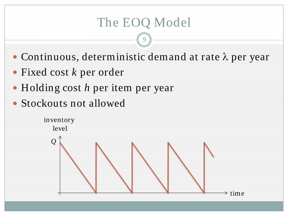
The EOQ Model
Continuous, deterministic demand at rate λ per year
Fixed cost k per order
Holding cost h per item per year
Stockouts not allowed
time
inventory level
Q
9

The EOQ Model: Optimization
Average annual cost:
First-order condition:
Optimal solution:
2)( hQ
QkQc +=λ
02
)(' 2 =+−=h
QkQc λ
hkQ λ2* = *2*)( hQhkQc == λ
10

The Newsvendor Model
Each day, newsvendor buys newspapers from publisher for $0.25 each
Sells newspapers for $0.75 each
Unsold papers are sold back to publisher for $0.10
Daily demand is stochastic, ~N(50, 102)
No inventory carryover [perishable inventory]
No backorder carryover [lost sales]
How many newspapers to buy?Probably >50, but how many?
11

A More General Formulation
Periodic, stochastic demandpdf f, cdf F
We’ll assume normal distribution (φ, Φ = standard normal)
Inventory carryover allowed [non-perishable] or notEither way, “overage” cost = h
May include salvage value/cost
Backorders or lost salesEither way, “underage” cost = p
May include lost profit, loss of goodwill, admin costs
Decision variable: base-stock level yIn each period, order up to y
12

Expected Cost Function
Convex ⇒ solve first-order condition (Leibniz’s rule)
Optimal solution:
where α = p / (p + h) (the newsvendor ratio)
∫∫∞
−+−=y
y
dxxfyxpdxxfxyhyc )()()()()(0
ασμσμ zhp
py +=⎟⎟⎠
⎞⎜⎜⎝
⎛+
Φ+= −1*
13

Interpretation of Optimal Solution14
No stockouts if demand ≤ μ + σzαOccurs with probability αα = optimal service level
If lead time (L) > 0:μ μ+σzα
ασμ zy +=*
cycle stock safety stock
LzLy ασμ +=*

PART 1:
NETWORK TOPOLOGY
15
Multi-Echelon Models

Network Topology16
System is composed of stages (nodes, items, sites…)Stages are grouped into echelonsStages can represent:
Physical locationsItems in BOMProcessing activities

Terminology17
Stages to the left are upstream
Those to the right are downstream
Downstream stages face customer demand
Network topologies, in increasing order of complexity:

Serial System
Each stage has at most one predecessor and at most one successor
18

Assembly System
Each stage has at most one successor
19

Distribution System
Each stage has at most one predecessor
20

Tree System
No restrictions on neighbors, but no cycles
21
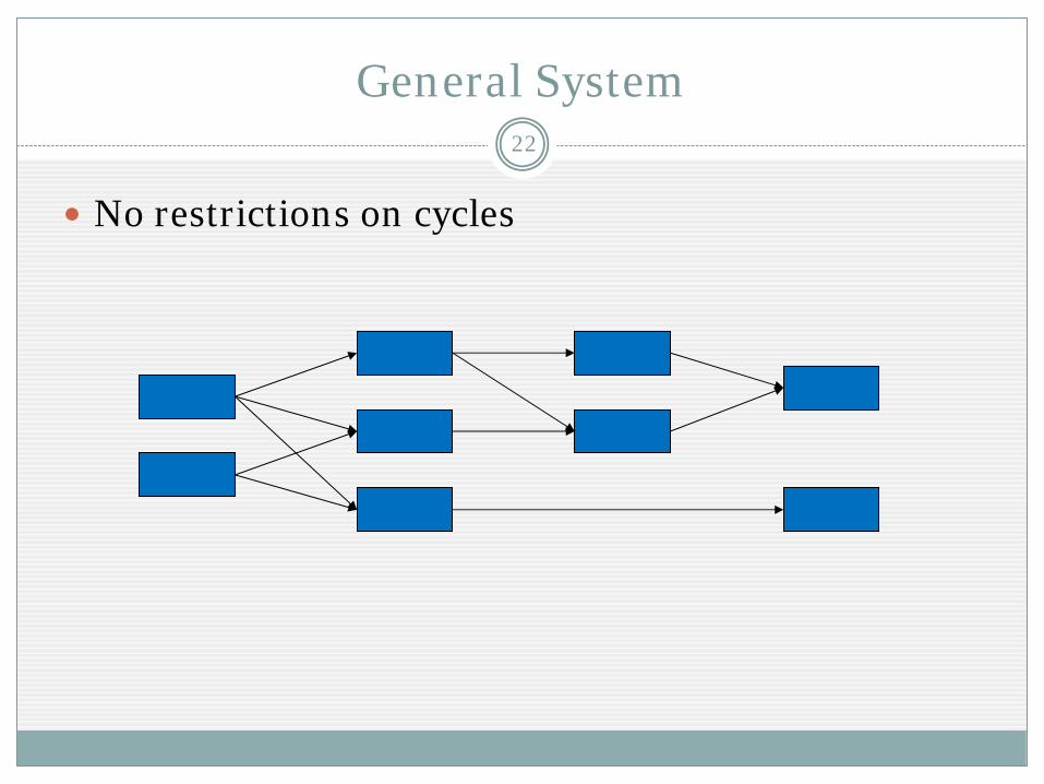
General System
No restrictions on cycles
22

PART 2:
DETERMINISTIC SYSTEMS
(WITH FIXED COSTS)
23
Multi-Echelon Models
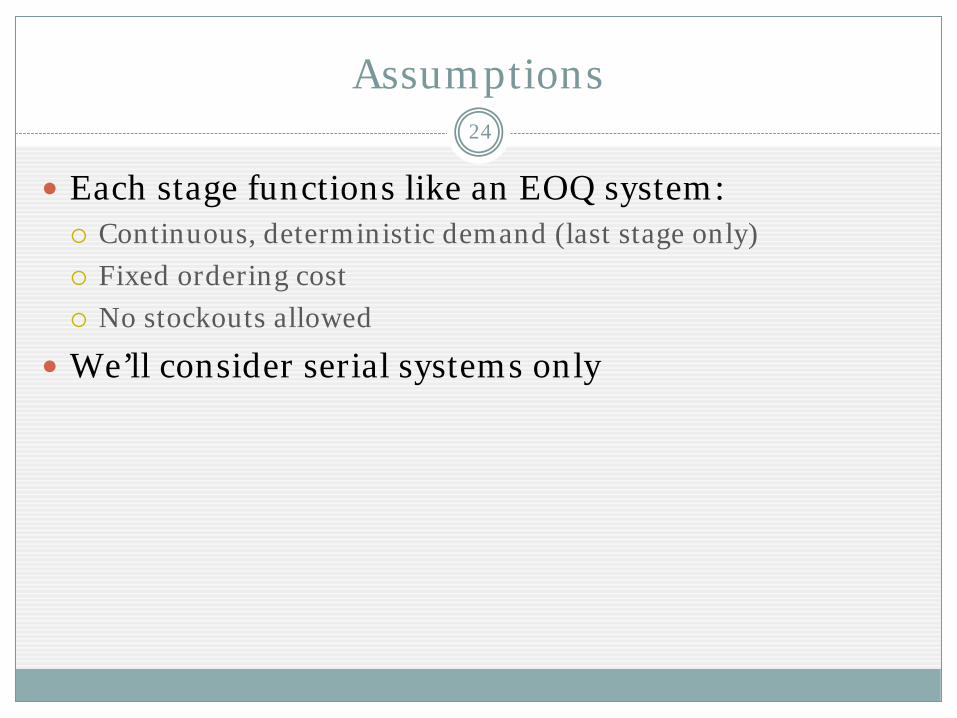
Assumptions24
Each stage functions like an EOQ system:Continuous, deterministic demand (last stage only)
Fixed ordering cost
No stockouts allowed
We’ll consider serial systems only

The Optimization Problem25
Need to choose Q at all stages simultaneously
Properties of optimal solutions:Zero-inventory ordering (ZIO): order only when inventory = 0Stationary: same Q for every order
(but different for different stages)
Nested: whenever one stage orders, so does its customer
Instead of optimizing over Q, we optimize over u (reorder interval)
u = Q / λ Q
u

NLIP Formulation26
Non-convex mixed-integer NLPOptimal solution u* is not known
In fact, no guarantee an optimal solution exists, except in limit
Therefore, get lower bound by solving relaxed problemAnd upper bound by rounding relaxed solution to feasible solution
},3,2,1{
0
s.t.
2)(min
1
…∈
≥
=
⎟⎟⎠
⎞⎜⎜⎝
⎛+=
+
∑
j
j
jjj
j
jj
j
j
u
uu
uhuk
C
θ
θ
λu

Relaxed Problem27
Convex NLP
Could solve using NLP solver
But there’s a better way…
0
s.t.)(min
1
≥
≥ +
j
jj
u
uuC u

Solving the Relaxed Problem28
Partition the stages:
In each partition, require every stage to have the same uj = u
Find u by solving EOQ—easy!
If we use the “correct” partition, we solve the relaxed problem
Find correct partition by finding upper concave envelope of set of points in 2D—easy!

Power-of-2 Policies29
Let û be a fixed base periode.g., 1 week, 3 days, etc.
Power-of-2 policy: each uj is an integer-power-of-2 multiple of û
To get feasible solution, round solution to relaxed problem to nearest power-of-2 policy
Power-of-2 policies are simple to implement and intuitive
(Stage 1 orders every 2 weeks, stage 2 orders every week, etc.)

Worst-Case Error Bound30
Let u* be the (unknown) optimal policy
Let u+ be the power-of-2 policy
Theorem (Roundy 1985): For any û,
If we can choose û, then the bound reduces to 1.02
06.122
3*)(
)(≈≤
+
uu
CC

PART 3:
STOCHASTIC SYSTEMS
(WITHOUT FIXED COSTS)
31
Multi-Echelon Models
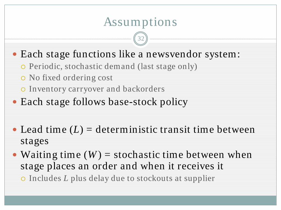
Assumptions32
Each stage functions like a newsvendor system:Periodic, stochastic demand (last stage only)No fixed ordering costInventory carryover and backorders
Each stage follows base-stock policy
Lead time (L) = deterministic transit time between stagesWaiting time (W) = stochastic time between when stage places an order and when it receives it
Includes L plus delay due to stockouts at supplier
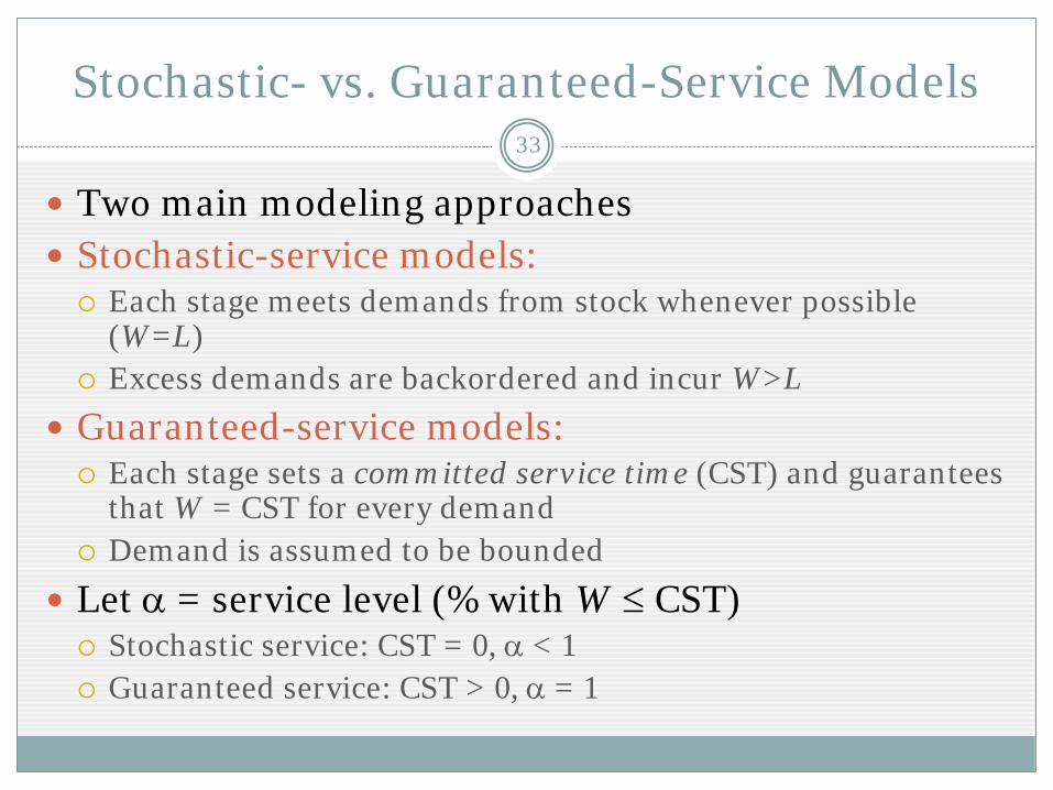
Stochastic- vs. Guaranteed-Service Models33
Two main modeling approachesStochastic-service models:
Each stage meets demands from stock whenever possible (W=L)Excess demands are backordered and incur W>L
Guaranteed-service models:Each stage sets a committed service time (CST) and guarantees that W = CST for every demandDemand is assumed to be bounded
Let α = service level (% with W ≤ CST)Stochastic service: CST = 0, α < 1Guaranteed service: CST > 0, α = 1

Stochastic-Service ModelsStochastic-Service Models
34

Serial Systems: The Clark-Scarf Algorithm35
Objective function:
E[on-hand] and E[backorders] at stage j depend on y at jand upstreamClark and Scarf (1960) rewrite c(y) so that system decomposes by stage
yj can be determined at each stage in sequenceUse decisions from downstream stages but ignore upstream onesAt each stage, solve 1-variable convex minimization problem(At last stage, it’s a newsvendor problem)
Easy computationally but cumbersome to implementGood heuristics exist: e.g., Shang and Song (1993)
[ ]∑ +=j
pEhEc ]backorders[]inventory hand-on[)(y

Assembly Systems36
Theorem (Rosling 1989): Every assembly system can be reduced to an equivalent serial system
Solve using Clark-Scarf algorithm
Based on inventory balance principle:
If inventory of 2 > inventory of 3, the extra is useless
Therefore, attempt to keep I2 = I3 at all times
2
31

Distribution Systems37
Inventory balance principle does not apply
Allocation rule becomes critical factor
The one-warehouse, multiple retailer (OWMR) systemFamous special case
Exact algorithm: Axsäter 1993
Heuristics: Sherbrooke 1968 (METRIC): approximate waiting time with its mean
Graves 1985: 2-moment approximation of backorder levels
Gallego, Özer, and Zipkin 2007: newsvendor approximation
Rong, Bulut, and Snyder 2008: decompose into serial systems

Extensions38
Fixed ordering costs
Stochastic lead times
Limited capacity
Imperfect quality
Some are hard, some are notTractability of standard problems is somewhat “fragile”

Guaranteed-Service ModelsGuaranteed-Service Models
39

Guaranteed-Service Models: Overview40
Each stage promises to deliver every item within a fixed number of periods
Called the committed service time (CST)
Requires assumption that demand is boundede.g., D ≤ μ + σzαEquivalently, ignore excess demand when D exceeds bound
CST assumption allows us to treat waiting time (W) as deterministic
References: Kimball 1955, Simpson 1958, Graves 1988, Graves and Willems 2000, 2003

Net Lead Time41
Each stage has:Processing time T
CST S
Net lead time (NLT) at stage i = Si+1 + Ti – Si
3 2 1T3 T2 T1
S3 S2 S1
“bad” LT “good” LT

Net Lead Time vs. Inventory42
Suppose Si = Si+1 + Tie.g., inbound CST = 4, proc time = 2, outbound CST = 6
Don’t need to hold any inventory
Operate entirely as pull (make-to-order, JIT) system
Suppose Si = 0Promise immediate order fulfillment
Make-to-stock system
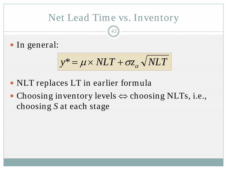
Net Lead Time vs. Inventory43
In general:
NLT replaces LT in earlier formula
Choosing inventory levels ⇔ choosing NLTs, i.e., choosing S at each stage
NLTzNLTy ασμ +×=*

Optimization44
Objective:Find optimal S values (CSTs)
To minimize expected holding cost
Subject to end-customer service requirement
Solution methods:Serial systems: dynamic programming (Graves 1988)
Tree systems: dynamic programming (Graves and Willems2000)
General systems: piecewise-linear approximation + CPLEX (Magnanti et al., 2006)

Key Insight45
It is usually optimal for only a few stages to hold inventory
Other stages operate as pull systems
Theorem (Graves 1988): In a serial system, every stage either:
holds zero inventory (and quotes maximum CST)
or quotes CST of zero (and holds maximum inventory)

Case Study
# below stage = processing time# in white box = CSTIn this solution, inventory is held of finished product and its raw materials
PART 1DALLAS ($260)
157
8
PART 2CHARLESTON ($7)
14
PART 4BALTIMORE ($220)
5
PART 3AUSTIN ($2)
14
6
8
5
PART 5CHICAGO ($155)
45
PART 7CHARLESTON ($30)
14
PART 6CHARLESTON ($2)
32
8
0
14
55
1445
14
32
(Adapted from Simchi-Levi, Chen, and Bramel, The Logic of Logistics, 2nd ed., Springer, 2004)
46

A Pure Pull System
Produce to order
Long CST to customer
No inventory held in system
PART 1DALLAS ($260)
157
8
PART 2CHARLESTON ($7)
14
PART 4BALTIMORE ($220)
5
PART 3AUSTIN ($2)
14
6
8
5
PART 5CHICAGO ($155)
45
PART 7CHARLESTON ($30)
14
PART 6CHARLESTON ($2)
32
8
77
14
55
1445
14
32
47

A Pure Push System
Produce to forecast
Zero CST to customer
Hold lots of finished goods inventory
PART 1DALLAS ($260)
157
8
PART 2CHARLESTON ($7)
14
PART 4BALTIMORE ($220)
5
PART 3AUSTIN ($2)
14
6
8
5
PART 5CHICAGO ($155)
45
PART 7CHARLESTON ($30)
14
PART 6CHARLESTON ($2)
32
8
0
14
55
1445
14
32
48

A Hybrid Push-Pull System
Part of system operated produce-to-stock, part produce-to-order
Moderate lead time to customer
PART 1DALLAS ($260)
157
8
PART 2CHARLESTON ($7)
14
PART 4BALTIMORE ($220)
5
PART 3AUSTIN ($2)
14
6
8
5
PART 5CHICAGO ($155)
45
PART 7CHARLESTON ($30)
14
PART 6CHARLESTON ($2)
32
8
30
7
8
945
14
32
push/pull boundary
49

CST vs. Inventory Cost
$0
$2,000
$4,000
$6,000
$8,000
$10,000
$12,000
$14,000
0 10 20 30 40 50 60 70 80
Committed Lead Time to Customer (days)
Inve
ntor
y Co
st ($
/yea
r)
Push System
Pull System
Push-Pull System
50

Optimization Shifts the Tradeoff Curve
$0
$2,000
$4,000
$6,000
$8,000
$10,000
$12,000
$14,000
0 10 20 30 40 50 60 70 80
Committed Lead Time to Customer (days)
Inve
ntor
y C
ost (
$/ye
ar)
51

52
Decentralized Systems

Decentralized Systems53
We have assumed the system is centralizedCan optimize at all stages globally
One stage may incur higher costs to benefit the system as a whole
What if each stage acts independently to minimize its own cost / maximize its own profit?
Suboptimality54
Optimizing locally results in suboptimalityExample: upstream stages want to operate make-to-order
Results in too much inventory downstream
Another example:Wholesaler chooses wholesale priceRetailer chooses order quantityOptimizing independently, the two parties will always leave money on the table

Supply Chain Contracts / Coordination55
One solution is for the parties to impose a contracting mechanism
Splits the costs / profits / risks / rewards
Still allows each party to act in its own best interest
If structured correctly, system achieves optimal cost / profit, even with parties acting selfishly
There is a large body of literature on contractingReview: Cachon 2003
Based on game theory
In practice, idea is commonly used
Actual OR models rarely implemented

Bullwhip Effect (BWE)56
Demand for diapers:
Time
Ord
er Q
uant
ity
consumption
consumer sales
retailer orders towholesaler
wholesaler orders tomanufacturer
manufacturer ordersto supplier

Irrational Behavior Causes BWE57
Firms over-react to demand signalsOrder too much when they perceive an upward demand trend
Then back off when they accumulate too much inventory
Firms under-weight the supply line
Both are irrational behaviors
Demonstrated by “beer game”
Sterman 1989

Rational Behavior Causes BWE58
BWE can be caused by rational behaviori.e., by acting in “optimal” ways according to OR inventory models
Four causes:Demand forecast updating
Batch ordering
Rationing game
Price variations
Lee, Padmanabhan, and Whang 1997

Further Reading59
Single-stage and multi-echelon stochastic-service models:Undergrad / MBA textbooks:
Simchi-Levi, Kaminsky, and Simchi-Levi, 3rd ed., 2007
Chopra and Meindl, 3rd ed., 2006
Nahmias, 5th ed., 2004
Graduate textbooks:Zipkin, 2000
Axsäter, 2nd ed., 2006
Porteus, 2002
Simchi-Levi, Chen, and Bramel, 2nd ed., 2004
Silver, Pyke, and Peterson, 3rd ed., 1998
Guaranteed-service models:Graves and Willems 2003 (book chapter)