Multi-Hazard Framework and Analysis of Soil-Bridge Systems

AN ABSTRACT OF THE THESIS OF

Trevor J Carey for the degree of Master of Science in Civil Engineering presented on

August 22, 2014.

Title: Multi-Hazard Framework and Analysis of Soil-Bridge Systems: Long

Duration Earthquake and Tsunami Loading

Abstract approved:

H. Benjamin Mason Andre R. Barbosa

During the 2011 Great East Japan Earthquake and Tsunami, numerous bridge struc

tures were damage or destroyed. The damage to bridge systems was caused by long

duration strong ground shaking, tsunami inundation forces, or both. Long dura

tion strong ground shaking from subduction zone earthquakes and the multi-hazard

scenario of combined earthquake and tsunami attack are particularly important in

the Pacific Northwest (PNW) where the Cascadia Subduction Zone is located. The

main ob jective of this thesis is to evaluate the safety and resilience of a typical PNW

coastal bridge to solely long duration strong ground shaking and to the combined

multi-hazard of a tsunami following an earthquake.

Bridge system design and research has predominantly focused on short duration

shallow crustal earthquakes, different from the long duration subduction zone earth

quake expected in the PNW. Although the peak design demands (i.e., deck drift

ratio) are typically the same for crustal and subduction zone motions, the duration

and number of loading cycles is not. By not considering the effects of earthquake

motion duration, the potential damage to a bridge system solely from a subduction

zone earthquake motion may be under-predicted. To examine the effects of earth

quake motion duration, a soil-bridge model was developed in the Open Systems for

Earthquake Engineering Simulation (OpenSees) framework and the soil-bridge system

response was evaluated for a suite of shallow crustal and subduction zone earthquake

motions. The crustal and subduction zone motions were linearly scaled to pronounce

ground motion duration and minimize amplitudinal differences. It was determined

that earthquake intensity parameters that do not account for earthquake motion du

ration are poor predictors of potential damage to soil-bridge systems when subjected

to subduction zone earthquake motions.

The combined multi-hazard scenario of long duration strong ground shaking and

tsunami attack extends two novel methods for determining hydrodynamic loading of

the soil-bridge model. The Particle Finite Element Method (PFEM) was used to

simulate impact of an idealized tsunami bore and the FEMA P-646 method was used

to simulate quasi-steady state long duration tsunami loading. Originally designed for

seismically induced lateral forces, the fluid-soil-bridge model was not able to resist

tsunami lateral loading. Furthermore, the preceding earthquake motion had little

effect on the fluid-soil-bridge models ability to resist hydrodynamic tsunami forces.

c©Copyright by Trevor J Carey August 22, 2014

All Rights Reserved

Multi-Hazard Framework and Analysis of Soil-Bridge Systems: Long Duration Earthquake and Tsunami Loading

by

Trevor J Carey

A THESIS

submitted to

Oregon State University

in partial fulfillment of the requirements for the

degree of

Master of Science

Presented August 22, 2014 Commencement June 2015

Master of Science thesis of Trevor J Carey presented on August 22, 2014.

APPROVED:

Co-Major Professor, representing Civil Engineering

Co-Major Professor, representing Civil Engineering

Head of the School of Civil and Construction Engineering

Dean of the Graduate School

I understand that my thesis will become part of the permanent collection of Oregon State University libraries. My signature below authorizes release of my thesis to any reader upon request.

Trevor J Carey, Author

ACKNOWLEDGEMENTS

This thesis would not have been possible without the help and support from numerous

individuals. First and foremost, I would like to thank my two advisors Dr. H.

Benjamin Mason, and Dr. Andre Barbosa for their unwavering support, guidance,

and mentoring. The successful completion of this thesis would not have been possible

without the endless time they committed. I would also like to thank Dr. Michael

H. Scott for his patience, and unofficial advising required for this thesis. With the

help and encouragement from these three educators I would not be continuing my

academic growth beyond this thesis.

Next, I would like to express my sincere thanks to Dr. Daniel Cox, and Dr.

Eugene Zhang for agreeing to serve on my graduate committee. To the other faculty

and staff of the School of Civil and Construction Engineering, thank you for your help

and support along my journey. To my friends I have met during my time at Oregon

State University, thank you for your friendship and advice.

I would like to acknowledge The Pacific Earthquake Engineering Research Center

(PEER), and Pacific Northwest Transportation Consortium (PacTrans) for providing

the necessary funding to conduct this research.

Finally, I would also like to extend my deepest appreciation to my father and

mother Pat and Virginia Carey for providing me an endless supply of encouragement

and love throughout my education. For this, I am eternally grateful.

TABLE OF CONTENTS

Page

1 Introduction . . . . . . . . . . . . . . . . . . . . . . . . . . . . . . . . . . . 1

2 Literature Review . . . . . . . . . . . . . . . . . . . . . . . . . . . . . . . . 4

2.1 Introduction . . . . . . . . . . . . . . . . . . . . . . . . . . . . . . . . . 4

2.2 Soil-Bridge Interaction . . . . . . . . . . . . . . . . . . . . . . . . . . . 4 2.2.1 Numerical Modeling of Soil-bridge Systems . . . . . . . . . . . 5

2.3 Tsunami Analysis of Bridge Systems . . . . . . . . . . . . . . . . . . . 10 2.3.1 Tsunami Modeling . . . . . . . . . . . . . . . . . . . . . . . . 12

3 Soil-Bridge Modeling Methodology . . . . . . . . . . . . . . . . . . . . . . 16

3.1 Introduction . . . . . . . . . . . . . . . . . . . . . . . . . . . . . . . . . 16

3.2 Earthquake Motion Selection . . . . . . . . . . . . . . . . . . . . . . . . 17

3.3 Soil Sites . . . . . . . . . . . . . . . . . . . . . . . . . . . . . . . . . . . 26

3.4 Soil-Pile Interface . . . . . . . . . . . . . . . . . . . . . . . . . . . . . . 31

3.5 Concrete Pile and Column . . . . . . . . . . . . . . . . . . . . . . . . . 36

3.6 Boundary Conditions . . . . . . . . . . . . . . . . . . . . . . . . . . . . 40

3.7 Bridge Deck and Abutments . . . . . . . . . . . . . . . . . . . . . . . . 41

3.8 Fundamental Periods and Damping . . . . . . . . . . . . . . . . . . . . 44

3.9 Analysis Framework . . . . . . . . . . . . . . . . . . . . . . . . . . . . 45

4 Long Duration Earthquake Motion Effects on Soil-Bridge Systems . . . . . 48

4.1 Inelastic Excursions . . . . . . . . . . . . . . . . . . . . . . . . . . . . . 48

5 Tsunami Analysis of the Fluid-Soil-Bridge System . . . . . . . . . . . . . . 86

5.1 Framework Steps . . . . . . . . . . . . . . . . . . . . . . . . . . . . . . 86

5.2 PFEM Procedure . . . . . . . . . . . . . . . . . . . . . . . . . . . . . . 87

5.3 PFEM Mesh . . . . . . . . . . . . . . . . . . . . . . . . . . . . . . . . . 88 5.3.1 Idealized Bore . . . . . . . . . . . . . . . . . . . . . . . . . . . 93

5.4 Steady State Hydrodynamic Forces . . . . . . . . . . . . . . . . . . . . 96

5.5 PFEM Impulsive Forces . . . . . . . . . . . . . . . . . . . . . . . . . . 97

5.6 Quasi-Steady-State Hydrodynamic Forces . . . . . . . . . . . . . . . . 101

6 Conclusion . . . . . . . . . . . . . . . . . . . . . . . . . . . . . . . . . . . . 109

6.1 Summary of Research . . . . . . . . . . . . . . . . . . . . . . . . . . . . 109

TABLE OF CONTENTS (Continued)

Page

6.2 Summary of Results . . . . . . . . . . . . . . . . . . . . . . . . . . . . 110

6.3 Future Work . . . . . . . . . . . . . . . . . . . . . . . . . . . . . . . . . 111

Bibliography . . . . . . . . . . . . . . . . . . . . . . . . . . . . . . . . . . . . 113

Appendices . . . . . . . . . . . . . . . . . . . . . . . . . . . . . . . . . . . . . 118

A Subduction Zone Ground Motions . . . . . . . . . . . . . . . . . . . . . 119

B Shallow Crustal Ground Motions . . . . . . . . . . . . . . . . . . . . . 123

LIST OF FIGURES

Figure Page

1.1 Directional components of the soil-bridge system (a) in-plane view of the longitudinal model (b) in-plane view of the transverse model. (pile foundation, and soil mesh not shown for clarity) . . . . . . . . . . . . 2

2.1 Idealization of base shear demands for a flexible-based system (i.e. includes SSI) with increased damping and period lengthening compared to a fixed-base system (NIST 2012). . . . . . . . . . . . . . . . . . . . 5

2.2 Two-dimensional soil profile of HBMC Bridge site (layer 1: Tertiary and Quaternary Alluvial deposits; layer 2: medium dense organic silt, sandy silt and stiff silty clay; layer 3: dense sand; layer 4: silt; layer 5: medium dense to dense silty sand and sand with some organic matter; layer 6: dense silty sand and sand; layer 7: soft or loose sandy silt or silty sand with organic matter; layer 8: soft to very soft organic silt with clay; and layer 9: abutment fill (Zhang et al. 2008). . . . . . . . 7

2.3 2-D soil mesh of the HBMC Bridge OpenSees model. Illustrated in Figure 2.2 is a detailed view of the modeled soil-profile (Zhang et al. 2008). . . . . . . . . . . . . . . . . . . . . . . . . . . . . . . . . . . . 8

2.4 2-D transverse bridge, soil column, and 1-D interface springs presented by Khosravifar (2012). . . . . . . . . . . . . . . . . . . . . . . . . . . 8

2.5 2-D longitudinal soil-bridge model presented by Barbosa et al. (2014). 9

2.6 Otsuchi Railroad Bridge with displaced deck, failed pier, and a detailed view of the failed connection (Chock et al. 2013). . . . . . . . . . . . 11

2.7 Failed pier of Otsuchi Railroad Bridge (Chock et al. 2013). . . . . . 11

2.8 Rikuzentakata bridge piers and abutments (left), and translated bridge deck (right) (Chock et al. 2013). . . . . . . . . . . . . . . . . . . . . . 12

2.9 Simulated water column collapse (Zhu and Scott 2014). . . . . . . . . 13

2.10 Comparison of OpenSees simulation and experimental results (Zhu and Scott 2014). . . . . . . . . . . . . . . . . . . . . . . . . . . . . . . . . 14

2.11 Tidal gage measurements for the 2004 Indian Ocean Tsunami. (a) Leading depression wave recorded at Ta Pho Noi, Thailand. (b) Leading elevation wave recorded at Titicorin, India. (Yeh 2009) . . . . . . 15

2.12 (a) Idealized tsunami bore front. (b) Hydraulic jump. (Mohamed 2008) 15

LIST OF FIGURES (Continued)

Figure Page

3.1 Conceptual bridge deck drawing showing longitudinal & transverse direction. (after. Shamsabadi et al. 2007) . . . . . . . . . . . . . . . . . 16

3.2 Directional components of the soil-bridge system (a) in-plane view of the longitudinal model (b) in-plane view of the transverse model. (pile foundation, and soil mesh not shown for clarity) . . . . . . . . . . . . 17

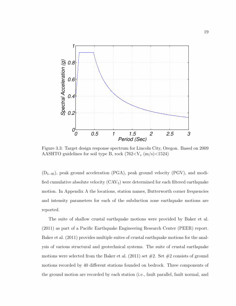
3.3 Target design response spectrum for Lincoln City, Oregon. Based on 2009 AASHTO guidelines for soil type B, rock (762<Vs (m/s)<1524) 19

3.4 Response spectrum for 46 Great East Japan Earthquake subduction zone motions plotted against AASHTO 2009 design response spectrum for Lincoln City, Oregon for soil type B. . . . . . . . . . . . . . . . . 23

3.5 Response spectrum for 48 shallow crustal motions plotted against the previously determined subduction zone median response spectrum, which was used at the target to scale the shallow crustal earthquake motions. 24

3.6 The relative difference between the median response of the shallow crustal and subduction zone spectra. . . . . . . . . . . . . . . . . . . 25

3.7 Liquefiable soil profile. . . . . . . . . . . . . . . . . . . . . . . . . . . 28

3.8 Generalized view of the far-field soil column modeled using 9-4 quadrilateral elements. Shown with lateral p-y soil interface springs. Not shown, vertical t-z, and end bearing q-z springs. . . . . . . . . . . . . 29

3.9 Deck displacement time series comparison for 20 m by 20 m and 20 m by 1 m mesh for the same shallow crustal motion (Irpinia, Italy-01). . 32

3.10 Comparison of the p-y springs resistance as a function of depth for the non-liquefiable and liquefiable soil profiles . . . . . . . . . . . . . . . 38

3.11 Reinforced concrete column and pile cross section. . . . . . . . . . . . 39

3.12 Cross section of the bridge deck used for the soil-bridge model (Barbosa et al. 2014). . . . . . . . . . . . . . . . . . . . . . . . . . . . . . . . . 42

3.13 Elastic perfectly plastic gap material force displacement response (Barbosa and Silva 2007). . . . . . . . . . . . . . . . . . . . . . . . . . . . 44

4.1 Visual illustration of plastic hinge rotation, θlp for shallow crustal motion 14, where Lp is the effective plastic hinge, φ is the curvature determined at time t and CPR is the cumulative plastic rotation. . . 51


Figure Page

4.2 Visual illustration of plastic hinge rotation, θlp for subduction zone motion 28, where Lp is the effective plastic hinge, φ is the curvature determined at time t and CPR is the cumulative plastic rotation. . . 52

4.3 Peak ground acceleration of subduction and shallow crustal earthquakes motions plotted against number of inelastic excursions for the longitudinal model with non-liquefiable site conditions. . . . . . . . . 53

4.4 Peak ground acceleration of subduction and shallow crustal earthquakes motions plotted against number of inelastic excursions for the longitudinal model with liquefiable site conditions. . . . . . . . . . . . 53

4.5 Peak ground acceleration of subduction and shallow crustal earthquakes motions plotted against number of inelastic excursions for the transverse model with non-liquefiable site conditions. . . . . . . . . . 54

4.6 Peak ground acceleration of subduction and shallow crustal earthquakes motions plotted against number of inelastic excursions for the transverse model with liquefiable site conditions. . . . . . . . . . . . . 54

4.7 Peak ground velocity of subduction and shallow crustal earthquakes motions plotted against number of inelastic excursions for the longitudinal model with non-liquefiable site conditions. . . . . . . . . . . . . 55

4.8 Peak ground velocity of subduction and shallow crustal earthquakes motions plotted against number of inelastic excursions for the longitudinal model with liquefiable site conditions. . . . . . . . . . . . . . . 55

4.9 Peak ground velocity of subduction and shallow crustal earthquakes motions plotted against number of inelastic excursions for the transverse model with non-liquefiable site conditions. . . . . . . . . . . . . 56

4.10 Peak ground velocity of subduction and shallow crustal earthquakes motions plotted against number of inelastic excursions for the transverse model with liquefiable site conditions. . . . . . . . . . . . . . . 56

4.11 Arias intensity of subduction and shallow crustal earthquakes motions plotted against number of inelastic excursions for the longitudinal model with non-liquefiable site conditions. . . . . . . . . . . . . . . . 57

4.12 Arias intensity of subduction and shallow crustal earthquakes motions plotted against number of inelastic excursions for the longitudinal model with liquefiable site conditions. . . . . . . . . . . . . . . . . . . 57


Figure Page

4.13 Arias intensity of subduction and shallow crustal earthquakes motions plotted against number of inelastic excursions for the transverse model with non-liquefiable site conditions. . . . . . . . . . . . . . . . . . . . 58

4.14 Arias intensity of subduction and shallow crustal earthquakes motions plotted against number of inelastic excursions for the transverse model with liquefiable site conditions. . . . . . . . . . . . . . . . . . . . . . 58

4.15 Spectral Acceleration at T1 of subduction and shallow crustal earthquakes motions plotted against number of inelastic excursions for the longitudinal model with non-liquefiable site conditions. . . . . . . . . 59

4.16 Spectral Acceleration at T1 of subduction and shallow crustal earthquakes motions plotted against number of inelastic excursions for the longitudinal model with liquefiable site conditions. . . . . . . . . . . . 59

4.17 Spectral Acceleration at T1 of subduction and shallow crustal earthquakes motions plotted against number of inelastic excursions for the transverse model with non-liquefiable site conditions. . . . . . . . . . 60

4.18 Spectral Acceleration at T1 of subduction and shallow crustal earthquakes motions plotted against number of inelastic excursions for the transverse model with liquefiable site conditions. . . . . . . . . . . . . 60

4.19 Significant duration of subduction and shallow crustal earthquakes motions plotted against number of inelastic excursions for the longitudinal model with non-liquefiable site conditions. . . . . . . . . . . . . . . . 61

4.20 Significant duration of subduction and shallow crustal earthquakes motions plotted against number of inelastic excursions for the longitudinal model with liquefiable site conditions. . . . . . . . . . . . . . . . . . . 61

4.21 Significant duration of subduction and shallow crustal earthquakes motions plotted against number of inelastic excursions for the transverse model with non-liquefiable site conditions. . . . . . . . . . . . . . . . 62

4.22 Significant duration of subduction and shallow crustal earthquakes motions plotted against number of inelastic excursions for the transverse model with liquefiable site conditions. . . . . . . . . . . . . . . . . . . 62

4.23 Cumulative absolute velocity five of subduction and shallow crustal earthquakes motions plotted against number of inelastic excursions for the longitudinal model with non-liquefiable site conditions. . . . . . . 63


Figure Page

4.24 Cumulative absolute velocity five of subduction and shallow crustal earthquakes motions plotted against number of inelastic excursions for the longitudinal model with liquefiable site conditions. . . . . . . . . 63

4.25 Cumulative absolute velocity five of subduction and shallow crustal earthquakes motions plotted against number of inelastic excursions for the transverse model with non-liquefiable site conditions. . . . . . . . 64

4.26 Cumulative absolute velocity five of subduction and shallow crustal earthquakes motions plotted against number of inelastic excursions for the transverse model with liquefiable site conditions. . . . . . . . . . 64

4.27 Peak ground acceleration of subduction and shallow crustal earthquakes motions plotted against cumulative plastic rotation for the longitudinal model with non-liquefiable site conditions. . . . . . . . . . . 65

4.28 Peak ground acceleration of subduction and shallow crustal earthquakes motions plotted against cumulative plastic rotation for the longitudinal model with liquefiable site conditions. . . . . . . . . . . . . 65

4.29 Peak ground acceleration of subduction and shallow crustal earthquakes motions plotted against cumulative plastic rotation for the transverse model with non-liquefiable site conditions. . . . . . . . . . 66

4.30 Peak ground acceleration of subduction and shallow crustal earthquakes motions plotted against cumulative plastic rotation for the transverse model with liquefiable site conditions. . . . . . . . . . . . . 66

4.31 Peak ground velocity of subduction and shallow crustal earthquakes motions plotted against cumulative plastic rotation for the longitudinal model with non-liquefiable site conditions. . . . . . . . . . . . . . . . 67

4.32 Peak ground velocity of subduction and shallow crustal earthquakes motions plotted against cumulative plastic rotation for the longitudinal model with liquefiable site conditions. . . . . . . . . . . . . . . . . . . 67

4.33 Peak ground velocity of subduction and shallow crustal earthquakes motions plotted against cumulative plastic rotation for the transverse model with non-liquefiable site conditions. . . . . . . . . . . . . . . . 68

4.34 Peak ground velocity of subduction and shallow crustal earthquakes motions plotted against cumulative plastic rotation for the transverse model with liquefiable site conditions. . . . . . . . . . . . . . . . . . . 68


Figure Page

4.35 Arias intensity of subduction and shallow crustal earthquakes motions plotted against cumulative plastic rotation for the longitudinal model with non-liquefiable site conditions. . . . . . . . . . . . . . . . . . . . 69

4.36 Arias intensity of subduction and shallow crustal earthquakes motions plotted against cumulative plastic rotation for the longitudinal model with liquefiable site conditions. . . . . . . . . . . . . . . . . . . . . . 69

4.37 Arias intensity of subduction and shallow crustal earthquakes motions plotted against cumulative plastic rotation for the transverse model with non-liquefiable site conditions. . . . . . . . . . . . . . . . . . . . 70

4.38 Arias intensity of subduction and shallow crustal earthquakes motions plotted against cumulative plastic rotation for the transverse model with liquefiable site conditions. . . . . . . . . . . . . . . . . . . . . . 70

4.39 Spectral Acceleration at T1 of subduction and shallow crustal earthquakes motions plotted against cumulative plastic rotation for the longitudinal model with non-liquefiable site conditions. . . . . . . . . . . 71

4.40 Spectral Acceleration at T1 of subduction and shallow crustal earthquakes motions plotted against cumulative plastic rotation for the longitudinal model with liquefiable site conditions. . . . . . . . . . . . . 71

4.41 Spectral Acceleration at T1 of subduction and shallow crustal earthquakes motions plotted against cumulative plastic rotation for the transverse model with non-liquefiable site conditions. . . . . . . . . . 72

4.42 Spectral Acceleration at T1 of subduction and shallow crustal earthquakes motions plotted against cumulative plastic rotation for the transverse model with liquefiable site conditions. . . . . . . . . . . . . 72

4.43 Significant duration of subduction and shallow crustal earthquakes motions plotted against cumulative plastic rotation for the longitudinal model with non-liquefiable site conditions. . . . . . . . . . . . . . . . 73

4.44 Significant duration of subduction and shallow crustal earthquakes motions plotted against cumulative plastic rotation for the longitudinal model with liquefiable site conditions. . . . . . . . . . . . . . . . . . . 73

4.45 Significant duration of subduction and shallow crustal earthquakes motions plotted against cumulative plastic rotation for the transverse model with non-liquefiable site conditions. . . . . . . . . . . . . . . . 74


Figure Page

4.46 Significant duration of subduction and shallow crustal earthquakes motions plotted against cumulative plastic rotation for the transverse model with liquefiable site conditions. . . . . . . . . . . . . . . . . . . 74

4.47 Cumulative absolute velocity five of subduction and shallow crustal earthquakes motions plotted against cumulative plastic rotation for the longitudinal model with non-liquefiable site conditions. . . . . . . 75

4.48 Cumulative absolute velocity five of subduction and shallow crustal earthquakes motions plotted against cumulative plastic rotation for the longitudinal model with liquefiable site conditions. . . . . . . . . 75

4.49 Cumulative absolute velocity five of subduction and shallow crustal earthquakes motions plotted against cumulative plastic rotation for the transverse model with non-liquefiable site conditions. . . . . . . . 76

4.50 Cumulative absolute velocity five of subduction and shallow crustal earthquakes motions plotted against cumulative plastic rotation for the transverse model with liquefiable site conditions. . . . . . . . . . 76

5.1 Conceptual drawing of the numerical wave flume and idealized bore with critical dimensions labeled (i.e. h1, h0, and η). Soil and pile-foundation not shown for clarity (Carey et al. 2014). . . . . . . . . . . 89

5.2 2 m x 2 m static fluid tank used to illustrate mesh refinement . . . . 90

5.3 Effect of mesh refinement on normalized error (3.4) and normalized computational time (8539 seconds). . . . . . . . . . . . . . . . . . . . 92

5.4 Detailed schematic of the three velocity regions of the PFEM model (i.e idealized bore, standing fluid and transition region). . . . . . . . . 95

5.5 Resolved horizontal force time history at the bridge deck-column connection for idealized bore 22. . . . . . . . . . . . . . . . . . . . . . . . 99

5.6 Resolved vertical force time history at the bridge deck-column connection for idealized bore 22 . . . . . . . . . . . . . . . . . . . . . . . . . 99

5.7 Resolved rotational moment time history at the bridge deck-column connection for idealized bore 22. . . . . . . . . . . . . . . . . . . . . . 100

5.8 Conceptualization of earthquake-tsunami interaction diagram, with dots representing unique analysis runs. . . . . . . . . . . . . . . . . . 101

5.9 Earthquake-tsunami interaction diagram for subduction fault parallel motion FKSH12. . . . . . . . . . . . . . . . . . . . . . . . . . . . . . 105


Figure Page

5.10 Earthquake-tsunami interaction diagram momentum flux hu2 plotted against deck drift ratio (%). . . . . . . . . . . . . . . . . . . . . . . . 106

LIST OF TABLES

Table Page

3.1 Soil pressure dependent multi-yield (PDMY) parameters for fully saturated dense (DR = 90%) and loose (DR = 35%) sands (Yang et al. 2003). . . . . . . . . . . . . . . . . . . . . . . . . . . . . . . . . . . . 27

3.2 Summary of 1-D lateral p-y soil-interface spring values for the non-liquefiable site-soil conditions . . . . . . . . . . . . . . . . . . . . . . 34

3.3 Summary of 1-D vertical t-z soil-interface spring values for the non-liquefiable site-soil conditions . . . . . . . . . . . . . . . . . . . . . . 35

3.4 Unreduced and reduced strength and stiffness parameters for p-y springs in accordance with McGann et al. (2011).The liquefiable layer is highlighted. . . . . . . . . . . . . . . . . . . . . . . . . . . . . . . . . . . . 37

4.1 Correlation coefficients for the longitudinal model with subduction zone ground motions . . . . . . . . . . . . . . . . . . . . . . . . . . . 77

4.2 Correlation coefficients for the longitudinal model with shallow crustal ground motions . . . . . . . . . . . . . . . . . . . . . . . . . . . . . . 78

4.3 Correlation coefficients for the transverse model with subduction zone ground motions . . . . . . . . . . . . . . . . . . . . . . . . . . . . . . 79

4.4 Correlation coefficients for the transverse model with shallow crustal ground motions . . . . . . . . . . . . . . . . . . . . . . . . . . . . . . 80

4.5 Number of inelastic excursions observed for crustal motions . . . . . . 81

4.6 Number of inelastic excursions observed for subduction zone motions 82

4.7 Summary table of NIE and CPR for shallow crustal earthquakes . . . 83

4.8 Summary table of NIE and CPR for subduction zone earthquakes . . 83

5.1 Number of elements and DOFs with corresponding mesh refinement. . 91

5.2 Tsunami bore characteristics h1, h0, u0, & η seen in Figure 5.1 for each of the 24 tsunami bores considered. . . . . . . . . . . . . . . . . . . . 94

5.3 Peak horizontal force, vertical force, and moment for each of the 24 idealized tsunami bores resolved at the bridge deck-column connection. 98

5.4 Quasi-steady-state hydrodynamic forces applied to the transverse fluidsoil-bridge model. . . . . . . . . . . . . . . . . . . . . . . . . . . . . . 104

5.5 107

LIST OF TABLES (Continued)

Table Page

Tsunami and earthquake intensity measures for the 12 ground motions considered. . . . . . . . . . . . . . . . . . . . . . . . . . . . . . . . . .

LIST OF APPENDIX TABLES

Table Page

A.1 Subduction zone ground motion station, location & component . . . . 120

A.2 Intensity parameters for baseline corrected and filterd motions. . . . . 121

A.3 Linear scaled ground motion intensity parameters . . . . . . . . . . . 122

B.1 Shallow crustal motion station, location, and component . . . . . . . 124

B.2 Intensity parameters for crustal motions prior to linear scaling . . . . 125

B.3 Crustal linear sclaed ground motion intensity parameters . . . . . . . 126

Chapter 1: Introduction

The recent Great East Japan Earthquake and Tsunami emphasized the multi-hazard

scenario of a large earthquake followed by a devastating tsunami. Damage to bridge-

structures during the earthquake and tsunami is particularly important, because re

gional recovery heavily depends on the operation of bridges to move supplies and

equipment. Like Japan, the Pacific Northwest (PNW) also experiences devastating

mega-thrust earthquakes and large local tsunamis. Understanding these hazards is

critical, because PNW coastal bridges may not be adequately designed for long du

ration strong ground shaking or the combined scenario of a tsunami following an

earthquake. The ob jective of this work is to determine the safety and resilience of

a typical PNW coastal bridge to the expected long duration earthquake, and the

combined multi-hazard case of a tsunami following an earthquake.

A soil-bridge system was numerically modeled to determine the seismic and hy

drodynamic response of a typical PNW coastal bridge. The longitudinal and trans

verse components of the soil-bridge system (earthquake hazard only) and the fluid

soil-bridge system (combined tsunami and earthquake hazard) are illustrated in Fig

ure 1.1. The numerical soil-bridge system was developed using the OpenSees finite

element framework (McKenna et al. 2010).

Soil-bridge systems have been predominately designed for amplitudinal intensity

parameters with no consideration of earthquake motion duration. To determine how

the duration of an earthquake can cause damage to soil-bridge systems, a suite of 46

subduction zone, and 48 shallow crustal motions were selected. All ground motions

were linearly scaled to the same target spectrum to isolate ground motion duration ef

2

Figure 1.1: Directional components of the soil-bridge system (a) in-plane view of the longitudinal model (b) in-plane view of the transverse model. (pile foundation, and soil mesh not shown for clarity)

fects. The analyses was performed with four different soil-bridge model configurations.

In addition to the transverse and longitudinal bridge orientations, a non-liquefiable

and liquefiable site-soil condition was also included. The four soil-bridge model con

figurations extend the singular configuration by Barbosa et al. (2014) for a similar

soil-bridge model.

The tsunami loading for the multi-hazard scenario was applied to the fluid-soil

bridge model with two different methods. The Particle Finite Element Method

(PFEM) was used to numerically generate 24 idealized tsunami bores to simulate

various cases of tsunami attack. The FEMA P-646 (2008) hydrodynamic force equa

tion was used to simulate quasi-steady state tsunami loading with changes in flow

depth and velocity occurring over long periods of time. To express the combined

damage to the fluid-soil-bridge system, an earthquake-tsunami interaction diagram is

proposed herein to illustrate the damage from both hazards.

The OpenSees finite element framework has been used by researchers for the last

decade to perform advanced structural and geotechnical earthquake simulations (e.g.,

Fragiadakis et al. 2006; Zhang et al. 2008). The diverse assortment of constitutive

models, solution algorithms and element formulations in the OpenSees framework al

lows for the aggregation of damage for successive earthquake and tsunami simulations.

3

Allowing for the aggregation of damage is important, because the degradation of the

fluid-soil-bridge model following the earthquake simulation would not be captured

with an uncoupled analysis.

The work consists of four main sections. The first section reviews the current liter

ature on soil-bridge modeling, numerical tsunami loading methods, and tsunami wave

types. The second section presents the methodology used to numerically model the

soil-bridge system. This section also includes methodology on the non-liquefiable and

liquefiable site-soil conditions, and the development of the longitudinal and transverse

bridge orientations. The third section presents comparisons between short duration

shallow crustal earthquakes, and long duration subduction zone earthquakes. The

forth section presents the methodology to extend the two methods to simulate tsunami

loading to the fluid-soil-bridge model. This section concludes with the results of the

multi-hazard scenario for both the PFEM and FEMA P-646 (2008) hydrodynamic

methods.

4

Chapter 2: Literature Review

2.1 Introduction

The review of the current literature is separated into two sections. The first sec

tion focuses on numerical modeling of soil-bridge systems. Previous researchers have

developed modeling frameworks for multiple bridge orientations, liquefiable and non-

liquefiable site-soil conditions, and simulated pre-and-post construction soil condi

tions. The second section of the literature review presents novel methods to nu

merically simulate tsunami wave loading using the Particle Finite Element Method

(PFEM). Also summarized is a brief description of an idealized tsunami bore, and

common tsunami types.

2.2 Soil-Bridge Interaction

Soil-structure interaction (SSI) has been considered by engineering researchers and

practitioners to accurately evaluate the seismic response of soil-bridge systems. Bridge-

systems that incorporate SSI have longer fundamental periods and increased system

damping compared with fixed-base bridge-systems. Typically, SSI has been thought

to only benefit bridge-systems, because seismic demands are reduced. Depending on

the earthquake motion and the flexible-base foundation period shift, seismic demands

may actually increase. Figure 2.1 illustrates that SSI does not always reduce seis

mic demands depending on the ground motion and period shift. The uncertainty of

seismic demands is the primary motivation for including SSI in the bridge system

5

analysis. Soil-bridge system literature presented in this chapter is neither exhaustive

nor focused explicitly on basic SSI principals. For a comprehensive discussion on SSI

Kausel (2010) provides early history of SSI research and advances.

Figure 2.1: Idealization of base shear demands for a flexible-based system (i.e. includes SSI) with increased damping and period lengthening compared to a fixed-base system (NIST 2012).

2.2.1 Numerical Modeling of Soil-bridge Systems

One of the first numerical soil-bridge models created with the (OpenSees) framework

(McKenna et al. 2010) was developed by Zhang et al. (2008) for the Humboldt Bay

Middle Channel (HBMC) Bridge. The bridge deck of the HBMC Bridge is cast-in

place reinforced concrete and is supported by four precast, prestressed I-girders. The

bridge deck and girders are assumed to respond linearly elastically during loading,

given the high axial stiffness of the girder-bridge-deck composite. The bridge girders

are supported by nine reinforced concrete piers that transmit forces and rotational

6

moments to the soil continuum. The nine reinforced concrete piers are modeled in

OpenSees using the Mander et al. (1988) confined concrete model and are discretized

using fiber sections and beam-column elements. The modeled soil continuum, which

is illustrated in Figure 2.2, incorporates liquefiable layers beneath and atop a com

petent non-liquefiable layer. The soil continuum is represented with a far-field mesh

composed of 4 node “u-p” quadrilateral, plane-strain elements (Elgamal et al. 2002)

that combine soil-skeleton displacement (u) and pore water pressure (p). The far-field

mesh and structural bridge model are shown in Figure 2.3. Zhang et al. (2008) con

cluded the seismic response of the soil-bridge system was controlled by the nonlinear

inelastic response of the soil continuum. Plastic deformation of the soil caused by

lateral spreading and liquefaction resulted in large residual deformations and internal

forces.

Khosravifar (2012) developed a 2D nonlinear inelastic soil-bridge model for a sin

gle pile-foundation shaft. The model illustrated in Figure 2.4 was used to evaluate

the inelastic structural response from effects of liquefaction and lateral spreading.

Additionally, Khosravifar (2012) performed a parametric study to determine which

system parameters had the greatest effect on the response of the soil-bridge system to

earthquake loading. The soil-bridge model developed by Khosravifar (2012) consid

ered the transverse direction of a typical pre-stressed box-beam bridge. The tributary

mass and gravity loads were lumped at the bridge deck.

The soil profile Khosravifar (2012) selected consisted of a 5 m clay crust, 3 m

loose liquefiable sand and 12 m dense non-liquefiable sand. The soil-profile was dis

cretized to a far-field soil column consisting of 9 node “u-p” quadrilateral elements.

The pressure independent multi-yield material was used to model clays, and the pres

sure dependent multi-yield material was used to model sands. The soil column was

attached to the pile-foundation with one dimensional lateral p-y, vertical t-z, and

7

Figure 2.2: Two-dimensional soil profile of HBMC Bridge site (layer 1: Tertiary and Quaternary Alluvial deposits; layer 2: medium dense organic silt, sandy silt and stiff silty clay; layer 3: dense sand; layer 4: silt; layer 5: medium dense to dense silty sand and sand with some organic matter; layer 6: dense silty sand and sand; layer 7: soft or loose sandy silt or silty sand with organic matter; layer 8: soft to very soft organic silt with clay; and layer 9: abutment fill (Zhang et al. 2008).

end bearing q-z soil interface springs. The spring coefficients were developed using

recommendations from the American Petroleum Institute (API 1993), with modifica

tions to the lateral p-y springs using a procedure proposed by Boulanger et al. (1999)

to account for larger effective overburden stresses. Similar to the soil-bridge model

presented by Zhang et al. (2008), the column and pile-foundation was a continuous

reinforced concrete shaft that was discretized into a fiber section for use with beam

column elements.

8

Figure 2.3: 2-D soil mesh of the HBMC Bridge OpenSees model. Illustrated in Figure 2.2 is a detailed view of the modeled soil-profile (Zhang et al. 2008).

Figure 2.4: 2-D transverse bridge, soil column, and 1-D interface springs presented by Khosravifar (2012).

9

Khosravifar (2012) showed the combined effect of structural inertial forces and

lateral spreading produced greater demands than the isolated case of non-liquefaction

or lateral spreading. Khosravifar (2012) concluded that to determine the correct

seismic response of a bridge-system, the analysis needs to consider all components

(i.e. bridge deck, column, pile, soil) and non-linear material response.

Barbosa et al. (2014) used work by Zhang et al. (2008) and Khosravifar (2012)

as motivation to develop the 2-D nonlinear longitudinal soil-bridge model illustrated

in Figure 2.5. The soil-bridge model presented by Barbosa et al. (2014) was a 63.4

m long reinforced concrete bridge supported by a center column and end abutments,

which was adapted from a model presented by Shamsabadi et al. (2007).

Figure 2.5: 2-D longitudinal soil-bridge model presented by Barbosa et al. (2014).

The soil-bridge modeling effort herein closely follows the assumptions, and method

ologies developed by Barbosa et al. (2014). A comprehensive description of the soil-

bridge model by Barbosa et al. (2014) with minor alterations is forthcoming in Chap

ter 3.

10

2.3 Tsunami Analysis of Bridge Systems

The devastating March 11, 2011 Great East Japan Earthquake and Tsunami resulted

in 20,000 fatalities and caused over $217 billion in damage (Chock et al. 2013). Ac

cordingly, the 2011 event is the most costly natural disaster in history, in terms of

monetary losses. Tsunami damage was observed in buildings, seawalls, tsunami barri

ers, piers, storage tanks, bridges, and to other engineered systems. Damage to bridge

systems from tsunami inundation was caused by multiple mechanisms; for example,

location and orientation, bridge type (i.e. simply supported, or fixed connections),

soil instability and uplift restraints. A select number of bridge failures from tsunami

attack are detailed in this chapter.

The multi-span Otsuchi Railroad Bridge, shown in Figures 2.6 and 2.7, experi

enced a total system failure during the tsunami (Chock et al. 2013). The deep girders

required to support rail car loading produced a large exposed area, which resulted in

extreme lateral loads during inundation. The induced hydrodynamic loading caused

either the connection to fail at the girder-pier interface, or the pier to fail by flexure

at the ground surface. Connection failure is illustrated in Figure 2.6, and pier failure

is illustrated in Figure 2.7. Chock et al. (2013) calculated that the fully inundated

pier could resist a maximum flow velocity of 3.9 m/s with the bridge deck attached

and 11.2 m/s without the bridge-deck.

The three-span Rikuzentakata automobile bridge is shown in Figure 2.8 (Chock

et al. 2013). An evaluation of the Rikuzentakata Bridge revealed that the piers

and abutments showed no signs of damage from the tsunami attack. Although the

substructure remained undamaged, the simply-supported bridge deck was relocated

40 m upland from the substructure. Chock et al. (2013) showed that the bridge deck

translation likely resulted from buoyant forces when the deck was fully submerged

11

Figure 2.6: Otsuchi Railroad Bridge with displaced deck, failed pier, and a detailed view of the failed connection (Chock et al. 2013).

Figure 2.7: Failed pier of Otsuchi Railroad Bridge (Chock et al. 2013).

rather than lateral forces on the girder face. The argument put forth by Chock et al.

(2013) was further validated with inspection of bridge abutments where steel dowel

bars used to prevent lateral movement of the deck remained intact. The undamaged

dowel bars suggest that the bridge deck was lifted with buoyant forces rather then

pushed by lateral forces.

The uplift of the Rikuzentakata automobile bridge was not influenced by the pre

ceding earthquake, but the pier failure experienced at the Otsuchi Railroad Bridge

12

Figure 2.8: Rikuzentakata bridge piers and abutments (left), and translated bridge deck (right) (Chock et al. 2013).

may have been affected by the earthquake. Initial earthquake damage can be difficult

to distinguish, because an assessment of the bridge system cannot be performed fol

lowing the earthquake but preceding tsunami attack. The purpose of this section is to

present newly developed methods for simulating tsunami loading on bridge structures.

2.3.1 Tsunami Modeling

The Particle Finite Element Method (PFEM), which uses a Lagrangian formulation

for both fluid and solid domains, has been used by researchers to simulate fluid-

structure interaction problems (i.e., Onate et al. 2004; Idelsohn et al. 2006). The

Lagrangian formulation is favorable, because the motion of each individual fluid par

ticle is tracked, which is preferred for free fluid surface wave problems (Zhu and Scott

2014). Another important benefit of the PFEM procedure is that the Lagrangian

formulation of the fluid domain is easily adaptable to the Lagrangian formulation

used for structural mechanics (Zhu and Scott 2014). The disadvantage of tracking

individual particles with the Lagrangian formulation is mesh updating is required at

13

the end of each analysis time step which increases computational cost.

The PFEM was extended to the OpenSees framework by Zhu and Scott (2014).

Zhu and Scott (2014) performed numerous validation and variation tests of the im

plemented PFEM in OpenSees. The validation tests analyzed fluid sloshing in a tank

and a static water column collapse. As an example, Zhu and Scott (2014) compared

the water column collapse illustrated in Figure 2.9 at discrete time steps to experi

mental data for a similar problem. The simulated water column was discretized with

1392 nodes and 2429 elements, and the time step selected for the analysis was 0.001

seconds (Zhu and Scott 2014). Comparison of the simulated and experiential results

are shown in Figure 2.10 for the location of the leading edge of the water column,

and change in water column height.

Figure 2.9: Simulated water column collapse (Zhu and Scott 2014).

The leading edge of the water column collapse in Figure 2.10a shows that the

14

Figure 2.10: Comparison of OpenSees simulation and experimental results (Zhu and Scott 2014).

OpenSees analysis predicted a slightly higher velocity than the experimental results.

However, observed velocity difference can be attributed to the frictional forces between

the fluid and experimental wave flume, which have been not included in the OpenSees

PFEM simulation. The simulated accuracy predicted the change in the experimental

fluid column height which is reported in Figure 2.10b.

Two common tsunami waveforms are leading elevation and leading depression

waves (Yeh 2009). Leading elevation waves experience a wave crest, which is followed

by a wave trough, while a leading depression wave is characterized by a trough,

followed by a crest. The formulation of elevation and depression waves is dependent

on co-seismic behavior, and location of rupture (Yeh 2009).

Shown in Figure 2.11 is an example of elevation and depression waves measured

with tidal gages during the 2004 Indian Ocean Tsunami. Figure 2.11a is a local

leading depression tsunami observed at Ta Phao Noi, Thailand. Figure 2.11b is a

distant elevation wave recorded at Titicorin, India. It is important to note the two

wave types could occur for either local or distant tsunamis.

Tsunami waveforms are particularly important when determining if a bore will

develop during runup. Elevation waves tend to occur over many hours (see Fig

15

Figure 2.11: Tidal gage measurements for the 2004 Indian Ocean Tsunami. (a) Leading depression wave recorded at Ta Pho Noi, Thailand. (b) Leading elevation wave recorded at Titicorin, India. (Yeh 2009)

ure 2.11a), but depression waves can potentially break offshore resulting in favorable

conditions for the development of a bore. A bore is described as a “steep, violently

foaming and turbulent wave front, propagating over still water of a finite depth”

(FEMA P-646, 2008, Pg. 14). Moreover, once a bore reaches dry land it continues

runup possibly with impulsive forces (FEMA P-646, 2012; Yeh 2009).

The bore conceptualized in Figure 2.12a is analogous to a hydraulic jump, which

is illustrated in Figure 2.12b. The total height of the bore is denoted by hb, which

Figure 2.12: (a) Idealized tsunami bore front. (b) Hydraulic jump. (Mohamed 2008)

consists of the hydrostatic fluid height (hs) and the height of the jump discontinuity

(hj ) (Cawley 2014). The idealized bore velocity (c), and u is the uniform, steady-state,

one dimensional velocity of the steady-state system (Cawley 2014).

16

Chapter 3: Soil-Bridge Modeling Methodology

3.1 Introduction

The primary focus of this chapter is to introduce and present the methodology used to

model a typical Pacific Northwest (PNW) coastal bridge. Soil-structure-interaction

(SSI) was considered by including the underlying bridge foundation and soil contin

uum elements. The two-dimensional soil-bridge models bridge presented herein were

developed in the OpenSees finite-element framework.

To quantify the seismic response of the soil-bridge system, both the longitudinal

and transverse components of the bridge were examined. As shown in Figure 3.1,

the longitudinal component of the soil-bridge system is parallel to the bridge deck,

whereas the transverse component is orthogonal to the bridge deck.

Figure 3.1: Conceptual bridge deck drawing showing longitudinal & transverse direction. (after. Shamsabadi et al. 2007)

The longitudinal and transverse directional components are represented by two

different finite element models. The bridge deck cross section in the longitudinal

17

direction is modeled with single line elements that are supported by end abutments

and monolithically connected to a center column. For the transverse direction, the

bridge deck cross section is explicitly modeled with line elements supported by a

center column. The in-plane views of the longitudinal and transverse models are

conceptualized in Figure 3.2. The center column for the longitudinal and transverse

directions is attached to a pile foundation, which extends 20 m to the underlying

bedrock. The pile foundation transmits vertical and horizontal loads by means of

one-dimensional soil interface springs.

The soil interface springs are attached to a far-field soil column, which is rep

resentative of a soil continuum. To represent potential site-soil conditions that can

reasonably expected along the Oregon coast, a liquefiable and non-liquefiable soil pro

file was considered for the soil-bridge system. The column/pile design, soil properties,

strength parameters, and geometry are identical for the two different models.

Figure 3.2: Directional components of the soil-bridge system (a) in-plane view of the longitudinal model (b) in-plane view of the transverse model. (pile foundation, and soil mesh not shown for clarity)

3.2 Earthquake Motion Selection

The Pacific Northwest is susceptible to both shallow crustal and large subduction

zone earthquakes. Compared to shallow crustal earthquake motions, subduction zone

18

motions tend to have longer durations, lower frequency contents, and release more

energy. To understand the unique demands from shallow crustal and subduction zone

earthquakes, a suite of both types of motions was considered.

Before selecting suites of crustal or subduction zone earthquakes, a target design

spectrum was generated. The target design spectrum was used to design the soil-

bridge model for seismically induced lateral forces. Furthermore, the shallow crustal

and subduction zone suite of ground motions were linearly scaled to match the target

design spectrum. The site chosen to create the design spectrum is located on the

Oregon coast in Lincoln City (44.96745 N, 124.01646 W). The design spectrum was

produced using the 2009 AASHTO guidelines for site soil class B. Site soil class B is

defined as rock with a shear wave velocity of (762<Vs (m/s)<1524). Site soil class B

was selected because ground motions are inputted at the soil-bedrock interface for the

soil-bridge model. In Figure 3.3 the linear, 5% damped, pseudo-spectral acceleration

design response spectrum is plotted.

The complete suite of subduction zone earthquake motions were obtained from

the March 11, 2011 Great East Japan earthquake, a 9.0 moment magnitude event,

which was 300 seconds in duration at the selected recording sites. Ground motion

records were obtained from both Kik-net and K-NET recording stations. The earth

quake motions selected for the subduction zone motion suite came from the Sendai

and Sanriku regions located on the Northeast coast of Japan. A total of 46 earth

quake records were selected, which were all recorded on bedrock to match the rock

site-soil condition (i.e. site class B) selected for the target design spectrum. The

selected earthquake motions were unfiltered, and thus, required filtering before use

(Boore and Bommer 2005). Each selected earthquake motion was filtered with a

forth-order Butterworth filter with ground motion specific corner frequencies. Signal

processing was performed using MATLAB . Arias intensity (IA), significant duration

19

0 0.5 1 1.5 2 2.5 30

0.2

0.4

0.6

0.8

1

Spectr

al A

ccele

ration (

g)

Period (Sec)

Figure 3.3: Target design response spectrum for Lincoln City, Oregon. Based on 2009 AASHTO guidelines for soil type B, rock (762<Vs (m/s)<1524)

(D5−95), peak ground acceleration (PGA), peak ground velocity (PGV), and modi

fied cumulative absolute velocity (CAV5) were determined for each filtered earthquake

motion. In Appendix A the locations, station names, Butterworth corner frequencies

and intensity parameters for each of the subduction zone earthquake motions are

reported.

The suite of shallow crustal earthquake motions were provided by Baker et al.

(2011) as part of a Pacific Earthquake Engineering Research Center (PEER) report.

Baker et al. (2011) provides multiple suites of crustal earthquake motions for the anal

ysis of various structural and geotechnical systems. The suite of crustal earthquake

motions were selected from the Baker et al. (2011) set #2. Set #2 consists of ground

motions recorded by 40 different stations founded on bedrock. Three components of

the ground motion are recorded by each station (i.e., fault parallel, fault normal, and

20

vertical). The earthquake motions in set #2 were selected to have magnitudes near

7.0 and source-to-site distances near 10 km. Of the 40 stations in set #2 24 stations

were selected to develop the suite of sallow crustal motions. For each of the 24 selected

stations the fault parallel and fault normal components were considered for a total

of 48 shallow crustal earthquake motions. Notably, 48 shallow crustal motions were

selected to roughly equal the same number of subduction zone motions. Appendix B

contains the locations, stations names, and intensity parameters for each of the 48

shallow crustal motions.

The automated process implemented in MATLAB to linearly scale the shallow

crustal and subduction zone earthquake motions in the time-domain is similar to the

procedure presented in Barbosa et al. (2014) which is similar to the procedure devel

oped by Kottke and Rathje (2008). Each earthquake motion was scaled by a linear

scaling factor (SF), and then, the root-mean-square-error (RMSE) was calculated be

tween the target spectrum and scaled earthquake motion spectrum. The RMSE error

proposed by Barbosa et al. (2014) is as follows,

n n

RM S E = (ln Sa,T arget(Ti) − ln (SF × Sa,E qke(Ti)))2 (3.1)

i=1

where Sa,T arget(Ti) is the response spectral accelerations for the target spectrum, S F is

the scaling factor, and Sa,E qke is the response spectral acceleration for the considered

unscaled earthquake motion and T i (i = 1....n) is the number of periods in which the

response spectrum is specified.

As done in Barbosa et al. (2014) weighting a specific periodic range was not

considered. Periodic weighting scales a earthquake motion only considering a specific

range of spectral periods, typically defined as a function of the fundamental period.

Weighting was not used herein, because of the considerable difference between the

21

fundamental periods of the longitudinal and transverse directions of the soil-bridge

system.

Although period weighting was not considered, a unique method was used to

scale the shallow crustal and subduction zone earthquake motions. The subduction

zone motions were first scaled to the target design spectrum using the procedure

proposed in Barbosa et al. (2014). Then, the median response spectrum from all

46 scaled subduction zone motions was calculated. The shallow crustal earthquake

motion suite was then scaled to the median response spectrum of the subduction

zone earthquake motion suite, rather than the target design spectrum. Scaling the

shallow crustal motions to the median subduction zone spectral response is preferred,

because it ensures that the shallow crustal and subduction zone motions have roughly

equivalent amplitudinal and frequency content intensity measures.

With the use of MATLAB, the RMSE between the target and earthquake spec

trum was minimized, while still maintaining an appropriate fit. The scaling factors

considered for this analysis were within the range of 0.2<S F <10. The lowest RMSE

and corresponding linear scaling factor were recorded and outputted for each earth

quake motion. These values were reviewed to ensure realistic and appropriate scaling

was achieved. The ground motions with either high scaling factors or high RMSE

were removed from the suite of ground motions. In Appendices A and B, the RMSE

and scaling factors for each earthquake motion is provided.

Figure 3.4 shows the calculated subduction zone median response spectrum plot

ted against the AASHTO target design spectrum. Figure 3.5 shows the shallow crustal

median response spectrum and the subduction zone median response spectrum, which

was used as the Sa,T arget .

The relative difference between the subduction zone and shallow crustal median

response spectrum is presented in Figure 3.6. Good agreement is shown in Figure 3.6

22

for the period range of 0.125 to 1.375 seconds, with the relative difference between

median responses averaging to roughly 5%. Greater discrepancy is observed for peri

ods greater than 1.375 seconds, with the relative difference between median responses

averaging to roughly 35%. An increased error at longer periods is caused by the fun

damental difference of the shallow crustal and subduction zone earthquake motions;

i.e., subduction zone motions tend to have lower frequency contents.

23

0 0.5 1 1.5 2 2.5 3 3.5 40

0.2

0.4

0.6

0.8

1

1.2

1.4

1.6

1.8

2

Period (sec)

Spectr

al A

cce

lera

tion (

g)

AASHTO

Median Sa

Median Sa ±σ

Figure 3.4: Response spectrum for 46 Great East Japan Earthquake subduction zone motions plotted against AASHTO 2009 design response spectrum for Lincoln City, Oregon for soil type B.

24

0 0.5 1 1.5 2 2.5 3 3.5 40

0.2

0.4

0.6

0.8

1

1.2

1.4

1.6

1.8

2

Period (sec)

Spectr

al A

cce

lera

tion (

g)

Sub. Zone Median

Median Sa

Median Sa ±σ

Figure 3.5: Response spectrum for 48 shallow crustal motions plotted against the previously determined subduction zone median response spectrum, which was used at the target to scale the shallow crustal earthquake motions.

25

0 0.5 1 1.5 2 2.5 3 3.5 4−50

−40

−30

−20

−10

0

10

20

Period (sec)

Rela

tive D

iffe

ren

ce (

%)

Figure 3.6: The relative difference between the median response of the shallow crustal and subduction zone spectra.

26

3.3 Soil Sites

For both the longitudinal and transverse soil-bridge models, the soil continuum is

represented by a 20 m tall by 1 m wide, two-dimensional plane-strain uniform mesh,

far-field soil column atop a dense bedrock layer representing the model boundary. The

geometry of the entire soil column and the individual elements of the soil mesh do not

change with differing site-soil conditions. However, the biaxial material model, which

governs element and soil column response, does change with soil-site conditions.

A Pressure-Dependent-Multi-Yield (PDMY) constitutive model characterizes be

havior of coarse-grained soils (Yang et al. 2003) for the soil-bridge model. A PDMY

constitutive model has been used by researchers to model other soil-bridge systems

and evaluate bridge response during liquefaction and lateral spreading (e.g., Zhang

et al. 2008; Shin et al. 2008). Dynamic centrifuge testing has been performed to

evaluate the accuracy and performance of the PDMY material model to predict soil

response during seismic excitation (e.g., McVay et al. 1998; Zhang et al. 1999).

Suggested input parameters for the PDMY consitutive model have been proposed

by Yang et al. (2003). The consitutive modeling parameters are provided for the

dense (DR=90%) and loose (DR=35%) sands in Table 3.1.

The non-liquefiable site-soil condition was modeled homogeneously with the PDMY

dense (DR=90%) sand, which was adapted from a similar site-soil presented in Bar

bosa et al. (2014). The liquefiable soil-site, which is illustrated in Figure 3.7, incor

porates a 4 m loose (DR=35%) sand liquefiable layer, which is overlain and underlain

by a non-liquefiable dense (DR=90%) sand with 3 m and 13 m heights, respectively.

The 1 m by 1 m “9 u-p” quadrilateral soil mesh elements are illustrated in Fig

ure 3.8. The “9 u-p” denotes nine nodes, where degrees of freedom define the soil-

skeleton displacement (u) and pore water pressure (p) coupling. The 9-node elements

27

Table 3.1: Soil pressure dependent multi-yield (PDMY) parameters for fully saturated dense (DR = 90%) and loose (DR = 35%) sands (Yang et al. 2003).

PDMY Parameters

Dense Sand (DR = 90%)

Loose Sand (DR = 35%)

Material Type Pressure Dependent Coeff., d

Relative Density, DR

Friction Angle, φ’ (degrees) Soil Mass Density ρs (Mg/m3)

Phase Transformation Angle, φP T (degrees) Fluid Mass Density, ρw (Mg/m3)

Contraction Coeff., C Shear Modulus, G (kPa)

Dilation Coeff., d1

Dilation Coeff., d2

Shear Wave Velocity, Vs (m/s) Soil Bulk Modulus, B kPa

Horizontal Permeability, Kh (m/s) Vertical Permeability, Kv (m/s) Liquefaction Coeff., L1 (kPa)

Liquefaction Coeff., L2

Liquefaction Coeff., L3

Peak Shear Strain, γp

Void Ratio, e Reference Pressure, P’r (kPa)

Number of Yield Loci

PDMY 0.5 90% 40 2.1 27 1.0 0.03

1.3×105

0.8 5 250

3.9×105

5×10−5

5×10−5

0 0 0 0.1 0.45 80 20

PDMY 0.5 35% 29 1.7 27 1.0 0.21

5.5×104

0 0 220

1.5×105

5×10−5

5×10−5

10 0.02 1 0.1 0.85 80 20

28

Figure 3.7: Liquefiable soil profile.

use four Gaussian integration points. The pore water pressure is calculated at each

of the four corner nodes for the quadrilateral element, and the horizontal and vertical

soil-skeleton displacement is determined at every node.

Each element has an associated out-of-plane thickness. The out-of-plane thickness

is required to assign body masses. The depth of the elements differs for the longitu

dinal and transverse models and was assigned as roughly ten times the breadth of the

structural model. The structural breadths of the longitudinal and transverse models

are 10.36 m, 31.7 m respectively. The respective quadrilateral thicknesses were de

termined to be 100 m for the longitudinal model and 300 m for the transverse model.

Slight response differences occur when assigning multiplication factors other then 10

(i.g., 5, 50, 100 ) for the structural breadth. These differences can be attributed to

the dash-pot couple, whose description is forthcoming.

29

Figure 3.8: Generalized view of the far-field soil column modeled using 9-4 quadrilateral elements. Shown with lateral p-y soil interface springs. Not shown, vertical t-z, and end bearing q-z springs.

30

The height of the individual elements (i.e. 1 m x 1 m) within the soil column was

determined with the relationship proposed by Seed (1987),

Vshmax = (3.2)

8fmax

where V s is the shear wave velocity in m/s of the weakest layer, and fm a x is largest

expected frequency in Hertz. The lowest expected shear wave velocity provided in

Table 3.1 is 220 m/s, and the highest expected frequency, which is typically bounded

by ground motion filtering, is 25 Hz. Using Equation 3.2, the element height was

calculated to be 1.1 m. A 1 m height was selected rather than the calculated value

of 1.1 m to ensure the 9 node quadrilateral elements are uniformly sized.

A shear beam assumption is commonly used to model soil columns subjected to dy

namic excitation. The shear beam assumption requires that soil at equivalent depths

below the ground surface have equal lateral and vertical displacements. Accordingly,

the left and right sides of the soil column cannot displace laterally or vertically in op

posite directions. Implementing the shear beam assumption in OpenSees is achieved

by using the multi-point constraint command, equalDOF. Using the equalDOF com

mand, nodes at equivalent depths are constrained to have identical lateral and vertical

displacements as the master node.

A sensitivity analysis was performed on the soil column to determine how the

number of 1 m by 1 m quadrilateral elements influences numerical results. To test

mesh sensitivity, the soil-bridge system response for a 20 m by 20 m soil column with

400 quadrilateral elements was compared to the 20 m by 1 m soil column with 20

quadrilateral elements presented herein. The mesh comparison was performed using

the same shallow crustal ground motion and the non-liquefiable site-soil conditions.

Figure 3.9 shows the recorded deck displacement time series for the two soil column

31

sizes (i.e., 20 m by 20 m and 20 m by 1 m). The total mass of the 20 m by 20 m and

20 m by 1 m soil columns is the same for both analyses. The mass for the larger 20

m by 20 m soil column is distributed over a much larger area (400 m2), compared to

that of the 20 m by 1 m soil column (20 m2). Although the displacement responses of

the 20 m by 20 m and 20 m by 1 m soil columns are not identical, agreement between

results is evident. The peak displacements for both models occurs at roughly the

same time (17.2 sec), and the absolute difference between peaks is 8%.The differences

in displacement response for the 20 m by 20 m and 20 m by 1m soil columns shown in

Figure 3.9 is attributed to the mass density of the soil. Both soil columns considered

have identical masses, but the 20 m by 20 m soil column distributes the mass over

a much larger number of elements. Without the large soil-mesh area, mass is then

concentrated near the pile foundation with the 20 m by 1 m soil column. Although

the use of the smaller soil column may be perceived as a modeling kludge, it has

significantly lower computational cost compared to the 20 m by 20 m soil column.

The 400 element soil column with 20 times greater the number of elements as the 20

element column required 6 times the computational time. In summary, although high

performance computing (HPC) can minimize computational time, the differential cost

between soil columns does not justify the use of the 20 m by 20 m soil column.

3.4 Soil-Pile Interface

The soil-structure interface springs transmit vertical gravity (t-z and q-z) and seismi

cally induced lateral loads (p-y) from the structural elements to the soil. The three

types of nonlinear one-dimensional springs used to model the soil-pile interface are lat

eral resisting (p-y), skin friction (t-z), and end bearing (q-z) springs. The soil spring

coefficients are functions of the ultimate capacity of the soil, displacement at which

32

0 5 10 15 20 25 30 35 40−1.2

−1

−0.8

−0.6

−0.4

−0.2

0

0.2

0.4

0.6

0.8

Time (Sec)

Dis

pla

ce

me

nt

(m)

20m x 20m Soil Column

20m x 1m Soil Column

Figure 3.9: Deck displacement time series comparison for 20 m by 20 m and 20 m by 1 m mesh for the same shallow crustal motion (Irpinia, Italy-01).

33

of 50% of the ultimate strength is mobilized (y5 0 ), and drag resistance with a fully

mobilized gap (cd). In OpenSees, the one-dimensional springs are defined by PySim

ple1, TzSimple1, and QzSimple1. The same one-dimensional springs were used for

both the liquefiable and non-liquefiable site-soil profile, but different methodologies

were used to calculate the required input parameters.

A comprehensive discussion of p-y spring formulation is provided Reese et al.

(1974) and Mosher (1984) for t-z springs. The values for the springs coefficients were

determined with the friction angle (φ') and relative density (DR) of the material. The

t-z springs were developed from recommendations by Mosher (1984). The inputs for

the p-y interface spring type was developed from recommendations presented by the

American Petroleum Institute (API 1993) for clean, cohesionless sands. Additional

modifications to the p-y spring coefficients were implemented in accordance with

Boulanger et al. (1999). Boulanger et al. (1999) modification increases the calculated

sub-grade soil modulus at larger overburden effective stresses by a multiplier factor

of, 50kP a

KM OD = (3.3)σv '

where σ'v is the effective overburden stress at the point of interest in kPa. The soil-

interface springs for the non-liquefiable soil-site were developed following the model

presented in by Barbosa et al. (2014). Table 3.2 and 3.3 summarized the calculated

parameters for the p-y and t-z springs.

Soil strength is significantly reduced in the presence of and immediately adjacent

to a liquefiable layer. Loss of strength in these layers is implemented by reducing

the ultimate strength (pult ) of the nonlinear p-y springs. P-y resistance reduction

to model liquefiable soil is implemented in OpenSees with a procedure outlined by

McGann et al. (2011). Rather than deriving novel p-y springs for coarse-grained soils,

34

Table 3.2: Summary of 1-D lateral p-y soil-interface spring values for the non-liquefiable site-soil conditions

Depth (m)

Lt

(m) σ’ v

(kPa) A cσ Pu,1

(kN) Pu,2

(kN) Pult

(kN) y50

(mm)

0.5 0.5 5.4 2.52 3.04 99 1584 49 0.34 1 1 10.8 2.13 2.15 223 2674 223 1.1 2 1 21.6 1.53 1.52 481 3844 481 1.6 3 1 32.4 1.15 1.24 725 4340 725 2.0 4 1 43.2 0.95 1.08 1000 4786 1000 2.4 5 1 54.0 0.88 0.96 1394 5558 1394 3.0 6 1 64.7 0.88 0.88 1944 6639 1944 3.8 7 1 75.5 0.88 0.81 2592 7745 2592 4.7 8 1 86.3 0.88 0.76 3334 8851 3334 5.7 9 1 97.1 0.88 0.72 4167 9958 4167 6.7 10 1 107.9 0.88 0.68 5094 11064 5094 7.8 11 1 118.7 0.88 0.65 6114 12171 6114 8.9 12 1 129.5 0.88 0.62 7226 13277 7226 10.1 13 1 140.3 0.88 0.60 8431 14384 8431 11.3 14 1 151.1 0.88 0.58 9728 15490 9728 12.5 15 1 161.9 0.88 0.56 11119 16597 11119 13.8 16 1 172.7 0.88 0.54 12602 17703 12602 15.2 17 1 183.4 0.88 0.52 14178 18809 14178 16.6 18 1 194.2 0.88 0.51 15846 19916 15846 18.0 19 1 205.0 0.88 0.49 17607 21022 17607 19.5 20 0.5 215.8 0.88 0.48 19461 22129 9731 10.5

Lt - tributary length for each spring σ’ v - vertical effective stress A - empirical adjustment factor cσ - empirical adjustment factor pu,1,2 - ult. strength accounting for depth effects y50 - horiz. disp. at which 50% of ult. strength is mobilized

35

Table 3.3: Summary of 1-D vertical t-z soil-interface spring values for the non-liquefiable site-soil conditions

Depth (m)

Lt

(m) σ ' v

(kPa) Tult

(kN) z50

(mm)

0.5 0.5 5.4 2.3 0.7 1 1 10.8 9.0 0.7 2 1 21.6 18 0.7 3 1 32.4 27 0.7 4 1 43.2 36 0.7 5 1 54.0 45 0.7 6 1 64.7 54 0.7 7 1 75.5 63 0.7 8 1 86.3 72 0.7 9 1 97.1 81 0.7 10 1 107.9 90 0.7 11 1 118.7 99 0.7 12 1 129.5 108 0.7 13 1 140.3 117 0.7 14 1 151.1 126 0.7 15 1 161.9 135 0.7 16 1 172.7 144 0.7 17 1 183.4 153 0.7 18 1 194.2 162 0.7 19 1 205.0 171 0.7 20 0.5 215.8 90 0.7

Lt - tributary length for each spring σ’ v - vertical effective stress Tult - ultimate vertical strength z50 - Vert. Disp. at 50% mobilized strength

36

McGann et al. (2011) suggests dimensionless parameters that reduce the strength

and stiffness of established p-y springs for homogeneous soil profiles to account for a

liquefiable soil layer. The strength and stiffness reduction parameters are different for

both the soil atop and underlying the liquefiable layer. As the distance increases from

the liquefiable layer the dimensionless strength and stiffness reduction parameters

proposed by McGann et al. (2011) approach one, and thus, do not reduce p-y spring

resistance. For the calculation of the unreduced p-y springs, McGann et al. (2011)

suggests the non-liquefiable soil layers (i.e atop and beneath the liquefiable layer)

be used. The p-y spring resistance for the non-liquefiable soil layer were originally

calculated for the non-liquefiable site-soil conditions with the homogeneous dense sand

(DR=90%). The unreduced and reduced strength and stiffness of the p-y springs for

the liquefiable soil-site profile are given in Table 3.4. Figure 3.10 shows the p-y spring

resistance as a function of depth for the the liquefiable and non-liquefiable site-soil

conditions. It is important to note the p-y springs in the liquefiable layer still provide

a minimal lateral resistance. The minimal resistance is required to avoid numerical

instability, which would result if the ultimate strength of the nonlinear p-y springs

was set to zero.

3.5 Concrete Pile and Column

The pile foundation and bridge column are a 1.1 m diameter reinforced concrete,

continuous shaft. The bridge column is 6.1 m in length extending from the ground

surface to the support the bridge deck. The pile foundation is 20 m in length and

extends from the ground surface to the underlying bedrock. Pile-foundations founded

on bedrock are typically socketed into the competent layer. Socketing provides greater

end bearing resistance, minimizes settlement, and forces pile failure into the structural

37

Table 3.4: Unreduced and reduced strength and stiffness parameters for p-y springs in accordance with McGann et al. (2011).The liquefiable layer is highlighted.

Depth (m)

Pu,(unreduced)

(kN) KT ,(unreduced)

(kN) Pu

Reduction Factor

PT

Reduction Factor

Pu,(reduced)

(kN) KT ,(reduced)

(kN)

0.5 49 64041 1.00 1.00 49 64041 1 223 90568 1.00 1.00 223 90568 2 481 128083 0.99 1.00 475 127892 3 725 156869 0.54 0.70 392 109765 4 1000 181136 0.01 0.10 10 18114 5 1394 202517 0.01 0.10 14 20252 6 1944 221846 0.01 0.10 19 22185 7 2592 239621 0.01 0.10 26 23962 8 3334 256166 0.92 1.00 3054 256156 9 4167 271705 0.96 1.00 4009 271705 10 5094 286402 0.98 1.00 5006 286402 11 6114 300381 0.99 1.00 6066 300381 12 7226 313737 1.00 1.00 7200 313737 13 8431 326548 1.00 1.00 8417 326548 14 9728 338875 1.00 1.00 9721 338875 15 11119 350769 1.00 1.00 11115 350769 16 12602 362273 1.00 1.00 12600 362273 17 14178 373422 1.00 1.00 14177 373422 18 15846 384248 1.00 1.00 15846 384248 19 17607 394778 1.00 1.00 17607 394778 20 9731 405033 1.00 1.00 9731 405033

P(unreduced,reduced ) - ult. strength of p-y spring K(unreduced,reduced ) - stiffness of p-y spring

38

Figure 3.10: Comparison of the p-y springs resistance as a function of depth for the non-liquefiable and liquefiable soil profiles

elements. Socketing was not considered for the soil-bridge system due to the complex

boundary condition required to correctly model the pile-socket interface.

Both the pile and column are modeled with nonlinear stiffness-based elements,

which were implemented in OpenSees with the dispBeamColumn element. The pile is

discretized into 20, 1 m length elements to match the vertical dimension of the nine

node quadrilateral soil elements. The one-dimensional soil-interface springs attach

the quadrilateral soil elements to end nodes of the pile elements. The 6.1 m column

is divided into 6 equal (1.02 m) length elements. It was determined that six elements

satisfied h-refinement requirements for stiffness-based elements.

Figure 3.11 shows the cross section for the continuous concrete concrete shaft used

39

for the column and pile foundation. The modeled shaft corresponds to a Caltrans

Type I drilled shaft. The design concrete strength is 28 MPa, and 18 equally spaced

#10 ASTM A706 Grade 60 (420 MPa) longitudinal bars are circularly arranged in

(Figure 3.11), which gives a reinforcement ratio is 1.5%. The longitudinal bars have

a Young’s modulus of 200 GPa and a strain hardening ratio of 3%. The circular

concrete shaft section was designed to support an axial gravity load of 3483 kN,

which is 7.5% of f ' cAg. Transverse spiral reinforcement was added to resist seismic

forces and satisfy seismic design requirements.

Figure 3.11: Reinforced concrete column and pile cross section.

The longitudinal bars, coupled with the transverse spiral reinforcement illustrated

in Figure 3.11, provide confinement for the concrete core, which tends to have signifi

cant increases in strength and ductility compared with unconfined concrete (Mander

et al. 1988). Typically, the strength increase of the confined concrete core is expressed

as the confined strength ratio (K) between the unconfined and confined concrete. For

the modeled column, K is 1.38 (Barbosa et al. 2014). The remaining confined con

crete parameters (i.e., peak strain, failure strain, failure stress, etc) were determined

40

with relationships proposed by Karthik and Mander (2010) and were consistent with

Barbosa et al. (2014).

The steel reinforcement constitutive model is defined by the Menegotto and Pinto

(1973) constitutive model with modifications by Filippou et al. (1983). In OpenSees

the modified Menegotto-Pinto material model is designated by Steel02. The concrete

constitutive model was proposed by Yassin (1994) and combines Kent and Park (1971)

stress-strain envelopes with Karsan and Jirsa (1969) unloading and with added linear

tension softening. In OpenSees, the concrete material is modeled as Concrete02. The

concrete constitutive model was defined separately for the unconfined concrete cover

and confined concrete core, both of which are illustrated in Figure 3.11.

3.6 Boundary Conditions

When seismic waves contact a boundary such as dense/soft material, or large geologic

features, portions of the wave energy are absorbed, reflected, and refracted. Reflection

and refraction of seismic energy is rountienly modeled numerically, but absorption of

energy is not. Additional appropriate damping is required to dissipate (i.e., absorb)

energy from the numeric domain. Typically, in computational soil dynamics, an

absorbing boundary layer is added to represent the dissipation of seismic wave energy

to underlying layers.

Figure 3.8 shows the absorbing boundary conditions for the soil bridge model

is illustrated. At the soil-bedrock interface, the ground motion is applied as an

equivalent force time-history coupled with a viscous dashpot (Zhang et al. 2003;

Chiaramonte et al. 2013). The dashpot at the soil-bedrock interface absorbs wave

energy that would typically be dissipated by the elastic half-space. The viscous

41

dashpot coefficient c, can be determined by the relationship,

c = ρE υsA (3.4)

where ρE is the mass density of the underlying bedrock, υs is the shear wave velocity of

the bedrock, and A is the out-of-plane thickness of the quadrilateral element located

at the bedrock layer. The equivalent force time-history, F E QU is determined by,

FE QU = ρE υs2 uI A (3.5)

where uI is the velocity-time series of the respective earthquake motion. The lateral

constraint at the soil-bedrock interface is released to allow for the application of the

equivalent force time history. An unconstrained lateral degree-of-freedom was accom

plished by modeling the soil column at bedrock interface with rollers (see Figure 3.8).

3.7 Bridge Deck and Abutments

The addition of a deck superstructure is the first notable difference between the

longitudinal and transverse models. The bridge deck for both the longitudinal and

transverse models was developed from a bridge presented by Shamsabadi et al. (2007).

The prestressed-post tensioned concrete bridge deck is 10.36 m wide, 1.67 m tall, and

consists of two 31.7 m spans. Figure 3.12 shows the bridge deck-cross section pro

posed by Shamsabadi et al. (2007), which is implemented in the soil-bridge model. It

is assumed the bridge deck responds linear-elastically to loading due to the high axial

stiffness in the deck. Hence, elastic beam-column elements, denoted as elasticBeam-

Column in OpenSees, are used to model both the longitudinal and transverse bridge

deck.

42

Figure 3.12: Cross section of the bridge deck used for the soil-bridge model (Barbosa et al. 2014).

The transverse deck is modeled similar to the section shown in Figure 3.12. Mod

eling the deck cross section was achieved by defining nodes at each corner, then using

a script to discretize elements between defined nodes.

The tributary deck mass and vertical gravity loads supported by the center col

umn are assigned to the bridge deck cross section. The mass is uniformly distributed

throughout the section in its entirety and vertical gravity loads are applied as dis

tributed loads across the 10.36 m wearing surface.

The longitudinal deck is modeled with 20 (3.17 m) beam-column elements with

mass lumped at element end nodes. Gravity loads are applied uniformly along the

entire length of the 63.4 m deck.

The bridge deck beam-column elements for the longitudinal model are vertically

located at the centroidal height of the cross section shown in Figure 3.12, which is

0.93 m above the top of the column. The connection of the bridge deck to the column

was modeled with a very stiff, rigid, linear elastic element. Rigidity was achieved by

increasing the stiffness (EI) of the bridge deck by a factor of 1000. The purpose of

43

the rigid element is to transmit forces and rotational moments from the deck to the

column.

The longitudinal model has abutments at both end of the bridge deck to support

vertical gravity loads. At the two abutments, expansion joints are provided between

the bridge deck and the abutment back wall to absorb thermal deformations, vibra

tions and contraction/shrinkage of construction materials. When the longitudinal

displacement at the abutment joints is less than the initial design gap, the abutment

behaves as a roller support (i.e unconstrained lateral degree of freedom). When the

longitudinal displacement of the bridge deck exceeds the initial design gap, the gap is

closed and pounding occurs on the back face of the abutment. The force-displacement

behavior of the gap element is illustrated in Figure 3.13. The forces and displace

ments that the rear abutment backwall can withstand depends on the shear resistance

of the back wall and passive strength of the backfilled earth. The soil selected for

backfill response is a silty sand which was presented by Shamsabadi et al. (2007).

The element shown in Figure 3.13 is modeled in OpenSees using the ElasticPPGap

uniaxial material, which is used to create a uniaxial spring between the bridge deck

and the abutment back wall.

For the bridge system presented in Shamsabadi et al. (2007), the material param

eters that define the ElasticPPGap force-displacement material are:

Initial Gap: 2.54 cm (1 inch)

Tangential Stiffness (K): 307 kN/cm/m

Yield Force (Fy): 1397 kN

44

Figure 3.13: Elastic perfectly plastic gap material force displacement response (Barbosa and Silva 2007).

3.8 Fundamental Periods and Damping

An Eigenvalue analysis was required to determine the fundamental periods of the

longitudinal and transverse soil-bridge models. The fundamental period of vibration

of the longitudinal model and the transverse model are 0.89 sec and 1.71 sec respec

tively. The fundamental periods were required to assign Rayleigh damping, which is

characterized by mass and stiffness components (Hall 2006; Charney 2008).

The investigated soil-bridge systems are relatively stiff systems (i.e., dense soil and

concrete structural elements); therefore, a damping ratio of 2% was selected for both

the mass and stiffness proportional components of Rayleigh damping. The range of

natural frequencies selected for Rayleigh damping were 1.12 Hz to 125 Hz and 0.58

Hz to 125 Hz for the longitudinal and transverse models respectively. The lower

respective frequencies of 1.12 Hz and 0.58 Hz corresponds to the fundamental periods

of the longitudinal and transverse models, and the 125 Hz upper bound is the third

mode of vibration for the two soil-bridge systems.

45

3.9 Analysis Framework

The analysis of the nonlinear, finite element longitudinal and transverse soil-bridge

models is performed in six stages. In addition to serving as modeling logic, the stages

simulate pre and post-construction soil conditions and incorporate staged construction

principles of analysis. The stages presented are identical for both the longitudinal and

transverse models until the bridge deck is created.

• Stage 1: In this stage, the global geometry of the soil-bridge system is estab

lished. This includes defining the nodes, the PDMY plane-strain material, and

the “9-4” u-p quadrilateral elements. Single and multiple point constraints are

established during this stage, which includes the roller boundary condition and

the EqualDOF constraint condition required for the shear beam assumption.

Additionally, the 1-D p-y, t-z, and q-z soil-interface springs are defined, but are

not attached to the far-field soil column during this stage.

• Stage 2: At beginning of this stage, mass is lumped at the pile, column and

bridge deck (longitudinal model only) nodes. The mass is lumped for both

the vertical and horizontal degrees-of-freedom. Nodal inertia from rotation is

neglected. The pile/column fiber cross section is defined incorporating the lon

gitudinal reinforcing steel, the confined concrete, and the unconfined concrete

with their respective constitutive models. The stiffness-based elements of the

pile and the column are defined with the fiber section. The deck line elements

of the longitudinal model are created and they are attached to the abutments

and atop the reinforced concrete column.

• Stage 3 (Transverse model only): During this stage, the deck cross section is

defined for the transverse model. This is completed by defining nodes at the

46

corners of the bridge deck cross section and discretizing rigid elements between

the user defined nodes. Similar to the mass assignment in Stage 2, the mass

is lumped at the discretized and user defined nodes. The mass at each node

contains the tributary (longitudinal) mass of the deck.

• Stage 4: During this stage, element and node recorders are defined. The

recorded outputs include: displacements, deformations, dynamic and static

forces and stress-strain response.

• Stage 5: Initially this stage begins with application of soil gravity loads to

simulate pre-construction soil conditions. Gravity loads are applied to the soil

elements as a linear ramp function during a critically damped transient analysis.

Critically damping the soil-bridge system simulates a static condition. At the

completion of the gravity load analysis the one-dimensional interface springs

(i.e., p-y, t-z, and q-z) are attached to the soil column and pile foundation. Once

the interface springs have been attached the, deck gravity loads are applied. For

the transverse model the deck loads are distributed across the 10.67 m surface.

For the longitudinal model, the deck loads are distributed along the 63.4 m deck

length. The deck loads are incrementally applied with a linear ramp function,

and the peak of the ramp function represents full deck loading. Similar to the

soil gravity loads, the analysis is performed with a critically damped system.

Critical damping is provided by artificially imposing damping by increasing the

Newmark time integration parameters to 1.5 and 1.0 for β and γ.

• Stage 6: At the beginning of this stage, the dashpot is created. This includes

the viscous dashpot material and the redundant nodes that attached the dash-

pot to the soil column. Finally, the nonlinear dynamic time-history analysis

is performed using Newmark constant average integrator (β=0.25 and γ=0.5).

47

The equilibrium of a nonlinear system cannot be solved for directly; therefore,

a solution algorithm is required to approximate equilibrium with an iterative

approach. The Krylov-Newton algorithm was selected for the soil-bridge mod

els(Scott and Fenves 2010).

48

Chapter 4: Long Duration Earthquake Motion Effects on Soil-Bridge

Systems

The focus of this chapter is to use the soil-bridge system presented in Chapter 3 to

evaluate bridge response to shallow crustal and subduction zone earthquakes. The

ground motion intensity parameters (i.e., PGA, PGV, Ia, D5−95, Sa(T 1), CAV5) for

the 48 shallow crustal and 46 subduction zone motions were compared to duration-

dependent seismic response damage assessments. The effectiveness of each ground

motion intensity parameter to predict duration-dependent bridge damage was then

evaluated.

4.1 Inelastic Excursions

Peak-drift ratio has been commonly used by researchers and practitioners to describe

the peak demand from an earthquake motion on a bridge. For a given bridge, the

peak-drift ratio is similar for shallow crustal and subduction zone earthquakes with

similar amplitudinal intensity. The duration of a ground motion and the number of

loading cycles is not considered with the peak-drift ratio. To incorporate duration

effects, second-order intensity parameters are established, and they distinguish the

damage from shallow crustal and subduction zone earthquakes. The first durational

demand parameter counts the number of occurrences when the recorded plastic hinge

rotation (θlp ) exceeds the reference yield rotation (θY ). The second demand parameter

is the area bounded by the reference yield rotation value and recorded plastic hinge

rotation.

49

Plastic hinge rotation, θlp , is computed by the following expression:

θlp = φ × fp (4.1)

where φ is the measured curvature and fp is the effective plastic hinge length. The

curvature is recorded during the nonlinear seismic analysis for both the column and

pile foundation. Curvature at reference yield is a value that was determined experi

mentally, and it accounts for the shaft diameter and yield strength of the longitudinal

reinforcing steel. The relationship proposed in Priestley (2003) to calculate the ref

erence yield curvature φy is,

2.25fyφy = and θY = φy × fp (4.2)

D

where D is the reinforced concrete shaft diameter, fy is the expected yield strain of

the longitudinal reinforcing steel, and θY is the reference yield rotation. The plastic

hinge length, fp, suggested by Priestley et al. (2007) is equal to 0.08f + 0.15dbfy,

where f is the length of the column in meters, db is the nominal bar diameter (m),

and fy is the yield strength (MPa) of the longitudinal reinforcing steel. Note that the

last term of the plastic hinge length equation accounts for strain penetration effects.

Figures 4.1 and 4.2 show a visual representation of the inelastic excursions for a 30

second shallow crustal motion (motion 14, Appendix B), and a 300 second subduction

zone earthquake motion (motion 28, see Appendix A). Figures 4.1 and 4.2 were

developed using the longitudinal model with the non-liquefiable site-soil profile. The

earthquake motions were selected for their similar amplitudinal intensity parameters

(i.e. PGA, and PGV) to illustrate the effect of ground motion duration on number of

inelastic excursions. The cumulative plastic rotations described below are also shown

�

50

in Figures 4.1 and 4.2 for reference.

Cumulative plastic rotation (CPR) for the bridge model is defined as the area

under the plastic rotation curve (θlp) and above the reference plastic hinge rotation

(θY ) line. The expression used to evaluate plastic rotation is,

⎧ ⎪⎪⎨tmax

CP R = χ |θ p| dt where χ = 0

0 for |θ p| < θY (4.3)⎪⎪⎩1 for |θ p| ≥ θY

where CPR is the cumulative plastic rotation, θlp is plastic hinge rotation, and φy is

the reference yield curvature of the cross section.

Figures 4.3 through 4.26 show the number of inelastic excursions and cumulative

plastic rotation for all earthquake motions plotted against six ground motion inten

sity measures. The intensity parameters considered for this work are: peak ground

acceleration (PGA), peak ground velocity (PGV), Arias Intensity (Ia), Significant Du

ration (D5−95), spectral acceleration at the fundamental period Sa(T 1), and modified

cumulative absolute velocity (CAV5). These plots were generated for each direction

(i.e., longitudinal and transverse) and for both site-soil profiles (i.e., liquefiable and

non-liquefiable). Additionally, the correlation coefficients for the NIEs and CPRs for

the respective intensity parameters are reported in each Figure for the shallow crustal

and subduction zone motions. Tables 4.5 and 4.6 report the number of inelastic excur

sions and CPRs for each ground motion considering the different models and site-soil

conditions. The means, medians and standard deviations of the NIEs and CPRs are

given in Tables 4.7 and 4.8.

51

0 5 10 15 20 25 300

0.005

0.01

0.015

0.02

0.025

0.03

0.035

0.04

0.045

Time (Sec)

θlp

= φ

× L

p (

rad

s)

No. of inelastic excursions (NIE): 9

CPR: 0.14 rads

θY

Figure 4.1: Visual illustration of plastic hinge rotation, θlp for shallow crustal motion 14, where Lp is the effective plastic hinge, φ is the curvature determined at time t and CPR is the cumulative plastic rotation.

52

0 50 100 150 200 250 3000

0.01

0.02

0.03

0.04

0.05

0.06

0.07

Time (Sec)

θlp

= φ

× L

p (

rad

s)

No. of inelastic excursions (NIE) 106

CPR: 0.78 rads

θY

Figure 4.2: Visual illustration of plastic hinge rotation, θlp for subduction zone motion 28, where Lp is the effective plastic hinge, φ is the curvature determined at time t and CPR is the cumulative plastic rotation.

53

0.2 0.4 0.6 0.8 1 1.2 1.4 1.60

50

100

150

PGA (g)

Nu

mb

er

of

Ine

lastic E

xcu

rsio

ns

Sub. Zone

Crustalρ

sub = −0.07

ρsc

= −0.24

10−0.8

10−0.6

10−0.4

10−0.2

100

0

50

100

150

PGA (g)

Nu

mb

er

of

Ine

lastic E

xcu

rsio

ns

Sub. Zone

Crustalρ

sub = −0.08

ρsc

= −0.28

(a) Linear Scale (b) Log Scale

Figure 4.3: Peak ground acceleration of subduction and shallow crustal earthquakes motions plotted against number of inelastic excursions for the longitudinal model with non-liquefiable site conditions.

0.2 0.4 0.6 0.8 1 1.2 1.4 1.60

20

40

60

80

100

120

PGA (g)

Nu

mb

er

of

Ine

lastic E

xcu

rsio

ns

Sub. Zone

Crustalρ

sub = −0.06

ρsc

= −0.35

10−0.8

10−0.6

10−0.4

10−0.2

100

0

20

40

60

80

100

120

PGA (g)

Nu

mb

er

of

Ine

lastic E

xcu

rsio

ns

Sub. Zone

Crustalρ

sub = −0.05

ρsc

= −0.40


Figure 4.4: Peak ground acceleration of subduction and shallow crustal earthquakes motions plotted against number of inelastic excursions for the longitudinal model with liquefiable site conditions.

54

0.2 0.4 0.6 0.8 1 1.2 1.4 1.60

50

100

150

200

250

PGA (g)

Nu

mb

er

of

Ine

lastic E

xcu

rsio

ns

Sub. Zone

Crustalρ

sub = 0.08

ρsc

= −0.13

10−0.8

10−0.6

10−0.4

10−0.2

100

0

50

100

150

200

250

PGA (g)

Nu

mb

er

of

Ine

lastic E

xcu

rsio

ns

Sub. Zone

Crustalρ

sub = 0.09

ρsc

= −0.13


Figure 4.5: Peak ground acceleration of subduction and shallow crustal earthquakes motions plotted against number of inelastic excursions for the transverse model with non-liquefiable site conditions.

0.2 0.4 0.6 0.8 1 1.2 1.4 1.60

20

40

60

80

100

120

140

160

180

PGA (g)

Nu

mb

er

of

Ine

lastic E

xcu

rsio

ns

Sub. Zone

Crustalρ

sub = 0.18

ρsc

= −0.00

10−0.8

10−0.6

10−0.4

10−0.2

100

0

20

40

60

80

100

120

140

160

180

PGA (g)

Nu

mb

er

of

Ine

lastic E

xcu

rsio

ns

Sub. Zone

Crustalρ

sub = 0.18

ρsc

= 0.05


Figure 4.6: Peak ground acceleration of subduction and shallow crustal earthquakes motions plotted against number of inelastic excursions for the transverse model with liquefiable site conditions.

55

20 40 60 80 100 1200

50

100

150

PGV (cm/s)

Nu

mb

er

of

Ine

lastic E

xcu

rsio

ns

Sub. Zone

Crustal

ρsub

= 0.57

ρsc

= −0.23

102

0

50

100

150

PGV (cm/s)

Nu

mb

er

of

Ine

lastic E

xcu

rsio

ns

Sub. Zone

Crustal

ρsub

= 0.58

ρsc

= −0.22


Figure 4.7: Peak ground velocity of subduction and shallow crustal earthquakes motions plotted against number of inelastic excursions for the longitudinal model with non-liquefiable site conditions.

20 40 60 80 100 1200

20

40

60

80

100

120

PGV (cm/s)

Nu

mb

er

of

Ine

lastic E

xcu

rsio

ns

Sub. Zone

Crustal

ρsub

= 0.71

ρsc

= 0.35

102

0

20

40

60

80

100

120

PGV (cm/s)

Nu

mb

er

of

Ine

lastic E

xcu

rsio

ns

Sub. Zone

Crustal

ρsub

= 0.72

ρsc

= 0.37


Figure 4.8: Peak ground velocity of subduction and shallow crustal earthquakes motions plotted against number of inelastic excursions for the longitudinal model with liquefiable site conditions.

56

20 40 60 80 100 1200

50

100

150

200

250

PGV (cm/s)

Nu

mb

er

of

Ine

lastic E

xcu

rsio

ns

Sub. Zone

Crustal

ρsub

= 0.47

ρsc

= 0.27

102

0

50

100

150

200

250

PGV (cm/s)

Nu

mb

er

of

Ine

lastic E

xcu

rsio

ns

Sub. Zone

Crustal

ρsub

= 0.48

ρsc

= 0.17


Figure 4.9: Peak ground velocity of subduction and shallow crustal earthquakes motions plotted against number of inelastic excursions for the transverse model with non-liquefiable site conditions.

20 40 60 80 100 1200

20

40

60

80

100

120

140

160

180

PGV (cm/s)

Nu

mb

er

of

Ine

lastic E

xcu

rsio

ns

Sub. Zone

Crustal

ρsub

= 0.52

ρsc

= 0.57

102

0

20

40

60

80

100

120

140

160

180

PGV (cm/s)

Nu

mb

er

of

Ine

lastic E

xcu

rsio

ns

Sub. Zone

Crustal

ρsub

= 0.51

ρsc

= 0.45


Figure 4.10: Peak ground velocity of subduction and shallow crustal earthquakes motions plotted against number of inelastic excursions for the transverse model with liquefiable site conditions.

57

0 5 10 15 200

50

100

150

Ia (m/s)

Nu

mb

er

of

Ine

lastic E

xcu

rsio

ns

Sub. Zone

Crustal

ρsub

= 0.32

ρsc

= 0.07

100

101

0

50

100

150

Ia (m/s)

Nu

mb

er

of

Ine

lastic E

xcu

rsio

ns

Sub. Zone

Crustal

ρsub

= 0.34

ρsc

= 0.24


Figure 4.11: Arias intensity of subduction and shallow crustal earthquakes motions plotted against number of inelastic excursions for the longitudinal model with non-liquefiable site conditions.

0 5 10 15 200

20

40

60

80

100

120

Ia (m/s)

Nu

mb

er

of

Ine

lastic E

xcu

rsio

ns

Sub. Zone

Crustal

ρsub

= 0.22

ρsc

= −0.12

100

101

0

20

40

60

80

100

120

Ia (m/s)

Nu

mb

er

of

Ine

lastic E

xcu

rsio

ns

Sub. Zone

Crustal

ρsub

= 0.20

ρsc

= −0.06


Figure 4.12: Arias intensity of subduction and shallow crustal earthquakes motions plotted against number of inelastic excursions for the longitudinal model with liquefiable site conditions.

58

0 5 10 15 200

50

100

150

200

250

Ia (m/s)

Nu

mb

er

of

Ine

lastic E

xcu

rsio

ns

Sub. Zone

Crustal

ρsub

= 0.18

ρsc

= 0.25

100

101

0

50

100

150

200

250

Ia (m/s)

Nu

mb

er

of

Ine

lastic E

xcu

rsio

ns

Sub. Zone

Crustal

ρsub

= 0.19

ρsc

= 0.37


Figure 4.13: Arias intensity of subduction and shallow crustal earthquakes motions plotted against number of inelastic excursions for the transverse model with non-liquefiable site conditions.

0 5 10 15 200

20

40

60

80

100

120

140

160

180

Ia (m/s)

Nu

mb

er

of

Ine

lastic E

xcu

rsio

ns

Sub. Zone

Crustal

ρsub

= 0.46

ρsc

= 0.17

100

101

0

20

40

60

80

100

120

140

160

180

Ia (m/s)

Nu

mb

er

of

Ine

lastic E

xcu

rsio

ns

Sub. Zone

Crustal

ρsub

= 0.42

ρsc

= 0.27


Figure 4.14: Arias intensity of subduction and shallow crustal earthquakes motions plotted against number of inelastic excursions for the transverse model with liquefiable site conditions.

59

0.2 0.4 0.6 0.8 1 1.20

50

100

150

Sa(T

1) (g)

Nu

mb

er

of

Ine

lastic E

xcu

rsio

ns

Sub. Zone

Crustal

ρsub

= 0.18

ρsc

= 0.21

10−0.4

10−0.3

10−0.2

10−0.1

100

0

50

100

150

Sa(T

1) (g)

Nu

mb

er

of

Ine

lastic E

xcu

rsio

ns

Sub. Zone

Crustal

ρsub

= 0.20

ρsc

= 0.21


Figure 4.15: Spectral Acceleration at T1 of subduction and shallow crustal earthquakes motions plotted against number of inelastic excursions for the longitudinal model with non-liquefiable site conditions.

0.2 0.4 0.6 0.8 1 1.20

20

40

60

80

100

120

Sa(T

1) (g)

Nu

mb

er

of

Ine

lastic E

xcu

rsio

ns

Sub. Zone

Crustal

ρsub

= 0.23

ρsc

= 0.23

10−0.4

10−0.3

10−0.2

10−0.1

100

0

20

40

60

80

100

120

Sa(T

1) (g)

Nu

mb

er

of

Ine

lastic E

xcu

rsio

ns

Sub. Zone

Crustal

ρsub

= 0.24

ρsc

= 0.26


Figure 4.16: Spectral Acceleration at T1 of subduction and shallow crustal earthquakes motions plotted against number of inelastic excursions for the longitudinal model with liquefiable site conditions.

60

0 0.2 0.4 0.6 0.8 1 1.2 1.40

50

100

150

200

250

Sa(T

1) (g)

Nu

mb

er

of

Ine

lastic E

xcu

rsio

ns

Sub. Zone

Crustal

ρsub

= 0.17

ρsc

= 0.28

10−0.9

10−0.7

10−0.5

10−0.3

10−0.1

0

50

100

150

200

250

Sa(T

1) (g)

Nu

mb

er

of

Ine

lastic E

xcu

rsio

ns

Sub. Zone

Crustal

ρsub

= 0.16

ρsc

= 0.32


Figure 4.17: Spectral Acceleration at T1 of subduction and shallow crustal earthquakes motions plotted against number of inelastic excursions for the transverse model with non-liquefiable site conditions.

0 0.2 0.4 0.6 0.8 1 1.2 1.40

20

40

60

80

100

120

140

160

180

Sa(T

1) (g)

Nu

mb

er

of

Ine

lastic E

xcu

rsio

ns

Sub. Zone

Crustal

ρsub

= −0.02

ρsc

= 0.50

10−0.9

10−0.7

10−0.5

10−0.3

10−0.1

0

20

40

60

80

100

120

140

160

180

Sa(T

1) (g)

Nu

mb

er

of

Ine

lastic E

xcu

rsio

ns

Sub. Zone

Crustal

ρsub

= 0.02

ρsc

= 0.48


Figure 4.18: Spectral Acceleration at T1 of subduction and shallow crustal earthquakes motions plotted against number of inelastic excursions for the transverse model with liquefiable site conditions.

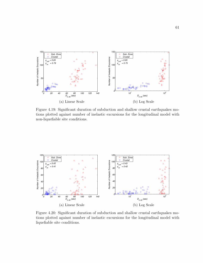
61

0 20 40 60 80 100 120 1400

50

100

150

D5−95

(sec)

Nu

mb

er

of

Ine

lastic E

xcu

rsio

ns

Sub. Zone

Crustal

ρsub

= 0.65

ρsc

= 0.79

101

102

0

50

100

150

D5−95

(sec)

Nu

mb

er

of

Ine

lastic E

xcu

rsio

ns

Sub. Zone

Crustal

ρsub

= 0.65

ρsc

= 0.75


Figure 4.19: Significant duration of subduction and shallow crustal earthquakes motions plotted against number of inelastic excursions for the longitudinal model with non-liquefiable site conditions.

0 20 40 60 80 100 120 1400

20

40

60

80

100

120

D5−95

(sec)

Nu

mb

er

of

Ine

lastic E

xcu

rsio

ns

Sub. Zone

Crustal

ρsub

= 0.45

ρsc

= 0.41

101

102

0

20

40

60

80

100

120

D5−95

(sec)

Nu

mb

er

of

Ine

lastic E

xcu

rsio

ns

Sub. Zone

Crustal

ρsub

= 0.43

ρsc

= 0.42


Figure 4.20: Significant duration of subduction and shallow crustal earthquakes motions plotted against number of inelastic excursions for the longitudinal model with liquefiable site conditions.

62

0 20 40 60 80 100 120 1400

50

100

150

200

250

D5−95

(sec)

Nu

mb

er

of

Ine

lastic E

xcu

rsio

ns

Sub. Zone

Crustal

ρsub

= 0.20

ρsc

= 0.59

101

102

0

50

100

150

200

250

D5−95

(sec)

Nu

mb

er

of

Ine

lastic E

xcu

rsio

ns

Sub. Zone

Crustal

ρsub

= 0.19

ρsc

= 0.60


Figure 4.21: Significant duration of subduction and shallow crustal earthquakes motions plotted against number of inelastic excursions for the transverse model with non-liquefiable site conditions.

0 20 40 60 80 100 120 1400

20

40

60

80

100

120

140

160

180

D5−95

(sec)

Nu

mb

er

of

Ine

lastic E

xcu

rsio

ns

Sub. Zone

Crustal

ρsub

= 0.36

ρsc

= 0.34

101

102

0

20

40

60

80

100

120

140

160

180

D5−95

(sec)

Nu

mb

er

of

Ine

lastic E

xcu

rsio

ns

Sub. Zone

Crustal

ρsub

= 0.35

ρsc

= 0.39


Figure 4.22: Significant duration of subduction and shallow crustal earthquakes motions plotted against number of inelastic excursions for the transverse model with liquefiable site conditions.

63

0 2000 4000 6000 8000 100000

50

100

150

CAV5 (cm/s)

Nu

mb

er

of

Ine

lastic E

xcu

rsio

ns

Sub. Zone

Crustal

ρsub

= 0.48

ρsc

= 0.52

103

0

50

100

150

CAV5 (cm/s)

Nu

mb

er

of

Ine

lastic E

xcu

rsio

ns

Sub. Zone

Crustal

ρsub

= 0.48

ρsc

= 0.56


Figure 4.23: Cumulative absolute velocity five of subduction and shallow crustal earthquakes motions plotted against number of inelastic excursions for the longitudinal model with non-liquefiable site conditions.

0 2000 4000 6000 8000 100000

20

40

60

80

100

120

CAV5 (cm/s)

Nu

mb

er

of

Ine

lastic E

xcu

rsio

ns

Sub. Zone

Crustal

ρsub

= 0.35

ρsc

= 0.15

103

0

20

40

60

80

100

120

CAV5 (cm/s)

Nu

mb

er

of

Ine

lastic E

xcu

rsio

ns

Sub. Zone

Crustal

ρsub

= 0.31

ρsc

= 0.20


Figure 4.24: Cumulative absolute velocity five of subduction and shallow crustal earthquakes motions plotted against number of inelastic excursions for the longitudinal model with liquefiable site conditions.

64

0 2000 4000 6000 8000 100000

50

100

150

200

250

CAV5 (cm/s)

Nu

mb

er

of

Ine

lastic E

xcu

rsio

ns

Sub. Zone

Crustal

ρsub

= 0.25

ρsc

= 0.58

103

0

50

100

150

200

250

CAV5 (cm/s)

Nu

mb

er

of

Ine

lastic E

xcu

rsio

ns

Sub. Zone

Crustal

ρsub

= 0.25

ρsc

= 0.58


Figure 4.25: Cumulative absolute velocity five of subduction and shallow crustal earthquakes motions plotted against number of inelastic excursions for the transverse model with non-liquefiable site conditions.

0 2000 4000 6000 8000 100000

20

40

60

80

100

120

140

160

180

CAV5 (cm/s)

Nu

mb

er

of

Ine

lastic E

xcu

rsio

ns

Sub. Zone

Crustal

ρsub

= 0.51

ρsc

= 0.38

103

0

20

40

60

80

100

120

140

160

180

CAV5 (cm/s)

Nu

mb

er

of

Ine

lastic E

xcu

rsio

ns

Sub. Zone

Crustal

ρsub

= 0.47

ρsc

= 0.39


Figure 4.26: Cumulative absolute velocity five of subduction and shallow crustal earthquakes motions plotted against number of inelastic excursions for the transverse model with liquefiable site conditions.

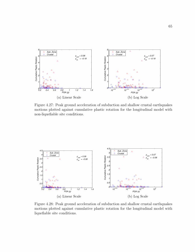
65

0.2 0.4 0.6 0.8 1 1.2 1.4 1.60

1

2

3

4

5

6

PGA (g)

Cu

mu

lative

Pla

stic R

ota

tio

n

Sub. Zone

Crustalρ

sub = 0.08

ρsc

= −0.18

10−0.6

10−0.4

10−0.2

100

0

1

2

3

4

5

6

PGA (g)

Cu

mu

lative

Pla

stic R

ota

tio

n

Sub. Zone

Crustalρ

sub = 0.07

ρsc

= −0.18


Figure 4.27: Peak ground acceleration of subduction and shallow crustal earthquakes motions plotted against cumulative plastic rotation for the longitudinal model with non-liquefiable site conditions.

0.2 0.4 0.6 0.8 1 1.2 1.4 1.60

0.5

1

1.5

2

2.5

3

3.5

4

4.5

PGA (g)

Cu

mu

lative

Pla

stic R

ota

tio

n

Sub. Zone

Crustalρ

sub = 0.09

ρsc

= −0.08

10−0.6

10−0.4

10−0.2

100

0

0.5

1

1.5

2

2.5

3

3.5

4

4.5

PGA (g)

Cu

mu

lative

Pla

stic R

ota

tio

n

Sub. Zone

Crustalρ

sub = 0.07

ρsc

= −0.06


Figure 4.28: Peak ground acceleration of subduction and shallow crustal earthquakes motions plotted against cumulative plastic rotation for the longitudinal model with liquefiable site conditions.

66

0.2 0.4 0.6 0.8 1 1.2 1.4 1.60

0.5

1

1.5

2

2.5

PGA (g)

Cu

mu

lative

Pla

stic R

ota

tio

n

Sub. Zone

Crustalρ

sub = 0.06

ρsc

= 0.00

10−0.6

10−0.4

10−0.2

100

0

0.5

1

1.5

2

2.5

PGA (g)

Cu

mu

lative

Pla

stic R

ota

tio

n

Sub. Zone

Crustalρ

sub = 0.08

ρsc

= 0.01


Figure 4.29: Peak ground acceleration of subduction and shallow crustal earthquakes motions plotted against cumulative plastic rotation for the transverse model with non-liquefiable site conditions.

0.2 0.4 0.6 0.8 1 1.2 1.4 1.60

0.2

0.4

0.6

0.8

1

1.2

1.4

1.6

1.8

PGA (g)

Cu

mu

lative

Pla

stic R

ota

tio

n

Sub. Zone

Crustalρ

sub = 0.00

ρsc

= 0.19

10−0.6

10−0.4

10−0.2

100

0

0.2

0.4

0.6

0.8

1

1.2

1.4

1.6

1.8

PGA (g)

Cu

mu

lative

Pla

stic R

ota

tio

n

Sub. Zone

Crustalρ

sub = −0.01

ρsc

= 0.26


Figure 4.30: Peak ground acceleration of subduction and shallow crustal earthquakes motions plotted against cumulative plastic rotation for the transverse model with liquefiable site conditions.

67

20 40 60 80 100 1200

1

2

3

4

5

6

PGV (cm/s)

Cu

mu

lative

Pla

stic R

ota

tio

n

Sub. Zone

Crustal

ρsub

= 0.74

ρsc

= 0.68

102

0

1

2

3

4

5

6

PGV (cm/s)

Cu

mu

lative

Pla

stic R

ota

tio

n

Sub. Zone

Crustal

ρsub

= 0.70

ρsc

= 0.62


Figure 4.31: Peak ground velocity of subduction and shallow crustal earthquakes motions plotted against cumulative plastic rotation for the longitudinal model with non-liquefiable site conditions.

20 40 60 80 100 1200

0.5

1

1.5

2

2.5

3

3.5

4

4.5

PGV (cm/s)

Cu

mu

lative

Pla

stic R

ota

tio

n

Sub. Zone

Crustal

ρsub

= 0.69

ρsc

= 0.81

102

0

0.5

1

1.5

2

2.5

3

3.5

4

4.5

PGV (cm/s)

Cu

mu

lative

Pla

stic R

ota

tio

n

Sub. Zone

Crustal

ρsub

= 0.64

ρsc

= 0.71


Figure 4.32: Peak ground velocity of subduction and shallow crustal earthquakes motions plotted against cumulative plastic rotation for the longitudinal model with liquefiable site conditions.

68

20 40 60 80 100 1200

0.5

1

1.5

2

2.5

PGV (cm/s)

Cu

mu

lative

Pla

stic R

ota

tio

n

Sub. Zone

Crustal

ρsub

= 0.23

ρsc

= 0.47

102

0

0.5

1

1.5

2

2.5

PGV (cm/s)

Cu

mu

lative

Pla

stic R

ota

tio

n

Sub. Zone

Crustal

ρsub

= 0.20

ρsc

= 0.45


Figure 4.33: Peak ground velocity of subduction and shallow crustal earthquakes motions plotted against cumulative plastic rotation for the transverse model with non-liquefiable site conditions.

20 40 60 80 100 1200

0.2

0.4

0.6

0.8

1

1.2

1.4

1.6

1.8

PGV (cm/s)

Cu

mu

lative

Pla

stic R

ota

tio

n

Sub. Zone

Crustal

ρsub

= 0.41

ρsc

= 0.55

102

0

0.2

0.4

0.6

0.8

1

1.2

1.4

1.6

1.8

PGV (cm/s)

Cu

mu

lative

Pla

stic R

ota

tio

n

Sub. Zone

Crustal

ρsub

= 0.37

ρsc

= 0.51


Figure 4.34: Peak ground velocity of subduction and shallow crustal earthquakes motions plotted against cumulative plastic rotation for the transverse model with liquefiable site conditions.

69

0 5 10 15 200

1

2

3

4

5

6

Ia (m/s)

Cu

mu

lative

Pla

stic R

ota

tio

n

Sub. Zone

Crustal

ρsub

= 0.38

ρsc

= −0.03

100

101

0

1

2

3

4

5

6

Ia (m/s)

Cu

mu

lative

Pla

stic R

ota

tio

n

Sub. Zone

Crustal

ρsub

= 0.32

ρsc

= 0.07


Figure 4.35: Arias intensity of subduction and shallow crustal earthquakes motions plotted against cumulative plastic rotation for the longitudinal model with non-liquefiable site conditions.

0 5 10 15 200

0.5

1

1.5

2

2.5

3

3.5

4

4.5

Ia (m/s)

Cu

mu

lative

Pla

stic R

ota

tio

n

Sub. Zone

Crustal

ρsub

= 0.35

ρsc

= −0.01

100

101

0

0.5

1

1.5

2

2.5

3

3.5

4

4.5

Ia (m/s)

Cu

mu

lative

Pla

stic R

ota

tio

n

Sub. Zone

Crustal

ρsub

= 0.28

ρsc

= 0.06


Figure 4.36: Arias intensity of subduction and shallow crustal earthquakes motions plotted against cumulative plastic rotation for the longitudinal model with liquefiable site conditions.

70

0 5 10 15 200

0.5

1

1.5

2

2.5

Ia (m/s)

Cu

mu

lative

Pla

stic R

ota

tio

n

Sub. Zone

Crustal

ρsub

= 0.19

ρsc

= 0.15

100

101

0

0.5

1

1.5

2

2.5

Ia (m/s)

Cu

mu

lative

Pla

stic R

ota

tio

n

Sub. Zone

Crustal

ρsub

= 0.21

ρsc

= 0.26


Figure 4.37: Arias intensity of subduction and shallow crustal earthquakes motions plotted against cumulative plastic rotation for the transverse model with non-liquefiable site conditions.

0 5 10 15 200

0.2

0.4

0.6

0.8

1

1.2

1.4

1.6

1.8

Ia (m/s)

Cu

mu

lative

Pla

stic R

ota

tio

n

Sub. Zone

Crustal

ρsub

= 0.12

ρsc

= 0.16

100

101

0

0.2

0.4

0.6

0.8

1

1.2

1.4

1.6

1.8

Ia (m/s)

Cu

mu

lative

Pla

stic R

ota

tio

n

Sub. Zone

Crustal

ρsub

= 0.08

ρsc

= 0.24


Figure 4.38: Arias intensity of subduction and shallow crustal earthquakes motions plotted against cumulative plastic rotation for the transverse model with liquefiable site conditions.

71

0.2 0.4 0.6 0.8 1 1.20

1

2

3

4

5

6

Sa(T

1) (g)

Cu

mu

lative

Pla

stic R

ota

tio

n

Sub. Zone

Crustal

ρsub

= 0.08

ρsc

= 0.17

10−0.4

10−0.3

10−0.2

10−0.1

100

0

1

2

3

4

5

6

Sa(T

1) (g)

Cu

mu

lative

Pla

stic R

ota

tio

n

Sub. Zone

Crustal

ρsub

= 0.06

ρsc

= 0.18


Figure 4.39: Spectral Acceleration at T1 of subduction and shallow crustal earthquakes motions plotted against cumulative plastic rotation for the longitudinal model with non-liquefiable site conditions.

0.2 0.4 0.6 0.8 1 1.20

0.5

1

1.5

2

2.5

3

3.5

4

4.5

Sa(T

1) (g)

Cu

mu

lative

Pla

stic R

ota

tio

n

Sub. Zone

Crustal

ρsub

= 0.09

ρsc

= 0.19

10−0.4

10−0.3

10−0.2

10−0.1

100

0

0.5

1

1.5

2

2.5

3

3.5

4

4.5

Sa(T

1) (g)

Cu

mu

lative

Pla

stic R

ota

tio

n

Sub. Zone

Crustal

ρsub

= 0.07

ρsc

= 0.20


Figure 4.40: Spectral Acceleration at T1 of subduction and shallow crustal earthquakes motions plotted against cumulative plastic rotation for the longitudinal model with liquefiable site conditions.

72

0 0.2 0.4 0.6 0.8 1 1.2 1.40

0.5

1

1.5

2

2.5

Sa(T

1) (g)

Cu

mu

lative

Pla

stic R

ota

tio

n

Sub. Zone

Crustal

ρsub

= 0.15

ρsc

= 0.14

10−0.9

10−0.7

10−0.5

10−0.3

10−0.1

0

0.5

1

1.5

2

2.5

Sa(T

1) (g)

Cu

mu

lative

Pla

stic R

ota

tio

n

Sub. Zone

Crustal

ρsub

= 0.17

ρsc

= 0.09


Figure 4.41: Spectral Acceleration at T1 of subduction and shallow crustal earthquakes motions plotted against cumulative plastic rotation for the transverse model with non-liquefiable site conditions.

0 0.2 0.4 0.6 0.8 1 1.2 1.40

0.2

0.4

0.6

0.8

1

1.2

1.4

1.6

1.8

Sa(T

1) (g)

Cu

mu

lative

Pla

stic R

ota

tio

n

Sub. Zone

Crustal

ρsub

= −0.05

ρsc

= 0.16

10−0.9

10−0.7

10−0.5

10−0.3

10−0.1

0

0.2

0.4

0.6

0.8

1

1.2

1.4

1.6

1.8

Sa(T

1) (g)

Cu

mu

lative

Pla

stic R

ota

tio

n

Sub. Zone

Crustal

ρsub

= 0.00

ρsc

= 0.15


Figure 4.42: Spectral Acceleration at T1 of subduction and shallow crustal earthquakes motions plotted against cumulative plastic rotation for the transverse model with liquefiable site conditions.

73

0 20 40 60 80 100 120 1400

1

2

3

4

5

6

D5−95

(sec)

Cu

mu

lative

Pla

stic R

ota

tio

n

Sub. Zone

Crustal

ρsub

= 0.51

ρsc

= 0.21

101

102

0

1

2

3

4

5

6

D5−95

(sec)

Cu

mu

lative

Pla

stic R

ota

tio

n

Sub. Zone

Crustal

ρsub

= 0.47

ρsc

= 0.19


Figure 4.43: Significant duration of subduction and shallow crustal earthquakes motions plotted against cumulative plastic rotation for the longitudinal model with non-liquefiable site conditions.

0 20 40 60 80 100 120 1400

0.5

1

1.5

2

2.5

3

3.5

4

4.5

D5−95

(sec)

Cu

mu

lative

Pla

stic R

ota

tio

n

Sub. Zone

Crustal

ρsub

= 0.42

ρsc

= 0.04

101

102

0

0.5

1

1.5

2

2.5

3

3.5

4

4.5

D5−95

(sec)

Cu

mu

lative

Pla

stic R

ota

tio

n

Sub. Zone

Crustal

ρsub

= 0.38

ρsc

= 0.03


Figure 4.44: Significant duration of subduction and shallow crustal earthquakes motions plotted against cumulative plastic rotation for the longitudinal model with liquefiable site conditions.

74

0 20 40 60 80 100 120 1400

0.5

1

1.5

2

2.5

D5−95

(sec)

Cu

mu

lative

Pla

stic R

ota

tio

n

Sub. Zone

Crustal

ρsub

= 0.35

ρsc

= 0.51

101

102

0

0.5

1

1.5

2

2.5

D5−95

(sec)

Cu

mu

lative

Pla

stic R

ota

tio

n

Sub. Zone

Crustal

ρsub

= 0.35

ρsc

= 0.52


Figure 4.45: Significant duration of subduction and shallow crustal earthquakes motions plotted against cumulative plastic rotation for the transverse model with non-liquefiable site conditions.

0 20 40 60 80 100 120 1400

0.2

0.4

0.6

0.8

1

1.2

1.4

1.6

1.8

D5−95

(sec)

Cu

mu

lative

Pla

stic R

ota

tio

n

Sub. Zone

Crustal

ρsub

= 0.45

ρsc

= 0.26

101

102

0

0.2

0.4

0.6

0.8

1

1.2

1.4

1.6

1.8

D5−95

(sec)

Cu

mu

lative

Pla

stic R

ota

tio

n

Sub. Zone

Crustal

ρsub

= 0.43

ρsc

= 0.30


Figure 4.46: Significant duration of subduction and shallow crustal earthquakes motions plotted against cumulative plastic rotation for the transverse model with liquefiable site conditions.

75

0 2000 4000 6000 8000 100000

1

2

3

4

5

6

CAV5 (cm/s)

Cu

mu

lative

Pla

stic R

ota

tio

n

Sub. Zone

Crustal

ρsub

= 0.48

ρsc

= 0.15

102

103

104

0

1

2

3

4

5

6

CAV5 (cm/s)

Cu

mu

lative

Pla

stic R

ota

tio

n

Sub. Zone

Crustal

ρsub

= 0.40

ρsc

= 0.17


Figure 4.47: Cumulative absolute velocity five of subduction and shallow crustal earthquakes motions plotted against cumulative plastic rotation for the longitudinal model with non-liquefiable site conditions.

0 2000 4000 6000 8000 100000

0.5

1

1.5

2

2.5

3

3.5

4

4.5

CAV5 (cm/s)

Cu

mu

lative

Pla

stic R

ota

tio

n

Sub. Zone

Crustal

ρsub

= 0.43

ρsc

= 0.07

102

103

104

0

0.5

1

1.5

2

2.5

3

3.5

4

4.5

CAV5 (cm/s)

Cu

mu

lative

Pla

stic R

ota

tio

n

Sub. Zone

Crustal

ρsub

= 0.35

ρsc

= 0.09


Figure 4.48: Cumulative absolute velocity five of subduction and shallow crustal earthquakes motions plotted against cumulative plastic rotation for the longitudinal model with liquefiable site conditions.

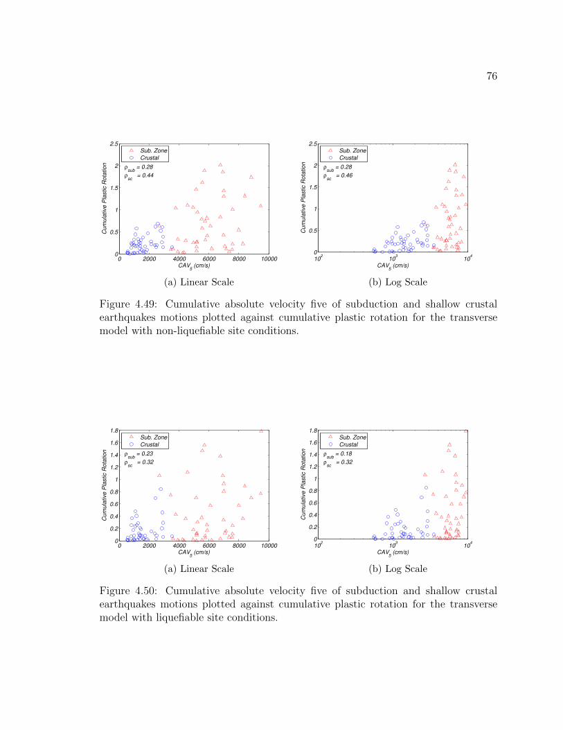
76

0 2000 4000 6000 8000 100000

0.5

1

1.5

2

2.5

CAV5 (cm/s)

Cu

mu

lative

Pla

stic R

ota

tio

n

Sub. Zone

Crustal

ρsub

= 0.28

ρsc

= 0.44

102

103

104

0

0.5

1

1.5

2

2.5

CAV5 (cm/s)

Cu

mu

lative

Pla

stic R

ota

tio

n

Sub. Zone

Crustal

ρsub

= 0.28

ρsc

= 0.46


Figure 4.49: Cumulative absolute velocity five of subduction and shallow crustal earthquakes motions plotted against cumulative plastic rotation for the transverse model with non-liquefiable site conditions.

0 2000 4000 6000 8000 100000

0.2

0.4

0.6

0.8

1

1.2

1.4

1.6

1.8

CAV5 (cm/s)

Cu

mu

lative

Pla

stic R

ota

tio

n

Sub. Zone

Crustal

ρsub

= 0.23

ρsc

= 0.32

102

103

104

0

0.2

0.4

0.6

0.8

1

1.2

1.4

1.6

1.8

CAV5 (cm/s)

Cu

mu

lative

Pla

stic R

ota

tio

n

Sub. Zone

Crustal

ρsub

= 0.18

ρsc

= 0.32


Figure 4.50: Cumulative absolute velocity five of subduction and shallow crustal earthquakes motions plotted against cumulative plastic rotation for the transverse model with liquefiable site conditions.

77

Table 4.1: Correlation coefficients for the longitudinal model with subduction zone ground motions

Subduction Zone Earthquakes Longitudinal Model NIE CPR Peak θ ln| Peak θ| Residual θ

NL Liq NL Liq NL Liq NL Liq NL Liq PGA

ln| PGA|PGV

ln|PGV|Ia

ln| Ia|Sa(T1)

ln|Sa(T1)|D5−95

ln| D5−95|CAV5

ln|CAV5|

-0.07 -0.08 0.57 0.58 0.32 0.34 0.18 0.20 0.65 0.65 0.48 0.48

-0.06 -0.05 0.71 0.72 0.22 0.20 0.23 0.24 0.45 0.43 0.35 0.31

0.08 0.07 0.74 0.70 0.38 0.32 0.08 0.06 0.51 0.47 0.48 0.40

0.09 0.07 0.69 0.64 0.35 0.28 0.09 0.07 0.42 0.38 0.43 0.35

-0.05 -0.06 0.80 0.78 0.36 0.31 0.20 0.21 0.49 0.45 0.47 0.40

-0.04 -0.06 0.82 0.80 0.37 0.32 0.22 0.22 0.46 0.42 0.47 0.41

-0.05 -0.06 0.80 0.78 0.36 0.31 0.19 0.19 0.49 0.45 0.47 0.40

-0.04 -0.06 0.82 0.80 0.37 0.32 0.21 0.21 0.46 0.42 0.47 0.41

0.14 0.17 0.08 0.11 0.16 0.19 0.29 0.26 -0.11 -0.08 0.12 0.16

0.05 0.09 0.01 0.04 0.08 0.15 0.20 0.17 -0.11 -0.09 0.06 0.12

NIE

θ - Relative Deck Drift

NL - Non-liquefiable Soil; Liq - Liquefiable Soil

- Number of Inelastic Excursions; CPR - Cumulative Plastic Rotation

78

Table 4.2: Correlation coefficients for the longitudinal model with shallow crustal ground motions

Shallow Crustal Earthquakes Longitudinal Model NIE CPR Peak θ ln| Peak θ| Residual θ


ln| PGA|PGV

ln|PGV|Ia

ln| Ia|Sa(T1)

ln|Sa(T1)|D5−95

ln| D5−95|CAV5

ln|CAV5|

-0.24 -0.28 -0.23 -0.22 0.07 0.24 0.21 0.21 0.79 0.75 0.52 0.56

-0.35 -0.40 0.35 0.37 -0.12 -0.06 0.23 0.26 0.41 0.42 0.15 0.20

-0.18 -0.18 0.68 0.62 -0.03 0.07 0.17 0.18 0.21 0.19 0.15 0.17

-0.08 -0.06 0.81 0.71 -0.01 0.06 0.19 0.20 0.04 0.03 0.07 0.09

-0.12 -0.09 0.84 0.75 -0.08 -0.01 0.05 0.04 0.00 0.02 -0.02 0.02

-0.10 -0.08 0.86 0.77 -0.05 0.00 0.05 0.04 -0.01 0.01 -0.01 0.02

-0.23 -0.22 0.79 0.75 -0.14 -0.07 0.12 0.12 0.14 0.17 0.00 0.05

-0.17 -0.18 0.81 0.79 -0.07 -0.04 0.10 0.09 0.13 0.15 0.03 0.06

-0.01 -0.03 -0.53 -0.43 0.04 0.04 0.02 0.06 0.27 0.29 0.17 0.15

-0.02 -0.04 -0.57 -0.46 0.05 0.04 -0.03 0.00 0.27 0.29 0.17 0.15



NIE - Number of Inelastic Excursions; CPR - Cumulative Plastic Rotation

79

Table 4.3: Correlation coefficients for the transverse model with subduction zone ground motions

Subduction Zone Earthquakes Transverse Model NIE CPR Peak θ ln| Peak θ| Residual θ


ln| PGA|PGV

ln|PGV|Ia

ln| Ia|Sa(T1)

ln|Sa(T1)|D5−95

ln| D5−95|CAV5

ln|CAV5|

0.08 0.09 0.47 0.48 0.18 0.19 0.17 0.16 0.20 0.19 0.25 0.25

0.19 0.18 0.52 0.51 0.46 0.42 -0.02 0.02 0.36 0.35 0.51 0.47

0.06 0.08 0.23 0.20 0.19 0.21 0.15 0.17 0.35 0.35 0.28 0.28

0.00 -0.01 0.41 0.37 0.12 0.08 -0.05 0.00 0.45 0.43 0.23 0.18

-0.02 -0.04 0.80 0.78 0.35 0.31 0.38 0.43 0.40 0.37 0.44 0.40

-0.06 -0.08 0.84 0.80 0.42 0.38 0.43 0.49 0.59 0.55 0.55 0.50

-0.02 -0.04 0.80 0.78 0.35 0.31 0.44 0.50 0.40 0.37 0.44 0.40

-0.06 -0.08 0.84 0.80 0.42 0.38 0.51 0.59 0.59 0.55 0.55 0.50

0.19 0.18 0.16 0.18 0.25 0.20 0.23 0.26 -0.13 -0.12 0.18 0.16

0.20 0.19 0.13 0.16 0.25 0.21 0.18 0.20 -0.12 -0.12 0.17 0.16

NIE




80

Table 4.4: Correlation coefficients for the transverse model with shallow crustal ground motions

Shallow Crustal Earthquakes Transverse Model NIE CPR Peak θ ln| Peak θ| Residual θ


ln| PGA|PGV

ln|PGV|Ia

ln| Ia|Sa(T1)

ln|Sa(T1)|D5−95

ln| D5−95|CAV5

ln|CAV5|

-0.13 -0.13 0.27 0.17 0.25 0.37 0.28 0.32 0.59 0.60 0.58 0.58

0.00 0.05 0.57 0.45 0.17 0.27 0.50 0.48 0.34 0.39 0.38 0.39

0.00 0.01 0.47 0.45 0.15 0.26 0.14 0.09 0.51 0.52 0.44 0.46

0.19 0.26 0.55 0.51 0.16 0.24 0.16 0.15 0.26 0.30 0.32 0.32

0.10 0.14 0.76 0.66 0.16 0.21 0.04 0.09 0.05 0.10 0.22 0.22

0.12 0.17 0.77 0.66 0.16 0.21 -0.02 0.04 0.02 0.07 0.20 0.20

0.07 0.09 0.76 0.72 0.17 0.23 0.16 0.19 0.24 0.31 0.29 0.33

0.14 0.18 0.76 0.71 0.19 0.25 -0.01 0.05 0.16 0.25 0.27 0.31

-0.12 -0.15 -0.46 -0.39 -0.19 -0.21 0.01 -0.02 -0.01 -0.05 -0.22 -0.20

-0.06 -0.10 -0.74 -0.59 -0.03 -0.07 0.01 -0.04 0.06 0.05 -0.04 -0.04

NIE




81

Table 4.5: Number of inelastic excursions observed for crustal motions

Shallow Crustal Motions Motion # L-NL L-Liq T -NL T-Liq

NIE CPR PθR NIE CPR PθR NIE CPR PθR NIE CPR PθR 1 27 1.77 3.96 22 0.75 3.89 25 0.69 7.31 * * * 2 14 0.06 1.51 3 0.01 1.33 6 0.19 1.80 7 0.08 1.76 3 13 0.29 4.25 7 0.05 4.14 9 0.25 2.30 9 0.18 2.27 4 13 0.05 1.66 1 0 1.73 14 0.22 3.71 10 0.16 3.64 5 19 0.15 2.59 13 0.07 2.70 14 0.19 3.85 12 0.25 3.82 6 1 0 1.01 1 0 1.04 11 0.22 4.54 5 0.36 4.50 7 6 1.32 12.96 9 1.25 13.22 33 0.44 19.73 39 0.48 23.30 8 6 0.02 1.12 1 0 1.55 5 0.01 0.97 3 0 0.94 9 15 0.08 1.66 3 0.01 1.84 6 0.03 1.91 5 0.02 1.87 10 18 0.08 1.66 1 0 1.73 14 0.21 3.17 10 0.12 3.13 11 7 0.03 1.69 3 0.01 1.94 6 0.02 1.22 4 0 1.19 12 10 0.03 1.22 3 0.01 1.73 6 0.15 2.45 8 0.07 2.45 13 11 0.2 1.84 5 0.01 1.98 4 0.02 1.73 6 0.02 1.69 14 9 0.14 2.66 10 0.11 2.66 13 0.12 2.70 9 0.09 2.66 15 9 0.03 1.19 1 0 1.19 14 0.02 1.08 15 0.03 1.08 16 6 0.03 1.69 8 0.03 1.76 6 0.14 1.44 12 0.08 1.44 17 20 0.33 3.24 19 0.09 3.53 15 0.06 2.48 10 0.03 2.48 18 4 0.04 2.09 5 0.01 2.12 8 0.03 1.84 6 0.02 1.84 19 15 0.23 2.63 8 0.14 2.56 9 0.33 2.38 11 0.09 2.34 20 18 0.07 1.66 3 0 1.62 11 0.62 4.61 10 0.69 4.61 21 26 0.13 1.48 5 0 1.66 35 0.15 1.58 11 0.03 1.58 22 13 0.06 1.40 5 0.01 1.37 14 0.22 2.27 8 0.05 2.30 23 7 0.05 1.76 4 0.01 2.16 34 0.38 5.55 12 0.29 5.47 24 14 0.1 2.66 4 0.06 3.02 14 0.2 3.06 * * * 25 27 0.22 2.92 15 0.1 2.56 24 0.47 3.93 12 0.09 3.06 26 11 0.04 1.15 1 0 1.22 9 0.1 2.38 11 0.08 2.34 27 16 0.26 3.78 7 0.07 3.89 18 0.29 3.20 19 0.12 3.20 28 22 0.13 1.26 7 0.02 1.12 14 0.31 1.48 * * * 29 19 0.53 4.03 12 0.21 4.36 21 0.38 5.58 12 0.18 1.44 30 14 0.07 2.45 4 0.01 2.52 14 0.33 7.24 9 0.29 7.20 31 8 1.37 10.23 6 0.97 9.90 9 0.58 9.11 10 0.41 9.18 32 10 0.03 1.19 2 0 1.19 4 0 0.90 4 0 0.83 33 17 0.04 1.37 2 0 1.26 12 0.04 1.08 11 0.03 1.12 34 18 0.05 1.62 3 0 1.69 15 0.27 2.52 19 0.2 2.56 35 7 0.02 1.33 1 0 1.33 13 0.07 1.55 10 0.05 1.55 36 6 0.02 1.19 1 0 1.15 8 0.04 1.51 4 0.02 1.51 37 11 0.03 1.84 2 0.01 1.80 3 0.01 1.37 2 0 1.37 38 10 0.36 4.18 13 0.14 4.32 10 0.24 4.14 18 0.21 4.14 39 15 0.08 1.51 1 0 1.30 22 0.1 1.58 9 0.02 1.55 40 13 0.06 1.62 3 0.01 1.51 7 0.01 1.22 * * * 41 30 0.89 3.67 22 0.17 3.42 28 0.28 1.80 5 0.01 1.19 42 8 0.26 3.28 10 0.05 3.24 10 0.24 2.45 10 0.26 2.45 43 14 0.08 1.37 2 0.01 1.62 11 0.2 1.73 10 0.02 1.73 44 17 0.06 2.05 8 0.01 2.12 19 0.61 3.67 22 0.46 3.64 45 29 0.08 1.04 1 0 1.22 25 0.16 1.40 17 0.07 1.37 46 12 0.06 1.33 4 0 1.55 13 0.18 3.64 12 0.24 3.64 47 7 0.03 1.40 2 0 1.15 23 0.17 3.35 13 0.08 3.35 48 10 1.2 8.28 18 0.89 8.21 28 0.52 35.36 30 0.85 37.77

L - longitudinal Model; T - Transverse Model NL - Non-liquefiable Soil; Liq - Liquefiable Soil

NIE - Number of Inelastic Excursions; CPR - Cumulative Plastic Rotation * Motion did not converge ; PθR - Peak Deck Drift Ratio

82

Table 4.6: Number of inelastic excursions observed for subduction zone motions

Subduction Zone Motions Motion # L-NL L-Liq T -NL T-Liq

NIE CPR PθR NIE CPR PθR NIE CPR PθR NIE CPR PθR 1 28 0.08 2.23 12 0.02 2.23 22 0.05 1.66 6 0.01 1.66 2 113 0.5 2.88 103 0.47 2.66 56 0.74 2.12 22 0.08 2.05 3 66 1.52 4.25 77 0.4 4.25 61 0.34 3.28 * * 4.65 4 56 2.58 6.09 48 2.16 6.12 123 0.3 4.57 91 0.36 1.33 5 46 0.15 2.09 3 0.01 2.12 68 0.31 1.33 48 0.04 2.66 6 66 0.28 2.41 15 0.06 2.56 47 0.15 2.70 59 0.11 0.86 7 39 0.61 1.22 1 0 1.12 52 0.64 0.86 28 1.06 0.94 8 24 0.05 1.04 1 0 1.30 23 0.07 0.97 3 0 1.94 9 57 0.17 2.95 36 0.8 2.92 114 1.03 1.91 102 0.42 2.27 10 82 0.45 2.27 39 0.19 2.52 67 0.22 2.30 71 0.25 1.01 11 21 0.05 1.40 1 0 1.22 13 0.02 1.01 12 0.02 1.87 12 121 0.59 2.66 12 0.08 2.88 73 0.11 1.94 75 0.15 2.45 13 103 0.66 3.20 54 0.28 3.46 83 1.62 2.41 72 1.46 1.19 14 37 0.1 1.19 1 0 1.30 18 0.03 1.19 * * * 15 79 1.23 3.06 33 0.11 3.20 83 1.43 2.16 97 0.93 2.20 16 78 0.34 2.63 40 0.12 3.13 43 0.17 2.23 24 0.13 2.20 17 78 1.11 2.23 73 0.67 2.56 68 1.1 2.56 73 1.12 2.63 18 54 0.22 2.63 10 0.05 2.74 61 0.84 2.09 11 0.03 2.05 19 50 0.41 2.77 48 0.19 3.35 217 0.81 2.34 63 0.26 2.30 20 53 0.19 1.48 3 0 1.40 53 0.1 1.33 38 0.05 1.37 21 57 0.22 1.91 5 0.01 1.80 49 1.89 2.41 57 1.56 2.41 22 73 0.26 2.23 36 0.08 2.12 84 0.43 1.69 103 0.34 1.66 23 37 0.14 1.62 4 0 1.76 99 0.78 1.30 115 0.38 1.30 24 46 0.11 1.12 1 0 1.33 * * * 9 0.01 0.94 25 147 2.26 4.86 110 0.85 4.65 83 0.12 0.97 133 0.89 4.65 26 99 5.63 7.92 79 3.54 7.17 97 1.31 4.54 109 1.79 6.09 27 98 0.84 2.77 46 0.17 2.56 77 0.25 1.91 43 0.18 1.91 28 106 0.78 3.06 53 0.24 3.20 66 0.26 2.41 32 0.09 2.38 29 47 0.14 1.12 2 0 1.15 65 0.58 0.97 12 0.01 0.97 30 56 0.24 2.92 15 0.07 2.74 69 0.23 2.09 106 0.36 2.05 31 80 0.36 2.16 21 0.09 2.34 63 2.01 2.45 137 1.38 2.41 32 87 2.46 4.93 93 0.95 4.39 98 1.74 3.38 164 0.7 3.35 33 37 0.08 1.30 7 0.01 1.40 37 0.94 1.30 62 0.3 1.26 34 36 0.12 1.94 7 0.03 2.23 43 0.04 1.30 54 0.06 1.22 35 45 0.11 1.12 1 0 1.33 56 1.05 1.01 11 0.01 1.01 36 61 0.24 3.10 41 0.07 3.31 82 1.01 3.13 42 0.11 3.10 37 95 4.24 5.11 67 3.46 5.83 100 1.09 5.04 114 0.76 5.01 38 83 5.74 7.63 77 4.16 7.06 110 0.55 4.25 118 0.58 4.29 39 48 0.2 2.59 10 0.05 2.63 52 0.1 2.27 73 0.74 2.20 40 78 0.34 2.81 27 0.06 2.70 74 0.27 2.09 45 0.12 2.05 41 106 0.5 3.06 83 0.59 3.24 110 0.41 2.38 74 0.17 2.38 42 86 0.42 3.02 23 0.1 2.92 70 1.47 2.52 98 0.7 2.45 43 115 0.75 2.88 51 0.19 2.63 89 1.3 2.45 73 0.81 2.41 44 97 2.82 3.78 103 1.37 3.93 141 1.85 3.71 58 1.06 3.78 45 43 1.73 3.10 58 0.87 3.31 93 0.11 1.73 20 0.04 1.84 46 49 1.29 3.02 13 0.02 2.81 59 0.64 2.52 118 0.58 2.45

L - longitudinal Model; T - Transverse Model NL - Non-liquefiable Soil; Liq - Liquefiable Soil

NIE - Number of Inelastic Excursions; CPR - Cumulative Plastic Rotation * Motion did not converge ; PθR - Peak Deck Drift Ratio

83

Table 4.7: Summary table of NIE and CPR for shallow crustal earthquakes

Shallow Crustal Earthquakes

Mean Median Std. Div

L-NL L-Liq T-NL T-Liq NIE CPR NIE CPR NIE CPR NIE CPR 14 13 7

0.23 0.08 0.39

6 4 6

0.11 0.01 0.27

14 13 8

0.22 0.20 0.18

11 10 7

0.16 0.08 0.19

L - longitudinal Model; T - Transverse Model



Table 4.8: Summary table of NIE and CPR for subduction zone earthquakes

Subduction Zone Earthquakes

Mean Median Std. Div

L-NL L-Liq T-NL T-Liq NIE CPR NIE CPR NIE CPR NIE CPR 69 64 29

0.94 0.39 1.34

36 30 32

0.49 0.09 0.95

74 68 35

0.68 0.55 0.58

65 63 41

0.46 0.28 0.48

L - longitudinal Model; T - Transverse Model



84

Figures 4.3 to 4.26 show that subduction zone motions cause significantly greater

numbers of inelastic excursions (NIE) and cumulative plastic rotations (CPR) com

pared to shallow crustal motions. The increases in the NIE and CPR for the sub

duction ground motions occurred for both bridge orientations (i.e., longitudinal or

transverse) an for both site-soil conditions (liquefiable, or non-liquefiable). The larger

NIE and CPR for the subduction zone motions suggest that an increase in ground

motion duration does increase unrecoverable plastic deformations.

The correlation of the NIE and CPR with increasing ground motion intensity is

much more robust for intensity measures that consider duration. Accordingly, PGA,

PGV, Sa(T 1), and Ia do not accurately predict the NIE and CPR Figure 4.3 shows

that an earthquake motion with a PGA of 0.4 g could produce approximately 10

to 100 inelastic excursions. CAV5, which incorporate ground motion duration and

amplitudinal intensity, predicts the NIE and CPR with increasing ground motion

intensity much more robustly. For instance, a CAV5 of 5000 cm/s (Figure 4.23)

predicts the number of inelastic excursions to be between 25 and 75. Correlation

coefficients reported in Tables 4.1 to 4.4 were calculated for each combination of

ground type, modal configuration, site-soil condition, and assume normal and log

normal distribution of data.

The average number of inelastic excursions for the transverse model is slightly

higher than the longitudinal model for identical site-soil conditions. The recorded

data for the transverse model also has greater dispersion compared to longitudinal

model. These two trends are observed for both liquefiable and non-liquefiable site-soil

conditions. The higher damage in the transverse model is possibly caused by the lack

of fixity at the bridge deck, which is provided in the longitudinal model by the bridge

abutments.

The liquefiable site-soil conditions produced lower NIE and CPR compared to the

85

non-liquefiable conditions. The lower superstructure demands can be observed for the

both transverse and longitudinal models. A potential reason for the lower superstruc

ture demand for bridges atop liquefiable layers is that earthquake motion has been

altered. When an earthquake motion propagates through a liquefiable layer, the fun

damental properties of the motion (i.e. frequency content and intensity) are altered

(Kramer 1996). For the soil-bridge model and site-soil conditions model herein, the

changed motions decreases superstructure demands. It is important to note that with

different models, and soil profiles, the liquefiable layer may increase superstructure

demands.

The shallow crustal earthquake motion with the PGA of 1.3 g illustrated in Fig

ures 4.3, 4.4, 4.5, and 4.6 is the UC Santa Cruz (UCSC) ground motion recording

(motion 11 in Appendix B) of the 1989 Loma Prieta earthquake. The scaled PGA

of 1.3 g may seem unrealistic, but it illustrates the importance of earthquake motion

duration. The UCSC ground motion has the highest PGA of the all the earthquake

motions considered, and typically would not be used for seismic design because of

the exceptionally high PGA. Figure 4.3 illustrates that amplitudinal intensity (e.g.

PGA) of an earthquake motion is not the best indicator of durational damage. A

shallow crustal earthquake motion with a PGA of 0.3 g in Figures 4.3 and 4.27 has

the potential to have twice the NIE and CPR compared with the UCSC motion. The

lack compatibility between the NIE and CPR with increasing amplitudinal intensity

is demonstrated with the UCSC ground motion.

86

Chapter 5: Tsunami Analysis of the Fluid-Soil-Bridge System

This chapter present a multi-hazard framework that evaluates the ability of the

transverse fluid-soil-bridge model with non-liquefiable site-soil conditions to resist

tsunami forces after an earthquake has occurred. The transverse fluid-soil-bridge

model, which was designed for seismically-induced lateral forces, is unlikely to have

sufficient strength, because hydrodynamic tsunami loading was not considered dur

ing the original design. The modeled tsunami loads are representative of the differing

tsunamis that can be expected along the Oregon coast.

The analysis of the transverse fluid-soil-bridge model utilized two separate meth

ods for calculating tsunami loads. First, the Particle Finite Element Method (PFEM)

simulates fluid-structure-interaction (FSI) problems by creating a large fluid domain

with particles bounded by cells. The particles are assigned velocity, mass, and body

forces to simulate fluid properties. The PFEM procedure was used to simulate a

bore. Second, FEMA P-646 (2008) was used to apply forces to the fluid-soil-bridge

model simulating tiered tsunami attacks. The computed hydrodynamic forces are

assumed to act in a quasi-steady state and changes in the inundating velocity and

depth changes occur over a long period of time.

5.1 Framework Steps

The transverse fluid-soil-bridge model was selected over the longitudinal model, be

cause it is assumed the exterior area of the bridge deck is orthogonal to the tsunami

wave, such as the Otsuchi Railroad Bridge and Rikuzentakata Automobile Bridge

87

presented in the literature review. Figure 5.1 shows the transverse fluid-soil-bridge

model and the assumed direction of tsunami inundation.

The boundary conditions for the fluid-soil-bridge system were originally devel

oped for the application ground motions as described in Chapter 3. The boundary

conditions needed to be altered for the tsunami loading. Originally, the fluid-soil

bridge system had no lateral constraints, because the far-field soil-column and pile

were modeled on rollers for the force-dashpot couple at the soil-bedrock interface.

Without lateral constraint and with relatively slow hydrodynamic loading however,

the fluid-soil-bridge system experiences rigid body translation. To prevent uncon

strained rigid body translation, the 9 node “u-p” quadrilateral soil elements were

removed, and the one-dimensional soil interface springs formerly attached to the soil

elements were fixed. Additionally, the force-dashpot couple was removed as it is no

longer required for the hydrodynamic tsunami analysis. Once the required boundary

condition changes were made, a ten second critically damped analysis was performed

to remove any remaining vibrations that were present in the numerical model due to

the earthquake motion. Critical damping was achieved by increasing the Newmark

time integration parameters to 1.5 and 1.0 for β and γ, respectively.

5.2 PFEM Procedure

The PFEM numerical wave flume is 90 m long on the seaside and 30 m on the landside

of the transverse fluid-soil-bridge model. The 90 m flume length to the seaside of the

fluid-soil-bridge model was selected so that an idealized bore would maintain its shape

and velocity throughout the analysis duration. It is that assumed the wave flume is

an impenetrable fixed boundary and vertical loads from the fluid are not transmitted

to the soil. A fixed flume boundary is required for the PFEM procedure in OpenSees.

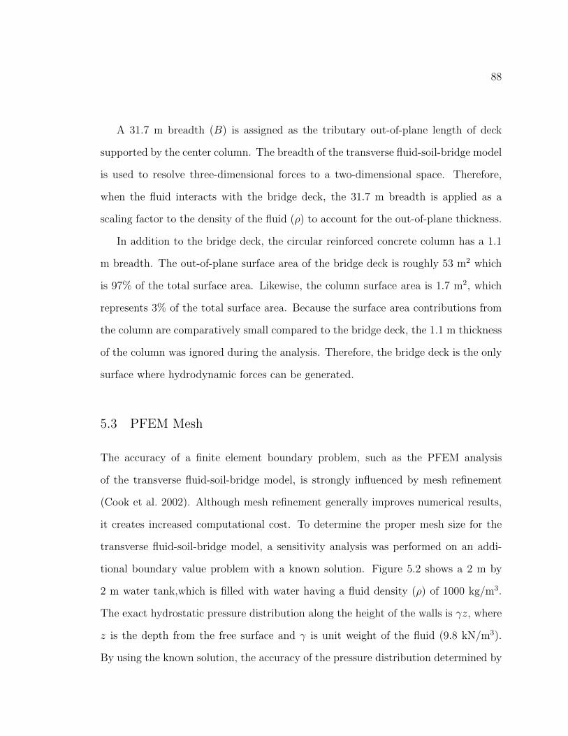
88

A 31.7 m breadth (B) is assigned as the tributary out-of-plane length of deck

supported by the center column. The breadth of the transverse fluid-soil-bridge model

is used to resolve three-dimensional forces to a two-dimensional space. Therefore,

when the fluid interacts with the bridge deck, the 31.7 m breadth is applied as a

scaling factor to the density of the fluid (ρ) to account for the out-of-plane thickness.

In addition to the bridge deck, the circular reinforced concrete column has a 1.1

m breadth. The out-of-plane surface area of the bridge deck is roughly 53 m2 which

is 97% of the total surface area. Likewise, the column surface area is 1.7 m2, which

represents 3% of the total surface area. Because the surface area contributions from

the column are comparatively small compared to the bridge deck, the 1.1 m thickness

of the column was ignored during the analysis. Therefore, the bridge deck is the only

surface where hydrodynamic forces can be generated.

5.3 PFEM Mesh

The accuracy of a finite element boundary problem, such as the PFEM analysis

of the transverse fluid-soil-bridge model, is strongly influenced by mesh refinement

(Cook et al. 2002). Although mesh refinement generally improves numerical results,

it creates increased computational cost. To determine the proper mesh size for the

transverse fluid-soil-bridge model, a sensitivity analysis was performed on an addi

tional boundary value problem with a known solution. Figure 5.2 shows a 2 m by

2 m water tank,which is filled with water having a fluid density (ρ) of 1000 kg/m3 .

The exact hydrostatic pressure distribution along the height of the walls is γ z, where

z is the depth from the free surface and γ is unit weight of the fluid (9.8 kN/m3).

By using the known solution, the accuracy of the pressure distribution determined by

89

Figure

5.1: Con

ceptual

drawing of

the numerical

waveflume an

d idealized

bore with

critical dim

ension

s labeled

(i.e.

h1

, h

0 , and

η).

Soil an

d pile-foundation

not

show

n for

clarity

(Carey

et al. 2014).

90

the PFEM analysis with differing mesh sizes can be determined. It is assumed that

the sensitivity results for this static boundary problem are representative for the bore

analysis. The numerical accuracy versus computational cost curve, generated for the

water tank problem, is assumed to “scaled up” to the fluid-soil-bridge model.

Figure 5.2: 2 m x 2 m static fluid tank used to illustrate mesh refinement

Table 5.1 reports the differing mesh sizes and the respective element domains that

were included for the sensitivity analysis. To ensure that the fluid particles were

numerically static (i.e., initial vibrations were damped-out), a 1,000 step (Δt = 0.001

sec) analysis was run for each initial particle spacing and the pressure distribution

was recorded at the final step. Computational cost for each mesh size was deter

mined by counting the number of milliseconds it took to reach 1,000 analysis steps.

91

The cumulative absolute error between the PFEM and the closed form solution was

calculated by,

2 m

z = 0

where f is the PFEM pressure calculation at some depth z, and γ is the unit weight

of the fluid. The peak computational cost and cumulative error were normalized and

plotted in Figure 5.3 against the normalized system size, which is height of the water

n

tank over the initial mesh size (2 m/Mesh Size ).

Table 5.1: Number of elements and DOFs with corresponding mesh refinement.

f(z) − γz C umulativeError (5.1)=

γz

Mesh Size (mm) Number Elements Number of DOFs

250 200 125 100 80 62.5 50 40 20 16

230 330 726 1070 1586 2486 3750 5690 21390 32986

576 800 1664 2400 3488 5376 8000 12000 44000 67488

In the end, a 90 mm initial mesh size was selected for the fluid-soil-bridge model.

The 90 mm mesh balanced acceptable cumulative error with realistic computational

time. The 90 mm mesh required 8 days of computational time to complete a 3,000

step analysis with a time step of Δt = 0.001 sec. Any future refinement of the 90 mm

mesh exponentially increases computational time, which is illustrated in Figure 5.3.

92

0 50 100 150 200 250

0.2

0.4

0.60.8

1

Normalized System Size

Com

pu

tational expense n

orm

aliz

ed to p

ea

k e

xpe

nse

0 50 100 150 200 2500

0.2

0.4

0.6

0.8

1

Cu

mula

tive

absolu

te e

rror

no

rmaliz

ed t

o p

eak e

rror

Computational Expense

Cumulative Error

Figure 5.3: Effect of mesh refinement on normalized error (3.4) and normalized computational time (8539 seconds).

93

5.3.1 Idealized Bore

An idealized bore was used to represent tsunami wave run-up and is illustrated in

Figure 5.1. Numeric hydrodynamic analysis allows for many potential shapes of

initial bores or waves. The bore shape that was selected to best emulate physical

conditions is a hyperbolic tangent (Yeh et al. 1989; Mohamed 2008). The creation

of a hyperbolic tangent bore required novel scripting in OpenSees, which balanced

computational cost, representation of physical conditions, and limitations of fluid

region shapes that can be discretized in OpenSees.

24 bores with differing initial heights and velocities were created for modeling

tsunami wave interaction with the transverse fluid-soil-bridge model. To maintain

constant initial energy for each of the 24 bores, the Froude number, was held constant

at 1.43 (Yeh et al. 1989). The Froude number, F is given by,

F = 1.43 = √ u0

(5.2)gh0

where h0 is the initial height and u0 is the bore velocity. To create the 24 tsunami

bores, the height h0 was increased by 0.125 m increments and the velocity u0 was

back calculated using Equation 5.2.

The 24 idealized bores do not consider the expected return period of the PNW

tsunami. The bore sizes were selected to generically illustrate how hydrodynamic

tsunami forces affect the fluid-soil-bridge model, and therefore, do not correspond to

a specific design event.

Yeh et al. (1989) suggested that the ratio of the bore height (h0) and hydrostatic

fluid height (h1) over which the bore is traveling be maintained within the range

of 2.0<h1/h0<2.6. Herein h1/h0 was constrained to 2.3. Table 5.2 shows the bore

characteristics for each of the 24 bores considered.

94

Table 5.2: Tsunami bore characteristics h1, h0, u0, & η seen in Figure 5.1 for each of the 24 tsunami bores considered.

h0/h1=2.3 Bore #

Height of Bore h0 (m)

η (m)

Height Standing h1 (m)

Bore Velocity u0 (m/s)

h0u2 Momentum

Flux (m3/s2)

1 4.75 2.68 2.07 6.30 189 2 4.875 2.76 2.12 6.38 199 3 5 2.83 2.17 6.47 209 4 5.125 2.90 2.23 6.55 220 5 5.25 2.97 2.28 6.62 230 6 5.375 3.04 2.34 6.70 242 7 5.5 3.11 2.39 6.78 253 8 5.625 3.18 2.45 6.86 265 9 5.75 3.25 2.50 6.93 276 10 5.875 3.32 2.55 7.01 289 11 6 3.39 2.61 7.08 301 12 6.125 3.46 2.66 7.16 314 13 6.25 3.53 2.72 7.23 327 14 6.375 3.60 2.77 7.30 340 15 6.5 3.67 2.83 7.37 353 16 6.625 3.74 2.88 7.44 367 17 6.75 3.82 2.93 7.51 381 18 6.875 3.89 2.99 7.58 395 19 7 3.96 3.04 7.65 410 20 7.125 4.03 3.10 7.72 424 21 7.25 4.10 3.15 7.79 439 22 7.375 4.17 3.21 7.85 455 23 7.5 4.24 3.26 7.92 470 24 7.625 4.31 3.32 7.98 486

95

Figure 5.4 shows three different regions of the PFEM fluid domain. Each region

represents a different initial velocity. The velocity of Region 1 is the idealized bore

velocity, which is a function of h0 as determined by the Froude number in Equation 5.2.

Region 2 represents the static fluid; therefore, the fluid in Region 2 has no initial

velocity, which is representative of a coastal river or sand. Finally, Region 3 consists

of a velocity gradient that decreases the fluid velocity from the bore (Region 1) to the

static fluid of Region 2. Region 3 is necessary to also reduces numerical instability

that arises from sudden changes in initial velocity along the wave flume.

Figure 5.4: Detailed schematic of the three velocity regions of the PFEM model (i.e idealized bore, standing fluid and transition region).

Notably, tsunami run-up was considered during modeling. Tsunami run-out

(drawdown) may produce higher peak flow velocities (Yeh and Mason 2014); however,

the current modeling framework does not support a flow reversal.

The idealized bore creates numerical high frequency noise during initial impact

with the bridge deck, which is an issue often experienced by tsunami modelers ( e.g.,

Azadbakht 2013). The noise can be attributed to the sudden resistance of the bore

contacting the bridge deck.

Correction of the high frequency noise was performed by using a moving mean

of the last 30 pressure time history data points. Thirty pressure time history data

96

points represent 0.03 seconds of analysis time with the given time step Δt = 0.001

sec. A moving mean was selected over other filtering options, such as low pass fil

tering, because it does not require bounding corner frequencies that are arbitrarily

selected (Azadbakht 2013). Once corrected, the pressure distributions were resolved

and combined to develop vertical force, horizontal force and moment-time histories

at the deck-column connection. The force and moment time histories were applied to

the fluid-soil-bridge model using the same Δt = 0.001 sec time step used to record the

pressure time histories. The application of the bore loading occurs at the conclusion

of the tsunamigenic ground motion, which mimics the complete multi-hazard scenario

of a tsunami following a long duration earthquake.

5.4 Steady State Hydrodynamic Forces

Quasi-steady state hydrodynamic forces are characterized by constant fluid velocity

and depth. Although velocity and depth are variant during tsunami inundation (Fritz

et al. 2012), changes occur over many minutes to hours, which supports a steady-state

assumption. The forces generated during hydrodynamic flow are primarily influenced

by the geometry of the submerged object. The steady state hydrodynamic force

presented by FEMA P-646 (2008) is given as,

FD = 1 CDρB(hu2)max (5.3)

2

where CD is the drag coefficient of the enveloped object, ρ is the density of the fluid,

B is the breadth of the object (out-of-plane), and (hu2)max is the maximum expected

momentum flux per unit mass. For this work, the h in the momentum flux equation

is held constant at depths ranging from zero (i.e. ground surface) to the height

97

of the bridge deck (7.77 m). The velocity, u, is varied from zero to 6 m/s, which

is approximately the maximum flow velocity observed at Kesen-numa bay, Japan

during the 2011 Tohoku Tsunami (Fritz et al. 2012). By incrementing the velocity

from zero to the maximum of 6 m/s, the hydrodynamic force is applied as a linear

ramp function. The ramp function reduces non-convergence of the nonlinear solution

algorithm that can arise from the sudden application of extreme loads.

Unlike the PFEM analysis, which could only accommodate one structural width

(B), Equation 5.3 can be evaluated for both the bridge column diameter and the

bridge deck width. The hydrodynamic forces that occur in the bridge column were

resolved to horizontal force and moment-time histories at the ground surface, and

the forces in the bridge deck were applied at the deck-column connection similar to

the PFEM analysis. Uplift forces produced by buoyant forces beneath the deck were

ignored, because they do not exceed the appointed deck gravity loads.

5.5 PFEM Impulsive Forces

The peak horizontal force, vertical force and rotational moment for each of 24 idealized

bores are given in Table 5.3. Figures 5.5 through 5.7 show the resolved horizontal,

and vertical force and moment-time histories at the bridge deck-column connection

for the arbitrary chosen bore 22. Bore 22 has an initial velocity of 7.85 m/s, a bore

height of 7.375 m, and a standing fluid height of 3.21 m. The initial spikes seen in

Figures 5.5, 5.6 and 5.7 at roughly 0.5 sec occurred in 22 of the idealized bores that

contacted the bridge deck (bores 3-24).

The dynamic force and moment time-histories of the 24 idealized tsunami bores

could not be applied to the fluid-soil-bridge model due to the large impulsive force

spikes. The force spikes exceeded the design capacity of the fluid-soil-bridge system,

98

and non-convergence occurred even with an analysis time step of less than Δt = 0.001

sec.

Table 5.3: Peak horizontal force, vertical force, and moment for each of the 24 idealized tsunami bores resolved at the bridge deck-column connection.

Bore Max Uplift Force (kN)

Max Moment (kN*m)

Max Horizontal Force (kN)

1 7 45 93 2 7 47 93 3 22279 73737 93 4 11893 38528 93 5 23202 68628 93 6 38608 89000 93 7 23774 54055 1453 8 24841 47102 1946 9 37880 64394 2134 10 82715 123690 4350 11 159480 161650 7970 12 177290 173520 9445 13 234240 196610 16902 14 231460 199780 11917 15 234630 204910 14987 16 260520 230140 13519 17 246320 208970 16469 18 262810 241180 17973 19 275650 244600 19451 20 246760 266630 80621 21 272730 291310 141430 22 245990 264710 24670 23 224490 263930 28836 24 243050 316310 30746

99

0 0.5 1 1.5 2 2.50

0.5

1

1.5

2

2.5x 10

4

Time (sec)

Ho

rizon

tal F

orc

e (

kN

)

Bore 22

Figure 5.5: Resolved horizontal force time history at the bridge deck-column connection for idealized bore 22.

0 0.5 1 1.5 2 2.50

0.5

1

1.5

2

2.5x 10

5

Time (sec)

Vert

ical F

orc

e (

kN

)

Bore 22

Figure 5.6: Resolved vertical force time history at the bridge deck-column connection for idealized bore 22

100

0 0.5 1 1.5 2 2.5−3

−2.5

−2

−1.5

−1

−0.5

0

0.5x 10

5

Time (sec)

Rota

tio

nal M

om

ent

(kN

*m)

Bore 22

Figure 5.7: Resolved rotational moment time history at the bridge deck-column connection for idealized bore 22.

101

5.6 Quasi-Steady-State Hydrodynamic Forces

To express damage from two subsequent events, Ribeiro et al. (2014) proposed the

development of interaction diagrams. A proposed earthquake-tsunami interaction

diagram is conceptualized in Figure 5.8. The limit-state surface represents the ex

ceedance of a peak observed response for the structural model, such as base shear,

deck drift ratio. For the fluid-soil-bridge model, failure surfaces were generated for

deck drift ratios of 1.5%, 2.5%, 5.0% and 7.5%. Multiple limit-state surfaces were

generated to show the ductility of the fluid-soil-bridge system at failure, and represent

different design scenarios.

Figure 5.8: Conceptualization of earthquake-tsunami interaction diagram, with dots representing unique analysis runs.

The ground motion intensity parameter used to describe the expected demands

to a fluid-soil-bridge system is the spectral acceleration at the fundamental period

(T 1) of the transverse model (1.71 sec), which is expressed as Sa(T 1) (Baker 2007).

102

Sa(T 1) was used to characterize the ground motion intensity along the ordinate of the

earthquake-tsunami interaction diagram. Momentum flux (hu2) is the hydrodynamic

intensity parameter that is commonly used to express the potential forces that an

inundating tsunami with depth (h) and velocity (u) can impose on a body (FEMA

P-646 2008). Momentum flux represents the strength of the tsunami wave along the

abscissa of the earthquake-tsunami interaction diagram.

The construction of the earthquake-tsunami interaction diagram uses the incre

mental dynamic analysis (IDA) framework (Vamvatsikos and Cornell 2002). The

intensity parameters Sa(T 1) and hu2 are linearly scaled along the respective axis

until the predefined limit-state is reached. At each unique combination of spectral

acceleration and tsunami intensity an analysis is required for a total of N number

of analysis, where N is the product (N = NSa(T1) × Nhu2 ) of the number abscissa

increments (NSa(T1)) and the number of ordinate increments (Nhu2 ).

Herein, ten spectral acceleration steps (NSa(T1)=10) and 15 momentum flux steps

(Nhu2 =15) are used; accordingly, for a total of 150 analyses were required to create

the earthquake-tsunami interaction diagram. The construction of the earthquake-

tsunami interaction diagram was repeated for 12 different earthquake motions, which

are reported in Table 5.5. Creating the 12 earthquake-tsunami interaction diagrams

(1800 analyses in total) represented a significant computational effort. The HTCondor

system at Oregon State University allowed for simultaneous analyses and reduced the

total time to create each earthquake-tsunami diagram from days to hours.

The maximum quasi-steady-state hydrodynamic forces applied to the transverse

fluid-soil-bridge model are reported in Table 5.4. With the calculated hydrodynamic

forces in Table 5.4, the earthquake-tsunami interaction diagram could be created as

shown in Figure 5.9 for the FKSH12 fault parallel earthquake motion with a PGA of

0.5 g and a Sa(T 1) of 0.30 g, (see Appendix A).

103

The failure surfaces shown for the earthquake-tsunami interaction diagram in

Figure 5.9 has little to no slope near the ordinate, because expected failure of the fluid

soil-bridge system is controlled by the intensity of the tsunami. When the intensity of

the earthquake motion degrades the strength of fluid-soil-bridge system to the point

where only minimal hydrodynamic tsunami forces can be resisted, the earthquake-

tsunami interaction diagram intersects the abscissa. The abscissa intersection is the

point where the fluid-soil-bridge system is controlled by the intensity of the earthquake

motion.

To understand the tsunami controlled region of the earthquake-tsunami interac

tion diagram, the momentum flux is plotted against the observed deck drift ratio in

Figure 5.10 for the same FKSH12 fault parallel earthquake motion. Although not

shown, the deck drift ratio for each curve plotted in Figure 5.10 reached the failure

state of 7.5% drift. Each line in Figure 5.10 represents a different spectral acceler

ation at Sa(T 1). It can be observed from Figure 5.10 shows that, regardless of the

spectral acceleration of the earthquake motion, the soil bridge system failed at sim

ilar momentum flux values. For the earthquake motion used to create Figure 5.10,

the average hu2 value that resulted in failure is 236.6 m3/s2 . Note that this value is

specific to the examined fluid-soil-bridge model.

Figures 5.9 and 5.10 also show the failure of the fluid-soil-bridge system was non-

ductile. Figure 5.9 shows that a small increase in tsunami loading (hu2) causes the

peak deck drift ratio to change from 1.5% to 7.5%. Figure 5.10 validates the notion

of non-ductile response of the fluid-soil-bridge system with the discontinuity to resist

tsunami loading at roughly 240 m3/s2 .

104

Table 5.4: Quasi-steady-state hydrodynamic forces applied to the transverse fluidsoil-bridge model.

Depth of Fluid (m)

Max CV (kN)

Max CM (kN*m)

Max DV (kN)

Max DM (kN*m)

3 75 113 * * 4 100 200 * * 5 125 313 * * 6 150 451 * *

6.25 153 466 188 14 6.5 153 466 502 100 6.55 153 466 565 127 6.6 153 466 628 157 6.65 153 466 690 190 6.7 153 466 753 226 6.75 153 466 816 265 6.8 153 466 879 308 6.825 153 466 910 330 6.85 153 466 941 353 6.875 153 466 973 377

CV - Column Shear Force DV - Deck Shear Force CM - Column Rotational Moment DM - Deck Rotational Moment

* - Fluid did not reach bridge deck

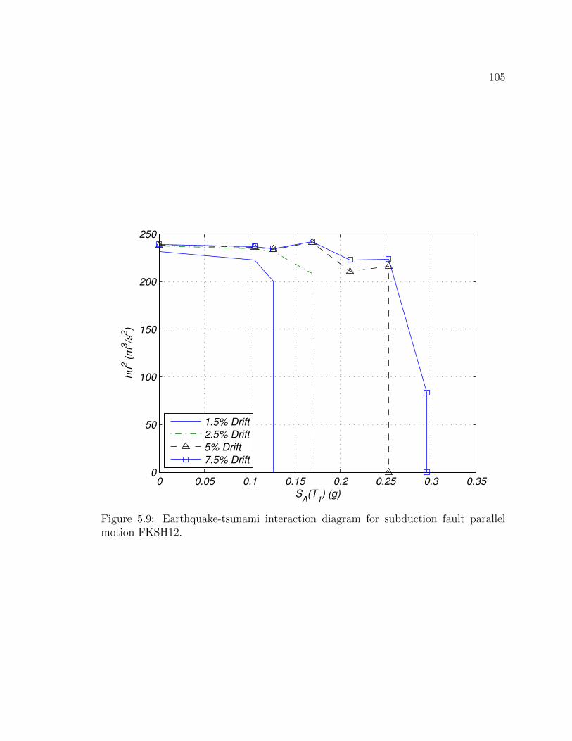
105

0 0.05 0.1 0.15 0.2 0.25 0.3 0.350

50

100

150

200

250

SA(T

1) (g)

hu

2 (

m3/s

2)

1.5% Drift

2.5% Drift

5% Drift

7.5% Drift

Figure 5.9: Earthquake-tsunami interaction diagram for subduction fault parallel motion FKSH12.

106

120 140 160 180 200 220 2400

0.05

0.1

0.15

0.2

0.25

0.3

0.35

0.4

0.45

0.5

hu2 (m

3/s

2)

Deck D

rift R

atio (

%)

0.11

0.13

0.17

0.21

0.25

SA(T

1) (g)

Figure 5.10: Earthquake-tsunami interaction diagram momentum flux hu2 plotted against deck drift ratio (%).

107

Earthquake-tsunami interaction diagrams were created for an additional 11 earth

quake motions to compare the tsunami controlled regions and the average hu2 value

that resulted in fluid-soil-bridge system failure. Table 5.5 reports the additional earth

quake motions considered and the average hu2 value that resulted in failure of the

fluid-soil-bridge system. Table 5.5 shows that even with different earthquake motions,

the fluid-soil-bridge system still fails at roughly the same momentum flux, which im

plies that the response of the modeled fluid-soil-bridge system to tsunami loading

depends on column design, and not the preceding earthquake motion.

Table 5.5: Tsunami and earthquake intensity measures for the 12 ground motions considered.

# Earthquake Motion Avg. hu2

(m3/s2) Sa(T1) (g)

1 FKSH12 F.P. 236.6 0.30 2 FKSH14 F.N. 236.6 0.54 3 FKSH17 F.N. 237.8 0.23 4 FKSH19 F.N. 239.2 0.20 5 IWTH14 F.N. 239.8 0.21 6 IWTH22 F.N. 239.8 0.06 7 IWTH27 F.P. 239.4 0.30 8 IWTH28 F.N. 238.4 0.24 9 MYGH05 F.N. 239.0 0.24 10 MYGH04 F.P. 237.7 0.33 11 MYGH06 F.N. 236.6 0.28 12 MYGH10 F.N. 239.8 0.11 F.N. - Fault Normal F.P. - Fault Parallel

It should be re-emphasized that the trends and critical tsunami intensity pa

rameters for both the PFEM and quasi-steady-state procedure only pertain to the

fluid-soil-bridge model presented herein. Changes to bridge geometry or structural

design could allow for the application of idealized bores, or modification of the hu2

value that resulted in certain failure. Although the specific intensity values cannot be

universally applied to all fluid-soil-bridge models, the multi-hazard framework, anal

108

ysis techniques, and data presentation methods can be used for any fluid-soil-bridge

model.

109

Chapter 6: Conclusion

6.1 Summary of Research

The primary ob jective of this research was to evaluate the safety and resilience of a

typical Pacific Northwest (PNW) bridge to long duration ground shaking, and the

combined multi-hazard scenario of a tsunami following an earthquake. The motiva

tion for this research stems from the recent Great East Japan Earthquake Tsunami,

where damage to bridge structures was from long duration ground shaking, tsunami

inundation forces, or a combination of both hazards. To evaluate bridge system per

formance against each of the aforementioned hazards a two-dimensional soil-bridge

and fluid-soil-bridge models were developed in the OpenSees finite element framework.

The soil-bridge model considered both the transverse and longitudinal directions

with non-liquefiable and liquefiable site-soil conditions. For each of four soil-bridge

model configurations, 46 subduction zone and 48 shallow crustal earthquake motions

were analyzed. The ground motions were linearly scaled to a target spectrum to

isolate ground motion duration, and remove amplitudinal differences. Two soil-bridge

system damage indicators — number of inelastic excursions (NIE) and cumulative

plastic rotation (CPR) — were used, because typical damage measurements (e.g.,

peak deck drift ratio) not consider ground motion duration.

Tsunami loading for the multi-hazard scenario was performed with two methods.

The Particle Finite Element Method (PFEM) was used to simulate 24 idealized bores,

and the FEMA P-646 (2008) was used to simulate quasi-steady state hydrodynamic

loading. Additional framework steps were proposed to transform the soil-bridge model

110

to the fluid-soil-bridge model, which was required for tsunami loading. To express

the combined damage from both hazards an earthquake-tsunami interaction diagram

was develop. The limit-state surfaces considered for the fluid-soil-bridge model were

determined by peak deck drift ratio.

6.2 Summary of Results

Subduction zone motions, which have longer durations compared to shallow crustal

motions had much higher NIEs and CPRs compared to the shallow crustal motions.

The increase in NIE and CPR for the subduction motions was apparent for each of

the four model configurations considered. Furthermore, the ground motion intensity

parameters that incorporate duration better predicted the NIE and CPR compared to

the intensity measures that only incorporated amplitudinal intensity. The prediction

of the NIE and CPR for durational dependent ground motion intensity parameters

was validated with correlation coefficients. The liquefiable site-soil conditions were

found to cause a decrease in the NIE and CPR compared with the non-liquefiable

site-soil conditions. The difference in damage was attributed to the liquefiable site-soil

condition fundamentally changing the ground motion (i.e. intensity and frequency

content) and leading to the lengthening of the fundamental period of the soil-bridge

systems.

The resolved force time histories for the 24 idealized bores created with the PFEM

procedure could not be applied to the fluid-soil-bridge model due to non-convergence

of the solution algorithm. Non-convergence was caused by the extreme initial spike in

hydrodynamic loading once the idealized bore interacted with the bridge deck. The

quasi-steady state hydrodynamic loads were applied to the fluid-soil-bridge model

using the FEMA P-646 (2012) procedure, and the earthquake-tsunami interaction

111

diagram was generated. The earthquake-tsunami interaction diagram showed that the

fluid-soil-bridge system had non-ductile failure and only minor increases in tsunami

loading were required to cause failure. It was determined from the interaction diagram

that the failure of the fluid-bridge-system was only slightly affected by the preceding

earthquake motion.

6.3 Future Work

Many aspects of this work could be explored to garner a further understanding of the

similarities and differences of shallow crustal and subduction zone earthquakes and

the performance of soil-bridge systems. Potential future research is listed below:

1. The development of additional soil-bridge systems to test different bridge types,

materials, number of spans, foundation elements, or geometries.

2. Perform additional sensitivity analyses to determine how the depth to and the

depth of, the liquefiable soil layer influences analytical results.

3. Include more earthquake motions for a more robust analysis of ground motion

durations. Additional subduction zone motions should be selected or generated

from events other then the 2011 Great East Japan earthquake.

4. Develop a full three-dimensional nonlinear soil-bridge model for a complete

coupling of longitudinal, transverse, and vertical ground motion components.

Potential future research topics for tsunami simulation or the multi-hazard analysis

are listed below:

1. Perform basic and advanced parametric studies to determine which system vari

ables had the greatest influence on numerical results.

112

2. Perform a parametric study on the idealized bore to determine how the size,

angle of face, distance away from the fluid-soil-bridge model influences numerical

results.

3. Generate earthquake-tsunami interaction diagrams for many different earth

quake motions and tsunami intensities for the given bridge to create an average

or generic interaction curve.

4. Allow for more then one out-of-plane thickness for the PFEM procedure.

5. Develop a directional boundary conditions for the PFEM procedure.

113

Bibliography

American Petroleum Institute (API). Recommended Practice for Planning, Designing and Constructing Fixed Offshore Platforms. American Petroleum Institute, Washington, DC, 1993.

M. Azadbakht. Tsunami and Hurricane Wave Loads on Bridge Superstructures. PhD thesis, Oregon State University, 2013.

J.W. Baker. Probabilistic structural response assessment using vector-valued intensity measures. Earthquake Engineering & Structural Dynamics, 36(13):1861–1883, 2007.

J.W. Baker, T. Lin, S.K. Shahi, and N. Jayaram. New ground motion selection procedures and selected motions for the peer transportation research program. Technical Report PEER 2011/03, Pacific Earthquake Engineering Research Center, Berkeley, CA, 2011.

A.R. Barbosa and M.A.G. Silva. Bridge abutment interaction under seismic loading. In 2nd International Conference on Structural Condition Assessment, Monitoring and Improvement, Changsha, China, pages 19–21, 2007.

A.R. Barbosa, H.B. Mason, and K. Romney. SSI-bridge: Soil-bridge interaction during long-duration earthquake motions. Technical Report PacTrans Report 2014, USDOT University Transportation Center for Federal Region 10, 2014.

D.M. Boore and J.J. Bommer. Processing of strong-motion accelerograms: needs, options and consequences. Soil Dynamics and Earthquake Engineering, 25(2):93– 115, 2005.

R.W. Boulanger, C.J. Curras, B.L. Kutter, D.W. Wilson, and A. Abghari. Seismic soil-pile-structure interaction experiments and analyses. Journal of Geotechnical and Geoenvironmental Engineering, 125(9):750–759, 1999.

T.J. Carey, A.R. Barbosa, H.B. Mason, and M.H. Scott. Modeling framework for soil-bridge system response during sequential earthquake and tsunami loading. In Tenth U.S. National Conference on Earthquake Engineering, Anchorage, AK, 2014.

J. Cawley. Review of guidelines for the design of tsunami vertical evacuation buildings. Master’s thesis, Oregon State Univeristy, 2014.

F. A. Charney. Unintended consequences of modeling damping in structures. Journal of Structural Engineering, 134(4):581–592, 2008.

114

M.M. Chiaramonte, P. Arduino, D.E. Lehman, and C.W. Roeder. Seismic analyses of conventional and improved marginal wharves. Earthquake Engineering & Structural Dynamics, 42:1435–1450, 2013.

G. Chock, D.L. Kriebel, M. Francis, I.N. Robertson, and I. Nistor. Tohoku, Japan, Earthquake and Tsunami of 2011: Performance of Structures Under Tsunami Loads. ASCE Publications, 2013.

R. D. Cook, D. S. Malkus, M. E. Plesha, and R. J. Witt. Concepts and Applications of Finite Element Analysis. John Wiley & Sons, 4th edition, 2002.

A Elgamal, Z Yang, and E Parra. Computational modeling of cyclic mobility and post-liquefaction site response. Soil Dynamics and Earthquake Engineering, 22(4): 259–271, 2002.

F.C. Filippou, E.P. Popov, and V.V. Bertero. Effects of bond deterioration on hysteretic behavior of reinforced concrete joints. Technical Report UCB/EERC-83/19, Earthquake Engineering Research Center, 1983.

M. Fragiadakis, D. Vamvatsikos, and M. Papadrakakis. Evaluation of the influence of vertical irregularities on the seismic performance of a nine-storey steel frame. Earthquake Engineering & Structural Dynamics, 35(12):1489–1509, 2006.

H.M. Fritz, D.A. Phillips, A. Okayasu, T. Shimozono, H. Liu, F. Mohammed, V. Skanavis, C.E. Synolakis, and T. Takahashi. The 2011 Japan tsunami current velocity measurements from survivor videos at Kesennuma Bay using LiDAR. Geophysical Research Letters, 39(7), 2012.

J.F. Hall. Problems encountered from the use (or misuse) of Rayleigh damping. Earthquake Engineering & Structural Dynamics, 35(5):525–545, 2006.

S.R. Idelsohn, E. Onate, F. Del Pin, and N. Calvo. Fluid–structure interaction using the particle finite element method. Computer Methods in Applied Mechanics and Engineering, 195(17):2100–2123, 2006.

I. D. Karsan and J. O. Jirsa. Behavior of concrete under compressive loadings. Journal of the Structural Division, ASCE, 95(12):2543–2563, 1969.

M.M. Karthik and J.B. Mander. Stress-block parameters for unconfined and confined concrete based on a unified stress-strain model. Journal of Structural Engineering, 137(2):270–273, 2010.

E. Kausel. Early history of soil–structure interaction. Soil Dynamics and Earthquake Engineering, 30(9):822–832, 2010.

D. C. Kent and R. Park. Flexural members with confined concrete. Journal of the Structural Division, ASCE, 97(7):1969–1990, 1971.

115

A. Khosravifar. Analysis and design for inelastic structural response of extended pile shaft foundations in laterally spreading ground during earthquakes. PhD thesis, University of California, Davis, 2012.

A. Kottke and E.M. Rathje. A semi-automated procedure for selecting and scaling recorded earthquake motions for dynamic analysis. Earthquake Spectra, 24(4):911– 932, 2008.

S.L. Kramer. Geotechnical Earthquake Engineering. Upper Saddle River, 1996.

J. B. Mander, M. J. N. Priestley, and R. Park. Theoretical stress-strain model for confined concrete. Journal of Structural Engineering, 114(8):1804–1826, August 1988.

MATLAB. version 8.2.0.701 (R2013b). The MathWorks Inc., Natick, Massachusetts, 2013.

C.R. McGann, P. Arduino, and P. Mackenzie-Helnwein. Simplified procedure to account for a weaker soil layer in lateral load analysis of single piles. Journal of Geotechnical and Geoenvironmental Engineering, 138(9):1129–1137, 2011.

F. McKenna, M. H. Scott, and G. L. Fenves. Nonlinear finite-element analysis software architecture using object composition. Journal of Computing in Civil Engineering, 24(1):95–107, 2010.

M.C. McVay, L. Zhang, T. Molnit, and P.W Lai. Centrifuge testing of large laterally loaded pile groups in sands. Journal of Geotechnical and Geoenvironmental Engineering, 124(10):1016–1026, 1998.

M. Menegotto and P. E. Pinto. Method of analysis for cyclically loaded R.C. plane frames including changes in geometry and non-elastic behaviour of elements under combined normal force and bending. In Symposium on the Resistance and Ultimate Deformability of Structures Acted on by Well Defined Repeated Loads, pages 15– 22, Zurich, Switzerland, 1973. International Association for Bridge and Structural Engineering.

A. Mohamed. Characterization of tsunami-like bores in support of loading on structures. Master’s thesis, University of Hawaii, 2008.

R.L. Mosher. Load-transfer criteria for numerical analysis of axially loaded piles in sand. Part 1: Load-transfer criteria. Final Report Army Engineer Waterways Experiment Station, Vicksburg, MS., 1, 1984.

N. M. Newmark. A method of computation for structural dynamics. Journal of the Engineering Mechanics Division, ASCE, 85:67–94, 1959.

116

NIST. Soil-structure interaction for building structures. Technical Report No. NIST GCR 12-917-21, prepared by the NEHRP Consultants Joint Venture (a partnership of the Applied Technology Council and Consortium of Universities for Research in Earthquake Engineering) for the National Institute of Standards and Technology, Washington D.C., 2012.

E. Onate, S.R. Idelsohn, F. Del Pin, and R. Aubry. The particle finite element method an overview. International Journal of Computational Methods, 1(02):267–307, 2004.

FEMA P-646. Guidelines for design of structures for vertical evacuation from tsunamis. Technical report, Federal Emergency Management Agency, 2008.

M.J.N Priestley. Myths and fallacies in earthquake engineering, revisited. IUSS press, 2003.

M.J.N. Priestley, G.M. Calvi, and M.J. Kowalsky. Displacement Based Seismic Design of Structures. IUSS Press, 2007.

L. C. Reese, W. R. Cox, and F. D. Koop. Analysis of laterally loaded piles in sand. In Fifth Annual Offshore Technology Conference, number OTC 2080, Houston, TX, 1974. GESA Report No. D-75-9.

F.L.A. Ribeiro, A.R. Barbosa, and L.C. Neves. Application of reliability-based robustness assessment of steel moment resisting frame structures under post-mainshock cascading events. Journal of Structural Engineering, 140, 2014.

M.H. Scott and G.L. Fenves. Krylov subspace accelerated newton algorithm: application to dynamic progressive collapse simulation of frames. Journal of Structural Engineering, 136(5):473–480, 2010.

H Bolton Seed. Design problems in soil liquefaction. Journal of Geotechnical Engineering, 113(8):827–845, 1987.

A. Shamsabadi, K.M. Rollins, and M. Kapuskar. Nonlinear soil–abutment–bridge structure interaction for seismic performance-based design. Journal of Geotechnical and Geoenvironmental Engineering, 133(6):707–720, 2007.

H. Shin, P. Arduino, S.L. Kramer, and K. Mackie. Seismic response of a typical highway bridge in liquefiable soil. In Proc. Geotechnical Earthquake Engineering and Soil Dynamics IV Conf, 2008.

D. Vamvatsikos and A.C. Cornell. Incremental dynamic analysis. Earthquake Engineering & Structural Dynamics, 31(3):491–514, 2002.

Z. Yang, A. Elgamal, and E. Parra. Computational model for cyclic mobility and associated shear deformation. Journal of Geotechnical and Geoenvironmental Engineering, 129(12):1119–1127, 2003.

117

M.H.M. Yassin. Nonlinear analysis of prestressed concrete structures under monotonic and cyclic loads. PhD thesis, University of California of Berkeley, Berkeley, CA, 1994.

H. Yeh. Tsunami impacts on coastlines. In The Sea, volume 15, pages 333–369. Harvard University Press, 2009.

H. Yeh and H.B. Mason. Sediment response to tsunami loading: mechanisms and estimates. Geotechnique, 64(2):131–143, 2014.

H. Yeh, A. Ghazali, and I. Marton. Experimental study of bore run-up. Journal of Fluid Mechanics, 206:563–578, 1989.

L. Zhang, M.C. McVay, and P.W. Lai. Centrifuge modelling of laterally loaded single battered piles in sands. Canadian Geotechnical Journal, 36(6):1074–1084, 1999.

Y. Zhang, Z Yang, J. Bielak, J.P. Conte, and A. Elgamal. Treatment of seismic input and boundary conditions in nonlinear seismic analysis of a bridge ground system. In 16th ASCE Engineering Mechanics Conference, pages 16–18. University of Washington, Seattle, USA, 2003.

Y. Zhang, J. P. Conte, Z. Yang, A. Elgamal, J. Bielak, and G. Acero. Two-dimensional nonlinear earthquake response analysis of a bridge-foundation-ground system. Earthquake Spectra, 24(2):343–386, 2008.

M. Zhu and M.H. Scott. Modeling fluid–structure interaction by the particle finite element method in OpenSees. Computers & Structures, 132:12–21, 2014.

118

APPENDICES

119

Appendix A: Subduction Zone Ground Motions

120

Table A.1: Subduction zone ground motion station, location & component

Number Earthquake Date Station Comp. Lat. Long.

1 Tohuku 3/11/2011 FKSH12 FN 37.2169 140.5703 2 Tohuku 3/11/2011 FKSH12 FP 37.2169 140.5703 3 Tohuku 3/11/2011 FKSH14 FN 37.0264 140.9702 4 Tohuku 3/11/2011 FKSH14 FP 37.0264 140.9702 5 Tohuku 3/11/2011 FKSH17 FN 37.6636 140.5974 6 Tohuku 3/11/2011 FKSH17 FP 37.6636 140.5974 7 Tohuku 3/11/2011 FKSH19 FN 37.4703 140.7227 8 Tohuku 3/11/2011 FKSH19 FP 37.4703 140.7227 9 Tohuku 3/11/2011 FKSH20 FN 37.4911 140.9871 10 Tohuku 3/11/2011 FKSH20 FP 37.4911 140.9871 11 Tohuku 3/11/2011 IWTH05 FN 38.8654 141.3512 12 Tohuku 3/11/2011 IWTH05 FP 38.8654 141.3512 13 Tohuku 3/11/2011 IWTH14 FN 39.7435 141.9087 14 Tohuku 3/11/2011 IWTH14 FP 39.7435 141.9087 15 Tohuku 3/11/2011 IWTH17 FN 39.6442 141.5977 16 Tohuku 3/11/2011 IWTH17 FP 39.6442 141.5977 17 Tohuku 3/11/2011 IWTH18 FN 39.463 141.6775 18 Tohuku 3/11/2011 IWTH18 FP 39.463 141.6775 19 Tohuku 3/11/2011 IWTH21 FN 39.4734 141.9336 20 Tohuku 3/11/2011 IWTH21 FP 39.4734 141.9336 21 Tohuku 3/11/2011 IWTH22 FN 39.334 141.3015 22 Tohuku 3/11/2011 IWTH22 FP 39.334 141.3015 23 Tohuku 3/11/2011 IWTH23 FN 39.2741 141.8233 24 Tohuku 3/11/2011 IWTH23 FP 39.2741 141.8233 25 Tohuku 3/11/2011 IWTH24 FN 39.1979 141.0118 26 Tohuku 3/11/2011 IWTH24 FP 39.1979 141.0118 27 Tohuku 3/11/2011 IWTH26 FN 38.969 141.001 28 Tohuku 3/11/2011 IWTH26 FP 38.969 141.001 29 Tohuku 3/11/2011 IWTH27 FN 39.0307 141.532 30 Tohuku 3/11/2011 IWTH27 FP 39.0307 141.532 31 Tohuku 3/11/2011 IWTH28 FN 39.0307 141.532 32 Tohuku 3/11/2011 IWTH28 FP 39.0307 141.532 33 Tohuku 3/11/2011 MYGH03 FN 38.9207 141.637 34 Tohuku 3/11/2011 MYGH03 FP 38.9207 141.637 35 Tohuku 3/11/2011 MYGH04 FN 38.786 141.325 36 Tohuku 3/11/2011 MYGH04 FP 38.786 141.325 37 Tohuku 3/11/2011 MYGH05 FN 38.5793 140.780 38 Tohuku 3/11/2011 MYGH05 FP 38.5793 140.7804 39 Tohuku 3/11/2011 MYGH06 FN 38.5907 141.071 40 Tohuku 3/11/2011 MYGH06 FP 38.5907 141.071 41 Tohuku 3/11/2011 MYGH09 FN 38.0091 140.6027 42 Tohuku 3/11/2011 MYGH09 FP 38.0091 140.6027 43 Tohuku 3/11/2011 MYGH10 FN 37.9411 140.8924 44 Tohuku 3/11/2011 MYGH10 FP 37.9411 140.8924 45 Tohuku 3/11/2011 MYGH12 FN 38.6416 141.4428 46 Tohuku 3/11/2011 MYGH12 FP 38.6416 141.4428

121

Table A.2: Intensity parameters for baseline corrected and filterd motions.

Filtered Records GroundMotion PGA

(g)

PGV (cm/sec)

IA

(m/s)

D5−95

(sec)

CAV5

(cm/s)

Butterworth Order

F1

(Hz)

F2

(Hz)

1 0.10 10.8 0.37 70 968 4 0.16 25 2 0.10 10.3 0.30 79 912 4 0.165 25 3 0.12 21.2 0.57 74 1320 4 0.17 25 4 0.11 24.6 0.69 69 1490 4 0.175 25 5 0.08 7.1 0.32 97 1034 4 0.165 25 6 0.07 11.5 0.34 99 1089 4 0.16 25 7 0.35 20.9 0.57 80 1221 4 0.16 25 8 0.13 8.1 0.46 83 1182 4 0.16 25 9 0.36 41.0 1.66 80 2472 4 0.15 25 10 0.16 14.5 1.45 83 2404 4 0.16 25 11 0.16 12.7 0.60 83 1293 4 0.15 25 12 0.13 13.3 0.56 86 1270 4 0.165 25 13 0.04 4.6 0.07 102 341 4 0.16 25 14 0.05 4.4 0.09 89 394 4 0.18 25 15 0.05 6.8 0.16 93 638 4 0.165 25 16 0.05 6.3 0.16 89 631 4 0.17 25 17 0.07 12.7 0.21 88 711 4 0.16 25 18 0.05 4.8 0.21 83 761 4 0.17 25 19 0.07 9.2 0.26 84 836 4 0.16 25 20 0.07 5.2 0.27 87 892 4 0.17 25 21 0.07 5.1 0.24 83 797 4 0.16 25 22 0.06 4.5 0.17 88 668 4 0.165 25 23 0.14 7.9 0.61 75 1348 4 0.165 25 24 0.12 8.7 0.59 73 1331 4 0.175 25 25 0.11 20.5 0.73 128 1920 4 0.19 25 26 0.08 20.4 0.78 136 2084 4 0.16 25 27 0.11 13.3 0.66 102 1631 4 0.165 25 28 0.10 15.2 0.61 100 1549 4 0.16 25 29 0.10 12.2 0.47 101 1263 4 0.165 25 30 0.11 7.2 0.45 91 1211 4 0.15 25 31 0.07 6.0 0.22 93 768 4 0.16 25 32 0.07 6.7 0.21 92 759 4 0.16 25 33 0.13 9.7 0.78 81 1582 4 0.1625 25 34 0.16 8.2 0.83 78 1630 4 0.16 25 35 0.12 9.8 0.65 90 1471 4 0.1625 25 36 0.11 11.6 0.53 87 1317 4 0.163 25 37 0.18 18.5 1.15 103 2239 4 0.16 25 38 0.14 18.7 1.09 103 2151 4 0.16 25 39 0.17 26.1 1.12 90 1938 4 0.15 25 40 0.16 15.7 0.86 89 1690 4 0.15 25 41 0.12 16.9 0.97 109 2170 4 0.16 25 42 0.13 17.8 0.91 108 2028 4 0.16 25 43 0.15 15.4 1.46 108 2600 4 0.16 25 44 0.22 26.2 1.74 101 2772 4 0.15 25 45 0.24 23.0 0.94 84 1698 4 0.16 25 46 0.15 16.8 0.84 86 1644 4 0.16 25

122

Table A.3: Linear scaled ground motion intensity parameters

GroundMotion PGA (g)

PGV (cm/sec)

IA

(m/s)

D5−95

(sec)

CAV5

(cm/sec)

Scaing Factor

RMSE

1 0.33 37.0 4.39 70 3924 3.4 1.4 2 0.50 53.6 8.18 79 5745 5.2 1.3 3 0.31 55.0 3.87 74 3926 2.6 2.3 4 0.29 65.1 4.84 69 4454 2.6 3.4 5 0.38 33.1 7.08 97 5754 4.7 1.4 6 0.30 46.9 5.73 99 5163 4.1 1.5 7 0.70 41.9 2.28 80 2682 2.0 1.2 8 0.49 31.2 6.70 83 5156 3.8 1.7 9 0.54 60.6 3.63 80 3785 1.5 2.6 10 0.46 42.6 12.49 83 7571 2.9 1.6 11 0.45 36.3 4.96 83 4237 2.9 1.9 12 0.62 63.7 12.83 86 7147 4.8 1.8 13 0.36 41.9 6.16 102 5563 9.2 1.0 14 0.32 29.6 4.08 89 4342 6.7 1.6 15 0.42 52.1 9.51 93 6993 7.7 1.2 16 0.42 49.7 9.81 89 7062 7.9 1.5 17 0.32 60.9 4.78 88 4563 4.8 1.7 18 0.36 32.2 9.50 83 6758 6.7 1.4 19 0.40 50.1 7.64 84 5868 5.4 0.8 20 0.48 34.2 11.82 87 7541 6.6 1.5 21 0.41 28.0 7.33 83 5695 5.5 1.4 22 0.47 34.4 9.94 88 6977 7.6 1.2 23 0.50 28.2 7.65 75 5510 3.5 1.4 24 0.49 34.7 9.54 73 6191 4.0 1.7 25 0.41 77.7 10.47 128 8398 3.8 2.1 26 0.34 82.6 12.71 136 9488 4.0 1.5 27 0.31 36.0 4.81 102 4954 2.7 2.6 28 0.30 44.4 5.20 100 5192 2.9 3.5 29 0.37 34.3 6.60 100 5531 3.8 1.1 30 0.63 40.9 14.69 91 8260 5.7 1.4 31 0.44 39.9 9.56 93 6754 6.7 1.3 32 0.58 58.1 15.99 92 8830 8.7 2.7 33 0.38 28.7 6.84 81 5234 3.0 2.5 34 0.65 32.9 13.36 78 7353 4.0 3.1 35 0.37 29.5 5.83 90 4944 3.0 0.9 36 0.54 57.6 13.13 87 7573 5.0 0.7 37 0.68 70.7 16.89 103 9461 3.8 1.1 38 0.46 62.4 12.20 103 7991 3.3 1.6 39 0.28 43.7 3.14 90 3444 1.7 3.5 40 0.43 43.0 6.43 89 5195 2.7 2.1 41 0.30 42.0 5.98 109 5875 2.5 2.7 42 0.30 41.5 4.94 108 5139 2.3 2.0 43 0.38 38.7 9.25 108 7000 2.5 0.8 44 0.52 61.2 9.55 101 6932 2.3 1.2 45 0.47 45.0 3.60 84 3585 2.0 1.8 46 0.51 56.0 9.36 86 6094 3.3 1.8

123

Appendix B: Shallow Crustal Ground Motions

5

10

15

20

25

30

35

40

45

124

Table B.1: Shallow crustal motion station, location, and component

Number Earthquake Year Station Comp. Lat. Long.

1 Chi-Chi, Taiwan 1999 TCU138 FN 23.9223 120.5955 2 Taiwan SMART1(45) 1986 SMART1 E02 FN 24.6296 121.7610 3 Irpinia, Italy-01 1980 Bagnoli Irpinio FN 40.8210 15.0690 4 Loma Prieta 1989 Santa Teresa Hills FN 37.21 -121.803

Irpinia, Italy-01 1980 Bisaccia FN 41.0130 15.3750 6 Chi-Chi, Taiwan 1999 TCU045 FN 24.5412 120.9137 7 Kocaeli, Turkey 1999 Gebze FN 40.82 29.4400 8 Northridge-01 1994 Pacoima Dam FN 34.334 -118.396 9 Loma Prieta 1989 Gilroy Array #6 FN 37.026 -121.484

Chi-Chi, Taiwan 1999 WNT FN 23.8783 120.6843 11 Loma Prieta 1989 Golden Gate Bridge FN 37.808 -122.476 12 Loma Prieta 1989 UCSC FN 37.0010 -122.062 13 Duzce, Turkey 1999 Mudurnu FN 40.463 31.1820 14 Kocaeli, Turkey 1999 Izmit FN 40.79 29.9600

Northridge-01 1994 Howard Rd. FN 34.2040 -188.302 16 Chi-Chi, Taiwan-03 1999 TCU138 FN 23.9223 120.5955 17 Chi-Chi, Taiwan-06 1999 TCU138 FN 23.9223 120.5955 18 Northridge-01 1994 LA Dam FN 34.294 -118.483 19 Loma Prieta 1989 Envirotech FN 37.512 -122.308

Chi-Chi, Taiwan 1999 TCU129 FN 23.8783 120.6843 21 Imperial Valley-06 1979 Cerro Prieto FN 32.421 -115.301 22 Hector Mine 1999 Hector FN 34.8294 -116.335 23 Duzce, Turkey 1999 Lamont 531 FN 40.7030 30.8550 24 Hector Mine 1999 Heart Bar State Park FN 34.1610 -116.799

Chi-Chi, Taiwan 1999 TCU138 FN 23.9223 120.5955 26 Taiwan SMART1(45) 1986 SMART1 E02 FP 24.6296 121.7610 27 Irpinia, Italy-01 1980 Bagnoli Irpinio FP 40.8210 15.0690 28 Loma Prieta 1989 Santa Teresa Hills FP 37.21 -121.803 29 Irpinia, Italy-01 1980 Bisaccia FP 41.0130 15.3750

Chi-Chi, Taiwan 1999 TCU045 FP 24.5412 120.9137 31 Kocaeli, Turkey 1999 Gebze FP 40.82 29.4400 32 Northridge-01 1994 Pacoima Dam FP 34.334 -118.396 33 Loma Prieta 1989 Gilroy Array #6 FP 37.026 -121.484 34 Chi-Chi, Taiwan 1999 WNT FP 23.8783 120.6843

Loma Prieta 1989 Golden Gate Bridge FP 37.808 -122.476 36 Loma Prieta 1989 UCSC FP 37.0010 -122.062 37 Duzce, Turkey 1999 Mudurnu FP 40.463 31.1820 38 Kocaeli, Turkey 1999 Izmit FP 40.79 29.9600 39 Northridge-01 1994 Howard Rd. FP 34.2040 -188.302

Chi-Chi, Taiwan-03 1999 TCU138 FP 23.9223 120.5955 41 Chi-Chi, Taiwan-06 1999 TCU138 FP 23.9223 120.5955 42 Northridge-01 1994 LA Dam FP 34.294 -118.483 43 Loma Prieta 1989 Envirotech FP 37.512 -122.308 44 Chi-Chi, Taiwan 1999 TCU129 FP 23.8783 120.6843

Imperial Valley-06 1979 Cerro Prieto FP 32.421 -115.301 46 Hector Mine 1999 Hector FP 34.8294 -116.335 47 Duzce, Turkey 1999 Lamont 531 FP 40.7030 30.8550 48 Hector Mine 1999 Heart Bar State Park FP 34.1610 -116.799

125

Table B.2: Intensity parameters for crustal motions prior to linear scaling


PGV (cm/sec)

IA

(m/s)

D5−95

(sec)

CAV5

(cm/s)

Time Step Sec.

1 0.20 40.7 1.61 34 1724 0.004 2 0.12 12.6 0.32 12 482 0.01 3 0.19 29.3 0.44 15 543 0.0029 4 0.27 25.9 1.29 10 920 0.02 5 0.12 17.8 0.19 24 433 0.0029 6 0.60 44.1 1.75 9 949 0.005 7 0.24 51.9 0.53 7 501 0.005 8 0.50 48.8 1.31 4 519 0.02 9 0.16 17.5 0.40 12 492 0.005 10 0.96 69.2 7.90 27 3203 0.005 11 0.14 28.6 0.33 7 375 0.005 12 0.37 12.1 1.37 9 828 0.005 13 0.11 10.2 0.19 16 365 0.005 14 0.15 22.6 0.56 15 660 0.005 15 0.11 8.1 0.25 10 375 0.01 16 0.13 19.7 0.24 8 349 0.004 17 0.06 9.0 0.12 21 320 0.004 18 0.58 77.1 1.87 6 837 0.005 19 0.14 20.0 0.21 10 318 0.005 20 1.01 60.2 9.29 27 3554 0.005 21 0.15 18.3 1.31 36 1539 0.01 22 0.34 37.1 1.65 10 1076 0.01 23 0.16 12.6 0.43 15 580 0.01 24 0.07 7.2 0.11 17 302 0.01 25 0.23 40.8 1.67 32 1751 0.004 26 0.15 14.2 0.38 11 504 0.01 27 0.13 23.4 0.33 21 529 0.0029 28 0.22 22.1 1.02 10 839 0.02 29 0.06 15.8 0.13 26 387 0.0029 30 0.29 33.7 0.82 13 782 0.005 31 0.14 28.2 0.34 8 409 0.005 32 0.25 18.7 0.36 5 324 0.02 33 0.18 11.5 0.27 13 395 0.005 34 0.63 41.2 4.98 31 2733 0.005 35 0.18 29.9 0.42 7 444 0.005 36 0.31 11.6 1.07 9 779 0.005 37 0.07 15.8 0.10 16 270 0.005 38 0.22 29.8 0.81 13 752 0.005 39 0.14 6.8 0.29 9 390 0.01 40 0.13 12.9 0.19 9 317 0.004 41 0.05 7.4 0.10 23 317 0.004 42 0.42 40.8 1.28 7 762 0.005 43 0.10 7.6 0.09 13 209 0.005 44 0.64 35.8 5.51 31 2939 0.005 45 0.17 11.5 1.25 30 1399 0.01 46 0.31 33.0 1.04 11 832 0.01 47 0.12 13.0 0.43 15 608 0.01 48 0.09 13.5 0.16 16 356 0.01

126

Table B.3: Crustal linear sclaed ground motion intensity parameters


PGV (cm/sec)

IA

(m/s)

D5−95

(sec)

CAV5

(cm/sec)

Scaling Factor

RMSE

1 0.29 59.2 3.41 34 2581 1.5 1.7 2 0.35 35.1 2.52 12 1413 2.8 1 3 0.32 50 1.28 15 952 1.7 3.2 4 0.62 58.3 6.63 10 2159 2.3 2 5 0.32 46 1.29 24 1174 2.6 1.6 6 0.55 40.3 1.46 10 860 0.9 3.3 7 0.5 108.7 2.33 8 1093 2.1 2.1 8 0.55 54 1.6 4 575 1.1 3.6 9 0.38 41.2 2.22 12 1228 2.4 1.1 10 0.72 51.7 4.41 27 2386 0.7 1.4 11 0.21 42.6 0.74 7 585 1.5 4.7 12 1.3 41.9 16.61 9 2926 3.5 3.2 13 0.55 57.9 2.71 5 986 1.9 3.4 14 0.31 46.4 2.37 15 1378 2.1 1.7 15 0.45 33 4.16 11 1619 4.1 3.1 16 0.28 42.1 1.08 8 786 2.1 2 17 0.28 39 2.22 21 1649 4.3 1.5 18 0.39 51.8 0.84 7 551 0.7 2.6 19 0.39 55.2 1.61 10 984 2.8 1.9 20 0.7 41.3 4.38 27 2422 0.7 1.3 21 0.24 29.3 3.33 36 2476 1.6 2.1 22 0.41 44.7 2.41 10 1310 1.2 2.7 23 0.78 61.9 10.23 15 2922 4.9 4.5 24 0.47 48.6 5.27 17 2493 6.8 2.3 25 0.24 44.2 1.96 32 1910 1.1 3.1 26 0.42 39.7 2.99 11 1479 2.8 2.4 27 0.31 55.1 1.83 21 1295 2.4 2.5 28 0.38 37.3 2.95 10 1469 1.7 1.8 29 0.24 60.5 1.95 26 1585 3.8 3 30 0.44 52.2 1.96 13 1256 1.5 1.9 31 0.38 75.4 2.41 8 1152 2.7 1.8 32 0.52 40.3 1.62 5 719 2.1 1.4 33 0.58 36.8 2.74 13 1386 3.2 1.6 34 0.66 43.1 5.45 31 2858 1 2.6 35 0.23 37 0.65 7 560 1.2 1.9 36 0.69 25.8 5.29 9 1756 2.2 1.4 37 0.81 52.1 3.21 5 1029 2 3.5 38 0.41 55.2 2.79 13 1411 1.9 1.7 39 0.63 30.6 5.77 9 1843 4.4 2 40 0.34 34 1.31 10 901 2.6 1.1 41 0.3 41.1 3.11 23 2126 5.6 1.2 42 0.45 44 1.49 7 826 1.1 1.5 43 0.4 30 1.34 13 977 3.9 1.1 44 0.63 35.1 5.31 31 2885 1 2.6 45 0.43 28.3 7.68 30 3536 2.5 2.9 46 0.38 41.6 1.65 11 1063 1.3 2.9 47 0.34 35.7 3.3 15 1718 2.8 2.1 48 0.62 89.5 7.07 16 2771 6.6 1.8

Documents

Multi-Hazard Framework and Analysis of Soil-Bridge Systems