Multi-Heuristic A*Journal name

©The Author(s) 2015

Sandip Aine ∗

Department of Computer Science and Engineering, Indraprastha Institute of Information andTechnology, New Delhi, India

Siddharth Swaminathan, Venkatraman Narayanan, Victor Hwang and Maxim LikhachevRobotics Institute, Carnegie Mellon University, Pittsburgh, PA, USA

AbstractThe performance of heuristic search based planners depends heavily on the quality of the heuristic function used to

focus the search. These algorithms work fast and generate high-quality solutions, even for high-dimensional problems, aslong as they are given a well-designed heuristic function. On the other hand, their performance can degrade considerably ifthere are large heuristic depression regions, i.e., regions in the search space where heuristic values do not correlate well withthe actual cost-to-goal values. Consequently, the research in developing an efficient planner for a specific domain becomesthe design of a good heuristic function. However, for many domains, it is hard to design a single heuristic function thatcaptures all the complexities of the problem. Furthermore, it is hard to ensure that heuristics are admissible (provide lowerbounds on the cost-to-goal) and consistent, which is necessary for A* like searches to provide guarantees on completenessand bounds on sub-optimality. In this paper, we develop a novel heuristic search, called Multi-Heuristic A* (MHA*), thattakes in multiple, arbitrarily inadmissible heuristic functions in addition to a single consistent heuristic, and uses all of themsimultaneously to search in a way that preserves guarantees on completeness and bounds on sub-optimality. This enablesthe search to combine very effectively the guiding powers of different heuristic functions and simplifies dramatically theprocess of designing heuristic functions by a user because these functions no longer need to be admissible or consistent.We support these claims with experimental analysis on several domains ranging from inherently continuous domains suchas full-body manipulation and navigation to inherently discrete domains such as the sliding tile puzzle.

1. Introduction

Heuristic search algorithms (such as A* (Hart et al., 1968)) have been a popular choice for low-dimensional path planning inrobotics since the 1980s because of their intuitive appeal and guarantees of completeness and optimality. These methods takeadvantage of admissible heuristics (optimistic estimates of cost-to-go) to speed up search. However, for high-dimensionalplanning problems, heuristic search methods suffer from the curse of dimensionality. In the last decade, researchers haveaddressed this problem by trading off solution quality for faster computation times. Specifically, bounded sub-optimalversions of A* such as Weighted A* (WA*) (Pohl, 1970) and its anytime variants (Likhachev et al., 2004; Zhou andHansen, 2002) have been used quite effectively for high-dimensional planning problems in robotics ranging from motion

∗Corresponding author; e-mail: sandip@iiitd.ac.in

2 Journal name ()

planning for ground vehicles (Likhachev and Ferguson, 2009) and flight planning for aerial vehicles (MacAllister et al.,2013) to planning for manipulation (Cohen et al., 2013) and footstep planning for humanoids (Hornung et al., 2013) andquadrupeds (Zucker et al., 2011). All of these planners achieve faster speeds than A* search by inflating the heuristicvalues with an inflation factor (w > 1) to give the search a depth-first flavor. They also provide bounds on the solutionsub-optimality, namely, the factor (w) by which the heuristic is inflated (Pearl, 1984).

As such though, these algorithms rely greatly on the guiding power of the heuristic function. In fact, WA*’s performanceis very sensitive to the accuracy of the heuristic function, and can degrade severely in the presence of heuristic depressionregions, i.e., regions in the search space where the correlation between the heuristic values and the actual cost-to-go isweak (Hernández and Baier, 2012; Wilt and Ruml, 2012). WA* can easily get trapped in these regions as its depth-firstgreediness is guided by the heuristic values, and may require expanding most of the states belonging to a depressionzone before exiting. Presence of large depression zones is common in path planning domains (especially in clutteredenvironments) as the heuristics are typically computed by solving a relaxed version of the problem (such as by ignoringkinodynamic constraints). Consequently, the depth-first path suggested by the heuristic function may not be feasible inreality, leading the search into a “local minimum”. Therefore, designing heuristic functions that are admissible, consistent,and have shallow depression regions remains challenging for complex planning problems.

(a) Heuristics

The admissible heuristic guides the robot base to this position. The robot cannot reach the goal from here due to the distance and presence of obstacles on the table.

(b) Greedy search with the admissible heuristic

The inadmissible heuristic takes the robot base closer to the goal and away from the objects on the table, and thus the robot can reach the goal following this heuristic.

(c) Greedy search with the inadmissible heuristic

Fig. 1. A full-body (12D: x,y,orientation for the base + spine + 6 DOF object pose + 2 free angles for the arms) manipulation planning(with PR2) example depicting the utility of multiple heuristics. Figure 1a shows two heuristic paths that correspond to greedily followingtwo different heuristics, solid curve for an admissible heuristic and dotted curve for an inadmissible heuristic. Greedily following theadmissible heuristic guides the search to a depression region where the search gets stuck (Figure 1b). In contrast, greedily followingthe inadmissible heuristic guides the search along a feasible path and therefore allows the planner to efficiently compute a valid plan(Figure 1c).

In contrast, for many domains, one can easily compute different inadmissible heuristics each of which can providecomplementary guiding power. For example, in Figure 1 we include a full-body manipulation scenario where the PR2

Multi-Heuristic A* 3

robot needs to grasp an object on the table, marked by "end-effector goal". The admissible heuristic function (path shownby the solid curve, Figure 1a) guides the search to a local minimum as the robot cannot reach the object from the left side ofthe table (Figure 1b). However, we can obtain multiple inadmissible heuristics by computing the navigation (x, y) distanceto different points around the object to be grasped. In the example (Figure 1a), we show one such additional inadmissibleheuristic function that guides the search through a different route (shown by the dotted curve to the right side of the table).Using this heuristic, the search does find a pose that allows the robot to grasp the object, i.e., it computes a valid plan(Figure 1c).

When used in isolation, these additional heuristics provide little value, as they can neither guarantee completeness(because they can be arbitrarily inadmissible), nor can they guarantee efficient convergence (because each may have itsown depression region). However, as shown in this paper, a search can consider multiple such hypotheses to explore differentparts of the search space while using a consistent heuristic to ensure completeness. This may result in faster convergenceif any of these heuristics (or a combination) can effectively guide the search around the depression regions. We presentan algorithmic framework, called Multi-Heuristic A* (MHA*), that builds on this observation. MHA* works by runningmultiple searches with different inadmissible heuristics in a manner that preserves completeness and guarantees on thesub-optimality bounds.

We propose two variants of MHA*: Independent Multi-Heuristic A* (IMHA*) which uses independent g and h valuesfor each search, and Shared Multi-Heuristic A* (SMHA*) which uses different h values but a single g value for all thesearches. We show that with this shared approach, SMHA* can guarantee the sub-optimality bounds with at most twoexpansions per state. In addition, SMHA* is potentially more powerful than IMHA* in avoiding depression regions as itcan use a combination of partial paths found by different searches to reach the goal.

We discuss the theoretical properties of MHA* algorithms, proving their completeness, sub-optimality bounds and statere-expansions bounds. We present experimental results for two robotics domains, namely, 12D mobile manipulation for PR2(full-body) and 3D (x, y, orientation) navigation. We also show that MHA* can be a natural choice when solving multiplegoal planning problems and include experimental results to support this observation. These experiments demonstrate theefficacy of MHA*, especially for cases where the commonly used heuristics do not lead the search well. We also includeexperimental results for large sliding tile puzzle problems, highlighting the benefits of the proposed framework outside ofrobotics domains1.

2. Related Work

The utility of having multiple heuristics has been noted in many search applications including motion planning (Likhachevand Ferguson, 2009), searching with pattern database heuristics (Felner et al., 2004; Korf and Felner, 2002), AND/ORgraphs (Chakrabarti et al., 1992) etc. For example, in (Likhachev and Ferguson, 2009) the maximum of two admissibleheuristics (one mechanism-relative and another environment-relative) was used, as it could guide the planner better whencompared to the individual heuristics. In (Felner et al., 2004), it was shown that a more informative heuristic function canbe created by adding multiple disjoint pattern database heuristics, and such a heuristic can substantially enhance searchperformance. The key difference between these approaches and ours is that while these utilize multiple heuristics, theinformation is combined to create a single best (often consistent) heuristic value, which is then used to guide the search. Incontrast, MHA* uses multiple heuristics independently to explore different regions of the search space. Also, as we derivethe bounds using a consistent heuristic, the additional heuristics can be arbitrarily inadmissible, which makes them easy todesign.

1 An initial version of this work appeared in (Aine et al., 2014). In this paper we provide a complete report on MHA* algorithms with detailed discussionsof their theoretical properties as well as experimental results.

4 Journal name ()

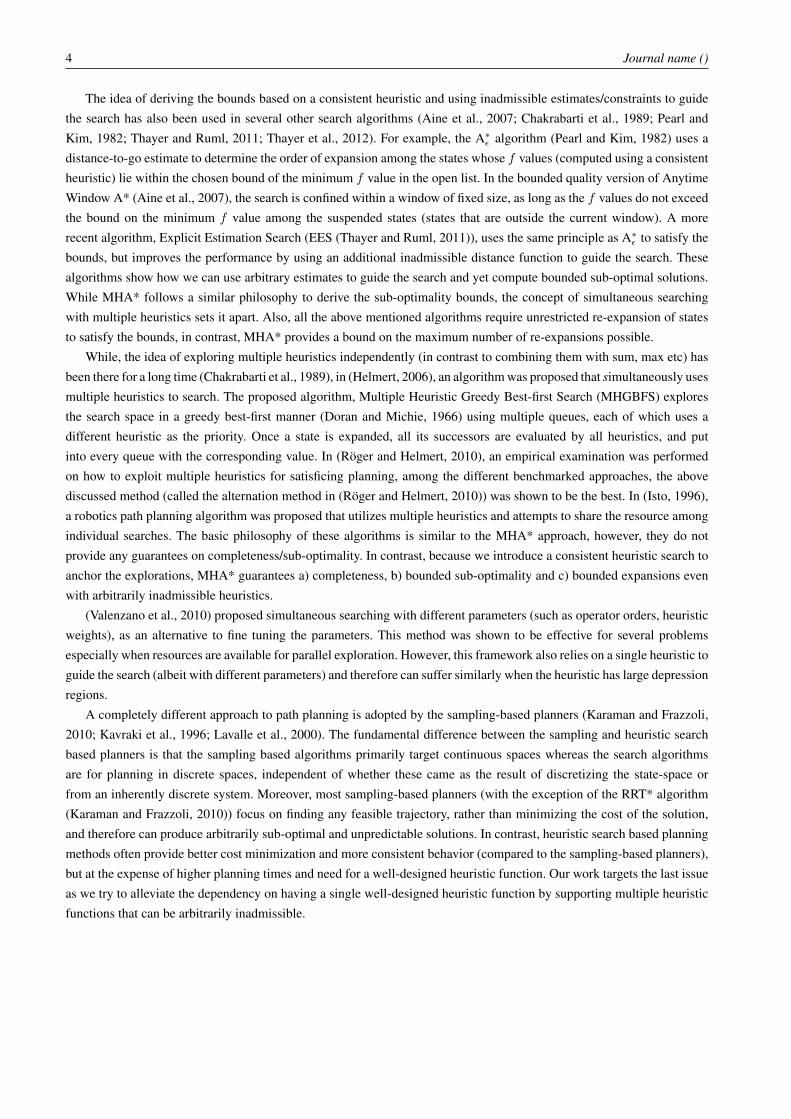
The idea of deriving the bounds based on a consistent heuristic and using inadmissible estimates/constraints to guidethe search has also been used in several other search algorithms (Aine et al., 2007; Chakrabarti et al., 1989; Pearl andKim, 1982; Thayer and Ruml, 2011; Thayer et al., 2012). For example, the A∗ε algorithm (Pearl and Kim, 1982) uses adistance-to-go estimate to determine the order of expansion among the states whose f values (computed using a consistentheuristic) lie within the chosen bound of the minimum f value in the open list. In the bounded quality version of AnytimeWindow A* (Aine et al., 2007), the search is confined within a window of fixed size, as long as the f values do not exceedthe bound on the minimum f value among the suspended states (states that are outside the current window). A morerecent algorithm, Explicit Estimation Search (EES (Thayer and Ruml, 2011)), uses the same principle as A∗ε to satisfy thebounds, but improves the performance by using an additional inadmissible distance function to guide the search. Thesealgorithms show how we can use arbitrary estimates to guide the search and yet compute bounded sub-optimal solutions.While MHA* follows a similar philosophy to derive the sub-optimality bounds, the concept of simultaneous searchingwith multiple heuristics sets it apart. Also, all the above mentioned algorithms require unrestricted re-expansion of statesto satisfy the bounds, in contrast, MHA* provides a bound on the maximum number of re-expansions possible.

While, the idea of exploring multiple heuristics independently (in contrast to combining them with sum, max etc) hasbeen there for a long time (Chakrabarti et al., 1989), in (Helmert, 2006), an algorithm was proposed that simultaneously usesmultiple heuristics to search. The proposed algorithm, Multiple Heuristic Greedy Best-first Search (MHGBFS) exploresthe search space in a greedy best-first manner (Doran and Michie, 1966) using multiple queues, each of which uses adifferent heuristic as the priority. Once a state is expanded, all its successors are evaluated by all heuristics, and putinto every queue with the corresponding value. In (Röger and Helmert, 2010), an empirical examination was performedon how to exploit multiple heuristics for satisficing planning, among the different benchmarked approaches, the abovediscussed method (called the alternation method in (Röger and Helmert, 2010)) was shown to be the best. In (Isto, 1996),a robotics path planning algorithm was proposed that utilizes multiple heuristics and attempts to share the resource amongindividual searches. The basic philosophy of these algorithms is similar to the MHA* approach, however, they do notprovide any guarantees on completeness/sub-optimality. In contrast, because we introduce a consistent heuristic search toanchor the explorations, MHA* guarantees a) completeness, b) bounded sub-optimality and c) bounded expansions evenwith arbitrarily inadmissible heuristics.

(Valenzano et al., 2010) proposed simultaneous searching with different parameters (such as operator orders, heuristicweights), as an alternative to fine tuning the parameters. This method was shown to be effective for several problemsespecially when resources are available for parallel exploration. However, this framework also relies on a single heuristic toguide the search (albeit with different parameters) and therefore can suffer similarly when the heuristic has large depressionregions.

A completely different approach to path planning is adopted by the sampling-based planners (Karaman and Frazzoli,2010; Kavraki et al., 1996; Lavalle et al., 2000). The fundamental difference between the sampling and heuristic searchbased planners is that the sampling based algorithms primarily target continuous spaces whereas the search algorithmsare for planning in discrete spaces, independent of whether these came as the result of discretizing the state-space orfrom an inherently discrete system. Moreover, most sampling-based planners (with the exception of the RRT* algorithm(Karaman and Frazzoli, 2010)) focus on finding any feasible trajectory, rather than minimizing the cost of the solution,and therefore can produce arbitrarily sub-optimal and unpredictable solutions. In contrast, heuristic search based planningmethods often provide better cost minimization and more consistent behavior (compared to the sampling-based planners),but at the expense of higher planning times and need for a well-designed heuristic function. Our work targets the last issueas we try to alleviate the dependency on having a single well-designed heuristic function by supporting multiple heuristicfunctions that can be arbitrarily inadmissible.

Multi-Heuristic A* 5

3. Multi-Heuristic A*

In this section, we describe two multi-heuristic search algorithms, IMHA* and SMHA*, and discuss their properties.Notations and Assumptions : In the following, S denotes the finite set of states of the domain. c(s, s′) denotes the

cost of the edge between s and s′, if there is no such edge, then c(s, s′) = ∞. We assume c(s, s′) ≥ 0, ∀s, s′ pairs.Succ(s) := {s′ ∈ S|c(s, s′) 6= ∞}, denotes the set of all successors of s. c∗(s, s′) denotes the cost of the optimal pathfrom state s to s′. g∗(s) denotes the optimal path cost from sstart to s. g(s) denotes the currently best known path costfrom sstart to s, and bp(s) denotes a back-pointer which points to the best predecessor of s (if computed).

We assume that we have n heuristics denoted by hi for i = 1, 2, . . . , n. These heuristics do not need to be consistent,in fact, they can be arbitrarily inadmissible. We also require access to a consistent (and thus admissible) heuristic (denotedby h0), i.e., h0 should satisfy, h0(sgoal) = 0 and h0(s) ≤ h0(s′) + c(s, s′), ∀s, s′ pair, where s′ ∈ Succ(s) and s 6= sgoal

(Pearl, 1984). MHA* uses separate priority queues for each search (n + 1 queues), denoted by OPENi, for i = 0..n.Throughout the rest of the paper, we will use the term anchor search to refer to the search that uses h0. Other searches willbe referred to as inadmissible searches. We assume that each priority queue (OPENi) supports a function OPENi.Minkey(),which returns the minimum key value among the states present in the priority queue if the queue is not empty, else it returns∞.

3.1. Independent Multi-Heuristic A* (IMHA*)

The algorithm IMHA* is presented in Algorithm 1. In IMHA*, different heuristics are explored independently by simul-taneously running n+ 1 searches, where each search uses its own priority queue. Therefore, in addition to the different hvalues, each state uses a different g (and bp) value for each search. We use g0 to denote the g for the anchor search, and gi(i = 1, 2, . . . , n) for the other searches.

The sub-optimality bound is controlled using two variables, namely, w1(≥ 1.0) which is used to inflate the heuristicvalues for each of the searches, and w2(≥ 1.0) which is used as a factor to prioritize the inadmissible searches over theanchor search. IMHA* runs the inadmissible searches in a round robin manner in a way which guarantees that the solutioncost will be within the sub-optimality bound w1 ∗ w2 of the optimal solution cost.

IMHA* starts with initializing search variables (lines 13-18) for all the searches. It then performs best-first expansionsin a round robin fashion from queues OPENi i = 1..n, as long as OPENi.Minkey() ≤ w2 ∗OPEN0.Minkey() (line 21). Ifthe check is violated for a given search, it is suspended and a state from OPEN0 is expanded in its place. This in turn canincrease OPEN0.Minkey() (lower bound) and thus re-activate the suspended search2.

Expansion of a state is done in a similar way as done in A*. Each state is expanded at most once for each search (line10) following the fact that WA* does not need to re-expand states to guarantee the sub-optimality bound (Likhachev et al.,2004). IMHA* terminates successfully, if any of the searches have OPENi.Minkey() value greater than or equal to the gvalue of sgoal (in that search) and g(sgoal) <∞, otherwise it terminates with no solution when OPEN0.Minkey() ≥ ∞.

Next, we discuss the theoretical properties of IMHA*. First, we note that the anchor search in IMHA* is a single shotWA* (without re-expansions) with a consistent heuristic function h0 (as used in (Likhachev et al., 2004; Richter et al.,2010)). Thus, all the results of such a WA* are equally applicable in the case of the anchor search in IMHA*. We startby presenting two key theorems for the anchor search which shall later be used to derive the properties of IMHA*. Atthis point, we introduce two assumptions that will be used for the proofs through out the paper. First, we assume that if

2 It should be noted that an expansion from OPEN0 can also decrease the lower bound and thus suspend more inadmissible searches. One admissibleway to get rid of this is to allow the lower bound to only increase, i.e., we store the initial value of OPEN0.Minkey() in a variable and later only updateit if OPEN0.Minkey() increases.

6 Journal name ()

Algorithm 1 Independent Multi-Heuristic A* (IMHA*)1: procedure Key(s, i)2: return gi(s) + w1 ∗ hi(s)3: procedure ExpandState(s, i)4: Remove s from OPENi5: for all s′ ∈ Succ(s) do6: if s′ was never generated in the ith search then7: gi(s

′) =∞; bpi(s′) = null

8: if gi(s′) > gi(s) + c(s, s′) then9: gi(s

′) = gi(s) + c(s, s′); bpi(s′) = s10: if s′ /∈ CLOSEDi then11: Insert/Update s′ in OPENi with Key(s′, i)

12: procedure Main()13: for i = 0, 1, . . . , n do14: OPENi ← ∅15: CLOSEDi ← ∅16: gi(sstart) = 0; gi(sgoal) =∞17: bpi(sstart) = bpi(sgoal) = null18: Insert sstart in OPENi with Key(sstart, i)

19: while OPEN0.Minkey() <∞ do20: for i = 1, 2, . . . , n do21: if OPENi.Minkey() ≤ w2 ∗ OPEN0.Minkey() then22: if gi(sgoal) ≤ OPENi.Minkey() then23: if gi(sgoal) <∞ then24: Terminate and return path pointed by bpi(sgoal)25: else26: s← OPENi.Top()27: ExpandState(s, i)28: Insert s in CLOSEDi29: else30: if g0(sgoal) ≤ OPEN0.Minkey() then31: if g0(sgoal) <∞ then32: terminate and return path pointed by bp0(sgoal)

33: else34: s← OPEN0.Top()35: ExpandState(s, 0)36: Insert s in CLOSED0

Multi-Heuristic A* 7

OPENi = ∅ (∀i = 0, 1, . . . , n), then its minimim key value is∞. We also assume that any state s with undefined gi andbpi values (s not generated in ith search) has gi(s) =∞ and bpi = null3.

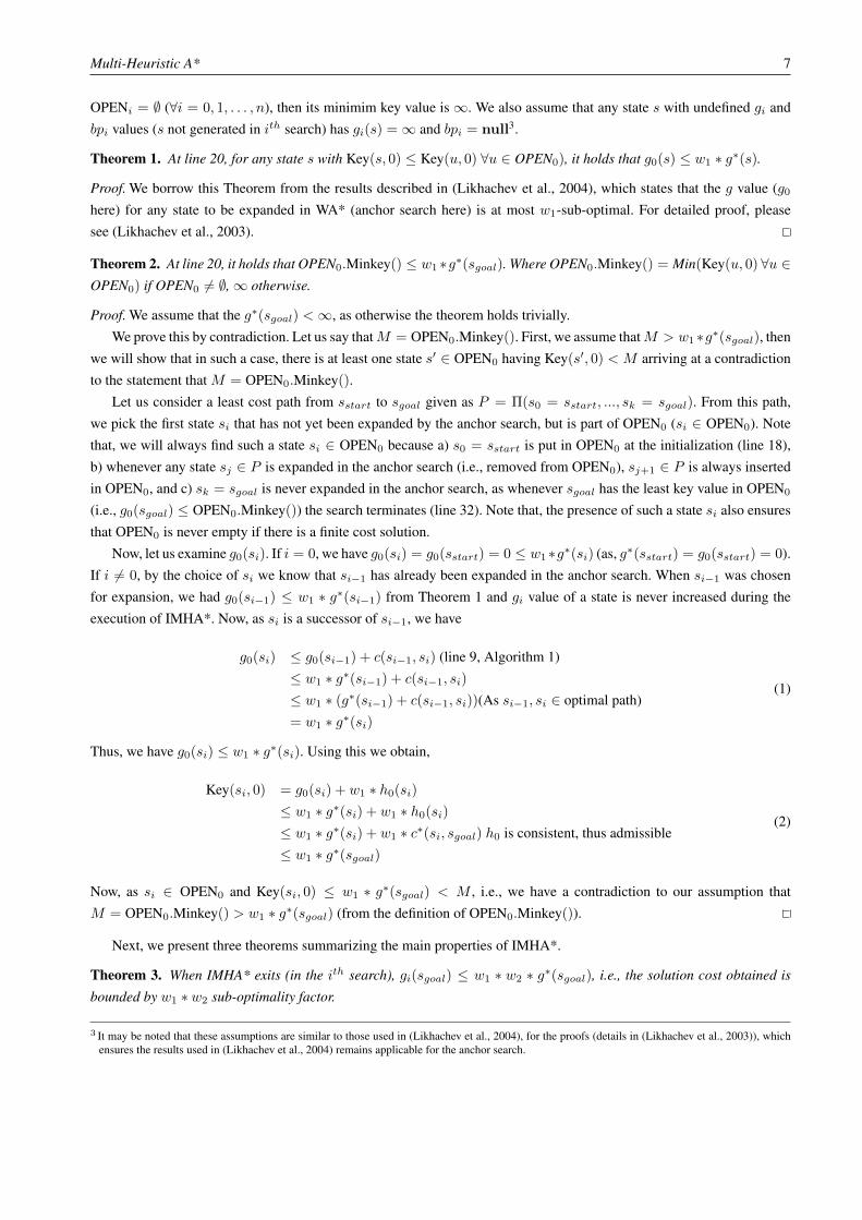
Theorem 1. At line 20, for any state s with Key(s, 0) ≤ Key(u, 0) ∀u ∈ OPEN0), it holds that g0(s) ≤ w1 ∗ g∗(s).

Proof. We borrow this Theorem from the results described in (Likhachev et al., 2004), which states that the g value (g0here) for any state to be expanded in WA* (anchor search here) is at most w1-sub-optimal. For detailed proof, pleasesee (Likhachev et al., 2003).

Theorem 2. At line 20, it holds that OPEN0.Minkey() ≤ w1 ∗g∗(sgoal). Where OPEN0.Minkey() = Min(Key(u, 0) ∀u ∈OPEN0) if OPEN0 6= ∅,∞ otherwise.

Proof. We assume that the g∗(sgoal) <∞, as otherwise the theorem holds trivially.We prove this by contradiction. Let us say thatM = OPEN0.Minkey(). First, we assume thatM > w1 ∗g∗(sgoal), then

we will show that in such a case, there is at least one state s′ ∈ OPEN0 having Key(s′, 0) < M arriving at a contradictionto the statement that M = OPEN0.Minkey().

Let us consider a least cost path from sstart to sgoal given as P = Π(s0 = sstart, ..., sk = sgoal). From this path,we pick the first state si that has not yet been expanded by the anchor search, but is part of OPEN0 (si ∈ OPEN0). Notethat, we will always find such a state si ∈ OPEN0 because a) s0 = sstart is put in OPEN0 at the initialization (line 18),b) whenever any state sj ∈ P is expanded in the anchor search (i.e., removed from OPEN0), sj+1 ∈ P is always insertedin OPEN0, and c) sk = sgoal is never expanded in the anchor search, as whenever sgoal has the least key value in OPEN0

(i.e., g0(sgoal) ≤ OPEN0.Minkey()) the search terminates (line 32). Note that, the presence of such a state si also ensuresthat OPEN0 is never empty if there is a finite cost solution.

Now, let us examine g0(si). If i = 0, we have g0(si) = g0(sstart) = 0 ≤ w1∗g∗(si) (as, g∗(sstart) = g0(sstart) = 0).If i 6= 0, by the choice of si we know that si−1 has already been expanded in the anchor search. When si−1 was chosenfor expansion, we had g0(si−1) ≤ w1 ∗ g∗(si−1) from Theorem 1 and gi value of a state is never increased during theexecution of IMHA*. Now, as si is a successor of si−1, we have

g0(si) ≤ g0(si−1) + c(si−1, si) (line 9, Algorithm 1)≤ w1 ∗ g∗(si−1) + c(si−1, si)

≤ w1 ∗ (g∗(si−1) + c(si−1, si))(As si−1, si ∈ optimal path)= w1 ∗ g∗(si)

(1)

Thus, we have g0(si) ≤ w1 ∗ g∗(si). Using this we obtain,

Key(si, 0) = g0(si) + w1 ∗ h0(si)

≤ w1 ∗ g∗(si) + w1 ∗ h0(si)

≤ w1 ∗ g∗(si) + w1 ∗ c∗(si, sgoal) h0 is consistent, thus admissible≤ w1 ∗ g∗(sgoal)

(2)

Now, as si ∈ OPEN0 and Key(si, 0) ≤ w1 ∗ g∗(sgoal) < M , i.e., we have a contradiction to our assumption thatM = OPEN0.Minkey() > w1 ∗ g∗(sgoal) (from the definition of OPEN0.Minkey()).

Next, we present three theorems summarizing the main properties of IMHA*.

Theorem 3. When IMHA* exits (in the ith search), gi(sgoal) ≤ w1 ∗ w2 ∗ g∗(sgoal), i.e., the solution cost obtained is

bounded by w1 ∗ w2 sub-optimality factor.

3 It may be noted that these assumptions are similar to those used in (Likhachev et al., 2004), for the proofs (details in (Likhachev et al., 2003)), whichensures the results used in (Likhachev et al., 2004) remains applicable for the anchor search.

8 Journal name ()

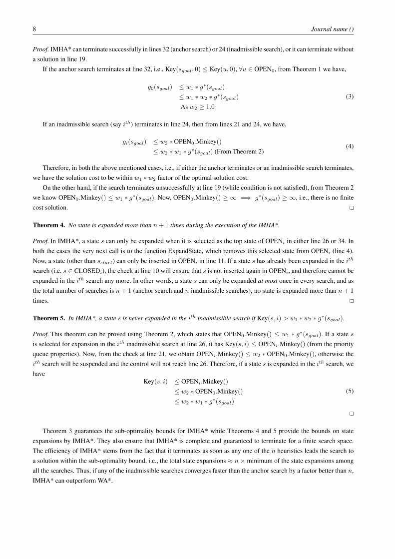
Proof. IMHA* can terminate successfully in lines 32 (anchor search) or 24 (inadmissible search), or it can terminate withouta solution in line 19.

If the anchor search terminates at line 32, i.e., Key(sgoal, 0) ≤ Key(u, 0), ∀u ∈ OPEN0, from Theorem 1 we have,

g0(sgoal) ≤ w1 ∗ g∗(sgoal)≤ w1 ∗ w2 ∗ g∗(sgoal)As w2 ≥ 1.0

(3)

If an inadmissible search (say ith) terminates in line 24, then from lines 21 and 24, we have,

gi(sgoal) ≤ w2 ∗ OPEN0.Minkey()

≤ w2 ∗ w1 ∗ g∗(sgoal) (From Theorem 2)(4)

Therefore, in both the above mentioned cases, i.e., if either the anchor terminates or an inadmissible search terminates,we have the solution cost to be within w1 ∗ w2 factor of the optimal solution cost.

On the other hand, if the search terminates unsuccessfully at line 19 (while condition is not satisfied), from Theorem 2we know OPEN0.Minkey() ≤ w1 ∗ g∗(sgoal). Now, OPEN0.Minkey() ≥ ∞ =⇒ g∗(sgoal) ≥ ∞, i.e., there is no finitecost solution.

Theorem 4. No state is expanded more than n+ 1 times during the execution of the IMHA*.

Proof. In IMHA*, a state s can only be expanded when it is selected as the top state of OPENi in either line 26 or 34. Inboth the cases the very next call is to the function ExpandState, which removes this selected state from OPENi (line 4).Now, a state (other than sstart) can only be inserted in OPENi in line 11. If a state s has already been expanded in the ith

search (i.e. s ∈ CLOSEDi), the check at line 10 will ensure that s is not inserted again in OPENi, and therefore cannot beexpanded in the ith search any more. In other words, a state s can only be expanded at most once in every search, and asthe total number of searches is n + 1 (anchor search and n inadmissible searches), no state is expanded more than n + 1

times.

Theorem 5. In IMHA*, a state s is never expanded in the ith inadmissible search if Key(s, i) > w1 ∗ w2 ∗ g∗(sgoal).

Proof. This theorem can be proved using Theorem 2, which states that OPEN0.Minkey() ≤ w1 ∗ g∗(sgoal). If a state sis selected for expansion in the ith inadmissible search at line 26, it has Key(s, i) ≤ OPENi.Minkey() (from the priorityqueue properties). Now, from the check at line 21, we obtain OPENi.Minkey() ≤ w2 ∗ OPEN0.Minkey(), otherwise theith search will be suspended and the control will not reach line 26. Therefore, if a state s is expanded in the ith search, wehave

Key(s, i) ≤ OPENi.Minkey()

≤ w2 ∗ OPEN0.Minkey()

≤ w2 ∗ w1 ∗ g∗(sgoal)(5)

Theorem 3 guarantees the sub-optimality bounds for IMHA* while Theorems 4 and 5 provide the bounds on stateexpansions by IMHA*. They also ensure that IMHA* is complete and guaranteed to terminate for a finite search space.The efficiency of IMHA* stems from the fact that it terminates as soon as any one of the n heuristics leads the search toa solution within the sub-optimality bound, i.e., the total state expansions ≈ n × minimum of the state expansions amongall the searches. Thus, if any of the inadmissible searches converges faster than the anchor search by a factor better than n,IMHA* can outperform WA*.

Multi-Heuristic A* 9

Algorithm 2 Shared Multi-Heuristic A* (SMHA*)1: procedure Key(s, i)2: return g(s) + w1 ∗ hi(s)3: procedure ExpandState(s)4: Remove s from OPENi ∀ i = 0, 1, . . . , n5: v(s) = g(s) . /* For proofs only. */6: for all s′ ∈ Succ(s) do7: if s′ was never generated then8: g(s′) =∞; bp(s′) = null9: v(s′) =∞ . /* For proofs only. */

10: if g(s′) > g(s) + c(s, s′) then11: g(s′) = g(s) + c(s, s′); bp(s′) = s12: if s′ /∈ CLOSEDanchor then13: Insert/Update s′ in OPEN0 with Key(s′, 0)14: if s′ /∈ CLOSEDinad then15: for i = 1, 2, . . . , n do16: if Key(s′, i) ≤ w2 ∗ Key(s′, 0) then17: Insert/Update s′ in OPENi with Key(s′, i)

18: procedure Main()19: g(sstart) = 0; g(sgoal) =∞20: bp(sstart) = bp(sgoal) = null21: v(sstart) = v(sgoal) =∞ . /* For proofs only. */22: for i = 0, 1, . . . , n do23: OPENi ← ∅24: Insert sstart in OPENi with Key(sstart, i)

25: CLOSEDanchor ← ∅26: CLOSEDinad ← ∅27: while OPEN0.Minkey() <∞ do28: for i = 1, 2, . . . , n do29: if OPENi.Minkey() ≤ w2 ∗ OPEN0.Minkey() then30: if g(sgoal) ≤ OPENi.Minkey() then31: if g(sgoal) <∞ then32: Terminate and return path pointed by bp(sgoal)33: else34: s← OPENi.Top()35: ExpandState(s)36: Insert s in CLOSEDinad37: else38: if g(sgoal) ≤ OPEN0.Minkey() then39: if g(sgoal) <∞ then40: terminate and return path pointed by bp(sgoal)41: else42: s← OPEN0.Top()43: ExpandState(s)44: Insert s in CLOSEDanchor

10 Journal name ()

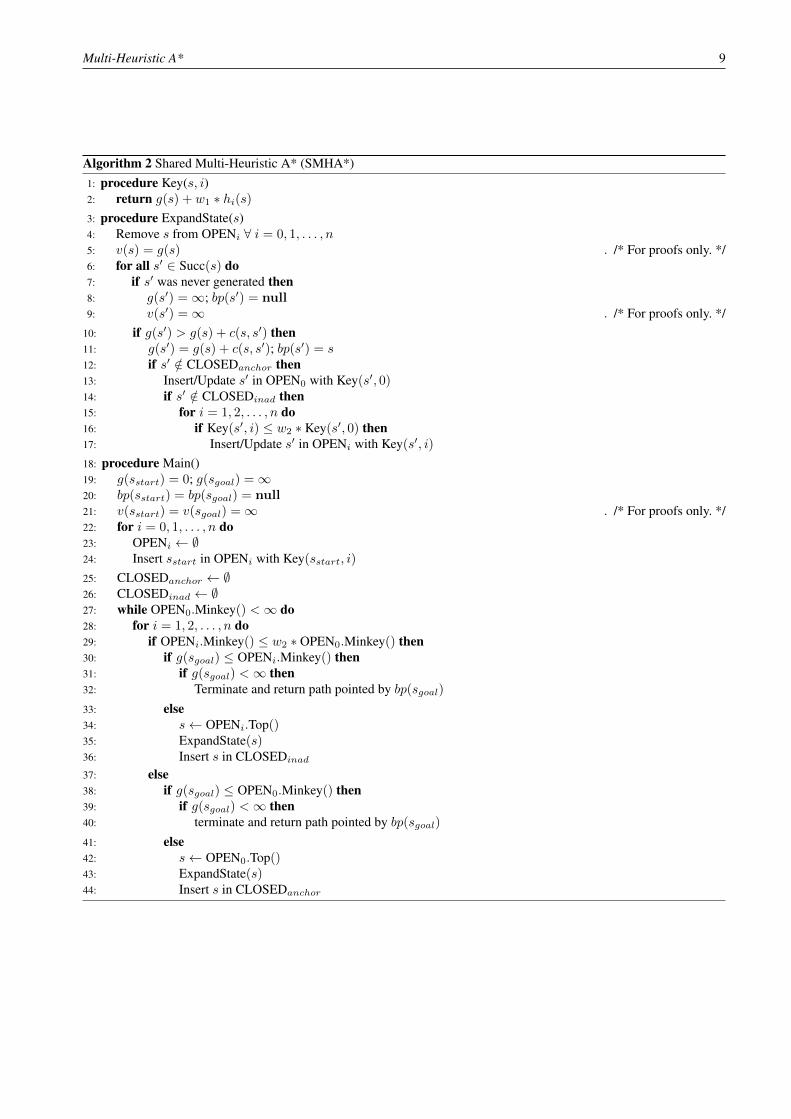
3.2. Shared Multi-Heuristic A* (SMHA*)

The primary difference between SMHA* and IMHA* is that in SMHA*, the current path for a given state is shared amongall the searches, i.e., if a better path to a state is discovered by any of the searches, the information is updated in all thepriority queues. As the paths are shared, SMHA* uses a single g (and bp) value for each state, unlike IMHA* in whichevery search maintains its own g value. Furthermore, path sharing allows SMHA* to expand each state at most twice, incontrast to IMHA* which may expand a state up to n+ 1 times (once in each search), and yet achieve the same bounds asIMHA*. We include the pseudocode for SMHA* in Algorithm 2. At this stage, the reader may ignore the mention of v(.)

in lines 5, 9 and 21 of the pseudocode presented (Algorithm 2), these lines are added for simplifying the proofs (discussedlater) and they do not impact the working of the algorithm.

The Key function and initialization part in SMHA* is the same as in IMHA* other than the fact that SMHA* usesa single g (and bp) variable. Also, IMHA* uses separate CLOSED lists for each search, in contrast SMHA* uses twoCLOSED lists, one for the anchor search (CLOSEDanchor) and another for all the inadmissible searches (CLOSEDinad).After the initialization, SMHA* runs the inadmissible searches in a round robin manner as long as the check in line 29 issatisfied. If the check is violated for a given search, it is suspended and a state is expanded from OPEN0.

The key difference between SMHA* and IMHA* lies in the state expansion method (ExpandState routine). In SMHA*,when a state s is expanded, its children (s′ ∈ Succ(s)) are simultaneously updated in all the priority queues, if s′ has notyet been expanded (lines 15-17). If s′ has been expanded in any of the inadmissible searches (s′ ∈ CLOSEDinad) but notin the anchor search (i.e., s′ /∈ CLOSEDanchor, check at line 12), it is inserted only in OPEN0. A state s′ that has beenexpanded in the anchor search (s′ ∈ CLOSEDanchor) is never re-expanded and thus, never put back into any of the priorityqueues.

The only exception to this simultaneous update (for a state s′ not yet expanded) is the optimization at line 16 whichensures that s′ is not put into OPENi if Key(s′, i) > w2 ∗ Key(s′, 0), because such a state will never be expanded fromOPENi anyway (check at line 29). The ExpandState routine also removes s from all OPENi (line 4) making sure that it isnever re-expanded again in any inadmissible search and not re-expanded in the anchor search if its g is not lowered.

If g(sgoal) becomes the minimum key value in any of the searches (anchor or inadmissible), SMHA* terminates with asolution within thew1∗w2 bound that can be obtained by greedily following the bp pointers from sgoal to sstart. Otherwise,no finite cost solution exists.

Next, we discuss the analytical properties of SMHA*. First, we should note that, unlike IMHA*, the anchor search inSMHA* is not a direct replica of a single shot WA* with a consistent heuristic function and, therefore, we cannot directlyuse the results for WA* (Theorem 1 and 2) to derive SMHA* properties. Instead, we follow a three step approach to provethe properties of SMHA*. We start by stating some low level properties, in the next phase we use these properties to obtainsome key results for the anchor search. Finally, we use those theorems to prove the correctness, bounded sub-optimalityand complexity results.

To simplify the proofs, we augment the pseudocode for SMHA* with lines 5, 9 and 21, which show that every state snow maintains an additional variable v(s), which is initially set to∞, and then is set to the g(s), when s is expanded in anyof the searches. It should be noted that this modification does not impact the working of SMHA* in any way as the v valuesare not used in the algorithm. We also extend the initialization assumption used for the IMHA* proofs to include v value,we assume that any state s with undefined v, g and bp values (i.e., s not generated by the search) has v(s) = g(s) = ∞and bp(s) = null.

Lemma 1. At any point of time during the execution of SMHA* and for any state s, we have v(s) ≥ g(s).

Proof. The lemma clearly holds before line 27 since at that point all the v values are infinite. Afterwards, g values can onlydecrease (line 11). For any state s, on the other hand, v(s) is initiated to∞ (line 9) and only changes on line 5 when it isset to g(s). Thus, it is always true that v(s) ≥ g(s).

Multi-Heuristic A* 11

Lemma 2. At line 27 (and line 28), all v and g values are non-negative, bp(sstart) = null, g(sstart) = 0 and for

∀s 6= sstart, bp(s) = argmin(s′∈Pred(s))v(s′) + c(s′, s), g(s) = v(bp(s)) + c(bp(s), s).

Proof. The lemma holds after the initialization, when g(sstart) = 0 while the rest of g values are∞, and all the v valuesare∞.

The only places where g and v values are changed afterwards are on lines 11 and 5. If v(s) is changed in line 5, then itis decreased according to Lemma 1. Thus, it may only decrease the g values of its successors. The test on line 10 checksthis and updates the g and bp values if necessary.

Since all costs are non-negative and they never change, g(sstart) can never be changed: it will never pass the test online 10, and thus is always 0. The Lemma thus holds.

Lemma 3. Suppose s is selected for expansion on lines 34 or 42. Then the next time line 28 is executed v(s) = g(s), where

g(s) before and after the expansion of s is the same.

Proof. Suppose s is selected for expansion. Then on line 5, v(s) = g(s), and it is the only place where a v value changes.We, thus, only need to show that g(s) does not change. It could only change if s ∈ Succ(s) and g(s) > v(s) + c(s, s).The second test, however, implies that c(s, s) < 0 since we have just set v(s) = g(s). This contradicts our assumption thatcosts are non-negative.

Next, we analyze the properties of the anchor search in SMHA* and show that it essentially follows the same lowerbound properties as IMHA* (Theorems 1 and 2). At an intuitive level, we can see that the lower bound results for SMHA*should be equivalent with IMHA*, as at any given point the OPEN0 in SMHA* can be viewed as a superset of OPEN0 inIMHA* (or WA* without re-expansions). This is due to the fact that whenever a state s is expanded in any of the searchesof SMHA* its children are put into OPEN0, thus it includes states from different searches. On the other hand, although s isdeleted from OPEN0 at this point (line 4), it can be re-inserted later if a better path to it is discovered (lowered g value), aslong as it has not yet been expanded in the anchor search. Now, as both Theorem 1 and 2 refer to the minimum key valuein OPEN0, the same bounds should hold for the anchor search in SMHA*.

However, to prove these results formally, we consider a set of states defined as follows,

Definition 1.Q = {u|v(u) > g(u)

∧v(u) > w1 ∗ g∗(u)} (6)

In other words, Q contains all the states that are generated but not yet expanded (v(u) 6= g(u)) and has v(u) more thanw1 times the best cost path between sstart and u.

Theorem 6. At line 27 (and line 28), let Q be defined according to the Definition 1. Then for any state s with Key(s, 0) ≤Key(u, 0) ∀u ∈ Q, it holds that g(s) ≤ w1 ∗ g∗(s).

Proof. We prove by contradiction.Suppose there exists an s such that Key(s, 0) ≤ Key(u, 0)∀u ∈ Q, but g(s) > w1 ∗ g∗(s). The latter implies that

g∗(s) <∞. We also assume that s 6= sstart since otherwise g(s) = 0 = g∗(s) (Lemma 2).Let us consider a least cost path from sstart to s given as P = Π(s0 = sstart, ..., sk = s). The cost of this path is

g∗(s). Such path must exist since g∗(s) <∞. Our assumption that g(s) > w1 ∗ g∗(s) means that there exists at least one

12 Journal name ()

si ∈ Π(s0, ..., sk−1) whose v(si) > w1 ∗ g∗(si). Otherwise,

g(s) = g(sk) ≤ v(sk−1) + c(sk−1, sk) (Lemma 2)≤ w1 ∗ g∗(sk−1) + c(sk−1, sk) (As v(si) ≤ w1 ∗ g∗(si) ∀si ∈ P )≤ w1 ∗ (g∗(sk−1) + c(sk−1, sk)) (As sk−1 ∈ optimal path to sk)≤ w1 ∗ g∗(sk) = w1 ∗ g∗(s)

(7)

Let us now consider si ∈ Π(s0, ..., sk−1) with the smallest index i ≥ 0 (that is, the closest to sstart ) such that v(si) >

w1 ∗ g∗(si). We will now show that si ∈ Q.If i = 0 then g(si) = g(sstart) = g∗(sstart) = 0 (Lemma 2). Thus, v(si) > w1 ∗ g∗(si) = 0 = g(si), and si ∈ Q. If

i > 0, we have v(si) > w1 ∗ g∗(si), and by the choice of si,

g(si) = min(s′∈Pred(si))v(s′) + c(s′, s)

≤ v(si−1) + c(si−1, si)

≤ w1 ∗ g∗(si−1) + c(si−1, si)

≤ w1 ∗ g∗(si)

(8)

We thus have v(si) > w1 ∗ g∗(si) ≥ g(si), which also implies that si ∈ Q.We will now show that Key(s, 0) > Key(si, 0), and finally arrive at a contradiction. According to our assumption,

Key(s, 0) = g(s) + w1 ∗ h0(s)

> w1 ∗ g∗(s) + w1 ∗ h0(s)

> w1 ∗ (g∗(si) + c∗(si, s) + h0(s))

> w1 ∗ g∗(si) + w1 ∗ h0(si) (h0 is consistent)> g(si) + w1 ∗ h0(si)

> Key(si, 0)

(9)

Now, as si ∈ Q and Key(si, 0) < Key(s, 0), we have a contradiction to our assumption that Key(s, 0) ≤ Key(u, 0),∀u ∈Q.

Theorem 7. At line 27 (as well as at line 28), let Q be defined according to the Definition 1. Then Q ⊆ OPEN0.

Proof. We prove this by induction. At the very start OPEN0 contains sstart, v(sstart) = ∞ and g(sstart) = 0, thus,sstart ∈ Q, obviously sstart ∈ OPEN0 (line 24). Also, for all other states s′, g(s′) = v(s′) =∞, thus the statement holds.

Now, we consider the states that are part of CLOSEDanchor. CLOSEDanchor holds all the states that are expanded in theanchor search at line 43 (insertion in line 44). Such a state s is removed from OPEN0 (and from all other OPENi, i 6= 0) atline 4 (before it is inserted in CLOSEDanchor). It follows that s ∈ CLOSEDanchor =⇒ s /∈ OPENi, ∀i, i = 0, 1, . . . , n,as a state s expanded in the anchor search will never be put back in any open list due to the check at line 12.

First, we show that the following statement, denoted by (*), holds for the first time line 27 is executed.(*): for any state s ∈ CLOSEDanchor, v(s) ≤ w1 ∗ g∗(s).This is obviously true as before the first execution of line 27, no state is expanded in the anchor search and thus

CLOSEDanchor is empty. We will now show by induction that the statement and the theorem continues to hold for theconsecutive executions of the line 27. Suppose the theorem and the statement (*) held during all the previous executionsof line 27. We need to show that the theorem holds the next time line 27 is executed.

We first prove that the statement (*) still holds during the next execution of line 27. Let us consider the for loop inline 28. From the induction hypothesis, we obtain that the theorem and the statement (*) is true before the first iteration ofthe for loop (as there are no other statements between line 27 and 28). We assume the theorem and statement (*) are true

Multi-Heuristic A* 13

for all for loop iterations prior to current iteration and show that they will remain true after the current iteration. Therefore,the statements will also remain true when the for loop ends and the control returns to line 27.

Considering the current iteration of the for loop, we observe the following possibilities, either the search terminates, inwhich case the theorem is proved trivially (as there will no more execution of line 27), or a state s is expanded either in aninadmissible search, i.e., from OPENi (i = 1, 2, . . . , n) or in the anchor search, i.e., from OPEN0.

Let us consider the first case, i.e., when s is selected for expansion in OPENi (line 34) and i 6= 0. This expansion (ofs) will only change v(s) (line 5) and no other state’s v will be altered. Also, as s is being expanded in an inadmissiblesearch, it follows that s /∈ CLOSEDanchor (as shown before) and thus there will be no change in the v-values of states thatare in CLOSEDanchor. Thus, all the states that are in CLOSEDanchor, satisfy v(s) ≤ w1 ∗ g∗(s) before and after such anexpansion (from the induction hypothesis). Thus, the statement (*) holds.

Now, consider the case when s is chosen for expansion in the anchor search (line 42). From the induction hypothesisQ ⊆ OPEN0, thus, selection of s guarantees g(s) ≤ w1 ∗ g∗(s) (Theorem 6). From Lemma 3, it also follows that nexttime line 28 is executed v(s) ≤ w1 ∗ g∗(s), and hence the statement (*) still holds as no other state’s v value has changedduring this expansion.

We now prove that after s is expanded (either in the anchor or in an inadmissible search) the theorem itself also holds.We assume that Q ⊆ OPEN0 held during all earlier iteration of the for loop and we prove it by showing that Q continuesto be a subset of OPEN0 after the current iteration. This will also prove that Q ⊆ OPEN0, when the next time line 27 isexecuted.

Any state that is generated for the first time in the ExpandState routine will be initialized with v(s) = g(s) =∞. Now,if during this expansion its g value is lowered then v(s) =∞ > g(s). Similarly, for all other states if the g value is lowered(at line 11), it would ensure v(s) > g(s), as either v(s) =∞ or v(s) holds the value g(s) when it was expanded last, nowthe g value has decreased (the g value of a state can only be altered at line 11, and this change can only lower the g valueas otherwise, the check at line 10 will never be true).

Each such state will be inserted/updated in OPEN0 at line 13, the only exception being if the check at line 12 is satisfied,i.e., s has earlier been expanded in the anchor search, in which case s ∈ CLOSEDanchor, and thus has v(s) ≤ w1 ∗ g∗(s),from statement (*).

All the states that have v(s) > g(s) are either ∈ OPEN0 or ∈ CLOSEDanchor. From statement (*) any state s ∈CLOSEDanchor satisfies v(s) ≤ w1 ∗ g∗(s). Therefore, for any state s, v(s) > g(s) and v(s) > w1 ∗ g∗(s), imply thats ∈ OPEN0. Which means, Q ⊆ OPEN0.

Thus proved.

Theorem 8. At line 28, for any state s with Key(s, 0) ≤ Key(u, 0) ∀u ∈ OPEN0, it holds that g(s) ≤ w1 ∗ g∗(s).

Proof. This theorem can be proved directly from the results of Theorem 6 and 7. From Theorem 7 we have Q ⊆ OPEN0,thus any state that satisfies Key(s, 0) ≤ Key(u, 0), ∀u ∈ OPEN0 also satisfies Key(s, 0) ≤ Key(u, 0) ∀u ∈ Q. Thus, fromTheorem 6, g(s) ≤ w1 ∗ g∗(s).

Theorem 9. At line 28, it holds that OPEN0.Minkey() ≤ w1 ∗ g∗(sgoal).

Proof. We can prove this in same manner as done for Theorem 2, utilizing Theorem 8 instead of Theorem 1.

Theorem 10. When SMHA* exits, g(sgoal) ≤ w1∗w2∗g∗(sgoal), i.e., the solution cost is bounded byw1∗w2 sub-optimality

factor.

Proof. This theorem can be proved in a manner similar to the proof for Theorem 3 using Theorems 8 and 9.

14 Journal name ()

Theorem 11. During the execution of SMHA*, a) no state is expanded more than twice, b) a state expanded in the anchor

search is never re-expanded, and c) a state expanded in an inadmissible search can only be re-expanded in the anchor

search if its g value is lowered.

Proof. In SMHA*, a state s can only be expanded when it is selected as the top state of OPENi in either line 34 or 42.If s is selected for expansion in line 34, the very next call is to the function ExpandState (line 35), which removes this

selected state from OPENi,∀i = 0..n (line 4). Also, after the ExpandState call, s is inserted in CLOSEDinad (line 36).Now, a state (other than sstart) can only be inserted in OPENi (i 6= 0) in line 17. If a state s has already been expandedin any of the inadmissible searches (i.e., s ∈ CLOSEDinad), the check at line 14 will ensure that s is not inserted again inOPENi (i 6= 0).Therefore, a state can only be expanded once in the inadmissible searches.

Now, when a state s is expanded in the anchor search, similar to the earlier case, here also, s is removed from all OPENi(line 4) and inserted to CLOSEDanchor. Thus, s can only be expanded again either in inadmissible searches or in anchorsearch, if it is re-inserted in any of the OPENi, which can only be done in lines 13 or 17. However, as s ∈ CLOSEDanchor,the check at line 12 will never be true, thus the control will never reach lines 13 or 17, i.e., s will never be re-expanded.Therefore, statement b) is true. Also, as s can be expanded at most once in the anchor search and at most once in theinadmissible searches, i.e., s cannot be expanded more than twice, proving statement a).

Finally, a state s that has been expanded in an inadmissible search, can only be expanded in the anchor search later ifit is re-inserted in OPEN0. A state can only be inserted in OPEN0 (any OPENi, for that matter) if the check at line 10 istrue, i.e., if its g value is less than its earlier g value. Thus, a state s whose g has not been lowered after its expansion in anyinadmissible search will never satisfy the condition at line 10 and will not be re-inserted in OPEN0 and thus, can never beexpanded in the anchor search. Therefore, statement c) is true.

Theorem 12. In SMHA*, a state s is never expanded in the ith inadmissible search if Key(s, i) > w1 ∗ w2 ∗ g∗(sgoal).

Proof. The proof is similar to Theorem 5, utilizing the fact that OPEN0.Minkey() ≤ w1 ∗ g∗(sgoal) (Theorem 9).

Theorem 10 shows that SMHA* guarantees the same sub-optimality bounds as IMHA* while Theorem 11 highlightsthe difference in complexity between these two approaches. In IMHA*, a state can be re-expanded at most n+ 1 times aseach search is performed independently, whereas in SMHA* the same bounds are attained with at most 1 re-expansion perstate (at most one expansion in inadmissible searches and one expansion the anchor search, when the state is first expandedin an inadmissible search and its g value is lowered). On the other hand, IMHA* has the following advantages over SMHA*,a) expansion of states in IMHA* is cheaper than SMHA* as SMHA* may require n + 1 insertion/update/removal steps,whereas IMHA* requires only 1, b) in SMHA* all the searches store a copy of each of the generated states, thus the memoryoverhead is more4, and c) IMHA* is more amenable to parallelization, as individual searches do not share information.

A more important distinction between SMHA* and IMHA* arises from the fact that as SMHA* shares the states and thebest path information among all the searches5, it can potentially use a combination of partial paths to exit from depressionregions, which is not possible in IMHA*. Therefore, if there are nested depression regions in the state space that none of theconsistent/inadmissible heuristics can avoid independently, SMHA* can outperform IMHA*. In Figure 2, we illustrate thisphenomenon with an example of a 12D planning problem. As shown in the figure, we use 3 heuristics here (1 consistent+ 2 inadmissible), however none of these heuristics can guide the search completely, as all of them get stuck in their ownlocal minimum. In such a scenario, SMHA* can use partial paths obtained by individual searches and seamlessly combinethem to obtain a complete plan (Figure 2f), but IMHA* cannot, as it does not share information. A video of the PR2 robotactually performing the task using the plan generated by SMHA* is included in Extension 1.

4 It may be noted that this memory overhead can be eliminated by using a single open list and making the update/insertion/removal more informed.5 SMHA* uses common g and bp values for all the searches. Also during each expansion, the children of the expanded state are inserted/updated in all

the priority queues making them available for selection according any of the heuristics.

Multi-Heuristic A* 15

(a) Problem instance (b) Consistent Heuristic (Base Distance) (c) Local Minimum: Base DistanceHeuristic

(d) Local Minimum: Goal OrientationHeuristic

(e) Local Minimum: Vertical OrientationHeuristic

(f) SMHA* Plan

Fig. 2. A full-body (12D) planning example highlighting the advantage of SMHA* over WA*/IMHA* for cases where no individualheuristic can escape all the depression regions by itself (nested depression regions). Here the task for the robot (PR2) is to carry a largeobject (picture frame) through a narrow corridor and a doorway, and then to put it down on a table. The problem instance is shown in2a with left and right figures depicting the start and end configurations, respectively. Figure 2b shows the vector field for a consistentheuristic (h0), computed by performing a backward (from goal to start) 2D search for the PR2 base. Figure 2c shows how a search usingh0 gets stuck (at the door) as it cannot orient the end-effector correctly, and thus ends up expanding a large number of states at the shownposition without moving toward the goal (deep local minimum) before running out of time (1 minute). To rectify this, we compute twoadditional (inadmissible) heuristics by including the orientation information for the end-effector, one targeting the goal orientation (h1)and another targeting a vertical orientation (h2). Unfortunately, none of these heuristics are powerful enough to take the search to thegoal state as they both suffer from their own depression regions (the searches using h1 and h2 gets stuck at different positions as shownin Figures 2d and 2e). As all the heuristics (consistent and inadmissible) lead the search to separate depression regions, IMHA* cannotavoid any of them and performs as poorly as WA*. However, as shown in Figure 2f, SMHA* can efficiently compute a plan by usingpartial paths from different heuristics. It uses the base and vertical orientation heuristic (in parts) go through the corridor and the door,and then switches to the goal orientation heuristic to align the end-effector to the goal.

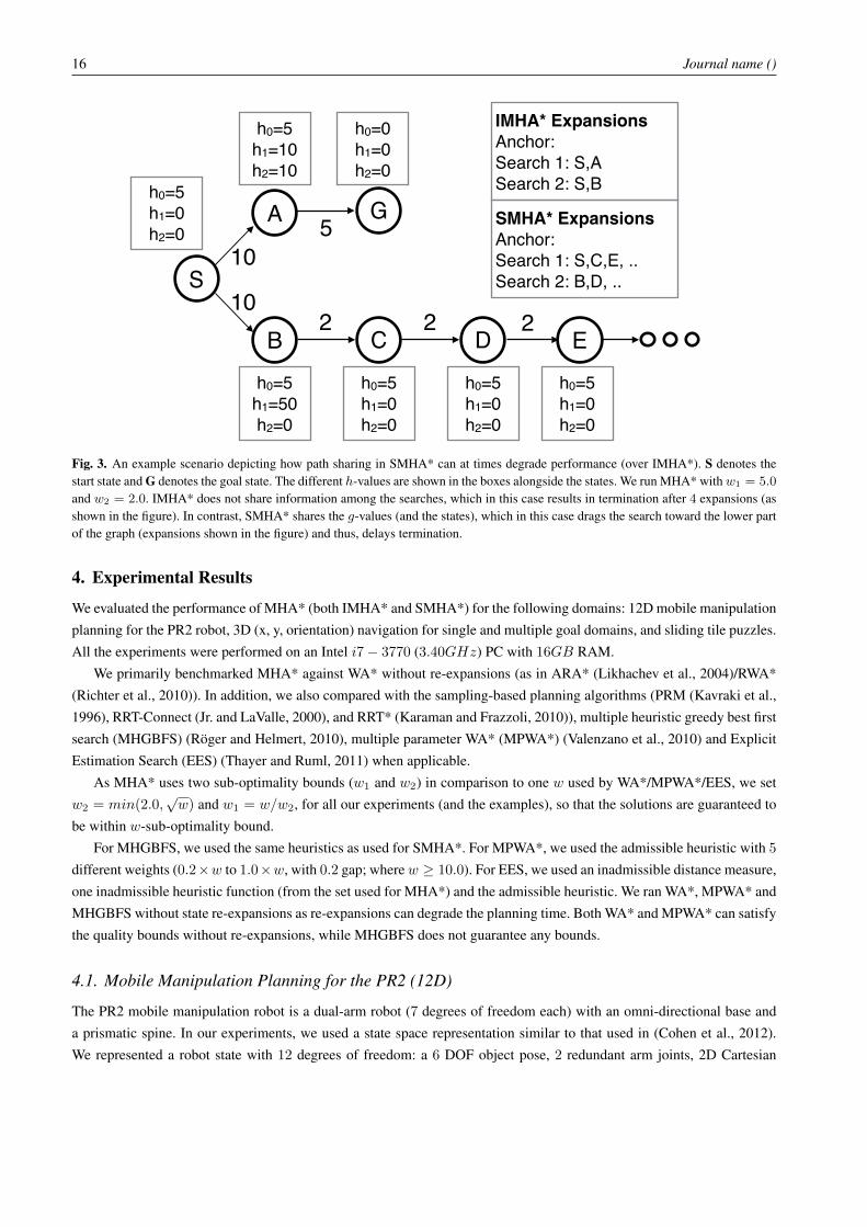
It should be noted that while sharing paths certainly makes SMHA* more powerful in handling nested minima, it canalso be counter-productive at times, especially if the path sharing drags the search to a local minimum that could have beenavoided if the searches were kept separate. Figure 3 includes an example of such a scenario with 3 heuristics (1 consistent +2 inadmissble). In this case, IMHA* terminates earlier than SMHA*, as path sharing leads both the inadmissible searchestoward the same local minimum.

16 Journal name ()

S

B

A

C D

Gh0=5h1=0h2=0

h0=5h1=10h2=10

h0=0h1=0h2=0

h0=5h1=50h2=0

h0=5h1=0h2=0

h0=5h1=0h2=0

10

10

5

2 2 2E

h0=5h1=0h2=0

IMHA* ExpansionsAnchor: Search 1: S,ASearch 2: S,B

SMHA* ExpansionsAnchor: Search 1: S,C,E, ..Search 2: B,D, ..

Fig. 3. An example scenario depicting how path sharing in SMHA* can at times degrade performance (over IMHA*). S denotes thestart state and G denotes the goal state. The different h-values are shown in the boxes alongside the states. We run MHA* with w1 = 5.0

and w2 = 2.0. IMHA* does not share information among the searches, which in this case results in termination after 4 expansions (asshown in the figure). In contrast, SMHA* shares the g-values (and the states), which in this case drags the search toward the lower partof the graph (expansions shown in the figure) and thus, delays termination.

4. Experimental Results

We evaluated the performance of MHA* (both IMHA* and SMHA*) for the following domains: 12D mobile manipulationplanning for the PR2 robot, 3D (x, y, orientation) navigation for single and multiple goal domains, and sliding tile puzzles.All the experiments were performed on an Intel i7− 3770 (3.40GHz) PC with 16GB RAM.

We primarily benchmarked MHA* against WA* without re-expansions (as in ARA* (Likhachev et al., 2004)/RWA*(Richter et al., 2010)). In addition, we also compared with the sampling-based planning algorithms (PRM (Kavraki et al.,1996), RRT-Connect (Jr. and LaValle, 2000), and RRT* (Karaman and Frazzoli, 2010)), multiple heuristic greedy best firstsearch (MHGBFS) (Röger and Helmert, 2010), multiple parameter WA* (MPWA*) (Valenzano et al., 2010) and ExplicitEstimation Search (EES) (Thayer and Ruml, 2011) when applicable.

As MHA* uses two sub-optimality bounds (w1 and w2) in comparison to one w used by WA*/MPWA*/EES, we setw2 = min(2.0,

√w) and w1 = w/w2, for all our experiments (and the examples), so that the solutions are guaranteed to

be within w-sub-optimality bound.For MHGBFS, we used the same heuristics as used for SMHA*. For MPWA*, we used the admissible heuristic with 5

different weights (0.2×w to 1.0×w, with 0.2 gap; wherew ≥ 10.0). For EES, we used an inadmissible distance measure,one inadmissible heuristic function (from the set used for MHA*) and the admissible heuristic. We ran WA*, MPWA* andMHGBFS without state re-expansions as re-expansions can degrade the planning time. Both WA* and MPWA* can satisfythe quality bounds without re-expansions, while MHGBFS does not guarantee any bounds.

4.1. Mobile Manipulation Planning for the PR2 (12D)

The PR2 mobile manipulation robot is a dual-arm robot (7 degrees of freedom each) with an omni-directional base anda prismatic spine. In our experiments, we used a state space representation similar to that used in (Cohen et al., 2012).We represented a robot state with 12 degrees of freedom: a 6 DOF object pose, 2 redundant arm joints, 2D Cartesian

Multi-Heuristic A* 17

coordinates for the base, an orientation of the base, and the prismatic spine height. The planner was provided the initialconfiguration of the robot as the start state. The goal state contained only the 6 DOF position of the object, which made itinherently under-specified because it provides no constraints on the position of the robot base or the redundant joint angles.The actions used to generate successors for states were a set of motion primitives, which are small, kinematically feasiblemotion sequences that move the object in 3D Cartesian space, rotate the redundant joint, or move the base in a typicallattice-type manner (Likhachev and Ferguson, 2009). The prismatic spine was also allowed to adjust its height in smallincrements.

We computed the admissible heuristic by taking the maximum value between the end-effector heuristic and the baseheuristic, where the end-effector heuristic was obtained by a 3D Dijkstra search initialized with the (x,y,z) coordinates ofthe goal and with all workspace obstacles inflated by their inner radius, and the base heuristic was obtained using a 2DDijkstra search for the robot base where the goal region is defined by a circular region centered around the (x,y) locationof the 6 DOF goal. The purpose of this circular region is to maintain an admissible heuristic despite having an incompletesearch goal. As the set of possible goal states must have the robot base within arm’s reach of the goal, we ensure that theheuristic always underestimates the actual cost to goal by setting the radius of the circular region to be slightly larger6

distance than the maximum reach of the robot arm.For IMHA*, we computed 2 additional heuristics in the following way. First, we randomly selected 2 points from the

base circle around the goal with valid inverse kinematic (IK) solutions for the arm to reach the goal and ran 2D Dijkstrabackward searches (to the start state) starting from these 2 points. This gave us two different base distances. Second, wecomputed an orientation distance by obtaining the angular difference between the current base orientation (at a given point)and the desired orientation, which was to make the robot face the end-effector goal. These distances (base and orientation)were then added to the end-effector heuristic to compute the final heuristic values. Note that this informative heuristic isclearly inadmissible, as they compute the angular and base distance difference for particular configurations, in contrast tofinding the minimum value among all possible configurations, but can still be used in the MHA* framework.

For SMHA*, we augmented this set by using the base (2D Dijkstra + orientation) and the end-effector heuristics (3DDijkstra) as two additional heuristics, since SMHA* can share the paths among the inadmissible searches, and hence, canpotentially benefit from not combining the two heuristics into a single one.

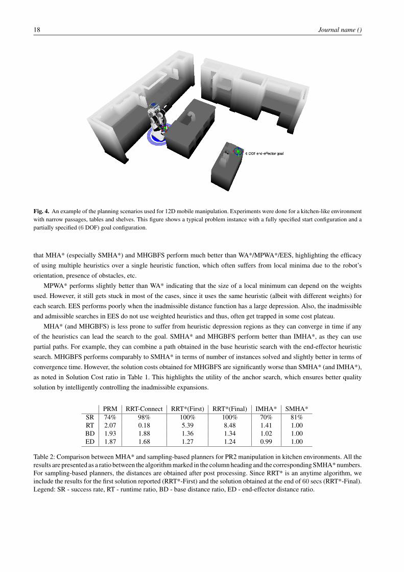
In Figure 4, we include an example of the test scenario with two large tables and a few narrow passageways. Foreach trial of the experiment, we randomly generated a full robot configuration anywhere in the kitchen for the start state,while generating a valid goal state that lies above the tabletops containing clutter. We generated 15 such environments byrandomly changing the object positions and for each such environment we used 10 different start and goal configurations.

WA* MHGBFS MPWA* EES IMHA* SMHA*SR 31% 76% 36% 27% 70% 81%SE 1.08 0.78 3.84 1.54 1.58 1.0RT 0.99 0.91 2.82 1.54 1.41 1.0SC 0.95 1.57 0.97 0.93 1.09 1.0

Table 1: Comparison between WA*, MHGBFS, MPWA*, EES and MHA* for PR2 manipulation planning in kitchenenvironments. The first row (SR) shows the percentage of total problem instances solved by each planner. The other rowsinclude the results as a ratio between the algorithm marked in the column heading and the corresponding SMHA* numbers,when both of them solved an instance. Legend: SR - success rate, SE - state expansion ratio, RT - runtime ratio, SC -solution cost ratio.

In Table 1, we include the results comparing WA*, EES, MPWA*, MHGBFS with the MHA*. We used w = 50

for all the algorithms. Each planner was given a maximum of 60 seconds to compute a plan. The results clearly show

6 We use a slightly larger distance to be conservative and thereby avoid any discretization errors which may make the heuristic inadmissible. However, ifperfect measurements are available, the exact value of the maximum reach of the robot arm can be used as the radius.

18 Journal name ()

Fig. 4. An example of the planning scenarios used for 12D mobile manipulation. Experiments were done for a kitchen-like environmentwith narrow passages, tables and shelves. This figure shows a typical problem instance with a fully specified start configuration and apartially specified (6 DOF) goal configuration.

that MHA* (especially SMHA*) and MHGBFS perform much better than WA*/MPWA*/EES, highlighting the efficacyof using multiple heuristics over a single heuristic function, which often suffers from local minima due to the robot’sorientation, presence of obstacles, etc.

MPWA* performs slightly better than WA* indicating that the size of a local minimum can depend on the weightsused. However, it still gets stuck in most of the cases, since it uses the same heuristic (albeit with different weights) foreach search. EES performs poorly when the inadmissible distance function has a large depression. Also, the inadmissibleand admissible searches in EES do not use weighted heuristics and thus, often get trapped in some cost plateau.

MHA* (and MHGBFS) is less prone to suffer from heuristic depression regions as they can converge in time if anyof the heuristics can lead the search to the goal. SMHA* and MHGBFS perform better than IMHA*, as they can usepartial paths. For example, they can combine a path obtained in the base heuristic search with the end-effector heuristicsearch. MHGBFS performs comparably to SMHA* in terms of number of instances solved and slightly better in terms ofconvergence time. However, the solution costs obtained for MHGBFS are significantly worse than SMHA* (and IMHA*),as noted in Solution Cost ratio in Table 1. This highlights the utility of the anchor search, which ensures better qualitysolution by intelligently controlling the inadmissible expansions.

PRM RRT-Connect RRT*(First) RRT*(Final) IMHA* SMHA*SR 74% 98% 100% 100% 70% 81%RT 2.07 0.18 5.39 8.48 1.41 1.00BD 1.93 1.88 1.36 1.34 1.02 1.00ED 1.87 1.68 1.27 1.24 0.99 1.00

Table 2: Comparison between MHA* and sampling-based planners for PR2 manipulation in kitchen environments. All theresults are presented as a ratio between the algorithm marked in the column heading and the corresponding SMHA* numbers.For sampling-based planners, the distances are obtained after post processing. Since RRT* is an anytime algorithm, weinclude the results for the first solution reported (RRT*-First) and the solution obtained at the end of 60 secs (RRT*-Final).Legend: SR - success rate, RT - runtime ratio, BD - base distance ratio, ED - end-effector distance ratio.

Multi-Heuristic A* 19

In Table 2, we include the results comparing MHA* with 3 sampling based algorithms, namely PRM, RRT-Connectand RRT*, in terms of runtime and solution quality. For the sampling-based algorithms we used the standard OMPL (Sucanet al., 2012) implementation. Since the sampling-based planners do not directly report the solution costs, in this table weinclude the results in terms of base and end-effector distances covered by the robots (after post processing). All the resultsare presented as a ratio over the corresponding SMHA* numbers for episodes where that planner and SMHA* were bothsuccessful in finding a solution within 60 seconds).

The results show that SMHA* performs reasonably well when compared to the sampling-based planners. Its runtimeis better than both PRM (5X) and RRT* (8X) but worse than RRT-Connect (5X). In terms of solution quality, MHA*results are noticeably better than all the sampling-based planners. However, both RRT-Connect and RRT* can solve morenumber of instances, mainly due to the facts that a) they are not bound by discretization choices and b) they do not useany heuristic function that may lead to local minima. Overall, the results show that MHA* (SMHA* in particular) is areasonable alternative for planning in such high-dimensional environments, especially when we are looking for predictable7

and bounded sub-optimal (with respect to the discretization choice) planning solutions.

4.2. 3D Path Planning (navigation)

While high dimensional problems like full-body planning for the PR2 are a true test-bed for assessing the real life applica-bility of MHA*, finding close-to-optimal solutions in such spaces is infeasible. Therefore, in order to get a better idea ofMHA*’s behavior for close-to-optimal bounds, we ran experiments in an easier 3D (x, y, orientation) navigation domain.

Here, we modeled our environment as a planar world and a rectangular polygonal robot with three degrees of freedom:x, y, and θ (heading). The search objective is to plan paths that satisfy the constraints on the minimum turning radius.The actions used to get successors for states are a set of motion primitives used in a lattice-type planner (Likhachev andFerguson, 2009). We computed the consistent heuristics (h0) by running a 16-connected 2D Dijkstra search assuming therobot is circular with a radius equal to the actual robot’s (PR2 base) inscribed circle, i.e., inflating the objects by the robot’sin-radius.

We used two kinds of environments for the testing: i) simulated indoor environments, which are composed of a seriesof randomly placed narrow hallways and large rooms with polygonal obstacles, and ii) simulated outdoor environments,which have relatively large open spaces with random regular shaped obstacles8, that occupy roughly 10−30% of the space.We generated 100 maps of 1000×1000 dimensions for both these environments. We performed the following experiments.

3D path planning with dual heuristics: In this experiment, in addition to h0, we generated an extra heuristic h1 byperforming another 2D Dijkstra search by inflating all the objects using the robot’s out-radius. Obviously, this heuristicfunction is an arbitrarily inadmissible one as a valid path can get blocked by such an inflation. On the other hand, h1 is lessprone to the local minima created due to minimum turning radius constraints.

In Figure 5, we include the results obtained for this experiment. The results show that for indoor environments, in termsof runtime, MHA* generally outperforms WA* by a significant margin. This is because, in indoor maps, the presence oflarge rooms and narrow corridors frequently creates big depression regions. MHA* can utilize the out-radius heuristic toquickly get away from such depression zones, while maintaining the quality bounds using the anchor search. In contrast,WA* only uses the in-radius heuristic guidance and thus often gets stuck in large local minima. For low sub-optimalitybounds, IMHA*’s performance degrades a bit compared to WA* due to re-expansions, however SMHA* still performsbetter. Overall, MHA* provides around 3X speed up over WA* while producing solutions of similar quality. In contrast,for outdoor environments, all the algorithms perform similarly for high bounds. In fact, in most cases, MHA* has a trifle

7 One of the issues with sampling based planners is that they often produce completely different solutions for problems that are very similar Phillips et al.(2012), in contrast, the search based planners tend to produce more predictable solutions.

8 We used circular, triangular and rectangular obstacles.

20 Journal name ()

weight IMHA* IMHA* SMHA* SMHA* IMHA* IMHA* SMHA* SMHA*

10 0.25 0.88 0.28 0.87 1.22 0.78 1.14 0.76

5 0.27 0.97 0.27 1 1.05 0.87 1.03 0.86

4 0.34 1.02 0.31 1.02 1.06 0.9 0.83 0.88

3 0.32 1 0.34 1 0.97 0.87 0.71 0.87

2 0.39 1.01 0.36 0.97 0.59 0.89 0.4 0.9

1.5 1.18 1.01 0.84 0.92 0.68 0.91 0.39 0.92

0.10

0.40

0.70

1.00

1.30

10 5 4 3 2 1.5

IMHA* SMHA*

0.80

0.90

1.00

1.10

1.20

10 5 4 3 2 1.5

IMHA* SMHA*

0.20

0.50

0.80

1.10

1.40

10 5 4 3 2 1.5

IMHA* SMHA*

0.70

0.80

0.90

1.00

1.10

10 5 4 3 2 1.5

IMHA* SMHA*

(a) Runtime ratio (indoor)

weight IMHA* IMHA* SMHA* SMHA* IMHA* IMHA* SMHA* SMHA*

10 0.25 0.88 0.28 0.87 1.22 0.78 1.14 0.76

5 0.27 0.97 0.27 1 1.05 0.87 1.03 0.86

4 0.34 1.02 0.31 1.02 1.06 0.9 0.83 0.88

3 0.32 1 0.34 1 0.97 0.87 0.71 0.87

2 0.39 1.01 0.36 0.97 0.59 0.89 0.4 0.9

1.5 1.18 1.01 0.84 0.92 0.68 0.91 0.39 0.92

0.10

0.40

0.70

1.00

1.30

10 5 4 3 2 1.5

IMHA* SMHA*

0.80

0.90

1.00

1.10

1.20

10 5 4 3 2 1.5

IMHA* SMHA*

0.20

0.50

0.80

1.10

1.40

10 5 4 3 2 1.5

IMHA* SMHA*

0.70

0.80

0.90

1.00

1.10

10 5 4 3 2 1.5

IMHA* SMHA*

(b) Solution cost ratio (indoor)

weight IMHA* IMHA* SMHA* SMHA* IMHA* IMHA* SMHA* SMHA*

10 0.25 0.88 0.28 0.87 1.22 0.78 1.14 0.76

5 0.27 0.97 0.27 1 1.05 0.87 1.03 0.86

4 0.34 1.02 0.31 1.02 1.06 0.9 0.83 0.88

3 0.32 1 0.34 1 0.97 0.87 0.71 0.87

2 0.39 1.01 0.36 0.97 0.59 0.89 0.4 0.9

1.5 1.18 1.01 0.84 0.92 0.68 0.91 0.39 0.92

0.10

0.40

0.70

1.00

1.30

10 5 4 3 2 1.5

IMHA* SMHA*

0.80

0.90

1.00

1.10

1.20

10 5 4 3 2 1.5

IMHA* SMHA*

0.20

0.50

0.80

1.10

1.40

10 5 4 3 2 1.5

IMHA* SMHA*

0.70

0.80

0.90

1.00

1.10

10 5 4 3 2 1.5

IMHA* SMHA*

(c) Runtime ratio (outdoor)

weight IMHA* IMHA* SMHA* SMHA* IMHA* IMHA* SMHA* SMHA*

10 0.25 0.88 0.28 0.87 1.22 0.78 1.14 0.76

5 0.27 0.97 0.27 1 1.05 0.87 1.03 0.86

4 0.34 1.02 0.31 1.02 1.06 0.9 0.83 0.88

3 0.32 1 0.34 1 0.97 0.87 0.71 0.87

2 0.39 1.01 0.36 0.97 0.59 0.89 0.4 0.9

1.5 1.18 1.01 0.84 0.92 0.68 0.91 0.39 0.92

0.10

0.40

0.70

1.00

1.30

10 5 4 3 2 1.5

IMHA* SMHA*

0.80

0.90

1.00

1.10

1.20

10 5 4 3 2 1.5

IMHA* SMHA*

0.20

0.50

0.80

1.10

1.40

10 5 4 3 2 1.5

IMHA* SMHA*

0.70

0.80

0.90

1.00

1.10

10 5 4 3 2 1.5

IMHA* SMHA*

(d) Solution cost ratio (outdoor)

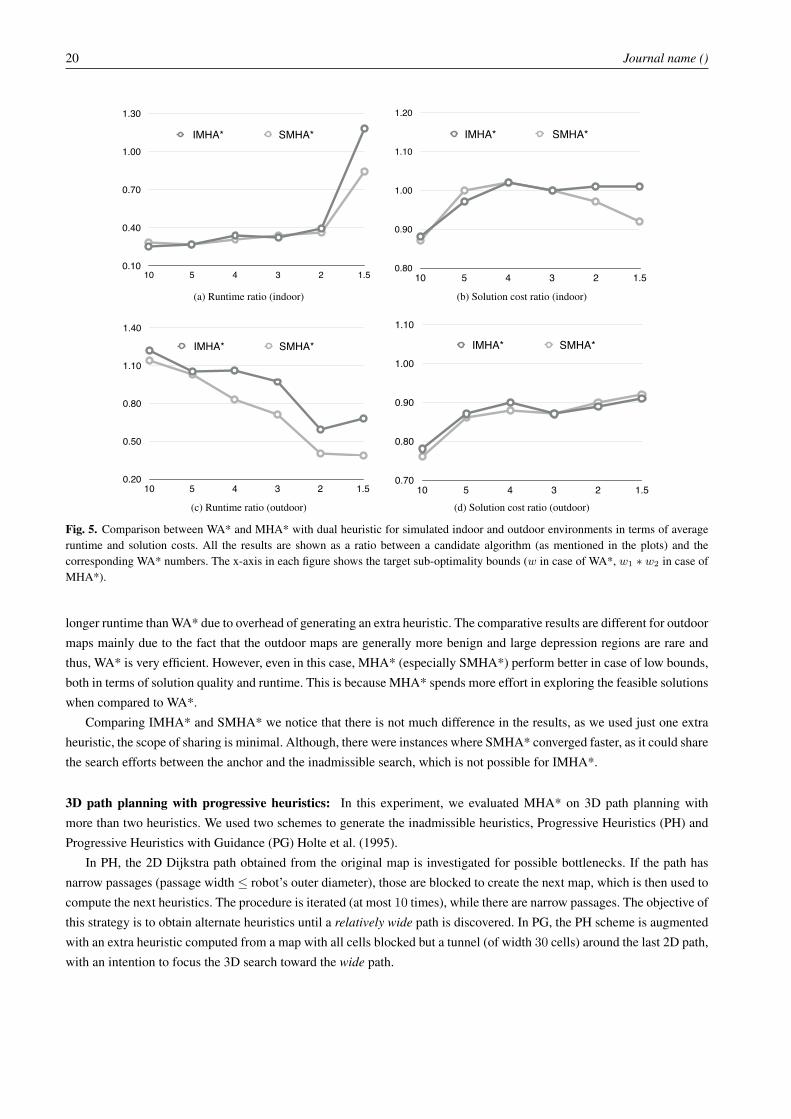
Fig. 5. Comparison between WA* and MHA* with dual heuristic for simulated indoor and outdoor environments in terms of averageruntime and solution costs. All the results are shown as a ratio between a candidate algorithm (as mentioned in the plots) and thecorresponding WA* numbers. The x-axis in each figure shows the target sub-optimality bounds (w in case of WA*, w1 ∗ w2 in case ofMHA*).

longer runtime than WA* due to overhead of generating an extra heuristic. The comparative results are different for outdoormaps mainly due to the fact that the outdoor maps are generally more benign and large depression regions are rare andthus, WA* is very efficient. However, even in this case, MHA* (especially SMHA*) perform better in case of low bounds,both in terms of solution quality and runtime. This is because MHA* spends more effort in exploring the feasible solutionswhen compared to WA*.

Comparing IMHA* and SMHA* we notice that there is not much difference in the results, as we used just one extraheuristic, the scope of sharing is minimal. Although, there were instances where SMHA* converged faster, as it could sharethe search efforts between the anchor and the inadmissible search, which is not possible for IMHA*.

3D path planning with progressive heuristics: In this experiment, we evaluated MHA* on 3D path planning withmore than two heuristics. We used two schemes to generate the inadmissible heuristics, Progressive Heuristics (PH) andProgressive Heuristics with Guidance (PG) Holte et al. (1995).

In PH, the 2D Dijkstra path obtained from the original map is investigated for possible bottlenecks. If the path hasnarrow passages (passage width ≤ robot’s outer diameter), those are blocked to create the next map, which is then used tocompute the next heuristics. The procedure is iterated (at most 10 times), while there are narrow passages. The objective ofthis strategy is to obtain alternate heuristics until a relatively wide path is discovered. In PG, the PH scheme is augmentedwith an extra heuristic computed from a map with all cells blocked but a tunnel (of width 30 cells) around the last 2D path,with an intention to focus the 3D search toward the wide path.

Multi-Heuristic A* 21

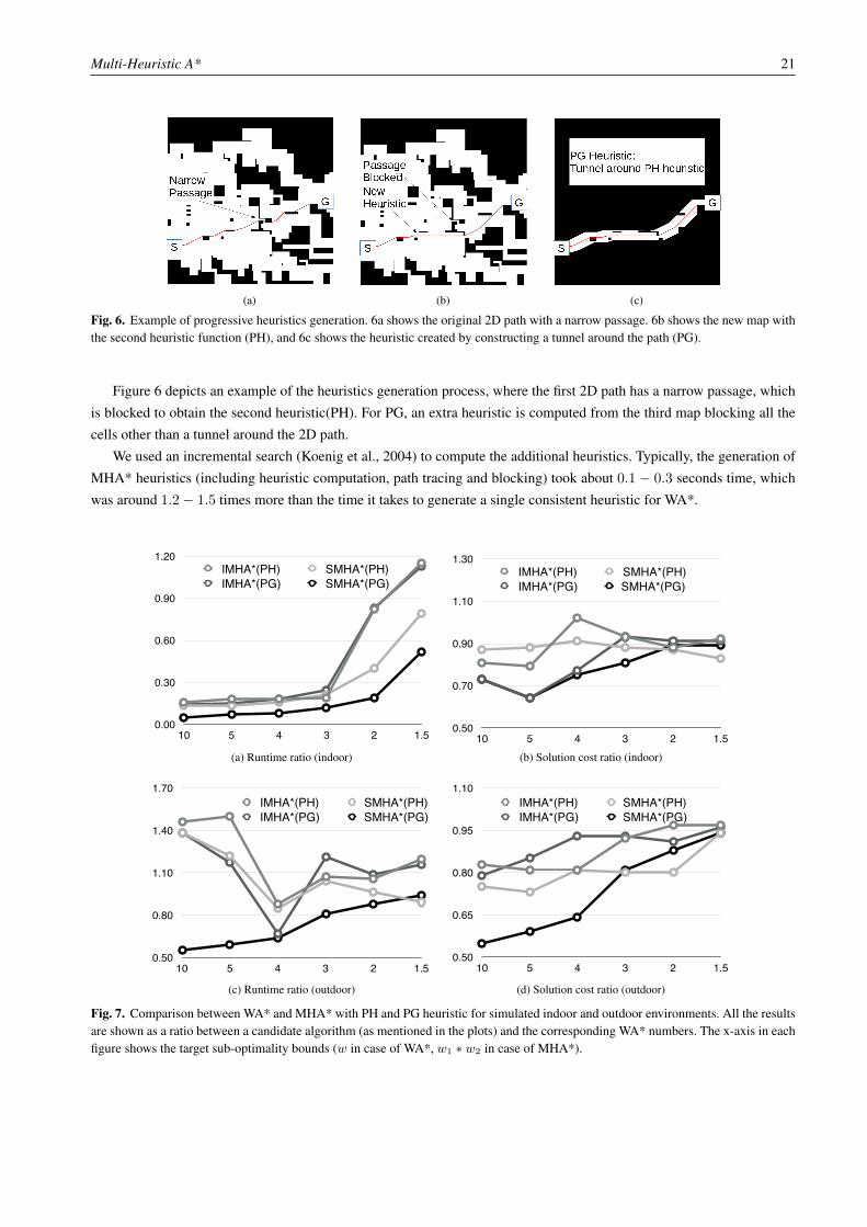
(a) (b) (c)

Fig. 6. Example of progressive heuristics generation. 6a shows the original 2D path with a narrow passage. 6b shows the new map withthe second heuristic function (PH), and 6c shows the heuristic created by constructing a tunnel around the path (PG).

Figure 6 depicts an example of the heuristics generation process, where the first 2D path has a narrow passage, whichis blocked to obtain the second heuristic(PH). For PG, an extra heuristic is computed from the third map blocking all thecells other than a tunnel around the 2D path.

We used an incremental search (Koenig et al., 2004) to compute the additional heuristics. Typically, the generation ofMHA* heuristics (including heuristic computation, path tracing and blocking) took about 0.1 − 0.3 seconds time, whichwas around 1.2− 1.5 times more than the time it takes to generate a single consistent heuristic for WA*.

W IMHA*(PH) IMHA*(PH) SMHA*(PH) SMHA*(PH) IMHA*(PG) IMHA*(PG) SMHA*(PG) SMHA*(PG) IMHA*(PH) IMHA*(PH) SMHA*(PH) SMHA*(PH) IMHA*(PG) IMHA*(PG) SMHA*(PG) SMHA*(PG)

10 0.16 0.81 0.13 0.87 0.14 0.73 0.05 0.73 1.46 0.83 1.38 0.75 1.38 0.79 1.38 0.55

5 0.18 0.79 0.13 0.88 0.15 0.64 0.07 0.64 1.5 0.81 1.22 0.73 1.17 0.85 1.06 0.59

4 0.18 1.02 0.16 0.91 0.18 0.77 0.08 0.75 0.88 0.81 0.85 0.81 0.67 0.93 0.67 0.64

3 0.19 0.93 0.21 0.88 0.24 0.93 0.12 0.81 1.07 0.92 1.04 0.8 1.21 0.93 0.82 0.81

2 0.82 0.88 0.4 0.87 0.83 0.91 0.19 0.89 1.06 0.97 0.96 0.8 1.09 0.91 0.74 0.88

1.5 1.15 0.92 0.79 0.83 1.13 0.91 0.52 0.89 1.2 0.97 0.89 0.94 1.16 0.96 0.87 0.94

0.00

0.30

0.60

0.90

1.20

10 5 4 3 2 1.5

IMHA*(PH) SMHA*(PH) IMHA*(PG) SMHA*(PG)

0.50

0.70

0.90

1.10

1.30

10 5 4 3 2 1.5

IMHA*(PH) SMHA*(PH) IMHA*(PG) SMHA*(PG)

0.50

0.80

1.10

1.40

1.70

10 5 4 3 2 1.5

IMHA*(PH) SMHA*(PH)IMHA*(PG) SMHA*(PG)

0.50

0.65

0.80

0.95

1.10

10 5 4 3 2 1.5

IMHA*(PH) SMHA*(PH)IMHA*(PG) SMHA*(PG)

(a) Runtime ratio (indoor)

W IMHA*(PH) IMHA*(PH) SMHA*(PH) SMHA*(PH) IMHA*(PG) IMHA*(PG) SMHA*(PG) SMHA*(PG) IMHA*(PH) IMHA*(PH) SMHA*(PH) SMHA*(PH) IMHA*(PG) IMHA*(PG) SMHA*(PG) SMHA*(PG)

10 0.16 0.81 0.13 0.87 0.14 0.73 0.05 0.73 1.46 0.83 1.38 0.75 1.38 0.79 1.38 0.55

5 0.18 0.79 0.13 0.88 0.15 0.64 0.07 0.64 1.5 0.81 1.22 0.73 1.17 0.85 1.06 0.59

4 0.18 1.02 0.16 0.91 0.18 0.77 0.08 0.75 0.88 0.81 0.85 0.81 0.67 0.93 0.67 0.64

3 0.19 0.93 0.21 0.88 0.24 0.93 0.12 0.81 1.07 0.92 1.04 0.8 1.21 0.93 0.82 0.81

2 0.82 0.88 0.4 0.87 0.83 0.91 0.19 0.89 1.06 0.97 0.96 0.8 1.09 0.91 0.74 0.88

1.5 1.15 0.92 0.79 0.83 1.13 0.91 0.52 0.89 1.2 0.97 0.89 0.94 1.16 0.96 0.87 0.94

0.00

0.30

0.60

0.90

1.20

10 5 4 3 2 1.5

IMHA*(PH) SMHA*(PH) IMHA*(PG) SMHA*(PG)

0.50

0.70

0.90

1.10

1.30

10 5 4 3 2 1.5

IMHA*(PH) SMHA*(PH) IMHA*(PG) SMHA*(PG)

0.50

0.80

1.10

1.40

1.70

10 5 4 3 2 1.5

IMHA*(PH) SMHA*(PH)IMHA*(PG) SMHA*(PG)

0.50

0.65

0.80

0.95

1.10

10 5 4 3 2 1.5

IMHA*(PH) SMHA*(PH)IMHA*(PG) SMHA*(PG)

(b) Solution cost ratio (indoor)

W IMHA*(PH) IMHA*(PH) SMHA*(PH) SMHA*(PH) IMHA*(PG) IMHA*(PG) SMHA*(PG) SMHA*(PG) IMHA*(PH) IMHA*(PH) SMHA*(PH) SMHA*(PH) IMHA*(PG) IMHA*(PG) SMHA*(PG) SMHA*(PG)

10 0.16 0.81 0.13 0.87 0.14 0.73 0.05 0.73 1.46 0.83 1.38 0.75 1.38 0.79 1.38 0.55

5 0.18 0.79 0.13 0.88 0.15 0.64 0.07 0.64 1.5 0.81 1.22 0.73 1.17 0.85 1.06 0.59

4 0.18 1.02 0.16 0.91 0.18 0.77 0.08 0.75 0.88 0.81 0.85 0.81 0.67 0.93 0.67 0.64

3 0.19 0.93 0.21 0.88 0.24 0.93 0.12 0.81 1.07 0.92 1.04 0.8 1.21 0.93 0.82 0.81

2 0.82 0.88 0.4 0.87 0.83 0.91 0.19 0.89 1.06 0.97 0.96 0.8 1.09 0.91 0.74 0.88

1.5 1.15 0.92 0.79 0.83 1.13 0.91 0.52 0.89 1.2 0.97 0.89 0.94 1.16 0.96 0.87 0.94

0.00

0.30

0.60

0.90

1.20

10 5 4 3 2 1.5

IMHA*(PH) SMHA*(PH) IMHA*(PG) SMHA*(PG)

0.50

0.70

0.90

1.10

1.30

10 5 4 3 2 1.5

IMHA*(PH) SMHA*(PH) IMHA*(PG) SMHA*(PG)

0.50

0.80

1.10

1.40

1.70

10 5 4 3 2 1.5

IMHA*(PH) SMHA*(PH)IMHA*(PG) SMHA*(PG)

0.50

0.65

0.80

0.95

1.10

10 5 4 3 2 1.5

IMHA*(PH) SMHA*(PH)IMHA*(PG) SMHA*(PG)

(c) Runtime ratio (outdoor)

W IMHA*(PH) IMHA*(PH) SMHA*(PH) SMHA*(PH) IMHA*(PG) IMHA*(PG) SMHA*(PG) SMHA*(PG) IMHA*(PH) IMHA*(PH) SMHA*(PH) SMHA*(PH) IMHA*(PG) IMHA*(PG) SMHA*(PG) SMHA*(PG)

10 0.16 0.81 0.13 0.87 0.14 0.73 0.05 0.73 1.46 0.83 1.38 0.75 1.38 0.79 1.38 0.55

5 0.18 0.79 0.13 0.88 0.15 0.64 0.07 0.64 1.5 0.81 1.22 0.73 1.17 0.85 1.06 0.59

4 0.18 1.02 0.16 0.91 0.18 0.77 0.08 0.75 0.88 0.81 0.85 0.81 0.67 0.93 0.67 0.64

3 0.19 0.93 0.21 0.88 0.24 0.93 0.12 0.81 1.07 0.92 1.04 0.8 1.21 0.93 0.82 0.81

2 0.82 0.88 0.4 0.87 0.83 0.91 0.19 0.89 1.06 0.97 0.96 0.8 1.09 0.91 0.74 0.88

1.5 1.15 0.92 0.79 0.83 1.13 0.91 0.52 0.89 1.2 0.97 0.89 0.94 1.16 0.96 0.87 0.94

0.00

0.30

0.60

0.90

1.20

10 5 4 3 2 1.5

IMHA*(PH) SMHA*(PH) IMHA*(PG) SMHA*(PG)

0.50

0.70

0.90

1.10

1.30

10 5 4 3 2 1.5

IMHA*(PH) SMHA*(PH) IMHA*(PG) SMHA*(PG)

0.50

0.80

1.10

1.40

1.70

10 5 4 3 2 1.5

IMHA*(PH) SMHA*(PH)IMHA*(PG) SMHA*(PG)

0.50

0.65

0.80

0.95

1.10

10 5 4 3 2 1.5

IMHA*(PH) SMHA*(PH)IMHA*(PG) SMHA*(PG)

(d) Solution cost ratio (outdoor)

Fig. 7. Comparison between WA* and MHA* with PH and PG heuristic for simulated indoor and outdoor environments. All the resultsare shown as a ratio between a candidate algorithm (as mentioned in the plots) and the corresponding WA* numbers. The x-axis in eachfigure shows the target sub-optimality bounds (w in case of WA*, w1 ∗ w2 in case of MHA*).

22 Journal name ()

We include the results for this experiment in Figure 7. While the overall trends resemble the observations with dualheuristics (i.e., MHA* provides considerable improvement of WA* for indoor cases), the difference between WA* andMHA* is even more pronounced with PH/PG schemes. For indoor environments, the PH scheme generated additionalheuristics for 44 maps (out of 100), whereas for outdoor environments, it generated additional heuristics for 8 maps only.On an average, for indoor environments, MHA* provides 18X-2X runtime improvement over single heuristic WA*. Runtimeresults for all the algorithms are similar in case of outdoor environments (at high bounds, MHA* is a bit worse). However,for low bound values (≤ 2.0), SMHA*(PG) outperforms WA* both in terms of runtime and solution quality. ComparingIMHA* and SMHA*, we observe that in this experiment SMHA* consistently outperforms IMHA*, highlighting theefficacy of path sharing to navigate around depression regions in a more robust manner. Also, for low bound values,IMHA* tends to re-expand a lot more states which considerably degrades its performance.

MHGBFS MPWA* IMHA* SMHA*IS 37 35 52 52RT 22.39 3.38 1.35 1.00SC 7.27 1.26 1.22 1.00

Table 3: Comparison between MHGBFS, MPWA*, and MHA* for 3D path planning. All the planners were given maximum5 secs to plan. IS denotes the number of instances solved. RT and SC denote the runtime and solution cost ratio over SMHA*.

In Table 3, we include the results comparing MHA* (PG) with the MHGBFS and MPWA* on the combined set of 52

hard instances (44 indoor + 8 outdoor), for which the PH scheme generated extra heuristics. For MHA* and MPWA*, weused w = 10.0. Each algorithm was given a maximum of 5 seconds to compute a plan. Overall, the comparison betweenMPWA* and MHA* show a similar trend as seen for the 12D planner. In contrast, MHGBFS’ performance degradesconsiderably for this domain as its greedy approach at times drives the search deeper into a local minimum. Unlike 12Dplanning, cost plateaus are rare here while large depression regions are pretty common, and thus, the greedy approach hurtsmore often than it helps.

4.3. Multiple Goal Path Planning

In this experiment, we investigate the multiple goal path planning problem for 3D (x, y, orientation) lattices. Here, theplanning objective is to plan a path to any of the goals from a given set. Such planning problems are common in real life,for example, if a parking lot has multiple open slots, an autonomous car needs to plan a path to any one of the availableslots, preferably the one closest to it. MHA* can be a good fit for such planning problems as it can simultaneously explorepaths to all the goals, using one (or more) heuristics targeted toward a particular goal.

We used two bounded sub-optimal search techniques to compare against MHA* for this domain. In the first technique(we call it Seq-A*), we sequentially searched for paths to individual goals, starting with the goal that has the minimumheuristic value (2D distance) and using the best cost in the previous searches as an upper bound constraint for the currentsearch, i.e., we prune the states that have f value (f = g + h) greater than or equal to the best solution obtained in theearlier iterations. In the second technique (Min-A*), we generated a single admissible heuristic for each state by usingthe minimum heuristic value across all goals (computed by running a single Dijkstra search considering all goals), andconducted WA* using this heuristic (with inflation).

We ran the MHA* algorithms in two modes, in the first case (MHA*-Ad), we used a consistent heuristic (as computedin Min-A*) for the anchor search and used individual (admissible) heuristics for the inadmissible searches. In the secondversion (MHA*-InAd) we used the same heuristic for the anchor but used outer-radius based inadmissible heuristics forthe other searches. We performed this experiment with indoor environments only (on 100 maps) by randomly selecting2− 4 goals.

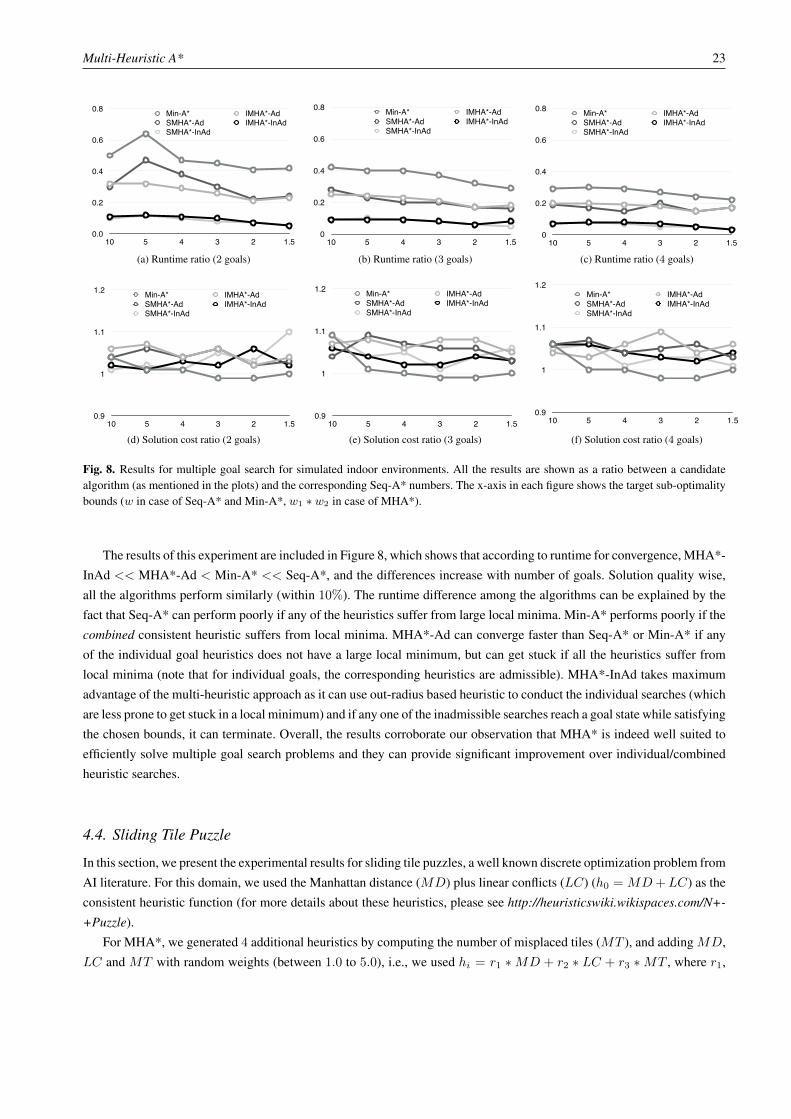
Multi-Heuristic A* 23

Goals W Min-A* Min-A* IMHA*-Ad IMHA*-Ad SMHA*-Ad SMHA*-Ad IMHA*-InAd IMHA*-InAd SMHA*-InAd SMHA*-InAd

0 10 0.5 1.04 0.32 1.06 0.3 1.04 0.11 1.02 0.1 1.01

0 5 0.64 1.01 0.32 1.07 0.47 1.06 0.12 1.01 0.12 1.02

2 4 0.47 1.01 0.29 1.04 0.38 1.04 0.11 1.03 0.1 1.01

0 3 0.45 0.99 0.26 1.06 0.3 1.06 0.1 1.02 0.08 1.05

0 2 0.41 0.99 0.21 1.02 0.22 1.02 0.07 1.06 0.07 1.03

0 1.5 0.42 1 0.23 1.04 0.24 1.03 0.05 1.02 0.05 1.1

Goals W Min-A* Min-A* IMHA*-Ad IMHA*-Ad SMHA*-Ad SMHA*-Ad IMHA*-InAd IMHA*-InAd SMHA*-InAd SMHA*-InAd

0 10 0.42 1.09 0.25 1.07 0.28 1.04 0.09 1.06 0.09 1.09

0 5 0.4 1.01 0.24 1.08 0.23 1.09 0.09 1.04 0.1 1.04

3 4 0.4 1 0.23 1.06 0.2 1.07 0.09 1.02 0.09 1.05

0 3 0.37 0.99 0.21 1.08 0.2 1.06 0.08 1.02 0.08 1.01

0 2 0.32 0.99 0.17 1.08 0.17 1.06 0.06 1.04 0.06 1.04

0 1.5 0.29 1 0.18 1.05 0.16 1.03 0.08 1.03 0.05 1.06

Goals W Min-A* Min-A* IMHA*-Ad IMHA*-Ad SMHA*-Ad SMHA*-Ad IMHA*-InAd IMHA*-InAd SMHA*-InAd SMHA*-InAd

0 10 0.29 1.06 0.2 1.04 0.19 1.06 0.07 1.06 0.07 1.05

0 5 0.3 1 0.2 1.03 0.17 1.07 0.08 1.06 0.08 1.06

4 4 0.29 1 0.19 1.06 0.15 1.04 0.08 1.04 0.07 1.01

0 3 0.27 0.98 0.18 1.09 0.2 1.05 0.07 1.03 0.05 1.03

0 2 0.24 0.98 0.15 1.04 0.15 1.06 0.05 1.02 0.05 1.03

0 1.5 0.22 1 0.17 1.06 0.17 1.03 0.03 1.04 0.03 1.01

0.0

0.2

0.4

0.6

0.8

10 5 4 3 2 1.5

Min-A* IMHA*-Ad SMHA*-Ad IMHA*-InAd SMHA*-InAd

0.9

1

1.1

1.2

10 5 4 3 2 1.5

Min-A* IMHA*-Ad SMHA*-Ad IMHA*-InAd SMHA*-InAd

(a) Runtime ratio (2 goals)

Goals W Min-A* Min-A* IMHA*-Ad IMHA*-Ad SMHA*-Ad SMHA*-Ad IMHA*-InAd IMHA*-InAd SMHA*-InAd SMHA*-InAd

0 10 0.42 1.09 0.25 1.07 0.28 1.04 0.09 1.06 0.09 1.09

0 5 0.4 1.01 0.24 1.08 0.23 1.09 0.09 1.04 0.1 1.04

3 4 0.4 1 0.23 1.06 0.2 1.07 0.09 1.02 0.09 1.05

0 3 0.37 0.99 0.21 1.08 0.2 1.06 0.08 1.02 0.08 1.01

0 2 0.32 0.99 0.17 1.08 0.17 1.06 0.06 1.04 0.06 1.04

0 1.5 0.29 1 0.18 1.05 0.16 1.03 0.08 1.03 0.05 1.06

Goals W Min-A* Min-A* IMHA*-Ad IMHA*-Ad SMHA*-Ad SMHA*-Ad IMHA*-InAd IMHA*-InAd SMHA*-InAd SMHA*-InAd

0 10 0.29 1.06 0.2 1.04 0.19 1.06 0.07 1.06 0.07 1.05

0 5 0.3 1 0.2 1.03 0.17 1.07 0.08 1.06 0.08 1.06

4 4 0.29 1 0.19 1.06 0.15 1.04 0.08 1.04 0.07 1.01

0 3 0.27 0.98 0.18 1.09 0.2 1.05 0.07 1.03 0.05 1.03

0 2 0.24 0.98 0.15 1.04 0.15 1.06 0.05 1.02 0.05 1.03

0 1.5 0.22 1 0.17 1.06 0.17 1.03 0.03 1.04 0.03 1.01

0

0.2

0.4

0.6

0.8

10 5 4 3 2 1.5

Min-A* IMHA*-Ad SMHA*-Ad IMHA*-InAd SMHA*-InAd

0.9

1

1.1

1.2

10 5 4 3 2 1.5

Min-A* IMHA*-Ad SMHA*-Ad IMHA*-InAd SMHA*-InAd

(b) Runtime ratio (3 goals)

Goals W Min-A* Min-A* IMHA*-Ad IMHA*-Ad SMHA*-Ad SMHA*-Ad IMHA*-InAd IMHA*-InAd SMHA*-InAd SMHA*-InAd

0 10 0.29 1.06 0.2 1.04 0.19 1.06 0.07 1.06 0.07 1.05

0 5 0.3 1 0.2 1.03 0.17 1.07 0.08 1.06 0.08 1.06

4 4 0.29 1 0.19 1.06 0.15 1.04 0.08 1.04 0.07 1.01

0 3 0.27 0.98 0.18 1.09 0.2 1.05 0.07 1.03 0.05 1.03

0 2 0.24 0.98 0.15 1.04 0.15 1.06 0.05 1.02 0.05 1.03

0 1.5 0.22 1 0.17 1.06 0.17 1.03 0.03 1.04 0.03 1.01

0

0.2

0.4

0.6

0.8

10 5 4 3 2 1.5

Min-A* IMHA*-Ad SMHA*-Ad IMHA*-InAd SMHA*-InAd

0.9

1

1.1

1.2

10 5 4 3 2 1.5

Min-A* IMHA*-Ad SMHA*-Ad IMHA*-InAd SMHA*-InAd

(c) Runtime ratio (4 goals)

Goals W Min-A* Min-A* IMHA*-Ad IMHA*-Ad SMHA*-Ad SMHA*-Ad IMHA*-InAd IMHA*-InAd SMHA*-InAd SMHA*-InAd

0 10 0.5 1.04 0.32 1.06 0.3 1.04 0.11 1.02 0.1 1.01

0 5 0.64 1.01 0.32 1.07 0.47 1.06 0.12 1.01 0.12 1.02

2 4 0.47 1.01 0.29 1.04 0.38 1.04 0.11 1.03 0.1 1.01

0 3 0.45 0.99 0.26 1.06 0.3 1.06 0.1 1.02 0.08 1.05

0 2 0.41 0.99 0.21 1.02 0.22 1.02 0.07 1.06 0.07 1.03

0 1.5 0.42 1 0.23 1.04 0.24 1.03 0.05 1.02 0.05 1.1

Goals W Min-A* Min-A* IMHA*-Ad IMHA*-Ad SMHA*-Ad SMHA*-Ad IMHA*-InAd IMHA*-InAd SMHA*-InAd SMHA*-InAd

0 10 0.42 1.09 0.25 1.07 0.28 1.04 0.09 1.06 0.09 1.09

0 5 0.4 1.01 0.24 1.08 0.23 1.09 0.09 1.04 0.1 1.04

3 4 0.4 1 0.23 1.06 0.2 1.07 0.09 1.02 0.09 1.05

0 3 0.37 0.99 0.21 1.08 0.2 1.06 0.08 1.02 0.08 1.01

0 2 0.32 0.99 0.17 1.08 0.17 1.06 0.06 1.04 0.06 1.04

0 1.5 0.29 1 0.18 1.05 0.16 1.03 0.08 1.03 0.05 1.06

Goals W Min-A* Min-A* IMHA*-Ad IMHA*-Ad SMHA*-Ad SMHA*-Ad IMHA*-InAd IMHA*-InAd SMHA*-InAd SMHA*-InAd

0 10 0.29 1.06 0.2 1.04 0.19 1.06 0.07 1.06 0.07 1.05

0 5 0.3 1 0.2 1.03 0.17 1.07 0.08 1.06 0.08 1.06

4 4 0.29 1 0.19 1.06 0.15 1.04 0.08 1.04 0.07 1.01

0 3 0.27 0.98 0.18 1.09 0.2 1.05 0.07 1.03 0.05 1.03

0 2 0.24 0.98 0.15 1.04 0.15 1.06 0.05 1.02 0.05 1.03

0 1.5 0.22 1 0.17 1.06 0.17 1.03 0.03 1.04 0.03 1.01

0.0

0.2

0.4

0.6

0.8

10 5 4 3 2 1.5

Min-A* IMHA*-Ad SMHA*-Ad IMHA*-InAd SMHA*-InAd

0.9

1

1.1

1.2

10 5 4 3 2 1.5

Min-A* IMHA*-Ad SMHA*-Ad IMHA*-InAd SMHA*-InAd

(d) Solution cost ratio (2 goals)

Goals W Min-A* Min-A* IMHA*-Ad IMHA*-Ad SMHA*-Ad SMHA*-Ad IMHA*-InAd IMHA*-InAd SMHA*-InAd SMHA*-InAd

0 10 0.42 1.09 0.25 1.07 0.28 1.04 0.09 1.06 0.09 1.09

0 5 0.4 1.01 0.24 1.08 0.23 1.09 0.09 1.04 0.1 1.04

3 4 0.4 1 0.23 1.06 0.2 1.07 0.09 1.02 0.09 1.05

0 3 0.37 0.99 0.21 1.08 0.2 1.06 0.08 1.02 0.08 1.01

0 2 0.32 0.99 0.17 1.08 0.17 1.06 0.06 1.04 0.06 1.04

0 1.5 0.29 1 0.18 1.05 0.16 1.03 0.08 1.03 0.05 1.06

Goals W Min-A* Min-A* IMHA*-Ad IMHA*-Ad SMHA*-Ad SMHA*-Ad IMHA*-InAd IMHA*-InAd SMHA*-InAd SMHA*-InAd

0 10 0.29 1.06 0.2 1.04 0.19 1.06 0.07 1.06 0.07 1.05

0 5 0.3 1 0.2 1.03 0.17 1.07 0.08 1.06 0.08 1.06

4 4 0.29 1 0.19 1.06 0.15 1.04 0.08 1.04 0.07 1.01

0 3 0.27 0.98 0.18 1.09 0.2 1.05 0.07 1.03 0.05 1.03

0 2 0.24 0.98 0.15 1.04 0.15 1.06 0.05 1.02 0.05 1.03

0 1.5 0.22 1 0.17 1.06 0.17 1.03 0.03 1.04 0.03 1.01

0

0.2

0.4

0.6

0.8

10 5 4 3 2 1.5

Min-A* IMHA*-Ad SMHA*-Ad IMHA*-InAd SMHA*-InAd

0.9

1

1.1

1.2

10 5 4 3 2 1.5

Min-A* IMHA*-Ad SMHA*-Ad IMHA*-InAd SMHA*-InAd

(e) Solution cost ratio (3 goals)

Goals W Min-A* Min-A* IMHA*-Ad IMHA*-Ad SMHA*-Ad SMHA*-Ad IMHA*-InAd IMHA*-InAd SMHA*-InAd SMHA*-InAd

0 10 0.29 1.06 0.2 1.04 0.19 1.06 0.07 1.06 0.07 1.05

0 5 0.3 1 0.2 1.03 0.17 1.07 0.08 1.06 0.08 1.06

4 4 0.29 1 0.19 1.06 0.15 1.04 0.08 1.04 0.07 1.01

0 3 0.27 0.98 0.18 1.09 0.2 1.05 0.07 1.03 0.05 1.03

0 2 0.24 0.98 0.15 1.04 0.15 1.06 0.05 1.02 0.05 1.03

0 1.5 0.22 1 0.17 1.06 0.17 1.03 0.03 1.04 0.03 1.01

0

0.2

0.4

0.6

0.8

10 5 4 3 2 1.5

Min-A* IMHA*-Ad SMHA*-Ad IMHA*-InAd SMHA*-InAd

0.9

1

1.1

1.2

10 5 4 3 2 1.5

Min-A* IMHA*-Ad SMHA*-Ad IMHA*-InAd SMHA*-InAd

(f) Solution cost ratio (4 goals)

Fig. 8. Results for multiple goal search for simulated indoor environments. All the results are shown as a ratio between a candidatealgorithm (as mentioned in the plots) and the corresponding Seq-A* numbers. The x-axis in each figure shows the target sub-optimalitybounds (w in case of Seq-A* and Min-A*, w1 ∗ w2 in case of MHA*).

The results of this experiment are included in Figure 8, which shows that according to runtime for convergence, MHA*-InAd << MHA*-Ad < Min-A* << Seq-A*, and the differences increase with number of goals. Solution quality wise,all the algorithms perform similarly (within 10%). The runtime difference among the algorithms can be explained by thefact that Seq-A* can perform poorly if any of the heuristics suffer from large local minima. Min-A* performs poorly if thecombined consistent heuristic suffers from local minima. MHA*-Ad can converge faster than Seq-A* or Min-A* if anyof the individual goal heuristics does not have a large local minimum, but can get stuck if all the heuristics suffer fromlocal minima (note that for individual goals, the corresponding heuristics are admissible). MHA*-InAd takes maximumadvantage of the multi-heuristic approach as it can use out-radius based heuristic to conduct the individual searches (whichare less prone to get stuck in a local minimum) and if any one of the inadmissible searches reach a goal state while satisfyingthe chosen bounds, it can terminate. Overall, the results corroborate our observation that MHA* is indeed well suited toefficiently solve multiple goal search problems and they can provide significant improvement over individual/combinedheuristic searches.

4.4. Sliding Tile Puzzle

In this section, we present the experimental results for sliding tile puzzles, a well known discrete optimization problem fromAI literature. For this domain, we used the Manhattan distance (MD) plus linear conflicts (LC) (h0 = MD+LC) as theconsistent heuristic function (for more details about these heuristics, please see http://heuristicswiki.wikispaces.com/N+-

+Puzzle).For MHA*, we generated 4 additional heuristics by computing the number of misplaced tiles (MT ), and adding MD,

LC and MT with random weights (between 1.0 to 5.0), i.e., we used hi = r1 ∗MD + r2 ∗ LC + r3 ∗MT , where r1,

24 Journal name ()

r2, r3 are random numbers between 1.0 and 5.0. Clearly, these heuristics are somewhat random and are inadmissible. Wetested the algorithms on 50 random instances (all solvable) of 48, 63 and 80 puzzles.

Time limit = 1 minute Time limit = 3 minutesSize Bound WA* IMHA* SMHA* WA*(R) WA* IMHA* SMHA* WA*(R)

50 46 49 50 49 47 49 50 5020 49 47 50 43 49 49 50 46

48 10 45 37 50 32 46 45 50 325 37 19 49 - 38 39 50 -2 12 4 9 - 12 6 10 -

50 25 35 40 26 29 38 44 3320 34 26 39 18 35 37 41 31

63 10 32 21 39 17 35 29 40 185 19 8 31 - 24 19 37 -2 3 4 4 - 7 4 9 -

50 17 24 31 15 22 26 33 2320 22 17 27 13 22 27 37 16

80 10 19 19 29 12 21 25 30 185 17 11 22 - 20 14 28 -2 7 1 4 - 7 1 9 -

Table 4: Number of sliding tile puzzle instances solved by WA*, IMHA* and SMHA* for different sub-optimality boundswith time limit 1 minute (columns 3, 4 and 5) and 3 minutes (columns 7, 8 and 9). WA*(R) columns (6 and 10) show theresults obtained by WA* used the same randomized heuristic, as used for MHA*.

In Table 4, we include the results in terms of the number of problems solved by all the algorithms under two timelimits: 1 minute and 3 minutes (we did not use larger time bounds due to memory limitations). The results show thateven with a randomized approach MHA*, especially SMHA*, can significantly outperform WA*. The performance gap ismore pronounced for larger sized problems and higher w values. For example, for 63 puzzle, SMHA* solved 44 instanceswhereas WA* could only solve 35 instances (IMHA* solved 38), for 80 puzzle, SMHA* solved 37 instances while WA*solved 22 instances only.

To highlight that the MHA* results were not due to the quality of randomized heuristic function, we include the results forWA* with a heuristic function (hr) generated using the same scheme as in MHA*, i.e., hr = r1∗MD+r2∗LC+r3∗MT ,where r1, r2, r3 are random numbers between 1.0 and 5.0 (referred to as WA*(R) in Table 4). As,hr ≤ 10∗h0, we computedthe results for sub-optimality bounds≥ 10 only. From Table 4, we see that the WA*(R) results are actually worse than WA*indicating that the improvements obtained by MHA* are due to their multi-heuristic exploration, which at times helped thesearch avoid getting trapped in depression regions.

In Table 5, we present the results obtained by comparing MHA* to MHGBFS and MPWA*. MHA*s and MPWA*were run with w = 20.0. All the algorithms were given a time limit of 1 minute. From the results, we observe that whileMPWA* and MHGBFS perform better in this domain (compared to path planning), overall, SMHA* still remains thebest algorithm. For each size, SMHA* could solve more or equal number (as in the case of 48 puzzle) of instances thanboth MPWA*/MHGBFS. Although MHGBFS had a better planning time in two scenarios, its solution quality is markedlyworse, as one would expect from the greedy approach.

Overall, the results from all these domains (from inherently continuous domains such as 12D motion planning to purelydiscrete domains such as sliding tile puzzles) highlight the potential of MHA* for solving complex optimization problemswhere it is hard to design a single consistent heuristic which effectively captures all the features of a given problem.Comparing two MHA* strategies, we observe that SMHA* generally dominates IMHA*, as it can combine the advantagesof three key MHA* principles, a) simultaneous exploration, b) sharing of partial paths, and c) controlling unnecessary

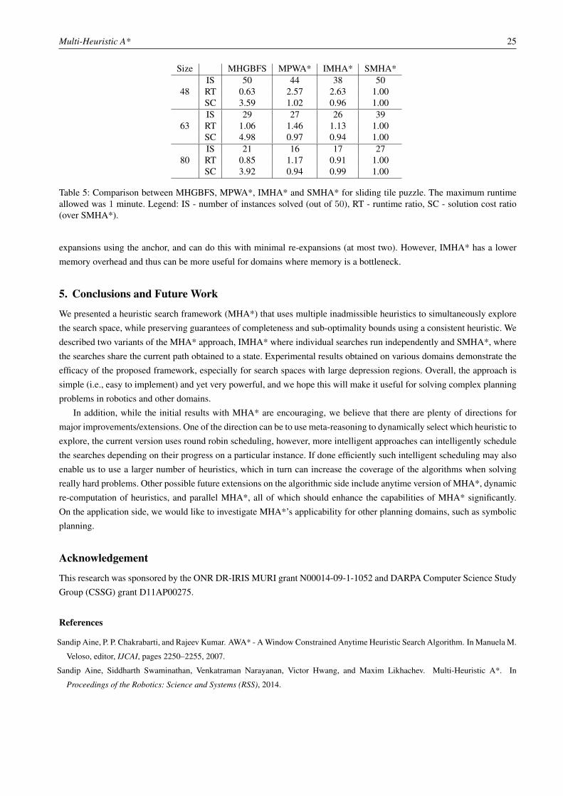
Multi-Heuristic A* 25

Size MHGBFS MPWA* IMHA* SMHA*IS 50 44 38 50

48 RT 0.63 2.57 2.63 1.00SC 3.59 1.02 0.96 1.00IS 29 27 26 39

63 RT 1.06 1.46 1.13 1.00SC 4.98 0.97 0.94 1.00IS 21 16 17 27

80 RT 0.85 1.17 0.91 1.00SC 3.92 0.94 0.99 1.00

Table 5: Comparison between MHGBFS, MPWA*, IMHA* and SMHA* for sliding tile puzzle. The maximum runtimeallowed was 1 minute. Legend: IS - number of instances solved (out of 50), RT - runtime ratio, SC - solution cost ratio(over SMHA*).

expansions using the anchor, and can do this with minimal re-expansions (at most two). However, IMHA* has a lowermemory overhead and thus can be more useful for domains where memory is a bottleneck.

5. Conclusions and Future Work

We presented a heuristic search framework (MHA*) that uses multiple inadmissible heuristics to simultaneously explorethe search space, while preserving guarantees of completeness and sub-optimality bounds using a consistent heuristic. Wedescribed two variants of the MHA* approach, IMHA* where individual searches run independently and SMHA*, wherethe searches share the current path obtained to a state. Experimental results obtained on various domains demonstrate theefficacy of the proposed framework, especially for search spaces with large depression regions. Overall, the approach issimple (i.e., easy to implement) and yet very powerful, and we hope this will make it useful for solving complex planningproblems in robotics and other domains.

In addition, while the initial results with MHA* are encouraging, we believe that there are plenty of directions formajor improvements/extensions. One of the direction can be to use meta-reasoning to dynamically select which heuristic toexplore, the current version uses round robin scheduling, however, more intelligent approaches can intelligently schedulethe searches depending on their progress on a particular instance. If done efficiently such intelligent scheduling may alsoenable us to use a larger number of heuristics, which in turn can increase the coverage of the algorithms when solvingreally hard problems. Other possible future extensions on the algorithmic side include anytime version of MHA*, dynamicre-computation of heuristics, and parallel MHA*, all of which should enhance the capabilities of MHA* significantly.On the application side, we would like to investigate MHA*’s applicability for other planning domains, such as symbolicplanning.

Acknowledgement

This research was sponsored by the ONR DR-IRIS MURI grant N00014-09-1-1052 and DARPA Computer Science StudyGroup (CSSG) grant D11AP00275.

References

Sandip Aine, P. P. Chakrabarti, and Rajeev Kumar. AWA* - A Window Constrained Anytime Heuristic Search Algorithm. In Manuela M.

Veloso, editor, IJCAI, pages 2250–2255, 2007.

Sandip Aine, Siddharth Swaminathan, Venkatraman Narayanan, Victor Hwang, and Maxim Likhachev. Multi-Heuristic A*. In

Proceedings of the Robotics: Science and Systems (RSS), 2014.

26 Journal name ()

Ronen I. Brafman, Hector Geffner, Jörg Hoffmann, and Henry A. Kautz, editors. Proceedings of the 20th International Conference on

Automated Planning and Scheduling, ICAPS 2010, Toronto, Ontario, Canada, May 12-16, 2010, 2010. AAAI.

P. P. Chakrabarti, Sujoy Ghose, A. Pandey, and S. C. De Sarkar. Increasing Search Efficiency Using Multiple Heuristics. Inf. Process.

Lett., 30(1):33–36, 1989.

P. P. Chakrabarti, Sujoy Ghose, and S. C. De Sarkar. Generalized best first search using single and multiple heuristics. Inf. Sci., 60(1-2):

145–175, 1992.

Benjamin Cohen, Sachin Chitta, and Maxim Likhachev. Single- and dual-arm motion planning with heuristic search. International

Journal of Robotics Research (IJRR), 2013.

Benjamin J. Cohen, Sachin Chitta, and Maxim Likhachev. Search-based planning for dual-arm manipulation with upright orientation

constraints. In ICRA, pages 3784–3790. IEEE, 2012. ISBN 978-1-4673-1403-9.

J. E. Doran and D. Michie. Experiments with the graph traverser program. In Brafman et al. (2010), pages 235–259.

A. Felner, R. E. Korf, and S. Hanan. Additive Pattern Database Heuristics. J. Artif. Intell. Res. (JAIR), 22:279–318, 2004.

P. E. Hart, N. J. Nilsson, and B. Raphael. A formal basis for the heuristic determination of minimum cost paths. IEEE Transactions on

Systems Science and Cybernetics, 4(2):100–107, July 1968.

Malte Helmert. The fast downward planning system. J. Artif. Intell. Res. (JAIR), 26:191–246, 2006.

C. Hernández and J. A. Baier. Avoiding and Escaping Depressions in Real-Time Heuristic Search. J. Artif. Intell. Res. (JAIR), 43:

523–570, 2012.

R.C. Holte, M.B. Perez, R.M. Zimmer, and A.J. MacDonald. The tradeoff between speed and optimality in hierarchical search. Technical

Report TR-95-19, School of Information Technology and Engineering. University of Ottawa. Canada, 1995.

Armin Hornung, Daniel Maier, and Maren Bennewitz. Search-based footstep planning. In Proc. of the ICRA Workshop on Progress and

Open Problems in Motion Planning and Navigation for Humanoids, Karlsruhe, Germany, May 2013.

Pekka Isto. Path planning by multiheuristic search via subgoals. In Proceedings of the 27th International Symposium on Industrial

Robots, CEU, pages 71272–6, 1996.

James J. Kuffner Jr. and Steven M. LaValle. RRT-Connect: An Efficient Approach to Single-Query Path Planning. In ICRA, pages

995–1001. IEEE, 2000. ISBN 0-7803-5889-9.

S. Karaman and E. Frazzoli. Incremental Sampling-based Algorithms for Optimal Motion Planning. In Robotics: Science and Systems,

Zaragoza, Spain, June 2010. The MIT Press.

Lydia E. Kavraki, Petr Svestka, Jean-Claude Latombe, and Mark H. Overmars. Probabilistic Roadmaps for Path Planning in High-

dimensional Configuration Spaces. IEEE T. Robotics and Automation, 12(4):566–580, 1996.

Sven Koenig, Maxim Likhachev, and David Furcy. Lifelong Planning A*. Artif. Intell., 155(1-2):93–146, 2004.

R. E. Korf and A. Felner. Disjoint pattern database heuristics. Artif. Intell., 134(1-2):9–22, 2002.

Steven M. Lavalle, James J. Kuffner, and Jr. Rapidly-exploring random trees: Progress and prospects. In Algorithmic and Computational

Robotics: New Directions, pages 293–308, 2000.

M. Likhachev, G. J. Gordon, and S. Thrun. Ara*: Formal analysis. Technical Report CMU-CS-03-148, School of Computer Science,

Carnegie Mellon University, Pittsburgh, PA 15213, 2003.

M. Likhachev, G. J. Gordon, and S. Thrun. ARA*: Anytime A* with Provable Bounds on Sub-Optimality. In Advances in Neural

Information Processing Systems 16. MIT Press, Cambridge, MA, 2004.

Maxim Likhachev and Dave Ferguson. Planning Long Dynamically Feasible Maneuvers for Autonomous Vehicles. I. J. Robotic Res.,

28(8):933–945, 2009.

Brian MacAllister, Jonathan Butzke, Aleksandr Kushleyev, and Maxim Likhachev. Path Planning for Non-Circular Micro Aerial Vehicles

in Constrained Environments. In Proceedings of the IEEE International Conference on Robotics and Automation (ICRA), pages

3933–3940, 2013.

Judea Pearl. Heuristics: intelligent search strategies for computer problem solving. Addison-Wesley Longman Publishing Co., Inc.,

Boston, MA, USA, 1984. ISBN 0-201-05594-5.

Multi-Heuristic A* 27

Judea Pearl and Jin H. Kim. Studies in Semi-Admissible Heuristics. IEEE Trans. Pattern Anal. Mach. Intell., 4(4):392–399, 1982.

Mike Phillips, Benjamin J. Cohen, Sachin Chitta, and Maxim Likhachev. E-graphs: Bootstrapping planning with experience graphs. In

Robotics: Science and Systems, 2012.

I. Pohl. Heuristic Search Viewed as Path Finding in a Graph. Artif. Intell., 1(3):193–204, 1970.

Silvia Richter, Jordan Tyler Thayer, and Wheeler Ruml. The Joy of Forgetting: Faster Anytime Search via Restarting. In Brafman et al.

(2010), pages 137–144.

Gabriele Röger and Malte Helmert. The More, the Merrier: Combining Heuristic Estimators for Satisficing Planning. In Brafman et al.

(2010), pages 246–249.

Ioan A. Sucan, Mark Moll, and Lydia E. Kavraki. The Open Motion Planning Library. IEEE Robotics & Automation Magazine, 19(4):

72–82, December 2012.

Jordan Tyler Thayer and Wheeler Ruml. Bounded Suboptimal Search: A Direct Approach Using Inadmissible Estimates. In IJCAI, pages

674–679, 2011.

Jordan Tyler Thayer, Roni Stern, Ariel Felner, and Wheeler Ruml. Faster Bounded-Cost Search Using Inadmissible Estimates. In Lee

McCluskey, Brian Williams, José Reinaldo Silva, and Blai Bonet, editors, ICAPS. AAAI, 2012. ISBN 978-1-57735-562-5.

Richard Anthony Valenzano, Nathan R. Sturtevant, Jonathan Schaeffer, Karen Buro, and Akihiro Kishimoto. Simultaneously Searching

with Multiple Settings: An Alternative to Parameter Tuning for Suboptimal Single-Agent Search Algorithms. In Brafman et al. (2010),

pages 177–184.

Chris. M. Wilt and Wheeler Ruml. When Does Weighted A* Fail? In SOCS. AAAI Press, 2012.

R. Zhou and E. A. Hansen. Multiple Sequence Alignment Using Anytime A*. In Proceedings of 18th National Conference on Artificial

Intelligence AAAI’2002, pages 975–976, 2002.

Matt Zucker, Nathan Ratliff, Martin Stole, Joel Chestnutt, J. Andrew Bagnell, Christopher G. Atkeson, and James Kuffner. Optimization

and learning for rough terrain legged locomotion. International Journal of Robotics Research, 30(2):175–191, 2011.