Embed Size (px)
Citation preview

10
Multi-level Models, and Repeated Measures
This chapter further extends the discussion of models that are a marked departure from theindependent errors models of Chapters 5 to 8. In the models that will be discussed in thischapter, there is a hierarchy of variation that corresponds to groupings within the data. Thegroups are nested. For example, students might be sampled from di↵erent classes, that inturn are sampled from di↵erent schools. Or, crop yields might be measured on multipleparcels of land at each of a number of di↵erent sites.
After fitting such models, predictions can be made at any of the di↵erent levels. Forexample crop yield could be predicted at new sites, or new parcels. Prediction for a newparcel at one of the existing sites is likely to be more accurate than a prediction for a totallynew site. Multi-level models, i.e. models which have multiple error (or noise) terms, areable to account for such di↵erences in predictive accuracy.
Repeated measures models are multi-level models where measurements consist of mul-tiple profiles in time or space; each profile can be viewed as a time series. Such data mayarise in a clinical trial, and animal or plant growth curves are common examples; each“individual” is measured at several di↵erent times. Typically, the data exhibit some formof time dependence that the model should accommodate.
By contrast with the data that typically appear in a time series model, repeated measuresdata consist of a multiple profiles through time. Relative to the length of time series thatis required for a realistic analysis, each individual repeated measures profile can and oftenwill have values for a small number of time points only. Repeated measures data have,typically, multiple time series that are of short duration.
Ideas that will be central to the discussion of these di↵erent models are:
• fixed and random e↵ects,• variance components, and their connection, in special cases, with expected values of
mean squares,• the specification of mixed models with a simple error structure,• sequential correlation in repeated measures profiles.
Multi-level model and repeated measures analyses will make extensive use of the func-tion lmer() from the package lme4, which must be installed. The initial focus will be onexamples that can be handled using the more limited abilities of the function aov() (baseR, stats), comparing and contrasting output from aov() with output from lmer(). Thefunction lmer() is a partial replacement for lme(), from the older nlme package. Forlater reference, note that objects returned by the function lmer() have the class merMod.
332
10. Multi-level Models, and Repeated Measures 333
Harvest weight of corn
NSAN
WLAN
TEAN
LFAN
OVAN
DBAN
WEAN
ORAN
2 3 4 5 6 7
●
●
●
●
●
●
●
●
●
●
●
●
●
●
●
●
●
●
●
●
●
●
●
●
●
●
●
●
●
●
●
●
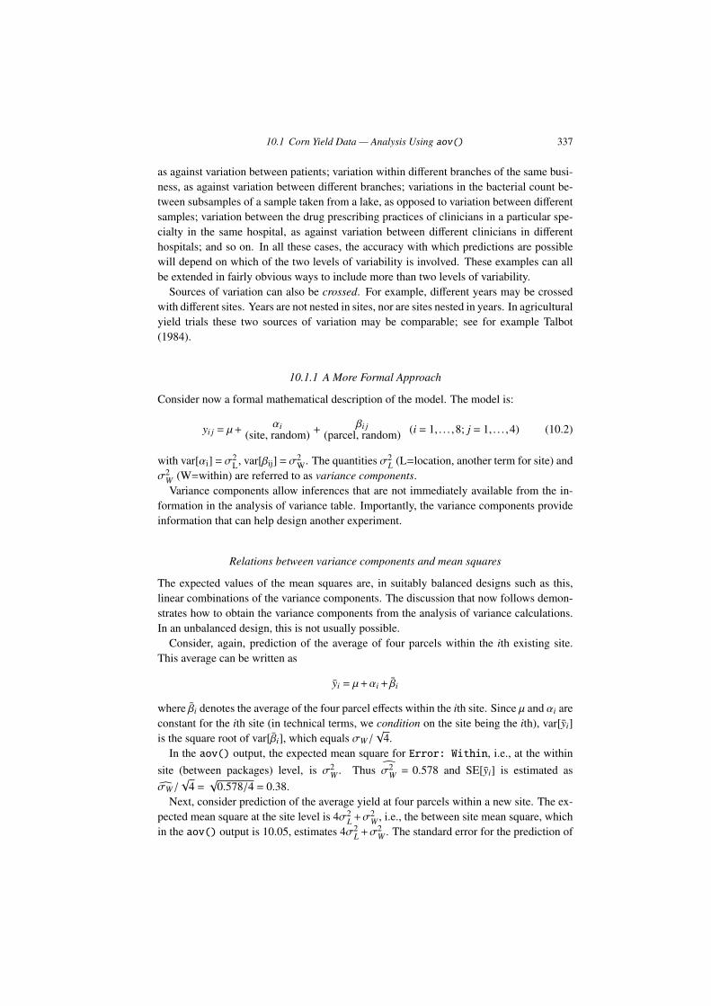
Figure 10.1: Corn yields for four parcels of land in each of eight sites on the Caribbean island ofAntigua. Data are in Table 10.1. They are a summarized version (parcel measurements are blockmeans) of a subset of data given in Andrews and Herzberg 1985, pp.339-353. Sites have beenreordered according to the magnitude of the site means.
The data set Orthodont that is used for the analyses of Subsection 10.7.2, and severaldata sets that appear in the exercises, are in the MEMSS package.
Corn yield measurements example
An especially simple multi-level model is the random e↵ects model for the one way layout.Thus, consider the data frame ant111b in the DAAG package, based on an agriculturalexperiment on the Caribbean island of Antigua. Corn yield measurements were taken onfour parcels of land within each of eight sites. Figure 10.1 is a visual summary.
Code for Figure 10.1 is:
library(lattice); library(DAAG)
Site <- with(ant111b, reorder(site, harvwt, FUN=mean))
stripplot(Site ˜ harvwt, data=ant111b, scales=list(tck=0.5),
xlab="Harvest weight of corn")
Figure 10.1 suggests that, as might be expected, parcels on the same site will be rela-tively similar, while parcels on di↵erent sites will be relatively less similar. A farmer whosefarm was close to one of the experimental sites might take data from that site as indicativeof what he/she might expect. In other cases it may be more appropriate for a farmer toregard his/her farm as a new site, distinct from the experimental sites, so that the issue isone of generalizing to a new site. Prediction for a new parcel at one of the existing sites ismore accurate than prediction for a totally new site.
There are two levels of random variation. They are site, and parcel within site. Variationbetween sites may be due, for example, to di↵erences in elevation or proximity to bodiesof water. Within a site, one might expect di↵erent parcels to be somewhat similar in termsof elevation and climatic conditions; however, di↵erences in soil fertility and drainage maystill have a noticeable e↵ect on yield. (Use of information on such e↵ects, not available aspart of the present data, might allow more accurate modeling.)
334 10. Multi-level Models, and Repeated Measures
The model will need: (a) a random term that accounts for variation within sites, and(b) a second superimposed random term that allows variability between parcels that areon di↵erent sites to be greater than variation between parcels within sites. The di↵erentrandom terms are known as random e↵ects.
The model can be expressed as:
yield = overall mean + site e↵ect(random) +
parcel e↵ect (within site)(random) (10.1)
Because of the balance (there are four parcels per site), analysis of variance using aov()is entirely satisfactory for these data. Section 10.1 that now follows will demonstrate theanalysis that uses aov().
It will then be instructive, in Subsection 10.2 below, to set set results from use of aov()alongside results from the function lmer() (from lme4). The comparison is between atraditional analysis of variance approach, which is fine for data from a balanced experi-mental design, and a general multi-level modeling approach that can in principle handleboth balanced and unbalanced designs.
10.1 Corn Yield Data — Analysis Using aov()
In the above model, the overall mean is assumed to be a fixed constant, while the site andparcel e↵ects are both assumed to be random. In order to account for the two levels ofvariation, the model formula must include an Error(site) term, thus:
library(DAAG)
ant111b.aov <- aov(harvwt ˜ 1 + Error(site), data=ant111b)
Explicit mention of the “within site” level of variation is unnecessary. (Use of the errorterm Error(site/parcel), which explicitly identifies parcels within sites, is howeverallowed.) Output is:
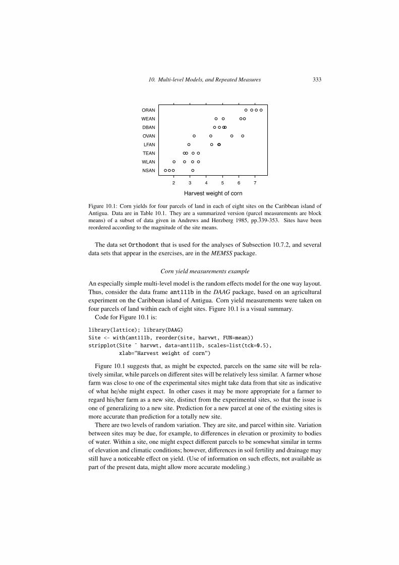
> summary(ant111b.aov)
Error: site
Df Sum Sq Mean Sq F value Pr(>F)
Residuals 7 70.34 10.05
Error: Within
Df Sum Sq Mean Sq F value Pr(>F)
Residuals 24 13.861 0.578
The analysis of variance (anova) table breaks the total sum of squares about the meaninto two parts – variation within sites, and variation between site means. Since there areeight sites, the variation between sites is estimated from seven degrees of freedom, afterestimating the overall mean. Within each site, estimation of the site mean leaves threedegrees of freedom for estimating the variance for that site. Three degrees of freedom ateach of eight sites yields 24 degrees of freedom for estimating within site variation.
10.1 Corn Yield Data — Analysis Using aov() 335
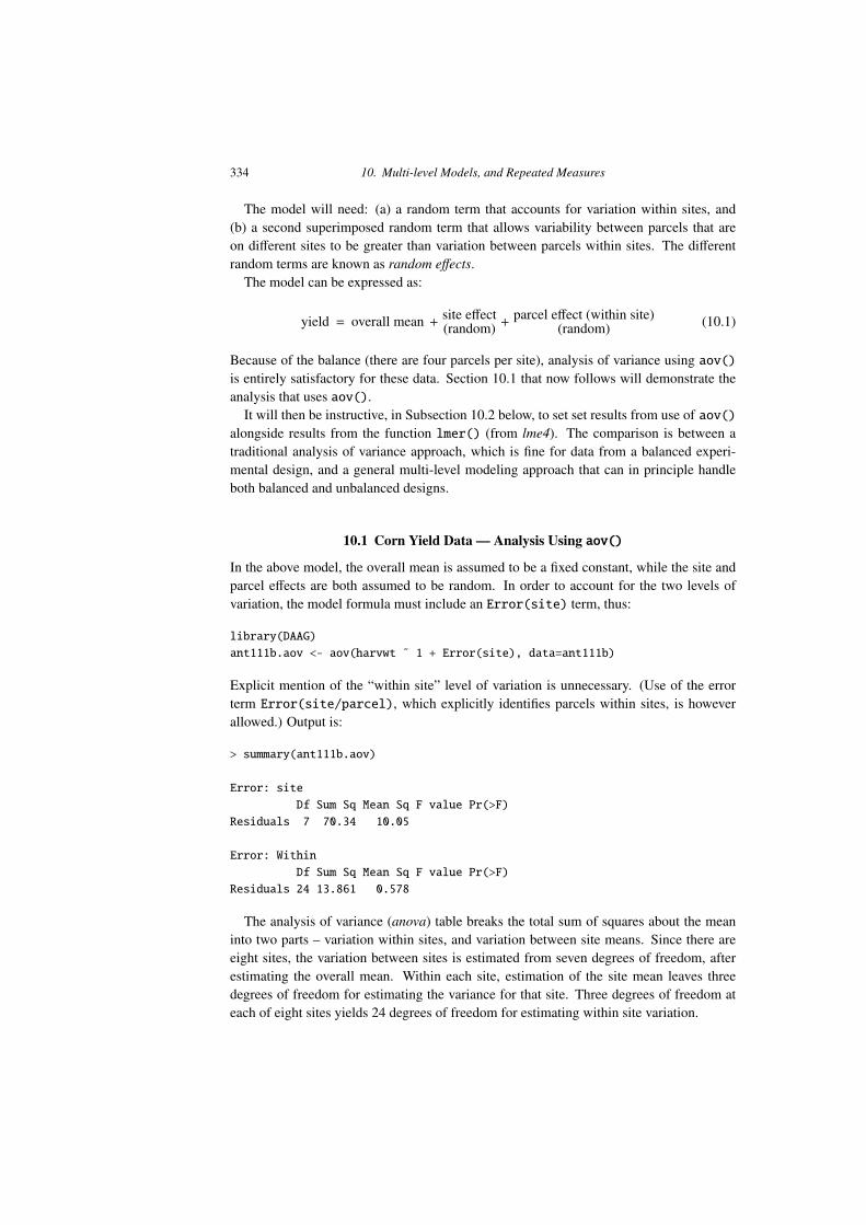
Table 10.1: The leftmost column has harvest weights (harvwt), for theparcels in each site, for the Antiguan corn data. Each of these harvestweights can be expressed as the sum of the overall mean (= 4.29), sitee↵ect (fourth column), and residual from the site e↵ect (final column).The information in the fourth and final columns can be used to generatethe sums of squares and mean squares for the analysis of variancetable.
Site Parcel measurements Site Residuals frommeans e↵ects site mean
DBAN 5.16, 4.8, 5.07, 4.51 4.88 +0.59 0.28, �0.08, 0.18, �0.38LFAN 2.93, 4.77, 4.33, 4.8 4.21 �0.08 �1.28, 0.56, 0.12, 0.59NSAN 1.73, 3.17, 1.49, 1.97 2.09 �2.2 �0.36, 1.08, �0.6, �0.12ORAN 6.79, 7.37, 6.44, 7.07 6.91 +2.62 �0.13, 0.45, �0.48, 0.15OVAN 3.25, 4.28, 5.56, 6.24 4.83 +0.54 �1.58, �0.56, 0.73, 1.4TEAN 2.65, 3.19, 2.79, 3.51 3.03 �1.26 �0.39, 0.15, �0.25, 0.48
WEAN 5.04, 4.6, 6.34, 6.12 5.52 +1.23 �0.49, �0.93, 0.81, 0.6WLAN 2.02, 2.66, 3.16, 3.52 2.84 �1.45 �0.82, �0.18, 0.32, 0.68
Interpreting the mean squares
The division of the sum of squares into two parts mirrors the two di↵erent types of predic-tion that can be based on these data.
First, suppose that measurements are taken on four new parcels at one of the existingsites. How much might the mean of the four measurements be expected to vary, betweenone such set of measurements and another. For this, the only source of uncertainty is parcelto parcel variation within the existing site. Recall that standard errors of averages can beestimated by dividing the (within) residual mean square by the sample size (in this case,four), and taking the square root. Thus the relevant standard error is
p0.578/4 = 0.38.
(Note that this is another form of the pooled variance estimate discussed in Chapter 4.)Second, for prediction of an average of four parcels at some di↵erent site, distinct from
the original eight, the relevant standard error can be calculated in the same way, but usingthe between site mean square; it is
p10.05/4 = 1.6.
Details of the calculations
This subsection may be omitted by readers who already understand the mean square calcu-lations. Table 10.1 contains the data and gives an indication of the mean square calculationsused to produce the anova table.
First, the overall mean is calculated. It is 4.29 for this example. Then site means arecalculated using the parcel measurements. Site e↵ects are calculated by subtracting theoverall mean from the site means. The parcel e↵ects are the residuals after subtracting thesite means from the individual parcel measurements.
The between site sum of squares is obtained by squaring the site e↵ects, summing, andmultiplying by four. This last step reflects the number of parcels per site. Dividing by thedegrees of freedom (8 - 1 = 7) gives the mean square.

336 10. Multi-level Models, and Repeated Measures
The within site sum of squares is obtained by squaring the residuals (parcel e↵ects),summing, and dividing by the degrees of freedom (8 ⇥ (4-1) = 24).
Practical use of the analysis of variance results
Treating site as random when we do the analysis does not at all commit us to treating it asrandom for purposes of predicting results from a new site. Rather, it allows us this option,if this seems appropriate. Consider how a person who has newly come to the island, andintends to purchase a farming property, might assess the prospects of a farming propertythat is available for purchase. Two extremes in the range of possibilities are:
1. The property is similar to one of the sites for which data are available, so similar infact that yields would be akin to those from adding new parcels that together comprisethe same area on that site.
2. It is impossible to say with any assurance where the new property should be placedwithin the range of results from experimental sites. The best that can be done is totreat it as a random sample from the population of all possible sites on the island.
Given adequate local knowledge (and ignoring changes that have taken place since thesedata were collected!) it might be possible to classify most properties on the island as likelyto give yields that are relatively close to those from one or more of the experimental sites.Given such knowledge, it is then possible to give a would-be purchaser advice that is morefinely tuned. The standard error (for the mean of four parcels) is likely to be much less than1.6, and may for some properties be closer to 0.38. In order to interpret analysis results withconfidence, and give the would-be purchaser high quality advice, a fact-finding mission tothe island of Antigua may be expedient!
Random e↵ects vs. fixed e↵ects
The random e↵ects model bears some resemblance to the one way model considered inSection 4.5. The important di↵erence is that in Section 4.5 the interest was in di↵erencesbetween the fixed levels of the nutrient treatment that were used in the experiment. Gener-alization to other possible nutrient treatments was not of interest, and would not have madesense. The only predictions that were possible were for nutrient treatments considered inthe study.
The random e↵ects model allows for predictions at two levels: (1) for agricultural yieldat a new location within an existing site, or (2) for locations in sites that were di↵erentfrom any of the sites that were included in the original study.
Nested factors – a variety of applications
Random e↵ects models apply in any situation where there is more than one level of randomvariability. In many situations, one source of variability is nested within the other – thusparcels are nested within sites.
Other examples include: variation between houses in the same suburb, as against varia-tion between suburbs, variation between di↵erent clinical assessments of the same patients,
10.1 Corn Yield Data — Analysis Using aov() 337
as against variation between patients; variation within di↵erent branches of the same busi-ness, as against variation between di↵erent branches; variations in the bacterial count be-tween subsamples of a sample taken from a lake, as opposed to variation between di↵erentsamples; variation between the drug prescribing practices of clinicians in a particular spe-cialty in the same hospital, as against variation between di↵erent clinicians in di↵erenthospitals; and so on. In all these cases, the accuracy with which predictions are possiblewill depend on which of the two levels of variability is involved. These examples can allbe extended in fairly obvious ways to include more than two levels of variability.
Sources of variation can also be crossed. For example, di↵erent years may be crossedwith di↵erent sites. Years are not nested in sites, nor are sites nested in years. In agriculturalyield trials these two sources of variation may be comparable; see for example Talbot(1984).
10.1.1 A More Formal Approach
Consider now a formal mathematical description of the model. The model is:
yi j = µ+↵i
(site, random) +�i j
(parcel, random) (i = 1, . . . ,8; j = 1, . . . ,4) (10.2)
with var[↵i] =�2L, var[�ij] =�2
W. The quantities �2L (L=location, another term for site) and
�2W (W=within) are referred to as variance components.Variance components allow inferences that are not immediately available from the in-
formation in the analysis of variance table. Importantly, the variance components provideinformation that can help design another experiment.
Relations between variance components and mean squares
The expected values of the mean squares are, in suitably balanced designs such as this,linear combinations of the variance components. The discussion that now follows demon-strates how to obtain the variance components from the analysis of variance calculations.In an unbalanced design, this is not usually possible.
Consider, again, prediction of the average of four parcels within the ith existing site.This average can be written as
yi = µ+↵i+ �i
where �i denotes the average of the four parcel e↵ects within the ith site. Since µ and ↵i areconstant for the ith site (in technical terms, we condition on the site being the ith), var[yi]is the square root of var[�i], which equals �W/
p4.
In the aov() output, the expected mean square for Error: Within, i.e., at the withinsite (between packages) level, is �2
W . Thus c�2W = 0.578 and SE[yi] is estimated as
c�W/p
4 =p
0.578/4 = 0.38.Next, consider prediction of the average yield at four parcels within a new site. The ex-
pected mean square at the site level is 4�2L+�
2W , i.e., the between site mean square, which
in the aov() output is 10.05, estimates 4�2L+�
2W . The standard error for the prediction of
338 10. Multi-level Models, and Repeated Measures
the average yield at four parcels within a new site isq�2
L +�2W/4 =
q(4�2
L +�2W )/4
The estimate for this isp
10.05/4 = 1.59.Finally, note how, in this balanced case, �2
L can be estimated from the analysis of vari-ance output. Equating the expected between site mean square to the observed mean square:
4c�2L +
c�2W = 10.05,
i.e.,
4c�2L +0.578 = 10.05,
so that c�2L = (10.05-0.578)/4 = 2.37.
Interpretation of variance components
In summary, here is how the variance components can be interpreted, for the Antiguandata. Plugging in numerical values ( c�2
W = 0.578 and c�2L = 2.37), take-home messages
from this analysis are:
o For prediction for a new parcel at one of the existing sites, the standard error is c�W =p0.578 = 0.76
o For prediction for a new parcel at a new site, the standard error isq�2
L +�2W =p
2.37+0.578 = 1.72o For prediction of the mean of n parcels at a new site, the standard error isq
�2L +�
2W/n =
p2.37+0.578/n
[Notice that while �2W is divided by n, �2
L is not. This is because the site e↵ect is thesame for all n parcels.]
o For prediction of the total of n parcels at a new site, the standard error isq�2
Ln+�2W =p
2.37n+0.578
Additionally
• The variance of the di↵erence between two such parcels at the same site is 2�2W
[Both parcels have the same site e↵ect ↵i, so that var(↵i) does not contribute to thevariance of the di↵erence.]
• The variance of the di↵erence between two parcels that are in di↵erent sites is
2(�2L +�
2W )
Thus, where there are multiple levels of variation, the predictive accuracy can be dramat-ically di↵erent, depending on what is to be predicted. Similar issues arise in repeatedmeasures contexts, and in time series.
10.2 Analysis using lmer(), from the lme4 package 339
Intra-class correlation
According to the model, two observations at di↵erent sites are uncorrelated. Two observa-tions at the same site are correlated, by an amount that has the name intra-class correlationcorrelation. Here, it equals �2
L/(�2L +�
2W ). This is the proportion of residual variance
explained by di↵erences between sites.Plugging in the variance component estimates, the intra-class correlation for the corn
yield data is 2.37/(2.37+ 0.578) = .804. Roughly 80% of the yield variation is due todi↵erences between sites.
10.2 Analysis using lmer(), from the lme4 package
In output from the function lmer(), the assumption of two nested random e↵ects, i.e., ahierarchy of three levels of variation, is explicit. Variation between sites (this appearedfirst in the anova table in Subsection 10.1) is the “lower” of the two levels. Here, the nlmeconvention will be followed, and this will be called level 1. Variation between parcels inthe same site (this appeared second in the anova table, under “Residuals”) is at the “higher”of the two levels, conveniently called level 2.
The modeling command takes the form:
library(lme4)
ant111b.lmer <- lmer(harvwt ˜ 1 + (1 | site), data=ant111b)
The only fixed e↵ect is the overall mean. The (1 | site) term fits random variationbetween sites. Variation between the individual units that are nested within sites, i.e.,between parcels, are by default treated as random. Here is the default output:
> ## Note that there is no degrees of freedom information.
> print(ant111b.lmer, ranef.comp="Variance", digits=3)
Linear mixed model fit by REML ['lmerMod']
Formula: harvwt ˜ 1 + (1 | site)
Data: ant111b
REML criterion at convergence: 94.4163
Random effects:
Groups Name Variance
site (Intercept) 2.368
Residual 0.578
Number of obs: 32, groups: site, 8
Fixed Effects:
(Intercept)
4.29
Observe that, according to lmer(), c�2W = 0.578, and c�2
L = 2.368. Observe also that c�2W
= 0.578 is the mean square from the analysis of variance table. The mean square at level 1does not appear in the output from the lmer() analysis.
340 10. Multi-level Models, and Repeated Measures
The processing of output from lmer()
The function coef() will be used, with output from summary(), to obtain estimates offixed e↵ect coe�cients and their standard errors. Thus, for the model ant111b.lmer, weobtain:
> print(coef(summary(ant111b.lmer)), digits=3)
Estimate Std. Error t value
(Intercept) 4.29 0.56 7.66
Users who require approximate p-values can use the function mixed() from the afexpackage. A call to mixed() replaces the call to lmer(). This uses abilities fromthe pbkrtest package to process output from lmer(). If called with method="KR", theKenward-Roger approximation is used to calculate degrees of freedom for statistics in thet value column in the output from lmer(). With degrees of freedom thus given, thet-values are treated as t statistics and approximate p-values determined.
Objects returned by the function lmer() have the class merMod. Objects returned by thesummary()method for merMod objects have class summary.merMod. Objects returned byVarCorr(), used in the sequel for extracting variance component estimates, have classVarCorr.merMod.
See (help(merMod) for details of methods for merMod and summary.merMod objects.Note in particular the print() methods, with arguments that control the details of what iaprinted.1
Fitted values and residuals in lmer()
In hierarchical multi-level models, fitted values can be calculated at each level of variationthat the model allows. Corresponding to each level of fitted values, there is a set of residualsthat is obtained by subtracting the fitted values from the observed values.
The default, and at the time of writing the only option, is to calculate fitted values andresiduals that adjust for all random e↵ects except the residual. Here, these are estimatesof the site expected values. They di↵er slightly from the site means, as will be seen be-low. Such fitted values are known as BLUPs (Best Linear Unbiased Predictors). Amonglinear unbiased predictors of the site means, the BLUPs are designed to have the smallestexpected error mean square.
Relative to the site means yi., the BLUPs are pulled in toward the overall mean y... Themost extreme site means will on average, because of random variation, be more extremethan the corresponding “true” means for those sites. For the simple model considered here,the fitted value b↵i for the ith site is given by
byi. = y..+nc�2
L
nc�2L +
c�2W
(yi.� y..).
Shrinkage is substantial, i.e., a shrinkage factor much less than 1.0, when n�1 c�2W is large
1Thus, for use of print() with merMod and summary.merMod objects, the argument ranef.comp can be set to anycombination of comp="Variance" and comp="Std.Dev.". For use of print() with VarCorr.merMod objects, the samealternatives are available for the comp argument.
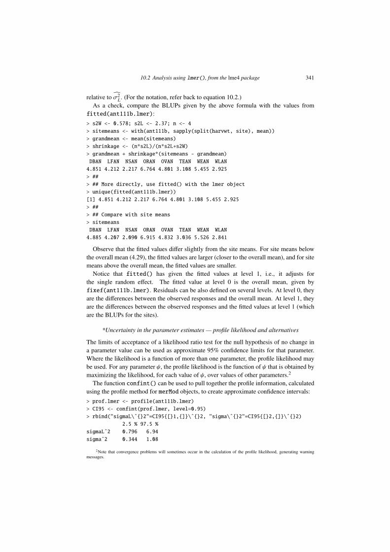
10.2 Analysis using lmer(), from the lme4 package 341
relative to c�2L. (For the notation, refer back to equation 10.2.)
As a check, compare the BLUPs given by the above formula with the values fromfitted(ant111b.lmer):> s2W <- 0.578; s2L <- 2.37; n <- 4
> sitemeans <- with(ant111b, sapply(split(harvwt, site), mean))
> grandmean <- mean(sitemeans)
> shrinkage <- (n*s2L)/(n*s2L+s2W)
> grandmean + shrinkage*(sitemeans - grandmean)
DBAN LFAN NSAN ORAN OVAN TEAN WEAN WLAN
4.851 4.212 2.217 6.764 4.801 3.108 5.455 2.925
> ##
> ## More directly, use fitted() with the lmer object
> unique(fitted(ant111b.lmer))
[1] 4.851 4.212 2.217 6.764 4.801 3.108 5.455 2.925
> ##
> ## Compare with site means
> sitemeans
DBAN LFAN NSAN ORAN OVAN TEAN WEAN WLAN
4.885 4.207 2.090 6.915 4.832 3.036 5.526 2.841
Observe that the fitted values di↵er slightly from the site means. For site means belowthe overall mean (4.29), the fitted values are larger (closer to the overall mean), and for sitemeans above the overall mean, the fitted values are smaller.
Notice that fitted() has given the fitted values at level 1, i.e., it adjusts forthe single random e↵ect. The fitted value at level 0 is the overall mean, given byfixef(ant111b.lmer). Residuals can be also defined on several levels. At level 0, theyare the di↵erences between the observed responses and the overall mean. At level 1, theyare the di↵erences between the observed responses and the fitted values at level 1 (whichare the BLUPs for the sites).
*Uncertainty in the parameter estimates — profile likelihood and alternatives
The limits of acceptance of a likelihood ratio test for the null hypothesis of no change ina parameter value can be used as approximate 95% confidence limits for that parameter.Where the likelihood is a function of more than one parameter, the profile likelihood maybe used. For any parameter , the profile likelihood is the function of that is obtained bymaximizing the likelihood, for each value of , over values of other parameters.2
The function confint() can be used to pull together the profile information, calculatedusing the profile method for merMod objects, to create approximate confidence intervals:> prof.lmer <- profile(ant111b.lmer)
> CI95 <- confint(prof.lmer, level=0.95)
> rbind("sigmaL\ˆ{}2"=CI95{[}1,{]}\ˆ{}2, "sigma\ˆ{}2"=CI95{[}2,{]}\ˆ{}2)
2.5 % 97.5 %
sigmaLˆ2 0.796 6.94
sigmaˆ2 0.344 1.08
2Note that convergence problems will sometimes occur in the calculation of the profile likelihood, generating warningmessages.
342 10. Multi-level Models, and Repeated Measures
ζ
−2
−1
0
1
2
1.0 1.5 2.0 2.5 3.0
σ1
0.6 0.8 1.0
σ
3 4 5 6
(Intercept)
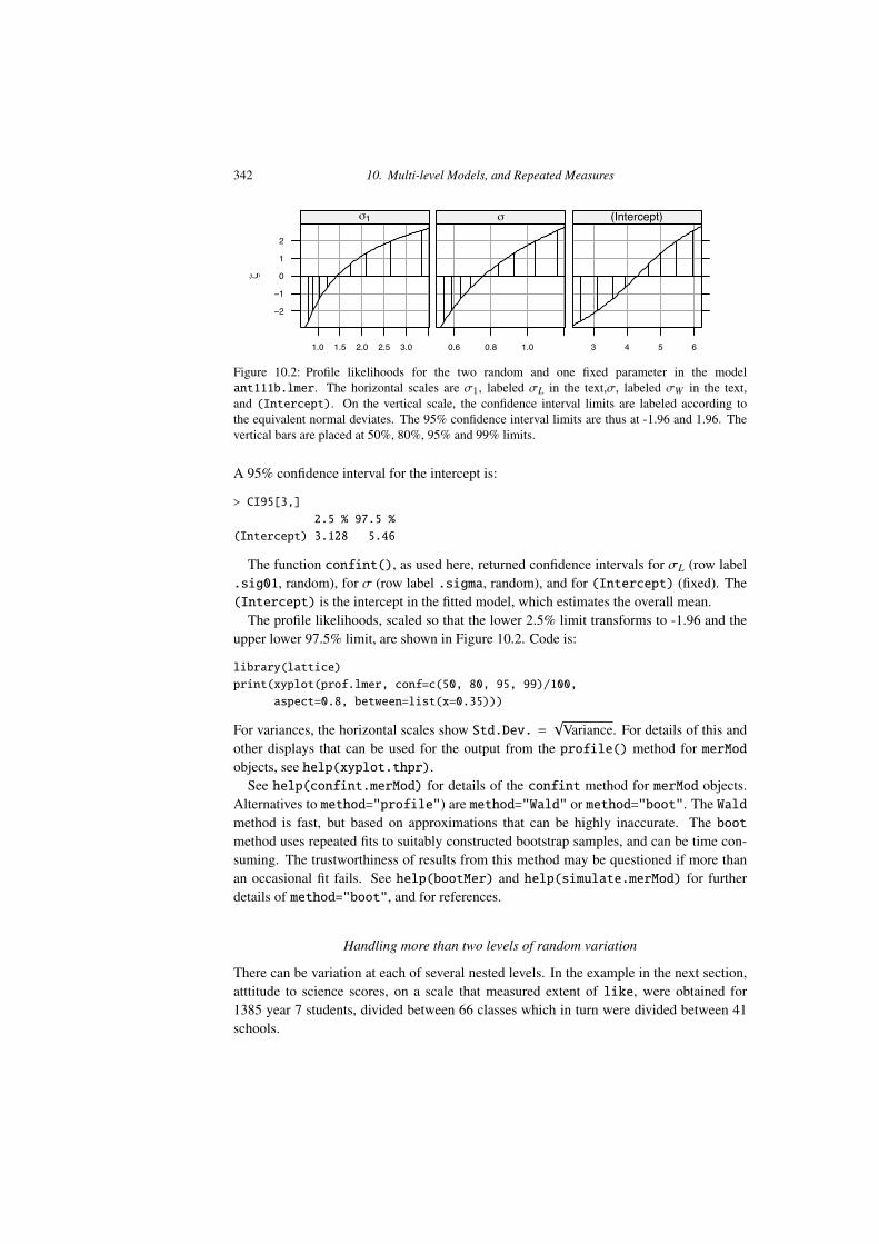
Figure 10.2: Profile likelihoods for the two random and one fixed parameter in the modelant111b.lmer. The horizontal scales are �1, labeled �L in the text,�, labeled �W in the text,and (Intercept). On the vertical scale, the confidence interval limits are labeled according tothe equivalent normal deviates. The 95% confidence interval limits are thus at -1.96 and 1.96. Thevertical bars are placed at 50%, 80%, 95% and 99% limits.
A 95% confidence interval for the intercept is:
> CI95[3,]
2.5 % 97.5 %
(Intercept) 3.128 5.46
The function confint(), as used here, returned confidence intervals for �L (row label.sig01, random), for � (row label .sigma, random), and for (Intercept) (fixed). The(Intercept) is the intercept in the fitted model, which estimates the overall mean.
The profile likelihoods, scaled so that the lower 2.5% limit transforms to -1.96 and theupper lower 97.5% limit, are shown in Figure 10.2. Code is:
library(lattice)
print(xyplot(prof.lmer, conf=c(50, 80, 95, 99)/100,
aspect=0.8, between=list(x=0.35)))
For variances, the horizontal scales show Std.Dev. =p
Variance. For details of this andother displays that can be used for the output from the profile() method for merModobjects, see help(xyplot.thpr).
See help(confint.merMod) for details of the confint method for merMod objects.Alternatives to method="profile") are method="Wald" or method="boot". The Waldmethod is fast, but based on approximations that can be highly inaccurate. The bootmethod uses repeated fits to suitably constructed bootstrap samples, and can be time con-suming. The trustworthiness of results from this method may be questioned if more thanan occasional fit fails. See help(bootMer) and help(simulate.merMod) for furtherdetails of method="boot", and for references.
Handling more than two levels of random variation
There can be variation at each of several nested levels. In the example in the next section,atttitude to science scores, on a scale that measured extent of like, were obtained for1385 year 7 students, divided between 66 classes which in turn were divided between 41schools.
10.3 Survey Data, with Clustering 343
●
●
private
public
2 3 4 5 6
Class average of score
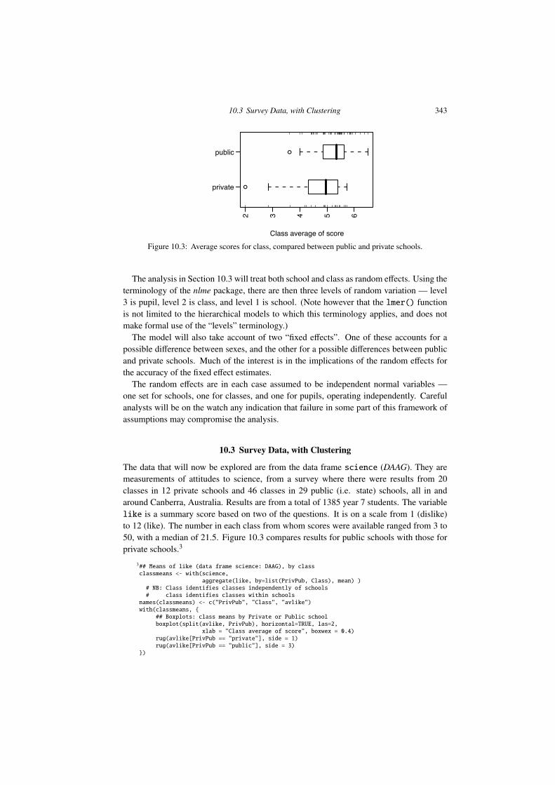
Figure 10.3: Average scores for class, compared between public and private schools.
The analysis in Section 10.3 will treat both school and class as random e↵ects. Using theterminology of the nlme package, there are then three levels of random variation — level3 is pupil, level 2 is class, and level 1 is school. (Note however that the lmer() functionis not limited to the hierarchical models to which this terminology applies, and does notmake formal use of the “levels” terminology.)
The model will also take account of two “fixed e↵ects”. One of these accounts for apossible di↵erence between sexes, and the other for a possible di↵erences between publicand private schools. Much of the interest is in the implications of the random e↵ects forthe accuracy of the fixed e↵ect estimates.
The random e↵ects are in each case assumed to be independent normal variables —one set for schools, one for classes, and one for pupils, operating independently. Carefulanalysts will be on the watch any indication that failure in some part of this framework ofassumptions may compromise the analysis.
10.3 Survey Data, with Clustering
The data that will now be explored are from the data frame science (DAAG). They aremeasurements of attitudes to science, from a survey where there were results from 20classes in 12 private schools and 46 classes in 29 public (i.e. state) schools, all in andaround Canberra, Australia. Results are from a total of 1385 year 7 students. The variablelike is a summary score based on two of the questions. It is on a scale from 1 (dislike)to 12 (like). The number in each class from whom scores were available ranged from 3 to50, with a median of 21.5. Figure 10.3 compares results for public schools with those forprivate schools.3
3## Means of like (data frame science: DAAG), by classclassmeans <- with(science,
aggregate(like, by=list(PrivPub, Class), mean) )# NB: Class identifies classes independently of schools# class identifies classes within schools
names(classmeans) <- c("PrivPub", "Class", "avlike")with(classmeans, {
## Boxplots: class means by Private or Public schoolboxplot(split(avlike, PrivPub), horizontal=TRUE, las=2,
xlab = "Class average of score", boxwex = 0.4)rug(avlike[PrivPub == "private"], side = 1)rug(avlike[PrivPub == "public"], side = 3)
})
344 10. Multi-level Models, and Repeated Measures
10.3.1 Alternative models
Within any one school, we might have
y = class e↵ect + pupil e↵ect
where y represents the attitude measure.Within any one school, we might use a one-way analysis of variance to estimate and
compare class e↵ects. However, this study has the aim of generalizing beyond the classesin the study to all of some wider population of classes, not just in the one school, but in awider population of schools from which the schools in the study were drawn. In order to beable to generalize in this way, we treat school (school), and class (class) within school,as random e↵ects. We are interested in possible di↵erences between the sexes (sex), andbetween private and public schools (PrivPub). The two sexes are not a sample from somelarger population of possible sexes (!), nor are the two types of school (for this study atleast) a sample from some large population of types of school. Thus they are fixed e↵ects.The interest is in the specific fixed di↵erences between males and females, and betweenprivate and public schools.
The preferred approach is a multi-level model analysis. While it is sometimes possibleto treat such data using an approximation to the analysis of variance as for a balancedexperimental design, it may be hard to know how good the approximation is. We specifysex (sex) and school type (PrivPub) as fixed e↵ects, while school (school) and class(class) are specified as random e↵ects. Class is nested within school; within each schoolthere are several classes. The model is
y =sex e↵ect
(fixed)+
type (private or public)(fixed)
+school e↵ect
(random)+
class e↵ect(random)
+pupil e↵ect(random).
Questions we might ask are:
• Are there di↵erences between private and public schools?• Are there di↵erences between females and males?• Clearly there are di↵erences among pupils. Are there di↵erences between classes
within schools, and between schools, greater than pupil to pupil variation within classeswould lead us to expect?
science.lmer <- lmer(like ˜ sex + PrivPub + (1 | school) +
(1 | school:class), data = science,
na.action=na.exclude)
The components of variance estimates are:
> print(VarCorr(science.lmer), comp="Variance", digits=3)
Groups Name Variance
school:class (Intercept) 0.321
school (Intercept) 0.000
Residual 3.052
The table of estimates and standard errors for the coe�cients of the fixed component issimilar to that from an lm() (single level) analysis.
10.3 Survey Data, with Clustering 345
> print(coef(summary(science.lmer)), digits=2)
Estimate Std. Error t value
(Intercept) 4.72 0.162 29.1
sexm 0.18 0.098 1.9
PrivPubpublic 0.41 0.186 2.2
Groups within the 1383 observations that are included are:
> summary(science.lmer)$ngrps
school:class school
66 41
Degrees of freedom are as follows:
• Between types of school: 41 (number of schools) - 2 = 39• Between sexes: 1383 - 1 (overall mean) - 1 (di↵erences between males and females) -
65 (di↵erences between the 66 school:class combinations) = 1316
The comparison between types of schools compares 12 private schools with 29 publicschools, comprising 41 algebraically independent items of information. However becausethe numbers of classes and class sizes di↵er between schools, the three components ofvariance contribute di↵erently to these di↵erent accuracies, and the 39 degrees of freedomare for a statistic that has only an approximate t-distribution. On the other hand, schoolsare made up of mixed males and female classes. The between pupils level of variation,where the only component of variance is that for the Residual in the output above, isthus the relevant level for the comparison between males and females. The t-test for thiscomparison is, under model assumptions, an exact test with 1316 degrees of freedom.
There are three variance components:
Between schools (school) 0.000Between classes (school:class) 0.321Between students (Residual) 3.052
It is important to note that these variances form a nested hierarchy. Variation betweenstudents contributes to variation between classes. Variation between students and betweenclasses both contribute to variation between schools. The modest-sized between class com-ponent of variance tells us that di↵erences between classes are greater than would be ex-pected from di↵erences between students alone. This will be further discussed shortly.
As the estimate for the between schools component of variance is zero, it can be omit-ted from the model, leading to the following simpler analysis. Notice that the variancecomponent estimates are, to three decimal places, the same as before:
science1.lmer <- lmer(like ˜ sex + PrivPub + (1 | school:class),
data = science, na.action=na.exclude)
Estimates of random and fixed e↵ects are:
> print(VarCorr(science1.lmer), comp="Variance", digits=3)
Groups Name Variance
school:class (Intercept) 0.321
346 10. Multi-level Models, and Repeated Measures
Residual 3.052
> print(coef(summary(science1.lmer)), digits=2)
Estimate Std. Error t value
(Intercept) 4.72 0.162 29.1
sexm 0.18 0.098 1.9
PrivPubpublic 0.41 0.186 2.2
Approximate p-values, if required, can be obtained thus:
> library(afex)
> mixed(like ˜ sex + PrivPub + (1 | school:class),
data = na.omit(science), method="KR")
Contrasts set to contr.sum for the following variables: sex, PrivPub, school, class
. . . .
Effect F ndf ddf F.scaling p.value
1 sex 3.44 1 1379.49 1.00 .06
2 PrivPub 4.91 1 60.44 1.00 .03
In the output, ddf is an acronym for “denominator degrees of freedom”.
More detailed examination of the output
Now use the function confint() to get approximate 95% confidence intervals for thevariance components:
> ## Use profile likelihood
> pp <- profile(science1.lmer, which="theta_")
> # which="theta_": all random parameters
> # which="beta_": fixed effect parameters
> var95 <- confint(pp, level=0.95)ˆ2
> # Square to get variances in place of SDs
> rownames(var95) <- c("sigma_Classˆ2", "sigmaˆ2")
> signif(var95, 3)
2.5 % 97.5 %
sigma_Classˆ2 0.178 0.511
sigmaˆ2 2.830 3.300
To what extent do di↵erences between classes a↵ect the attitude to science? A mea-sure of the e↵ect is the intra-class correlation, which is the proportion of variance that isexplained by di↵erences between classes. Here, it equals 0.321/(0.321+ 3.052) = 0.095.The main influence comes from outside the class that the pupil attends, e.g. from home,television, friends, inborn tendencies, etc.
Do not be tempted to think that, because 0.321 is small relative to the within classcomponent variance of 3.05, it is of little consequence. The variance for the mean of aclass that is chosen at random is 0.321 + 3.05/n. Thus, with a class size of 20, the betweenclass component makes a bigger contribution than the within class component. If all classeswere the same size, then the standard error of the di↵erence between class means for publicschools and those for private schools would, as there were 20 private schools and 46 public
10.3 Survey Data, with Clustering 347
●
●
●
●
●●
●
●●
●
●
●●●
●●
●●●
●−1
.00.
01.
0
# in class (square root scale)
Estim
ate
of c
lass
effe
ct
10 20 30 50
A
●
●
●
●
●●
●
●
●
●
●
●●
●
●
●
●
●
●
●23
45
6
# in class (square root scale)
With
in c
lass
var
ianc
e
10 20 30 50
B
●
●●
●
●
●
●
●
●
●
●●●
●●
●
●
●
●
●
●
●
●
●
●
●
●
●
●
●●
●
●
●
●
●
●●
●
●●
●
●
●
●
●
●●
●
●●●
●
●●
●
●
●●●
●●
●●●
●
−2 −1 0 1 2
−1.0
0.0
1.0
Theoretical Quantiles
Ord
ered
site
effe
cts
C
●
●
●
●
●
●
●
●
●
●
●
●
●
●
●
●●●
●
●
●●●
●
●
●
●●
●
●
●
●●
●●
●
●
●
●
●
●●
●●
●
●
●
●
●
●●
●
●
●
●
●
●
●
●
●
●
●
●
●
●
●●
●
●
●
●
●
●
●
●
●
●
●
●
●
●
●
●
●●
●
●
●
●
●●
●
●●
●
●
●
●
●●
●
●
●
●
●
●
●
●
●
●
●
●
●
●
●
●
●
●●●●
●
●
●●
●
●
●●
●
●
●
●
●●●
●
●
●
●●
●
●
●
●●
●
●
●●
●
●
●
●
●
●
●●
●●
●
●
●
●
●
●
●
●
●
●
●●
●
●
●
●
●
●●●●
●
●
●●●●●●●
●
●
●
●●
●●
●
●●●
●
●●
●
●
●
●
●
●
●
●
●●
●
●
●
●
●●
●●
●
●●
●
●
●
●●
●
●
●
●
●●●
●
●
●
●
●
●●
●
●●
●
●
●
●
●
●
●
●
●
●
●
●
●●
●
●
●
●
●●
●●
●
●
●
●
●
●
●
●
●
●●
●
●
●
●
●
●
●●●●●●
●
●
●●
●
●
●
●
●●
●
●
●
●
●
●
●●
●●
●
●
●
●
●●
●
●
●
●●
●
●
●
●
●
●
●
●
●
●●
●
●
●●
●
●
●
●
●
●
●
●
●
●
●
●
●
●
●
●●●●●
●●●●
●
●
●
●●
●
●
●●
●
●
●
●●
●
●
●
●
●
●
●
●
●
●
●
●●
●
●
●●●
●
●●
●
●
●
●
●
●●
●
●
●
●
●
●
●
●
●
●
●●
●
●
●●●●
●
●
●
●
●
●
●
●
●
●
●
●
●●●
●
●
●●
●
●
●●
●
●
●
●
●
●●
●
●
●
●
●●●
●
●
●●
●
●
●
●●
●
●
●●
●
●
●
●
●
●
●
●
●
●●
●
●
●
●
●
●
●
●●
●
●●
●
●
●●
●
●
●
●
●
●
●
●
●
●
●
●
●
●
●
●●
●●
●
●
●
●
●
●
●
●●●●●
●
●
●
●
●
●●●
●
●
●
●
●●
●
●
●
●
●
●
●●
●
●
●
●
●
●
●●
●●
●
●
●●●●
●
●
●
●
●●
●
●
●
●
●
●
●●●
●
●
●
●
●
●
●●
●
●
●
●
●
●●
●
●
●
●
●
●
●●
●
●
●
●
●●
●
●
●
●●
●●
●
●●
●●●
●
●
●●
●
●
●
●●
●
●
●
●
●
●
●
●
●
●
●
●●●●
●
●
●
●
●
●
●
●●●
●
●
●
●
●
●
●
●●
●
●
●●
●
●
●
●
●●
●●
●
●
●
●
●
●
●
●
●
●
●●
●
●●
●
●
●
●
●
●
●
●
●
●
●●
●
●
●●
●
●
●●
●
●
●
●
●
●
●
●
●
●
●
●
●
●
●●
●
●
●
●●●
●
●
●
●
●
●
●
●
●
●
●
●
●
●
●
●
●
●
●
●
●
●
●
●
●
●
●
●
●
●
●●
●
●
●
●
●●
●●
●
●
●
●
●
●
●
●
●
●
●
●
●
●
●
●
●
●
●
●
●
●
●
●
●
●
●
●
●
●
●
●●
●
●
●
●
●
●
●●
●
●
●
●
●
●
●
●●●●●
●
●
●
●●
●
●
●
●
●●
●
●
●
●
●
●
●
●
●
●
●
●
●
●
●●●
●
●
●
●
●●
●●
●
●
●●
●
●
●
●●
●
●
●
●
●
●
●
●
●●
●
●
●
●
●
●
●
●
●
●●
●
●●
●●
●
●●●●
●●
●
●
●●●
●
●
●
●
●
●
●
●●
●
●●
●
●●
●
●
●
●●
●
●●
●
●
●●
●
●
●
●
●
●●
●
●
●
●
●
●
●●
●
●
●
●
●
●
●
●
●
●
●●
●
●
●
●
●●
●
●
●
●
●
●
●
●
●
●
●
●
●
●
●
●
●
●
●
●
●
●
●
●
●
●
●
●●
●
●
●
●
●
●
●●
●
●
●
●●
●●
●
●
●
●●
●
●
●
●
●
●●●
●
●
●
●
●
●
●
●
●
●
●
●
●
●
●
●
●
●
●
●●
●
●
●
●
●
●●
●
●
●
●
●●
●
●
●
●
●●
●
●
●
●
●
●
●
●●●
●
●
●
●
●
●
●
●
●
●
●
●
●●
●
●
●
●
●●
●●
●
●
●●
●●
●
●
●
●
●●●
●
●
●
●
●●
●
●
●
●
●
●
●
●
●
●
●
●
●
●
●
●
●
●
●
●
●
●
●
●
●
●
●
●
●
●
●●
●
●
●●
●
●
●
●
●
●
●
●
●
●
●
●
●
●
●
●
●
●●●
●
●
●
●●
●
●
●●●
●●●
●
●
●
●
●●
●
●
●
●●
●
●
●
●
●●
●
●
●
●
●
●
●●
●
●
●
●
●
●
●●
●
●
●
●
●
●
●
●
●
●
●●●
●●
●●
●
●
●
●
●●
●●
●
●
●●
●
●
●
●
●
●
●●
●
●●
●●
●●
●
●
●●
●
●
●●●●
●●●
●
●
●
●
●
●
●
●
●
●
●
●●●●
●
●
●
●
●●
●
●
●
●
●●●
●
●●●●
●
●●
●
●
●
●
●
●●●●●●
●
●
●
●●
●
●
●
●
●
●●
●
●
●
●
●
●
●
●
●
●●
●●●
●
●
●
●
●
●
●
●
●
●
●
●
●●●●
●
●●●
●●
●
●
●
●
●
●
●
●
−3 −1 1 2 3
−40
24
Theoretical Quantiles
Ord
ered
w/i
class
resid
uals D
● Private Public
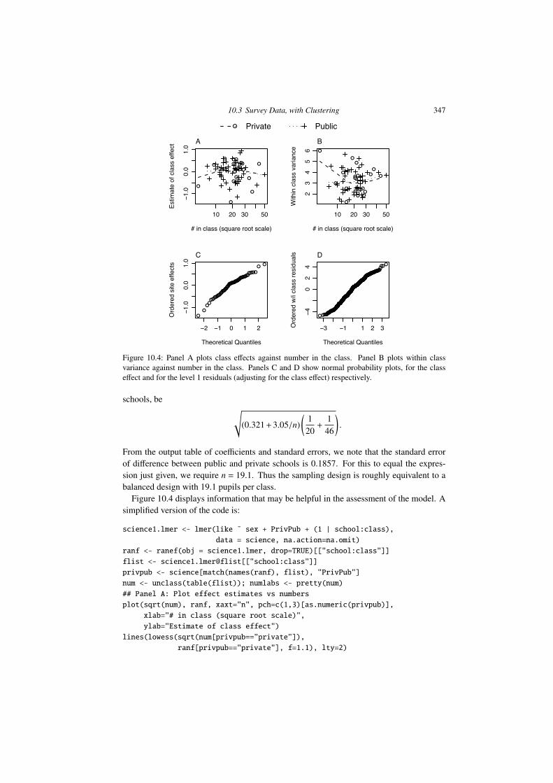
Figure 10.4: Panel A plots class e↵ects against number in the class. Panel B plots within classvariance against number in the class. Panels C and D show normal probability plots, for the classe↵ect and for the level 1 residuals (adjusting for the class e↵ect) respectively.
schools, bes
(0.321+3.05/n)
120+
146
!.
From the output table of coe�cients and standard errors, we note that the standard errorof di↵erence between public and private schools is 0.1857. For this to equal the expres-sion just given, we require n = 19.1. Thus the sampling design is roughly equivalent to abalanced design with 19.1 pupils per class.
Figure 10.4 displays information that may be helpful in the assessment of the model. Asimplified version of the code is:
science1.lmer <- lmer(like ˜ sex + PrivPub + (1 | school:class),
data = science, na.action=na.omit)
ranf <- ranef(obj = science1.lmer, drop=TRUE)[["school:class"]]
flist <- science1.lmer@flist[["school:class"]]
privpub <- science[match(names(ranf), flist), "PrivPub"]
num <- unclass(table(flist)); numlabs <- pretty(num)
## Panel A: Plot effect estimates vs numbers
plot(sqrt(num), ranf, xaxt="n", pch=c(1,3)[as.numeric(privpub)],
xlab="# in class (square root scale)",
ylab="Estimate of class effect")
lines(lowess(sqrt(num[privpub=="private"]),
ranf[privpub=="private"], f=1.1), lty=2)
348 10. Multi-level Models, and Repeated Measures
lines(lowess(sqrt(num[privpub=="public"]),
ranf[privpub=="public"], f=1.1), lty=3)
axis(1, at=sqrt(numlabs), labels=paste(numlabs))
res <- residuals(science1.lmer)
vars <- tapply(res, INDEX=list(flist), FUN=var)*(num-1)/(num-2)
## Panel B: Within class variance estimates vs numbers
plot(sqrt(num), vars, pch=c(1,3)[unclass(privpub)])
lines(lowess(sqrt(num[privpub=="private"]),
as.vector(vars)[privpub=="private"], f=1.1), lty=2)
lines(lowess(sqrt(num[privpub=="public"]),
as.vector(vars)[privpub=="public"], f=1.1), lty=3)
## Panel C: Normal probability plot of site effects
qqnorm(ranf, ylab="Ordered site effects", main="")
## Panel D: Normal probability plot of residuals
qqnorm(res, ylab="Ordered w/i class residuals", main="")
Panels A shows no clear evidence of a trend. Panel B perhaps suggests that variances maybe larger for the small number of classes that had more than about 30 students. PanelsC and D show distributions that seem acceptably close to normal. The interpretation ofpanel C is complicated by the fact that the di↵erent e↵ects are estimated with di↵erentaccuracies.
10.3.2 Instructive, though faulty, analyses
Ignoring class as the random e↵ect
It is important that the specification of random e↵ects be correct. It is enlightening to do ananalysis that is not quite correct, and investigate the scope that it o↵ers for misinterpreta-tion. We fit school, ignoring class, as a random e↵ect. The estimates of the fixed e↵ectschange little.> science2.lmer <- lmer(like ˜ sex + PrivPub + (1 | school),
+ data = science, na.action=na.exclude)
> science2.lmer
. . . .
Fixed effects:
Estimate Std. Error t value Pr(>|t|)
(Intercept) 4.738 0.163 29.00 <2e-16
sexm 0.197 0.101 1.96 0.051
PrivPubpublic 0.417 0.185 2.25 0.030
This analysis suggests, wrongly, that the between schools component of variance is sub-stantial. The estimated variance components are4
Between schools 0.166Between students 3.219
This is misleading. From our earlier investigation, it is clear that the di↵erence is betweenclasses, not between schools!
4print(VarCorr(science2.lmer), comp="Variance", digits=3)## The component of variance that is labeled 'Residual' is## the estimate of the within class variance.
10.4 A Multi-level Experimental Design 349
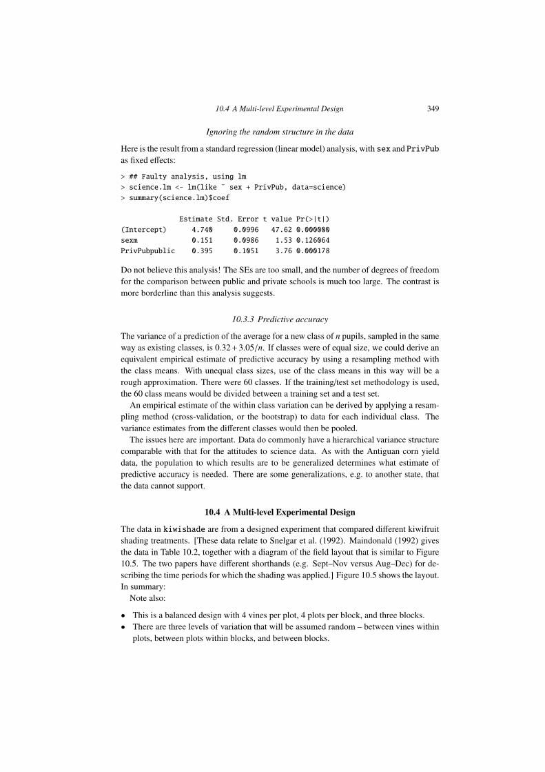
Ignoring the random structure in the data
Here is the result from a standard regression (linear model) analysis, with sex and PrivPubas fixed e↵ects:
> ## Faulty analysis, using lm
> science.lm <- lm(like ˜ sex + PrivPub, data=science)
> summary(science.lm)$coef
Estimate Std. Error t value Pr(>|t|)
(Intercept) 4.740 0.0996 47.62 0.000000
sexm 0.151 0.0986 1.53 0.126064
PrivPubpublic 0.395 0.1051 3.76 0.000178
Do not believe this analysis! The SEs are too small, and the number of degrees of freedomfor the comparison between public and private schools is much too large. The contrast ismore borderline than this analysis suggests.
10.3.3 Predictive accuracy
The variance of a prediction of the average for a new class of n pupils, sampled in the sameway as existing classes, is 0.32+3.05/n. If classes were of equal size, we could derive anequivalent empirical estimate of predictive accuracy by using a resampling method withthe class means. With unequal class sizes, use of the class means in this way will be arough approximation. There were 60 classes. If the training/test set methodology is used,the 60 class means would be divided between a training set and a test set.
An empirical estimate of the within class variation can be derived by applying a resam-pling method (cross-validation, or the bootstrap) to data for each individual class. Thevariance estimates from the di↵erent classes would then be pooled.
The issues here are important. Data do commonly have a hierarchical variance structurecomparable with that for the attitudes to science data. As with the Antiguan corn yielddata, the population to which results are to be generalized determines what estimate ofpredictive accuracy is needed. There are some generalizations, e.g. to another state, thatthe data cannot support.
10.4 A Multi-level Experimental Design
The data in kiwishade are from a designed experiment that compared di↵erent kiwifruitshading treatments. [These data relate to Snelgar et al. (1992). Maindonald (1992) givesthe data in Table 10.2, together with a diagram of the field layout that is similar to Figure10.5. The two papers have di↵erent shorthands (e.g. Sept–Nov versus Aug–Dec) for de-scribing the time periods for which the shading was applied.] Figure 10.5 shows the layout.In summary:
Note also:
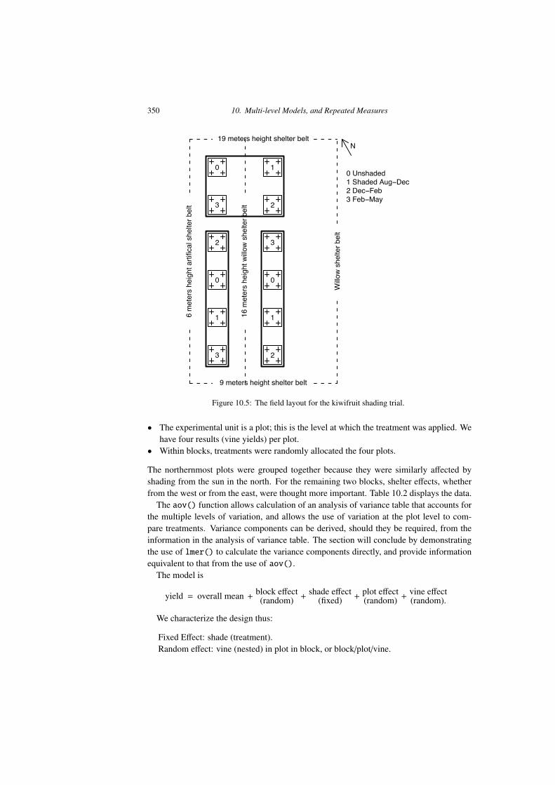
• This is a balanced design with 4 vines per plot, 4 plots per block, and three blocks.• There are three levels of variation that will be assumed random – between vines within
plots, between plots within blocks, and between blocks.
350 10. Multi-level Models, and Repeated Measures
3
1
0
2
2
1
0
3
3 2
10
6 m
eter
s he
ight
arti
fical
she
lter b
elt
9 meters height shelter belt
19 meters height shelter belt
Willo
w s
helte
r bel
t
0 Unshaded 1 Shaded Aug−Dec 2 Dec−Feb 3 Feb−May
16 m
eter
s he
ight
willo
w s
helte
r bel
t
N
Figure 10.5: The field layout for the kiwifruit shading trial.
• The experimental unit is a plot; this is the level at which the treatment was applied. Wehave four results (vine yields) per plot.
• Within blocks, treatments were randomly allocated the four plots.
The northernmost plots were grouped together because they were similarly a↵ected byshading from the sun in the north. For the remaining two blocks, shelter e↵ects, whetherfrom the west or from the east, were thought more important. Table 10.2 displays the data.
The aov() function allows calculation of an analysis of variance table that accounts forthe multiple levels of variation, and allows the use of variation at the plot level to com-pare treatments. Variance components can be derived, should they be required, from theinformation in the analysis of variance table. The section will conclude by demonstratingthe use of lmer() to calculate the variance components directly, and provide informationequivalent to that from the use of aov().
The model is
yield = overall mean + block e↵ect(random) +
shade e↵ect(fixed) +
plot e↵ect(random) +
vine e↵ect(random).
We characterize the design thus:
Fixed E↵ect: shade (treatment).Random e↵ect: vine (nested) in plot in block, or block/plot/vine.
10.4 A Multi-level Experimental Design 351
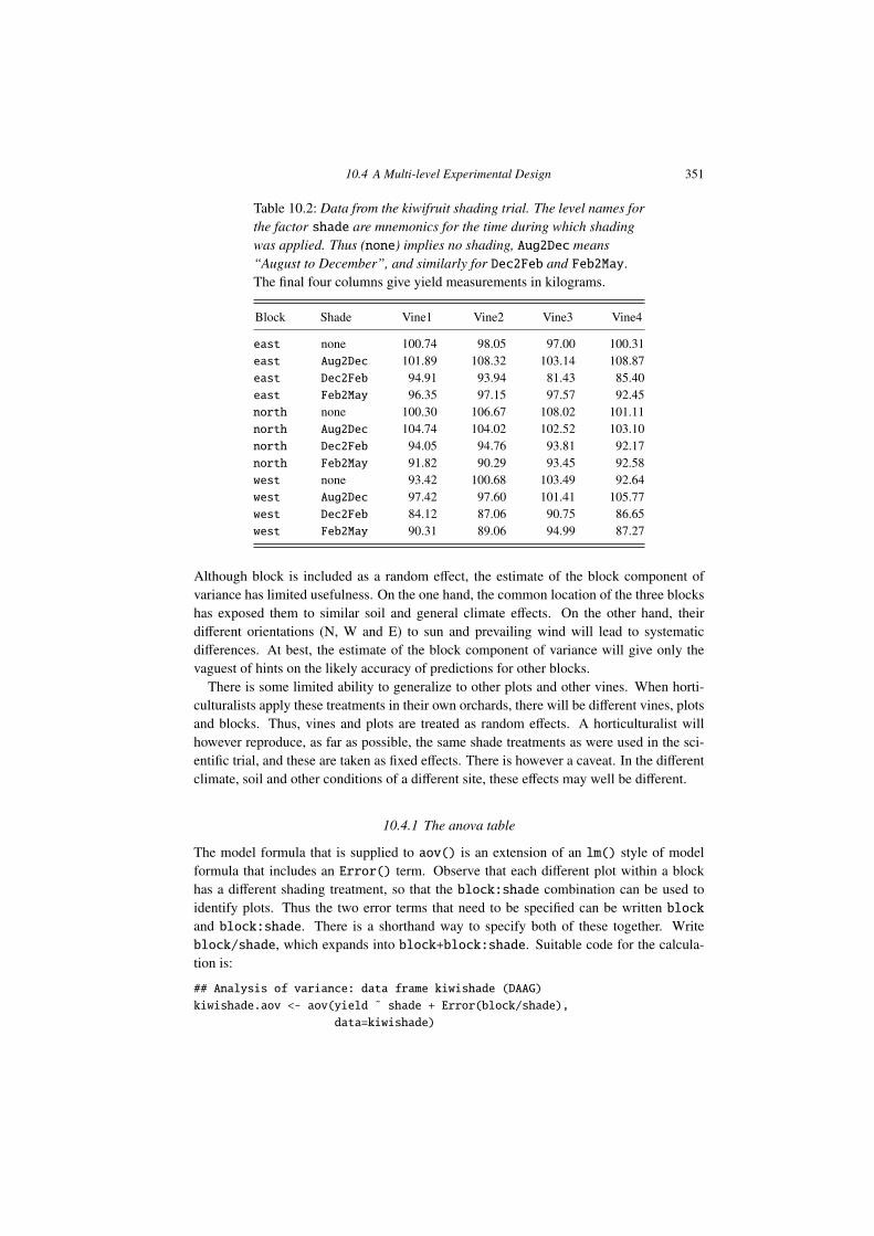
Table 10.2: Data from the kiwifruit shading trial. The level names forthe factor shade are mnemonics for the time during which shadingwas applied. Thus (none) implies no shading, Aug2Dec means“August to December”, and similarly for Dec2Feb and Feb2May.The final four columns give yield measurements in kilograms.
Block Shade Vine1 Vine2 Vine3 Vine4
east none 100.74 98.05 97.00 100.31east Aug2Dec 101.89 108.32 103.14 108.87east Dec2Feb 94.91 93.94 81.43 85.40east Feb2May 96.35 97.15 97.57 92.45north none 100.30 106.67 108.02 101.11north Aug2Dec 104.74 104.02 102.52 103.10north Dec2Feb 94.05 94.76 93.81 92.17north Feb2May 91.82 90.29 93.45 92.58west none 93.42 100.68 103.49 92.64west Aug2Dec 97.42 97.60 101.41 105.77west Dec2Feb 84.12 87.06 90.75 86.65west Feb2May 90.31 89.06 94.99 87.27
Although block is included as a random e↵ect, the estimate of the block component ofvariance has limited usefulness. On the one hand, the common location of the three blockshas exposed them to similar soil and general climate e↵ects. On the other hand, theirdi↵erent orientations (N, W and E) to sun and prevailing wind will lead to systematicdi↵erences. At best, the estimate of the block component of variance will give only thevaguest of hints on the likely accuracy of predictions for other blocks.
There is some limited ability to generalize to other plots and other vines. When horti-culturalists apply these treatments in their own orchards, there will be di↵erent vines, plotsand blocks. Thus, vines and plots are treated as random e↵ects. A horticulturalist willhowever reproduce, as far as possible, the same shade treatments as were used in the sci-entific trial, and these are taken as fixed e↵ects. There is however a caveat. In the di↵erentclimate, soil and other conditions of a di↵erent site, these e↵ects may well be di↵erent.
10.4.1 The anova table
The model formula that is supplied to aov() is an extension of an lm() style of modelformula that includes an Error() term. Observe that each di↵erent plot within a blockhas a di↵erent shading treatment, so that the block:shade combination can be used toidentify plots. Thus the two error terms that need to be specified can be written blockand block:shade. There is a shorthand way to specify both of these together. Writeblock/shade, which expands into block+block:shade. Suitable code for the calcula-tion is:
## Analysis of variance: data frame kiwishade (DAAG)
kiwishade.aov <- aov(yield ˜ shade + Error(block/shade),
data=kiwishade)
352 10. Multi-level Models, and Repeated Measures
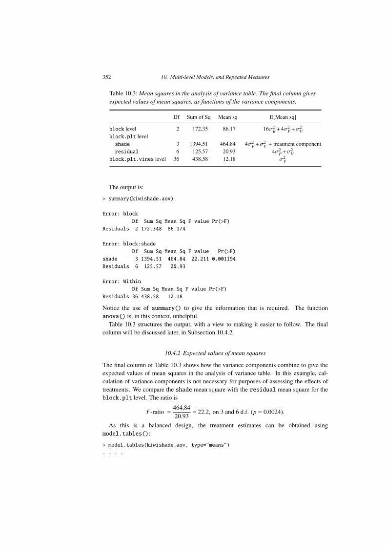
Table 10.3: Mean squares in the analysis of variance table. The final column givesexpected values of mean squares, as functions of the variance components.
Df Sum of Sq Mean sq E[Mean sq]
block level 2 172.35 86.17 16�2B+4�2
P +�2V
block.plt levelshade 3 1394.51 464.84 4�2
P +�2V + treatment component
residual 6 125.57 20.93 4�2P +�
2V
block.plt.vines level 36 438.58 12.18 �2V
The output is:
> summary(kiwishade.aov)
Error: block
Df Sum Sq Mean Sq F value Pr(>F)
Residuals 2 172.348 86.174
Error: block:shade
Df Sum Sq Mean Sq F value Pr(>F)
shade 3 1394.51 464.84 22.211 0.001194
Residuals 6 125.57 20.93
Error: Within
Df Sum Sq Mean Sq F value Pr(>F)
Residuals 36 438.58 12.18
Notice the use of summary() to give the information that is required. The functionanova() is, in this context, unhelpful.
Table 10.3 structures the output, with a view to making it easier to follow. The finalcolumn will be discussed later, in Subsection 10.4.2.
10.4.2 Expected values of mean squares
The final column of Table 10.3 shows how the variance components combine to give theexpected values of mean squares in the analysis of variance table. In this example, cal-culation of variance components is not necessary for purposes of assessing the e↵ects oftreatments. We compare the shade mean square with the residual mean square for theblock.plt level. The ratio is
F-ratio =464.8420.93
= 22.2, on 3 and 6 d.f. (p = 0.0024).
As this is a balanced design, the treatment estimates can be obtained usingmodel.tables():
> model.tables(kiwishade.aov, type="means")
. . . .
10.4 A Multi-level Experimental Design 353
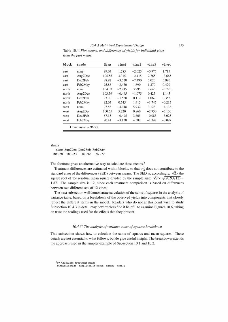
Table 10.4: Plot means, and di↵erences of yields for individual vinesfrom the plot mean.
block shade Mean vine1 vine2 vine3 vine4
east none 99.03 1.285 �2.025 �0.975 1.715east Aug2Dec 105.55 3.315 �2.415 2.765 �3.665east Dec2Feb 88.92 �3.520 �7.490 5.020 5.990east Feb2May 95.88 �3.430 1.690 1.270 0.470north none 104.03 �2.915 3.995 2.645 �3.725north Aug2Dec 103.59 �0.495 �1.075 0.425 1.145north Dec2Feb 93.70 �1.528 0.112 1.062 0.352north Feb2May 92.03 0.545 1.415 �1.745 �0.215west none 97.56 �4.918 5.932 3.123 �4.138west Aug2Dec 100.55 5.220 0.860 �2.950 �3.130west Dec2Feb 87.15 �0.495 3.605 �0.085 �3.025west Feb2May 90.41 �3.138 4.582 �1.347 �0.097
Grand mean = 96.53
shade
none Aug2Dec Dec2Feb Feb2May
100.20 103.23 89.92 92.77
The footnote gives an alternative way to calculate these means.5
Treatment di↵erences are estimated within blocks, so that �2B does not contribute to the
standard error of the di↵erences (SED) between means. The SED is, accordingly,p
2⇥ thesquare root of the residual mean square divided by the sample size:
p2⇥ p(20.93/12) =
1.87. The sample size is 12, since each treatment comparison is based on di↵erencesbetween two di↵erent sets of 12 vines.
The next subsection will demonstrate calculation of the sums of squares in the analysis ofvariance table, based on a breakdown of the observed yields into components that closelyreflect the di↵erent terms in the model. Readers who do not at this point wish to studySubsection 10.4.3 in detail may nevertheless find it helpful to examine Figures 10.6, takingon trust the scalings used for the e↵ects that they present.
10.4.3⇤ The analysis of variance sums of squares breakdown
This subsection shows how to calculate the sums of squares and mean squares. Thesedetails are not essential to what follows, but do give useful insight. The breakdown extendsthe approach used in the simpler example of Subsection 10.1 and 10.2.
5## Calculate treatment meanswith(kiwishade, sapply(split(yield, shade), mean))
354 10. Multi-level Models, and Repeated Measures
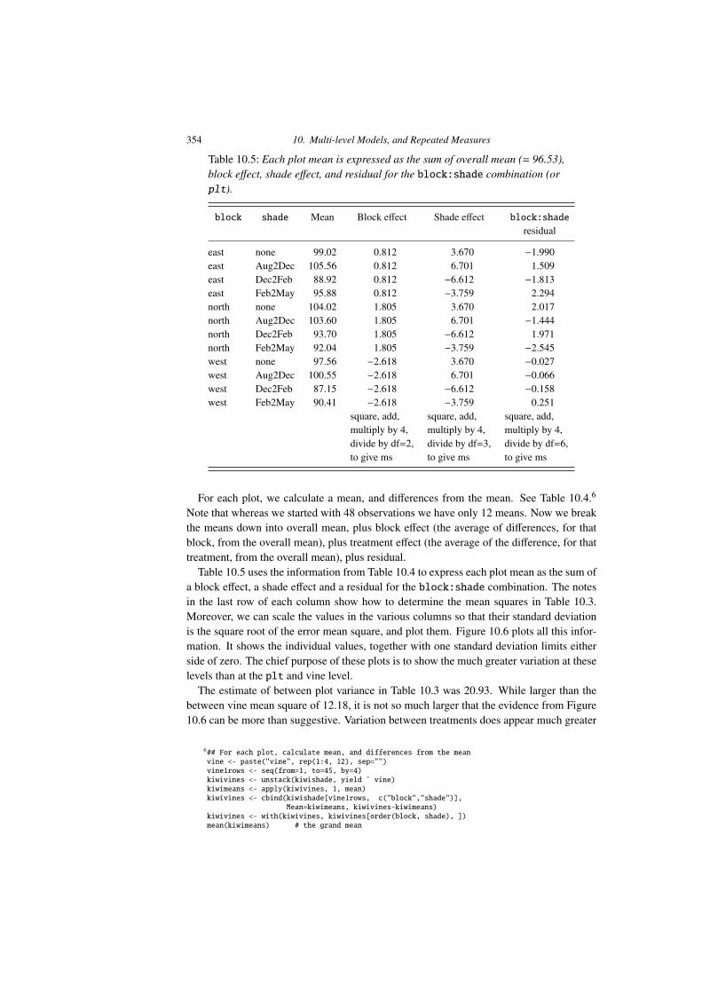
Table 10.5: Each plot mean is expressed as the sum of overall mean (= 96.53),block e↵ect, shade e↵ect, and residual for the block:shade combination (orplt).
block shade Mean Block e↵ect Shade e↵ect block:shade
residual
east none 99.02 0.812 3.670 �1.990east Aug2Dec 105.56 0.812 6.701 1.509east Dec2Feb 88.92 0.812 �6.612 �1.813east Feb2May 95.88 0.812 �3.759 2.294north none 104.02 1.805 3.670 2.017north Aug2Dec 103.60 1.805 6.701 �1.444north Dec2Feb 93.70 1.805 �6.612 1.971north Feb2May 92.04 1.805 �3.759 �2.545west none 97.56 �2.618 3.670 �0.027west Aug2Dec 100.55 �2.618 6.701 �0.066west Dec2Feb 87.15 �2.618 �6.612 �0.158west Feb2May 90.41 �2.618 �3.759 0.251
square, add, square, add, square, add,multiply by 4, multiply by 4, multiply by 4,divide by df=2, divide by df=3, divide by df=6,to give ms to give ms to give ms
For each plot, we calculate a mean, and di↵erences from the mean. See Table 10.4.6
Note that whereas we started with 48 observations we have only 12 means. Now we breakthe means down into overall mean, plus block e↵ect (the average of di↵erences, for thatblock, from the overall mean), plus treatment e↵ect (the average of the di↵erence, for thattreatment, from the overall mean), plus residual.
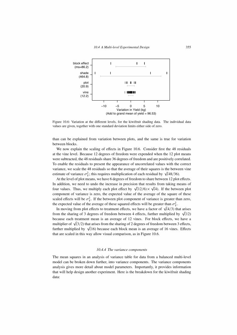
Table 10.5 uses the information from Table 10.4 to express each plot mean as the sum ofa block e↵ect, a shade e↵ect and a residual for the block:shade combination. The notesin the last row of each column show how to determine the mean squares in Table 10.3.Moreover, we can scale the values in the various columns so that their standard deviationis the square root of the error mean square, and plot them. Figure 10.6 plots all this infor-mation. It shows the individual values, together with one standard deviation limits eitherside of zero. The chief purpose of these plots is to show the much greater variation at theselevels than at the plt and vine level.
The estimate of between plot variance in Table 10.3 was 20.93. While larger than thebetween vine mean square of 12.18, it is not so much larger that the evidence from Figure10.6 can be more than suggestive. Variation between treatments does appear much greater
6## For each plot, calculate mean, and differences from the meanvine <- paste("vine", rep(1:4, 12), sep="")vine1rows <- seq(from=1, to=45, by=4)kiwivines <- unstack(kiwishade, yield ˜ vine)kiwimeans <- apply(kiwivines, 1, mean)kiwivines <- cbind(kiwishade[vine1rows, c("block","shade")],
Mean=kiwimeans, kiwivines-kiwimeans)kiwivines <- with(kiwivines, kiwivines[order(block, shade), ])mean(kiwimeans) # the grand mean
10.4 A Multi-level Experimental Design 355
−10 −5 0 5 10
| || | || | || | ||
||| |||||| |||
| || || || || || |
| |||| ||| ||| | |||| || || || || | ||| | ||||| ||||| || |||| |||
Variation in Yield (kg)(Add to grand mean of yield = 96.53)
vine(12.2)
plot(20.9)
shade(464.8)
block effect(ms=86.2)
Figure 10.6: Variation at the di↵erent levels, for the kiwifruit shading data. The individual datavalues are given, together with one standard deviation limits either side of zero.
than can be explained from variation between plots, and the same is true for variationbetween blocks.
We now explain the scaling of e↵ects in Figure 10.6. Consider first the 48 residualsat the vine level. Because 12 degrees of freedom were expended when the 12 plot meanswere subtracted, the 48 residuals share 36 degrees of freedom and are positively correlated.To enable the residuals to present the appearance of uncorrelated values with the correctvariance, we scale the 48 residuals so that the average of their squares is the between vineestimate of variance �2
V ; this requires multiplication of each residual byp
(48/36).At the level of plot means, we have 6 degrees of freedom to share between 12 plot e↵ects.
In addition, we need to undo the increase in precision that results from taking means offour values. Thus, we multiply each plot e↵ect by
p(12/6)⇥ p(4). If the between plot
component of variance is zero, the expected value of the average of the square of thesescaled e↵ects will be �2
V . If the between plot component of variance is greater than zero,the expected value of the average of these squared e↵ects will be greater than �2
V .In moving from plot e↵ects to treatment e↵ects, we have a factor of
p(4/3) that arises
from the sharing of 3 degrees of freedom between 4 e↵ects, further multiplied byp
(12)because each treatment mean is an average of 12 vines. For block e↵ects, we have amultiplier of
p(3/2) that arises from the sharing of 2 degrees of freedom between 3 e↵ects,
further multiplied byp
(16) because each block mean is an average of 16 vines. E↵ectsthat are scaled in this way allow visual comparison, as in Figure 10.6.
10.4.4 The variance components
The mean squares in an analysis of variance table for data from a balanced multi-levelmodel can be broken down further, into variance components. The variance componentsanalysis gives more detail about model parameters. Importantly, it provides informationthat will help design another experiment. Here is the breakdown for the kiwifruit shadingdata:
356 10. Multi-level Models, and Repeated Measures
• Variation between vines in a plot is made up of one source of variation only. Denotethis variance by �2
V .• Variation between vines in di↵erent plots is partly a result of variation between vines,
and partly a result of additional variation between plots. In fact, if �2P is the (additional)
component of the variation that is due to variation between plots, the expected meansquare equals
4�2P+�
2V .
(NB: the 4 comes from 4 vines per plot.)• Variation between treatments is
4�2P+�
2V +T
where T (> 0) is due to variation between treatments.• Variation between vines in di↵erent blocks is partly a result of variation between vines,
partly a result of additional variation between plots, and partly a result of additionalvariation between blocks. If �2
B is the (additional) component of variation that is due todi↵erences between blocks, the expected value of the mean square is
16�2B+4�2
P+�2V
(16 vines per block; 4 vines per plot).
We do not need estimates of the variance components in order to do the analysis ofvariance. The variance components are helpful for designing another experiment. Wecalculate the estimates thus:
b�2V = 12.18,
4b�2P+b�2
V = 20.93, i.e. 4b�2P+12.18 = 20.93.
This gives the estimate b�2P = 2.19. We can also estimate b�2
B = 4.08.We are now in a position to work out how much the precision would change if we had 8
(or, say, 10) vines per plot. With n vines per plot, the variance of the plot mean is
(nb�2P+b�2
V )/n = b�2P+b�2
V/n = 2.19+12.18/n.
We could also ask how much of the variance, for an individual vine, is explained by vineto vine di↵erences. This depends on how much we stretch the other sources of variation.If the comparison is with vines that may be in di↵erent plots, the proportion is 12.18/(12.18+ 2.19). If we are talking about di↵erent blocks, the proportion is 12.18/(12.18+2.19+4.08).
10.4.5 The mixed model analysis
For a mixed model analysis, we specify that treatment (shade) is a fixed e↵ect, that blockand plot are random e↵ects, and that plot is nested in block. The software works out foritself that the remaining part of the variation is associated with di↵erences between vines.
For using lmer(), the command is
10.4 A Multi-level Experimental Design 357
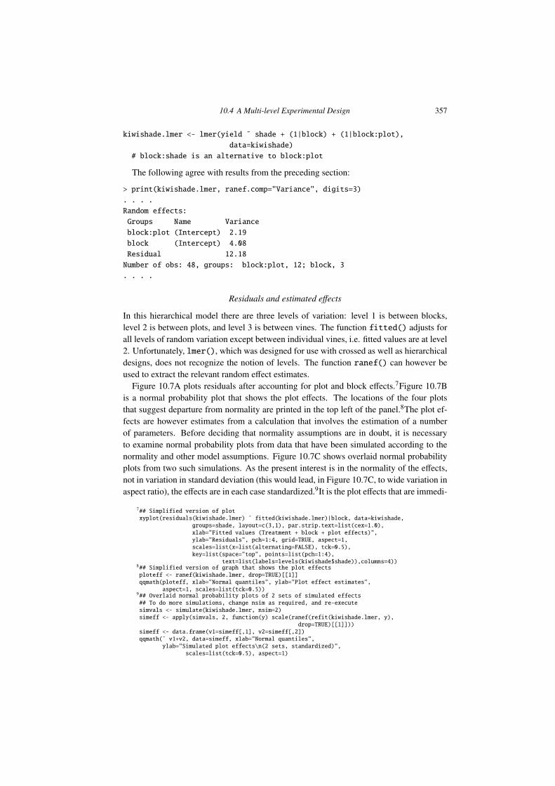
kiwishade.lmer <- lmer(yield ˜ shade + (1|block) + (1|block:plot),
data=kiwishade)
# block:shade is an alternative to block:plot
The following agree with results from the preceding section:
> print(kiwishade.lmer, ranef.comp="Variance", digits=3)
. . . .
Random effects:
Groups Name Variance
block:plot (Intercept) 2.19
block (Intercept) 4.08
Residual 12.18
Number of obs: 48, groups: block:plot, 12; block, 3
. . . .
Residuals and estimated e↵ects
In this hierarchical model there are three levels of variation: level 1 is between blocks,level 2 is between plots, and level 3 is between vines. The function fitted() adjusts forall levels of random variation except between individual vines, i.e. fitted values are at level2. Unfortunately, lmer(), which was designed for use with crossed as well as hierarchicaldesigns, does not recognize the notion of levels. The function ranef() can however beused to extract the relevant random e↵ect estimates.
Figure 10.7A plots residuals after accounting for plot and block e↵ects.7Figure 10.7Bis a normal probability plot that shows the plot e↵ects. The locations of the four plotsthat suggest departure from normality are printed in the top left of the panel.8The plot ef-fects are however estimates from a calculation that involves the estimation of a numberof parameters. Before deciding that normality assumptions are in doubt, it is necessaryto examine normal probability plots from data that have been simulated according to thenormality and other model assumptions. Figure 10.7C shows overlaid normal probabilityplots from two such simulations. As the present interest is in the normality of the e↵ects,not in variation in standard deviation (this would lead, in Figure 10.7C, to wide variation inaspect ratio), the e↵ects are in each case standardized.9It is the plot e↵ects that are immedi-
7## Simplified version of plotxyplot(residuals(kiwishade.lmer) ˜ fitted(kiwishade.lmer)|block, data=kiwishade,
groups=shade, layout=c(3,1), par.strip.text=list(cex=1.0),xlab="Fitted values (Treatment + block + plot effects)",ylab="Residuals", pch=1:4, grid=TRUE, aspect=1,scales=list(x=list(alternating=FALSE), tck=0.5),key=list(space="top", points=list(pch=1:4),
text=list(labels=levels(kiwishade$shade)),columns=4))8## Simplified version of graph that shows the plot effectsploteff <- ranef(kiwishade.lmer, drop=TRUE)[[1]]qqmath(ploteff, xlab="Normal quantiles", ylab="Plot effect estimates",
aspect=1, scales=list(tck=0.5))9## Overlaid normal probability plots of 2 sets of simulated effects## To do more simulations, change nsim as required, and re-executesimvals <- simulate(kiwishade.lmer, nsim=2)simeff <- apply(simvals, 2, function(y) scale(ranef(refit(kiwishade.lmer, y),
drop=TRUE)[[1]]))simeff <- data.frame(v1=simeff[,1], v2=simeff[,2])qqmath(˜ v1+v2, data=simeff, xlab="Normal quantiles",
ylab="Simulated plot effects\n(2 sets, standardized)",scales=list(tck=0.5), aspect=1)
358 10. Multi-level Models, and Repeated Measures
Fitted values (Treatment + block + plot effects)
Res
idua
ls
−5
0
5
90 95 100 105
●
●●
●
east
90 95 100 105
●
●
●
●
north
90 95 100 105
●
●
●
●
west
● none Aug2Dec Dec2Feb Feb2MayA
Normal quantiles
Plot
effe
ct e
stim
ates
−0.5
0.0
0.5
1.0
−1 0 1
●●
●
●● ● ●
●
●
● ● ●Feb2May:eastnone:northDec2Feb:northAug2Dec:east
B
Normal quantiles
Sim
ulat
ed p
lot e
ffect
s(2
set
s, s
tand
ardi
zed)
−2
−1
0
1
−1 0 1
●
●●
●
●● ●
● ●
●●
●
C
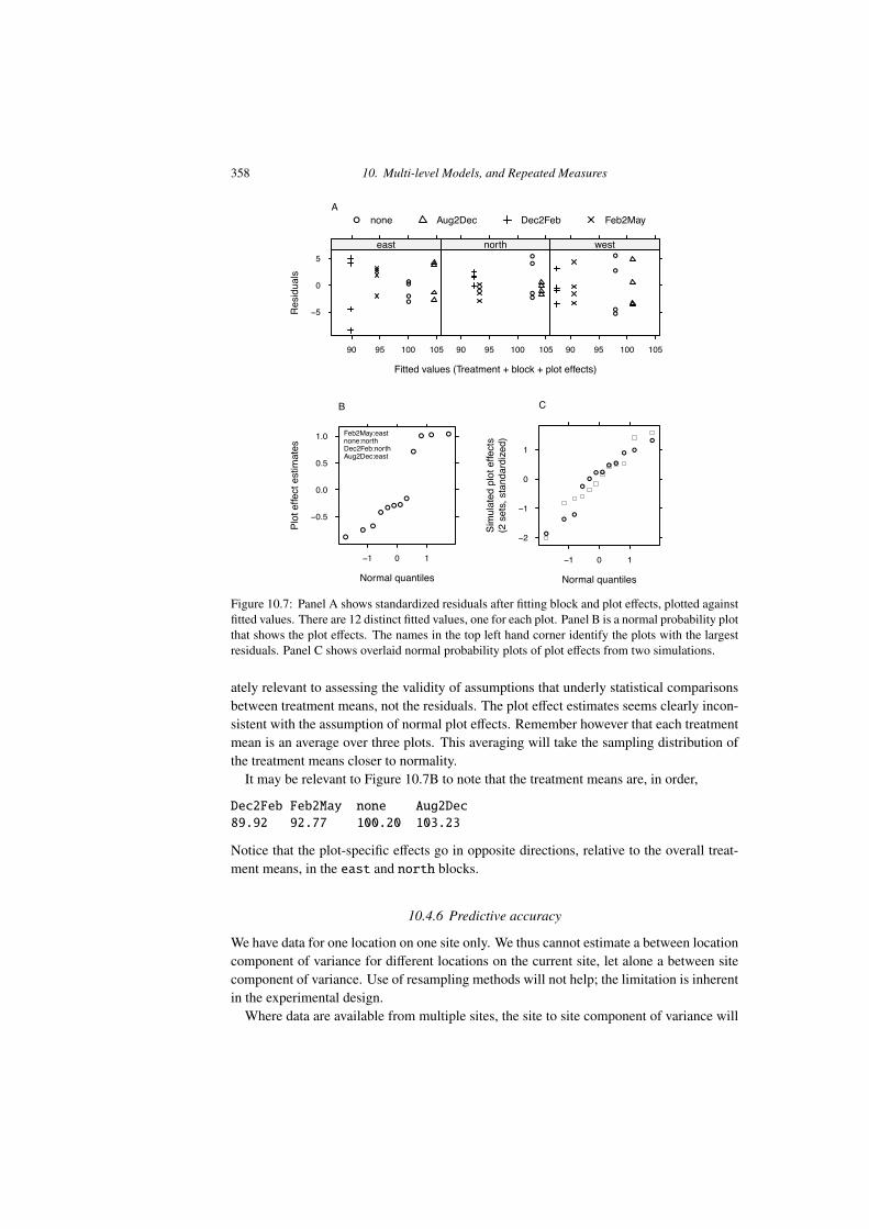
Figure 10.7: Panel A shows standardized residuals after fitting block and plot e↵ects, plotted againstfitted values. There are 12 distinct fitted values, one for each plot. Panel B is a normal probability plotthat shows the plot e↵ects. The names in the top left hand corner identify the plots with the largestresiduals. Panel C shows overlaid normal probability plots of plot e↵ects from two simulations.
ately relevant to assessing the validity of assumptions that underly statistical comparisonsbetween treatment means, not the residuals. The plot e↵ect estimates seems clearly incon-sistent with the assumption of normal plot e↵ects. Remember however that each treatmentmean is an average over three plots. This averaging will take the sampling distribution ofthe treatment means closer to normality.
It may be relevant to Figure 10.7B to note that the treatment means are, in order,
Dec2Feb Feb2May none Aug2Dec89.92 92.77 100.20 103.23
Notice that the plot-specific e↵ects go in opposite directions, relative to the overall treat-ment means, in the east and north blocks.
10.4.6 Predictive accuracy
We have data for one location on one site only. We thus cannot estimate a between locationcomponent of variance for di↵erent locations on the current site, let alone a between sitecomponent of variance. Use of resampling methods will not help; the limitation is inherentin the experimental design.
Where data are available from multiple sites, the site to site component of variance will
10.5 Within and Between Subject E↵ects 359
almost inevitably be greater than zero. Given adequate data, the estimate of this componentof variance will then also be greater than zero, even in the presence of explanatory variableadjustments that attempt to adjust for di↵erences in rainfall, temperature, soil type, etc.(Treatment di↵erences are often, but by no means inevitably, more nearly consistent acrosssites than are the treatment means themselves.)
Where two (or more) experimenters use di↵erent sites, di↵erences in results are to beexpected. Such di↵erent results have sometimes led to acriminious exchanges, with eachconvinced that there are flaws in the other’s experimental work. Rather, assuming that bothexperiments were conducted with proper care, the implication is that both sets of resultsshould be incorporated into an analysis that accounts for site to site variation. Better still,plan the experiment from the beginning as a multi-site experiment!
10.5 Within and Between Subject E↵ects
The data frame tinting is from an experiment that aimed to model the e↵ects of thetinting of car windows on visual performance. (For more information, see Burns et al.,1999.) Interest is focused on e↵ects on side window vision, and hence on visual recognitiontasks that would be performed when looking through side windows.
The variables are csoa (critical stimulus onset asynchrony, i.e., the time in millisecondsrequired to recognize an alphanumeric target), it (inspection time, i.e., the time requiredfor a simple discrimination task) and age, while tint (three levels) and target (twolevels) are ordered factors. The variable sex is coded f for females and m for males, whilethe variable agegp is coded Younger for young people (all in their 20s) and Older forolder participants (all in their 70s).
Data were collected in two sessions, with half the individuals undertaking the csoa taskin the first session and the it task in the second session, and the other half doing these twotypes of task in the reverse order. Within each session, the order of presentation of the twolevels of target contrast was balanced over participants. For each level of target contrast thelevels of tint were in the order no (100% VLT = visible light transmittance), lo (81.3%VLT = visible light transmittance) and hi (35% VLT = visible light transmittance). Eachparticipant repeated the combination of high contrast with no tinting (100% VLT) at theend of the session. Comparison with the same task from earlier in the session thus allowsa check on any change in performance through the session.
We have two levels of variation – within individuals (who were each tested on eachcombination of tint and target), and between individuals. Thus we need to specify id(identifying the individual) as a random e↵ect. Plots of the data make it clear that, to havevariances that are approximately homogeneous, we need to work with log(csoa) andlog(it). Here, we describe the analysis for log(it).
Model fitting criteria
The function lmer() allows use of one of two criteria: restricted (or residual) maximumlikelihood (REML), which is the default, and maximum likelihood (ML). The parameterestimates from the REML method are generally preferred to those from ML, as more nearlyunbiased. Comparison of models using anova() relies on maximum likelihood theory, and
360 10. Multi-level Models, and Repeated Measures
the models should be fitted using ML.
10.5.1 Model selection
A good principle is to limit initial comparisons between models to several alternative mod-els within a hierarchy of increasing complexity. For example, consider main e↵ects only,main e↵ects plus all first order interactions, main e↵ects plus all first and second orderinteractions, as far on up this hierarchy as seems reasonable. This makes for conceptualclarity, and simplifies inference. (Where a model has been selected from a large number ofcandidate models, selection e↵ects come into play, and inference must account for this.)
Here, three models will be considered:
1. All possible interactions (this is likely to be more complex than is needed):## Change initial letters of levels of tinting$agegp to upper case
library(R.utils)
levels(tinting$agegp) <- capitalize(levels(tinting$agegp))
## Fit all interactions: data frame tinting (DAAG)
it3.lmer <- lmer(log(it) ˜ tint*target*agegp*sex + (1 | id),
data=tinting, REML=FALSE)
2. All two-factor interactions (this is a reasonable guess; two-factor interactions may beall we need):it2.lmer <- lmer(log(it) ˜ (tint+target+agegp+sex)ˆ2 + (1 | id),
data=tinting, REML=FALSE)
3. Main e↵ects only (this is a very simple model):it1.lmer <- lmer(log(it)˜(tint+target+agegp+sex) + (1 | id),
data=tinting, REML=FALSE)
The use of REML=FALSE; is advisable for the anova() (likelihood ratio) comparison thatnow follows:
> anova(it1.lmer, it2.lmer, it3.lmer)
Data: tinting
Models:
it1.lmer: log(it) ˜ (tint + target + agegp + sex) + (1 | id)
it2.lmer: log(it) ˜ (tint + target + agegp + sex)ˆ2 + (1 | id)
it3.lmer: log(it) ˜ tint * target * agegp * sex + (1 | id)
Df AIC BIC logLik Chisq Chi Df Pr(>Chisq)
it1.lmer 7 -0.9 21.6 7.4
it2.lmer 16 -5.7 45.5 18.9 22.88 9 0.0065
it3.lmer 25 6.1 86.2 21.9 6.11 9 0.7288
Notice that Df is now used for degrees of freedom, where DF was used in connection withsummary.aov(). earlier.
The p-value for comparing model 1 with model 2 is 0.73, while that for comparingmodel 2 with model 3 is 0.0065. This suggests that the model that limits attention to two-factor interactions is adequate. (Note also that the AIC statistic favors model 2. The BICstatistic, which is an alternative to AIC, favors the model that has main e↵ects only.
Hastie et al. (2009, p. 235) suggest, albeit in reference to models with i.i.d. errors, thatBIC’s penalty for model complexity can be unduly severe when the number of residualdegrees of freedom is small. (Note also that the di↵erent standard errors are based on vari-
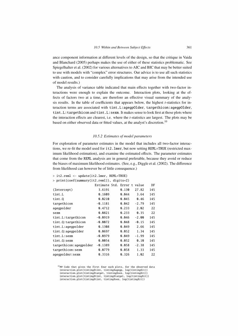
10.5 Within and Between Subject E↵ects 361
ance component information at di↵erent levels of the design, so that the critique in Vaidaand Blanchard (2005) perhaps makes the use of either of these statistics problematic. SeeSpiegelhalter et al. (2002) for various alternatives to AIC and BIC that may be better suitedto use with models with “complex” error structures. Our advice is to use all such statisticswith caution, and to consider carefully implications that may arise from the intended useof model results.)
The analysis of variance table indicated that main e↵ects together with two-factor in-teractions were enough to explain the outcome. Interaction plots, looking at the ef-fects of factors two at a time, are therefore an e↵ective visual summary of the analy-sis results. In the table of coe�cients that appears below, the highest t-statistics for in-teraction terms are associated with tint.L:agegpOlder, targethicon:agegpOlder,tint.L:targethicon and tint.L:sexm. It makes sense to look first at those plots wherethe interaction e↵ects are clearest, i.e. where the t-statistics are largest. The plots may bebased on either observed data or fitted values, at the analyst’s discretion.10
10.5.2 Estimates of model parameters
For exploration of parameter estimates in the model that includes all two-factor interac-tions, we re-fit the model used for it2.lmer, but now setting REML=TRUE (restricted max-imum likelihood estimation), and examine the estimated e↵ects. The parameter estimatesthat come from the REML analysis are in general preferable, because they avoid or reducethe biases of maximum likelihood estimates. (See, e.g., Diggle et al. (2002). The di↵erencefrom likelihood can however be of little consequence.)
> it2.reml <- update(it2.lmer, REML=TRUE)
> print(coef(summary(it2.reml)), digits=2)
Estimate Std. Error t value DF
(Intercept) 3.6191 0.130 27.82 145
tint.L 0.1609 0.044 3.64 145
tint.Q 0.0210 0.045 0.46 145
targethicon -0.1181 0.042 -2.79 145
agegpolder 0.4712 0.233 2.02 22
sexm 0.0821 0.233 0.35 22
tint.L:targethicon -0.0919 0.046 -2.00 145
tint.Q:targethicon -0.0072 0.048 -0.15 145
tint.L:agegpolder 0.1308 0.049 2.66 145
tint.Q:agegpolder 0.0697 0.052 1.34 145
tint.L:sexm -0.0979 0.049 -1.99 145
tint.Q:sexm 0.0054 0.052 0.10 145
targethicon:agegpolder -0.1389 0.058 -2.38 145
targethicon:sexm 0.0779 0.058 1.33 145
agegpolder:sexm 0.3316 0.326 1.02 22
10## Code that gives the first four such plots, for the observed datainteraction.plot(tinting$tint, tinting$agegp, log(tinting$it))interaction.plot(tinting$target, tinting$sex, log(tinting$it))interaction.plot(tinting$tint, tinting$target, log(tinting$it))interaction.plot(tinting$tint, tinting$sex, log(tinting$it))
362 10. Multi-level Models, and Repeated Measures
> # NB: The final column, giving degrees of freedom, is not in the
> # summary output. It is our addition.
Because tint is an ordered factor with three levels, its e↵ect is split up into two parts.The first, which always carries a .L (linear) label, checks if there is a linear change acrosslevels. The second part is labeled .Q (quadratic), and as tint has only three levels, ac-counts for all the remaining sum of squares that is due to tint. A comparable partitioningof the e↵ect of tint carries across to interaction terms also.
The t-statistics for interactions involving tint.Q are 0.46, -0.15, 1.34 and 1.10. Theoutput can be simplified by omitting these interactions.
None of the main e↵ects and interactions involving agegp and sex are significant atthe conventional 5% level, though agegp comes close. On the other hand, the interactionterms (tint.L:agegpOlder, targethicon:agegpOlder, tint.L:targethicon andtint.L:sexm) that are statistically significant stand out much less clearly in Figures 2.12Aand 2.12B.
This may seem inconsistent with Figures 2.12A and 2.12B, where it is the older maleswho seem to have the longer times. To resolve this apparent inconsistency, observe that
• Comparisons that relate to agegp and sex are made relative to variation between in-dividuals. Standard errors for such comparisons, in the output, are in the range 0.23- 0.32, in each case with 22 degrees of freedom. (There are 9 younger and 4 olderfemales, against 4 younger and 9 older males.11 )
• Comparisons between levels of tint or target are made several times for each of the26 individuals, and are relatively consistent from one individual to another. Standarderrors for these comparisons are small – in the range 0.042 - 0.058.
Statistical variation cannot be convincingly ruled out as the explanation for the e↵ectsthat stand out most strongly in the graphs. The graphs are not designed to highlight theconsistency with which individuals respond to di↵erences between levels of tinting andtarget contrast.
10.6 A Generalized Linear Mixed Model
Consider again the moths data of Subsection 8.4.2. The analysis in Subsection 8.4.2 as-sumed a quasipoisson error, which uses a constant multiplier for the Poisson variance. Itmay be better to assume a random between transects error that is additive on the scale ofthe linear predictor. The model incorporates a term that allows for normally distributedrandom variation, additional to the poisson variation at each observation. Technically, thisis an example of the use of “observation level random e↵ects”.
The attempt to fit a model that uses the default log link generates (lme4 1.1-7), if datafor the habitat Bank is included, a warning that the model is nearly unidentifiable. Thisproblem is avoided if a square root link is used.
The code is:moths$transect <- 1:41 # Each row is from a different transect
moths$habitat <- relevel(moths$habitat, ref="Lowerside")
11subs <- with(tinting, match(unique(id), id)); with(tinting, table(sex[subs], agegp[subs]))
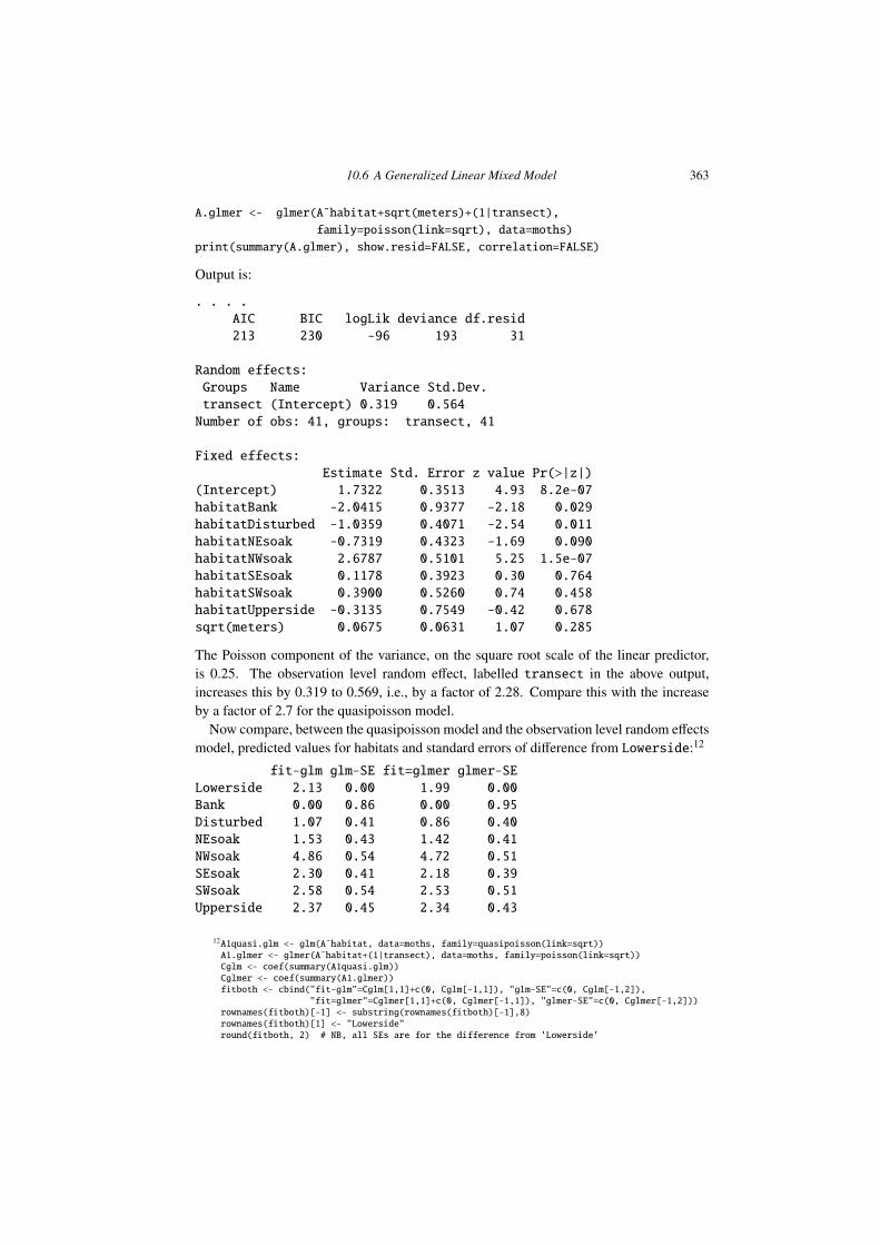
10.6 A Generalized Linear Mixed Model 363
A.glmer <- glmer(A˜habitat+sqrt(meters)+(1|transect),
family=poisson(link=sqrt), data=moths)
print(summary(A.glmer), show.resid=FALSE, correlation=FALSE)
Output is:
. . . .AIC BIC logLik deviance df.resid213 230 -96 193 31
Random effects:Groups Name Variance Std.Dev.transect (Intercept) 0.319 0.564Number of obs: 41, groups: transect, 41
Fixed effects:Estimate Std. Error z value Pr(>|z|)
(Intercept) 1.7322 0.3513 4.93 8.2e-07habitatBank -2.0415 0.9377 -2.18 0.029habitatDisturbed -1.0359 0.4071 -2.54 0.011habitatNEsoak -0.7319 0.4323 -1.69 0.090habitatNWsoak 2.6787 0.5101 5.25 1.5e-07habitatSEsoak 0.1178 0.3923 0.30 0.764habitatSWsoak 0.3900 0.5260 0.74 0.458habitatUpperside -0.3135 0.7549 -0.42 0.678sqrt(meters) 0.0675 0.0631 1.07 0.285
The Poisson component of the variance, on the square root scale of the linear predictor,is 0.25. The observation level random e↵ect, labelled transect in the above output,increases this by 0.319 to 0.569, i.e., by a factor of 2.28. Compare this with the increaseby a factor of 2.7 for the quasipoisson model.
Now compare, between the quasipoisson model and the observation level random e↵ectsmodel, predicted values for habitats and standard errors of di↵erence from Lowerside:12
fit-glm glm-SE fit=glmer glmer-SELowerside 2.13 0.00 1.99 0.00Bank 0.00 0.86 0.00 0.95Disturbed 1.07 0.41 0.86 0.40NEsoak 1.53 0.43 1.42 0.41NWsoak 4.86 0.54 4.72 0.51SEsoak 2.30 0.41 2.18 0.39SWsoak 2.58 0.54 2.53 0.51Upperside 2.37 0.45 2.34 0.43
12A1quasi.glm <- glm(A˜habitat, data=moths, family=quasipoisson(link=sqrt))A1.glmer <- glmer(A˜habitat+(1|transect), data=moths, family=poisson(link=sqrt))Cglm <- coef(summary(A1quasi.glm))Cglmer <- coef(summary(A1.glmer))fitboth <- cbind("fit-glm"=Cglm[1,1]+c(0, Cglm[-1,1]), "glm-SE"=c(0, Cglm[-1,2]),
"fit=glmer"=Cglmer[1,1]+c(0, Cglmer[-1,1]), "glmer-SE"=c(0, Cglmer[-1,2]))rownames(fitboth)[-1] <- substring(rownames(fitboth)[-1],8)rownames(fitboth)[1] <- "Lowerside"round(fitboth, 2) # NB, all SEs are for the difference from 'Lowerside'
364 10. Multi-level Models, and Repeated Measures
Observe that the standard errors for comparisons with Lowerside are similar for thetwo models. The fitted values in the the observation level random e↵ects model are pulledin towards zero, relative to the quasipoisson model.
It is left as an exercise for the reader to compare the plots of residuals versus fitted valuesbetween the two models.
Mixed models with a binomial error and logit link
On a logit scale, the binomial contribution to the error increases as the expected valuemoves away from 0.5. (One the scale of the response, however, error decreases as the ex-pected value moves away from 0.5). Thus, relative to a quasibinomial model, the SED willbe reduced for more extreme comparisons, and increased for less extreme comparisons.
10.7 Repeated Measures in Time
Whenever we make repeated measurements on a treatment unit we are, technically, work-ing with repeated measures. In this sense, both the kiwifruit shading data and the windowtinting data sets were examples of repeated measures data sets. Here, our interest is in gen-eralizing the multi-level modeling approach to handle models for longitudinal data, i.e.,data where the measurements were repeated at di↵erent times.
In the kiwifruit shading experiment, we gathered data from all vines in a plot at the onetime. In principle, we might have taken data from di↵erent vines at di↵erent points in time.For each plot, there would then be data at each of four time points.
There is a close link between a wide class of repeated measures models and time seriesmodels. In the time series context, there is usually just one realization of the series, whichmay however be observed at a large number of time points. In the repeated measurescontext, there may be a large number of realizations of a series that is typically quite short.
Perhaps the simplest case is where there is no apparent trend with time. Thus considerdata from a clinical trial of a drug (progabide) used to control epileptic fits. (For an anal-ysis of data from the study to which this example refers, see Thall and Vail, 1990.) Theanalysis assumes that patients were randomly assigned to the two treatments – placebo andprogabide. After an eight-week run-in period, data were collected, both for the placebogroup and for the progabide group, in each of four successive two-week periods. Theoutcome variable was the number of epileptic fits over that time.
One way to do the analysis is to work with the total number of fits over the four weeks,perhaps adjusted by subtracting the baseline value. It is possible that we might obtain extrasensitivity by taking account of the correlation structure between the four sets of fortnightlyresults, taking a weighted sum rather than a mean.
Where there is a trend with time, working with a mean over all times will not usuallymake sense. Any or all of the following can occur, both for the overall pattern of changeand for the pattern of di↵erence between one profile and another.
1. There is no trend with time.2. The pattern with time may follow a simple form, e.g., a line or a quadratic curve.3. A general form of smooth curve, e.g., a curve fitted using splines, may be required to
10.7 Repeated Measures in Time 365
account for the pattern of change with time.
The theory of repeated measures modeling
For the moment, profiles (or subjects) are assumed independent. The analysis must allowfor dependencies between the results of any one subject at di↵erent times. For a balanceddesign, we will assume n subjects (i = 1,2, . . . ,n) and p times ( j = 1,2, . . . , p), though per-haps with missing responses (gaps) for some subjects at some times. The plot of responseversus time for any one subject is that subject’s profile.
A key idea is that there are (at least) two levels of variability – between subjects andwithin subjects. In addition, there is measurement error.
Repeating the same measurement on the same subject at the same time will not giveexactly the same result. The between subjects component of variation is never observableseparately from sources of variation that operate “within subjects”. In any data that we col-lect, measurements are always a↵ected by “within subjects” variability, plus measurementerror. Thus the simplest model that is commonly used has a between subjects variancecomponent denoted by ⌫2, while there is a within subjects variance at any individual timepoint that is denoted by �2. The measurement error may be bundled in as part of �2. Thevariance of the response for one subject at a particular time point is ⌫2+�2.
In the special case just considered, the variance of the di↵erence between two time pointsfor one subject is 2�2. Comparisons “within subjects” are more accurate than comparisons“between subjects”.
*Correlation structure
The time dependence of the data has implications for the correlation structure. The simplemodel just described takes no account of this structure. Often, the separation of points intime is reflected in a correlation between time points that decreases as the time separationincreases. The variance for di↵erences between times may increase as points move furtherapart in time.
We have seen that correlation structure is also a key issue in time series analysis. Alimitation, relative to repeated measures, is that in time series analysis the structure musttypically be estimated from just one series, by assuming that the series is in some sensepart of a repeating pattern. In repeated measures there may be many realizations, allowinga relatively accurate estimate of the correlation structure. By contrast with time series,the shortness of the series has no e↵ect on our ability to estimate the correlation structure.Multiple realizations are preferable to a single long series.
While we are typically better placed than in time series analysis to estimate the corre-lation structure there is, for most of the inferences that we commonly wish to make, lessneed to know the correlation structure. Typically our interest is in the consistency of pat-terns between individuals. For example we may want to know: “Do patients on treatmentA improve at a greater rate than patients on treatment B?”
There is a broad distinction between approaches that model the profiles, and approachesthat focus more directly on modeling the correlation structure. Direct modeling of theprofiles leads to random coe�cient models, which allow each individual to follow theirown profile. Variation between profiles may largely account for the sequential correlationstructure. Direct modeling of the correlation is most e↵ective when there are no evidentsystematic di↵erences between profiles.
366 10. Multi-level Models, and Repeated Measures
For further discussion of repeated measures modeling, see Diggle et al. (2002); Pinheiroand Bates (2000). The Pinheiro and Bates book is based around the S-PLUS version of thenlme package.
Di↵erent approaches to repeated measures analysis
Traditionally, repeated measures models have been analyzed in many di↵erent ways. Hereis a summary of methods that have been used:
• A simple way to analyze repeated measures data is to form one or more summarystatistics for each subject, and then use these summary statistics for further analysis.
• When the variance is the same at all times and the correlation between results is thesame for all pairs of times, data can in principle be analyzed using an analysis of vari-ance model. This allows for two components of variance, (1) between subjects and (2)between times. An implication of this model is that the variance of the di↵erence is thesame for all pairs of time points, an assumption that is, in general, unrealistic.
• Various adjustments adapt the analysis of variance approach to allow for the possibilitythat the variance of time di↵erences are not all equal. These should be avoided nowthat there are good alternatives to the analysis of variance approach.
• Multivariate comparisons accommodate all possible patterns of correlations betweentime points. This approach accommodates the time series structure, but does not takeadvantage of it to find an economical parameterization of the correlation structure.
• Repeated measures models aim to reflect the sequential structure, in the fixed e↵ects, inthe random e↵ects, and in the correlation structure. They do this in two ways: by mod-eling the overall pattern of di↵erence between di↵erent profiles, and by direct modelingof the correlation structure. This modeling approach often allows insights that are hardto gain from approaches that ignore or do not take advantage of the sequential structure.
10.7.1 Example – random variation between profiles
The data frame humanpower1 has data from investigations (Bussolari, 1987; Nadel andBussolari, 1988) designed to assess the feasibility of a proposed 119 kilometer humanpowered flight from the island of Crete – in the initial phase of the Daedalus project. Afteran initial 5-minute warm-up period and 5-minute recovery period, the power requirementsfrom the athletes were increased, at two-minute intervals, in steps of around 30 watts.Figure 10.8 gives a visual summary of the data.13
We leave it as an exercise to verify, using a fixed e↵ects analysis such as was describedin Section 7.3, that separate lines are required for the di↵erent athletes, and that there is no
13## Plot points and fitted lines (panel A)library(lattice)xyplot(o2 ˜ wattsPerKg, groups=id, data=humanpower1,
panel=function(x,y,subscripts,groups,...){yhat <- fitted(lm(y ˜ groups*x))panel.superpose(x, y, subscripts, groups, pch=1:5)panel.superpose(x, yhat, subscripts, groups, type="l")
},xlab="Watts per kilogram",ylab=expression("Oxygen intake ("*ml.minˆ{-1}*.kgˆ{-1}*")"))
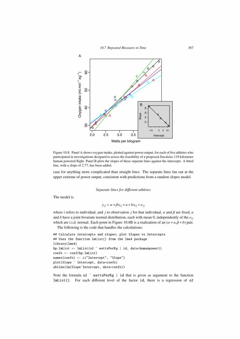
10.7 Repeated Measures in Time 367
●
●
● ●
●
●●
●
2.0 2.5 3.0 3.5 4.0 4.5
3040
5060
Watts per kilogram
Oxy
gen
inta
ke (m
l.min−−1
.kg−−
1 )
A
−10 0 5 10
1214
1618
Intercept
Slop
e
−10 0 5 10
1214
1618
●
B
InterceptSl
ope
Figure 10.8: Panel A shows oxygen intake, plotted against power output, for each of five athletes whoparticipated in investigations designed to assess the feasibility of a proposed Daedalus 119 kilometerhuman powered flight. Panel B plots the slopes of these separate lines against the intercepts. A fittedline, with a slope of 2.77, has been added.
case for anything more complicated than straight lines. The separate lines fan out at theupper extreme of power output, consistent with predictions from a random slopes model.
Separate lines for di↵erent athletes
The model is
yi j = ↵+�xi j+a+bxi j+ ei j
where i refers to individual, and j to observation j for that individual, ↵ and � are fixed, aand b have a joint bivariate normal distribution, each with mean 0, independently of the ei jwhich are i.i.d. normal. Each point in Figure 10.8B is a realization of an (↵+a,�+b) pair.
The following is the code that handles the calculations:
## Calculate intercepts and slopes; plot Slopes vs Intercepts
## Uses the function lmList() from the lme4 package
library(lme4)
hp.lmList <- lmList(o2 ˜ wattsPerKg | id, data=humanpower1)
coefs <- coef(hp.lmList)
names(coefs) <- c("Intercept", "Slope")
plot(Slope ˜ Intercept, data=coefs)
abline(lm(Slope˜Intercept, data=coefs))
Note the formula o2 ˜ wattsPerKg | id that is given as argument to the functionlmList(). For each di↵erent level of the factor id, there is a regression of o2
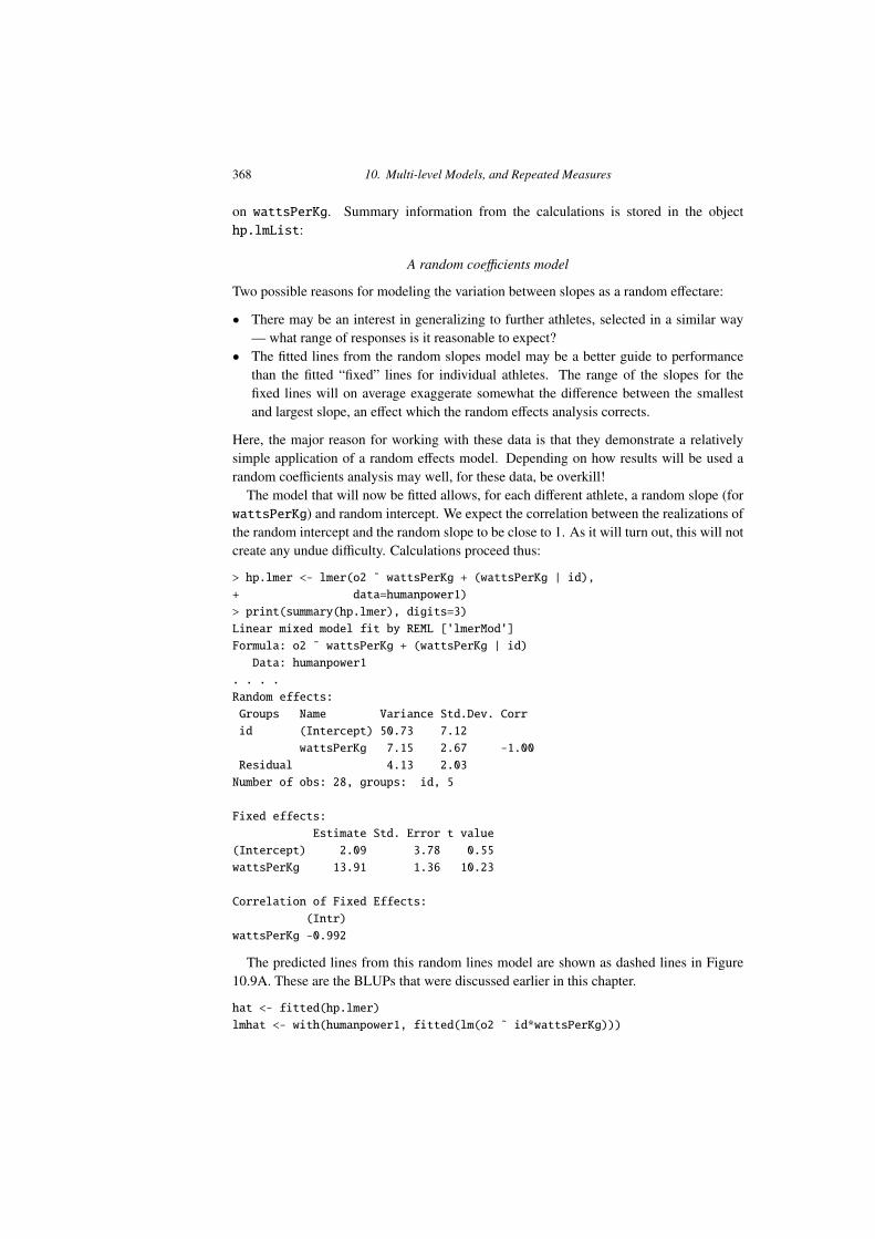
368 10. Multi-level Models, and Repeated Measures
on wattsPerKg. Summary information from the calculations is stored in the objecthp.lmList:
A random coe�cients model
Two possible reasons for modeling the variation between slopes as a random e↵ectare:
• There may be an interest in generalizing to further athletes, selected in a similar way— what range of responses is it reasonable to expect?
• The fitted lines from the random slopes model may be a better guide to performancethan the fitted “fixed” lines for individual athletes. The range of the slopes for thefixed lines will on average exaggerate somewhat the di↵erence between the smallestand largest slope, an e↵ect which the random e↵ects analysis corrects.
Here, the major reason for working with these data is that they demonstrate a relativelysimple application of a random e↵ects model. Depending on how results will be used arandom coe�cients analysis may well, for these data, be overkill!
The model that will now be fitted allows, for each di↵erent athlete, a random slope (forwattsPerKg) and random intercept. We expect the correlation between the realizations ofthe random intercept and the random slope to be close to 1. As it will turn out, this will notcreate any undue di�culty. Calculations proceed thus:
> hp.lmer <- lmer(o2 ˜ wattsPerKg + (wattsPerKg | id),
+ data=humanpower1)
> print(summary(hp.lmer), digits=3)
Linear mixed model fit by REML ['lmerMod']
Formula: o2 ˜ wattsPerKg + (wattsPerKg | id)
Data: humanpower1
. . . .
Random effects:
Groups Name Variance Std.Dev. Corr
id (Intercept) 50.73 7.12
wattsPerKg 7.15 2.67 -1.00
Residual 4.13 2.03
Number of obs: 28, groups: id, 5
Fixed effects:
Estimate Std. Error t value
(Intercept) 2.09 3.78 0.55
wattsPerKg 13.91 1.36 10.23
Correlation of Fixed Effects:
(Intr)
wattsPerKg -0.992
The predicted lines from this random lines model are shown as dashed lines in Figure10.9A. These are the BLUPs that were discussed earlier in this chapter.
hat <- fitted(hp.lmer)
lmhat <- with(humanpower1, fitted(lm(o2 ˜ id*wattsPerKg)))
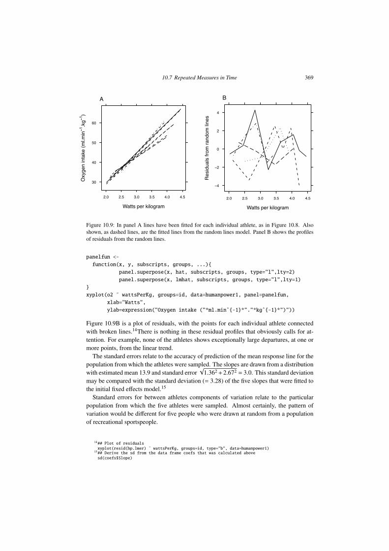
10.7 Repeated Measures in Time 369
Watts per kilogram
Oxy
gen
inta
ke (m
l.min−−1
.kg−−
1 )
30
40
50
60
2.0 2.5 3.0 3.5 4.0 4.5
A
Watts per kilogramRe
sidua
ls fro
m ra
ndom
lines
−4
−2
0
2
4
2.0 2.5 3.0 3.5 4.0 4.5
B
Figure 10.9: In panel A lines have been fitted for each individual athlete, as in Figure 10.8. Alsoshown, as dashed lines, are the fitted lines from the random lines model. Panel B shows the profilesof residuals from the random lines.
panelfun <-
function(x, y, subscripts, groups, ...){
panel.superpose(x, hat, subscripts, groups, type="l",lty=2)
panel.superpose(x, lmhat, subscripts, groups, type="l",lty=1)
}
xyplot(o2 ˜ wattsPerKg, groups=id, data=humanpower1, panel=panelfun,
xlab="Watts",
ylab=expression("Oxygen intake ("*ml.minˆ{-1}*"."*kgˆ{-1}*")"))
Figure 10.9B is a plot of residuals, with the points for each individual athlete connectedwith broken lines.14There is nothing in these residual profiles that obviously calls for at-tention. For example, none of the athletes shows exceptionally large departures, at one ormore points, from the linear trend.
The standard errors relate to the accuracy of prediction of the mean response line for thepopulation from which the athletes were sampled. The slopes are drawn from a distributionwith estimated mean 13.9 and standard error
p1.362+2.672 = 3.0. This standard deviation
may be compared with the standard deviation (= 3.28) of the five slopes that were fitted tothe initial fixed e↵ects model.15
Standard errors for between athletes components of variation relate to the particularpopulation from which the five athletes were sampled. Almost certainly, the pattern ofvariation would be di↵erent for five people who were drawn at random from a populationof recreational sportspeople.
14## Plot of residualsxyplot(resid(hp.lmer) ˜ wattsPerKg, groups=id, type="b", data=humanpower1)
15## Derive the sd from the data frame coefs that was calculated abovesd(coefs$Slope)
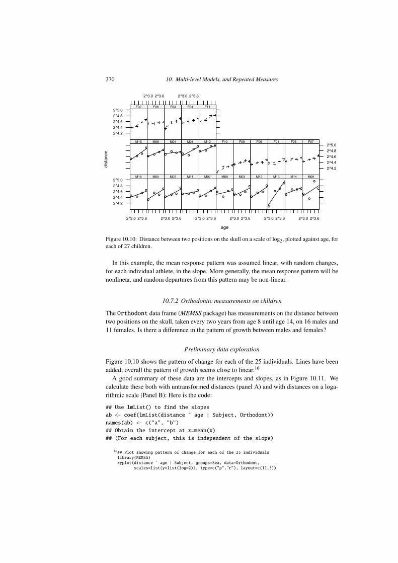
370 10. Multi-level Models, and Repeated Measures
age
distance
2^4.22^4.42^4.62^4.82^5.0
2^3.0 2^3.6
● ●
●●
M16
●
●●
●
M05
2^3.0 2^3.6
●● ●
●
M02
● ● ●●
M11
2^3.0 2^3.6
● ●
●
●
M07
●
●
●●
M08
2^3.0 2^3.6
● ●●
●
M03
●
● ●
●
M12
2^3.0 2^3.6
●
●●
●
M13
●
● ● ●
M14
2^3.0 2^3.6
●
●
●
●
M09
●●
●
●
M15
●●
●●
M06
●
●● ●
M04
●●
●●
M01
● ●
● ●
M10 F10 F09 F06 F01 F05
2^4.22^4.42^4.62^4.82^5.0
F07
2^4.22^4.42^4.62^4.82^5.0
F02
2^3.0 2^3.6
F08 F03
2^3.0 2^3.6
F04 F11
Figure 10.10: Distance between two positions on the skull on a scale of log2, plotted against age, foreach of 27 children.
In this example, the mean response pattern was assumed linear, with random changes,for each individual athlete, in the slope. More generally, the mean response pattern will benonlinear, and random departures from this pattern may be non-linear.
10.7.2 Orthodontic measurements on chlldren
The Orthodont data frame (MEMSS package) has measurements on the distance betweentwo positions on the skull, taken every two years from age 8 until age 14, on 16 males and11 females. Is there a di↵erence in the pattern of growth between males and females?
Preliminary data exploration
Figure 10.10 shows the pattern of change for each of the 25 individuals. Lines have beenadded; overall the pattern of growth seems close to linear.16
A good summary of these data are the intercepts and slopes, as in Figure 10.11. Wecalculate these both with untransformed distances (panel A) and with distances on a loga-rithmic scale (Panel B): Here is the code:
## Use lmList() to find the slopes
ab <- coef(lmList(distance ˜ age | Subject, Orthodont))
names(ab) <- c("a", "b")
## Obtain the intercept at x=mean(x)
## (For each subject, this is independent of the slope)
16## Plot showing pattern of change for each of the 25 individualslibrary(MEMSS)xyplot(distance ˜ age | Subject, groups=Sex, data=Orthodont,
scales=list(y=list(log=2)), type=c("p","r"), layout=c(11,3))
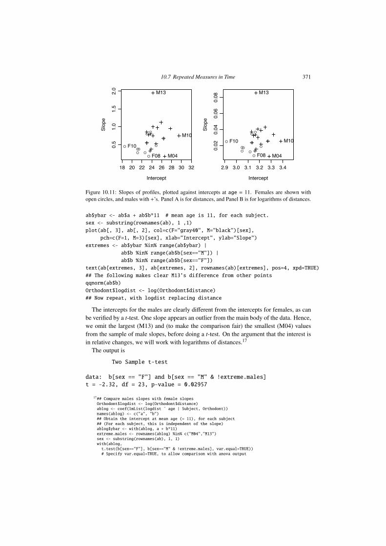
10.7 Repeated Measures in Time 371
●
●●●
●
●
●
●
●
●
●
18 20 22 24 26 28 30 32
0.5
1.0
1.5
2.0
Intercept
Slope
M13
M04
M10
F10
F08
●
●●●
●
●
●
●
●
●
●
2.9 3.0 3.1 3.2 3.3 3.4
0.02
0.04
0.06
0.08
Intercept
Slope
M13
M04
M10F10
F08
Figure 10.11: Slopes of profiles, plotted against intercepts at age = 11. Females are shown withopen circles, and males with +’s. Panel A is for distances, and Panel B is for logarithms of distances.
ab$ybar <- ab$a + ab$b*11 # mean age is 11, for each subject.
sex <- substring(rownames(ab), 1 ,1)
plot(ab[, 3], ab[, 2], col=c(F="gray40", M="black")[sex],
pch=c(F=1, M=3)[sex], xlab="Intercept", ylab="Slope")
extremes <- ab$ybar %in% range(ab$ybar) |
ab$b %in% range(ab$b[sex=="M"]) |
ab$b %in% range(ab$b[sex=="F"])
text(ab[extremes, 3], ab[extremes, 2], rownames(ab)[extremes], pos=4, xpd=TRUE)
## The following makes clear M13's difference from other points
qqnorm(ab$b)
Orthodont$logdist <- log(Orthodont$distance)
## Now repeat, with logdist replacing distance
The intercepts for the males are clearly di↵erent from the intercepts for females, as canbe verified by a t-test. One slope appears an outlier from the main body of the data. Hence,we omit the largest (M13) and (to make the comparison fair) the smallest (M04) valuesfrom the sample of male slopes, before doing a t-test. On the argument that the interest isin relative changes, we will work with logarithms of distances.17
The output is
Two Sample t-test
data: b[sex == "F"] and b[sex == "M" & !extreme.males]t = -2.32, df = 23, p-value = 0.02957
17## Compare males slopes with female slopesOrthodont$logdist <- log(Orthodont$distance)ablog <- coef(lmList(logdist ˜ age | Subject, Orthodont))names(ablog) <- c("a", "b")## Obtain the intercept at mean age (= 11), for each subject## (For each subject, this is independent of the slope)ablog$ybar <- with(ablog, a + b*11)extreme.males <- rownames(ablog) %in% c("M04","M13")sex <- substring(rownames(ab), 1, 1)with(ablog,t.test(b[sex=="F"], b[sex=="M" & !extreme.males], var.equal=TRUE))# Specify var.equal=TRUE, to allow comparison with anova output
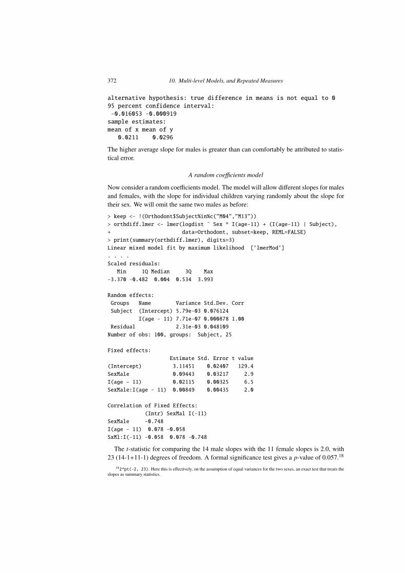
372 10. Multi-level Models, and Repeated Measures
alternative hypothesis: true difference in means is not equal to 095 percent confidence interval:-0.016053 -0.000919sample estimates:mean of x mean of y0.0211 0.0296
The higher average slope for males is greater than can comfortably be attributed to statis-tical error.
A random coe�cients model
Now consider a random coe�cients model. The model will allow di↵erent slopes for malesand females, with the slope for individual children varying randomly about the slope fortheir sex. We will omit the same two males as before:
> keep <- !(Orthodont$Subject%in%c("M04","M13"))
> orthdiff.lmer <- lmer(logdist ˜ Sex * I(age-11) + (I(age-11) | Subject),
+ data=Orthodont, subset=keep, REML=FALSE)
> print(summary(orthdiff.lmer), digits=3)
Linear mixed model fit by maximum likelihood ['lmerMod']
. . . .
Scaled residuals:
Min 1Q Median 3Q Max
-3.370 -0.482 0.004 0.534 3.993
Random effects:
Groups Name Variance Std.Dev. Corr
Subject (Intercept) 5.79e-03 0.076124
I(age - 11) 7.71e-07 0.000878 1.00
Residual 2.31e-03 0.048109
Number of obs: 100, groups: Subject, 25
Fixed effects:
Estimate Std. Error t value
(Intercept) 3.11451 0.02407 129.4
SexMale 0.09443 0.03217 2.9
I(age - 11) 0.02115 0.00325 6.5
SexMale:I(age - 11) 0.00849 0.00435 2.0
Correlation of Fixed Effects:
(Intr) SexMal I(-11)
SexMale -0.748
I(age - 11) 0.078 -0.058
SxMl:I(-11) -0.058 0.078 -0.748
The t-statistic for comparing the 14 male slopes with the 11 female slopes is 2.0, with23 (14-1+11-1) degrees of freedom. A formal significance test gives a p-value of 0.057.18
182*pt(-2, 23). Here this is e↵ectively, on the assumption of equal variances for the two sexes, an exact test that treats theslopes as summary statistics.
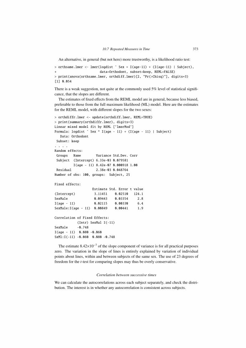
10.7 Repeated Measures in Time 373
An alternative, in general (but not here) more trustworthy, is a likelihood ratio test:
> orthsame.lmer <- lmer(logdist ˜ Sex + I(age-11) + (I(age-11) | Subject),
+ data=Orthodont, subset=keep, REML=FALSE)
> print(anova(orthsame.lmer, orthdiff.lmer)[2, "Pr(>Chisq)"], digits=3)
[1] 0.054
There is a weak suggestion, not quite at the commonly used 5% level of statistical signifi-cance, that the slopes are di↵erent.
The estimates of fixed e↵ects from the REML model are in general, because less biased,preferable to those from the full maximum likelihood (ML) model. Here are the estimatesfor the REML model, with di↵erent slopes for the two sexes:
> orthdiffr.lmer <- update(orthdiff.lmer, REML=TRUE)
> print(summary(orthdiffr.lmer), digits=3)
Linear mixed model fit by REML ['lmerMod']
Formula: logdist ˜ Sex * I(age - 11) + (I(age - 11) | Subject)
Data: Orthodont
Subset: keep
. . . .
Random effects:
Groups Name Variance Std.Dev. Corr
Subject (Intercept) 6.33e-03 0.079581
I(age - 11) 8.42e-07 0.000918 1.00
Residual 2.38e-03 0.048764
Number of obs: 100, groups: Subject, 25
Fixed effects:
Estimate Std. Error t value
(Intercept) 3.11451 0.02510 124.1
SexMale 0.09443 0.03354 2.8
I(age - 11) 0.02115 0.00330 6.4
SexMale:I(age - 11) 0.00849 0.00441 1.9
Correlation of Fixed Effects:
(Intr) SexMal I(-11)
SexMale -0.748
I(age - 11) 0.080 -0.060
SxMl:I(-11) -0.060 0.080 -0.748
The estimate 8.42⇥10�7 of the slope component of variance is for all practical purposeszero. The variation in the slope of lines is entirely explained by variation of individualpoints about lines, within and between subjects of the same sex. The use of 23 degrees offreedom for the t-test for comparing slopes may thus be overly conservative.
Correlation between successive times
We can calculate the autocorrelations across each subject separately, and check the distri-bution. The interest is in whether any autocorrelation is consistent across subjects.

374 10. Multi-level Models, and Repeated Measures
> res <- resid(orthdiffr.lmer)
> Subject <- factor(Orthodont$Subject[keep])
> orth.acf <- t(sapply(split(res, Subject),
+ function(x)acf(x, lag=4, plot=FALSE)$acf))
> ## Calculate respective proportions of Subjects for which
> ## autocorrelations at lags 1, 2 and 3 are greater than zero.
> apply(orth.acf[,-1], 2, function(x)sum(x>0)/length(x))
[1] 0.20 0.24 0.40
Thus a test for a zero lag 1 autocorrelation has p = 0.20. The suggestion of non-zeroautocorrelation is very weakly supported.
*The variance for the di↵erence in slopes
This can be calculated from the components of variance information. The sum of squaresabout the mean, for one line, is
P(x� x)2 = 20. The sum of the two components of variance
for an individual line is then: 1.19⇥10�12+0.002383/20= 0.00011915. The standard errorof the di↵erence in slopes is then:
p0.00011915(1/14+1/11) = 0.00440
Compare this with the value given against the fixed e↵ect SexMale:I(age - 11) in theoutput above. The numbers are, to within rounding error, the same. Degrees of freedomfor the comparison are 23 as for the t-test.
10.8 Further Notes on Multi-level and Other Models with Correlated Errors
10.8.1 Di↵erent sources of variance – complication or focus of interest?
In the discussion of multi-level models, the main interest was in the parameter estimates.The di↵erent sources of variance, were a complication. In other applications, the variancesmay be the focus of interest. Many animal and plant breeding trials are of this type. Theaim may be to design a breeding program that will lead to an improved variety or breed.Where there is substantial genetic variability, breeding experiments have a good chance ofcreating improved varieties.
Investigations into the genetic component of human intelligence have generated fiercedebate. Most such studies have used data from identical twins who have been adopted outto di↵erent homes, comparing them with non-identical twins and with sibs who have beensimilarly adopted out. The adopting homes rarely span a large part of a range from extremesocial deprivation to social privilege, so that results from such studies may have little or norelevance to investigation of the e↵ects of extreme social deprivation. The discussion inLeavitt and Dubner (2005, chapter 5) sheds interesting light on these these e↵ects.
There has not been, until recently, proper allowance for the substantial e↵ects that arisefrom simultaneous or sequential occupancy of the maternal womb (Bartholemew, 2004;Daniels et al., 1997). Simple forms of components of variance model are unable to accountfor the Flynn e↵ect (Bartholemew, 2004, pp. 138-140), by which measured IQs in manyparts of the world have in recent times increased by about 15 IQ points per generation. The

10.8 Further Notes on Multi-level and Other Models with Correlated Errors 375
simple model, on which assessments of proportion of variance that is genetic have beenbased, seems too simplistic to give useful insight.
We have used an analysis of data from a field experimental design to demonstrate thecalculation and use of components of variance. Other contexts for multi-level models arethe analysis of data from designed surveys, and general regression models in which the“error” term is made up of several components. In all these cases, errors are no longerindependently and identically distributed.
10.8.2 Predictions from models with a complex error structure
Here, “complex” refers to models that assume something other than an i.i.d. error structure.Most of the models considered in this chapter can be used for di↵erent predictive purposes,and give standard errors for predicted values that di↵er according to the intended purpose.Accurate modeling of the structure of variation allows, as for the Antiguan corn yield datain Section 10.1), these di↵erent inferential uses.
As has been noted, shortcuts are sometimes possible. Thus for using the kiwifruit shad-ing data to predict yields at any level other than the individual vine, there is no loss ofinformation from basing the analysis on plot means.
Consequences from assuming an overly simplistic error structure
In at least some statistical application areas, analyses that assume an overly simplisticerror structure (usually, an i.i.d. model) are relatively common in the literature. Inferencesmay be misleading, or not, depending on how results are used. Where there are multiplelevels of variation, all variation that contributes to the sampling error of fixed e↵ects mustbe modeled correctly. Otherwise, the standard errors of model parameters that appear incomputer output will almost inevitably be wrong, and should be ignored.
In data that have appropriate balance, predicted values will ordinarily be unbiased, evenif the error structure is not modeled appropriately. The standard errors will almost certainlybe wrong, usually optimistic. A good understanding of the structure of variation is typicallyrequired in order to make such limited inferences as are available when an overly simplisticerror structure is assumed!
10.8.3 An historical perspective on multi-level models
Multi-level models are not new. The inventor of the analysis of variance was R.A. Fisher.Although he would not have described it that way, many of the analysis of variance cal-culations that he demonstrated were analyses of specific forms of multi-level model. Datahave a structure that is imposed by the experimental design. The particular characteristicof the experimental design models that Fisher used was that the analysis could be handledusing analysis of variance methods. The variance estimates that are needed for di↵erentcomparisons may be taken from di↵erent lines of the analysis of variance table. This cir-cumvents the need to estimate the variances of the random e↵ects that appear in a fullygeneral analysis.
Until the modern computing era, multi-level data whose structure did not follow one of
376 10. Multi-level Models, and Repeated Measures
the standard designs and thus did not fit the analysis of variance framework required someform of approximate analysis. Such approximate analyses, if they were possible at all,often demanded a high level of skill.
Statistical analysts who used Fisher’s experimental designs and methods of analysis fol-lowed Fisher’s rules, and those of his successors, for the calculations. Each di↵erent designhad its own recipe. After working through a few such analyses, some of those who fol-lowed Fisher’s methods began to feel that they understood the rationale fairly well at anintuitive level. Books appeared that gave instructions on how to do the analyses. The mostcomprehensive of these is Cochran and Cox (1957).
The Genstat system (Payne et al., 1997) was the first of the major systems to implementgeneral methods for the analysis of multi-level models that had a suitable “balance”. Itscoherent and highly structured approach to the analysis of data from suitably balanceddesigns takes advantage of the balance to simplify and structure the output.
General purpose software for use with unbalanced data, in the style of the lme4 package,made its appearance relatively recently. The analyses that resulted from earlier ad hocapproaches were in general less insightful and informative than the more adequate analysesthat are available within a multi-level modeling framework.
Regression models are another starting point for consideration of multi-level models.Both the fixed e↵ects parts of the model have a structure, thus moving beyond the mod-els with a single random (or “error”) term that have been the stock in trade of courses onregression modeling. Even now, most regression texts give scant recognition of the impli-cations of structure in the random part of the model. Yet data commonly do have structure– students within classes within institutions, nursing sta↵ within hospitals within regions,managers within local organizations within regional groupings, and so on.
As has been noted, models have not always been written down. Once theoretical statis-ticians did start to write down models, there was a preoccupation with models that had asingle error term. Theoretical development, where the discussion centered around models,was disconnected from the practical analysis of experimental designs, where most analystswere content to follow Cochran and Cox and avoid formal mathematical description of themodels that underpinned their analyses.
Observational data that have a multilevel structure, which is typically unbalanced, cannowadays be analyzed just as easily as experimental data. It is no longer necessary to lookup Cochran and Cox to find how to do an analysis. There are often acceptable alternativesto Cochran and Cox style experimental designs.
Problems of interpretation and meaningfulness remain, for observational data, as di�-cult as ever. The power of modern software can become a trap. There may be inadequatecare in the design of data collection, in the expectation that computer software will takecare of any problems. The result may be data whose results are hard to interpret or cannotbe interpreted at all, or that make poor use of resources.
10.8.4 Meta-analysis
Meta-analysis is a name for analyses that bring together into a single analysis frameworkdata from, for example, multiple agricultural trials, or from multiple clinical trials, or frommultiple psychological laboratories. Multi-level modeling, and extensions of multi-levelmodeling such as repeated measures analysis, make it possible to do analyses that take
10.9 Recap 377
proper account of site to site or center to center or study to study variation. If treatment orother e↵ects are consistent relative to all identifiable major sources of variation, the resultcan be compelling for practical application.
Meta-analysis is uncontroversial when data are from a carefully planned multi-locationtrial. More controversial is the bringing together into one analysis of data from quite sepa-rate investigations. There may however be little choice; the alternative may be an informaland perhaps unconvincing qualitative evaluation of the total body of evidence. Clearlysuch analyses challenge the critical acumen of the analyst. A wide range of methodologieshave been developed to handle the problems that may arise. Gaver et al. (1992) is a usefulsummary. Turner et al. (2009) is an interesting and comprehensive state-of-the-art account.
10.8.5 Functional data analysis
Much of the art of repeated measures modeling lies in finding suitable representations,requiring a small number of parameters, both of the individual profiles and of variation be-tween those profiles. Spline curves are widely used in this context. Chapter 12 will discussthe use of principal components to give a low-dimensional representation of multivariatedata. A similar methodology can be used to find representations of curves in terms of asmall number of basis functions. Further details are in Ramsay and Silverman (2002).
10.8.6 Error structure in explanatory variables
This chapter has discussed error structure in response variables. There may also be a struc-ture to error in explanatory variables. Studies of the health e↵ects of dietary components,such as were described in Subsection 6.8, provide an interesting and important example,with major implications for the design of such studies.
10.9 Recap
Multi-level models account for multiple levels of random variation. The random part ofthe model possesses structure; it is a sum of distinct random components.
In making predictions based on multi-level models, it is necessary to identify preciselythe population to which the predictions will apply.
The art in setting up an analysis for these models is in getting the description of themodel correct. Specifically it is necessary to
• identify which are fixed and which random e↵ects,• correctly specify the nesting of the random e↵ects.
In repeated measures designs, it is necessary to specify or otherwise model the patternof correlation within profiles.
A further generalization is to the modeling of random coe�cients, for example, regres-sion lines that vary between di↵erent subsets of the data.
Skill and care may be needed to get output into a form that directly addresses the ques-tions that are of interest. Finally, output must be interpreted. Multi-level analyses oftenrequire high levels of professional skill.
378 10. Multi-level Models, and Repeated Measures
10.10 Further Reading
Fisher (1935) is a non-mathematical account that takes the reader step by step through theanalysis of important types of experimental design. It is useful background for readingmore modern accounts. Williams et al. (2002) is similarly example-based, with an em-phasis on tree breeding. See also Cox (1958); Cox and Reid (2000). Cox and Reid is anauthoritative up to date account of the area, with a more practical focus than its title mightseem to imply. On multi-level and repeated measures models see Gelman and Hill (2007);Snijders and Bosker (1999); Diggle et al. (2002); Goldstein (1995); Pinheiro and Bates(2000); Venables and Ripley (2002).
Talbot (1984) is an interesting example of the use of multi-level modeling, with impor-tant agricultural and economic implications. It summarizes a large amount of informationthat is of importance to farmers, on yields for many di↵erent crops in the UK, includingassessments both of center to center and of year to year variation.
The relevant chapters in Payne et al. (1997), while directed to users of the Genstat sys-tem, have helpful commentary on the use of the methodology and on the interpretationof results. Pinheiro and Bates (2000) describes the use of the nlme package for handlingmulti-level analyses.
On meta-analysis see Chalmers and Altman (1995); Gaver et al. (1992); Turner et al.(2009).
References for further reading
Analysis of variance with multiple error terms
Cochran, W.G. and Cox, G.M. 1957. Experimental Designs, 2nd edn.Cox, D.R. 1958. Planning of Experiments.Cox, D.R. and Reid, N. 2000. Theory of the Design of Experiments.Fisher, R.A. 1935 (7th edn. 1960). The Design of Experiments.Payne, R.W., Lane, P.W., Digby, P.G.N., Harding, S.A., Leech, P.K., Morgan, G.W.,
Todd, A.D., Thompson, R., Tunnicli↵e Wilson, G., Welham, S.J. and White, R.P. 1997.Genstat 5 Release 3 Reference Manual.
Williams, E.R., Matheson, A.C. and Harwood, C.E. 2002. Experimental Design and Anal-ysis for Use in Tree Improvement, revised edn.
Multi-level models and repeated measures
Diggle, P.J., Heagerty, P.J., Liang, K.-Y. and Zeger, S.L. 2002. Analysis of LongitudinalData, 2nd edn.
Gelman, A. and Hill, J., 2007. Data analysis using regression and multilevel/hierarchicalmodels.
Goldstein, H. 1995. Multi-level Statistical Models.Payne, R.W., Lane, P.W., Digby, P.G.N., Harding, S.A., Leech, P.K., Morgan, G.W.,
Todd, A.D., Thompson, R., Tunnicli↵e Wilson, G., Welham, S.J. and White, R.P. 1993.Genstat 5 Release 3 Reference Manual.
Pinheiro, J.C. and Bates, D.M. 2000. Mixed E↵ects Models in S and S-PLUS.
10.11 Exercises 379
Snijders, T.A.B. and Bosker, R.J. 1999. Multilevel Analysis. An Introduction to Basic andAdvanced Multilevel Modelling.
Talbot, M. 1984. Yield variability of crop varieties in the UK. Journal of the AgriculturalSociety of Cambridge 102: 315–321. JRSS A 172: 21-47.
Venables, W.N. and Ripley, B.D. 2002. Modern Applied Statistics with S, 4th edn.
Meta-analysis
Chalmers, I. and Altman, D.G. 1995. Systematic Reviews.Gaver, D.P., Draper, D.P., Goel, K.P., Greenhouse, J.B., Hedges, L.V., Morris, C.N. and
Waternaux, C. 1992. Combining Information: Statistical Issues and Opportunities forResearch.
Turner et al. 2009. Bias modelling in evidence synthesis.
10.11 Exercises
1. Repeat the calculations of Subsection 10.4.5, but omitting results from two vines at random.Here is code that will handle the calculation:n.omit <- 2
take <- rep(TRUE, 48)
take[sample(1:48,2)] <- FALSE
kiwishade.lmer <- lmer(yield ˜ shade + (1|block) + (1|block:plot),
data = kiwishade,subset=take)
vcov <- VarCorr(kiwishade.lmer)
print(vcov, comp="Variance")Repeat this calculation five times, for each of n.omit = 2, 4, 6, 8, 10, 12 and 14. Plot (i) the plotcomponent of variance and (ii) the vine component of variance, against number of points omitted.Based on these results, for what value of n.omit does the loss of vines begin to compromiseresults? Which of the two components of variance estimates is more damaged by the loss ofobservations? Comment on why this is to be expected.
2. Repeat the previous exercise, but now omitting 1, 2, 3, 4 complete plots at random.
3. The data set Gun (MEMSS package) reports on the numbers of rounds fired per minute, by eachof nine teams of gunners, each tested twice using each of two methods. In the nine teams, threewere made of men with slight build, three with average, and three with heavy build. Is there adetectable di↵erence, in number of rounds fired, between build type or between firing methods?For improving the precision of results, which would be better – to double the number of teams,or to double the number of occasions (from 2 to 4) on which each team tests each method?
4. *The data set ergoStool (MEMSS package) has data on the amount of e↵ort needed to get upfrom a stool, for each of nine individuals who each tried four di↵erent types of stool. Analyzethe data both using aov() and using lme(), and reconcile the two sets of output. Was there anyclear winner among the types of stool, if the aim is to keep e↵ort to a minimum?
5. *In the data set MathAchieve (MEMSS package), the factors Minority (levels yes and no)and sex, and the variable SES (socio-economic status) are clearly fixed e↵ects. Discuss how thedecision whether to treat School as a fixed or as a random e↵ect might depend on the purpose ofthe study? Carry out an analysis that treats School as a random e↵ect. Are di↵erences between
380 10. Multi-level Models, and Repeated Measures
schools greater than can be explained by within school variation?
6. *The data frame sorption (DAAG) includes columns ct (concentration-time sum), Cultivar(apple cultivar), Dose (injected dose of methyl bromide), and rep (replicate number, withinCultivar and year). Fit a model that allows the slope of the regression of ct on Dose to bedi↵erent for di↵erent cultivars and years. and to vary randomly with replicate. Consider the twomodels:cult.lmer <- lmer(ct ˜ Cultivar + Dose + factor(year) +
(-1 + Dose | gp), data = sorption,
REML=TRUE)
cultdose.lmer <- lmer(ct ˜ Cultivar/Dose + factor(year) +
(-1 + Dose | gp), data = sorption,
REML=TRUE)
Explain (i) the role of the each of the terms in these models, and (ii) how the two models di↵er.Which model seems preferable? Write a brief commentary on the output from the preferredmodel.[NB: The factor gp, which has a di↵erent level for each di↵erent combination of Cultivar,year and replicate, associates a di↵erent random e↵ect with each such combination.]