Multi-Manifold Semi-Supervised Learning

Multi-Manifold Semi-Supervised Learning

†Computer Sciences Dept.University of Wisconsin-Madison

Madison, WI 53706, USAgoldberg,jerryzhu,zhiting

@cs.wisc.edu

Andrew B. Goldberg† Xiaojin Zhu† Aarti Singh‡ Zhiting Xu† Robert Nowak∗‡Applied and Computational Math

Princeton UniversityPrinceton, NJ 08544, [email protected]

∗Elec. and Computer EngineeringUniversity of Wisconsin-Madison

Madison, WI 53706, [email protected]

Abstract

We study semi-supervised learning when thedata consists of multiple intersecting mani-folds. We give a finite sample analysis toquantify the potential gain of using unlabeleddata in this multi-manifold setting. We thenpropose a semi-supervised learning algorithmthat separates different manifolds into deci-sion sets, and performs supervised learningwithin each set. Our algorithm involves anovel application of Hellinger distance andsize-constrained spectral clustering. Exper-iments demonstrate the benefit of our multi-manifold semi-supervised learning approach.

1 INTRODUCTION

The promising empirical success of semi-supervisedlearning algorithms in favorable situations has trig-gered several recent attempts (Balcan & Blum 2005,Ben-David, Lu & Pal 2008, Kaariainen 2005, Laf-ferty & Wasserman 2007, Niyogi 2008, Rigollet 2007)at developing a theoretical understanding of semi-supervised learning. In a recent paper (Singh, Nowak& Zhu 2008), it was established using a finite sam-ple analysis that if the complexity of the distribu-tions under consideration is too high to be learnt us-ing n labeled data points, but is small enough tobe learnt using m n unlabeled data points, thensemi-supervised learning (SSL) can improve the per-formance of a supervised learning (SL) task. Therehave also been many successful practical SSL algo-rithms as summarized in (Chapelle, Zien & Scholkopf2006, Zhu 2005). These theoretical analyses and prac-

Appearing in Proceedings of the 12th International Confe-rence on Artificial Intelligence and Statistics (AISTATS)2009, Clearwater Beach, Florida, USA. Volume 5 of JMLR:W&CP 5. Copyright 2009 by the authors.

tical algorithms often assume that the data forms clus-ters or resides on a single manifold.

However, both a theory and an algorithm are lackingwhen the data is supported on a mixture of manifolds.Such data occurs naturally in practice. For instance,in handwritten digit recognition each digit forms itsown manifold in the feature space; in computer visionmotion segmentation, moving objects trace differenttrajectories which are low dimensional manifolds (Tron& Vidal 2007). These manifolds may intersect or par-tially overlap, while having different dimensionality,orientation, and density. Existing SSL approaches can-not be directly applied to multi-manifold data. Forinstance, traditional graph-based SSL algorithms maycreate a graph that connects points on different mani-folds near a manifold intersection, thus diffusing infor-mation across the wrong manifolds.

In this paper, we generalize the theoretical analysisof (Singh et al. 2008) to the case where the data is sup-ported on a mixture of manifolds. Guided by the the-ory, we propose an SSL algorithm that handles multi-ple manifolds as well as clusters. The algorithm buildsupon novel Hellinger-distance-based graphs and size-constrained manifold clustering. Experiments showthat our algorithm can perform SSL on multiple in-tersecting, overlapping, and noisy manifolds.

2 THEORETIC PERSPECTIVES

In this section, we first review the conclusions of (Singhet al. 2008), which are based on the cluster assump-tion, and then give conjectured bounds in the singlemanifold and multi-manifold case.

The cluster assumption, as formulated in (Singh et al.2008), states that the target regression function orclass label is locally smooth over certain subsets ofthe D-dimensional feature space that are delineated bychanges in the marginal density—throughout this pa-per, we assume the marginal density is bounded above


and below (away from zero). We refer to these delin-eated subsets as decision sets; i.e., all non-empty setsformed by intersections between the cluster supportsets and their complements. If these decision sets, de-noted by C, can be learnt using unlabeled data, thelearning task on each decision set is simplified. Theresults of (Singh et al. 2008) suggest that if the de-cision sets can be resolved using unlabeled data, butnot using labeled data, then semi-supervised learningcan help. However, this simple argument, and hencethe distinctions between SSL and SL, are not alwayscaptured by standard asymptotic arguments based onrates of convergence. (Singh et al. 2008) used finitesample bounds to characterize both the SSL gains andthe relative value of unlabeled data.

To derive the finite sample bounds, the first step isto understand when the decision sets are resolvableusing data. This depends on the interplay betweenthe complexity of the class of distributions under con-sideration and the number of unlabeled points m andlabeled points n. For the cluster case, the complex-ity of the distributions is determined by the marginγ, defined as the minimum separation between clus-ters or the minimum width of a decision set (Singhet al. 2008). If the margin γ is larger than the typi-cal distance between the data points (m−1/D if usingunlabeled data, or n−1/D if using only labeled data),then with high probability the decision sets can belearnt up to a high accuracy (which depends on m orn, respectively) (Singh et al. 2008). This implies thatif γ > m−1/D (margin exists with respect to densityof unlabeled data), then the finite sample performance(the expected excess error Err) of a semi-supervisedlearner fm,n relative to the performance of a clairvoy-ant supervised learner fC,n, which has perfect knowl-edge of the decision sets C, can be characterized asfollows:

supPXY (γ)

Err(fm,n) ≤ supPXY (γ)

Err(fC,n) + δ(m,n). (1)

Here PXY (γ) denotes the cluster-based class of distri-butions with complexity γ, and δ(m,n) is the error in-curred due to inaccuracies in learning the decision setsusing unlabeled data. Comparing this upper boundon the semi-supervised learning performance to a fi-nite sample minimax lower bound on the performanceof any supervised learner provides a sense of the rel-ative performance of SL vs. SSL. Thus, SSL helps ifcomplexity of the class of distributions γ > m−1/D

and both of the following conditions hold: (i) knowl-edge of decision sets simplifies the supervised learn-ing task, that is, the error of the clairvoyant learnersupPXY (γ) Err(fC,n) < inffn supPXY (γ) Err(fn), thesmallest error that can be achieved by any supervisedlearner based on n labeled data. The difference quan-

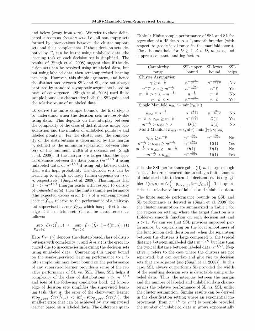
Table 1: Finite sample performance of SSL and SL forregression of a Holder-α, α > 1, smooth function (withrespect to geodesic distance in the manifold cases).These bounds hold for D ≥ 2, d < D, m n, andsuppress constants and log factors.

Complexity SSL upper SL lower SSLrange bound bound helps

Cluster Assumptionγ ≥ n−

1D n−

2α2α+D n−

2α2α+D No

n−1D > γ ≥ m− 1

D n−2α

2α+D n−1D Yes

m− 1D > γ ≥ −m− 1

D n−1D n−

1D No

−m− 1D > γ n−

2α2α+D n−

1D Yes

Single Manifold κSM := min(r0, s0)

κSM ≥ n−1D n−

2α2α+d n−

2α2α+d No

n−1D > κSM ≥ m− 1

D n−2α

2α+d Ω(1) Yesm− 1

D > κSM ≥ 0 O(1) Ω(1) NoMulti-Manifold κMM := sgn(γ) ·min(|γ|, r0, s0)

κMM ≥ n−1D n−

2α2α+d n−

2α2α+d No

n−1D > κMM ≥ m− 1

D n−2α

2α+d Ω(1) Yesm− 1

D > κMM ≥ −m− 1D O(1) Ω(1) No

−m− 1D > κMM n−

2α2α+d Ω(1) Yes

tifies the SSL performance gain. (ii) m is large enoughso that the error incurred due to using a finite amountof unlabeled data to learn the decision sets is negligi-ble: δ(m,n) = O

(supPXY (γ) Err(fC,n)

). This quan-

tifies the relative value of labeled and unlabeled data.

The finite sample performance bounds on SSL andSL performance as derived in (Singh et al. 2008) forthe cluster assumption are summarized in Table 1 forthe regression setting, where the target function is aHolder-α smooth function on each decision set andα > 1. We can see that SSL provides improved per-formance, by capitalizing on the local smoothness ofthe function on each decision set, when the separationbetween the clusters is large compared to the typicaldistance between unlabeled data m−1/D but less thanthe typical distance between labeled data n−1/D. Neg-ative γ refers to the case where the clusters are notseparated, but can overlap and give rise to decisionsets that are adjacent (see (Singh et al. 2008)). In thiscase, SSL always outperforms SL provided the widthof the resulting decision sets is detectable using unla-beled data. Thus, the interplay between the marginand the number of labeled and unlabeled data charac-terizes the relative performance of SL vs. SSL underthe cluster assumption. Similar results can be derivedin the classification setting where an exponential im-provement (from n−1/D to e−n) is possible providedthe number of unlabeled data m grows exponentially

Goldberg, Zhu, Singh, Xu, Nowak

with n (Singh et al. 2008).

2.1 SINGLE MANIFOLD CASE

In the single manifold case, the assumption is thatthe target function lies on a lower d-dimensional man-ifold, where d < D, and is Holder-α smooth (α > 1)with respect to the geodesic distance on the manifold.Hence knowledge of the manifold, or equivalently thegeodesic distances between all pairs of data points, canbe gleaned using unlabeled data and reduces the di-mensionality of the learning task.

In the case of distributions supported on a single man-ifold, the ability to learn the geodesic distances well,and hence the complexity κSM of the distributions, de-pends on two geometric properties of the manifold—its minimum radius of curvature r0 and proximity toself-intersection s0 (also known as branch separation)(Bernstein, de Silva, Langford & Tenenbaum 2000).If κSM := min(r0, s0) is larger than the typical dis-tance between the data points (m−1/D with unlabeleddata, or n−1/D with only labeled data), then with highprobability the manifold structure is resolvable andgeodesic distances can be learnt up to a high accuracy(which depends on m or n, respectively). This can beachieved by using shortest distance paths on an ε- ork-nearest neighbor graph to approximate the geodesicdistances (Bernstein et al. 2000). The use of approx-imate geodesic distances to learn the target functiongives rise to an error-in-variable problem. Though theoverall learning problem is now reduced to a lower-dimensional problem, we are now faced with two typesof errors—the label noise and the error in the esti-mated distances. However, the error incurred in thefinal estimation due to errors in geodesic distances de-pends on m which is assumed to be much greater thann. Thus, the effect of the geodesic distance errors isnegligible, compared to the error due to label noise,for m sufficiently large. This suggests that for themanifold case, if κSM > m−1/D, then finite sampleperformance of semi-supervised learning can again berelated to the performance of a clairvoyant supervisedlearner fC,n as in (1) above, since δ(m,n) is negligiblefor m sufficiently large.

Comparing this SSL performance bound to a finitesample minimax lower bound on the performance ofany supervised learner indicates SSL’s gain in the sin-gle manifold case and is summarized in Table 1. Theseare conjectured bounds based on the arguments aboveand similar arguments in (Niyogi 2008). The SSL up-per bound can be achieved using a learning procedureadaptive to both α and d, such as the method proposedin (Bickel & Li 2007)1. The SL lower bounds follow

1Note, however, that the analysis in (Bickel & Li 2007)

from the results in (Tsybakov 2004) and (Niyogi 2008).SSL provides improved performance by capitalizing onthe lower-dimensional structure of the manifold whenthe minimum radius of curvature and branch separa-tion are large compared to the typical distance be-tween unlabeled data m−1/D, but small compared tothe typical distance between labeled data n−1/D.

2.2 MULTI-MANIFOLD CASE

The multi-manifold case addresses the generic settingwhere the clusters are low-dimensional manifolds thatpossibly intersect or overlap. In this case, the targetfunction is supported on multiple manifolds and can bepiecewise smooth on each manifold. Thus, it is of in-terest to resolve the manifolds, as well as the subsets ofeach manifold where the decision label varies smoothly(that are characterized by changes in the marginal den-sity). The analysis for this case is a combination of thecluster and single manifold case. The complexity of themulti-manifold class of distributions, denoted κMM, isgoverned by the minimum of the manifold curvatures,branch separations, and the separations and overlapsbetween distinct manifolds. For the regression setting,the conjectured finite sample minimax analysis is pre-sented in Table 1.

These results indicate that when there is enough unla-beled data, but not enough labeled data, to handle thecomplexity of the class, then semi-supervised learningcan help by adapting to both the intrinsic dimensional-ity and smoothness of the target function. Extensionsof these results to the classification setting are straight-forward, as discussed under the cluster assumption.

3 AN ALGORITHM

Guided by the theoretical analysis in the previous sec-tion, we propose a “cluster-then-label” type of SSL al-gorithm, see Figure 1. It consists of three main steps:(1) It uses the unlabeled data to form a small num-ber of decision sets, on which the target function isassumed to be smooth. The decision sets are definedin the ambient space, not just on the labeled and unla-beled points. (2) The target function within a partic-ular decision set is estimated using only labeled datathat fall in that decision set, and using a supervisedlearner specified by the user. (3) a new test point ispredicted by the target function in the decision set itfalls into.

There have been several cluster-then-label approachesin the SSL literature. For example, the early workof Demiriz et al. modifies the objective of standard

considers the asymptotic performance of SL, whereas herewe are studying the finite-sample performance of SSL.


k-means clustering algorithms to include a class impu-rity term (Demiriz, Bennett & Embrechts 1999). El-Yaniv and Gerzon enumerate all spectral clusteringsof the unlabeled data with varying number of clusters,which together with labeled data induce a hypothesisspace. They then select the best hypothesis based onan Occam’s razor-type transductive bound (El-Yaniv& Gerzon 2005). Some work in “constrained cluster-ing” is also closely related to cluster-then-label froman SSL perspective (Basu, Davidson & Wagstaff 2008).Compared to these approaches, our algorithm has twoadvantages: i) it is supported by our SSL minimaxtheory; ii) it handles both overlapping clusters and in-tersecting manifolds by detecting changes in support,density, dimensionality or orientation.

Our algorithm is also different from the family ofgraph-regularized SSL approaches, such as manifoldregularization (Belkin, Sindhwani & Niyogi 2006)and earlier variants (Joachims 2003, Zhou, Bousquet,Lal, Weston & Scholkopf 2004, Zhu, Ghahramani &Lafferty 2003). Those approaches essentially add agraph-regularization term in the objective. They alsodepend on the “manifold assumption” that the targetfunction indeed varies smoothly on the manifold. Incontrast, i) our algorithm is a wrapper method, whichuses any user-specified supervised learner SL as a sub-routine. This allows us to directly take advantage ofadvances in supervised learning without the need toderive new algorithms. ii) Our theory ensures that,even when the manifold assumption is wrong, our SSLperformance bound is the same as that of the super-vised learner (up to a log factor).

Finally, step 1 of our algorithm is an instance of man-ifold clustering. Recent advances on this topic includeGeneralized Principal Component Analysis (Vidal, Ma& Sastry 2008) and lossy coding (Ma, Derksen, Hong& Wright 2007) for mixtures of linear subspaces, mul-tiscale manifold identification with algebraic multi-grid (Kushnir, Galun & Brandt 2006), tensor vot-ing (Mordohai & Medioni 2005), spectral curvatureclustering (Chen & Lerman 2008), and translated Pois-son mixture model (Haro, Randall & Sapiro 2008) formixtures of nonlinear manifolds. Our algorithm isunique in two ways: i) its use of Hellinger distanceoffers a new approach to detecting overlapping clus-ters and intersecting manifolds; ii) our decision setshave minimum size constraints, which we enforce byconstrained k-means.

3.1 HELLINGER DISTANCE GRAPH

Let the labeled data be (xi, yi)ni=1, and the unla-

beled data be xjMj=1, where M n. The build-

ing block of our algorithm is a local sample covari-ance matrix. For a point x, define N(x) to be

a small neighborhood around x in Euclidean space.Let Σx be the local sample covariance matrix at x:Σx =

∑x′∈N(x)(x

′−µx)(x′−µx)>/(|N(x)|−1), whereµx =

∑x′∈N(x) x′/|N(x)| is the neighborhood mean.

In our experiments, we let |N(x)| ∼ O(log(M)) so thatthe neighborhood size grows with unlabeled data sizeM . The covariance Σx captures the local geometryaround x.

Our intuition is that points xi, xj on different man-ifolds or in regions with different density should beconsidered dissimilar. This intuition is captured bythe Hellinger distance between their local sample co-variance matrices Σi,Σj . The squared Hellinger dis-tance is defined between two pdf’s p, q: H2(p, q) =12

∫ (√p(x)−

√q(x)

)2

dx. By setting p(x) =N (x; 0,Σi), i.e., a Gaussian with zero mean and co-variance Σi, and similarly q(x) = N (x; 0,Σj), we ex-tend the definition of Hellinger distance to covariancematrices: H(Σi,Σj) ≡ H (N (x; 0,Σi),N (x; 0,Σi)) =√

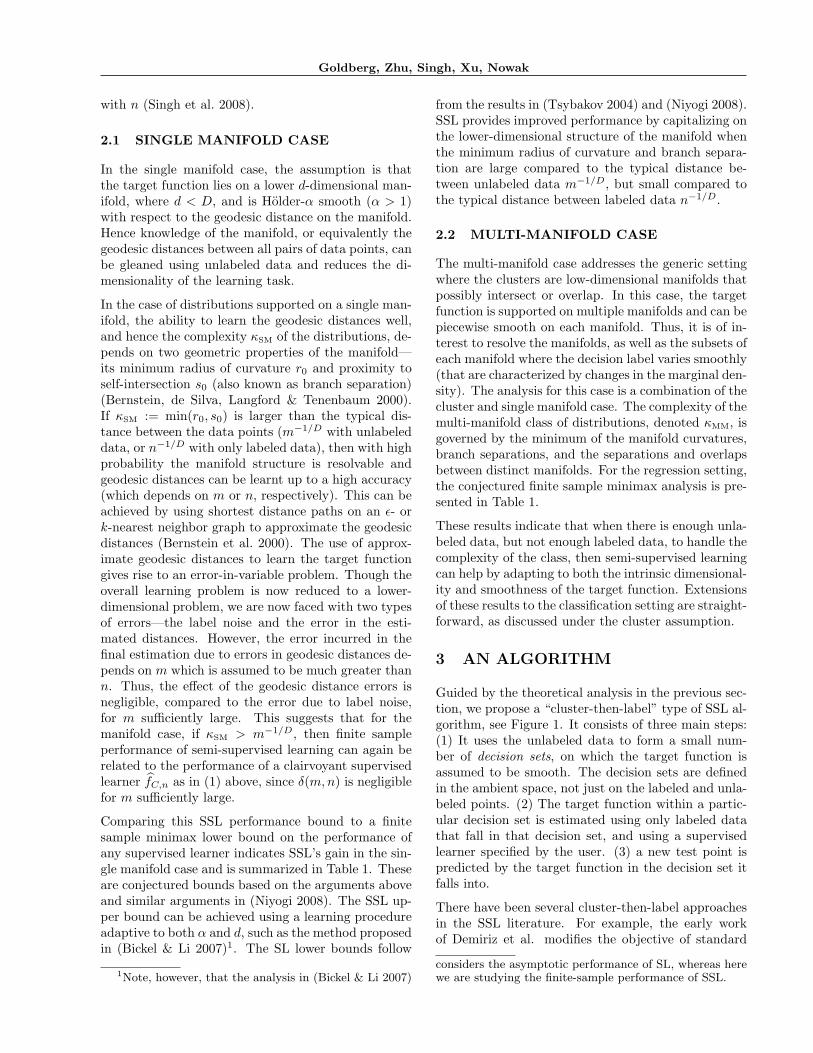
1− 2D/2|Σi|1/4|Σj |1/4/|Σi + Σj |1/2, where D is thedimensionality of the ambient feature space. We willalso call H(Σi,Σj) the Hellinger distance between thetwo points xi, xj . When Σi +Σj is rank deficient, H iscomputed in the subspace occupied by Σi + Σj . TheHellinger distance H is symmetric and in [0, 1]. His small when the local geometry is similar, and largewhen there is significant difference in density, manifolddimensionality or orientation. Example 3D covariancematrices and their H values are shown in Figure 2.

Cov. matrices Comment H(Σ1,Σ2)

similar 0.02

density 0.28

dimension 1

orientation 1

Figure 2: Hellinger distance

It would seem natural to compute all pairwiseHellinger distances between our dataset of n + Mpoints to form a graph, and apply a graph-cut algo-rithm to separate multiple manifolds or clusters. How-ever, if xi and xj are very close to each other, their lo-cal neighborhoods N(xi), N(xj) will strongly overlap.Then, even if the two points are on different manifoldsthe Hellinger distance will be small, because their co-variance matrices Σi,Σj will be similar. Therefore, weselect a subset of m ∼ O (M/ log(M)) unlabeled pointsso that they are farther apart while still covering thewhole dataset. This is done using a greedy procedure,


Given n labeled examples and M unlabeled examples, and a supervised learner SL,

1. Use the unlabeled data to infer k ∼ O(log(n)) decision sets cCi:

(a) Select a subset of m < M unlabeled points

(b) Form a graph on the n + m labeled and unlabeled points, where the edge weights are computedfrom the Hellinger distance between local sample covariance matrices

(c) Perform size-constrained spectral clustering to cut the graph into k parts, while keeping enoughlabeled and unlabeled points in each part

2. Use the labeled data in cCi and the supervised learning SL to train bfi

3. For test point x∗ ∈ cCi, predict bfi(x∗).

Figure 1: The Multi-Manifold Semi-Supervised Learning Algorithm

where we first select an arbitrary unlabeled point x(0).We then remove its unlabeled neighbors N(x(0)), in-cluding itself. We select x(1) to be the next nearestneighbor, and repeat. This procedure thus approxi-mately selects a cover of the dataset. We focus onthe subset of m unlabeled and n labeled points. Eachof these n + m points has its local covariance Σ com-puted from the original full dataset. We then discardthe M −m unselected unlabeled points. Notice, how-ever, that the number m of effective unlabeled datapoints is polynomially of the same order as the totalnumber M of available unlabeled data points.

(a) (b)

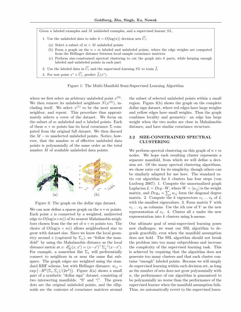
Figure 3: The graph on the dollar sign dataset.

We can now define a sparse graph on the n+m points.Each point x is connected by a weighted, undirectededge to O(log(n+m)) of its nearest Mahalanobis neigh-bors chosen from the the set of n + m points too. Thechoice of O(log(n + m)) allows neighborhood size togrow with dataset size. Since we know the local geom-etry around x (captured by Σx), we “follow the man-ifold” by using the Mahalanobis distance as the localdistance metric at x: d2

M (x, x′) = (x−x′)>Σ−1x (x−x′).

For example, a somewhat flat Σx will preferentiallyconnect to neighbors in or near the same flat sub-space. The graph edges are weighted using the stan-dard RBF scheme, but with Hellinger distance: wij =exp

(−H2(Σi,Σj)/(2σ2)

). Figure 3(a) shows a small

part of a synthetic “dollar sign” dataset, consisting oftwo intersecting manifolds: “S” and “|”. The greendots are the original unlabeled points, and the ellip-soids are the contours of covariance matrices around

the subset of selected unlabeled points within a smallregion. Figure 3(b) shows the graph on the completedollar sign dataset, where red edges have large weightsand yellow edges have small weights. Thus the graphcombines locality and geometry: an edge has largeweight when the two nodes are close in Mahalanobisdistance, and have similar covariance structure.

3.2 SIZE-CONSTRAINED SPECTRALCLUSTERING

We perform spectral clustering on this graph of n+mnodes. We hope each resulting cluster represents aseparate manifold, from which we will define a deci-sion set. Of the many spectral clustering algorithms,we chose ratio cut for its simplicity, though others canbe similarly adapted for use here. The standard ra-tio cut algorithm for k clusters has four steps (vonLuxburg 2007): 1. Compute the unnormalized graphLaplacian L = Deg−W , where W = [wij ] is the weightmatrix, and Degii =

∑j wij form the diagonal degree

matrix. 2. Compute the k eigenvectors v1 . . . vk of Lwith the smallest eigenvalues. 3. Form matrix V withv1 . . . vk as columns. Use the ith row of V as the newrepresentation of xi. 4. Cluster all x under the newrepresentation into k clusters using k-means.

Our ultimate goal of semi-supervised learning posesnew challenges; we want our SSL algorithm to de-grade gracefully, even when the manifold assumptiondoes not hold. The SSL algorithm should not breakthe problem into too many subproblems and increasethe complexity of the supervised learning task. Thisis achieved by requiring that the algorithm does notgenerate too many clusters and that each cluster con-tains “enough” labeled points. Because we will simplydo supervised learning within each decision set, as longas the number of sets does not grow polynomially withn, the performance of our algorithm is guaranteed tobe polynomially no worse than the performance of thesupervised learner when the manifold assumption fails.Thus, we automatically revert to the supervised learn-


ing performance. One way to achieve this is to havethree requirements: i) the number of clusters growsas k ∼ O(log(n)); ii) each cluster must have at leasta ∼ O(n/ log2(n)) labeled points; iii) each spectralcluster must have at least b ∼ O(m/ log2(n)) unla-beled points. The first sets the number of clusters k,allowing more clusters and thus handling more com-plex problems as labeled data size grows, while suffer-ing only a logarithmic performance loss compared toa supervised learner if the manifold assumption fails.The second requirement ensures that each decision sethas O(n) labeled points up to log factor2. The thirdis similar, and makes spectral clustering more robust.

Spectral clustering with minimum size constraints a, bon each cluster is an open problem. Directly en-forcing these constraints in graph partitioning leadsto difficult integer programs. Instead, we enforcethe constraints in k-means (step 4) of spectral clus-tering. Our approach is a straightforward extensionto the constrained k-means algorithm of Bradley etal. (Bradley, Bennett & Demiriz 2000). For point xi,let Ti1 . . . Tik ∈ R be its cluster indicators: ideally,Tih = 1 if xi is in cluster h, and 0 otherwise. Letc1 . . . ck ∈ Rd denote the cluster centers. Constrainedk-means is the iterative minimization over T and c ofthe following problem:

minT,c

∑n+mi=1

∑kh=1 Tih‖xi − ch‖2

s.t.∑k

h=1 Tih = 1, T ≥ 0∑ni=1 Tih ≥ a,

∑n+mi=n+1 Tih ≥ b, h = 1 . . . k, (2)

where we assume the points are ordered so that thefirst n points are labeled. Fixing T , optimizing overc is trivial, and amounts to moving the centers to thecluster means.

Bradley et al. showed that fixing c and optimizing Tcan be converted into a Minimum Cost Flow problem,which can be exactly solved. In a Minimum Cost Flowproblem, there is a directed graph where each node iseither a “supply node” with a number r > 0, or a“demand node” with r < 0. The arcs from i → j isassociated with cost sij , and flow tij . The goal is tofind the flow t such that supply meets demand at allnodes, while the cost is minimized:

mint

∑i→j

sijtij s.t.∑

j

tij −∑

j

tji = ri, ∀i. (3)

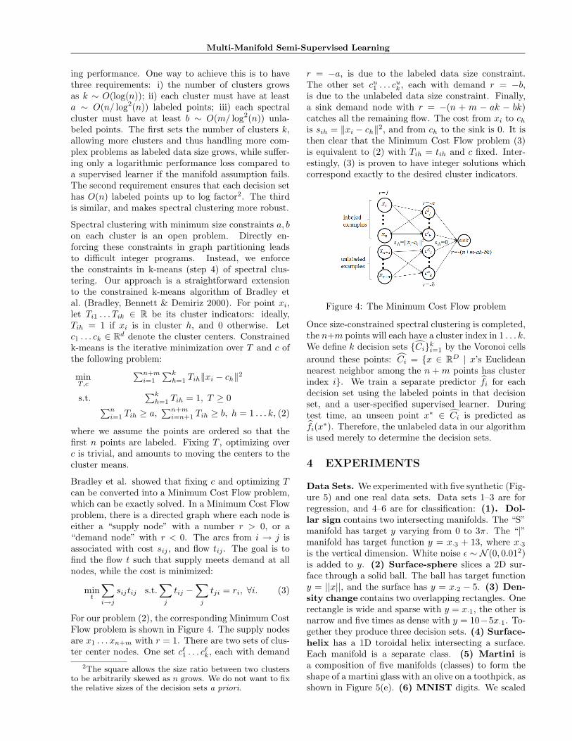
For our problem (2), the corresponding Minimum CostFlow problem is shown in Figure 4. The supply nodesare x1 . . . xn+m with r = 1. There are two sets of clus-ter center nodes. One set c`

1 . . . c`k, each with demand

2The square allows the size ratio between two clustersto be arbitrarily skewed as n grows. We do not want to fixthe relative sizes of the decision sets a priori.

r = −a, is due to the labeled data size constraint.The other set cu

1 . . . cuk , each with demand r = −b,

is due to the unlabeled data size constraint. Finally,a sink demand node with r = −(n + m − ak − bk)catches all the remaining flow. The cost from xi to ch

is sih = ‖xi − ch‖2, and from ch to the sink is 0. It isthen clear that the Minimum Cost Flow problem (3)is equivalent to (2) with Tih = tih and c fixed. Inter-estingly, (3) is proven to have integer solutions whichcorrespond exactly to the desired cluster indicators.

Figure 4: The Minimum Cost Flow problem

Once size-constrained spectral clustering is completed,the n+m points will each have a cluster index in 1 . . . k.We define k decision sets Cik

i=1 by the Voronoi cellsaround these points: Ci = x ∈ RD | x’s Euclideannearest neighbor among the n + m points has clusterindex i. We train a separate predictor fi for eachdecision set using the labeled points in that decisionset, and a user-specified supervised learner. Duringtest time, an unseen point x∗ ∈ Ci is predicted asfi(x∗). Therefore, the unlabeled data in our algorithmis used merely to determine the decision sets.

4 EXPERIMENTS

Data Sets. We experimented with five synthetic (Fig-ure 5) and one real data sets. Data sets 1–3 are forregression, and 4–6 are for classification: (1). Dol-lar sign contains two intersecting manifolds. The “S”manifold has target y varying from 0 to 3π. The “|”manifold has target function y = x·3 + 13, where x·3is the vertical dimension. White noise ε ∼ N (0, 0.012)is added to y. (2) Surface-sphere slices a 2D sur-face through a solid ball. The ball has target functiony = ||x||, and the surface has y = x·2 − 5. (3) Den-sity change contains two overlapping rectangles. Onerectangle is wide and sparse with y = x·1, the other isnarrow and five times as dense with y = 10−5x·1. To-gether they produce three decision sets. (4) Surface-helix has a 1D toroidal helix intersecting a surface.Each manifold is a separate class. (5) Martini isa composition of five manifolds (classes) to form theshape of a martini glass with an olive on a toothpick, asshown in Figure 5(e). (6) MNIST digits. We scaled


0 200 400 6000

5

10

15

20

25

n

MS

E

GlobalSSLClairvoyant

0 200 400 6000

2

4

6

8

10

n

MS

E


0 200 400 6000

5

10

n

MS

E


0 200 400 6000

0.1

0.2

0.3

0.4

0.5

n

Err

or r

ate

GlobalSSL

0 200 400 6000

0.1

0.2

0.3

n

Err

or r

ate

GlobalSSL

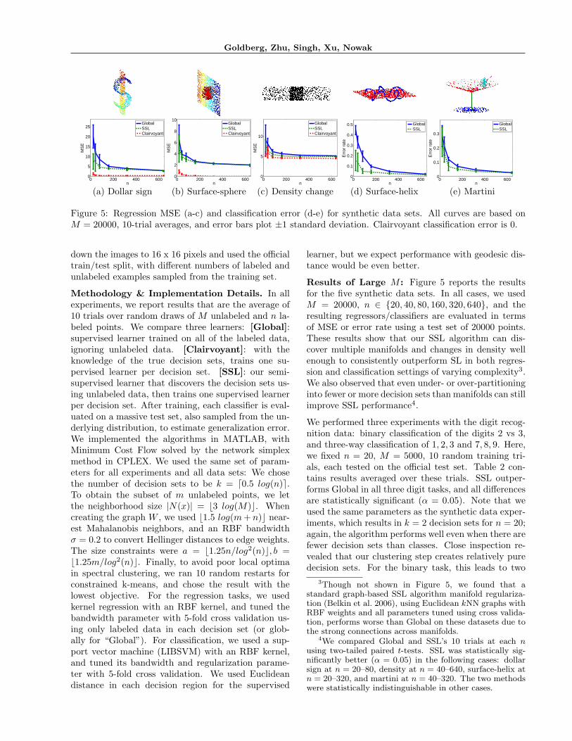
(a) Dollar sign (b) Surface-sphere (c) Density change (d) Surface-helix (e) Martini

Figure 5: Regression MSE (a-c) and classification error (d-e) for synthetic data sets. All curves are based onM = 20000, 10-trial averages, and error bars plot ±1 standard deviation. Clairvoyant classification error is 0.

down the images to 16 x 16 pixels and used the officialtrain/test split, with different numbers of labeled andunlabeled examples sampled from the training set.

Methodology & Implementation Details. In allexperiments, we report results that are the average of10 trials over random draws of M unlabeled and n la-beled points. We compare three learners: [Global]:supervised learner trained on all of the labeled data,ignoring unlabeled data. [Clairvoyant]: with theknowledge of the true decision sets, trains one su-pervised learner per decision set. [SSL]: our semi-supervised learner that discovers the decision sets us-ing unlabeled data, then trains one supervised learnerper decision set. After training, each classifier is eval-uated on a massive test set, also sampled from the un-derlying distribution, to estimate generalization error.We implemented the algorithms in MATLAB, withMinimum Cost Flow solved by the network simplexmethod in CPLEX. We used the same set of param-eters for all experiments and all data sets: We chosethe number of decision sets to be k = d0.5 log(n)e.To obtain the subset of m unlabeled points, we letthe neighborhood size |N(x)| = b3 log(M)c. Whencreating the graph W , we used b1.5 log(m + n)c near-est Mahalanobis neighbors, and an RBF bandwidthσ = 0.2 to convert Hellinger distances to edge weights.The size constraints were a = b1.25n/log2(n)c, b =b1.25m/log2(n)c. Finally, to avoid poor local optimain spectral clustering, we ran 10 random restarts forconstrained k-means, and chose the result with thelowest objective. For the regression tasks, we usedkernel regression with an RBF kernel, and tuned thebandwidth parameter with 5-fold cross validation us-ing only labeled data in each decision set (or glob-ally for “Global”). For classification, we used a sup-port vector machine (LIBSVM) with an RBF kernel,and tuned its bandwidth and regularization parame-ter with 5-fold cross validation. We used Euclideandistance in each decision region for the supervised

learner, but we expect performance with geodesic dis-tance would be even better.

Results of Large M : Figure 5 reports the resultsfor the five synthetic data sets. In all cases, we usedM = 20000, n ∈ 20, 40, 80, 160, 320, 640, and theresulting regressors/classifiers are evaluated in termsof MSE or error rate using a test set of 20000 points.These results show that our SSL algorithm can dis-cover multiple manifolds and changes in density wellenough to consistently outperform SL in both regres-sion and classification settings of varying complexity3.We also observed that even under- or over-partitioninginto fewer or more decision sets than manifolds can stillimprove SSL performance4.

We performed three experiments with the digit recog-nition data: binary classification of the digits 2 vs 3,and three-way classification of 1, 2, 3 and 7, 8, 9. Here,we fixed n = 20, M = 5000, 10 random training tri-als, each tested on the official test set. Table 2 con-tains results averaged over these trials. SSL outper-forms Global in all three digit tasks, and all differencesare statistically significant (α = 0.05). Note that weused the same parameters as the synthetic data exper-iments, which results in k = 2 decision sets for n = 20;again, the algorithm performs well even when there arefewer decision sets than classes. Close inspection re-vealed that our clustering step creates relatively puredecision sets. For the binary task, this leads to two

3Though not shown in Figure 5, we found that astandard graph-based SSL algorithm manifold regulariza-tion (Belkin et al. 2006), using Euclidean kNN graphs withRBF weights and all parameters tuned using cross valida-tion, performs worse than Global on these datasets due tothe strong connections across manifolds.

4We compared Global and SSL’s 10 trials at each nusing two-tailed paired t-tests. SSL was statistically sig-nificantly better (α = 0.05) in the following cases: dollarsign at n = 20–80, density at n = 40–640, surface-helix atn = 20–320, and martini at n = 40–320. The two methodswere statistically indistinguishable in other cases.


Table 2: 10-trial average test set error rates ± onestandard deviation for handwritten digit recognition.

Method 2 vs 3 1, 2, 3 7, 8, 9Global 0.17± 0.12 0.20± 0.10 0.33± 0.20SSL 0.05± 0.01 0.10± 0.04 0.20± 0.10

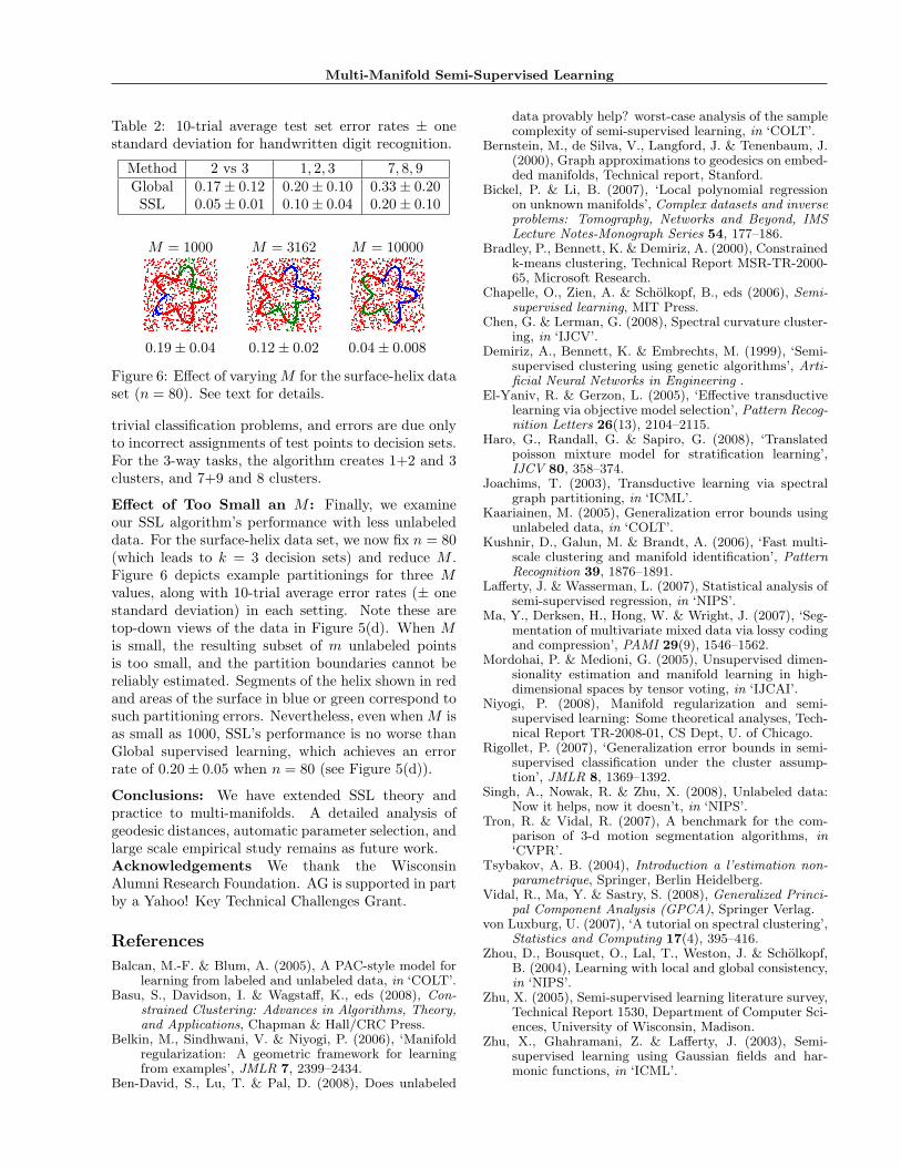
M = 1000 M = 3162 M = 10000

0.19± 0.04 0.12± 0.02 0.04± 0.008

Figure 6: Effect of varying M for the surface-helix dataset (n = 80). See text for details.

trivial classification problems, and errors are due onlyto incorrect assignments of test points to decision sets.For the 3-way tasks, the algorithm creates 1+2 and 3clusters, and 7+9 and 8 clusters.

Effect of Too Small an M : Finally, we examineour SSL algorithm’s performance with less unlabeleddata. For the surface-helix data set, we now fix n = 80(which leads to k = 3 decision sets) and reduce M .Figure 6 depicts example partitionings for three Mvalues, along with 10-trial average error rates (± onestandard deviation) in each setting. Note these aretop-down views of the data in Figure 5(d). When Mis small, the resulting subset of m unlabeled pointsis too small, and the partition boundaries cannot bereliably estimated. Segments of the helix shown in redand areas of the surface in blue or green correspond tosuch partitioning errors. Nevertheless, even when M isas small as 1000, SSL’s performance is no worse thanGlobal supervised learning, which achieves an errorrate of 0.20± 0.05 when n = 80 (see Figure 5(d)).

Conclusions: We have extended SSL theory andpractice to multi-manifolds. A detailed analysis ofgeodesic distances, automatic parameter selection, andlarge scale empirical study remains as future work.Acknowledgements We thank the WisconsinAlumni Research Foundation. AG is supported in partby a Yahoo! Key Technical Challenges Grant.

References

Balcan, M.-F. & Blum, A. (2005), A PAC-style model forlearning from labeled and unlabeled data, in ‘COLT’.

Basu, S., Davidson, I. & Wagstaff, K., eds (2008), Con-strained Clustering: Advances in Algorithms, Theory,and Applications, Chapman & Hall/CRC Press.

Belkin, M., Sindhwani, V. & Niyogi, P. (2006), ‘Manifoldregularization: A geometric framework for learningfrom examples’, JMLR 7, 2399–2434.

Ben-David, S., Lu, T. & Pal, D. (2008), Does unlabeled

data provably help? worst-case analysis of the samplecomplexity of semi-supervised learning, in ‘COLT’.

Bernstein, M., de Silva, V., Langford, J. & Tenenbaum, J.(2000), Graph approximations to geodesics on embed-ded manifolds, Technical report, Stanford.

Bickel, P. & Li, B. (2007), ‘Local polynomial regressionon unknown manifolds’, Complex datasets and inverseproblems: Tomography, Networks and Beyond, IMSLecture Notes-Monograph Series 54, 177–186.

Bradley, P., Bennett, K. & Demiriz, A. (2000), Constrainedk-means clustering, Technical Report MSR-TR-2000-65, Microsoft Research.

Chapelle, O., Zien, A. & Scholkopf, B., eds (2006), Semi-supervised learning, MIT Press.

Chen, G. & Lerman, G. (2008), Spectral curvature cluster-ing, in ‘IJCV’.

Demiriz, A., Bennett, K. & Embrechts, M. (1999), ‘Semi-supervised clustering using genetic algorithms’, Arti-ficial Neural Networks in Engineering .

El-Yaniv, R. & Gerzon, L. (2005), ‘Effective transductivelearning via objective model selection’, Pattern Recog-nition Letters 26(13), 2104–2115.

Haro, G., Randall, G. & Sapiro, G. (2008), ‘Translatedpoisson mixture model for stratification learning’,IJCV 80, 358–374.

Joachims, T. (2003), Transductive learning via spectralgraph partitioning, in ‘ICML’.

Kaariainen, M. (2005), Generalization error bounds usingunlabeled data, in ‘COLT’.

Kushnir, D., Galun, M. & Brandt, A. (2006), ‘Fast multi-scale clustering and manifold identification’, PatternRecognition 39, 1876–1891.

Lafferty, J. & Wasserman, L. (2007), Statistical analysis ofsemi-supervised regression, in ‘NIPS’.

Ma, Y., Derksen, H., Hong, W. & Wright, J. (2007), ‘Seg-mentation of multivariate mixed data via lossy codingand compression’, PAMI 29(9), 1546–1562.

Mordohai, P. & Medioni, G. (2005), Unsupervised dimen-sionality estimation and manifold learning in high-dimensional spaces by tensor voting, in ‘IJCAI’.

Niyogi, P. (2008), Manifold regularization and semi-supervised learning: Some theoretical analyses, Tech-nical Report TR-2008-01, CS Dept, U. of Chicago.

Rigollet, P. (2007), ‘Generalization error bounds in semi-supervised classification under the cluster assump-tion’, JMLR 8, 1369–1392.

Singh, A., Nowak, R. & Zhu, X. (2008), Unlabeled data:Now it helps, now it doesn’t, in ‘NIPS’.

Tron, R. & Vidal, R. (2007), A benchmark for the com-parison of 3-d motion segmentation algorithms, in‘CVPR’.

Tsybakov, A. B. (2004), Introduction a l’estimation non-parametrique, Springer, Berlin Heidelberg.

Vidal, R., Ma, Y. & Sastry, S. (2008), Generalized Princi-pal Component Analysis (GPCA), Springer Verlag.

von Luxburg, U. (2007), ‘A tutorial on spectral clustering’,Statistics and Computing 17(4), 395–416.

Zhou, D., Bousquet, O., Lal, T., Weston, J. & Scholkopf,B. (2004), Learning with local and global consistency,in ‘NIPS’.

Zhu, X. (2005), Semi-supervised learning literature survey,Technical Report 1530, Department of Computer Sci-ences, University of Wisconsin, Madison.

Zhu, X., Ghahramani, Z. & Lafferty, J. (2003), Semi-supervised learning using Gaussian fields and har-monic functions, in ‘ICML’.

Documents

Multi-Manifold Semi-Supervised Learning