ORE Open Research Exeter

TITLE

Multi-Modal Optimisation using a Localised Surrogates Assisted Evolutionary Algorithm

AUTHORS

Fieldsend, Jonathan E.

DEPOSITED IN ORE

17 September 2013

This version available at

http://hdl.handle.net/10871/13542

COPYRIGHT AND REUSE

Open Research Exeter makes this work available in accordance with publisher policies.

A NOTE ON VERSIONS

The version presented here may differ from the published version. If citing, you are advised to consult the published version for pagination, volume/issue and date ofpublication

Multi-Modal Optimisation using a LocalisedSurrogates Assisted Evolutionary Algorithm

Jonathan E. FieldsendComputer Science

University of ExeterExeter, EX4 4QF

Email: J.E.Fieldsend@exeter.ac.uk

Abstract—There has been a steady growth in interest inniching approaches within the evolutionary computation com-munity, as an increasing number of real world problems arediscovered that exhibit multi-modality of varying degrees ofintensity (modes). It is often useful to locate and memorisethe modes encountered – this is because the optimal decisionparameter combinations discovered may not be feasible whenmoving from a mathematical model emulating the real problemto engineering an actual solution, or the model may be in errorin some regions. As such a range of disparate modal solutions isof practical use. This paper investigates the use of a collection oflocalised surrogate models for niche/mode discovery, and analysesthe performance of a novel evolutionary algorithm (EA) whichembeds these surrogates into its search process. Results obtainedare compared to the published performance of state-of-the-artevolutionary algorithms developed for multi-modal problems. Wefind that using a collection of localised surrogates not only makesthe problem tractable from a model-fitting viewpoint, it alsoproduces competitive results with other EA approaches.

I. INTRODUCTION

Optimisation problems in the real world often exhibit adegree of multi-modality, be it only a few modes to contendwith, or potentially a vast number. That is, in a particularvolume of design space there may be more than one solutionwhich performs equally as well as another, but the regionsbetween these solutions map to quality values distinctly lessgood. These are often conceptualised as peaks (or troughs ifthe quality measure is to be minimised) – and are referred toas niches or modes.

Decision makers are often interested in locating disparatepeaks, as they can offer insight into the behaviour of theproblem they are dealing with. Additionally, by discoveringparameter combinations which have the equivalent (or sim-ilar) behaviour, but which are distributed widely in designspace, a wide range of good potential design solutions canbe subsequently assessed. Often the model optimised is asoftware emulation of a physical process, whose mappingmay not be exact in all regions, therefore a spread of goodsolutions is typically a desired output; as realising a particularparameter combination may turn out to be infeasible from amanufacturing point of view, or when manufactured may notbehave as emulated.

Many methods exist to search for multiple optima, withfitness-sharing and crowding [1] being two popular evolu-tionary computation (EC) approaches. Essentially these pro-mote regional subpopulations of a search population, who

are concerned with optimising separate modes. As recentlyhighlighted in [2], these algorithms are often highly parame-terised themselves, and rely on well-chosen values to performas required. Other approaches that have been developed foruse within evolutionary algorithms (EAs) include clustering[3], derating [4], restricted tournament selection [5], speciation[6], and stretching and deflation [7] (to name but a few).

Here we take a different approach to niching, fitting localsurrogate models to regions of the design space, and selectnew design parameters to assess based on the prediction ofthese models. The number of local modes is not predefined,allowing the algorithm to learn the degree of multi-modality asit searches the design space. It accomplishes this by mergingregions covered by surrogates, and by searching in new regionsvia both recombination and speculatively looking in new areas.Results for this localised surrogates assisted evolutionary algo-rithm are presented on a number of multi-modal test functionsfrom the literature [8]–[10].

The paper proceeds as follows. In Section II we providea short description of the general multi-modal optimisationproblem, this is followed by a short overview of surrogate-based optimisation for multi-modal problems and local modelfitting in Section III. In Section IV the multi-modal optimisa-tion algorithm is described, and in Section V its empiricalperformance is compared to that of a number of recentlydeveloped algorithms on a range of standard test problems.The paper concludes with a discussion in Section VI.

II. MULTI-MODAL LANDSCAPES

Many methods have been developed for locating multipleoptima. From the basic ‘Multistart’ approach, which applieslocal search from randomly generated locations [11] – to moresophisticated techniques like fitness sharing and crowding,which both fall in the broader area of niching methods. Holland[12] first introduced the fitness sharing concept, which waslater refined as a means to partition the search population intodifferent subpopulations based on their fitness [13]. A succinctoverview of these general ideas is presented in [1].

The general aim in multi-modal optimisation is similar tothat of global optimisation, that is, without loss of generality,we seek to maximise f(x), where x ∈ X ⊆ RK – thefeasible domain as defined by any equality and inequalityconstraints. In the case of a multi-modal problem, we seeknot simply to discover a single x ∈ X which maximises f(x),but the set {x∗} ∈ X of solutions which obtain the maximum

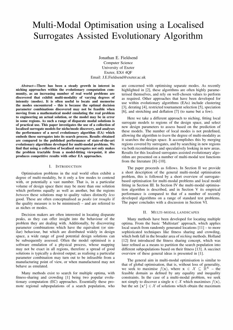
(a) Inverted Vincent function. (b) Composite function 1.

Fig. 1. Example multi-modal function landscapes: (a) has 36 global optima, (b) has a mixture of six global modes and many local modes.

possible function response, but which inhabit isolated peakregions. That is, the mapped objective values in the immediateregion of an x∗ are all lower than f(x∗). Two example multi-modal problems are shown in Figure 1. Figure 1a has anasymmetric distribution of many global optima, Figure 1b hasfewer global optima, but many local optima. Local optima(local modes/peaks) are locations which are surrounded in theimmediate vicinity with less ‘fit’ solutions (lower responsesfrom f(·)), but which do not themselves have the highestpossible fitness.

III. SURROGATE-BASED OPTIMISATION

The use of surrogates within evolutionary optimisationalgorithms has started receiving serious attention in the lastdecade, a good recent overview of area can be found in [14].Many industrial problems are expensive to evaluate, and tomitigate this surrogate models fit a estimate of the cost function(based on previously evaluated design parametrisations, andany prior knowledge available). These can then be used incombination with an EA to guide the search process (althoughreference back to the real fitness function is required in orderto update the surrogate – and to compensate for any falselyinduced maxima). Most areas of research in surrogates areconcerned with the type of surrogate used, and how thesurrogate will be integrated within the search process (the‘model management’ problem [14]).

Some previous studies have used surrogate approachesfor multi-modal problems – in [15] a surrogate is used toeffectively ‘smooth’ the cost landscape as a means to eradicatelocal minima for problems with many local modes and asingle maxima. In [16] local weighted ensembles of surrogatesare used for global optimisation, along with lower orderpolynomial surrogates to also smooth local optima as in [15].In [11] a global surrogate is used in conjunction with a localevolutionary search (which exploited memory for good searchdirections [17]) – although they were concerned with finding aglobal peak, rather than all global peaks. Most recently in [18]a classifier was fitted locally to each offspring in a differentialevolution algorithm, to predict their relative rank order when

solutions previously evaluated in their local neighbourhood hada mixed range of fitnesses.

One drawback of many sophisticated models used assurrogates is that they can often themselves take time tofit the data, and often performance (time to learn) scalespoorly with the number of data points. Where the landscape ishighly muti-modal, it is often highly flexible and parameterisedsurrogates that are required. The use of these becomes rapidlyintractable as the number of data samples rises, as, unlessthe problem being optimised is extremely expensive, the time-cost of regularly fitting the surrogate soon outweighs the timecost of evaluating the actual objective function for medium tolong runs. We attempt to side-step this issue here by using acollection of local surrogates, whose remit is only a very smallregion in X , centred on a particular niche estimate, and aretherefore very cheap to fit in comparison to a global model.This approach is also useful as the maxima from a globallyfitted surrogate may not be as accurate as that induced froma model fitted to just those points sampled in the location ofthe globally estimated maxima (see e.g. [19]). In [20] it is alsoobserved that the global error of a surrogate may not be a goodindication of its local error - and as such local fidelity trackingis used to decide when a global model should be refitted tonew data.

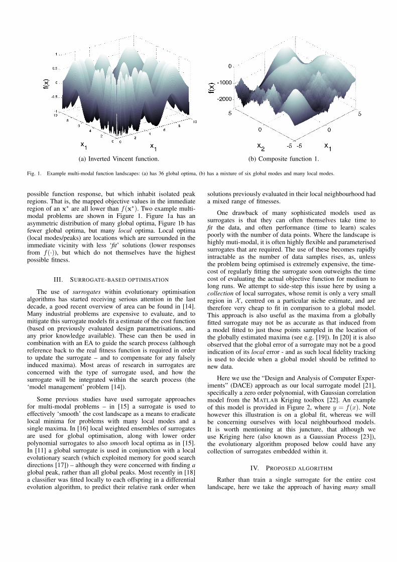
Here we use the “Design and Analysis of Computer Exper-iments” (DACE) approach as our local surrogate model [21],specifically a zero order polynomial, with Gaussian correlationmodel from the MATLAB Kriging toolbox [22]. An exampleof this model is provided in Figure 2, where y = f(x). Notehowever this illustration is on a global fit, whereas we willbe concerning ourselves with local neighbourhood models.It is worth mentioning at this juncture, that although weuse Kriging here (also known as a Gaussian Process [23]),the evolutionary algorithm proposed below could have anycollection of surrogates embedded within it.

IV. PROPOSED ALGORITHM

Rather than train a single surrogate for the entire costlandscape, here we take the approach of having many small

0 0.1 0.2 0.3 0.4 0.5 0.6 0.7 0.8 0.9 1−0.8

−0.6

−0.4

−0.2

0

0.2

0.4

0.6

0.8

1

x

y

0 0.1 0.2 0.3 0.4 0.5 0.6 0.7 0.8 0.9 1−0.4

−0.2

0

0.2

0.4

0.6

0.8

1

1.2

x

y

Fig. 2. Kriging surrogate fitness estimate on the equal maxima test function.Top: based on 10 random samples of x. Bottom: based on 30 random samplesof x. The dashed lines show +/- the root mean squared error estimate providedby the fitted surrogate at each x location.

surrogates, who are concerned only with the local landscapesurrounding the currently estimated niches.

Because we only fit the surrogate to a small volume of X ,we only use previously evaluated solutions in the immediatevicinity to fit the model parameters, thus model fitting at eachgeneration is extremely rapid, even though there may be manysurrogates fitted. Indeed, it is orders of magnitude quickerthan fitting a single model for all the data (as fitting a singlemodel is an O(n3) operation – where n is the number ofdata points used). The algorithm is self-adaptive, with thenumber of niches maintained depending on the propertiesof the landscape discovered, and it seeks to balance bothexploration of the space for previously undiscovered niches,and exploitation of the niches found thus far. As such, thenumber of niches in X does not need to be known a priori,or a vast search population maintained right from the start –instead the number of niches dynamically shrinks or expandsas the search progresses. The algorithm maintains a set of setsof niche histories X, where Xi is the set of m designs {x}mj=1,which are used to define the immediate peak region of the ithniche. Each Xi therefore includes a single x∗ estimate. Yi

is the collection of corresponding responses from f(·) for theelements of Xi.

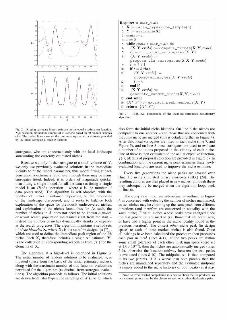
The algorithm at a high-level is described in Figure 3.The initial number of random solutions to be evaluated, n, isinputted (these form the basis of the initial estimated niches),along with the maximum number of true function evaluationspermitted for the algorithm (as distinct from surrogate evalua-tions). The algorithm proceeds as follows. The initial solutionsare drawn from latin hypercube sampling of X (line 1), which

Require: n,max evals1: X := latin_hypercube_sample(n)2: Y := evaluate(X)3: evals := n4: t := 05: while evals < max evals do6: {X,Y, evals} := compare_niches(X,Y, evals)7: S := fit_local_surrogates(X,Y)8: {X,Y, evals} :=

propose_via_surrogates(S,X,Y, evals)9: t := t+ 1

10: if t = 5 then11: {X,Y, evals} :=

crossover_niches(X,Y, evals)12: t := 013: end if14: {X,Y, evals} :=

generate_random_niche(X,Y, evals)15: end while16: {X∗, Y ∗} := extract_peak_members(X,Y)17: return {X∗, Y ∗}

Fig. 3. High-level pseudocode of the localised surrogates evolutionaryalgorithm.

also form the initial niche histories. On line 6 the niches arecompared to one another – and those that are concerned withthe same niche are merged (this is detailed further in Figure 4).After this, local surrogates are fitted to each niche (line 7, andFigure 5), and on line 8 these surrogates are used to evaluatea number of solutions proposed in the vicinity of each niche.One of these is then evaluated on the actual objective function,f(·), (details of proposal selection are provided in Figure 6). Incombination with the current niche peak estimates these newlyevaluated locations are used to improve the niche estimate.

Every five generations the niche peaks are crossed over(line 11) using simulated binary crossover (SBX) [24]. Theresulting children are then placed in new niches (although thesemay subsequently be merged when the algorithm loops backto line 6).

The compare_niches subroutine, as outlined in Figure4, is concerned with reducing the number of niches maintained,as two niches may be climbing up the same peak from differentdirections (and therefore are concerned in actuality with thesame niche). First all niches whose peaks have changed sincethe last generation are marked (i.e. those that are brand new,or have had a higher point in the niche locality found in theprevious iteration). The closest other niche peak (in designspace) to each of these marked niches is also found. Onceall pairings have been calculated the procedure then processeseach pair in turn1 (lines 4-17). If the two peaks are withinsome small tolerance of each other in design space (here setat 1.0×10−3), then the niches are automatically merged (lines5-6), otherwise the location midway between the two peaksis evaluated (lines 8-10). The midpoint, x′, is then comparedto its two parents. If it is worse than both parents then theniches are maintained separately and the evaluated midpointis simply added to the niche histories of both peaks (as it may

1Note, to avoid wasted computation it is best to check the list produced, astwo changed points may be the closest to each other, thus duplicating pairs.

Require: X,Y, evals1: {X∗, Y ∗} := extract_peak_members(X,Y)2: index members in X∗ whose location has moved in the

last generation3: find the closest other niche to each changed niche4: for each selected niche pair X∗i and X∗j do5: if distance(X∗i , X∗j ) ≤ tolerance then6: merge niches7: else8: find the midpoints, x′, for the paired niches9: evaluate midpoint for paired niches, y′ = f(x′)

10: evals := evals+ 111: if y′ < Y ∗i ∧ y′ < Y ∗j then12: add x′ to both Xi and Xj

13: else14: merge niches15: end if16: end if17: end for18: return {X,Y, evals}

Fig. 4. The compare_niches subroutine.

Require: X,Y1: for each niche history set Xi do2: Xi := truncate_least_fit(Xi,Yi, 50)3: k = min(|Xi|, 50)4: if k = 1 then5: fit Si using (up to) 10 closest niche peaks in

parameter space6: else7: fit Si using Xi members8: end if9: end for

10: return SFig. 5. The fit_local_surrogates subroutine.

prove useful to fitting their local surrogates later). However ifit is better than one or both of its parents, then the niches aremerged (and the mid point added to the history of the resultantmerged niche, and becomes its x∗ estimate if appropriate).

In the fit_local_surrogates subroutine (Figure 5)the niche history stored for each niche is used to fit a surrogatein the region of the peak estimate. A maximum of 50 locationsare stored in each peak’s niche history. When the numberexceeds 50, the least fit are truncated (line 2) – note, thisdistance is calculated from f(x∗) rather than x∗. If there isonly one element in the current niche, then the 10 closest otherpeaks in search space (or fewer if there are fewer than 10niches in total), are used to fit the surrogate model (lines 4-5).

Following the fitting of the surrogate models, the surrogatesare then used to evaluate proposed solutions drawn in theimmediate vicinity of the niche peak, as described in Figure 6.In the special case where adjacent niches have been used to fitthe surrogate, due to the niche not currently having a historyof its own, then a hypersphere in X is placed around the nichepeak. The hypersphere width is determined by the distance tothe closest next niche peak (in design space), otherwise thediameter of the hypersphere placed around the peak is chosen

Require: S,X,Y, evals1: for each fitted surrogate Xi do2: k = min(|Xi|, 10)3: if k = 1 then4: get parameter space distance d to closest other niche

peak5: else6: u := U(0, 1)7: if u < 1

3 then8: get parameter space distance d to the closest

niche history member (by fitness)9: else if u < 2

3 then10: get parameter space distance d to the kth closest

niche history member (by fitness)11: else12: get parameter space distance d to closest other

niche peak13: end if14: end if15: u := U(0, 1)16: if u < 1

2 then17: generate 100 samples in a truncated Gaussian hy-

persphere, centred on the ith peak, with the hyper-sphere radius set to d/2

18: induce fitness estimate of samples through Si19: select sample x with best predicted fitness20: else21: generate a sample x in a truncated Gaussian hy-

persphere, centred on the ith peak, with the hyper-sphere radius set to d/2

22: end if23: evaluate x on actual problem, to obtain y24: evals := evals+ 125: {X,Y} :=

update_niche(X,Y, i,x, y)26: end for27: return {X,Y, evals}

Fig. 6. The propose_via_surrogates subroutine.

either as the distance to the next fittest point in the niche history(line 8), the distance to the 10th closest point in niche history(line 10) or the distance to the closest next niche peak (line 12).By varying the value chosen for the diameter d in these fashionwe seek to generate putative solutions which are compactlydistributed about the current peak estimate for fine-tuning,and also more widely spread to make larger movements, butalways within the region defined by the current niche andconstrained by the next closest one. Within the hypersphereitself an isotropic Gaussian distribution is used to generate thesamples (the hypersphere radius effectively defining the scalingand truncation point of the Gaussian – with three standarddeviations from the hypersphere centre to its edge). 50% ofthe time 100 samples are drawn from this hypersphere andevaluated by the local surrogate, with the predicted fittest ofthese selected to be evaluated on the actual problem. The other50% of the time we take a single random sample from thetruncated Gaussian and do not fit a surrogate. By choosing thepredicted fittest we are exploiting the estimated peak from thesurrogate, whereas the random selection promotes search inthe neighbourhood of the peak estimate.

Require: X,Y, i,x, y1: {x∗, y∗} := get_peak(Xi,Yi)2: if y > y∗ then3: replace peak with x4: end if5: update niche history with x and y6: return {X,Y}

Fig. 7. The update_niche subroutine.

Require: X,Y, evals1: {X∗, Y ∗} := extract_peak_members(X,Y)2: randomly permute the indices of the peak sets, and hold

in I3: while |I| > 1 do4: remove the last two values held in I , i and j5: crossover X∗i and X∗j to create x′ and x′′

6: evaluate the offspring, x′ and x′′

7: create a new niche for each of the offspring8: evals := evals+ 29: end while

10: return {X,Y, evals}

Fig. 8. The crossover_niches subroutine.

Before returning, the propose_via_surrogates sub-routine passes each of the evaluated proposals to theupdate_niche subroutine, which ascertains whether thenew solution has improved the peak estimate, and is describedin Figure 7. If the new location is worse than the current peak,then the proposal is still added to the history of the currentniche.

The main exploration driver occurs via niche crossover, asdescribed in Figure 8 (the SBX parameter was set to 20 inour empirical work), with additional speculative search via arandom element in each generation (line 14 of Figure 3).

The surrogates provide the main exploitation driver in thealgorithm and crossover the principal exploration mechanism(although there is localised mutation around the peaks asdescribed in Figure 6). Note, the algorithm does not concernitself with how fit the niches it maintains are in relation toeach other – it is only concerned that the niches are locallyfit with respect to the the immediate vicinity around a nichepeak. As such this algorithm will successfully find many peaksof varying heights.

V. EMPIRICAL RESULTS

The algorithm’s performance is compared against the pub-lished results of a number of particle swarm optimisation(PSO) and differential evolution (DE) algorithms previouslyapplied to multi-modal problems. Namely Constricted PSO(CPSO) [25], Gaussian PSO (GPSO) [26], Cauchy and Gaus-sian PSO (CGPSO) [2], DE/rand/1/bin [27] (labelled DE in thetables) and the crowding DE/nrand/1/bin [28] (labelled CDEin the tables). These results are taken from [2] and [29] – andthe form of assessment follows the practice of these articles.

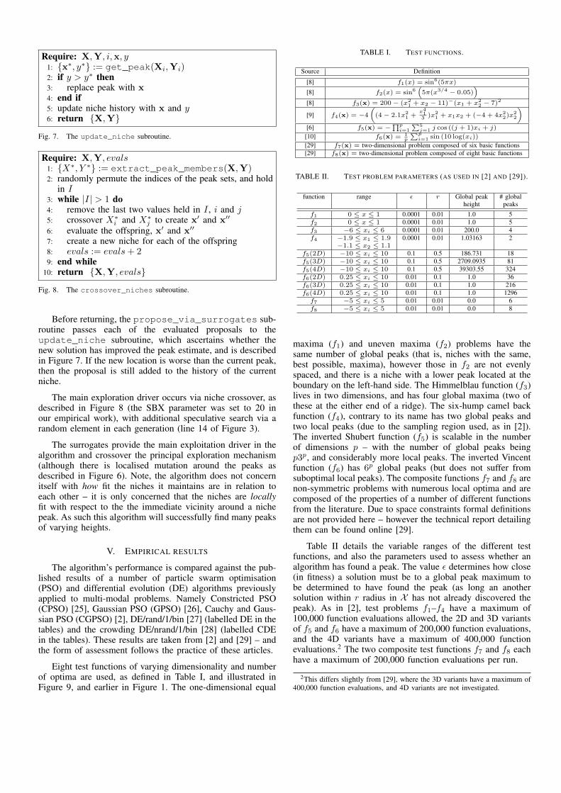
Eight test functions of varying dimensionality and numberof optima are used, as defined in Table I, and illustrated inFigure 9, and earlier in Figure 1. The one-dimensional equal

TABLE I. TEST FUNCTIONS.

Source Definition

[8] f1(x) = sin6(5πx)

[8] f2(x) = sin6(5π(x3/4 − 0.05)

)[8] f3(x) = 200− (x2

1 + x2 − 11)−(x1 + x22 − 7)2

[9] f4(x) = −4((4− 2.1x2

1 +x413 )x2

1 + x1x2 + (−4 + 4x22)x

22

)[6] f5(x) = −

∏pi=1

∑5j=1 j cos ((j + 1)xi + j)

[10] f6(x) = 1p

∑pi=1 sin (10 log(xi))

[29] f7(x) = two-dimensional problem composed of six basic functions[29] f8(x) = two-dimensional problem composed of eight basic functions

TABLE II. TEST PROBLEM PARAMETERS (AS USED IN [2] AND [29]).

function range ε r Global peak # globalheight peaks

f1 0 ≤ x ≤ 1 0.0001 0.01 1.0 5f2 0 ≤ x ≤ 1 0.0001 0.01 1.0 5f3 −6 ≤ xi ≤ 6 0.0001 0.01 200.0 4f4 −1.9 ≤ x1 ≤ 1.9 0.0001 0.01 1.03163 2

−1.1 ≤ x2 ≤ 1.1f5(2D) −10 ≤ xi ≤ 10 0.1 0.5 186.731 18f5(3D) −10 ≤ xi ≤ 10 0.1 0.5 2709.0935 81f5(4D) −10 ≤ xi ≤ 10 0.1 0.5 39303.55 324f6(2D) 0.25 ≤ xi ≤ 10 0.01 0.1 1.0 36f6(3D) 0.25 ≤ xi ≤ 10 0.01 0.1 1.0 216f6(4D) 0.25 ≤ xi ≤ 10 0.01 0.1 1.0 1296f7 −5 ≤ xi ≤ 5 0.01 0.01 0.0 6f8 −5 ≤ xi ≤ 5 0.01 0.01 0.0 8

maxima (f1) and uneven maxima (f2) problems have thesame number of global peaks (that is, niches with the same,best possible, maxima), however those in f2 are not evenlyspaced, and there is a niche with a lower peak located at theboundary on the left-hand side. The Himmelblau function (f3)lives in two dimensions, and has four global maxima (two ofthese at the either end of a ridge). The six-hump camel backfunction (f4), contrary to its name has two global peaks andtwo local peaks (due to the sampling region used, as in [2]).The inverted Shubert function (f5) is scalable in the numberof dimensions p – with the number of global peaks beingp3p, and considerably more local peaks. The inverted Vincentfunction (f6) has 6p global peaks (but does not suffer fromsuboptimal local peaks). The composite functions f7 and f8 arenon-symmetric problems with numerous local optima and arecomposed of the properties of a number of different functionsfrom the literature. Due to space constraints formal definitionsare not provided here – however the technical report detailingthem can be found online [29].

Table II details the variable ranges of the different testfunctions, and also the parameters used to assess whether analgorithm has found a peak. The value ε determines how close(in fitness) a solution must be to a global peak maximum tobe determined to have found the peak (as long an anothersolution within r radius in X has not already discovered thepeak). As in [2], test problems f1–f4 have a maximum of100,000 function evaluations allowed, the 2D and 3D variantsof f5 and f6 have a maximum of 200,000 function evaluations,and the 4D variants have a maximum of 400,000 functionevaluations.2 The two composite test functions f7 and f8 eachhave a maximum of 200,000 function evaluations per run.

2This differs slightly from [29], where the 3D variants have a maximum of400,000 function evaluations, and 4D variants are not investigated.

Equal maxima Uneven maxima

0 0.1 0.2 0.3 0.4 0.5 0.6 0.7 0.8 0.9 10

0.1

0.2

0.3

0.4

0.5

0.6

0.7

0.8

0.9

1

x

y

0 0.1 0.2 0.3 0.4 0.5 0.6 0.7 0.8 0.9 10

0.1

0.2

0.3

0.4

0.5

0.6

0.7

0.8

0.9

1

y

x

Himmelblau Six-hump camel back

x2

x1

−6 −4 −2 0 2 4 6−6

−4

−2

0

2

4

6

x2

x1

−1.5 −1 −0.5 0 0.5 1 1.5

−1

−0.5

0

0.5

1

Inverted Shubert function Composite function 2

x1

x2

−10 −5 0 5 10−10

−5

0

5

10

x1

x2

−5 0 5−5

0

5

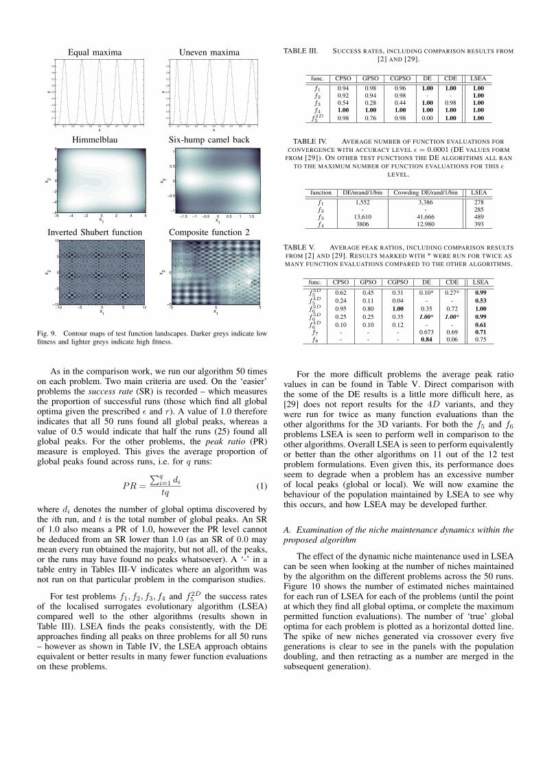
Fig. 9. Contour maps of test function landscapes. Darker greys indicate lowfitness and lighter greys indicate high fitness.

As in the comparison work, we run our algorithm 50 timeson each problem. Two main criteria are used. On the ‘easier’problems the success rate (SR) is recorded – which measuresthe proportion of successful runs (those which find all globaloptima given the prescribed ε and r). A value of 1.0 thereforeindicates that all 50 runs found all global peaks, whereas avalue of 0.5 would indicate that half the runs (25) found allglobal peaks. For the other problems, the peak ratio (PR)measure is employed. This gives the average proportion ofglobal peaks found across runs, i.e. for q runs:

PR =

∑qi=1 ditq

(1)

where di denotes the number of global optima discovered bythe ith run, and t is the total number of global peaks. An SRof 1.0 also means a PR of 1.0, however the PR level cannotbe deduced from an SR lower than 1.0 (as an SR of 0.0 maymean every run obtained the majority, but not all, of the peaks,or the runs may have found no peaks whatsoever). A ‘-’ in atable entry in Tables III-V indicates where an algorithm wasnot run on that particular problem in the comparison studies.

For test problems f1, f2, f3, f4 and f2D5 the success ratesof the localised surrogates evolutionary algorithm (LSEA)compared well to the other algorithms (results shown inTable III). LSEA finds the peaks consistently, with the DEapproaches finding all peaks on three problems for all 50 runs– however as shown in Table IV, the LSEA approach obtainsequivalent or better results in many fewer function evaluationson these problems.

TABLE III. SUCCESS RATES, INCLUDING COMPARISON RESULTS FROM[2] AND [29].

func. CPSO GPSO CGPSO DE CDE LSEA

f1 0.94 0.98 0.96 1.00 1.00 1.00f2 0.92 0.94 0.98 - - 1.00f3 0.54 0.28 0.44 1.00 0.98 1.00f4 1.00 1.00 1.00 1.00 1.00 1.00f2D5 0.98 0.76 0.98 0.00 1.00 1.00

TABLE IV. AVERAGE NUMBER OF FUNCTION EVALUATIONS FORCONVERGENCE WITH ACCURACY LEVEL ε = 0.0001 (DE VALUES FORM

FROM [29]). ON OTHER TEST FUNCTIONS THE DE ALGORITHMS ALL RANTO THE MAXIMUM NUMBER OF FUNCTION EVALUATIONS FOR THIS ε

LEVEL.

function DE/nrand/1/bin Crowding DE/rand/1/bin LSEA

f1 1,552 3,386 278f2 - - 285f3 13,610 41,666 489f4 3806 12,980 393

TABLE V. AVERAGE PEAK RATIOS, INCLUDING COMPARISON RESULTSFROM [2] AND [29]. RESULTS MARKED WITH * WERE RUN FOR TWICE ASMANY FUNCTION EVALUATIONS COMPARED TO THE OTHER ALGORITHMS.

func. CPSO GPSO CGPSO DE CDE LSEA

f3D5 0.62 0.45 0.31 0.10* 0.27* 0.99f4D5 0.24 0.11 0.04 - - 0.53f2D6 0.95 0.80 1.00 0.35 0.72 1.00f3D6 0.25 0.25 0.35 1.00* 1.00* 0.99f4D6 0.10 0.10 0.12 - - 0.61f7 - - - 0.673 0.69 0.71f8 - - - 0.84 0.06 0.75

For the more difficult problems the average peak ratiovalues in can be found in Table V. Direct comparison withthe some of the DE results is a little more difficult here, as[29] does not report results for the 4D variants, and theywere run for twice as many function evaluations than theother algorithms for the 3D variants. For both the f5 and f6problems LSEA is seen to perform well in comparison to theother algorithms. Overall LSEA is seen to perform equivalentlyor better than the other algorithms on 11 out of the 12 testproblem formulations. Even given this, its performance doesseem to degrade when a problem has an excessive numberof local peaks (global or local). We will now examine thebehaviour of the population maintained by LSEA to see whythis occurs, and how LSEA may be developed further.

A. Examination of the niche maintenance dynamics within theproposed algorithm

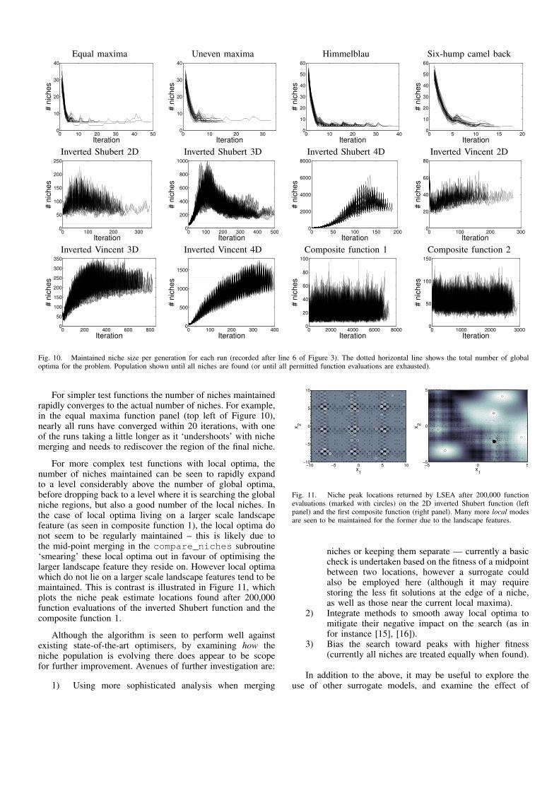
The effect of the dynamic niche maintenance used in LSEAcan be seen when looking at the number of niches maintainedby the algorithm on the different problems across the 50 runs.Figure 10 shows the number of estimated niches maintainedfor each run of LSEA for each of the problems (until the pointat which they find all global optima, or complete the maximumpermitted function evaluations). The number of ‘true’ globaloptima for each problem is plotted as a horizontal dotted line.The spike of new niches generated via crossover every fivegenerations is clear to see in the panels with the populationdoubling, and then retracting as a number are merged in thesubsequent generation).

Equal maxima Uneven maxima Himmelblau Six-hump camel back

0 10 20 30 40 500

10

20

30

40

Iteration

# n

iches

0 10 20 300

10

20

30

40

Iteration

# n

iches

0 10 20 30 400

10

20

30

40

50

60

Iteration

# n

iches

0 5 10 15 200

10

20

30

40

50

60

Iteration

# n

iches

Inverted Shubert 2D Inverted Shubert 3D Inverted Shubert 4D Inverted Vincent 2D

0 100 200 3000

50

100

150

200

250

Iteration

# n

iches

0 100 200 300 400 5000

200

400

600

800

1000

Iteration

# n

iches

0 50 100 150 2000

2000

4000

6000

8000

Iteration

# n

iches

0 100 200 3000

20

40

60

80

Iteration

# n

iches

Inverted Vincent 3D Inverted Vincent 4D Composite function 1 Composite function 2

0 200 400 600 8000

50

100

150

200

250

300

350

Iteration

# n

iches

0 100 200 300 4000

500

1000

1500

Iteration

# n

iches

0 2000 4000 6000 80000

20

40

60

80

100

Iteration

# n

iches

0 1000 2000 30000

50

100

150

Iteration

# n

iches

Fig. 10. Maintained niche size per generation for each run (recorded after line 6 of Figure 3). The dotted horizontal line shows the total number of globaloptima for the problem. Population shown until all niches are found (or until all permitted function evaluations are exhausted).

For simpler test functions the number of niches maintainedrapidly converges to the actual number of niches. For example,in the equal maxima function panel (top left of Figure 10),nearly all runs have converged within 20 iterations, with oneof the runs taking a little longer as it ‘undershoots’ with nichemerging and needs to rediscover the region of the final niche.

For more complex test functions with local optima, thenumber of niches maintained can be seen to rapidly expandto a level considerably above the number of global optima,before dropping back to a level where it is searching the globalniche regions, but also a good number of the local niches. Inthe case of local optima living on a larger scale landscapefeature (as seen in composite function 1), the local optima donot seem to be regularly maintained – this is likely due tothe mid-point merging in the compare_niches subroutine‘smearing’ these local optima out in favour of optimising thelarger landscape feature they reside on. However local optimawhich do not lie on a larger scale landscape features tend to bemaintained. This is contrast is illustrated in Figure 11, whichplots the niche peak estimate locations found after 200,000function evaluations of the inverted Shubert function and thecomposite function 1.

Although the algorithm is seen to perform well againstexisting state-of-the-art optimisers, by examining how theniche population is evolving there does appear to be scopefor further improvement. Avenues of further investigation are:

1) Using more sophisticated analysis when merging

x1

x2

−10 −5 0 5 10−10

−5

0

5

10

x1

x2

−5 0 5−5

0

5

Fig. 11. Niche peak locations returned by LSEA after 200,000 functionevaluations (marked with circles) on the 2D inverted Shubert function (leftpanel) and the first composite function (right panel). Many more local modesare seen to be maintained for the former due to the landscape features.

niches or keeping them separate — currently a basiccheck is undertaken based on the fitness of a midpointbetween two locations, however a surrogate couldalso be employed here (although it may requirestoring the less fit solutions at the edge of a niche,as well as those near the current local maxima).

2) Integrate methods to smooth away local optima tomitigate their negative impact on the search (as infor instance [15], [16]).

3) Bias the search toward peaks with higher fitness(currently all niches are treated equally when found).

In addition to the above, it may be useful to explore theuse of other surrogate models, and examine the effect of

the tolerance value used for merging niches. Also there is apotential to develop a heuristic for convergence checking on aparticular niche (i.e., exploring when to stop evolving a nicheif it is thought the best value in that local region has now beenattained).

Finally, the use of many local surrogates rather than a singleglobal surrogate has large efficiency gains in model fitting,as well as fidelity, however there is still a cost overhead inevaluating proposals with a surrogate. So, for cheap to computef(·) there may be a trade-off in the number of surrogateevaluations to use per iteration when compared to the numberof evaluations of f(·) taken.

VI. DISCUSSION

A new approach to multi-modal optimisation based onusing an EA with a dynamically varying number of localisedsurrogates has been proposed, and evaluated on a range ofproblems. It may be viewed as a sophisticated distributed hill-climber, albeit one employing a degree of communication be-tween immediately adjacent hills, which uses local surrogatesto guide the hill traversal. The EA component is principallyconcerned with searching for new hills to climb, although itwill also exploit any symmetry in the landscape. It is howeverseen to perform well on problems which are non-symmetrictoo.

Analysis of its behaviour indicates there are areas thatcan still be improved, with efficiency gains still to be hadby improving its niche maintenance subroutines, and how ithandles problems with very many local optima. Nevertheless,even in its current form LSEA is found to be competitive withthe state-of-the-art.

ACKNOWLEDGMENTS

The author would like to thank Xiaodong Li for inspiringhim to consider the multi-modal optimisation area anew, andkindly discussing the state of research in the field during theIEEE WCCI 2010 conference. Thanks also to the anonymousreferees for their valuable comments and helpful suggestions.

REFERENCES

[1] B. Sareni and L. Krahenbuhl, “Fitness sharing and niching methodsrevisited,” IEEE Transactions on Evolutionary Computation, vol. 2,no. 3, pp. 97–106, 1998.

[2] X. Li and K. Deb, “Comparing lbest PSO niching algorithms usingdifferent position update rules,” in IEEE Congress on EvolutionaryComputation, 2010, pp. 1564–1571.

[3] X. Yin and N. Germany, “A fast genetic algorithm with sharing schemeusing cluster analysis methods in multi-modal function optimization,”in International Conference on Artificial Neural Networks and GeneticAlgorithms, 1993, pp. 450–457.

[4] D. Beasley, D. R. Bull, and R. Martin, “A sequential niche technique formultimodal function optimization,” Evolutionary Computation, vol. 1,no. 2, pp. 101–125, 1993.

[5] G. Harik, “Finding multimodal solutions using restricted tournamentselection,” in Proceedings of the Sixth International Conference onGenetic Algorithms, 1995, pp. 24–31.

[6] J.-P. Li, M. Balazs, G. Parks, and P. Clarkson, “A species conservinggenetic algorithm for multimodal function optimisation,” EvolutionaryComputation, vol. 10, no. 2, pp. 207–234, 2002.

[7] K. Parsopoulos and M. Vrahatis, “On the computation of all globalminimizers through particle swarm optimization,” IEEE Transactionson Evolutionary Computation, vol. 8, no. 3, pp. 211–224, 2004.

[8] K. Deb, “Genetic algorithms in multimodal function optimization,”Masters thesis and TCGA report no. 89002, Tuscaloosa: University ofAlabama, The Clearinghouse for Genetic Algorithms, Tech. Rep., 1989.

[9] Z. Michalewicz, Genetic Algorithms + Data Structures = EvolutionPrograms. Springer-Verlag, 1996.

[10] O. Shir and T. Back, “Niche radius adaptation in the CMS-ES nichingalgorithm,” in Parallel Problem Solving from Nature - PPSN IX, ser.LNCS, vol. 4193. Springer, 2006, pp. 142–151.

[11] K.-H. Liang, X. Yao, and C. Newton, “Evolutionary Search ofApproximated N-Dimensional Landscapes,” International Journal ofKnowledge-Based Intelligent Engineering Systems, vol. 4, no. 3, pp.172–183, 2000.

[12] J. Holland, Adaptation in Natural and Artificial Systems. Universityof Michigan Press, 1975.

[13] D. E. Goldberg and J. Richardson, “Genetic algorithms with sharingfor multimodal function optimisation,” in Proceedings of the SecondInternational Conference on Genetic Algorithms and their Application.L. Erlbaum Associates Inc., 1987, pp. 41–49.

[14] Y. Jin, “Surrogate-assisted evolutionary computation: Recent advancesand future challenges,” Swarm and Evolutionary Computation, vol. 1,no. 2, pp. 61–70, 2011.

[15] D. Yang and S. J. Flockton, “Evolutionary Algorithms with a Coarse-to-Fine Function Smoothing,” in IEEE International Conference onEvolutionary Computation. IEEE Press, 1995, pp. 657–662.

[16] D. Lim, Y. Jin, Y.-S. Ong, and B. Sendhoff, “Generalizing Surrogate-Assisted Evolutionary Computation,” IEEE Transactions on Evolution-ary Computation, vol. 14, no. 3, pp. 329–355, 2010.

[17] H.-M. Voight and J. M. Lange, “Local Evolutionary Search by Ran-dom Memorizing,” in IEEE International Conference on EvolutionaryComputation. IEEE Press, 1998, pp. 547–552.

[18] X. Lu, K. Tang, and X. Yao, “Classification-assisted Differential Evo-lution for computationally expensive problems,” in IEEE Congress onEvolutionary Computation, 2011, pp. 1986–1993.

[19] Y. Tenne and S. W. Armfield, “A framework for memetic optimizationusing variable global and local surrogate models,” Soft Computing,vol. 13, pp. 781–793, 2009.

[20] Y. Jin, M. Olhofer, and B. Sendhoff, “A framework for evolutionaryoptimization with approximate fitness functions,” IEEE Transactionson Evolutionary Computation, vol. 6, no. 5, pp. 481–494, 2002.

[21] J. Sacks, W. J. Welch, T. J. Mitchell, and H. P. Wynn, “Design andanalysis of computer experiments,” Statistical Science, vol. 4, no. 4,pp. 409–435, 1989.

[22] S. N. Lophaven, H. B. Nielsen, and J. Søndergaard, “DACE A MatlabKriging Toolbox,” Technical Report IMM-TR-2002-12, Informatics andMathematical Modelling, Technical University of Denmark, Tech. Rep.,2002.

[23] C. Rasmussen and C. Williams, Gaussian Processes for MachineLearning. MIT Press, 2006.

[24] K. Deb and R. B. Agrawal, “Simulated Binary Crossover for ContinuosSearch Space,” Department of Mechanical Engineering, Indian Instituteof Technology, Kanpur, IITK/ME/SMD-94027, Tech. Rep., 1994.

[25] M. Clerc and J. Kennedy, “The particle swarm - explosion, stability, andconvergence in a multidimensional complex space,” IEEE Transactionson Evolutionary Computation, vol. 6, pp. 58–73, 2002.

[26] B. Secrest and G. Lamont, “Visualizing particle swarm optimization -gaussian particle swarm optimization,” in Proceedings of the 2003 IEEESwarm Intelligence Symposium, 2003, pp. 198–204.

[27] R. Thomsen, “Multimodal optimization using crowding-based differen-tial evolution,” in IEEE Congress on Evolutionary Computation, 2004,pp. 1382–1389.

[28] M. Epitropakis, V. Plagianakos, and M. Vrahatis, “Finding multipleglobal optima exploiting differential evolution’s niching capability,” inIEEE Symposium on Differential Evolution (IEEE Symposium Series onComputational Intelligence), 2011, pp. 80–87.

[29] X. Li, A. Engelbrecht, and M. Epitropakis, “Benchmark Functionsfor CEC’2013 Special Session and Competition on Niching Methodsfor Multimodal Function Optimization,” Evolutionary Computation andMachine Learning Group, RMIT University, Tech. Rep., 2013.