Embed Size (px)
Citation preview
Multi-model approaches to three-axis missile autopilotdesign under aerodynamic roll angle uncertaintyD-Y Won1*, M-J Tahk1, Y-H Kim2, and H J Kim3
1Korea Advanced Institute of Science and Technology, Daejeon, Republic of Korea2LIG Nex1 Co., Daejeon, Republic of Korea3School of Mechanical and Aerospace Engineering, Seoul National University, Seoul, Republic of Korea
The manuscript was received on 25 February 2011 and was accepted after revision for publication on 12 July 2011.
DOI: 10.1177/0954410011418751
Abstract: The problem of designing a robust three-axis missile autopilot that operates underaerodynamic roll angle uncertainty is addressed in this article. A finite number of local state-space models over an aerodynamic roll angle envelope are developed as a multi-model to rep-resent uncertainty bounds. Two design methods with multi-objective output-feedback controlare proposed. In the first approach, a classical three-loop autopilot structure is slightly modifiedfor the multivariable autopilot design. The optimal gains in the autopilot structure are automat-ically obtained by using a co-evolutionary optimization method that addresses competing spe-cifications and constraints. In the second approach, the mixed H2/H1 performance criteria areguaranteed by multi-objective control synthesis via optimization techniques. Both designapproaches are used in non-linear simulations with variations in the aerodynamic roll angle toprovide satisfactory performance as a three-axis missile autopilot.
Keywords: robust control, three-axis missile autopilot, multi-model approach
1 INTRODUCTION
The increased demand for highly manoeuvrable
modern missiles requires an excellent autopilot
mechanism over a large flight envelope. This requires
the control objectives to be expressed in terms of the
time and frequency domains that should be achieved
in more severe environments, such as those with
undesirable induced roll moments. This increased
complexity, in addition to the expanded capabilities
of a high-performance missile, has been considered
in the autopilot design problem [1, 2]. In classical
approaches, which separately design for the roll,
pitch, and yaw axis and ignore cross-coupling effects,
the influence of high-angle-of-attack aerodynamic
phenomena on stability characteristics is significant.
For instance, the performance of separate controllers
has been limited in some flight boundaries, wherein
the interaction between each of the channels was
minimal.
Over the course of the past decade, there have been
many developments in the field of missile autopilot
design, ranging from classical to modern control
approaches. Both the approximate feedback lineari-
zation and the asymptotic output tracking methods
have been investigated and compared to classical reg-
ulators [3]. Various robust design methods have been
proposed using H1 control or linear parameter-vary-
ing control until recently [4–8]. An adaptive control
design technique has been applied in combination
with non-linear control [9], neural networks control
[10, 11], and sliding mode control approaches [12].
In addition, evolutionary algorithms have also
been used to automatically obtain gains for specific
autopilot configurations [13, 14]. Although these
approaches demonstrate improvements that involve
a fraction of the flight envelope and provide useful
*Corresponding author: Department of Aerospace Engineering,
Korea Advanced Institute of Science and Technology, Daejeon,
305-701, Republic of Korea.
email: [email protected]
1
Proc. IMechE Vol. 000 Part G: J. Aerospace Engineering
at Seoul National University on August 10, 2015pig.sagepub.comDownloaded from
ways to address major design problems, a single con-
troller will not satisfy both the performance and
robustness requirements for an agile missile that
has rapidly changing non-linear dynamics.
On the other hand, studies have been performed to
analyse the non-linearities and cross-coupling with
the controller design in a coupled manner. These
studies have attempted to address the robustness
problem using H1 control technique [15–17], a two-
cascaded structure with an integral action [18], and
feedback linearization technique that is based on
two-time scale separation [19]. These multivariable
robust control techniques can cover a larger flight
envelope and offer a reasonable treatment of the
fully coupled dynamics. However, agile missile auto-
pilot designs have been achieved based on the
assumption that the aerodynamic roll angle can be
precisely estimated. From a practical point of view,
because the angle of attack and the sideslip angle are
not available from direct measurements, it is not triv-
ial to design a highly precise state observer that is
subject to three-axis accelerations or agile manoeu-
vres. For such cases, due to the effects of cross-cou-
pling and the necessity output differentiation, some
assumptions that have been made in the observer
design are not always feasible.
To address these problems, two different three-axis
autopilot design techniques are proposed for the
development of an agile missile controller. The first
design is based on the classical output-feedback con-
trol approach. A conventional three-loop autopilot
configuration is slightly modified with a cross-feed
loop so as to compensate for the cross-coupling
effects that are induced from the variations in the
aerodynamic roll angle. The optimal gains are auto-
matically obtained by using a co-evolutionary opti-
mization that can manage competing specifications
and constraints. The other design uses a mixed H2/
H1 output-feedback control approach. Because high-
angle-of-attack aerodynamics are highly non-linear
and very imprecise, a mix of the H2 and H1 criteria
is selected to guarantee the performance of the three-
axis missile autopilot. An upper bound of the subop-
timal H2 and H1 performance is obtained by linear
matrix inequality (LMI) conditions. In both autopilot
design methods, a multi-model approach is used to
avoid the need for the estimation of the aerodynamic
roll angle. The contribution of the paper can be sum-
marized as follows.
1. The three-axis missile autopilot design using evo-
lutionary and LMI optimization techniques, which
enhances robust performance against cross-cou-
pling effects over a flight envelope, has been
developed.
2. To account for model uncertainties, a finite set of
possible linear time invariant (LTI) models at fixed
operating conditions is considered instead of a
single nominal LTI model. This formulates a prob-
lem of robust control design instead of a problem
of estimating the aerodynamic roll angle. The
application of the multi-model approach to
three-axis missile autopilot design is almost unex-
plored in the literature.
3. A qualitative comparison between two autopilot
design approaches is described as guidelines for
evaluating the potential of each design approach
in terms of its performance, robustness, and
complexity.
Conventional approaches in modern robust con-
trol are not adequate for the problems associated
with parameter variations due to changes in flight
operating conditions, since the parameter variations
caused by cross-coupling effects cannot be modelled
properly. The proposed multi-model approaches are
well suited for modern robust control autopilot
designs in that they reduce the burden of the designer
in representing the aerodynamic uncertainties [20].
Furthermore, the performance of the autopilot can
be measured in terms of the worst case or average
of these models’ responses. Both the classical and
mixed H2/H1 output-feedback control techniques
in this article are based on multi-objective control
design concepts that satisfy the desired specifications
in the time and frequency domains while accounting
for the aerodynamic roll angle uncertainty. The
underlying optimization techniques based on evolu-
tionary algorithms and LMIs have been applied to the
control system design effectively [14, 21, 22].
This article is organized as follows. In Section 2, the
formulation of multi-model approaches for the mis-
sile control problem is presented. Section 3 describes
the classical output-feedback controller design based
on co-evolutionary optimization. Section 4 involves a
mixed H2/H1 output-feedback controller design
using LMI-based multi-objective control techniques.
Section 5 presents the controller optimization results
and its performance using high-fidelity non-linear
simulations. The final section summarizes the overall
discussion.
2 MISSILE CONTROL PROBLEM
FORMULATION
2.1 Missile model
The missile model considered hereafter is a three-
axis, non-linear model of a skid-to-turn cruciform
missile with a high-angle-of-attack capability. It is
assumed that the missile plant has rigid body
2 D-Y Won, M-J Tahk, Y-H Kim, and H J Kim
Proc. IMechE Vol. 000 Part G: J. Aerospace Engineering
at Seoul National University on August 10, 2015pig.sagepub.comDownloaded from
dynamics and six-degree-of-freedom with the fixed
altitude and longitudinal velocity. This is reasonable
for solid propellant missiles that perform gliding
manoeuvres because the longitudinal velocity
changes slowly after the combustion period [16].
The six-degree-of-freedom rigid-body equations of
motions are expressed by the differential equations
describing the translational and rotational motions as
follows
_u ¼ rv � qw þ Fx=m
_v ¼ �ru þ pw þ Fy=m
_w ¼ qu � pv þ Fz=m
_p ¼ Mx=Ixx
_q ¼ ðIzz � IxxÞpr þMy
� �=Iyy
_r ¼ ðIxx � Iyy Þpq þMz
� �=Izz ð1Þ
where u, v, and w are the longitudinal, lateral, and
vertical body velocities, respectively; p, q, and r are
the roll, pitch, and yaw body rates, respectively. The
aerodynamic forces and moments about the body
axes are represented by
Fx ¼ �QS Cx þ Cxbð Þ þmaT
Fy ¼ QSCy
Fz ¼ QSCz ð2Þ
Mx ¼ QSD Cl þ D=2Vmð ÞClpp
n o
My ¼ QSD Cm þ D=2Vmð ÞCmqq
� �Mz ¼ QSD Cn þ D=2Vmð ÞCnr
r� �
ð3Þ
The aerodynamic coefficients, Cx, Cxb, Cy, Cz, Cl, Cm,
Cn, Clp, Cmq
, and Cnr, are non-linear functions of Mach
number M, angle of attack �, sideslip angle �, and fin
deflections. The actuators are modelled by second-
order transfer functions between the commanded
fin deflection �c and the actual fin deflection � as
�
�c¼
!2act
s2 þ 2�act!act s þ !2act
ð4Þ
with a natural frequency !act of 30 Hz and a damping
coefficient �act of 0.7.
Then, the state-space form of the missile model is
written as
_xm ¼ Amxm þ Bmum
ym ¼ Cmxm þDmum ð5Þ
where
xm ¼ �, q,�, r , p,�, �z , _�z , �y , _�y , �r , _�r
� �T
ym ¼ �z , q, �y , r ,�, p� �T
um ¼ �zc , �yc , �rc
� �Tð6Þ
In this expression, �z, �y, and �r are the actual tail
deflections in pitch, yaw, and roll axes, respectively.
The inputs to the missile plant are commanded tail
deflections �zc, �yc, and �rc. The system outputs are the
pitch acceleration �z, yaw acceleration �y, bank angle
�, and body angular rates. For the given missile prob-
lem, the total incidence angle �0 ¼ arccos(cos � cos �)
can be available as a scheduling parameter, but the
aerodynamic roll angle �0 ¼ arctan (tan � /sin �) is not
available through estimation techniques. The defini-
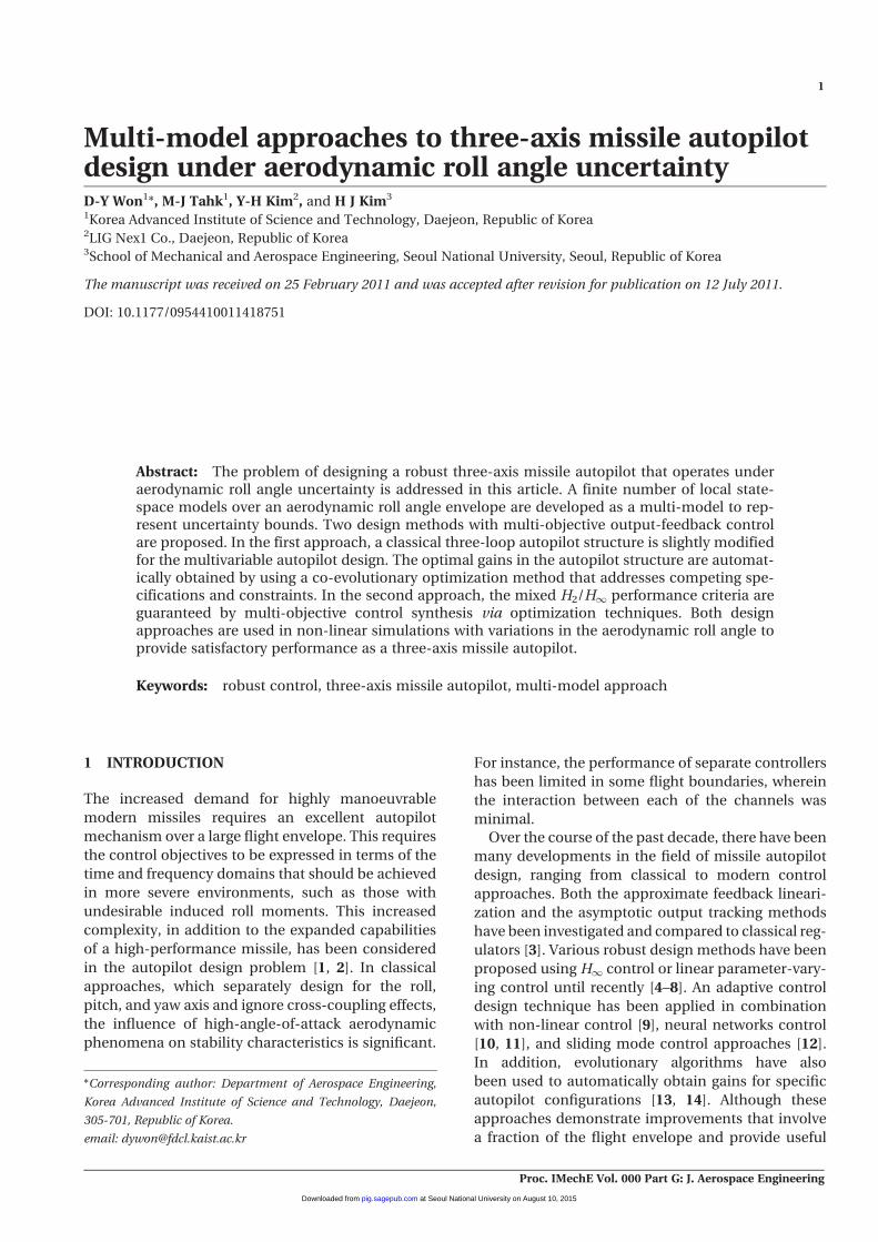
tions for �, �, �0, and �0 are depicted in Fig. 1 with the
aeroballistic wind coordinate [23].
The missile under consideration has a large flight
envelope that includes high-angle-of-attack condi-
tions. The asymmetric airflow on the control sur-
faces generates induced roll moments that result
in control difficulties while operating in the
Fig. 1 Aeroballistic wind coordinate systems
Three-axis missile autopilot design 3
Proc. IMechE Vol. 000 Part G: J. Aerospace Engineering
at Seoul National University on August 10, 2015pig.sagepub.comDownloaded from
high-angle-of-attack regime. It is difficult to estimate
induced roll moments that are significantly affected
by M, �, and fin configurations. The effects of this
phenomenon can become more complicated as the
missile manoeuvres in a low Mach number and high-
angle-of-attack region. The angle of attack bound-
aries, which are mainly concerned in this article,
include vortex-free and symmetric vortex flow as
the angle of attack is increased from 0� to 25�. The
details of the cross-coupling effects that are caused
by simultaneous pitch and yaw manoeuvring can be
found in the authors’ previous work [16].
2.2 Multi-model approach
For a given missile control problem, the rapid estima-
tion of the aerodynamic roll angle �0 with sufficient
accuracy is not straightforward, whereas the total
incidence angle �0 is estimated by an observer.
Some difficulty arises because of the highly non-
linear aerodynamics in a high-angle-of-attack and a
lack of appropriate sensors for both the angle of
attack and the sideslip angle. Under this condition,
a gain scheduling technique, which is commonly
used in missile autopilot design to capture coupling
effects, is not applicable. Instead, robust control
approaches should be considered if the aerodynamic
roll angle cannot be chosen as a scheduling parame-
ter. As a result, the autopilot that was designed (with
respect to the nominal model that was linearized at a
specific aerodynamic roll angle) is expected to guar-
antee not only its robust stability but also the perfor-
mance for the different aerodynamic roll angle trim
conditions. To address this problem, a multi-model
that was linearized at multiple flight conditions was
constructed to address the aerodynamic roll angle
uncertainty. If can be identified one autopilot that
satisfies the stability and performance requirements
for the multi-model plant, that autopilot can be con-
sidered to provide robust stability and performance
under the aerodynamic roll angle uncertainty. This
consideration converts the autopilot design problem
into a multi-objective controller design problem.
Some uncertainty that was due to other modelling
errors can also be dealt with in the multi-model for-
mulation. Furthermore, the classical and mixed H2/
H1 output-feedback control design methods are
explored. In this article, a finite set of linearized
models are considered as a state-space form of the
multi-model plant
Am, Bm, Cm, Dmf g 2 Ai , Bi , Ci , Di : i 2 Sf g ð7Þ
where S9 {1,. . ., k}. Such a multi-model may result
from the frequency bounds on the possible plant
perturbations. As a consequence, it is desirable to
find an output-feedback controller that satisfies the
given performance requirements via the classical
and mixed H2/H1} control approaches. To accom-
plish this, the controller design procedure that is
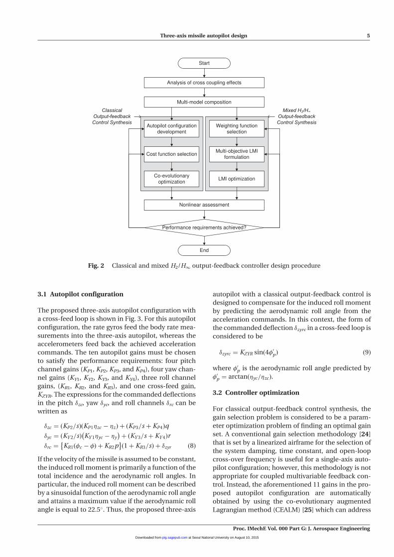
outlined in Fig. 2 is used and this design is discussed
in detail in the following sections. It is expected
that a missile autopilot that is designed in this
manner has a very high probability of success in an
actual plant due to its relatively small computational
load.
2.3 Autopilot performance requirements
The goal of the autopilot design is to steers the missile
to track the acceleration guidance commands that are
generated by an outer loop and stabilize the missile
airframe at a given bank angle. In particular, the sta-
bilization of the bank angle is a critical requirement
for controlling a highly manoeuvrable missile. The
performance goals for the three-axis autopilot
design are as follows.
1. Maintain robust stability over the operating range
that is specified by �0 such that 0�<�0< 180�. This
robustness refers to the uncertainty in the induced
roll moment, which has a significant effect in high-
angle-of-attack regime.
2. Track the step acceleration commands with a time
constant of less than 0.50 s, maximum overshoot
and undershoot of less than 20 per cent, and
steady-state error of less than 5 per cent.
3 CLASSICAL OUTPUT-FEEDBACK CONTROLSYNTHESIS
In this section, a multi-model approach is pre-
sented to classical output-feedback control synthe-
sis using the same three steps that are outlined in
Fig. 2. The first step involves developing an appro-
priate autopilot configuration to compensate for
the effects of cross-coupling. Previously, missile
autopilot design has been achieved using the roll,
pitch, and yaw channels. However, highly coupled
dynamics in agile maneuvers degrade the control
performance of a decoupled autopilot structure.
In this article, a three-loop autopilot with a cross-
feed loop is proposed to address cross-coupling
effects in the entire flight envelope. The second
and third steps are related to obtaining a combina-
tion of gains that satisfy the control performance
requirements using co-evolutionary optimization.
This controller optimization method provides a
useful way to address the multivariable feedback
controller design problems.
4 D-Y Won, M-J Tahk, Y-H Kim, and H J Kim
Proc. IMechE Vol. 000 Part G: J. Aerospace Engineering
at Seoul National University on August 10, 2015pig.sagepub.comDownloaded from
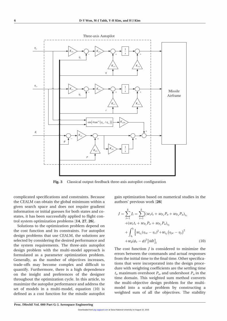
3.1 Autopilot configuration
The proposed three-axis autopilot configuration with
a cross-feed loop is shown in Fig. 3. For this autopilot
configuration, the rate gyros feed the body rate mea-
surements into the three-axis autopilot, whereas the
accelerometers feed back the achieved acceleration
commands. The ten autopilot gains must be chosen
to satisfy the performance requirements: four pitch
channel gains (KP1, KP2, KP3, and KP4), four yaw chan-
nel gains (KY1, KY2, KY3, and KY4), three roll channel
gains, (KR1, KR2, and KR3), and one cross-feed gain,
KZYR. The expressions for the commanded deflections
in the pitch �zc, yaw �yc, and roll channels �rc can be
written as
�zc ¼ KP2=sð Þ KP1�zc � �zð Þ þ KP3=s þ KP4ð Þq
�yc ¼ KY 2=sð Þ KY 1�yc � �y
� �þ KY 3=s þ KY 4ð Þr
�rc ¼ KR1 �c � �ð Þ þ KR2p� �
1þ KR3=sð Þ þ �zyr ð8Þ
If the velocity of the missile is assumed to be constant,
the induced roll moment is primarily a function of the
total incidence and the aerodynamic roll angles. In
particular, the induced roll moment can be described
by a sinusoidal function of the aerodynamic roll angle
and attains a maximum value if the aerodynamic roll
angle is equal to 22.5�. Thus, the proposed three-axis
autopilot with a classical output-feedback control is
designed to compensate for the induced roll moment
by predicting the aerodynamic roll angle from the
acceleration commands. In this context, the form of
the commanded deflection �zyrc in a cross-feed loop is
considered to be
�zyrc ¼ KZYR sinð4�0pÞ ð9Þ
where �0p is the aerodynamic roll angle predicted by
�0p ¼ arctanð�yc=�zc Þ.
3.2 Controller optimization
For classical output-feedback control synthesis, the
gain selection problem is considered to be a param-
eter optimization problem of finding an optimal gain
set. A conventional gain selection methodology [24]
that is set by a linearized airframe for the selection of
the system damping, time constant, and open-loop
cross-over frequency is useful for a single-axis auto-
pilot configuration; however, this methodology is not
appropriate for coupled multivariable feedback con-
trol. Instead, the aforementioned 11 gains in the pro-
posed autopilot configuration are automatically
obtained by using the co-evolutionary augmented
Lagrangian method (CEALM) [25] which can address
Fig. 2 Classical and mixed H2/H1 output-feedback controller design procedure
Three-axis missile autopilot design 5
Proc. IMechE Vol. 000 Part G: J. Aerospace Engineering
at Seoul National University on August 10, 2015pig.sagepub.comDownloaded from
complicated specifications and constraints. Because
the CEALM can obtain the global minimum within a
given search space and does not require gradient
information or initial guesses for both states and co-
states, it has been successfully applied to flight con-
trol system optimization problems [14, 27, 26].
Solutions to the optimization problem depend on
the cost function and its constraints. For autopilot
design problems that use CEALM, the solutions are
selected by considering the desired performance and
the system requirements. The three-axis autopilot
design problem with the multi-model approach is
formulated as a parameter optimization problem.
Generally, as the number of objectives increases,
trade-offs may become complex and difficult to
quantify. Furthermore, there is a high dependence
on the insight and preferences of the designer
throughout the optimization cycle. In this article, to
maximize the autopilot performance and address the
set of models in a multi-model, equation (10) is
defined as a cost function for the missile autopilot
gain optimization based on numerical studies in the
authors’ previous work [26]
J ¼Xk
i¼1
Ji ¼Xk
i¼1
ðwsts þwPoPo þwPu
Pu�z
�
þðwsts þwPoPo þwPu
Pu�y
þ
Z tf
t0
w�z�zc � �zð Þ
2þw�y
�yc � �y
� �2n
þw� �c � �ð Þ2�
tdt�
ið10Þ
The cost function J is considered to minimize the
errors between the commands and actual responses
from the initial time to the final time. Other specifica-
tions that were incorporated into the design proce-
dure with weighting coefficients are the settling time
ts, maximum overshoot Po, and undershoot Pu in the
time domain. This weighted sum method converts
the multi-objective design problem for the multi-
model into a scalar problem by constructing a
weighted sum of all the objectives. The stability
Fig. 3 Classical output-feedback three-axis autopilot configuration
6 D-Y Won, M-J Tahk, Y-H Kim, and H J Kim
Proc. IMechE Vol. 000 Part G: J. Aerospace Engineering
at Seoul National University on August 10, 2015pig.sagepub.comDownloaded from
margins, which are given in terms of the gain and
phase margins in the frequency domain, are consid-
ered as the constraints with the maximum overshoot
and undershoot as follows
GM 4GMd
PM 4PMd
Po 5Pod
Pu 5Pud ð11Þ
4 MIXED H2/H1 OUTPUT-FEEDBACKCONTROL SYNTHESIS
This section gives an overview of the multi-model
approach to the mixed H2/H1 output-feedback con-
trol synthesis, as outlined in Fig. 2. For this design
approach, the cost function selection problem in
classical output-feedback control synthesis becomes
an LMI formulation problem and includes the H1and H2 performances, which are subject to robust-
ness for the given multi-model description. The H1performance is convenient for enforcing the robust-
ness of the model uncertainty and expressing fre-
quency-domain specifications. The H2 performance
is useful for addressing the output (or error) power of
the generalized system due to a unit intensity white
noise input. For the output-feedback case, the dimen-
sions of the resulting controller that solve the H2/H1problem do not exceed the dimensions of the gener-
alized plant.
To implement the proposed mixed H2/H1 output-
feedback control, one of the generalized plants for the
multi-model composition of the following state-
space form is represented
_xzy
24
35 ¼
A B1 B2
C1 D11 D12
C2 D21 D22
24
35 x
!u
24
35 ð12Þ
where A2Rn�n, D122Rp1�m2, and D212Rp2�m1, while
x, u, z, y, and w are the state, control input, controlled
output, measurement output, and exogenous input,
respectively. Then, the multi-objective control prob-
lem is to find an LTI control law u¼K(s)y that mini-
mizes an upper bound for the H2 gain subject to the
H1 gain constraint. In a mixed H2/H1 control prob-
lem, the following assumptions [20] are made for the
each of generalized plants.
1. (A, B2, C2) is stabilizable and detectable.
2. D12 and D21 have full rank.
3.A � j!I B2
C1 D12
� has full column rank for all !.
4.A � j!I B1
C2 D21
� has full row rank for all !.
5. D11¼ 0 and D22¼ 0.
Assumption (A1) is required for the existence of a
stabilizing controller K, and assumption (A2) is suffi-
cient to guarantee the controller is proper and realiz-
able. Assumptions (A3) and (A4) ensure that the
controller does not attempt to cancel poles or zeros
on the imaginary axis which would result in closed-
loop instability. Assumption (A5) is typically made in
H2 control.
4.1 Multi-objective LMI formulation
LMI formulations for the multi-model approach to
the mixed H2/H1 output-feedback control are intro-
duced. For brevity, multi-objective LMI formulations
for a single-model case are described. After than
extension of LMI formulations to a multi-model
case is established subsequently. If all design objec-
tives are formulated in terms of a common Lyapunov
function, controller design is emerged to solve a
system of LMIs. The resulting LMI formulations are
induced from the multi-objective control synthesis
[21, 22].
The LTI controller K(s) can be represented in state-
space form by
_xK tð Þ ¼ AK xK tð Þ þ BK y tð Þ
u tð Þ ¼ CK xK tð Þ þDK y tð Þ ð13Þ
For LMI approach to multi-objective synthesis, non-
linear terms added in the output feedback case
should be eliminated by some appropriate change
of controller variables. This change of controller var-
iables is implicitly defined in terms of the Lyapunov
matrix P.
P ¼Y N
N T V
� , P�1 ¼
X MM T U
� ð14Þ
where X2Rn�n and Y2Rn�n are symmetric. The new
controller variables can be written by
AK :¼ NAK M T þNBK C2X þ YBCK M T
þY A þ B2DK C2ð ÞX ,
BK :¼ NBK þ YB2DK ,
CK :¼ CK M T þDK C2X ,
DK :¼ DK : ð15Þ
8>>>>><>>>>>:
Then, the mixed H2/H1 synthesis would be finding
X , Y , AK , BK , CK , and DK such that equations (16) to
(20) are hold, while minimizing � and
�11 �T21 �T
31 �T41
�21 �22 �T32 �T
42
�31 �32 �33 �T43
�41 �42 �43 �44
2664
37755 0 ð16Þ
Three-axis missile autopilot design 7
Proc. IMechE Vol. 000 Part G: J. Aerospace Engineering
at Seoul National University on August 10, 2015pig.sagepub.comDownloaded from
�11 �T21 �T
31
�21 �22 �T32
�31 �32 �33
24
355 0 ð17Þ
X I �
I Y �
C1X þD12CK C1 þD12DK C2 Q
24
354 0 ð18Þ
Tr Qð Þ5 ð19Þ
ðD11 þD12DK D21Þ ¼ 0 ð20Þ
with the shorthand notation
�11 :¼ AX þ XAT þ BCK þ ðBCK ÞT
�21 :¼ AK þ ðA þ B2DK C2ÞT
�22 :¼ AT Y þ YA þ BK C2 þ ðBK C2ÞT
�31 :¼ ðB1 þ B2DK D21ÞT
�32 :¼ ðYB1 þ BK D21ÞT
�33 :¼ ��I
�41 :¼ C1X þD12CK
�42 :¼ C1 þD12DK C2
�43 :¼ D11 þD12DK D21
�44 :¼ ��I ð21Þ
�11 :¼ AX þ XAT þ B2CK þ ðB2CK ÞT
�21 :¼ AK þ ðA þ B2DK C2ÞT
�22 :¼ AT Y þ YA þ BK C2 þ ðBK C2ÞT
�31 :¼ ðB1 þ B2DK D21ÞT
�32 :¼ ðYB1 þ BK D21ÞT
�33 :¼ �I ð22Þ
The previous formulations are directly extended to
uncertain systems described by the multi-model
approach. Note that LMI conditions for H2 and H1performances over the set of linear models are
obtained similarly by writing equations (16) to (20)
for each of the linear model components.
4.2 Controller computation
The multi-objective output-feedback synthesis is an
LMI problem of the form
Minimize � þ over X , Y , AK , BK , CK , DK , �,
satisfying equations ð16Þ to ð20Þ: ð23Þ
After solving the synthesis LMI formulations, the con-
troller computation proceeds as follows:
1. Find non-singular matrix M, N to satisfy
MNT¼ I�XY via singular value decomposition.
2. Solve equation (15) for the controller K(s)
DK :¼ DK ,
CK :¼ CK �DK C2X �
M�T ,
BK :¼ N�1 BK � YB2DK
�,
AK :¼ N�1 AK �NBK C2X � YB2CK M T
�Y A þ B2DK C2ð ÞX ÞM�T
8>>>>>>><>>>>>>>:
ð24Þ
This LMI optimization problem can be efficiently
solved using the LMI Control Toolbox [28]. The
given LMI problem is solvable if and only if the LMI
conditions given by equations (16) to (20) are feasible.
Because H1 and H2 constraints are removed in the
LMI problem, the LMI conditions become necessary
and sufficient. Related proofs can be found in refer-
ence [21]. The solution of the LMI problem gives an
upper estimate of the suboptimal H1 and H2 perfor-
mance. For the output-feedback control synthesis, a
set of controllers which depend on the system
dynamics are obtained instead of a single controller,
since equation (24) involves the terms of the system
matrix (A, B2, C2). The dependency caused by the
nature of output-feedback control cannot be
removed by a change of variables directly. For this
reason, controller switching between computed con-
trollers is employed based on the predicted aerody-
namic roll angle �0p from the acceleration commands.
The points of the controller switching are determined
by the selected operating points for the multi-model
construction. This scheme can be considered as gain-
scheduling control in that controller switching
depends on commands, not state variables. Note
that the predicted aerodynamic roll angle is also
used in the cross-feed loop of the classical output-
feedback controller.
4.3 Interconnected system model
The mixed H2/H1 control approach for characteriz-
ing the closed-loop performance objectives is to mea-
sure the norms of the closed-loop transfer function
matrices. Because a natural performance objective is
to provide a closed-loop gain from exogenous influ-
ences, ! (reference commands r, sensor noise n, and
external force disturbances d), to the regulated vari-
ables (tracking errors e and control input u), the per-
formance specifications for the closed-loop system in
terms of multi-objective control can be defined as
follows.
1. Guarantee an upper bound on the � of the operator
mapping z1 to !.
2. Minimize an upper bound on the variance of z2 due
to the disturbance !.
8 D-Y Won, M-J Tahk, Y-H Kim, and H J Kim
Proc. IMechE Vol. 000 Part G: J. Aerospace Engineering
at Seoul National University on August 10, 2015pig.sagepub.comDownloaded from
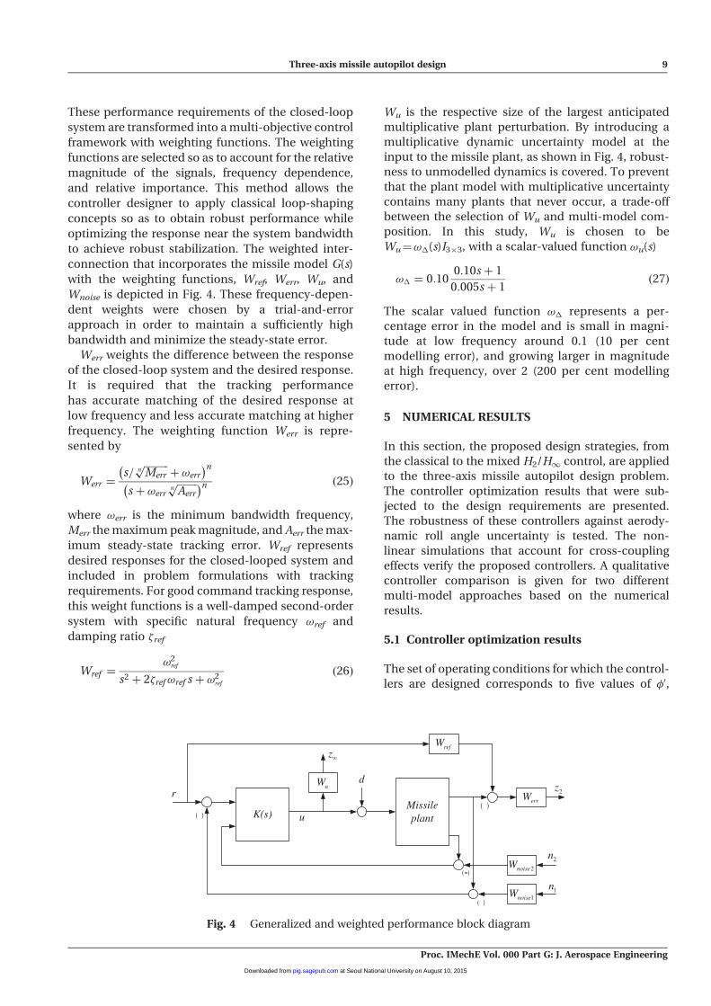
These performance requirements of the closed-loop
system are transformed into a multi-objective control
framework with weighting functions. The weighting
functions are selected so as to account for the relative
magnitude of the signals, frequency dependence,
and relative importance. This method allows the
controller designer to apply classical loop-shaping
concepts so as to obtain robust performance while
optimizing the response near the system bandwidth
to achieve robust stabilization. The weighted inter-
connection that incorporates the missile model G(s)
with the weighting functions, Wref, Werr, Wu, and
Wnoise is depicted in Fig. 4. These frequency-depen-
dent weights were chosen by a trial-and-error
approach in order to maintain a sufficiently high
bandwidth and minimize the steady-state error.
Werr weights the difference between the response
of the closed-loop system and the desired response.
It is required that the tracking performance
has accurate matching of the desired response at
low frequency and less accurate matching at higher
frequency. The weighting function Werr is repre-
sented by
Werr ¼s=
ffiffiffiffiffiffiffiffiffiffiMerr
np
þ !err
� �n
s þ !err
ffiffiffiffiffiffiffiffiAerr
np� �n ð25Þ
where !err is the minimum bandwidth frequency,
Merr the maximum peak magnitude, and Aerr the max-
imum steady-state tracking error. Wref represents
desired responses for the closed-looped system and
included in problem formulations with tracking
requirements. For good command tracking response,
this weight functions is a well-damped second-order
system with specific natural frequency !ref and
damping ratio �ref
Wref ¼!2
ref
s2 þ 2�ref !ref s þ !2ref
ð26Þ
Wu is the respective size of the largest anticipated
multiplicative plant perturbation. By introducing a
multiplicative dynamic uncertainty model at the
input to the missile plant, as shown in Fig. 4, robust-
ness to unmodelled dynamics is covered. To prevent
that the plant model with multiplicative uncertainty
contains many plants that never occur, a trade-off
between the selection of Wu and multi-model com-
position. In this study, Wu is chosen to be
Wu¼!�(s)I3�3, with a scalar-valued function !u(s)
!� ¼ 0:100:10s þ 1
0:005s þ 1ð27Þ
The scalar valued function !� represents a per-
centage error in the model and is small in magni-
tude at low frequency around 0.1 (10 per cent
modelling error), and growing larger in magnitude
at high frequency, over 2 (200 per cent modelling
error).
5 NUMERICAL RESULTS
In this section, the proposed design strategies, from
the classical to the mixed H2/H1 control, are applied
to the three-axis missile autopilot design problem.
The controller optimization results that were sub-
jected to the design requirements are presented.
The robustness of these controllers against aerody-
namic roll angle uncertainty is tested. The non-
linear simulations that account for cross-coupling
effects verify the proposed controllers. A qualitative
controller comparison is given for two different
multi-model approaches based on the numerical
results.
5.1 Controller optimization results
The set of operating conditions for which the control-
lers are designed corresponds to five values of �0,
Fig. 4 Generalized and weighted performance block diagram
Three-axis missile autopilot design 9
Proc. IMechE Vol. 000 Part G: J. Aerospace Engineering
at Seoul National University on August 10, 2015pig.sagepub.comDownloaded from
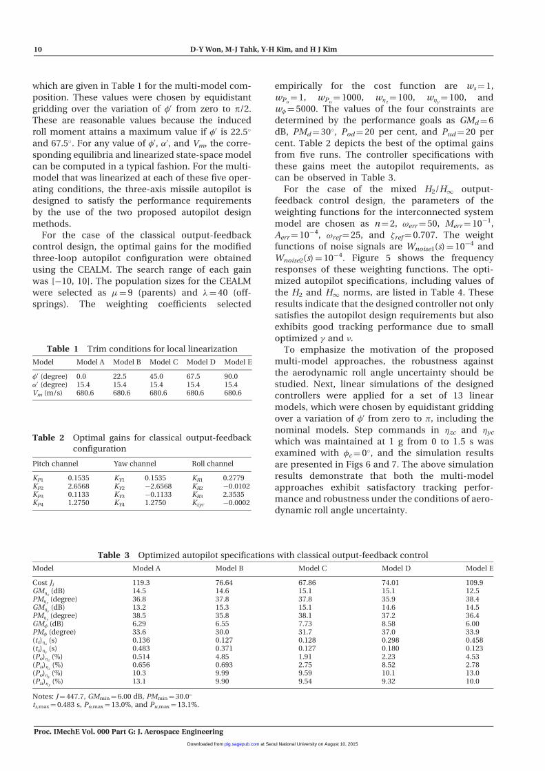
which are given in Table 1 for the multi-model com-
position. These values were chosen by equidistant
gridding over the variation of �0 from zero to p/2.
These are reasonable values because the induced
roll moment attains a maximum value if �0 is 22.5�
and 67.5�. For any value of �0, �0, and Vm, the corre-
sponding equilibria and linearized state-space model
can be computed in a typical fashion. For the multi-
model that was linearized at each of these five oper-
ating conditions, the three-axis missile autopilot is
designed to satisfy the performance requirements
by the use of the two proposed autopilot design
methods.
For the case of the classical output-feedback
control design, the optimal gains for the modified
three-loop autopilot configuration were obtained
using the CEALM. The search range of each gain
was [�10, 10]. The population sizes for the CEALM
were selected as ¼ 9 (parents) and �¼ 40 (off-
springs). The weighting coefficients selected
empirically for the cost function are ws¼ 1,
wPo¼ 1, wPu
¼ 1000, w�z¼ 100, w�y
¼ 100, and
w�¼ 5000. The values of the four constraints are
determined by the performance goals as GMd¼ 6
dB, PMd¼ 30�, Pod¼ 20 per cent, and Pud¼ 20 per
cent. Table 2 depicts the best of the optimal gains
from five runs. The controller specifications with
these gains meet the autopilot requirements, as
can be observed in Table 3.
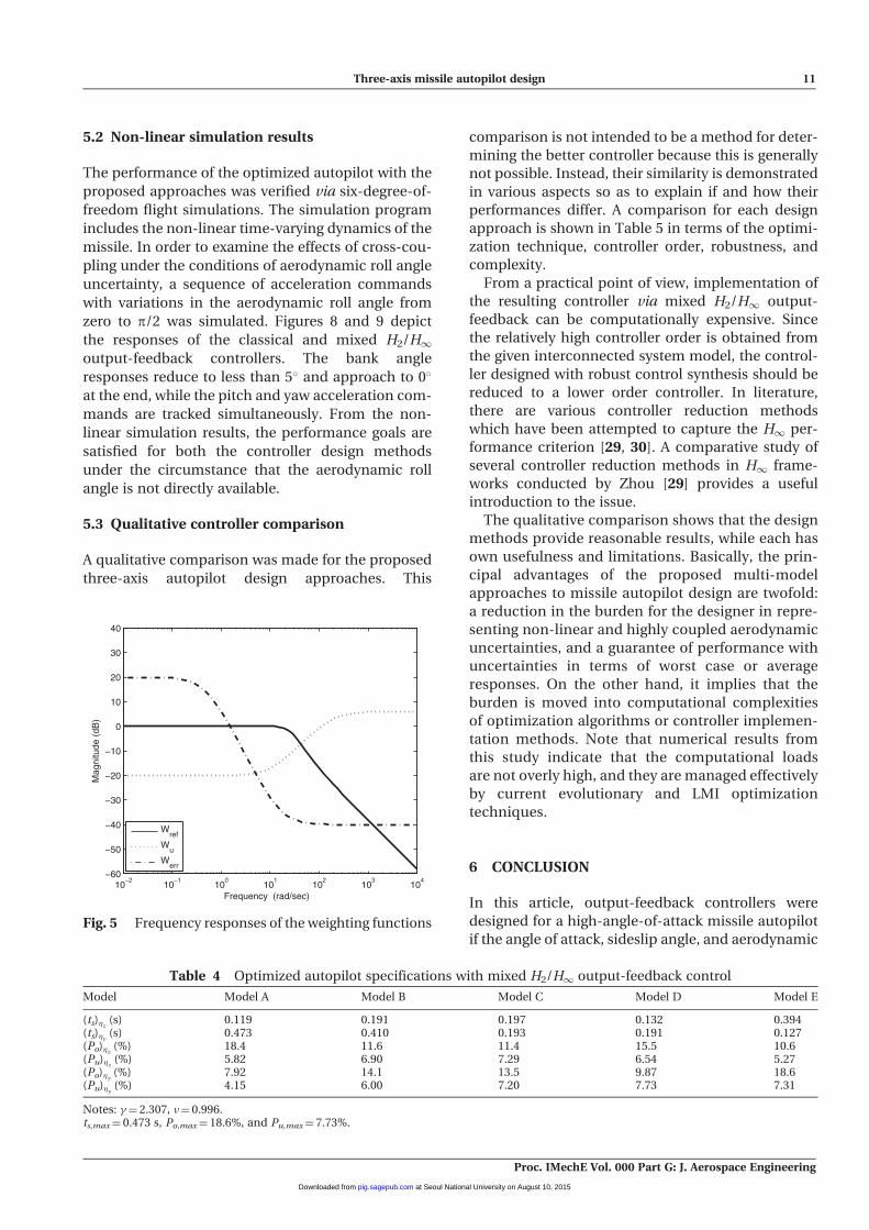
For the case of the mixed H2/H1 output-
feedback control design, the parameters of the
weighting functions for the interconnected system
model are chosen as n¼ 2, !err¼ 50, Merr¼ 10�1,
Aerr¼ 10�4, !ref¼ 25, and �ref¼ 0.707. The weight
functions of noise signals are Wnoise1(s)¼ 10�4 and
Wnoise2(s)¼ 10�4. Figure 5 shows the frequency
responses of these weighting functions. The opti-
mized autopilot specifications, including values of
the H2 and H1 norms, are listed in Table 4. These
results indicate that the designed controller not only
satisfies the autopilot design requirements but also
exhibits good tracking performance due to small
optimized � and .
To emphasize the motivation of the proposed
multi-model approaches, the robustness against
the aerodynamic roll angle uncertainty should be
studied. Next, linear simulations of the designed
controllers were applied for a set of 13 linear
models, which were chosen by equidistant gridding
over a variation of �0 from zero to �, including the
nominal models. Step commands in �zc and �yc
which was maintained at 1 g from 0 to 1.5 s was
examined with �c¼ 0�, and the simulation results
are presented in Figs 6 and 7. The above simulation
results demonstrate that both the multi-model
approaches exhibit satisfactory tracking perfor-
mance and robustness under the conditions of aero-
dynamic roll angle uncertainty.
Table 3 Optimized autopilot specifications with classical output-feedback control
Model Model A Model B Model C Model D Model E
Cost Ji 119.3 76.64 67.86 74.01 109.9GM�z
(dB) 14.5 14.6 15.1 15.1 12.5PM�z
(degree) 36.8 37.8 37.8 35.9 38.4GM�y
(dB) 13.2 15.3 15.1 14.6 14.5PM�y
(degree) 38.5 35.8 38.1 37.2 36.4GM� (dB) 6.29 6.55 7.73 8.58 6.00PM� (degree) 33.6 30.0 31.7 37.0 33.9(ts)�z
(s) 0.136 0.127 0.128 0.298 0.458(ts)�y
(s) 0.483 0.371 0.127 0.180 0.123(Po)�z
(%) 0.514 4.85 1.91 2.23 4.53(Pu)�z
(%) 0.656 0.693 2.75 8.52 2.78(Po)�y
(%) 10.3 9.99 9.59 10.1 13.0(Pu)�y
(%) 13.1 9.90 9.54 9.32 10.0
Notes: J¼ 447.7, GMmin¼ 6.00 dB, PMmin¼ 30.0�
ts,max¼ 0.483 s, Po,max¼ 13.0%, and Pu,max¼ 13.1%.
Table 2 Optimal gains for classical output-feedback
configuration
Pitch channel Yaw channel Roll channel
KP1 0.1535 KY1 0.1535 KR1 0.2779KP2 2.6568 KY2 �2.6568 KR2 �0.0102KP3 0.1133 KY3 �0.1133 KR3 2.3535KP4 1.2750 KY4 1.2750 Kzyr �0.0002
Table 1 Trim conditions for local linearization
Model Model A Model B Model C Model D Model E
�0 (degree) 0.0 22.5 45.0 67.5 90.0�0 (degree) 15.4 15.4 15.4 15.4 15.4Vm (m/s) 680.6 680.6 680.6 680.6 680.6
10 D-Y Won, M-J Tahk, Y-H Kim, and H J Kim
Proc. IMechE Vol. 000 Part G: J. Aerospace Engineering
at Seoul National University on August 10, 2015pig.sagepub.comDownloaded from
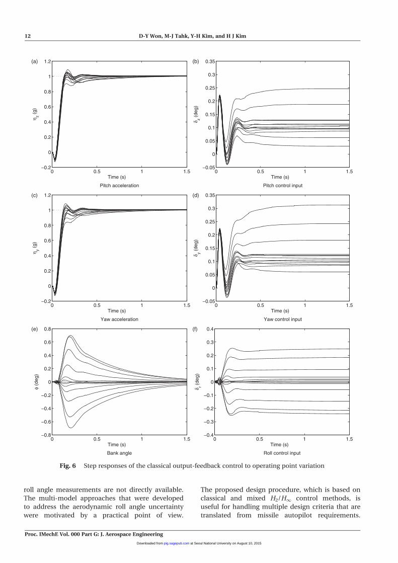
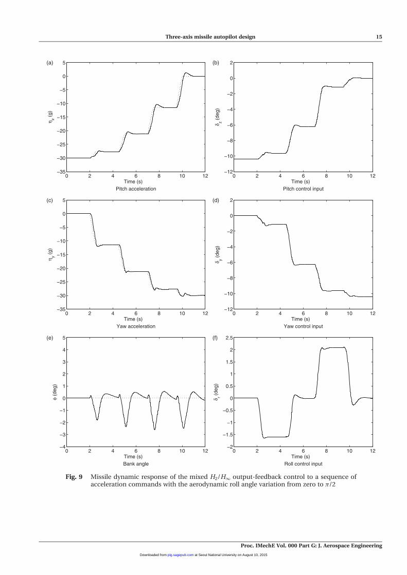
5.2 Non-linear simulation results
The performance of the optimized autopilot with the
proposed approaches was verified via six-degree-of-
freedom flight simulations. The simulation program
includes the non-linear time-varying dynamics of the
missile. In order to examine the effects of cross-cou-
pling under the conditions of aerodynamic roll angle
uncertainty, a sequence of acceleration commands
with variations in the aerodynamic roll angle from
zero to p/2 was simulated. Figures 8 and 9 depict
the responses of the classical and mixed H2/H1output-feedback controllers. The bank angle
responses reduce to less than 5� and approach to 0�
at the end, while the pitch and yaw acceleration com-
mands are tracked simultaneously. From the non-
linear simulation results, the performance goals are
satisfied for both the controller design methods
under the circumstance that the aerodynamic roll
angle is not directly available.
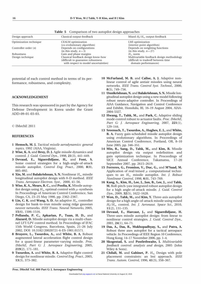
5.3 Qualitative controller comparison
A qualitative comparison was made for the proposed
three-axis autopilot design approaches. This
comparison is not intended to be a method for deter-
mining the better controller because this is generally
not possible. Instead, their similarity is demonstrated
in various aspects so as to explain if and how their
performances differ. A comparison for each design
approach is shown in Table 5 in terms of the optimi-
zation technique, controller order, robustness, and
complexity.
From a practical point of view, implementation of
the resulting controller via mixed H2/H1 output-
feedback can be computationally expensive. Since
the relatively high controller order is obtained from
the given interconnected system model, the control-
ler designed with robust control synthesis should be
reduced to a lower order controller. In literature,
there are various controller reduction methods
which have been attempted to capture the H1 per-
formance criterion [29, 30]. A comparative study of
several controller reduction methods in H1 frame-
works conducted by Zhou [29] provides a useful
introduction to the issue.
The qualitative comparison shows that the design
methods provide reasonable results, while each has
own usefulness and limitations. Basically, the prin-
cipal advantages of the proposed multi-model
approaches to missile autopilot design are twofold:
a reduction in the burden for the designer in repre-
senting non-linear and highly coupled aerodynamic
uncertainties, and a guarantee of performance with
uncertainties in terms of worst case or average
responses. On the other hand, it implies that the
burden is moved into computational complexities
of optimization algorithms or controller implemen-
tation methods. Note that numerical results from
this study indicate that the computational loads
are not overly high, and they are managed effectively
by current evolutionary and LMI optimization
techniques.
6 CONCLUSION
In this article, output-feedback controllers were
designed for a high-angle-of-attack missile autopilot
if the angle of attack, sideslip angle, and aerodynamic
Table 4 Optimized autopilot specifications with mixed H2/H1 output-feedback control
Model Model A Model B Model C Model D Model E
(ts)�z(s) 0.119 0.191 0.197 0.132 0.394
(ts)�y(s) 0.473 0.410 0.193 0.191 0.127
(Po)�z(%) 18.4 11.6 11.4 15.5 10.6
(Pu)�z(%) 5.82 6.90 7.29 6.54 5.27
(Po)�y(%) 7.92 14.1 13.5 9.87 18.6
(Pu)�y(%) 4.15 6.00 7.20 7.73 7.31
Notes: �¼ 2.307, ¼ 0.996.ts,max¼ 0.473 s, Po,max¼ 18.6%, and Pu,max¼ 7.73%.
Frequency (rad/sec)10
−210
−110
010
110
210
310
4−60
−50
−40
−30
−20
−10
0
10
20
30
40
Mag
nitu
de (
dB)
Wref
Wu
Werr
Fig. 5 Frequency responses of the weighting functions
Three-axis missile autopilot design 11
Proc. IMechE Vol. 000 Part G: J. Aerospace Engineering
at Seoul National University on August 10, 2015pig.sagepub.comDownloaded from
roll angle measurements are not directly available.
The multi-model approaches that were developed
to address the aerodynamic roll angle uncertainty
were motivated by a practical point of view.
The proposed design procedure, which is based on
classical and mixed H2/H1 control methods, is
useful for handling multiple design criteria that are
translated from missile autopilot requirements.
0 0.5 1 1.5−0.2
0
0.2
0.4
0.6
0.8
1
1.2(a) (b)
(c) (d)
(e) (f)
Time (s)
η z (g)
0 0.5 1 1.5−0.05
0
0.05
0.1
0.15
0.2
0.25
0.3
0.35
Time (s)
δ z (de
g)
0 0.5 1 1.5−0.2
0
0.2
0.4
0.6
0.8
1
1.2
Time (s)
η y (g)
0 0.5 1 1.5−0.05
0
0.05
0.1
0.15
0.2
0.25
0.3
0.35
Time (s)
δ y (de
g)
0 0.5 1 1.5−0.8
−0.6
−0.4
−0.2
0
0.2
0.4
0.6
0.8
Time (s)
φ (d
eg)
0 0.5 1 1.5−0.4
−0.3
−0.2
−0.1
0
0.1
0.2
0.3
0.4
Time (s)
Pitch acceleration Pitch control input
Yaw acceleration Yaw control input
Bank angle Roll control input
δ r (de
g)
Fig. 6 Step responses of the classical output-feedback control to operating point variation
12 D-Y Won, M-J Tahk, Y-H Kim, and H J Kim
Proc. IMechE Vol. 000 Part G: J. Aerospace Engineering
at Seoul National University on August 10, 2015pig.sagepub.comDownloaded from
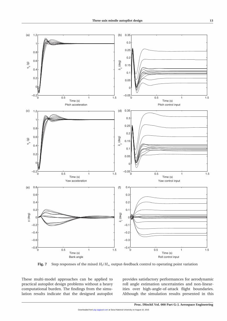
These multi-model approaches can be applied to
practical autopilot design problems without a heavy
computational burden. The findings from the simu-
lation results indicate that the designed autopilot
provides satisfactory performances for aerodynamic
roll angle estimation uncertainties and non-linear-
ities over high-angle-of-attack flight boundaries.
Although the simulation results presented in this
0 0.5 1 1.5−0.2
0
0.2
0.4
0.6
0.8
1
1.2(a) (b)
(c) (d)
(e) (f)
Time (s)
η z (g)
0 0.5 1 1.5−0.05
0
0.05
0.1
0.15
0.2
0.25
0.3
0.35
Time (s)
δ z (de
g)
0 0.5 1 1.5−0.2
0
0.2
0.4
0.6
0.8
1
1.2
Time (s)
η y (g)
0 0.5 1 1.5−0.05
0
0.05
0.1
0.15
0.2
0.25
0.3
0.35
Time (s)
δ y (de
g)
0 0.5 1 1.5−0.8
−0.6
−0.4
−0.2
0
0.2
0.4
0.6
0.8
Time (s)
φ (d
eg)
0 0.5 1 1.5−0.4
−0.3
−0.2
−0.1
0
0.1
0.2
0.3
0.4
Time (s)
Pitch acceleration Pitch control input
Yaw acceleration Yaw control input
Bank angle Roll control input
δ r (de
g)
Fig. 7 Step responses of the mixed H2/H1 output-feedback control to operating point variation
Three-axis missile autopilot design 13
Proc. IMechE Vol. 000 Part G: J. Aerospace Engineering
at Seoul National University on August 10, 2015pig.sagepub.comDownloaded from

article only illustrate the formulations for the com-
pensation of cross-coupling effects under aerody-
namic roll angle uncertainty, further testing is
required to arrive at any conclusions regarding the
effectiveness of multi-model approaches to missile
autopilot design problems. A qualitative comparison
between the proposed control methods provides
guidelines to controller designers for evaluating the
0 2 4 6 8 10 12−35
−30
−25
−20
−15
−10
−5
0
5(a) (b)
(c) (d)
(e) (f)
η z (g)
Time (s)0 2 4 6 8 10 12
−12
−10
−8
−6
−4
−2
0
2
Time (s)
δ z (de
g)
0 2 4 6 8 10 12−35
−30
−25
−20
−15
−10
−5
0
5
η y (g)
Time (s)0 2 4 6 8 10 12
−12
−10
−8
−6
−4
−2
0
2
Time (s)
δ y (de
g)
0 2 4 6 8 10 12−4
−3
−2
−1
0
1
2
3
4
5
φ (d
eg)
Time (s)0 2 4 6 8 10 12
−2
−1.5
−1
−0.5
0
0.5
1
1.5
2
2.5
Time (s)
Pitch acceleration Pitch control input
Yaw acceleration Yaw control input
Bank angle Roll control input
δ r (de
g)
Fig. 8 Missile dynamic response of the classical output-feedback control to a sequence of accel-eration commands with the aerodynamic roll angle variation from zero to �/2
14 D-Y Won, M-J Tahk, Y-H Kim, and H J Kim
Proc. IMechE Vol. 000 Part G: J. Aerospace Engineering
at Seoul National University on August 10, 2015pig.sagepub.comDownloaded from
0 2 4 6 8 10 12−35
−30
−25
−20
−15
−10
−5
0
5(a) (b)
(c) (d)
(e) (f)
η z (g)
Time (s)0 2 4 6 8 10 12
−12
−10
−8
−6
−4
−2
0
2
Time (s)
δ z (de
g)
0 2 4 6 8 10 12−35
−30
−25
−20
−15
−10
−5
0
5
η y (g)
Time (s)0 2 4 6 8 10 12
−12
−10
−8
−6
−4
−2
0
2
Time (s)
δ y (de
g)
0 2 4 6 8 10 12−4
−3
−2
−1
0
1
2
3
4
5
φ (d
eg)
Time (s)0 2 4 6 8 10 12
−2
−1.5
−1
−0.5
0
0.5
1
1.5
2
2.5
Time (s)
Pitch acceleration Pitch control input
Yaw acceleration Yaw control input
Bank angle Roll control input
δ r (de
g)
Fig. 9 Missile dynamic response of the mixed H2/H1 output-feedback control to a sequence ofacceleration commands with the aerodynamic roll angle variation from zero to �/2
Three-axis missile autopilot design 15
Proc. IMechE Vol. 000 Part G: J. Aerospace Engineering
at Seoul National University on August 10, 2015pig.sagepub.comDownloaded from
potential of each control method in terms of its per-
formance, robustness, and complexity.
ACKNOWLEDGEMENT
This research was sponsored in part by the Agency for
Defense Development in Korea under the Grant
ADD-09-01-03-03.
� IMechE 2011
REFERENCES
1 Hemsch, M. J. Tactical missile aerodynamics: generaltopics, 1992 (AIAA, Virginia).
2 Wise, K. A. and Broy, D. J. Agile missile dynamics andcontrol. J. Guid. Control Dyn., 1998, 21(3), 441–449.
3 Devaud, E., Siguerdidjane, H., and Font, S.Some control strategies for a high-angle-of-attackmissile autopilot. Control Eng. Pract., 2000, 8(8),885–892.
4 Xin, M. and Balakrishnan, S. N. Nonlinear H1missilelongitudinal autopilot design with y–D method. IEEETrans. Aerospace Electron. Syst., 2000, 41–56.
5 Wise, K. A., Mears, B. C., and Poolia, K. Missile autop-ilot design using H1 optimal control with -synthesisIn Proceedings of American Control Conference, SanDiego, CA, 23–25 May 1990, pp. 2362–2367.
6 Lin, C. K. and Wang, S. D. An adaptive H1 controllerdesign for bank-to-trun missile using ridge gaussianneuver networks. IEEE Trans. Neural Networks, 2005,15(6), 1506–1516.
7 Pellanda, P. C., Apkarian, P., Tuan, H. D., andAlazard, D. Missile autopilot design via a multi-chan-nel LFT/LPV control method. In Proceedings of IFAC15th World Congress, Barcelona, Spain, 21–26 July2002, DOI: 10.3182/20020721-6-ES-1901.01571.
8 Bruyere, L., Tsourdos, A., and White, B. A. Robustaugmented lateral acceleration flight control designfor a quasi-linear parameter-varying missile. Proc.IMechE, Part G: J. Aerospace Engineering, 2005,219(2), 171–181.
9 Tsourdos, A. and White, B. A. Adaptive flight controldesign for nonlinear missile. Control Eng. Pract., 2005,13(3), 373–382.
10 McFarland, M. B. and Calise, A. J. Adaptive non-linear control of agile antiair missiles using neuralnetworks. IEEE Trans. Control Syst. Technol., 2000,8(5), 749–756.
11 Unnikrishnan, N. and Balakrishnan, S. N. Missile lon-gitudinal autopilot design using a new model followingrobust neuro-adaptive controller. In Proceedings ofAIAA Guidance, Navigation and Control Conferenceand Exhibit, Honolulu, RI, 16–19 August 2004, AIAA-2004-5327.
12 Hwang, T., Tahk, M., and Park, C. Adaptive slidingmode control robust to actuator faults. Proc. IMechE,Part G: J. Aerospace Engineering, 2007, 221(1),129–144.
13 Sreenuch, T., Tsourdos, A., Hughes, E. J., and White,B. A. Fuzzy gain-scheduled missile autopilot designusing evolutionary algorithms. In Proceedings ofAmerican Control Conference, Portland, OR, 8–10June 2005, pp. 346–351.
14 Min, B., Sang, D., Tahk, M., and Kim, B. Missileautopilot design via output redefinition andgain optimization technique. In Proceedings ofSICE Annual Conference, Takamatsu, 17–20September 2007, pp. 2615–2619.
15 Ferreres, G., Fromion, V., Duc, G., and M’Saad, M.Application of real/mixed computational techni-ques to an H1 missile autopilot. Int. J. RobustNonlinear Control, 1998, 6(8), 743–769.
16 Kang, S., Kim, H., Lee, J., Jun, B., Lee, J., and Tahk,M. Roll-pitch-yaw integrated robust autopilot designfor a high angle-of-attack missile. J. Guid. ControlDyn., 2009, 32(5), 1622–1628.
17 Won, D., Tahk, M., and Kim, Y. Three-axis autopilotdesign for a high angle-of-attack missile using mixedH2/H1 control. Int. J. Aeronaut. Space Sci., 2010,11(2), 131–135.
18 Devaud, E., Harcaut, J., and Siguerdidjane, H.Three-axes missile autopilot design: from linear tononlinear control strategies. J. Guid. Control Dyn.,2001, 24(1), 64–71.
19 Das, A., Das, R., Mukhopadhyay, S., and Patra, A.Robust three axes autopilot for a tactical aerospacevehicle. In Proceedings of IEEE Region 10 Conference,Hong Kong, 14–17 November 2006, pp. 1–4.
20 Skogestad, S. and Postlethwaite, I. Multivariablefeedback control: analysis and design, 2005 (JohnWiley & Sons).
21 Chilali, M. and Gahinet, P. H1 Design with poleplacement constraints: an lmi approach. IEEETrans. Autom. Control, 1996, 41(3), 358–367.
Table 5 Comparison of two autopilot design approaches
Design approach Classical output-feedback Mixed H2/H1 output-feedback
Optimization technique CEALM optimization LMI optimization(co-evolutionary algorithm) (interior-point algorithm)
Controller order (n) Depends on configurations Depends on weighting functions(in this study, n¼ 3) (in this study, n¼ 27)
Robustness Gain and phase margins H1 normDesign technique Classical feedback design know-how Multivariable feedback design methodology
(difficult to guarantee robustnesswith respect to model uncertainties)
(difficult to tradeoff between timedomain performances)
16 D-Y Won, M-J Tahk, Y-H Kim, and H J Kim
Proc. IMechE Vol. 000 Part G: J. Aerospace Engineering
at Seoul National University on August 10, 2015pig.sagepub.comDownloaded from
22 Scherer, C. and Gahinet, P. Multi-objective output-feedback control via LMI optimization. IEEE Trans.Autom. Control, 1997, 42(7), 896–911.
23 Zipfel, P. H. Modeling and simulation of aerospacevehicle dynamic, 2000 (AIAA, Virginia).
24 Zarchan, P. Tactical and strategic missile guidance.Progress in astronautics and aeronautics series, 2007(AIAA, Reston, VI).
25 Tahk, M. and Sun, B. Co-evolutionary augmentedlagrangian method for constrained optimization.IEEE Trans. Evolut. Comput., 2000, 4(2), 114–124.
26 Kim, Y., Won, D., Kim, T., Tahk, M., Jun, B., and Lee,J. Integrated roll-pitch-yaw autopilot design for mis-siles. KSAS Int. J., 2008, 9(1), 129–136.
27 Lee, H., Sun, B., Tahk, M., and Lee, H. Controldesign of spinning rockets based on co-evolutionaryoptimization. Control Eng. Pract., 2001, 9(2),149–157.
28 Gahinet, P., Nemirovskii, A., Laub, A. J., and Chilali,M. The LMI control toolbox. In Proceedings of 33rdIEEE Conference on Decision and Control, vol. 3,Lake Buena Vista, FL, 14–16 December 1994,pp. 2038–2041.
29 Zhou, K. A comparative study of H-infinitycontroller reduction methods. In ProceedingsAmerican Control Conference, Seattle, WA, 21–23June 1995, pp. 4015–4019.
30 Goddard, P. J. and Glover, K. Controller approxima-tion: approaches for preserving H1 performance.IEEE Trans. Autom. Control, 1998, 43(7), 858–871.
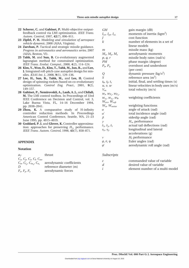
APPENDIX
Notation
aT thrust
Cx, Cy, Cz, Cl, Cm,
Cn, Clp, Cmq
, Cnraerodynamic coefficients
D reference diameter (m)
Fx, Fy, Fz aerodynamic forces
GM gain margin (dB)
Ixx, Iyy, Izz moments of inertia (kgm2)
J cost function
k number of elements in a set of
linear models
m missile mass (kg)
Mx, My, Mz aerodynamic moments
p, q, r missile body rates (rad/s)
PM phase margin (degree)
Po, Pu overshoot and undershoot
(per cent)
Q dynamic pressure (kg/s2)
S reference area (m2)
t0, tf, ts initial, final, and settling times (s)
u, v, w linear velocities in body axes (m/s)
Vm total velocity (m/s)
ws, wPo, wPu
,
w�z, w�y
, w� weighting coefficients
Werr, Wref,
Wu, Wnoise weighting functions
� angle of attack (rad)
�0 total incidence angle (rad)
� sideslip angle (rad)
� H1 performance
�z, �y, �r actual tail deflections (rad)
�z, �y longitudinal and lateral
accelerations (g)
H2 performance
�, , c Euler angles (rad)
�0 aerodynamic roll angle (rad)
Subscripts
c commanded value of variable
d desired value of variable
i element number of a multi-model
Three-axis missile autopilot design 17
Proc. IMechE Vol. 000 Part G: J. Aerospace Engineering
at Seoul National University on August 10, 2015pig.sagepub.comDownloaded from