Embed Size (px)
Citation preview

MULTI-OBJECTIVE OPTIMIZATION FOR COST-OPTIMAL ENERGY RETROFITTING: FROM THE SINGLE BUILDING TO A STOCK
PhD Thesis
Gerardo Maria Mauro
University of Naples Federico II
Department of Industrial Engineering
March 2015
Tutors:
Prof. Nicola Bianco
Prof. Giuseppe Peter Vanoli


University of Naples Federico II
School of Doctorate in Industrial Engineering
Research Doctorate Program in Mechanical System Engineering
XXVII Cycle
PhD Thesis
MULTI-OBJECTIVE OPTIMIZATION FOR COST-OPTIMAL ENERGY
RETROFITTING: FROM THE SINGLE BUILDING TO A STOCK
School of Doctorate Coordinator
Prof. Ing. Antonio Moccia
Doctorate Program Coordinator
Prof. Ing. Fabio Bozza
Tutors
Prof. Ing. Nicola Bianco
Prof. Ing. Giuseppe Peter Vanoli
Candidate
Gerardo Maria Mauro


Index
1
Index
Index ........................................................................................................ 1
Acknowledgements/ Ringraziamenti ....................................................... 4
CHAPTER 1. Introduction ...................................................................... 7
1.1. Background .............................................................................. 7
1.2. Aims and originality ................................................................ 10
1.3. Organization of the thesis ...................................................... 15
CHAPTER 2. Roadmap for efficient building energy retrofitting .......... 16
2.1. Introduction ............................................................................ 16
2.2. State of art ............................................................................. 19
2.2.1. Key elements for an efficient energy retrofit .................. 19
2.2.2. Worthy retrofit studies .................................................... 24
2.2.3. The trade-off between heating and cooling needs ........ 29
2.3. Cost-optimality ....................................................................... 33
CHAPTER 3. Cost-optimal Analysis by Multi-objective Optimization
(CAMO) of building energy performance ............................................... 36
3.1. Introduction ............................................................................ 36
3.2. Methodology .......................................................................... 39
3.2.1. Pre-processing ............................................................... 40
3.2.2. Optimization ................................................................... 44
3.2.3. Multi-criteria decision making (MCDM) .......................... 48
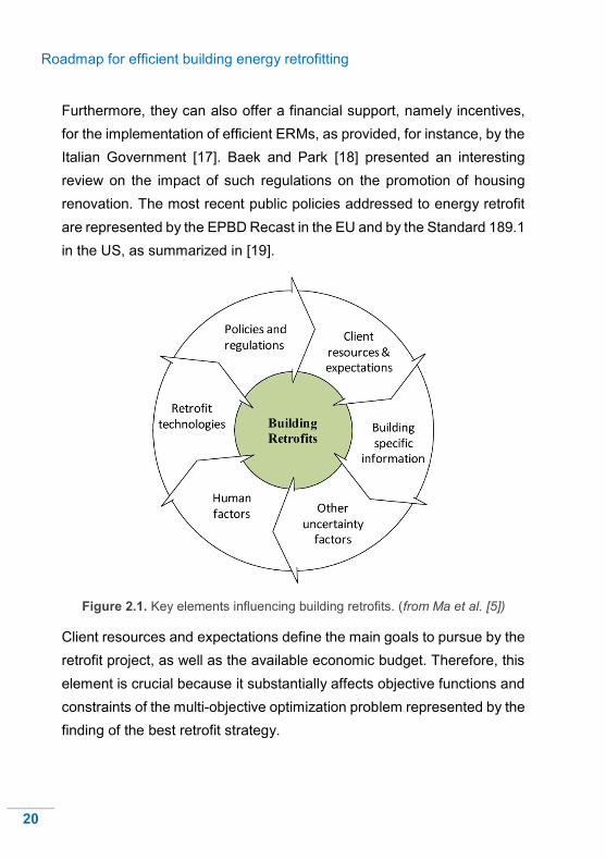
3.3. Application ............................................................................. 50
3.3.1. Presentation of the case study ...................................... 50

Index
2
3.3.2. Results and discussion .................................................. 56
CHAPTER 4. Simulation-based Large-scale uncertainty/ sensitivity
Analysis of Building Energy performance (SLABE) ............................... 70
4.1. Introduction ............................................................................ 70
4.2. Methodology .......................................................................... 72
4.2.1. Stage I. Assessment of energy demand and thermal
comfort (discomfort hours) ............................................................. 75
4.2.2. Stage II. Assessment of primary energy consumption and
global cost ...................................................................................... 78
4.3. Application ............................................................................. 84
4.3.1. Presentation of the case study ...................................... 84
4.3.2. Results and discussion .................................................. 93
CHAPTER 5. Artificial Neural Networks (ANNs) for the prediction of
building energy performance ............................................................... 121
5.1. Introduction .......................................................................... 121
5.2. Methodology ........................................................................ 124
5.3. Application ........................................................................... 130
5.3.1. Presentation of the case study .................................... 130
5.3.2. Results and discussion ................................................ 136
CHAPTER 6. CASA: a new methodology for Cost-optimal Analysis by
multi-objective optimiSation and Artificial neural networks .................. 144
6.1. Introduction .......................................................................... 144
6.2. Methodology ........................................................................ 145
6.3. Application ........................................................................... 147

Index
3
6.3.1. Presentation of the case study .................................... 147
6.3.2. Results and discussion ................................................ 151
CHAPTER 7. Conclusions ............................................................. 161
Nomenclature ...................................................................................... 173
References .......................................................................................... 176

Acknowledgements/ Ringraziamenti
4
Acknowledgements/ Ringraziamenti
I am sorry for my English readers, but this section is in Italian because
my heart is able to speak only the language of my small big Country.
La strada che mi ha portato fino a qui è stata abbastanza lunga; non
è stata facile, ma credo che non sia stata neanche troppo difficile,
perchè il destino è stato spesso dalla mia parte. Ma per destino non
intendo la fortuna che possiede chi vince una scommessa al primo
tentativo (molti possono testimoniare che i tentativi sono stati
parecchi senza ottimi risultati). Il destino mi è stato amico mettendo
tanti amici sul mio cammino, perché, come recita un recente film,
nessuno si salva da solo. Per questo, la lista delle persone che vorrei
ringraziare è lunga, e sono costretto a tagliarla per evitare che sia più
lunga della tesi. Quindi per non scontentare nessuno, inizio con il
ringraziare chiunque stia leggendo queste righe. Se non risulta nella
lista di nomi sottostante, sappia che nella versione completa dei
ringraziamenti è sicuramente presente (vedi allegato in calce, nei
meandri oscuri della mia mente).
Grazie Mamma, Grazie Papà perché mi avete accompagnato in ogni
salita del mio percorso e quando sono diventato troppo pesante per
essere portato in braccio, mi avete dato un bel motorino. Sono fiero di
quello che sono diventato e senza di voi non ci sarei mai riuscito. A
volte provo ad immaginare due genitori migliori di voi.. mi concentro,
ma non ci riesco.
Grazie Roberta, perché la vita è amore, il mio amore infinto sei tu e
quindi tu sei la mia vita. Su quel bel motorino non sono più da solo.
Insieme supereremo ogni curva e salita perché l’amore ha trasformato

Acknowledgements/ Ringraziamenti
5
il motorino in una meravigliosa moto infermabile. A volte provo ad
immaginare la mia vita senza di te.. mi concentro, ma non ci riesco. Ti
amo.
Grazie Gaetano, perché anche se non fossimo fratelli, lo saremmo lo
stesso. Non credo che al mondo esistano molte persone migliori di te
(sicuramente io no). Il bene che provo per te non ha limiti.
PS: Ci tengo a sottolineare che il mio caro fratello ha contribuito a
questa tesi, producendo le figure 2.3 e 5.1.
Grazie Tanino, a cui questa tesi è dedicata. Tanino è mio nonno, non
c’è più ma ci sarà per sempre, perché i grandi uomini non possono
morire. Lui non è un grande uomo.. lui è il grande uomo.
Grazie Prof. (leggi Nicola Bianco), perché ti considero un secondo
padre. Sei un grande prof. non solo in aula universitaria, ma anche
(cosa ben più importante) nella vita. L’amore che provo per il mio
lavoro lo devo a te. E chi ama il proprio lavoro, non lavorerà mai.
Grazie Prof. Giuseppe Vanoli, Grazie Fabrizio, per il supporto
scientifico che mi avete sempre concesso, per i valori umani che mi
avete trasmesso, per l’amicizia che mi avete offerto
Grazie ai miei colleghi, perché tutti hanno colleghi, pochi hanno
colleghi simpatici, pochissimi hanno colleghi-amici, solo io ho colleghi-
amici-autisti (leggi Alessia, Claudio e Filippo). Vi voglio bene.
Grazie ai miei amici di ieri e di oggi, perché la vera amicizia è una
ottimizzazione multi-obiettivo: amplifica le gioie e riduce i problemi.

Acknowledgements/ Ringraziamenti
6
Grazie a tutta la mia famiglia, dai nipotini ai nonni, perché certi valori
basilari si imparano solo con l’esempio. Voi siete un esempio esemplare.
Ringrazio i fautori del progetto POLIGRID - POR Campania FSE
2007/2013: “Sviluppo di reti di eccellenza tra Università-Centri di
Ricerca-Imprese”- per il sostegno finanziario fornito alla mia attività
di ricerca.
Se è vero che il mio cuore parla soltanto Italiano, è altrettanto vero
che molti miei amici ‘olandesi’ non sono tanto pratici della lingua di
Dante. Quindi devo fare uno strappo alla regola:
I want to thank Prof. Jan Hensen and his wonderful research group at
Eindhoven University of Technology, where I spent a very productive
research period, during which worthy outcomes proposed in this thesis
have been achieved (i.e., chapter 4). Special thanks to Jan and my
friend Mohamed Hamdy, great researchers and great persons.
I want to thank my ‘dutch friends’ Alessandro, Angelo, Basar, Davide,
Jonnarella, Marco, Munich, Raffaele, Sami, Yasin because in only six
months we have created a sort of family. You are in my heart.
E’ vero, il destino è stato spesso dalla mia parte, ma in qualche modo
anch’io ho fatto qualcosa per risultare simpatico al destino.
Quindi ringrazio me stesso… per essere precisi, ringrazio il gabbiano
Jonathan che vive dentro di me, sussurrandomi continuamente:
“Non dar retta ai tuoi occhi e non credere a quello che vedi. Gli occhi
vedono solo ciò che è limitato. Guarda col tuo intelletto e scopri quello
che conosci già, allora imparerai come si vola.”

Introduction
7
“Anything else you're interested in is not going to happen
if you can't breathe the air and drink the water.
Don't sit this one out. Do something. Make it sustainable. “
CHAPTER 1. Introduction
1.1. Background
The sustainable development and the effort towards a green, low-carbon
economic represent some of the most crucial challenges of our
generation. The admirable purpose is a better world, in which healthy
environment, economic prosperity and social justice are pursued
simultaneously to ensure the well-being of present and future
generations.
Within this context, the 'Roadmap for moving to a competitive low carbon
economy in 2050’ (EU COM112/2011 [1]) establishes the target of
reducing greenhouse gas emissions by 80–95% by 2050 in comparison
to the levels of 1990. This goal cannot be reached without a substantial
effort for the improvement of building energy performance. Indeed, the
building sector is very energy-intensive – mainly because of the physical
and functional obsolescence of the existing stock – by accounting for
around 40% of primary energy consumption in the European Union (EU)
[2] and 32% in the world [3]. This scenario has generated a great interest
in projecting new nearly zero-energy buildings (nZEBs) in order to reduce
the energy demand of the future building stock. Nevertheless, it is well
known that the building turn-over rate is quite low, especially in the
industrialized countries, which are responsible of a wide part of world
consumption; for instance, most EU states extend their stock by less than

Introduction
8
1% per year [4]. Thus, the impact of the new nZEBs is quite limited,
whereas the energy retrofitting of the existing building stock is a key-
strategy to achieve tangible results in the reduction of energy
consumption and, thus, polluting emissions. However, the path is very
challenging. The renovation rate in the EU, currently around 1%, should
be more than doubled in order to realize, by 2050, a complete
refurbishment of the European building stock [4], which would give a large
contribution to the achievement of the ambitious targets pursed by the
'Roadmap for moving to a competitive low carbon economy in 2050’. It’s
clear that, as perfectly outlined by Ma et al. [5]:
“there is still a long way for building scientists and professionals to go in
order to make existing building stock be more energy efficient and
environmentally sustainable”.
The design of the building energy retrofit is a complex and arduous task,
which requires a holistic and integrated team approach [6], since it
involves two distinct perspectives: the collective (state) one, interested in
energy savings, and the private (single building) one, interested in
economic benefits. How to find out the set of energy retrofit measures
(ERMs) that ensures the best trade-off between such perspectives?
The Energy Performance of Buildings Directive (EPBD) Recast
(2010/31/EU) [7] answers this question, by prescribing the cost-optimal
analysis in order to detect the best packages of energy efficiency
measures (EEMs) to apply to new or existing buildings. More in detail, a
new comparative methodology framework has been introduced to assess
the building energy performance “with a view to achieving cost-optimal
levels”. The recommended package of EEMs is the one that minimizes
the global cost – which takes into accounts both investment and operation
– evaluated over the entire lifecycle of the building, according to the
European Commission Delegated Regulation [8] that supplements the

Introduction
9
EPBD Recast. It should be noted that the proposed thesis is focused on
building retrofitting, because, as aforementioned, this can ensure huge
energy saving potentials. Therefore, the measures for the improvement
of building energy performance are indifferently denoted either with EEMs
or ERMs.
The cost-optimal analysis is a complex procedure that requires numerous
simulations of building energy performance in correspondence of well-
selected combinations of EEMs. In order to obtain reliable results, such
simulations must consider the dynamic behavior of the system over the
year, and thus the use of appropriate building performance simulation
(BPS) tools – e.g., EnergyPlus [9], TRNSYS [10], ESP-r [11], IDA ICE
[12] – is highly recommended. This results in a large amount of the
required computational time that can assume an order of magnitude from
days, for simple buildings, until months, for quite complex ones.
Definitively, because of both high computational burden and complexity
of BPS tools, the assessment of the cost-optimality for every building is a
prohibitive goal, if the standard procedure is adopted. That’s why the
EPBD Recast demands the Member States (MSs) to define a set of
reference buildings (RefBs) in order to represent the national building
stock, and to perform the cost-optimal analysis only on these
representative buildings. The RefBs should cover all the categories of
new and existing buildings, where a category is meant as a stock of
buildings, which share climatic conditions (location), functionality,
construction type. The results achieved for each RefB about the cost-
optimal configurations of EEMs should be extended to the other buildings
of the same category.
The described procedure for the detection of the cost-optimal energy
retrofitting, introduced by the EPBD Recast, yields a series of critical, still-
open questions that have aroused a heated discussion in the scientific

Introduction
10
community. Among them, the main questions, identified in this study, can
be outlined as follows:
q1. How to perform a reliable cost-optimal analysis of the retrofit
measures for a single building?
q2. How to achieve global indications about the cost-optimality of energy
retrofitting the existing building stock?
q3. How to evaluate the global cost of a building with a minimum
computational time and a good reliability?
A definitive and robust answer to these questions is fundamental to
overcome the main obstacle to the large diffusion of the cost-optimal
retrofitting practice. Such obstacle can be summarized in a last crucial
question that includes the previous ones:
q4. How to perform a reliable, fast, ‘ad hoc’ cost-optimal analysis
of the retrofit measures for each building of the stock?
So far, the scientific literature did not propose a full and complete
response to such critical questions.
1.2. Aims and originality
This thesis aims to provide a thorough answer to the aforementioned
questions, by means of an original approach that handles all the issues
involved in a robust and reliable cost-optimal analysis, achievable for
every single building with an acceptable computational burden and
complexity.
Three novel methodologies (CAMO, SLABE, building energy simulation
by ANNs) have been developed for proposing a complete response to the

Introduction
11
first three questions and, then, they are coupled in a macro multi-stage
methodology (CASA) that solves the final fundamental question, which
represents the last step towards a wide-spread cost-optimal building
retrofitting. The methodologies are delineated in the following lines and
schematized in figure 1.1 that highlights the combination and role of
CAMO, SLABE and ANNs inside CASA.
CAMO means Cost-optimal Analysis by the Multi-objective Optimization
of energy performance. This methodology answers to question q1, by
proposing a new procedure for the evaluation of the cost-optimality, by
means of the multi-objective optimization of building energy performance
and thermal comfort. The optimization is performed through the coupling
between MATLAB [13] and EnergyPlus [9], by implementing a genetic
algorithm (GA), and it allows the evaluation of profitable and feasible
packages of energy efficiency measures applied to buildings. Then,
following the adoption of these packages, the global cost over the
lifecycle of the building is calculated in order to identify the cost-optimal
solution.
Compared to the standard approach for cost-optimal analysis, CAMO
allows to consider the thermal comfort in a more rigorous way and to
reduce the computational burden, because a limited number of EEMs,
properly selected by the GA, is explored. Nevertheless, computational
time and complexity are still too high for the application to every building.
This represents the main limit of CAMO.
SLABE means Simulation-based Large-scale sensitivity/uncertainty
Analysis of Building Energy performance. This methodology answers to
question q2, by providing a robust cost-optimal analysis of energy
retrofitting solutions for a building stock. It is based on uncertainty and
sensitivity analysis, carried out by means of MATLAB that handles

Introduction
12
EnergyPlus simulations and outcomes. SLABE explores the effects of
some ERMs on primary energy consumption and global cost related to a
sample of buildings representative of a category. The aim is to detect the
package of measures that represents the cost-optimal solution for most
buildings of the category. The explored retrofit actions include energy
measures for the reduction of energy demand, new efficient HVAC
systems, renewable energy sources (RESs). Furthermore, SLABE allows
to evaluate the effectiveness of current policy of state incentives directed
to such actions and to propose possible improvements.
The main limit of SLABE is the impossibility of obtaining detailed
indications on the cost-optimal ERMs for each single building, because
only global recommendations about the explored category are provided.
ANNs means Artificial Neural Networks, which are surrogate models (or
meta-models), commonly used for ‘subrogating’, i.e., replacing, quite
complex functions. The developed methodology answers to question q3,
by consisting in the adoption of ANNs for the assessment of primary
energy consumption and thermal comfort of each building belonging to a
considered category. Two families of ANNs are generated respectively
for the existing building stock and for the renovated building stock in
presence of ERMs. The ANNs are developed in MATLAB environment,
by using EnergyPlus outcomes as targets for training and testing the
networks. Finally, the created surrogate models can replace the BPS
tools in the evaluation of transient energy performance and, thus, of
global cost, of each building of the considered category, both in absence
and in presence of ERMs. The benefit consists of a drastic reduction of
computational time and complexity. Also the impact of the ERMs on
thermal comfort can be investigated, since this latter is set as a further
output of the ANNs. This allows the possible coupling between CAMO

Introduction
13
and ANNs, which can replace EnergyPlus in the optimization routine.
Different families of networks can be generated for covering all the
categories of the whole building stock, in such a way that the performance
of each building can be assessed with a minimum computational time and
a good reliability. In this way, in the proposed macro-methodology such
surrogate models take place of the RefBs. Indeed, each building category
is no more represented by a reference building but by a family of ANNs.
It is noticed that ANNs are an effective tool, but they are not sufficient for
the cost-optimal analysis, since they need to be implemented in another
methodologies (e.g., CAMO), in which they can ‘subrogate’ the traditional
BPS tools.
CAMO, SLABE and ANNs can be used either as stand-alone procedures
for pursuing the aims summarized, respectively, in the questions q1, q2
and q3 or as stages of the macro-methodology denoted as CASA.
The acronym CASA has a double meaning. On one hand, it expresses
the combination among CAMO, SLABE and ANN. On the other hand, it
refers to the core of the methodology, that is the Cost-optimal Analysis by
multi-objective optimiSation and Artificial Neural Networks. Furthermore,
this appellative has a suggestive meaning, since the Italian translation of
the word ‘casa’ is ‘house’. In the same way as the different components
of a house have different functions but contribute to the ultimate goal,
which is the occupants’ well-being, so CAMO, SLABE and ANN can be
adopted independently for pursuing worthwhile targets, but their
combination in CASA allows to reach the ultimate crucial goal. This is
represented by a reliable, fast, ‘ad hoc’ cost-optimal analysis of the retrofit
measures for each single building. Therefore, CASA provides a thorough
response to question q4, by proposing a multi-stage procedure that can
be applied to each building category and, thus, to each building of the

Introduction
14
stock. More in detail, by referring to an established category, CASA is
articulated in the following stages:
STAGE I. SLABE is implemented to investigate the building category by
detecting the parameters (related to existing stock and energy
retrofit measures) that most affect energy performance and
thermal comfort.
STAGE II. ANNs are developed for assessing thermal comfort, energy
consumption, and thus global cost of the buildings that belong
to the category. The most influential parameters, identified in
stage I, are adopted as Inputs.
STAGE III. CAMO is performed by using the ANNs instead of EnergyPlus
in order to find the cost-optimal package of energy efficiency
measures for any building of the category.
Figure 1.1. Scheme of the proposed methodologies and their coupling for the
cost-optimality of building energy retrofitting: from a single building to stock

Introduction
15
CASA allows to overcome the main aforementioned limits of CAMO,
SLUSABE and ANNs, by providing a powerful tool for a reliable and fast
cost-optimal analysis of every building.
1.3. Organization of the thesis
After the present Introduction (chapter 1) and before the Conclusions
(chapter 7), the thesis is articulated in the following chapters:
CH. 2. A roadmap for efficient building retrofitting is proposed, by focusing
on the state-of-art of scientific literature in such field and on the
guidelines of EPBD Recast [7, 8] for identifying cost-optimal ERMs.
CH. 3. The state of art in the field of simulation-base optimization of energy
performance is presented. Then, CAMO is detailed, and applied to a
residential existing building located in Naples (South Italy).
CH. 4. The state of art related to the implementation of uncertainty and
sensitivity analysis in the study of building energy behavior is
presented. Then, SLABE is detailed, and applied to a specific
category: office buildings built in South Italy in the period 1920-1970.
This building category is considered also in the next two chapters.
CH. 5. The state of art related to the adoption of surrogate models in the
analysis of building energy performance is presented. Then, the
ANNs methodology is detailed, and applied to the cited category.
CH. 6. CAMO, SLABE and ANNs are combined inside CASA, which is
described in detail, and applied to a building of the cited category.
It’s noted that the description of each methodology is followed by the
application to a case-study, which acts as a sort of validation procedure.

Roadmap for efficient building energy retrofitting
16
“Energy efficiency is the most
powerful renewable source”
CHAPTER 2. Roadmap for efficient building energy retrofitting
2.1. Introduction
In recent years, a great effort has been made, at international level, for
reducing the energy consumption of buildings. Indeed, the construction
sector represents one of the main challenges to deal with in order to
guarantee a sustainable development for our sons and, more in general,
compatible with a suitable common future.
At the European level, starting from 2002, with the entrance into force of
the EPBD (Energy Performance of Building Directive – 2002/91/CE [14]),
for the first time in the history, all Member States of an entire continent
decided to establish common guidelines for improving the energy
performance of buildings, concerning both new and existing
architectures. In this regard, at national level, several laws have been
formulated for receiving the European mandatory trends, by taking into
account the local peculiarities of the building stock, technology and
construction activities.
Some years later, the EPBD Recast (2010/31/EU [7]) has been enacted.
Really, this was only a further step of a continuous process aimed at
reducing, with targets increasingly more ambitious, the impact of human
activity on climate change. This Directive introduces the goal of nearly
zero-energy buildings (nZEB), by underlining both the high-required
performance as well as the economic feasibility of the ‘building system’,

Roadmap for efficient building energy retrofitting
17
by means of the new concept of cost-optimality. In this respect, the EPBD
Recast establishes that the Member States (MSs) have to define local
regulations in order to fulfil the standard of nearly zero-energy building:
starting from January 2021, for all new buildings;
starting from January 2019, for new buildings owned and/or occupied
by public administration and public authorities.
As it is clear, we are talking of a very near future.
Diversely from the net zero-energy building (NZEB), a nZEB has not an
established energy performance to satisfy. More in detail, as specified in
the EPBD Recast, it is “a building that has a very high energy
performance. The nearly zero or very low amount of energy required
should be covered to a very significant extent by energy from renewable
sources, including energy from renewable sources produced on-site or
nearby”. However, such definition is quite vague. Globally, a nearly zero-
energy building should ensure higher energy performance compared to
the cost-optimal configuration of the building.
In spite of the importance of new green and efficient buildings, the energy
refurbishment of existing buildings offers much larger opportunities for
reducing energy consumption and polluting emissions, as argued in the
Introduction of this thesis.
In light of this, the EU guidelines establish that a great attention should
be given to the energy retrofit of existing buildings. More in detail, the
EPBD Recast and the delegated regulation N. 244/2012 of the European
Council [8] introduce the cost-optimal analysis for assessing the most
effective packages of energy retrofit measures (ERMs); this procedure is
detailed in section 2.3, since it is adopted in the next chapters.
Furthermore, the EU Directive 2012/27/EU [15], underlines the necessity,
for all MSs, to support “a long-term strategy for mobilizing investment in
the renovation of the national stock of residential and commercial

Roadmap for efficient building energy retrofitting
18
buildings, both public and private”. In this regard, the Directive promotes
“cost-effective approaches to renovations, relevant to the building type
and climatic zone” as well as “policies and measures to stimulate cost-
effective deep renovations of buildings, including staged deep
renovations". Moreover, the same document suggests “an evidence-
based estimate of expected energy savings and wider benefits". In this
frame, the public role should be exemplary, since “each Member State
shall ensure that, as from 1 January 2014, 3% of the total floor area of
heated and/or cooled buildings owned and occupied by its central
government is renovated each year to meet at least the minimum energy
performance requirements”.
A great effort for improving the energy performance of the existing
building stock has been made also at international levels. This is shown
by the number of Annex projects, developed by the International Energy
Agency (IEA) in recent years, for promoting the energy efficiency of
existing buildings, such as:
Annex 46 – Holistic assessment tool kit on energy efficient retrofit
measures for government buildings;
Annex 50 – Prefabricated systems for low energy renovation of
residential buildings;
Annex 55 – Reliability of energy efficient building retrofitting;
Annex 56 – Energy & greenhouse gas optimized building renovation
[16].
These projects provided policy guidance, financial and technical support
for the implementation of ERMs. As highlighted by Ma et al. [5], building
energy retrofitting offers many challenges and opportunities. The
substantial challenges, in any sustainable refurbishment project, are due
to the presence of several uncertainties, such as climate change, human
behavior, state policy, which have a large impact on the project success.

Roadmap for efficient building energy retrofitting
19
Furthermore, the building is a very complex system, consisting of highly
interactive components. Therefore, the evaluation of the effects induced
by ERMs on the building behavior is much critical, and the selection of
the best retrofit strategy becomes very complex. Indeed a rigorous
approach generally requires the solving of a multi-objective optimization
problem (see chapter 3). On the other hand, the huge opportunities,
provided by an efficient energy retrofitting of the existing stock, involve
the reduction of pollution, operating cost and maintenance needs as well
as increment of thermal comfort and an improvement of national energy
security.
2.2. State of art
The scientific community supports the necessity of acting on the existing
stock, in order to promote a drastic reduction of energy consumption and
green-house gas emissions of the building sector. In this regard, the
current literature provides a large number of studies on the huge
potentials of building energy refurbishment.
2.2.1. Key elements for an efficient energy retrofit
In an admirable effort, Ma et al. [5] proposed a detailed review and
analysis of the main methodologies adopted for designing an efficient
energy retrofit, thereby identifying some key elements. Figure 2.1, which
is taken from the referred-to study, depicts such elements that consist of:
policies and regulations, client resources and expectations, building
specific information, human factors, retrofit technologies and other
uncertainty factors.
Renovation policies and regulations impose the minimum levels of energy
performance that should be achieved in case of refurbishment.
Roadmap for efficient building energy retrofitting
20
Furthermore, they can also offer a financial support, namely incentives,
for the implementation of efficient ERMs, as provided, for instance, by the
Italian Government [17]. Baek and Park [18] presented an interesting
review on the impact of such regulations on the promotion of housing
renovation. The most recent public policies addressed to energy retrofit
are represented by the EPBD Recast in the EU and by the Standard 189.1
in the US, as summarized in [19].
Figure 2.1. Key elements influencing building retrofits. (from Ma et al. [5])
Client resources and expectations define the main goals to pursue by the
retrofit project, as well as the available economic budget. Therefore, this
element is crucial because it substantially affects objective functions and
constraints of the multi-objective optimization problem represented by the
finding of the best retrofit strategy.

Roadmap for efficient building energy retrofitting
21
A further key element for an effective retrofit is the exploitation of building-
specific information, such as geographical location, geometry, size, age,
intend use, occupancy profiles, operation schedules, energy sources,
type of HVAC system and so on. This information should be considered
in order to propose the most appropriate ERMs.
Human factors constitute another relevant element for the success of the
refurbishment. They involve the occupants’ behavior, in terms of comfort
needs, activity schedules, and access to controls, thereby implying a
deep influence, characterized by a significant uncertainty, on the final
outcomes of a retrofit project [20]. Several studies showed that a proper
and smart occupants’ behavior can produce substantial energy savings,
with no or low investment and without penalizing thermal comfort. For
instance, Owens and Wilhite [21] demonstrated, for Nordic countries, a
saving of domestic energy use until 20%, while Santin et al. [22] showed
that the impact of people behavior on the energy use for heating is close
to 5% in the Netherlands.
The retrofit technologies correspond to the energy retrofit measures
(ERMs). They represent renovation actions aimed at the reduction of
building primary energy consumption. In their paper, Ma et al. [5]
proposed a possible classification of the retrofit measures in three
categories – depicted in figure 2.2 (taken from the mentioned study) –
consisting of:
a) supply side management;
b) demand side management;
c) change of energy consumption patterns.
The category a) includes the implementation of efficient primary heating/
cooling systems as well as of renewable energy sources (RESs), such as
thermal solar collectors, photovoltaics (PV) generators, wind turbines,
biomass systems, and so on. The purpose is providing the building with

Roadmap for efficient building energy retrofitting
22
innovative and efficient energy supply systems. In recent years, the
interest in RESs is more and more increasing, mainly because of the
rising concern to environmental issues and of the decreasing investment
cost for such systems, also thanks to very favorable national policies of
financial support. The use of renewables, above all PV generators, can
be particularly effective for office buildings, by virtue of the high electricity
demand. This observation is proved in this thesis, by the outcomes
proposed in chapter 4.
Figure 2.2. Main categories of building retrofit technologies. (from Ma et al. [5])
The category b) (demand side management) collects different energy
measures for the reduction of heating and cooling demand, such as the
renovation of the building fabric, efficient windows, solar shading
systems, natural ventilation, heat recovery, thermal storage systems, and
many other efficient technologies.
The category c) (energy consumption patterns) considers the ERMs,
generally with no or low investment cost, that point to properly address

Roadmap for efficient building energy retrofitting
23
the human factors. In fact, as aforementioned, a smart and appropriate
occupants’ behavior can induce high energy savings, until 20%.
A further crucial issue for the success of energy retrofitting strategies
concerns the reliable and accurate estimation of the building energy and
thermal performance. This is fundamental in order to faithfully assess the
impact of the proposed ERMs on energy consumption and thermal
comfort, thereby providing all the energy and economic indicators – e.g.,
saving of energy demand, pay-back period, global cost – required for
identifying the best solution. Therefore, simple steady-state methods are
inadequate, whereas the recommended choice is the adoption of proper
BPS tools that perform reliable dynamic energy simulations. There are
several whole building energy simulation programs, such as EnergyPlus,
TRNSYS, ESP-r, IDA ICE that provide an accurate investigation of the
energy effects induced by the considered retrofit measures. These
programs are widely used in the scientific community, because of their
high capability. However, the development of whole building energy
models is, generally, a complex task, which requires the calibration with
experimental data for achieving a robust accuracy. Hence, also other
methods can be used for estimating the energy and thermal benefits
produced by retrofit measures. In this regard, Richalet et al. [23]
delineated three approaches for assessing building energy performance,
consisting of: the computational-based approach by means of BPS tools,
calibrated through data deriving from energy audits; the performance-
based approach, founded on exploiting the information coming from
building utility bills; the measurement-based approach, founded on in-situ
experimental measures. On the same track, Poel et al. [24] proposed an
overview of the most popular methods and programs for the energy
analysis of existing dwellings. Several software and tools are available,

Roadmap for efficient building energy retrofitting
24
thus the best choice, for a specific project, is not trivial and depends on
different factors, such as client requirements, required level of accuracy,
available time and budget and so on.
2.2.2. Worthy retrofit studies
Ma et al. [5] also proposed a detailed review of worthy studies provided
by the current scientific literature in the field of building energy retrofitting.
Such studies are subdivided in two groups: those focused on residential
buildings and those focused on commercial office buildings. This
distinction is made because the best ERMs for heterogeneous building
types and uses, e.g., dwellings vs offices, generally differ, as also shown
in this thesis that investigates two different case-studies related to the
mentioned categories: CAMO is applied to a residential building (chapter
3), whereas SLABE, ANNs and CASA are tested on office buildings
(chapters 4, 5, 6). It is noticed that the attention is directed to these two
categories because they cover the vast majority of the building stock of
any country.
In the following lines, some worthy retrofit studies belonging to the
referred-to groups are briefly described. For a deeper overview of the
current state-of-art the reader is invited to refer to [5].
Residential buildings
The energy retrofitting of the residential sector assumes a fundamental
role, because a large part of the building stock is composed of dwellings.
For instance, in Italy there are 13.6 million of buildings, of which 11.7
million (more than 87%) are residential buildings [4]. Furthermore,
concerning this category, as shown by Nemry et al. [25] at the EU level,
the potential reduction of the environmental impact of new buildings can

Roadmap for efficient building energy retrofitting
25
be neglected compared to that of existing ones. Thus, an efficient energy
retrofitting policy assumes a huge importance.
Some interesting studies are focused on the investigation of ERMs for the
reduction of heating and cooling demand (demand side management).
On this track, Cohen et al. [26] explored the effectiveness of individual
ERMs, thereby concluding that, generally, the insulation of the opaque
building envelope is convenient, while the windows replacement isn’t,
because of the small normalized annual energy saving. However, this
conclusion is valid only for heating-dominated climates (e.g., Northern
Europe), whereas in presence of cooling-dominated climates (e.g.,
Mediterranean area) a deeper analysis is required in order to take into
account that the issue of overheating in summertime. The selection of
retrofit measures, aimed at a good trade-off between heating and cooling
needs, is deeply examined in section 2.2.3. Stovall et al. [27] carried out
an experimental analysis for exploring different wall retrofit options,
thereby finding that that the external insulant sheathing exercises a high
influence in the reduction of the heat transfer through the wall. Nabinger
and Persily [28] considered an unoccupied house for exploring the impact
different ERMs for improving the building air-tightness on ventilation rates
and energy consumption.
Other worthwhile studies are focused on the investigation of ERMs
addressed to the supply side management, by the adoption of efficient
energy conversion systems and RESs. Hens [29] studied a two-storey
house built in 1957, showing that the benefits induced by solar thermal
and PV panels are minimal compared to the adoption of higher levels of
thermal insulation, energy efficient windows, improved ventilation, and
central heating. Goodacre et al. [30] performed a cost-benefit analysis of
retrofit measures aimed at improving the primary heating and DHW

Roadmap for efficient building energy retrofitting
26
systems in the English housing stock; they highlighted the high influence
of uncertainty. Boait et al. [31] investigated the installation of domestic
ground source heat pumps (GSHPs) in UK dwellings; they showed that
the seasonal performance of such efficient system, highly affected by the
time constant of the building, was worse compared to that estimated in
other European studies.
Recently, Kuusk et al. [32] proposed a detailed study on the energy
retrofitting of brick apartment buildings in Estonia (cold climate). Most
notably, they examined the energy usage of such dwellings by performing
simulations for four reference building types, representative of the stock.
The outcomes showed that the energy renovation of old apartment
buildings can allow to reach the same energy performance requirements
as in new apartment buildings. On the same track, Dodoo et al. [33]
analyzed the retrofit of a four-storey wood-frame apartment to a passive
house and Xing et al. [34] proposed a hierarchical path towards zero
carbon building refurbishment, based on the improvement of the building
envelope thermal characteristics, the use of more efficient building
equipment, and micro generation.
The last mentioned studies show that the energy retrofit of existing
buildings to passive, low, nearly zero-energy buildings is possible in cold
climates. Nevertheless, it is much more complicated in warm (cooling-
dominated) climates, because contrasting phenomena are generated by
the ERMs, as outlined in section 2.2.3. Furthermore, in most cases, a
similar extreme energy retrofit strategy is not cost-effective, also in
heating-dominated climates. That’s why the EPDB Recast has introduced
the concept of cost-optimality.

Roadmap for efficient building energy retrofitting
27
Commercial office buildings
The main peculiarity of office buildings, compared to dwellings, is
represented by a higher demand for lighting and various electric uses, as
well as by a much larger endogenous heat gain that increases the energy
demand for space cooling. Therefore, also in heating-dominated climates,
the main components of annual primary energy consumption, i.e., space
heating, space cooling, lighting, electric equipment, are more balanced
compared to residential buildings, whose consumption is highly affected
by space heating. This determines major issues in the design of the
refurbishment strategy.
Indeed, as outlined by Rey [35], office building energy retrofitting is
influenced by a large number of parameters, thereby implying the
necessity of a structured multi-criteria approach, which simultaneously
should take into account environmental, sociocultural and economic
criteria. In the same vein, Roulet et al. [36] developed a multi-criteria
rating methodology, denoted as Office Rating MEthodology (ORME), in
order to rank retrofit scenarios according to energy demand for heating,
cooling and other appliances, environmental impact, indoor comfort and
cost. Arup [37] proposed a detailed guide for the refurbishment of existing
office buildings, through a six-step plan, consisting of: determining the
baseline, establishing goals, reviewing building maintenance,
housekeeping and energy purchase strategy, crunching time: establish
or demolish, selecting the optimal ERMs and getting started.
The implementation of whole building retrofits for commercial buildings
was discussed by Olgyay and Seruto [38] and Fluhrer et al. [39], who
compared the adopted approach with the typical retrofit approach
commonly used by ESCOs, thereby obtaining an increase of energy
saving of around 40%. Hestnes and Kofoed [40] investigated ten existing

Roadmap for efficient building energy retrofitting
28
office buildings, by exploring the impact of different retrofit strategies,
including measures addressed to building envelope, HVAC system and
lighting. The outcomes confirmed the complexity of designing energy
retrofit for the considered building category, since the optimal strategy
significantly depends on the very specific building energy characteristics.
The effectiveness of multiple ERMs on the energy consumption of office
buildings was also examined by Chidiac et al. [41]. Dascalaki and
Santamouris [42] investigated the potentials of energy saving induced by
well-selected ERMs for five office building types in four different European
climatic zones. The retrofit measures included the improvement of
building envelope, HVAC system, artificial lighting systems, and the
integration of passive components for heating and cooling. Cooperman
et al. [43] argued that the renovation of the building fabric, mainly oriented
to the adoption of efficient windows, is a key action for improving the
energy performance of commercial buildings. In the same vein, Chow et
al. [44] showed that an energy conservation up to 40% can be achieved
by means of a retrofit strategy directed to the building enclosure, for
existing public buildings in China.
However, these outcomes are not valid for any climate. Indeed, for
cooling-dominated climates, the improvement of HVAC system efficiency
ensures huger potentials of energy savings compared to retrofit
measures on the envelope. This is proved in the chapter 4 of this thesis.
Barlow and Fiala [45] showed how the application of adaptive thermal
comfort theories could play an important role for future refurbishment
strategies for existing office buildings.
Finally, different interactive decision support tools have been designed
[46-48] for quickly identifying optimal energy retrofit measures in office
buildings, on the basis of the trade-off among different performance

Roadmap for efficient building energy retrofitting
29
indicators, such as investment cost, improved building performance, and
environmental impacts.
2.2.3. The trade-off between heating and cooling needs
For both reasons of indoor comfort and limitation to the use of energy
systems, a new issue, mainly in cooling-dominated climates (as the
Mediterranean one), has to be considered. In this regard, a too high level
of thermal insulation, as required by the recent regulations, can lead to a
substantial increase of the energy demand for cooling in summertime,
because of the phenomenon of indoor overheating. Therefore, the proper
choice of the envelope thermal resistance should be made contextually
to overall evaluations and other parameters, such as the annual energy
performance, the thermal capacity of the building thermal envelope, the
radiative characteristics of external coatings. Moreover, the potential of
indoor free cooling, mainly during nighttime, should be carefully
investigated by considering various heat transfer phenomena, and thus
the emission to the sky and to the external environment, and/or the
nocturnal ventilation, preferably natural in order to avoid the electricity
demand of fans. All told, the combined effects of insulation, thermal
capacity, radiative behaviors of the surfaces, free cooling, climatic
conditions and building use have to be explored. A primary role is played
by the building envelope, which has to mitigate the heat transfer between
the external environment and the internal one, due to the high external
temperatures during the central hours of the day and, above all, due to
the solar radiation. This latter highly affects the cooling load, because: a)
it is incident on the external surface (and thus rises the sol-air
temperature), b) enters into the environment directly through the
windows, c) is reflected into the building because of the reflection of the

Roadmap for efficient building energy retrofitting
30
surrounding elements. By means of the selection of proper levels of
thermal insulation and thermal capacity of the envelope, appropriate
external coatings for optimizing the sol-air temperature (which affects the
heat transfer through the opaque structures), window shadings and
controls, an effective design of the building shell can give a huge
contribution in improving the building thermal performance. Really, when
the target is, beyond the thermal comfort, the achievement of low energy
buildings from a point of view of the global performance (heating, cooling,
lighting and other uses), the best compromise among the aforementioned
characteristics should be found out. In this regard, some choices can
have contrasting effects, for instance:
too high levels of thermal insulation, even if surely beneficial during
the heating season, can induce phenomena of indoor overheating in
summer. Indeed, when solar gains and endogenous loads are
significant, low values of the envelope thermal transmittance can
deprecate the useful heat losses (heat dissipation), also during the
nighttime, so that a common hyper-insulation phenomenon occurs;
high levels of thermal capacity can provide useful time lags and
attenuation of the heat wave transferred between the external and
internal environments. Nevertheless, they can also imply a long inertia
of the indoor environment for reaching the desired temperatures when
the HVAC system is turned on (mainly if with radiant terminals).
highly reflective coatings, even if suitable for keeping cool the outer
building surfaces (by reducing the sol-air temperature), can yield too
cold surfaces in wintertime, above all in presence of high values of
thermal emissivity that can cause a significant cooling of the building
shell, because of the radiative heat transfer with the surrounding
environment and the sky (during nighttime).

Roadmap for efficient building energy retrofitting
31
Of course, the windows exercise a substantial influence on the building
energy performance. Indeed, their thermal transmittance highly impacts
on the heat transfer phenomena through the envelope. Furthermore, the
adoption of different coatings (low emissive, reflective, selective and so
on) and/or different shading systems (internal, external, managed by
manual operation or based on the incident solar irradiance) greatly
affects, in all seasons, the amount of favorable (heating season) or
penalizing (cooling season) solar gains.
All told, in presence of temperate/ warm climates, a deep care is
fundamental in defining the best solutions for optimizing the behavior of
the envelope. Indeed, diversely from the consolidated approach for cold
climates, where the main need is the reduction of energy demand for
space heating, a different design activity is required in warm climates
because of the aforementioned contrasting phenomena. In this regard, a
very interesting study was carried out by Kolokotroni et al. [49], who
investigated the indoor overheating in summertime, by also considering
climate projections for the next years. Jenkins et al. [50], on the same
track, developed a surrogated model, by integrating dynamic energy
investigations and probabilistic climate forecasts for the future. Recently,
worthwhile studies of Santamouris and Kolokotsa [51, 52] and
Santamouris et al. [53] discussed the impact of the progressive
overheating of urbanized areas on the energy demand and health
conditions in civil European buildings. The attention towards the next
decades has been evidenced also by Porritt et al. [54], who highlighted
how the progressive increasing frequency of extreme weather events
could affect the indoor comfort in residential buildings of the United
Kingdom. The authors showed that measures for managing solar gains
and external insulation of the envelope can be effective. On the other

Roadmap for efficient building energy retrofitting
32
hand, thermal insulation, placed on the internal side, can increase the
indoor overheating phenomenon during the warm season.
Really, as evidenced by Ascione et al. [55] for various European climates,
the right combination of insulation, thermal mass and radiative
peculiarities of the external coatings depends on both climate and
potentials of summer free cooling by means of ventilation. In this regard,
beyond the thermal mass, even new technologies, for instance based on
the adoption of phase change materials (PCMs), can be successfully
adopted [56], even if the costs have to be carefully evaluated.
In general, two macro-strategies can be identified for reducing the cooling
need and improving, at the same time, the thermal comfort during the
warm season:
a) the reduction of the heat gains that, instantaneously or shifted,
become cooling load;
b) the adoption of techniques for discharging the building envelope and
operate a passive cooling of the indoor spaces.
With reference to the point a), the use of solar shadings and their
effectiveness [57, 58] as well as the adoption of reflective coatings [55,
59], also by taking into account the interrelation among buildings [60, 61],
have been largely studied in recent years by authoritative authors. In
particular, Bellia et al. [57] investigated the suitability of various kinds of
windows’ screens, for several climates, while Katunský and Lopušniak
[58] analyzed the influence of shading systems on cooling demand and
on the phenomenon of indoor overheating in low-energy buildings. About
cool colors and cool paints, Ascione et al. [55] proposed an index for
orienting the choice of solar reflectance and thermal emissivity deepening
on winter degree-days and solar irradiance in summertime. Furthermore,
Cotana et al. [59] evaluated how the albedo of the building envelopes, at
urban scale, can contribute in reducing the global warming. Some of the

Roadmap for efficient building energy retrofitting
33
same authors, in previous works [60, 61], analyzed what happens
because of the mutual reflection among buildings.
With reference to the point b), a wide review has been recently proposed
by Kamali [62], who discussed the potentiality of PCMs in reducing the
cooling load of buildings. Diversely, Inard et al. [63] verified the free
cooling potential of natural ventilation in low-energy office buildings.
Really, free cooling represents a powerful technique for improving the
building energy performance in summertime, without penalizing the
heating season, as investigated also by Shaviv et al. [64] and Cheng and
Givoni [65].
Finally, we can conclude that the design of building energy retrofitting is
a critical task that requires a multi-objective approach because of the
presence of contrasting targets, subject to several constraints, related to
building characteristics and economical considerations. The optimal
solution is a trade-off among energy related and non-energy related
objectives, such as the minimization of energy consumption, thermal
discomfort, investment cost, polluting emissions and so on. The EPBD
Recast condenses most of these targets in the concept of cost-optimality.
2.3. Cost-optimality
As already mentioned, the EPBD Recast [7] introduces the cost-optimal
analysis for detecting the best EEMs to apply to new or existing building
“with a view to achieving cost-optimal levels”. More in detail, he EU
Commission Delegated Regulation n. 244/2012 [8], supplements the
Directive, by establishing a “comparative methodology framework for
calculating cost-optimal levels of minimum energy performance
requirements for buildings and building elements”. The cost-optimality is
an innovative and powerful concept that ensures the best trade-off

Roadmap for efficient building energy retrofitting
34
between the two distinct perspectives involved in the building world: the
collective (state) one, interested in the reduction of energy consumption
and polluting emissions, and the private (single building) one, interested
in the reduction of economic disbursement.
The cost-optimal analysis should be applied to the design of both new
buildings and energy retrofits. In any case, it allows to identify ‘best’
packages of energy efficiency measures (EEMs) that minimize the global
cost over the entire lifecycle of a building. The global cost takes into
account investment costs, replacement costs and operating costs and
should be calculated according to the procedure delineated in the
mentioned delegated regulation. More in detail, the cost-optimal analysis
requires to compare the global cost (GC) and the primary energy
consumption (PEC) in correspondence of different packages of EEMs.
Such measures should range from those in compliance with current
regulations to those required by nZEBs, thereby including RES systems.
The final outcome is a predicted cost-optimal curve that depicts the value
of GC (ordinate) in function of PEC (abscissa) for all the investigated
combinations of commonly used and advanced EEMs, as shown in figure
2.3. This curve presents a minimum that identifies the cost-optimal
package of energy efficiency measures. The part of the curve to the right
of the cost-optimality represents solutions that underperform in both
environmental and financial aspects. Diversely, the part of the curve to
the left identifies low and nearly zero-energy buildings. Finally, the figure
shows the distance to the target of nZEBs prescribed by the EPBD Recast
for new buildings, starting from 2021.
This kind of analysis cannot be applied to each single building for reasons
of computational complexity and, therefore, a set of reference buildings
(RefBs) must be defined [8] in order to represent the national stock [66].

Roadmap for efficient building energy retrofitting
35
This approach has been already proposed in many studies, such as the
one of the BPIE for Germany, Poland and Austria [67], but also in recent
scientific papers, concerning the design of new buildings [68, 69] or the
refurbishment of existing ones [70, 71].
Figure 2.3. Cost-optimal curve
The detection of cost-optimal levels and nZEB solutions is an arduous
task, since it requires to explore a huge number of design solutions
(combinations of EEMs). Therefore, the adoption of optimization
procedures is highly recommended, as shown in the next chapter.

Cost-optimal Analysis by Multi-objective Optimization (CAMO) of building energy performance
36
How to perform a reliable cost-optimal analysis
of the retrofit measures for a single building?
CHAPTER 3. Cost-optimal Analysis by Multi-objective Optimization (CAMO) of building energy performance
3.1. Introduction
The cost-optimal analysis prescribed by the EPBD Recast for the
detection of the ‘best’ energy efficiency measures (EEMs) for new or
existing buildings is a complex task. Indeed, how can the cost-optimal
technologies be detected? Moreover, how can the most proper packages
of EEMs be chosen in order to obtain the cost-optimality? This chapter
aims to solve such issues, by proposing CAMO, a new methodology for
performing the Cost-optimal Analysis by means of the Multi-objective
Optimization of energy performance and thermal comfort.
After the coming into force of the EPBD Recast, the scientific community
involved in building energy modeling is animated by a new crucial
discussion, concerning the modalities for performing the cost-optimal
study in order to have rigorous outcomes. Surely, suitable optimization
methods, based on energy simulations and aimed at tailored and reliable
evaluations of the energy performance of buildings, are a possible
solution [72]. The designers often adopt building performance simulation
(BPS) tools for analyzing the energy behaviors of buildings, as well as for
achieving specific scopes, like – for instance – the reduction of the energy
request or the improvement of indoor comfort. In order to improve the
energy performance of buildings, one of the first developed approaches

Cost-optimal Analysis by Multi-objective Optimization (CAMO) of building energy performance
37
has been the ‘parametric simulation method’. This approach makes
variable, within a proper range, some design parameters, in order to see
their effects on some objective functions, while other variables are
constant. Under the point of view of computation, this method is very
expensive and not completely reliable because of the non-linear
interactions among the design variables. Therefore, starting from the
1990s, numerical optimizations and/or simulation-based optimizations
[73] are being adopted more and more frequently, also thanks to the very
rapid diffusion of the computer science. A numerical optimization
methodology can be defined as an iterative procedure that provides
progressive improvements of the solution until the achievement of a sub-
optimal configuration (the ‘actual optimal’ is normally unknown) [74-76].
In the last years, many studies focused on the combination of BPS tools
and optimization programs, in order to improve the optimization
algorithms, above all for reducing the required computational time and
CPU resources. Presently, several algorithms are available, typically
classified like local or global methods, heuristic or meta-heuristic
methods, derivative-based or derivative-free methods, deterministic or
stochastic methods, single-objective or multi-objective algorithms and
many more. The research community involved in the topic of building
energy performance often prefers the use of derivative-free optimization
routines [77], because a continuous or differentiable objective function
does not exist and the gradient information, even if obtained numerically
from the model, is not accurate in many cases. With reference to the
derivative-free methods, genetic algorithms (GAs) are the most popular.
Indeed, these concern a class of mathematical optimization approaches
which reproduce the natural biological evolution, as long as the processes
of inheritance, selection, mutation and crossover provide an optimal
population after a number of iterations (generations). Genetic algorithms

Cost-optimal Analysis by Multi-objective Optimization (CAMO) of building energy performance
38
have had a good diffusion in the building simulation community, because
these can manage black box functions as those provided by BPS tools.
Moreover, these methods have a quite low probability of converging to
local minima, without ensuring the optimal solution, but producing a good
solution (sub-optimal), close to the optimal one, in a reasonable time.
Furthermore, with reference to the building sector, GAs allow multi-
objective optimizations that are more appropriate compared to the single-
objective ones. Indeed, generally, there are conflicting goals at the same
time. Therefore, high performance buildings require a holistic and
integrated team approach [6]. Even with well-coordinated researches, it
is difficult to find a meeting point that allows the optimal solution for all
necessities. Thus, the multi-objective optimization is generally required in
building applications. The main purpose is to identify the so-called ‘Pareto
front’, and thus the set of non-dominated solutions. With reference to the
building efficiency, in order to avoid too complex problems, the
researchers usually define only two objective functions to minimize, such
as carbon dioxide equivalent emissions and investment cost [78], carbon
dioxide equivalent emissions and life cycle cost [79], energy demand and
thermal discomfort [71, 80-83]. In few cases, some studies propose the
minimization of three functions, like energy demand, carbon dioxide
equivalent emissions, investment cost [84], or energy demand, thermal
discomfort and investment cost [85].
CAMO is a new methodology for performing the cost-optimal analysis of
EEMs, suitable for the application to new or existing buildings, on which
the present thesis is focused. In detail, CAMO provides the multi-objective
optimization of energy demand and thermal comfort. The optimization
procedure implements a GA and is based on the combination between
EnergyPlus and MATLAB. As shown in the following sections, after the
presentation of the coupling strategy, the methodology is used for

Cost-optimal Analysis by Multi-objective Optimization (CAMO) of building energy performance
39
assessing the cost-optimal energy retrofitting of an existing building
located in the Italian city of Naples (Southern Italy, Mediterranean
climate). The correspondent IWEC weather data file (available at [86]) is
used in the energy simulations.
It is recalled that CAMO can be adopted either as a stand-alone
methodology for the investigation of a single building or as a part (stage
III) of the macro-methodology (CASA) proposed in this thesis (see
chapter 6).
3.2. Methodology
The new approach, based on the multi-objective optimization, is proposed
for the evaluation of the cost-optimal solution with reference to the energy
refurbishment of existing buildings. Analogously, CAMO is suitable also
to be applied to new buildings, by considering RefBs. The method
combines EnergyPlus and MATLAB. EnergyPlus has been chosen like
BPS tool for two main reasons: a) on one hand, this program allows
reliable modeling of both building and HVAC systems, and, secondly, b)
it works with text-based inputs and outputs, and these facilitate the
interaction with optimization algorithms. According to [73], EnergyPlus is
probably the most widely “whole building energy simulation program” [9]
used for the research in matter of building optimization. A number of
studies testify its reliability in predicting energy performance of buildings
and facilities. Obviously, a proper definition of the models and expertise
in the assignment of all boundary conditions (starting from the selection
of the solution algorithms of the heat transfer) are required. Analogously,
with reference to the optimization ‘engine’, MATLAB has been chosen for
the following two main reasons: a) the program has a very strong
capability, which enables the multi-objective optimization by means of

Cost-optimal Analysis by Multi-objective Optimization (CAMO) of building energy performance
40
GAs and, moreover, b) this can automatically launch EnergyPlus as well
as manage files of both input and output.
The methodology, fully described in the following paragraphs, like a
generic optimization process [73], can be subdivided in three main
phases: 1) pre-processing phase, 2) optimization phase and 3) multi-
criteria decision making phase.
3.2.1. Pre-processing
The combination of BPS tool and optimization program is here developed
and structured, by defining also the formulation of the optimization
problem. That phase is very significant, because this concerns the
boundaries between building science and mathematical optimization, by
requiring a satisfactory expertise in both the fields. Initially, the existing
building or the reference building (i.e., in case of new constructions) is
defined in EnergyPlus, both with reference to the thermal envelope and
the HVAC system, by means of the creation of a text-based format input
file (.idf). Then, the parameters that most affect the energy performance
are identified like design variables. This selection can be performed after
a proper sensitivity analysis [87] or can be derived from a detailed study
of the system. However, it requires a satisfactory expertise in matter of
energy efficiency in buildings.
The value assumed by each variable corresponds to design decisions
and these concern the envelope (e.g., insulation thickness, type of
windows), the heating and cooling systems (e.g., kind of heat emitters,
boilers, chillers) or the operation (e.g., usage of the building, defined
through a set of schedules). Examples of schedules are the set points of
indoor temperatures for both heating and cooling or the definition of the
hourly profiles of the building occupancy along the year. Some

Cost-optimal Analysis by Multi-objective Optimization (CAMO) of building energy performance
41
parameters cannot be selected like design variables, because the
designer has not a reliable capability in predicting these, even if these can
affect greatly the building performance. An example is the active and
passive effect deriving from the occupants’ behavior.
Then, each selected design variable is parameterized in the
aforementioned .idf file, by replacing the current unique value, defined for
the base building, with a set of values depending on the designer
decisions. In order to ensure a proper coupling between EnergyPlus and
MATLAB, the i-th parameter is encoded with a string of ni bits, and thus
this can assume 2ni different discrete values. For example, if the thickness
of vertical wall insulation is identified as design variable and there are four
available values, this variable will be encoded with a string of two bits.
Thus, a generic configuration of the system, defined by a number of
values of the parameters, is represented by a vector x of ∑ niNi=1 bits,
where N is the number of design variables. The formulation is reported in
the equation (1).
It should be noted that the discrete values, assumable by the chosen
parameters, must be selected carefully, depending on energy and
economic considerations deriving from an appropriate expertise and this
aspect is particularly important. The use of proper discrete variables
allows a faster convergence of the optimization algorithm, without
affecting the accuracy and the generality of the method. Moreover, the
𝐱 = [x1 , … , xn1, … … , x(∑ ni)
Ni=1 −nN+1, … , x∑ ni
Ni=1
] with xj = {01
𝑓𝑜𝑟 j = 1, … … , ∑ niNi=1 (1)
encoding of the
first decision variable
encoding of the last decision
variable

Cost-optimal Analysis by Multi-objective Optimization (CAMO) of building energy performance
42
adoption of discrete selections is more realistic, because a limited number
of design solutions - depending on the commercial availability - usually
characterizes the construction sector.
The aim of the proposed methodology is the finding of the set of the
values that the decision variables should assume for optimizing various
objective functions. The multi-objective approach has been considered
more suitable and relevant compared to the single-objective one,
because the building design has to take into consideration,
simultaneously, different competitive criteria, such as the energy
consumption, the thermal comfort, the investment costs and the
emissions of CO2-equivalent during the building operation. Some of these
objectives are conflicting. In this regard, this study will consider both the
energy requests for the microclimatic control and the thermal comfort,
even if the developed method can be applied to various other objective
functions.
In our investigation, the first objective is the minimization of the primary
energy required by the air-conditioning system, per unit of conditioned
area, indicated with the acronym EP [kWh/m2a] and calculated through
equation (2).
ch EPEPEP += (2)
In the equation (2), EPh and EPc are the annual primary energy demands
for the space heating and cooling respectively, per unit of conditioned
area
With reference to the thermal comfort, the criterion of the weighted under-
or overheating hours [88] and of the weighted under- or overcooling ones,
based on the Fanger theory, is used, because this provides a function
that has to be minimized. More in detail, the second objective function

Cost-optimal Analysis by Multi-objective Optimization (CAMO) of building energy performance
43
concerns the percentage of annual occupied hours characterized by
indoor thermal discomfort. In particular, this objective is identified by using
the acronym DH [%] and is calculated like in equation (3).
100h
dhDH •= (3)
In the equation (3), h is the number of the yearly-occupied hours and dh
is the number of these hours characterized by thermal discomfort. This
last term is given by the occupied hours in which the average Predicted
Mean Vote (PMV), in the considered thermal zones of the building, does
not fall in the range -0.85÷0.85, and thus the Predicted Percentage of
Dissatisfied (PPD) is higher than 20%. This range of acceptation of the
PMV has been chosen according to the ASHRAE [89], on the basis of the
minimum level of thermal comfort required in a building. However, even
more conservative can be used if a higher level of comfort is required
(e.g., for particular applications like, for instance, health care facilities).
Furthermore, the initial investment cost (IC) has been adopted as
constraint, because the total cost of the proposed solutions has to be
respectful of an established budget. Therefore, with reference to each
value assumable by a design variable, an initial cost (if present) is
assigned and the sum of these costs, for each solution x, must comply
the budget constraint. This approach finely corresponds to the real
building design, quite always characterized by a budget that the actor
(designer, owner, constructor) does not want or cannot exceed.
Finally – once defined design variables, objective functions and
constraints – the proposed multi-objective programming problem
assumes the mathematical formulation proposed in the following scheme.

Cost-optimal Analysis by Multi-objective Optimization (CAMO) of building energy performance
44
min F(x) = [EP(x), DH(x)]
subject to
∑ ICi(𝐱) ≤ B
N
i=1
𝒙 = [x1, … , xn1, … … , x(∑ ni)N
i=1 −nN+1, … , x∑ niNi=1
]
with xj = {01
𝑓𝑜𝑟 j = 1, … … , ∑ niNi=1
In the above reported formulation, B is the available budget and ICi is the
initial investment cost associated to the value assumed by the i-th
decision variable, that is encoded by a string of bits in the vector x.
3.2.2. Optimization
The multi-objective programming problem is solved by means of proper
setting and running of the optimization program, which provides the
Pareto front. This is a very delicate phase because it affects both reliability
and accuracy of results.
Since the optimization algorithm is implemented in MATLAB while the
evaluation of the objectives needs the use of EnergyPlus, a
communication between these two programs is required. Therefore, a
coupling function (shown, schematically, in figure 3.1) has been written in
MATLAB environment, in order to convert the vector of encoded decision
variables x into an EnergyPlus input file (.idf) and proper also for
converting an output file of EnergyPlus (.csv) into the vector of the
objectives F. In this way, the communication is achieved and the
optimization problem can be solved.

Cost-optimal Analysis by Multi-objective Optimization (CAMO) of building energy performance
45
Figure 3.1. Scheme of coupling between MATLAB and EnergyPlus
It should be noted that MATLAB sees EnergyPlus as a generator of black
box functions, and thus the gradient information is not available [90].
Thus, the use of heuristic and iterative optimization algorithms is
recommended. These methods do not ensure that the true Pareto front
will be obtained after a finite number of iterations, even if these allow to
achieve a proper sub-optimal Pareto front, with reasonable computational
times and required CPU resources. The proposed methodology adopts a
controlled elitist genetic algorithm for optimizing the aforementioned
objective functions. This algorithm is a variant of NSGA II [91] and,
compared to the original, allows a more reliable evaluation of the Pareto
front, by ensuring a higher diversity in the population. More in detail, this
consists of a stochastic evaluation-based method, based on the iterative
evolution of a population of individuals: the so-called chromosomes.
These are, with reference to our scopes, the various possible building
configurations. Therefore, each chromosome corresponds to a possible
building layout and it is encoded by means of a set of values of the vector
x, whose components are called ‘genes’. At each iteration (called
‘generation’), the genes of some chromosomes are combined and/or
mutated, in order to obtain new chromosomes, characterized by improved

Cost-optimal Analysis by Multi-objective Optimization (CAMO) of building energy performance
46
values of the objective functions. The procedure goes on as long as ‘a
stop criterion’ is satisfied. The ultimate result is the Pareto front. In
particular, the optimization algorithm performs the procedure proposed in
the following scheme, where τ denotes the number of generations.
τ = 1
Create the initial population P(1) ≡ { xi(1) }i=1, …,s of s individuals
Calculate F(xi(1)) for i=1, …,s
Evaluate the rank value and the average crowding distance for each
individual of P(1)
DO UNTIL at least one stop criterion is satisfied
τ = τ + 1
Select the parents from P(τ-1)
Generate P(τ)≡ { xi(τ) }i=1, …,s from crossover and mutation of the parents:
elite parents survive
Calculate F(xi(τ)) for i=1, …,s
Evaluate the rank value and the average crowding distance for each
individual of P(τ)
END
Return the Pareto front
A creation function randomly generates an initial population of s
individuals, by fulfilling the budget constraint. Then, with reference to
each individual, the objective functions are evaluated. A non-dominated
ranking, based on the values assumed by the objectives, and a mean
crowding distance is assigned to each individual. An individual has a
lower ranking than another one if the first dominates the second. In
addition, the crowding distance of an individual is a measure of how much
this is distant from another one in the space of the objective functions
(phenotype): the higher the distance, the higher the diversity in the
population. Some individuals, called ‘parents’, are chosen within the
population by applying a binary tournament selection that uses the low

Cost-optimal Analysis by Multi-objective Optimization (CAMO) of building energy performance
47
ranking number as first criterion and the high crowding distance as
second one. In this way, the diversity of the population is guaranteed. The
next generation of individuals is composed by the best parents, that form
the so-called ‘elite’, and by the ‘children’, that derive in part from the
crossover and in part from the mutation of the parents. The composition
of the new generation is function of the values of the elite count (ce), that
is the number of surviving parents, and of the crossover fraction (fc), that
is the fraction of the population created by means of the crossover. In
particular, a crossover function has been written in order to allow that
each child randomly inherits some design variables (i.e., some strings of
bits) from one parent and the other ones from the second parent. In
addition, a mutation function has been written for obtaining a mutated
child from a random parent, by changing each bit with a mutation
probability fm. It should be noted that the mentioned functions are defined
in order to assure that the offspring respects the budget constraint (which
is included in such functions). The ‘Darwinian’ evolution of the population
goes on as long as at least one of the following ‘stop criteria’ is satisfied:
the maximum number of generations (gmax) is reached;
the average change in the spread of the Pareto front is lower than the
tolerance tol.
In the present study, the discussed control parameters of the GA are set
as shown in table 3.1. These values have been chosen on the basis of
the expertise of the authors, previous authoritative studies [92, 93] and
according to some tests carried out for obtaining the best trade-off
between the computational time and reliability of the Pareto front.
Table 3.1. Setting of the control parameters of the Genetic Algorithm
s ce fc fm gmax tol
25 2 0.6 0.1 30 0.001

Cost-optimal Analysis by Multi-objective Optimization (CAMO) of building energy performance
48
The optimization procedure is implemented for nb different values of the
available budget B. As previously said, this is the constraint concerning
the maximum investment cost of the sum of the EEMs represented by the
design variables. In this way, for each one of the nb budgets, the Pareto
front is defined, and this is the set of the optimal packages of solutions.
This approach ensures clearer and more easily-interpretable results and
this requires lower computational effort and time compared to a method
with three objective functions, where the third criterion is the investment
cost [84, 85]. Moreover, the defined method can support the cost-optimal
analysis, introduced in the EPBD Recast, by providing a tool very suitable
for finding out ‘optimal’ packages of EEMs, without operating by means
of an empirical approach.
3.2.3. Multi-criteria decision making (MCDM)
In the next step, the Pareto fronts have to be analyzed and interpreted in
order to select a solution, and thus the set of values that the design
variables should assume for satisfying all stakeholders. In our case, this
phase concerns the definition of the cost-optimal solution.
More in detail, for each of the nb Pareto fronts obtained by means of the
optimization phase, a recommended solution is identified. This process is
known as ‘multi-criteria decision-making’ and can be carried out by
recurring to different techniques [73]. In this study, two of these
techniques are used and compared: a) the so-called ‘utopia point
criterion’ and b) the ‘minimum comfort level criterion’. Moreover, even
other techniques could be easily implemented in the proposed
methodology. In the first case, the ‘best’ set of design variables is the
closest, in the phenotype, to the ideal point that minimizes both objective
functions: this method is frequently adopted [73] in engineering

Cost-optimal Analysis by Multi-objective Optimization (CAMO) of building energy performance
49
applications, because it gives an equal ‘weight’ to all objectives. In the
second case, a maximum value of admitted discomfort (DH) is fixed and
the ‘best’ solution is the one that satisfies this constraint and minimizes
the energy demand (EP). This second method seems very suitable for
building applications, because a minimum level of comfort is usually
required.
As said, nb sets of design variables are achieved and these consist of the
recommended packages of EEMs for the nb budgets. Moreover, with
reference to each package – representative of a certain budget –, the
global cost for the entire lifecycle of the building is calculated, according
to the aforementioned Regulation, published after the EPBD Recast (see
section 2.3). According to the indications provided for residential
buildings, a calculation period of 30 years is used. The package
characterized by the lowest value of the global cost identifies the cost-
optimal solution.
Definitively, the proposed procedure allows the identification of the most
proper budget and shows the ‘best’ way (i.e., the cost-optimal package)
for investing this, by using firstly the utopia point and then the comfort
criterion for the decision-making. However, once identified the best
budget as previously explained, the designer could also use another
criterion in order to select the desired solution (package) from the Pareto
front concerning that budget.
In order to show an example, the developed methodology for the cost-
optimal evaluation is applied to a case study analyzed in the next section.
Moreover, the authors would underline that the proposed approach is
useful also when the scope is not the cost-optimal analysis, but the
optimization of energy performance and thermal comfort of new or
existing buildings, in presence – as commonly happens – of a budget
constraint. In this case, the optimization procedure is performed only for
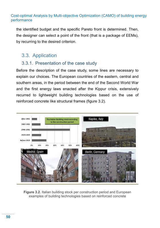
Cost-optimal Analysis by Multi-objective Optimization (CAMO) of building energy performance
50
the identified budget and the specific Pareto front is determined. Then,
the designer can select a point of the front (that is a package of EEMs),
by recurring to the desired criterion.
3.3. Application
3.3.1. Presentation of the case study
Before the description of the case study, some lines are necessary to
explain our choices. The European countries of the eastern, central and
southern areas, in the period between the end of the Second World War
and the first energy laws enacted after the Kippur crisis, extensively
recurred to lightweight building technologies based on the use of
reinforced concrete like structural frames (figure 3.2).
Figure 3.2. Italian building stock per construction period and European
examples of building technologies based on reinforced concrete

Cost-optimal Analysis by Multi-objective Optimization (CAMO) of building energy performance
51
These architectures are not equipped with thermal insulation, and this
concerns the large part of the present building stock, and thus these
buildings are characterized by quite high energy demands, above all for
the space heating in wintertime. With reference to the case study here
proposed, the considered building geometry (figure 3.3) is very similar to
those represented in figure 3.2. Indeed, the model has been designed in
order to be expressive of the aforementioned building stock.
Figure 3.3. The modeled residential building: a) prospectus b) axonometric c)
floor plan

Cost-optimal Analysis by Multi-objective Optimization (CAMO) of building energy performance
52
The building is supposed to be located in the Italian city of Naples. The
building is used for apartments and has an overall length, width and
height respectively equal to 24.8 m (north-south façade), 23.7 m (east-
west façade), 22.8 m (overall height). The entire architecture has six
floors, with four apartments at each one (i.e., 24 dwellings), each one of
110 m2. Two contiguous flats have a common balcony. As previously
said, the structural frame is made in reinforced concrete, with vertical
walls in hollow blocks (Uv = 1.4 W/m2K) and mixed ‘hollow brick-reinforced
concrete’ ceilings and roofs (Ur = 1.5 W/m2K). The windows have single
glasses, equipped with aluminium frames (Uw = 5.8 W/m2K).
All flats have been parted in an appropriate number of rooms, each one
equipped with a four-pipe fan-coil. The single apartment has two
exposures, being located at a building corner. The active system for the
microclimatic control supplies to the fan-coils:
hot water (45 °C, ΔT = -5 °C between supply and return pipes) in the
heating season,
chilled water (7 °C, ΔT = 5 °C) during the cooling season.
The heat and cold generations are guaranteed respectively by means of
a hot water boiler (low calorific value efficiency, η = 0.85) and an air-
cooled chiller (energy efficiency ratio, EER = 3.5). The inner height of the
single apartment is 3.3 m, the gross one is 3.8 m. All indoor spaces are
conditioned, and thus also the staircase. The global net conditioned area
is 3262 m2, the gross heated volume is 12396 m3.
EnergyPlus has been used for the creation of the model, firstly for the
definition of geometry and thermal zones, by means of the third-party
interface DesignBuilder [94], and then for the modeling of thermo-physical
properties of the building envelope, for the assignment of the schedules
of occupancy, lighting, set-point temperatures and, obviously, for the
entire modeling of the HVAC system.

Cost-optimal Analysis by Multi-objective Optimization (CAMO) of building energy performance
53
The building, in the starting configuration and thus before the energy
retrofit, is characterized by the following values of the objective functions
(note that the subscript BB means ‘base building’).
EPBB = 139 kWh/m2a DHBB = 34%
Then, the methodology previously presented has been applied and
described in the next lines of this chapter, in order to identify the cost-
optimal solution, in case of an energy-oriented refurbishment. After a
preliminary study of the existing building and of the possible ERMs, the
following measures of energy refurbishment have been taken into
account in the optimization study, because these are the ones that affect,
more than the others, the energy performance of the building:
Installation of a new external coating of the roof, by changing the
radiative characteristics, in order to reduce the heat gains.
Installation of external insulation of the roof, by means of installation
of rockwool panels.
Installation of external insulation of the vertical envelope, by means of
expanded polystyrene (EPS).
Installation of a mechanical ventilation system, for achieving a free
cooling when the temperature of the ambient air is lower compared to
the indoor. The system starts when, in the cooling season, there is a
minimum temperature difference between indoor air and ambient air,
equal to 2°C. Note that the adjective ‘free’ intends that the system is
not equipped with a chiller, and thus the energy consumption concerns
the mere fans.
Variation of the set points of indoor temperature, during both the
heating and cooling seasons.
Replacement of the single glazed windows with systems equipped
with low-emissive double glasses.

Cost-optimal Analysis by Multi-objective Optimization (CAMO) of building energy performance
54
Replacement of the present standard boiler with a condensing one (η
= 1.05).
Replacement of the air-cooled chiller with a water-cooled one (COP =
5.0), with the consequent installation of a well-sized cooling tower.
The design choices comply with the local construction standards.
Therefore, the following design variables (please, note that the number is
in the order of 10, as recommended by Wetter [95]) have been identified:
absorption coefficient of solar radiation of the roof (a). Note that the
thermal emissivity is commonly quite high for all construction
materials, with the exception of metallic ones;
thickness of the roof insulation (tr);
thickness of the insulation of vertical walls (tv);
free cooling by means the new mechanical ventilation system: yes/ no;
set point temperature of indoor air during the heating season (Theat);
set point temperature of indoor air during the cooling season (Tcool);
window: single/double glazed;
boiler: old standard / condensing one;
chiller: air- or water-cooled.
The values assumable by each variable and the investment costs (if
present) associated with these values are reported in table 3.2, where the
configuration of the base building is also shown. The values of the
investment costs have been obtained through quotations from suppliers
and according to the typical Italian market.
It is worthy to note that the number of energy simulations with EnergyPlus,
required for investigating all possible building configurations, would be
16384, while the optimization procedure takes a maximum of 750

Cost-optimal Analysis by Multi-objective Optimization (CAMO) of building energy performance
55
simulations, with a consequent saving of 95.5% of the computational
time.
In order to achieve the cost-optimal solution, since the maximum total
investment cost of the retrofit actions is 583573 €, the optimization study
has been performed for the following six budgets: 100000 €, 200000 €,
300000 €, 400000 €, 500000 €, 600000 € (nb = 6).
Table 3.2. Option values and investment cost (IC) of the design variables
DESIGN
VARIABLES OPTION VALUES
BASE
BUILDING IC [€]
a
0.05 31938 0.30 31938 0.70 ● - 0.95 31938
tr
0 cm ● - 3 cm 11023 6 cm 16886 9 cm 22750
tv
0 cm ● - 3 cm 152911 6 cm 174533 9 cm 196155
free cooling no ● - Yes 30112
Theat
19°C - 20 °C ● - 21 °C - 22 °C -
Tcool
24 °C - 25 °C - 26 °C ● - 27 °C -
window type
single glazed (Uw = 5.8 W/m2K)
● -
double glazed low-e (Uw = 1.9 W/m2K)
209711
boiler type old ● - condensing 32982
chiller type air-cooled ● - water-cooled 59925

Cost-optimal Analysis by Multi-objective Optimization (CAMO) of building energy performance
56
Please note that, as known, the energy efficiency of a building can be
achieved by means of: a) a proper design of the thermal envelope, b)
efficient systems and equipment for the microclimatic control (equipped
with suitable thermal generation devices for both heating and cooling) and
c) by means of a proper energy conversion in-situ by renewable energy
sources. For an existing building, the third strategy, and thus the
installation of renewable energy systems, is postponed to the
refurbishment of building envelope and of the heating/cooling system.
Indeed, the use of renewable would be a way for compensating, by
means of a clean energy conversion, the high energy demand of the
present building, without solving the waste of energy due to the poor
performance of the building itself. On the other hand, applied to
refurbished architectures, the clean energy conversion from renewables
could be used for other scopes, such as the indoor lighting or the
functioning of electrical devices. Therefore, in the present case study, the
attention has been focused on the renovation of the envelope and the
HVAC system, being these a priority also because of the effect on the
thermal comfort. In any case, a following optimization of the installable
renewables is recommended. The methodology here proposed can be
used also for this scope
3.3.2. Results and discussion
Figure 3.4 shows the Pareto fronts obtained for the six aforementioned
budgets. Here, the ‘best’ solution, with reference to each budget and
using the utopia point criterion, is highlighted by means of a bigger black
marker. The values assumed by the design variables in correspondence
of these best packages and the relative investment costs are listed in
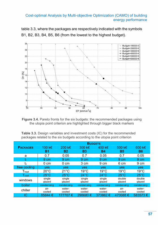
Cost-optimal Analysis by Multi-objective Optimization (CAMO) of building energy performance
57
table 3.3, where the packages are respectively indicated with the symbols
B1, B2, B3, B4, B5, B6 (from the lowest to the highest budget).
Figure 3.4. Pareto fronts for the six budgets: the recommended packages using
the utopia point criterion are highlighted through bigger black markers
Table 3.3. Design variables and investment costs (IC) for the recommended
packages related to the six budgets according to the utopia point criterion
BUDGETS PACKAGES 100 k€ 200 k€ 300 k€ 400 k€ 500 k€ 600 k€
B1 B2 B3 B4 B5 B6
a 0.7 0.05 0.7 0.05 0.7 0.05 tr 9 cm 9 cm 9 cm 9 cm 9 cm 9 cm tv 0 cm 0 cm 3 cm 9 cm 6 cm 9 cm
free cooling yes yes yes yes yes yes Theat 20°C 21°C 19°C 19°C 19°C 19°C Tcool 25°C 25°C 24°C 24°C 25°C 25°C
windows single glazed
single glazed
single glazed
single glazed
double glazed
double glazed
boiler condensing condensing condensing condensing condensing condensing
chiller air-
cooled water-cooled
water-cooled
water-cooled
air- cooled
water-cooled
IC 85844 € 177707 € 298680 € 373862 € 470088 € 583573 €

Cost-optimal Analysis by Multi-objective Optimization (CAMO) of building energy performance
58
It is well evident that all solutions (i.e., each point of the Pareto fronts)
determine a significant improvement compared to the base building
(EPBB=139 kWh/m2a, DHBB=34%). This underlines that the behavior of
the present building is unacceptable from both the point of views of
energy demand and thermal comfort.
Furthermore, figure 3.4 and table 3.3 show that the proposed optimization
procedure permits original and relevant remarks, by allowing the
definition of a ranking of the retrofit energy measures based on the
intervention priority. In other words, the ERMs that more influence the
objectives have a higher priority and a lower ranking.
As the budgets increase, the fronts obviously move left, and thus the
reliability of the optimization algorithm is confirmed. In detail, the most
significant shift occurs in the transition from 200000 € to 300000 €, which
corresponds to the introduction of the thermal insulation for the vertical
opaque walls. This measure highly influences both EP and DH.
The recommended solutions for the six budgets, summarized in table 3.3,
are deeply analyzed in the following lines. In correspondence of all these
solutions, three energy efficiency measures are always applied, and thus
the maximum insulation of the roof, the replacement of the boiler and the
introduction of the mechanical ventilation system. Therefore, these ERMs
have the lowest ranking, that means the highest priority. Hereafter, the
package of these three actions will be denoted with the adjective ‘basic’,
exactly because this is always present. In particular, B1 is characterized
by the application of the mere basic package, while in correspondence of
B2 also the water-cooled chiller and the low-a coating of the roof are
implemented. The low-a coating induces an increase of Theat, since the
mean radiant temperature of the roof decreases. The vertical insulation
is not yet introduced, although this action, as aforementioned, highly
affects both objectives, with an investment cost lower than 200000 €. This

Cost-optimal Analysis by Multi-objective Optimization (CAMO) of building energy performance
59
means that the basic package has the priority, and the application of this
annuls the economic possibility of applying also the wall thermal
insulation. Diversely, if the budget admits an investment of around
300000 € or more, the vertical insulation is always chosen, being
possible, according to the economic capacity, its adoption together with
the basic package. The vertical insulation produces a reduction of Theat
and an increment of Tcool, since this has an effect of increase of the mean
radiant temperature of the inner surfaces of the vertical opaque envelope.
In this way, the vertical insulation has a strong influence on the thermal
comfort, as shown in figure 3.5, where the trend of the recommended
solutions is depicted by means of a cubic polynomial fitting. It is evident
that, after the introduction of the vertical insulation (starting from B3), the
values of DH undergo small variations, and thus these tend to a horizontal
asymptote.
Figure 3.5. Trend of the recommended solutions according to the utopia point
criterion by means of cubic polynomial fitting

Cost-optimal Analysis by Multi-objective Optimization (CAMO) of building energy performance
60
Again, with reference to the recommended packages, the difference
between B3 and B4 is merely the adoption of the low-a coating of the roof
and the increased thickness of the vertical insulation, allowed because of
the increment in the money availability. The installation of new windows
with double and low-emissive glasses concerns only B5 and B6. Surely,
this induces lower thermal losses in winter and thus an increment of the
mean radiant temperature, by allowing a reduction of Theat. In summer,
contrasting effects happen. Indeed, the new glazed systems reduce the
entering solar radiation, even if also the thermal losses from the indoor
environment to the external one, in some hours (mainly in the
intermediate seasons), are lowered. Definitively, Tcool is improved (i.e.,
higher) compared to B3 and B4, even if it is at the same value of B1 and
B2. This retrofit measure has a lower priority compared to both the basic
package and vertical insulation, and, thus this is adopted only for high
economic availabilities. Moreover, B5 contemplates double glasses
without replacing the air-cooled chiller. Thus, the replacement of the
windows seems to have a higher priority compared to the adoption of a
new water-cooled chiller. The Pareto fronts for the budgets 400000 € and
500000 € are almost overlapped, and thus we could conclude that, under
these boundary conditions (e.g. kind of building, climate, etc.), the
replacements of chiller and windows have the same ranking with regards
to the considered objective functions, even if the first action is more
advantageous in a mere economic perspective.
Generally, under an economic point of view, the Pareto front at 500000 €
is worse than the one at 400000 €, and thus it could be excluded, ‘a priori’,
from the cost-optimal analysis. Moreover, it can be observed that, for B5,
the thickness of the vertical insulation is set to the value of 6 cm, even if
also the value of 9 cm is economically feasible. This could appear strange
but, actually, it is a relevant proof of the reliability of the methodology.

Cost-optimal Analysis by Multi-objective Optimization (CAMO) of building energy performance
61
Indeed, a higher thickness of the insulation would induce an increment of
EP, caused by a higher energy demand for the space cooling in summer,
because of the occurring of an indoor overheating phenomenon induced
by the hyper-insulation effect. About it, the air-cooled chiller does not
mitigate this negative impact. Finally, in this case, an increment of the
investment cost would determine a negative increment of the energy
demand. Diversely, for the other budgets, the maximum thickness of
vertical insulation is profitable. Indeed, the water-cooled chiller is adopted
and thus the energy demand during the cooling season has an effect on
the EP lower compared to the energy demand for the space heating.
Moreover, it is noted that the external coating of the roof, with a low-
absorption coefficient, is implemented only if part of the budget is still
available. It means that this energy efficiency measure has the lowest
priority. All told, the following ranking of the above-described retrofit
actions has been achieved:
1. basic package, and thus combination of external insulation of the roof,
replacement of the boiler with a condensing one and installation of a
mechanical ventilation system;
2. installation of external insulation of the vertical envelope;
3. replacement of the air-cooled chiller with a water-cooled chiller;
replacement of the single glazed windows with new system equipped
with double glasses, low-emissive;
4. installation of a new low-a coating (i.e., high-reflective) for the roof.
Finally, the designer should select the retrofit actions, depending on the
available budget, according to the shown priority.
After the optimization study above-reported in matter of energy
performance and thermal comfort, a further economic analysis is
necessary in order to detect the cost-optimal package and thus ‘the best

Cost-optimal Analysis by Multi-objective Optimization (CAMO) of building energy performance
62
budget’ that should be invested. Therefore, the global cost is calculated
for the solutions listed in table 3.3 and with reference to the base building,
in both cases of absence of incentives and in presence of a capital grant
(e.g., funding measures of the Governments according to policies of
sustainability), which covers the 50% of investment costs, as shown in
figure 3.6. The considered time is 30 years, as indicated in [7] for
residential applications.
Figure 3.6. Global costs of the recommended packages according to the utopia
point criterion in absence of incentives and in presence of a capital grant that covers 50% of investment costs
If incentives are not available, the cost-optimal packages are B1 and B3.
These allow an economic saving of about 330000 € compared to the base
building. In presence of an economic funding equal to 50% of the
investment costs, the best solution is clearly B3, with a saving of about
445000 €. As predicted, the solution B5 is worse than B4 under the point
of view of the cost-optimality.

Cost-optimal Analysis by Multi-objective Optimization (CAMO) of building energy performance
63
In the next study, the post-processing phase is performed by adopting the
comfort method for the multi-criteria decision-making. In particular, the
maximum acceptable value of percentage discomfort hours (DHmax) is set
at 10%. Really, depending on the required level of thermal comfort
(related to the building use), the methodology here proposed allows the
choice of the most proper level of comfort. Figure 3.7 and table 3.4 show
the recommended packages according to this different criterion of choice.
These are indicated with the symbols B1’, B2’, B3’, B4’, B5’, B6’. The
results are similar to those obtained by, using the utopia point method,
with some exceptions. First of all, it is noted that the budget 100000 €
does not provide acceptable solutions. This is a relevant result, showing
that a high level of thermal comfort requires a certain initial investment.
Figure 3.7. Pareto fronts for the six budgets: the recommended solutions using
the comfort criterion (DHmax= 10%) are highlighted through bigger black markers
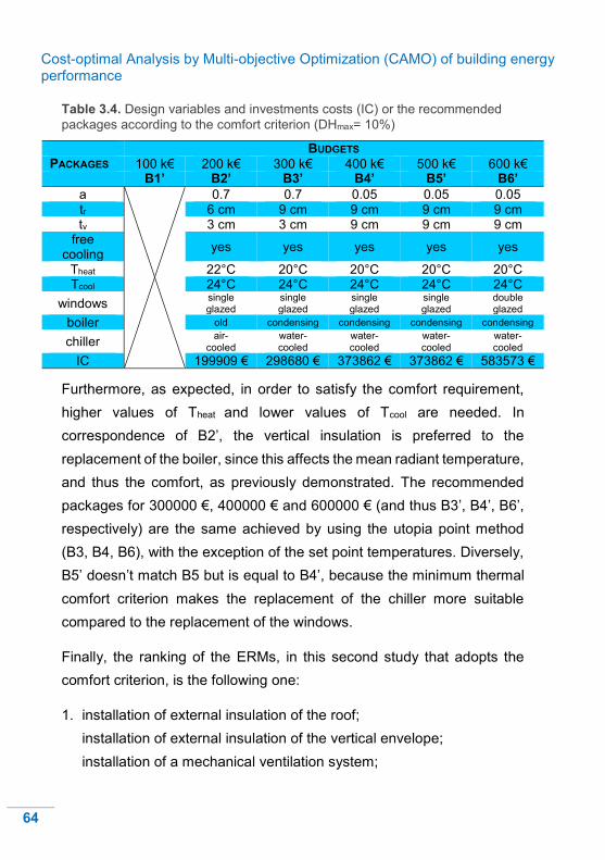
Cost-optimal Analysis by Multi-objective Optimization (CAMO) of building energy performance
64
Table 3.4. Design variables and investments costs (IC) or the recommended
packages according to the comfort criterion (DHmax= 10%)
BUDGETS PACKAGES 100 k€ 200 k€ 300 k€ 400 k€ 500 k€ 600 k€
B1’ B2’ B3’ B4’ B5’ B6’
a
0.7 0.7 0.05 0.05 0.05 tr 6 cm 9 cm 9 cm 9 cm 9 cm tv 3 cm 3 cm 9 cm 9 cm 9 cm
free cooling
yes yes yes yes yes
Theat 22°C 20°C 20°C 20°C 20°C Tcool 24°C 24°C 24°C 24°C 24°C
windows single glazed
single glazed
single glazed
single glazed
double glazed
boiler old condensing condensing condensing condensing
chiller air-
cooled water-cooled
water-cooled
water-cooled
water-cooled
IC 199909 € 298680 € 373862 € 373862 € 583573 €
Furthermore, as expected, in order to satisfy the comfort requirement,
higher values of Theat and lower values of Tcool are needed. In
correspondence of B2’, the vertical insulation is preferred to the
replacement of the boiler, since this affects the mean radiant temperature,
and thus the comfort, as previously demonstrated. The recommended
packages for 300000 €, 400000 € and 600000 € (and thus B3’, B4’, B6’,
respectively) are the same achieved by using the utopia point method
(B3, B4, B6), with the exception of the set point temperatures. Diversely,
B5’ doesn’t match B5 but is equal to B4’, because the minimum thermal
comfort criterion makes the replacement of the chiller more suitable
compared to the replacement of the windows.
Finally, the ranking of the ERMs, in this second study that adopts the
comfort criterion, is the following one:
1. installation of external insulation of the roof;
installation of external insulation of the vertical envelope;
installation of a mechanical ventilation system;

Cost-optimal Analysis by Multi-objective Optimization (CAMO) of building energy performance
65
2. replacement of the hot water boiler with a condensing one;
replacement of the air-cooled chiller with a water-cooled chiller;
3. replacement of the single glazed windows with new system equipped
with double glasses, low-emissive;
installation of a new low-a coating (i.e., high-reflective) for the roof.
Therefore, the utopia point criterion favors the replacement of the boiler
in order to obtain a greater reduction of EP, while, diversely, the comfort
criterion prefers the insulation of the envelope for achieving a relevant
reduction of DH.
Now, the global cost is calculated also for the solutions listed in table 3.4,
in both cases of absence of incentives and achievement of a capital grant
that covers 50% of the investment costs. The histograms are reported in
figure 3.8. The cost-optimal package, in both cases of absence and
presence of incentives, is B3’. This allows respectively an economic
saving of about 310000 € and 413000 € compared to the base building.
The designer can choose the utopia point or the comfort criterion for the
decision-making, depending on the need to assign the same importance
for EP and DH or, diversely, to obtain a certain level of thermal comfort.
However, in both cases, the proposed methodology allows the evaluation
of actual cost-optimal solutions, by ensuring, at the same time, that a
thermal comfort criterion is satisfied. This is one of the original aspects of
this study. Indeed, standard approaches for the cost-optimal analysis
contemplate the thermal comfort only in a generic way. Moreover, these
assume that the packages of energy measures are chosen empirically,
by trial, and thus the entire domain of possible solutions is not
exhaustively investigated. Consequently, a reliable cost-optimality is not
guaranteed.

Cost-optimal Analysis by Multi-objective Optimization (CAMO) of building energy performance
66
Figure 3.8. Global costs of the recommended packages according to the
comfort criterion (DHmax= 10%) in absence of incentives and in presence of a capital grant that covers 50% of investment costs
Again with reference to the proposed case study, it can be observed that
both methods for the multi-criteria decision-making provide the same
cost-optimal package, with the exception of the set point temperature
during the space heating. This cost-optimal package corresponds to the
budget of 300000 €, which can be thus defined as the ‘cost-optimal
budget’. This is a very relevant result, which shows that, in this case, the
methods provide equivalent information about the individuation of the
best solutions for the following cost-optimal analysis. Moreover, it should
be noted that the cost-optimal budget is the one that, by increasing the
money availability of the same amount (increment of 100000 €), produces
the highest left shift of the Pareto front compared to the previous one (see
figures 3.4 and 3.7). This is justified by the strong correlation between the
reduction of EP and the cost-optimality.
Two different points (namely B3 and B3’) of the Pareto front of the budget
300000 € identify the cost-optimal solutions, obtained by means of the

Cost-optimal Analysis by Multi-objective Optimization (CAMO) of building energy performance
67
application of the two methods. After the evaluation of the cost-optimal
budget and the relative Pareto front, the designer can analyze the
different solutions on the front and then he can choose according to his
own needs and purposes. About it, eight solutions, identified with the
numbers from 1 to 8, are available, as shown in figure 3.9 and table 3.5.
Figure 3.9. Pareto front in correspondence of the cost-optimal budget (300 k€)
Table 3.5. Design variables and investments costs for the points on the Pareto
front relative to the cost-optimal budget (300000 €)
POINTS ON THE PARETO FRONT RELATIVE TO THE BUDGET OF 300000 €
1 2 3 4 5 6 7 8
a 0.7 0.7 0.7 0.7 0.7 0.7 0.05 0.05 tr 9 cm 9 cm 9 cm 9 cm 9 cm 9 cm 9 cm 9 cm tv 3 cm 3 cm 3 cm 3 cm 3 cm 3 cm 6 cm 6 cm
free cooling
yes yes yes yes yes yes yes yes
Theat 19°C 19°C 20°C 19°C 19°C 20°C 21°C 22°C Tcool 27°C 26°C 26°C 25°C 24°C 24°C 24°C 24°C
windows single glazed
single glazed
single glazed
single glazed
single glazed
single glazed
single glazed
single glazed
boiler condensing condensing condensing condensing condensing condensing condensing condensing
chiller water- cooled
water- cooled
water- cooled
water- cooled
water- cooled
water- cooled
air-cooled air-cooled
IC 298680 € 298680 € 298680 € 298680 € 298680 € 298680 € 292315 € 292315 €

Cost-optimal Analysis by Multi-objective Optimization (CAMO) of building energy performance
68
It should be noted that these packages are very similar, with the exception
of the values of set point temperatures, which influence consistently the
objectives. Moreover, the solutions with lower values of EP (i.e., 1, 2, 3)
are characterized by the water-cooled chiller and 3 cm of vertical
insulation, while those with lower values of DH (i.e., 7 and 8) have the air-
cooled chiller and 6 cm of vertical insulation. Thus, the EEM that mainly
affects the EP is the replacement of the HVAC generation systems, while
the one that has a more significant impact on the DH is the vertical
insulation. However, the recommended packages are those that ensure
a good trade-off between the objectives, and thus the solutions 4, 5 (the
‘best’ according to the utopia point criterion, B3) and 6 (considering the
comfort criterion, B3’). These give the same retrofit actions, by differing
only in the set point temperatures. Finally, the cost-optimal set of actions
is identified, and the designer has only to select one of these three points
(i.e., the values of Theat and Tcool), according to the desired level of thermal
comfort.
In conclusion, the cost-optimal solution is characterized by the following
ERMs:
installation of external insulation of the roof, with a thickness of 9 cm;
installation of external insulation of the vertical envelope, with a
thickness of 3 cm;
implementation of a mechanical ventilation system, for the space free
cooling (when available depending on the temperature difference
between ambient and indoor airs);
Theat = 19 / 20 °C, depending on the required comfort level in winter;
Tcool = 24 / 25°C, depending on the required comfort level in summer;
replacement of the old boiler with a condensing one;
replacement of the air-cooled chiller with a water-cooled chiller.

Cost-optimal Analysis by Multi-objective Optimization (CAMO) of building energy performance
69
The achieved economic saving varies between the aforementioned
values, depending on the chosen set point temperatures and the absence
or achievement of economic incentives for the energy refurbishment of
buildings. Finally, it should be noted that the CAMO can be easily
extended to more complex buildings and new constructions, allowing
original conclusions and in-depth investigations concerning all the
available EEMs, in order to evaluate the cost-optimal package of the
energy actions for both existing and new buildings, by taking into account
also thermal comfort.
Final remarks
All told, the computational burden and complexity required by CAMO
impedes the application of this powerful methodology to each single
building. This represents the main weakness of CAMO. Therefore, the
purpose of achieving global indications about the cost-optimal mix of
ERMs fora group of buildings has led to the development of SLABE, as
discussed in the next chapter.

Simulation-based Large-scale uncertainty/ sensitivity Analysis of Building Energy performance (SLABE)
70
How to achieve global indications about the cost-optimality
of energy retrofitting the existing building stock?
CHAPTER 4. Simulation-based Large-scale uncertainty/ sensitivity Analysis of Building Energy performance (SLABE)
4.1. Introduction
Since the cost-optimal analysis can’t be performed to each building, for
reason of complexity, reference buildings (RefBs) have to be defined to
represent the national building stock. They should cover all the building
categories, where a category is meant as a stock of buildings, which
share climatic conditions (location), functionality, construction type.
Therefore, the cost-optimal analysis should be applied to these RefBs, in
order to detect cost-optimal packages of energy measures [32, 66]. Then,
the results achieved for a RefB should be extended to the other buildings
of the represented category [96]. However, does this procedure ensure
reliable results for all the buildings of the category? Otherwise, how to
investigate, in a more rigorous way, energy performance and cost-
optimality of a building category?
The energy analysis of a building stock, rather than of single buildings, is
essential when the purpose is to quantify the global potential of energy
savings [97] or to give general indications about cost-optimal packages
of energy measures. The scientific literature shows different methods for
assessing the energy performance of a building stock. However, most of
these studies just provide a picture of the existing stock starting from data
collections [97-101], and/or explore the potential saving induced by few

Simulation-based Large-scale uncertainty/ sensitivity Analysis of Building Energy performance (SLABE)
71
energy measures in a simplified manner, without considering the cost-
optimal analysis [97, 99].
This chapter attempts to solve the mentioned issues by proposing a novel
multi-stage methodology, which provides a robust analysis of energy
performance and cost-optimal retrofit solutions for a building category.
The methodology is denoted as ‘Simulation-based Large-scale
uncertainty/sensitivity Analysis of Building Energy performance’
(SLABE). Indeed, it is based on uncertainty analysis (UA) and sensitivity
analysis (SA) of building performance, which are performed by means of
the coupling between EnergyPlus and MATLAB. SLABE investigates the
influence of well-selected retrofit actions on energy consumption and
global cost related to a sampling set of buildings representative of a
category. The main goals are:
GOAL I. to detect the package of actions that represents the cost-optimal
solution for most buildings of the category.
GOAL II. to evaluate the effectiveness of current policy of state incentives
directed to such actions and to propose possible improvements
for achieving the best ratio between energy savings and state
disbursement.
In the following lines, the methodology is first described and then applied
to a specific category: office buildings built in South Italy in the period
1920-1970.
Alike CAMO, SLABE can be adopted either as a stand-alone
methodology for the investigation of a building category or as a part (stage
I) of the macro-methodology (CASA) proposed in this thesis (chapter 6).

Simulation-based Large-scale uncertainty/ sensitivity Analysis of Building Energy performance (SLABE)
72
4.2. Methodology
This study proposes a novel methodology for providing a robust cost-
optimal analysis of energy retrofitting solutions for a building stock. The
cost-optimality is estimated in line with EPBD Recast, but the developed
approach introduces an original aspect that regards the simultaneous
investigation of different buildings belonging to the same category. The
methodology presents a multi-stage framework, which allows to assess
the influence of some energy retrofit measures on primary energy
consumption (PEC) and global cost (GC) related to a representative
sample of buildings; this should be large enough to represent the
considered category significantly. The outcomes are investigated and
collected by means of UA and SA, which provide general conclusions for
the whole stock. In particular, such analysis allows to detect the retrofit
actions that have the strongest effect on PEC and GC savings, in order
to reach the two ultimate aims mentioned in the introduction.
It is emphasized that UA and SA are generally carried out for a single
building [83, 88, 102, 103], in order to assess how the variations of some
uncertain parameters affect energy performance. On the contrary, this
study performs UA and SA on a large scale, since the uncertainty in the
parameters is generated by the investigation of several buildings
belonging to the same category. Thus, the developed methodology is
denoted as Simulation-based Large-scale Uncertainty/Sensitivity
Analysis of Building Energy performance (SLABE).
SLABE is based on the coupling between EnergyPlus and MATLAB.
EnergyPlus is chosen as BPS (building performance simulation) tool
because: it’s a whole building energy simulation program that allows a
detailed evaluation of each term of PEC; it works with text-based format
inputs (.idf) and outputs (.csv), which facilitate the interaction with
mathematical tools. MATLAB is chosen for UA, SA and post-processing

Simulation-based Large-scale uncertainty/ sensitivity Analysis of Building Energy performance (SLABE)
73
because: it has a very strong capability; it can automatically launch
EnergyPlus as well as manipulate EnergyPlus input and output files.
The UA is performed by means of Monte Carlo analysis (MCA), which is
widely applied to BPS [83, 88, 102–104]. As aforementioned, the UA is
carried out on a large scale in order to investigate the distributions of
some performance indicators within a sample of buildings, representative
of a certain category. Thus, the ranges of uncertainty of the parameters
are wider than when the UA is applied to a single building [83, 88, 102,
103]. As regards the SA, a global approach is used through the
assessment of the standardized rank regression coefficients (SRRCs). In
building energy analysis, the global approach is more reliable than the
local one [73, 87] and regression methods are the most used [87].
Moreover, BPS tools generally generate nonlinear, multi-modal,
discontinuous outputs [105, 106]. Thus, the SRRCs are selected as
sensitivity indices, since they are fine for non-linear (but monotonic)
functions between inputs and outputs. This choice is largely shared in the
BPS community [107, 108]. In particular, the SRRC provides a measure
of how influential a parameter is on an output, based on the effect of
moving such parameter away from its expected value while retaining all
other parameters constant. It can vary from –1 to 1; a positive value
indicates that the parameter and the output change with the same sign,
while the opposite occurs for a negative value.
SLABE consists of two main stages, which are subdivided respectively in
two and three steps, as shown in figure 4.1 and described in the following
subsections.

Simulation-based Large-scale uncertainty/ sensitivity Analysis of Building Energy performance (SLABE)
74
Figure 4.1. Framework of the developed methodology (SLABE). The symbol e+
indicates the data provided by EnergyPlus and handled by MATLAB, required for the evaluation of PEC (and so GC)

Simulation-based Large-scale uncertainty/ sensitivity Analysis of Building Energy performance (SLABE)
75
4.2.1. Stage I. Assessment of energy demand and thermal comfort (discomfort hours)
Energy demand and thermal comfort are investigated, by means of UA
and SA. In particular four performance indicators (PIs) are considered:
annual energy demand for heating, EDh [kWh/m2a];
annual energy demand for cooling, EDc [kWh/m2a];
percentage of discomfort hours on occupied hours, during the heating
season, DHh [%];
percentage of discomfort hours on occupied hours, during the cooling
season, DHc [%].
The energy demand is the annual request of energy for micro-climatic
control per unit of conditioned area.
As regards the assessment of the discomfort hours (DH), the weighted
under- or over-heating [88]/ cooling hours criterion, which is described in
section 3.2.1, is used.
The four PIs are first investigated for the existing building stock (step 1)
and then for the renovated building stock (step 2), namely in presence of
energy efficiency measures for the reduction of energy demand (EEMsd).
In the second case, also the annual values of energy demand (ED) and
discomfort hours (DH) are considered in order to explore the overall
effects of the EEMsd.
Step 1. Analysis of the existing building stock
The existing building stock is characterized by detecting n key parameters
relevant to energy demand and thermal comfort. A range of variability and
a probability distribution (e.g., uniform or normal) are assigned to each
parameter in order to represent the whole building category. A reference
building (RefB) related to the investigated category can be exploited to
set the mean values of such distributions, as shown in section 4.3.1. The
Simulation-based Large-scale uncertainty/ sensitivity Analysis of Building Energy performance (SLABE)
76
selected parameters are classified in three groups, respectively related to
geometry (form and orientation), envelope (thermo-physical
characteristics of materials) and other parameters that can’t be placed in
the first two groups (e.g., set point temperatures, internal loads, people
density). SLABE is limited to rectangular buildings. This choice facilitates
the parameterization process [104], and it’s proper for most building
categories because of the high percentage of rectangular shapes.
The three groups of parameters and their correlated ranges define the
sample space to investigate. Latin hypercube sampling (LHS) is applied
to these parameters within a Monte Carlo framework, in order to generate
N samples, which correspond to N building model instances and, thus, to
N EnergyPlus simulations. These samples constitute S1, representing the
existing building stock. LHS is used because it ensures uniformity and
coverage in the sample space, thanks to its efficient stratification
properties [109, 110]. Indeed, it’s widespread in the scientific literature
concerning BPS [88, 102, 108, 111, 112]. It is noted that the value of N
must be chosen carefully, in order to thoroughly represent the building
stock, as argued in section 4.3.2.
The N building model instances are then run in EnergyPlus, by means of
the coupling with MATLAB, obtaining N sets of values of the four PIs.
Thus, the UA and the SA (assessment of the SRRCs) are performed
respectively to explore the distributions of such indicators and to detect
which parameters have the most/least influence.
Step 2. Analysis of the renovated building stock
After studying the existing building stock, an analogous analysis is
performed on the renovated building stock. In particular, some EEMsd are
introduced. Each EEMd is parameterized through a boolean parameter,
which assumes the value of 0 if the relative measure is absent, 1 if

Simulation-based Large-scale uncertainty/ sensitivity Analysis of Building Energy performance (SLABE)
77
present. These new parameters vary according an uniform distribution,
so that the probability that one EEMd occurs is equal to the 50%.
Furthermore, the implementation of the EEMsd generally requires the
introduction of other parameters (e.g., the thermo-physical characteristics
of thermal insulation), for a total of new e parameters.
Therefore, the renovated building stock is defined by (n + e) parameters
– n for the existing buildings and e for the EEMsd – whose sampling leads
to the second set S2, consisting of N samples alike S1. In particular, a
correspondence between S1 and S2 is established, as shown in table 4.1.
Each element of S2 provides the same values of the first n parameters
assumed by the homologous element of S1, while the remaining e
parameters are sampled by LHS. In light of this, S2 gathers the same
building instances of S1, but in presence of one or more EEMsd. This
expedient allows the direct comparison between the two sets (sample by
sample), by detecting the effects of some EEMsd on each building
instance.
Table 4.1. Framework of the sampling set S2, which represents the renovated
building stock
SAMPLING
SET
S2
PARAMETERS DESCRIBING THE
EXISTING BUILDING STOCK
PARAMETERS DESCRIBING THE
ENERGY EFFICIENCY MEASURES
p1 p2 … pn-1 pn pn+1 pn+2 … pn+e-1 pn+e
SA
MP
LE
S
1
2
…
N - 1
N
The N building model instances, gathered in S2, are run in EnergyPlus in
order to evaluate the new sets of values assumed by the four PIs. At this
LHS set S1

Simulation-based Large-scale uncertainty/ sensitivity Analysis of Building Energy performance (SLABE)
78
point, the UA allows the estimation of the effects induced by the EEMsd
on energy demand and thermal comfort in the heating and cooling
seasons. In addition, the values of the SRRCs are assessed for the
boolean parameters representing the EEMsd, in correspondence of EDh,
EDc, DHh, DHc, ED, DH. Thus, the SA allows to detect the most influential
EEMsd on the seasonal and annual values of energy demand and
discomfort hours.
4.2.2. Stage II. Assessment of primary energy consumption and global cost
The potential savings in PEC and GC induced by well-selected energy
retrofit measures are investigated. Since the sampling sets reliably
represent the building stock, the outcomes are valid for the whole
category. It is recalled that the methodology deals with two perspectives,
respectively related to collectives interests (PEC savings) and private
interests (GC savings). On one hand, it aims to evaluate the effectiveness
of the policy of state incentives for ERMs and to provide possible
improvements. On the other hand, it points to detect a package of ERMs,
which represents the cost-optimal solution for most buildings of the
analyzed category.
The PEC is an appropriate metric according to EPBD Recast. It
represents the sum of the different components of the building energy
use, which are converted by means of primary energy factors. Heating,
cooling, ventilation, pumps and fans, domestic hot water (DHW), lighting,
electrical equipment are considered. If RESs are present, produced and
used energy must be subtracted to the previous terms, in a consistent
way. SLABE calculates the PEC through the post-process performed in
MATLAB, after EnergyPlus simulations. This expedient allows the
reduction of the computational time [72]. More in detail, EnergyPlus

Simulation-based Large-scale uncertainty/ sensitivity Analysis of Building Energy performance (SLABE)
79
provides the hourly values of the energy demand for heating, cooling,
DHW and electricity (which gathers the remaining components of building
energy use). These values are handled in MATLAB. First, heating,
cooling and DHW demands are turned into hourly demand of electricity
or fuel (depending on the type of HVAC system) through the hourly
performance curves of the HVAC system. Then, the overall values of
electricity and fuel demand are converted in primary energy, by means of
primary energy factors. The PEC is so calculated. In presence of RESs,
EnergyPlus also yields the hourly values of produced energy. If produced
energy is consumed according to a hourly balance, it represents a
subtractive term in PEC evaluation.
The GC over the lifecycle of the buildings is calculated in MATLAB,
according to the guidelines of EPBD Recast. The real interest rate and
the energy price escalation rate are respectively set equal to 3% and 2%.
The annual energy demand is assumed constant during the calculation
period.
The exploration of the achievable savings in PEC and GC is carried out
in three steps, in order to consider the effects produced by three distinct
groups of energy retrofit measures: replacement of the primary
heating/cooling system (step 3), installation of RESs (step 4),
implementation of EEMsd (step 5).
Step 3. Replacement of the primary heating/cooling system
The replacement of the primary heating/cooling (HVAC) system is initially
considered as the only possible measure, in order to detect the impact of
new efficient systems on PEC and GC. In fact, this generally represents
the most influential retrofit action on energy and economic savings [72].
The PEC-GC analysis is performed (see figure 4.1). Specifically, the
values of PEC and GC are calculated for each sample of S1 (existing

Simulation-based Large-scale uncertainty/ sensitivity Analysis of Building Energy performance (SLABE)
80
building stock) in correspondence of the reference HVAC system and of
different new efficient options. The potential savings are then evaluated.
Hence, the best configurations of the HVAC system are identified, as
regards respectively energy and cost perspectives. In the first case, the
best solution is the one that ensures the highest PEC saving in the
building stock. In the second case, it is the one that leads to the highest
number of buildings (samples) with positive GC savings; this represents
the cost-optimal configuration. The best compromise between these two
perspectives is investigated, by means of the concurrent representation
of PEC and GC savings:
mean values are considered for PEC savings, because they are
proportional to the energy saving in the whole stock;
the box plot is chosen for the representation of GC savings, because
it allows to estimate, qualitatively, the percentage of buildings
characterized by cost savings.
The described analysis is carried out in absence and in presence of state
incentives in order to examine the effect of the current policy of grants
addressed to energy retrofit actions. The cost-optimal solution refers to
the presence of current incentives.
Eventually, a new incentive strategy is devised to obtain a better
congruence between the two investigated perspectives (PEC and GC
savings). The aim is to harmonize them, in such a way that the best
solution for the single building corresponds to the best solution for the
collectivity. The best configurations of the HVAC system are identified
also in this in case.
In order to compare the two strategies of current and proposed incentives,
some reasonable hypothesis are assumed. First, only the HVAC system
which ensures the highest values of GC savings for the whole category
can be implemented. Secondly, each building implements such HVAC

Simulation-based Large-scale uncertainty/ sensitivity Analysis of Building Energy performance (SLABE)
81
system only if the latter provides an economic benefit (positive value of
GC saving); otherwise it keeps its reference system. In particuar, the
percentage of samples with positive GC savings is denoted with p. In
these assumptions, the actual values of PEC savings and of state
disbursement for incentives can be calculated by multiplying by p the
values obtained for the whole sampling set. In order to point out the
advantages induced by proposed incentives, the two incentive strategies
are analyzed through the following indicators:
actual value of the average saving in primary energy consumption per
building, dPECb [kWh/a];
actual value of the average state disbursement per building, Db [€];
ratio between dPECb and Db, π [kWh/€ a]; it’s a sort of state profit,
representing the potential energy saving in correspodence of an
unitary disbursement.
Therefore, this step allows to:
detect the cost-optimal HVAC system, when the replacement of such
system is the unique implemented EEM;
evaluate the effectiveness of current incentives directed to HVAC
systems and to provide a more efficacious strategy.
Step 4. Installation of RESs
The potential savings in PEC and GC induced by the installation of RESs
are investigated for S1.
First, the PEC-GC analysis is performed in presence of the reference
HVAC system, in order to assess how the mere implementation of a RES
influence PEC and GC. The best configurations of the RES (e.g., area of
PV panels), as for PEC and GC savings, are detected in absence and in
presence of current state incentives Furthermore, A new incentive

Simulation-based Large-scale uncertainty/ sensitivity Analysis of Building Energy performance (SLABE)
82
strategy is conceived for the considered RES, and the best configurations
are detected also in this case. This procedure allows to:
determine the cost-optimal configuration of the RES;
evaluate the effectiveness of incentives directed to the considered
RES and to provide a more efficacious strategy.
If more RESs are examined, the same procedure is repeated for each of
them.
Then, well-selected combinations of HVAC system and RESs are
investigated by assessing PEC and GC savings in presence of current
incentives. These combinations are identified on the basis of:
previous results achieved in correspondence of the mere
implementation respectively of new HVAC systems (step 3) and RESs
(first part of step 4);
pecularieties of the explored building category in terms of energy
performance.
Eventually, this step identifies:
the cost-optimal combination between the replacement of the HVAC
system and the installation of RESs, when merely these energy
measures are implemented.
Step 5. Implementation of EEMsd
The effects of EEMsd on PEC and GC are explored. In this regard, the
SA performed in stage I (step 2) identifies the EEMsd which have a
significant influence on the annual value of energy demand. This step
considers only these EEMsd, since the remaining ones are not convenient
from both analyzed perspectives. Thus, a new set S3 is generated through
exhaustive sampling, in order to represent all the np possible packages
(combinations) of the contemplated EEMsd. S3 has a framework similar
to S2. More in detail, it collects np·N’ samples, which are composed of np

Simulation-based Large-scale uncertainty/ sensitivity Analysis of Building Energy performance (SLABE)
83
groups of N’ samples. N’ denotes the minimum number of samples
required to significantly describe the building stock. It can be identified
only after the UA performed in stage I (step 1); that’s why it generally
doesn’t coincide with N. Each of the np groups of S3 gathers the same
buildings, represented by the first N’ samples of the set S1, in presence
of one of the np possible EEMsd packages, so that all packages are
covered.
Hence, the potential savings in PEC and GC induced by the EEMsd are
investigated, by referring to S3. The analysis follows the logical order used
in step 4.
First, the reference HVAC system is considered. The best packages of
EEMsd, as for PEC and GC savings, are detected in absence and in
presence of state current incentives. Furthermore, new incentives are
devised for the considered EEMsd and the best packages are found out
also in this case. This procedure allows to:
identify the cost-optimal package of EEMsd, when only these energy
measures are applied;
evaluate the effectiveness of incentives directed to the considered
EEMsd and to provide a more efficacious strategy.
Then, PEC and GC savings are evaluated in correspondence of well-
selected combinations of HVAC system, RESs and EEMsd, in order to
find the cost-optimal package of retrofit actions. Likewise step 4, the
examined combinations are chosen on the basis of previous results and
energetic characteristics of the building category. Eventually, this step
identifies:
the cost-optimal package of ERMs, including replacement of the
HVAC system, installation of RESs and implementation of EEMsd; if
different packages ensure similar values of GC savings, the thermal

Simulation-based Large-scale uncertainty/ sensitivity Analysis of Building Energy performance (SLABE)
84
comfort can be used as discriminating criterion, on the basis of the
results achieved in stage I (step 2).
4.3. Application
4.3.1. Presentation of the case study
The methodology is applied to a building category with a large amount of
available data. In detail, Office buildings built in South Italy in the period
1920-1970 are investigated. A research study performed by ENEA [113]
(Italian national agency for new technologies, energy and sustainable
economic development) provides a deep statistical analysis of structural
characteristics and plant conditions of the Italian office building stock.
This study defines two RefBs respectively for office buildings built in the
period 1920-1970 and from 1971 until now. Buildings built in the period
1920-1970 are considered in this study, because they are characterized
by worse energetic performance compared to more recent ones. Thus,
the energetic retrofit of these buildings can induce high energy savings.
Moreover, they represent a significant percentage (32.4%) of the national
office building stock.
South Italy is chosen as geographical location for two main reasons. First,
the scientific literature concerning the study of office buildings in South
Italy is quite meager. Secondly, a high percentage (around 60%) of such
building dates back before 1970 [113]. Thus, investigated buildings cover
a wide segment of office buildings in South Italy and ensure high energy
saving potentials, as aforementioned.
The IWEC weather data file [86] of the city of Naples is used in
EnergyPlus simulations, because it is the second district in South Italy
regarding the number of office buildings. The first district is Lecce, but
Naples is preferred because of its climatic conditions, which are close to

Simulation-based Large-scale uncertainty/ sensitivity Analysis of Building Energy performance (SLABE)
85
average conditions in South Italy. Therefore, the results obtained for
Naples can be extended to many other cities of South Italy with an
acceptable approximation.
Reference building (RefB)
The considered RefB has a rectangular shape, thus perfectly fits to the
developed methodology. The structural frame is in reinforced concrete;
the vertical walls are made of two layers of bricks separated by an air gap;
a structure in mixed brick-reinforced concrete characterizes floor and
roof. Table 4.2 shows information about the stratigraphy of these
elements. The composition of internal walls and ceilings are not indicated
by ENEA; thus, they are supposed to be made of 0.15 m of concrete. The
windows are made of singles glasses and wooden frames (Uw=5.0
W/m2K). Their height is equal to 1.5 m. There is no solar shading.
All the other characteristics related to geometry, envelope and operation
are reported in table 4.3, in the column denoted with RefB; the other
columns are explained in the next subsection.
The defintion of the HVAC system is not explicit, since only statistical data
are reported by ENEA. Thus, this study is based on the following
assumptions. Fan coils and hot water radiators are alternately considered
as heating terminals; indeed the presence of one or the other can
significantly affect energy performance and thermal comfort. Cooling
terminals always consist of fan coils, which allow to investigate different
options of the primary cooling system. The primary heating system is a
natural gas boiler, with nominal efficiency (η, related to the low calorific
value) equal to 0.85, indicated with reference boiler (RB). The primary
cooling system is an air-cooled chiller, with nominal energy efficiency ratio
(EER) equal to 2.2, indicated with reference chiller (RC). There aren’t
RESs.

Simulation-based Large-scale uncertainty/ sensitivity Analysis of Building Energy performance (SLABE)
86
Table 4.2. Reference building: stratigraphy of floor, external walls and roof. The
values of solar absorptance (a) are indicated only for the external layers
t
[m] k
[W/m K] d
[kg/m3] c
[J/kg K] RT *
[m2 K/ W] a
FLOOR
Cobblestone 0.18 0.70 1500 880 - -
Floor Block 0.18 0.66 1800 840 - -
Clay 0.06 0.12 450 1200 - -
Screed 0.03 0.90 1800 840 - -
Tiles 0.02 1.00 2300 - -
EXTERNAL WALLS
External Brick 0.12 0.72 1800 840 - 0.5
Air Gap 0.20 - 1.03 1010 0.156 -
Internal Brick 0.08 0.90 2000 840 - -
Plaster 0.02 1.4 2000 820 - -
ROOF
Cement 0.03 1.40 1000 - 0.5
Screed 0.03 1.40 400 1000 - -
Expanded Clay 0.05 0.27 900 1000 - -
Roof Block 0.22 0.66 1800 840 - -
Plaster 0.02 0.70 800 1000 - -
*RT is the thermal resistance

Simulation-based Large-scale uncertainty/ sensitivity Analysis of Building Energy performance (SLABE)
87
Table 4.3. Parameters describing the building stock: value in the RefB; distribution in the
stock; mean value (μ) and standard deviation (σ) for normal distributions; range of variability
PARAMETERS RefB DISTRIBUTION μ σ RANGE
GE
OM
ET
RY
p1 Orientation (North Axis) 0° uniform - - 0; ±30; ±60; 90
p2 Area of each Floor [m2] 216 uniform - - 100 ÷ 500
p3 Form Ratio 1.5 uniform - - 1 ÷ 5
p4 Floor Height [m] 3.4 uniform - - 2.7 ÷ 4.2
p5 Window to Wall Ratio: S 29% uniform - - 10 ÷ 40
p6 Window to Wall Ratio: E 33% uniform - - 10 ÷ 40
p7 Window to Wall Ratio: N 17% uniform - - 10 ÷ 40
p8 Window to Wall Ratio: W 33% uniform - - 10 ÷ 40
p9 Number of Floors 2 uniform 1; 2; 3; 4; 5
EN
VE
LO
PE
p10 Air Gap RT [m2 K/W] 0.156 normal RefB 0.01 0.116 ÷0.196
p11 Roof a 0.5 normal RefB 0.2 0.1 ÷ 0.9
p12 External Walls a 0.5 normal RefB 0.2 0.1 ÷ 0.9
p13 Thickness of Concrete [m] 0.15 normal RefB 0.05 0.05 ÷ 0.25
p14 Type of Glass Single uniform - - Single/Double
p15 Type of Frame Wood uniform - - Wood/Aluminum
p16 Clay t [m] 0.06 normal RefB 0.2 μ (μ – 3σ) ÷ (μ + 3σ)
p17 Clay k [W/m K] 0.12 normal RefB 0.2 μ (μ – 3σ) ÷ (μ + 3σ)
p18 Clay d [kg/m3] 450 normal RefB 0.2 μ (μ – 3σ) ÷ (μ + 3σ)
p19 Clay c [J/kg K] 1200 normal RefB 0.2 μ (μ – 3σ) ÷ (μ + 3σ)
p20 Expanded Clay t [m] 0.05 normal RefB 0.2 μ (μ – 3σ) ÷ (μ + 3σ)
p21 Expanded Clay k [W/m K] 0.27 normal RefB 0.2 μ (μ – 3σ) ÷ (μ + 3σ)
p22 Expanded Clay d [kg/m3] 900 normal RefB 0.2 μ (μ – 3σ) ÷ (μ + 3σ)
p23 Expanded Clay c [J/kg K] 1000 normal RefB 0.2 μ (μ – 3σ) ÷ (μ + 3σ)
p24 External Brick t [m] 0.12 normal RefB 0.2 μ (μ – 3σ) ÷ (μ + 3σ)
p25 External Brick k [W/m K] 0.72 normal RefB 0.2 μ (μ – 3σ) ÷ (μ + 3σ)
p26 External Brick d [kg/m3] 1800 normal RefB 0.2 μ (μ – 3σ) ÷ (μ + 3σ)
p27 External Brick c [J/kg K] 840 normal RefB 0.2 μ (μ – 3σ) ÷ (μ + 3σ)
p28 Floor Block t [m] 0.18 normal RefB 0.2 μ (μ – 3σ) ÷ (μ + 3σ)
p29 Floor Block k [W/m K] 0.66 normal RefB 0.2 μ (μ – 3σ) ÷ (μ + 3σ)
p30 Floor Block d [kg/m3] 1800 normal RefB 0.2 μ (μ – 3σ) ÷ (μ + 3σ)
p31 Floor Block c [J/kg K] 840 normal RefB 0.2 μ (μ – 3σ) ÷ (μ + 3σ)
p32 Internal Brick t [m] 0.08 normal RefB 0.2 μ (μ – 3σ) ÷ (μ + 3σ)
p33 Internal Brick k [W/m K] 0.9 normal RefB 0.2 μ (μ – 3σ) ÷ (μ + 3σ)
p34 Internal Brick d [kg/m3] 2000 normal RefB 0.2 μ (μ – 3σ) ÷ (μ + 3σ)
p35 Internal Brick c [J/kg K] 840 normal RefB 0.2 μ (μ – 3σ) ÷ (μ + 3σ)
p36 Roof Block t [m] 0.22 normal RefB 0.2 μ (μ – 3σ) ÷ (μ + 3σ)
p37 Roof Block k [W/m K] 0.66 normal RefB 0.2 μ (μ – 3σ) ÷ (μ + 3σ)
p38 Roof Block d [kg/m3] 1800 normal RefB 0.2 μ (μ – 3σ) ÷ (μ + 3σ)
p39 Roof Block c [J/kg K] 840 normal RefB 0.2 μ (μ – 3σ) ÷ (μ + 3σ)
OT
HE
R
p40 People Density [peop./m2] 0.12 normal RefB 0.2 μ (μ – 2σ) ÷ (μ + 2σ)
p41 Light Load [W/m2] 15 normal RefB 0.2 μ (μ – 2σ) ÷ (μ + 2σ)
p42 Equipment Load [W/m2] 15 normal RefB 0.2 μ (μ – 2σ) ÷ (μ + 2σ)
p43 Infiltration Rate [h-1] 0.5 normal RefB 0.2 μ (μ – 2σ) ÷ (μ + 2σ)
p44 Heating Set Point T [°C] 20 normal RefB 1 19 ÷ 22
p45 Cooling Set Point T [°C] 26 normal RefB 1 24 ÷ 27
p46 Heating Terminals Fc(1)/Rad(2) uniform - - Fc/Rad
(1)Fan Coils; (2)Hot Water Radiators

Simulation-based Large-scale uncertainty/ sensitivity Analysis of Building Energy performance (SLABE)
88
Existing building stock
As aforementioned, investigated buildings are supposed to have a
rectangular shape (figure 4.2a), constituted by equal height storeys. Each
floor is subdivided into five thermal zones in order to contemplate the
different sun exposures, as shown in figure 4.2b. Hereinafter, the term
building North axis denotes the oriented direction perpendicular to the two
widest façades of the building, which forms with the true North axis an
angle inferior to 90°. In addition, the longest and the shortest sides of the
plan view are indicated with the letters LM and Lm.
Figure 4.2. An example of the investigated rectangular geometries: a)
Axonometric view; b) Plan view with specification of orientation and thermal zones
In these assumptions, the building geometry is defined by the following
nine parameters: orientation, area of each floor, aspect ratio, floor height,
window to wall ratio (S, E, N, W), number of floors. These parameters are
explained below, where necessary. The orientation is specified by the
angle between the true North axis and the building North axis (see figure
4.2b). It can vary in the range -90°÷90°, respectively for anti-clockwise
and clockwise rotations. The area of each floor is preferred to the total
building area (used in [104]) as investigated parameter, since it’s
independent from the other parameter number of floors; indeed, the

Simulation-based Large-scale uncertainty/ sensitivity Analysis of Building Energy performance (SLABE)
89
presence of correlated parameters compromises the reliability of the SA
[109]. The aspect ratio is the ratio between LM and Lm. The window to wall
ratio is defined for each of the four façades, constituting the building. Each
floor is characterized by eight windows, namely two for each façade,
which are placed symmetrically (see figure 4.2a). The vertical center of
the windows is located at half height of the related floor. The height of
each window is equal to 1.5 m (alike the RefB), if sufficient to reach the
corresponding window to wall ratio, or 2.4 m otherwise, while the width is
automatically derived from height and window to wall ratio.
All told, the existing building stock is defined by the 46 parameters
reported in table 4.3: 9 for geometry, 30 for envelope and 7 other
parameters. They are assumed as the most influencing energy
performance and thermal comfort of the stock. Thus, other possible
parameters (e.g., thermo-physical characteristics of plasters, screeds,
tiles) are not contemplated, since they are considered insignificant. The
thickness of the concrete of internal walls and ceilings (parameter p13) is
included in order to represent the internal thermal inertia.
The ranges and distributions assigned to the parameters (table 4.3) are
based on the statistical survey of ENEA and on the experience of the
authors. Also previous studies on UA applied to single buildings [83, 88,
102, 103] have been taken into account, but ranges and distributions are
different for a building stock. The uniform distribution is chosen when the
probability that the parameter assumes a certain value is supposed
constant for all the values of the range (e.g., geometry parameters).
Instead, when the parameter has a higher probability to take the value
assumed in the RefB (e.g., most envelope parameters), a normal
distribution centered on the value in the RefB is used. The ranges of
variability are such to cover a huge segment of the stock.

Simulation-based Large-scale uncertainty/ sensitivity Analysis of Building Energy performance (SLABE)
90
Proposed energy retrofit measures
The energy retrofit of the existing building stock is based on three gorups
of measures: EEMs for the reduction of energy demand (EEMsd),
replacement of the HVAC system, RESs. These measures are detailed
below. Also the relative investment costs, needed for the evaluation of
GC are indicated. They have been obtained through quotations from
suppliers. For the thermal insulants, the same cost of the material has
been considered respectively for roof, wall and floor, while the surcharge
due to the installation has been assumed slightly different.
After a preliminary analysis of the possible EEMsd, which is supported by
the results achieved in step 1 and by the characteristics of the category,
the eight EEMsd reported and described in table 4.4 are investigated.
They are denoted with the letters from a to h. These EEMsd introduce 18
new parameters, delineated in table 4.4.
In particular, the presence or absence of the eight EEMsd is encoded by
the first eight boolean parameters. Other nine parameters represent the
thermo-physical characteristics of the thermal insulants. The values of k,
d and c of the three insulants (EEMsd a, b, c) vary according normal
distributions and cover a great part of most used thermal insulants in
building application. The insulation thicknesses are automatically
deduced, in such a way to ensure the U values prescribed by Italian law
to obtain state incentives, in case of refurbishment [17]. The last new
parameter is related to the solar shading (EEMd g). Indeed, shading is
active if beam plus diffuse solar radiation incident on the window exceeds
the solar set point, which varies according to an uniform distribution in the
range 300÷600 W/m2, chosen to represent a broad segment of
occupants’ behavior. Therefore, the renovated building stock is defined
by 64 parameters.

Simulation-based Large-scale uncertainty/ sensitivity Analysis of Building Energy performance (SLABE)
91
Table 4.4. EEMs for the reduction of Energy Demand and related parameters
EEMd DESCRIPTION IC BOOLEAN
PARAMETERS(1)
ADDITIONAL PARAMETERS
DESCRIPTION DISTRIBUTION
a) Insulation
of the
vertical walls
the thickness (tv) ensures
U=0.34 W / m2
K
[500 –
(3000 x
tv)] x 1.6
€/m3
p47
0
1
p55 k [W/m K] normal(2), μ =0.04
p56 d [kg/m3] normal, μ =15
p57 c [J/kg K] normal, μ =1400
b) Insulation
of the roof
the thickness
(tr) ensures
U=0.32 W / m 2
K
[500 –
(3000 ×
tr)] x 1.5
€/m3
p48
0
1
p58 k [W/m K] normal, μ =0.04
p59 d [kg/m3] normal, μ =15
p60 c [J/kg K] normal, μ =1400
c) Insulation
of the floor
the thickness
(tf) ensures
U=0.40 W / m2
K
[500 –
(3000 ×
tf)] x 1.7
€/m3
p49
0
1
p61 k [W/m K] normal, μ =0.04
p62 d [kg/m3] normal, μ =15
p63 c [J/kg K] normal, μ =1400
d) Low-a
plastering
of the
vertical walls
the absorption
coefficient to
solar radiation
(a) is 0.05
20 €/m2 p50
0
1
e) Low-a
plastering
of the roof
the absorption
coefficient for
solar radiation
(a) is 0.05
20 €/m2 p51
0
1
f)
Replacement
of the
windows
double-glazed
low-e windows
with PVC frame
(Uw=1.8 W/m2
K)
250 €/m2 p52
0
1
g) External
solar
shading
diffusive blinds,
solar and
visible
transmittances
equal to 0.5
50 €/m2 p53
0
1
h) Free
cooling by
means of
mechanical
ventilation
in the cooling
season (nights),
ACH = 2 h-1
10 €/m2 p54
0
1 p64
shading
set point
[W/m2]
uniform within
the range
300÷600
(1)Each boolean parameter assumes the value of 0 if the relative EEMd is absent, 1 if present. (2)All the normal distributions are characterized by σ = 0.1μ and range ≡ (μ – 2σ) ÷ (μ + 2σ)

Simulation-based Large-scale uncertainty/ sensitivity Analysis of Building Energy performance (SLABE)
92
Regarding the replacement of the HVAC system, the investigated options
are discrebed in table 4.5, which also recalls the characteristics of the
reference systems. These options mainly derive from local constructive
standards. The hourly performance curves of these systems – provided
by suppliers – are implemented in MATLAB.
Table 4.5. Options of HVAC system
HEATING SYSTEM DESCRIPTION IC [€]
RB Reference
Boiler
Existing natural gas boiler,
nominal LCV(1) efficiency equal to 0.85 -
EB Efficient
Boiler
New natural gas boiler,
nominal LCV efficiency equal to 0.95
45·kWp
+ 1500
CB Condensing
Boiler
Condensing natural gas boiler, nominal LCV
efficiency (Tw(2)=35/55 °C) equal to 1.06
80·kWp
+ 1900
HP Heat
Pump
Air-water heat pump, nominal COP
(Tw=40/45 °C; Te(3)=7°C) equal to 3.5
150·kWp
+ 5000
COOLING SYSTEM DESCRIPTION IC [€]
RC Reference
Chiller
Existing air-cooled chiller, nominal EER
(Tw=12/7°C; Te=35°C) equal to 2.2 -
ACC Efficient Air-
Cooled Chiller
New air-cooled chiller, nominal EER
(Tw=12/7°C; Te=35°C) equal to 3.0
150·kWp
+ 5000
WCC Water-Cooled
Chiller
Water-cooled chiller with cooling tower,
nominal EER (Tw=12/7°C; Tc(4)=28°C)
equal to 4.5
250·kWp
+ 8000
(1)Lower Calorific Value; (2)Water inlet/outlet temperatures; (3)External Temperature; (4)Water inlet temperature to condenser
Finally as for RESs, photovoltaic (PV) panels are considered, since solar
energy is one of the most advantageous RESs in Europe [114], and
particularly in Italy because of favorable climatic conditions. PV panels
are preferred to solar thermal, because they are more cost-effective [72],
in particular for office buildings. In fact, the demand of electricity is
predominant, so that PV panels ensure high energy saving potentials. On
the other hand, the demand of DHW is very low; thus, the best application
of solar thermal is limited. In this study, PV panels are characterized by

Simulation-based Large-scale uncertainty/ sensitivity Analysis of Building Energy performance (SLABE)
93
34° tilt angle and 0° azimuth angle (orientation to south), in order to
achieve the maximum annual production of electricity, as verified bt
means of PV-GIS Software [115]. They have conversion efficency equal
to 14% (polycristalline silicon) and investment cost (including inverter and
installation) equal to 5 €/W.
4.3.2. Results and discussion
The results are organized in sections and subsections – which follow the
steps described in the Methodology– in order to provide a clear and
systematic study of the building stock.
4.3.2.1. Energy demand and thermal comfort (stage 1)
Energy demand and thermal comfort (more precisely, the percentage of
discomfort hours) are investigated for both heating and cooling seasons,
by means of UA and SA, in two steps:
step 1: analysis of the existing building stock;
step 2: analysis of the renovated building stock, by means of EEMsd.
Existing building stock (step 1)
The proposed methodology is tested on office buildings built before 1970
located in Naples. LHS is applied to the 46 investigated parameters
related to the considered buildings in order to generate the sampling set
S1. S1 is composed of 500 building model instances and represents the
existing building stock. The resulting ratio r between the number of
samples and the number of parameters is equal to 10.9, whereas it is
lower (r=2÷5) in most studies on UA and SA applied to buildings [83, 88,
102, 103]. However, the current study deals with wider ranges of
variability – since it concerns a building stock – and thus 500 simulations
have been carried out in order to detect the minimum number of samples

Simulation-based Large-scale uncertainty/ sensitivity Analysis of Building Energy performance (SLABE)
94
(simulations), which ensures the stability of mean value and standard
deviation of all performance indicators (PIs). It is recalled that the PIs
investigated in this stage are four, namely the values of energy demand
and percentage of discomfort hours respectively in the heating season
(EDh and DHh) and in the cooling season (EDc and DHc).
Figure 4.3 shows that the stabilization of the PIs starts to occur after 100
simulations, demonstrating that a r-value just higher than 2 is sufficient
for the representation of the considered building category. Therefore, the
minimum number of samples required for the study of a restricted building
category seems to correspond to the value recommended for a single
building [83, 88, 102, 103]. However, the proposed study considers all the
500 samples, since the simulations have been already performed: thus,
higher accuracy and reliability are ensured.
Figure 4.3. Mean Values (a) and Standard Deviations (b) of the PIs, in function
of the number of samples

Simulation-based Large-scale uncertainty/ sensitivity Analysis of Building Energy performance (SLABE)
95
The values assumed by the four PIs in correspondence of the 500
simulations are depicted in the histograms of figure 4.4, where the dots
represent the values obtained for the RefB. In particular, the distinction
between the presence of hot water radiators (rectangular dot) and fan
coils (circular dot) is made as regards the heating season (figures 4.4a
and 4.4c). Moreover the normal distributions that approximate the four
sets of PI values are reported.
Figure 4.4. Distributions of the values assumed by the PIs in the existing
building stock (S1): a) Energy Demand for Heating (EDh); b) Energy Demand for Cooling (EDc); c) Discomfort Hours in the Heating Season (DHh); d) Discomfort
Hours in the Cooling Season (DHc)
The values of the PIs for the RefB are very close to the mean values of
the distributions, showing that the RefB is able to gather the average
characteristics of the building category. However, a strong dispersion of
results occurs in each case, so that the RefB can represent only a very
limited part of the stock, although the HVAC system is not even
considered yet. In fact, an error higher than 100% can be committed, by
using the RefB to evaluate energy demand and thermal comfort for other

Simulation-based Large-scale uncertainty/ sensitivity Analysis of Building Energy performance (SLABE)
96
buildings belonging to the category. Furthermore, figure 4.4c confirms
that the type of hydronic terminals mainly affects DHh, since a
discontinuity in the distribution of such PI occurs, due to the alternation
between radiators and fan coils.
The performed UA is followed by the SA, in order to detect the most
relevant parameters. The values of the SRRC are calculated for the three
groups of parameters in relation to the four PIs. These sensitivity indices
are shown in figures 4.5, 4.6, 4.7 respectively for geometry, envelope and
other parameters: figures a refer to the energy demand, figures b refer to
the discomfort hours.
Figure 4.5. Standard Rank Regression Coefficients (SRRCs) for the geometry
parameters in relation to: a) Energy Demand (EDh and EDc); b) Discomfort Hours (DHh and DHc)

Simulation-based Large-scale uncertainty/ sensitivity Analysis of Building Energy performance (SLABE)
97
Figure 4.6. Standard Rank Regression Coefficients (SRRCs) for the envelope
parameters in relation to: a) Energy Demand (EDh and EDc); b) Discomfort Hours (DHh and DHc)
Figure 4.7. Standard Rank Regression Coefficients (SRRCs) for the other
parameters in relation to: a) Energy Demand (EDh and EDc); b) Discomfort Hours (DHh and DHc)

Simulation-based Large-scale uncertainty/ sensitivity Analysis of Building Energy performance (SLABE)
98
First, it should be noted that the SRRCs achieved for all groups are
consistent with thermo-physical considerations, as argued below for
some parameters.
Geometry parameters exercise the strongest influence on PIs; among
them, the highest values of the SRRCs (figure 4.5) occur in
correspondence of number of floors (NF) and area of each floor (AF). This
happens because these two parameters greatly affect the ratio S/V
between the external surface and the conditioned volume as well as the
entity of solar gain. In particular, S/V decreases when NF increases,
considering the other parameters constant. This represents a clear
benefit during the heating season, confirmed by the negative values of
the SRRCs related to EDh and DHh. This phenomenon, on the contrary,
is adverse in the cooling season (SRRC>0 for EDc and DHc), since it
reduces the rate at which the high internal gain is dissipated. As regards
AF, when it increases, two main effects occur: both the ratio S/V and the
incidence of solar gain decrease with conflicting consequences on the
PIs. The first effect prevails in the heating season, the second one during
the cooling season; this explains the negative values assumed by all the
SRRCs in correspondence of this parameter.
Envelope parameters have the lowest influence on PIs; in fact only the
roof solar absorptance, the walls solar absorptance, the thickness and
conductivity of internal brick, external brick, roof block and clay, as well
as the type of glass, are significant (figure 4.6), while the other parameters
can be neglected in further analyses (ISRRCI<0.05 for all PIs). However,
the mentioned envelope parameters – albeit not negligible – provide quite
lower values of the SRRCs, compared to the other two groups of
parameters. This outcome is mainly due to the high ventilation rate
required in office buildings, which covers a wide part of energy demand,
so that building energy performance is slightly affected by the envelope.

Simulation-based Large-scale uncertainty/ sensitivity Analysis of Building Energy performance (SLABE)
99
The specific heat of materials and the thermal internal inertia provide the
lowest SRRCs, because of the characteristics of examined buildings,
notably the lightweight structure and the high window to wall ratio.
At last, most parameters belonging to the third group (figure 4.7) present
not negligible values of the SRRCs. As expected, among these, the set
point temperatures have the greatest influence on energy demand and
thermal comfort. The positive value of the SRRC based on EDh for people
density could appear strange: actually, it occurs because the required
ventilation rate increases when this parameter increases.
Renovated building stock (step 2)
The following energy efficiency measures (EEMsd) are investigated for
the reduction of energy demand, as described in section 4.3.1:
a) insulation of the external vertical walls;
b) insulation of the roof;
c) insulation of the floor;
d) low-a plastering of the external vertical walls;
e) low-a plastering of the roof;
f) installation of double-glazed low-e windows with PVC frame;
g) implementation of external shading of the windows;
h) achievement of night free cooling, by means of mechanical ventilation.
When these EEMsd are considered, the renovated building stock is
characterized by 64 parameters. Specifically, in addition to the 46 ones
describing the existing buildings, there are eight boolean parameters (one
for each EEMd), nine parameters related to the characteristics of thermal
insulants and one parameter related to the shading set point. The
sampling (LHS) of these 64 parameters generates S2, consisting of 500
samples alike S1. In particular, S2 represents the same building instances
of S1, but in presence of one or more of the eight EEMsd. This expedient

Simulation-based Large-scale uncertainty/ sensitivity Analysis of Building Energy performance (SLABE)
100
allows the direct comparison between the two sets (sample by sample),
by detecting the effects of some EEMsd on each building instance. The
authors have verified that the minimum number of simulations required
for the stabilization of PIs is around 100 also for S2. Anyway, 500
simulations have been performed in order to not waste the simulations
carried out for S1, thus more reliable outcomes are ensured.
The histograms of figure 4.8 show the comparison between the values
assumed by the four PIs respectively in the existing building stock (S1)
and in the renovated stock (S2).
Figure 4.8. Distributions of the values assumed by the PIs in the existing
building stock (S1) and in the renovated stock (S2): a) Energy Demand for Heating (EDh); b) Energy Demand for Cooling (EDc); c) Discomfort Hours in the
Heating Season (DHh); d) Discomfort Hours in the Cooling Season (DHc)
As expected, the EEMsd induce a desired reduction of the mean values
of all PIs. However, the improvement related to EDc is very slight
compared to the other PIs. The reason is that some EEMsd – mainly those
related to thermal insulation (a, b, c) – have a negative effect on the

Simulation-based Large-scale uncertainty/ sensitivity Analysis of Building Energy performance (SLABE)
101
cooling demand (see figure 4.8b) because of the magnitude of internal
gain. Thus, most EEMsd produce insignificant benefits on the annual
values of energy demand, by virtue of the high relevance assumed by the
cooling season for the considered case study.
These observations are confirmed by the values of the SRRCs evaluated
for the 8 boolean parameters representing the described EEMsd, in
correspondence of EDh, EDc (figure 4.9a), DHh, DHc (figure 4.9b) and of
the annual values (figure 4.9c) of energy demand (ED) and discomfort
hours (DH). Indeed, the EEMsd a, b, c induce unfavorable effects in the
cooling season, since they provide positive SRRCs for EDc and DHc; the
opposite occurs for the EEMsd e, f, g, h, which yield negative SRRCs in
correspondence of these two PIs. These conflicting effects are balanced
as for EDc, while the benefits prevail as for DHc. That’s why the EEMsd
lead to a significant improvement of DHc (figure 4.8d) and not of EDc
(figure 4.8b). On the other hand, the advantages induced by thermal
insulation of external walls and roof (EEMsd a, b) during the heating
season are predominant for both energy demand and thermal comfort.
This is demonstrated by the high absolute values of the SRRCs (which
are negative), related to EDh and DHh, in correspondence of these
EEMsd. That’s why the EEMsd lead to a significant improvement of both
EDh (figure 4.8a) and DHh (figure 4.8c).
Overall, the EEMsd most affecting the four seasonal PIs are the insulation
of walls and roof, but they have conflicting effects in the heating and
cooling seasons; in fact, only new low-e windows ensure a positive result
in both seasons, since they simultaneously induce an increase of thermal
resistance and of reflectance to solar radiation.
Therefore, as predicted, figure 4.9c shows that the proposed EEMsd don’t
have a strong influence on the annual values of thermal comfort and,
mainly, energy demand. This occurs for two aforementioned reasons,
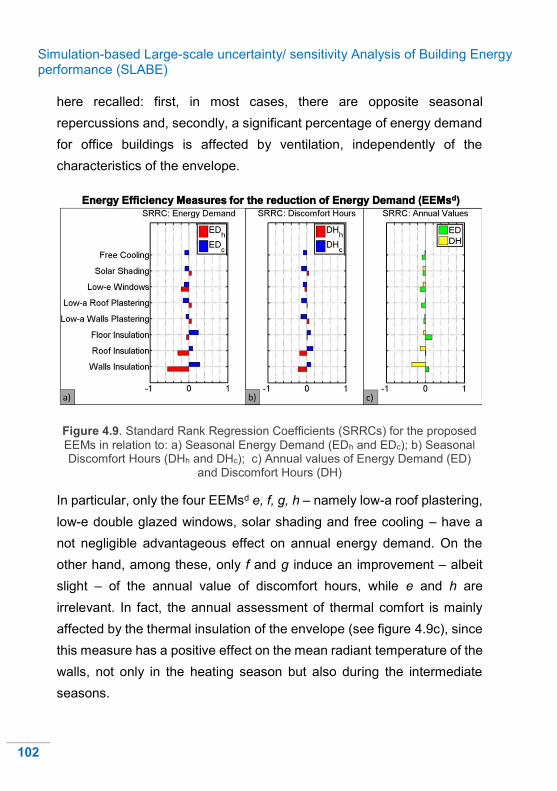
Simulation-based Large-scale uncertainty/ sensitivity Analysis of Building Energy performance (SLABE)
102
here recalled: first, in most cases, there are opposite seasonal
repercussions and, secondly, a significant percentage of energy demand
for office buildings is affected by ventilation, independently of the
characteristics of the envelope.
Figure 4.9. Standard Rank Regression Coefficients (SRRCs) for the proposed
EEMs in relation to: a) Seasonal Energy Demand (EDh and EDc); b) Seasonal Discomfort Hours (DHh and DHc); c) Annual values of Energy Demand (ED)
and Discomfort Hours (DH)
In particular, only the four EEMsd e, f, g, h – namely low-a roof plastering,
low-e double glazed windows, solar shading and free cooling – have a
not negligible advantageous effect on annual energy demand. On the
other hand, among these, only f and g induce an improvement – albeit
slight – of the annual value of discomfort hours, while e and h are
irrelevant. In fact, the annual assessment of thermal comfort is mainly
affected by the thermal insulation of the envelope (see figure 4.9c), since
this measure has a positive effect on the mean radiant temperature of the
walls, not only in the heating season but also during the intermediate
seasons.

Simulation-based Large-scale uncertainty/ sensitivity Analysis of Building Energy performance (SLABE)
103
4.3.2.2. Primary energy consumption and global cost (stage 2)
The achievable savings in PEC and GC compared to the current
configuration of the building stock are investigated. As described in
section 4.2.2, the exploration follows three steps:
step 3 contemplates the mere replacement of the primary heating/
cooling system ;
step 4 introduces the installation of renewable energy sources (RESs),
in particular PV panels;
step 5 introduces the implementation of EEMs for the reduction of
energy demand, in order to find the cost-optimal package of energy
retrofit actions.
For PEC evaluation the primary energy factor is set equal to 1 for natural
gas and to 2.18 for electricity, according to Italian standards. For GC
evaluation, a calculation period of 20 years is used, as prescribed by the
guidelines of the EPBD Recast for non-residential buildings. The prices
of electricity and natural gas, considered constant, are respectively set
equal to 0.25 €/kWhel and 0.90 €/Nm3 [116].
Replacement of the primary heating/cooling system (step 3)
The analysis of savings in PEC and GC is initially carried out considering
the mere replacement of the primary heating/cooling (HVAC) system.
Therefore, the sampling set S1 – which represents the existing building
stock – is considered in this stage. As aforementioned, the RefB is
characterized by a natural gas boiler (reference boiler: RB) and by an air-
cooled chiller (reference chiller: RC), while the proposed options for the
replacement of the system (see table 4.5) are listed below:
efficient boiler (EB), condensing boiler (CB), heat pump (HP) for
heating generation;

Simulation-based Large-scale uncertainty/ sensitivity Analysis of Building Energy performance (SLABE)
104
efficient air-cooled chiller (ACC), water cooled-chiller (WCC) for
cooling generation.
Thus, twelve configurations of the HVAC system are investigated,
including RB and RC. Figure 4.10 shows mean value and standard
deviation of the achievable PEC savings, in correspondence of these
configurations. Two different metrics are used: energy per building
[MWh/a] and energy per area [kWh/m2 a]. The second one is more used
in building applications and recommended by EPBD Recast, but the first
one is more appropriate for this study, because it allows a rapid estimation
of the potential PEC saving in the whole stock. Furthermore, figure 4.10
indicates that the trends are similar, so that the observations made for
energy per building are generally also valid for energy per area. Thus, the
second metric is used hereinafter. The adption of efficient systems can
induce significant energy savings in the stock, up to a mean value around
26 MWh/a per building (33 kWh/m2a) in presence of WCC and CB or HP
(see figure 4.10). The replacement of the cooling system ensures higher
potential savings, by virtue of the magnitude of cooling demand.
Figure 4.10. Mean Value and Standard Deviation of the of the achievable savings
in PEC for S1, in correspondence of the investigated HVAC configurations

Simulation-based Large-scale uncertainty/ sensitivity Analysis of Building Energy performance (SLABE)
105
More in detail, figure 4.11 shows the potential savings in PEC and GC,
respectively in presence of fan coils (figure 4.11a) and hot water radiators
(figure 4.11b). The results are analyzed separately for these two subsets
– characterized by 250 samples each – since the type of terminal highly
affects the performance of the heat generation system. The observations
on the cooling system are obviously the same for the two subsets, since
only a type of cooling terminal is considered, namely fan coils. The figure
confirms that both PEC and GC are highly influenced by the type of
cooling system, since the cooling demand is predominant for office
buildings in Naples. Thus, the best cooling system from both perspectives
is the most efficient one, which is the WCC. On the contrary, the
congruency between the two analyzed perspectives is not always
ensured as for the heating system, as argued below for the two subsets.
As expected, the presence of fan coils leads to higher values of energy
savings, mainly in correspondence of CB and HP, which ensure the
greatest savings in PEC. This occurs because of the lower temperature
of inlet hot water of fan coils compared to radiators. On the contrary, GC
savings are maximized by RB and EB. In fact, cost savings are ensured
for about 75% of buildings using one of these two boilers together with
the WCC, so that the probability that one of these two configurations will
be implemented is very high. In this way, the larger potential energy
savings guaranteed by CB and HP will be wasted. On the other hand, the
radiators induce lower values of energy savings and ergo cost savings.
The higher temperature of inlet hot water causes a deterioration of system
efficiency mainly for CB and HP. This leads to a greater congruence
between the energy and cost perspectives, in presence of radiators.
Indeed, the EB represents an optimal compromise, since it is very close
to both the best solutions respectively related to PEC (CB) and GC
savings (RB).
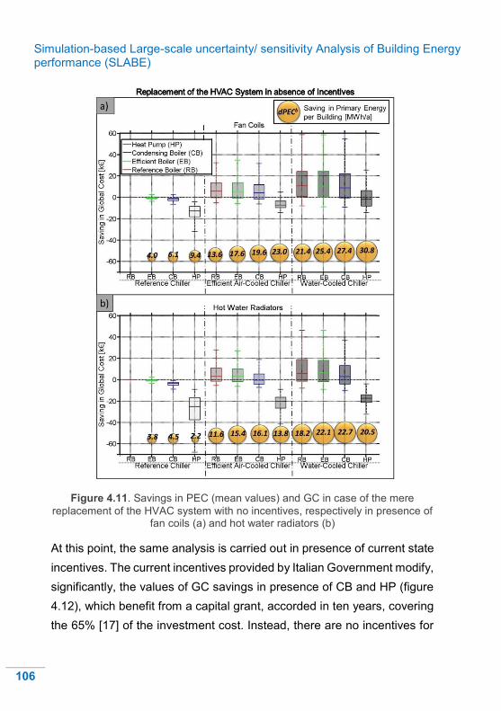
Simulation-based Large-scale uncertainty/ sensitivity Analysis of Building Energy performance (SLABE)
106
Figure 4.11. Savings in PEC (mean values) and GC in case of the mere
replacement of the HVAC system with no incentives, respectively in presence of fan coils (a) and hot water radiators (b)
At this point, the same analysis is carried out in presence of current state
incentives. The current incentives provided by Italian Government modify,
significantly, the values of GC savings in presence of CB and HP (figure
4.12), which benefit from a capital grant, accorded in ten years, covering
the 65% [17] of the investment cost. Instead, there are no incentives for

Simulation-based Large-scale uncertainty/ sensitivity Analysis of Building Energy performance (SLABE)
107
cooling systems, so that the WCC remains the best solution from all the
points of view. Thus, the attention is hereinafter focused on the heating
system. Obviously the values of PEC savings do not change compared
to the case of absence of incentives.
Figure 4.12. Savings in PEC (mean values) and GC in case of the mere
replacement of the HVAC system with current incentives, respectively in presence of fan coils (a) and hot water radiators (b)
Simulation-based Large-scale uncertainty/ sensitivity Analysis of Building Energy performance (SLABE)
108
The cost-optimal HVAC system is composed by WCC and CB, both in
presence of fan coils (figure 4.12a) and radiators (figure 4.12b), while the
highest PEC savings occur in correspodence of WCC–HP for fan coils
and WCC–CB for radiators. Thus, current incentives are fine in the case
of radiators since the two solutions match, but they are not effective in the
case of fan coils, because they don’t support enough the heat pumps: in
fact, the CB – which ensures a higher money saving – will be preferred
in most cases.
Therefore, this study tests a different incentive strategy in order to get
more satisfactory results. It consists of a capital grant, accorded in ten
years, that covers:
the 70% of the investment cost of heat pumps, if the building is heated
by fan coils;
the 65% of the investment cost of new efficient boilers, if the building
is heated by radiators.
Condensing boilers are not contemplated. This strategy aims at the
following objectives:
to encourage the use of heat pumps in presence of fan coils, since
they induce huge energy savings;
to encourage the use of new efficient boilers in presence of radiators;
this heating system is preferred to the condensing boiler, because –
compared to the latter – it induces a just slightly smaller energy saving,
in spite of a much lower investment cost.
The new values assumed by GC savings for fan coils and radiators are
depicted in figure 4.13. As expected, the best heating system with
proposed incentives is HP in presence of fan coils and EB in presence of
radiators. Thus, the harmonization between the two perspectives is
ensured.
Therefore, the cost-optimal HVAC systems consist of:

Simulation-based Large-scale uncertainty/ sensitivity Analysis of Building Energy performance (SLABE)
109
WCC in all cases;
CB in presence of current incentives, in both cases of fan coils and
radiators;
HP in case of fan coils and EB in case of radiators, in presence of
proposed incentives
Figure 4.13. Savings in PEC (mean values) and GC in case of the mere
replacement of the HVAC system with proposed incentives, respectively in presence of fan coils (a) and hot water radiators (b)

Simulation-based Large-scale uncertainty/ sensitivity Analysis of Building Energy performance (SLABE)
110
All told, the two strategies of current and proposed incentives for HVAC
systems are compared in table 4.6, through the indicators (p, dPECb, Db,
π), described in section 4.2.2. It is recalled that such indicators are
evaluated in the assumption that only the cost-optimal HVAC system
(which ensures the best values of GC savings) can be implemented.
Table 4.6 Comparison between current and proposed incentive strategies,
directed to the mere replacement of the HVAC system
Proposed incentives are penalized by the highest value of actual state
disbursement Db – due to the substantial support to heat pumps –
resulting in a lower value of the state profit π; in spite of this, they ensure
a higher actual energy saving dPECb (5.6% more) and they encourage
the spread of heat pumps, stimulating the reduction of the investment cost
of this efficient system. Thus, in the long term, proposed strategy appears
more effective.
RESs: Installation of PV Panels (step 4)
Once the best configurations of the primary heating/cooling system are
identified, the implementation of PV panels is investigated. At first, the
savings in PEC and GC are assessed in presence of RB and RC, in
function of the percentage of PV power (area fo PV panels) compared to
the maximum installable power (maximum area) on the buildings’ roofs.
In particular, these savings are represented in figure 4.14, in the cases
of:
REPLACEMENT OF
THE HVAC
SYSTEM p
dPECb MWh/a per
building
Db k€ per
building
π kWh/€
CURRENT INCENTIVES
0.79 19.8 5.63 3.52
PROPOSED
INCENTIVES 0.78 20.9 6.97 3.00

Simulation-based Large-scale uncertainty/ sensitivity Analysis of Building Energy performance (SLABE)
111
absence of incentives (figure 4.14a);
presence of current state incentives, which cover (in ten years) the
50% [17] of the investment cost for PV panels (figure 4.14b);
presence of proposed incentives, which cover (in ten years) the 40%
of the investment cost for PV panels (figure 4.14c).
Figure 4.14. Savings in PEC (mean values) and GC in function of the percentage of
PV power compared to the maximum installable power, in presence of RB and RC, respectively with no incentives (a), current incentives (b), proposed incentives (c)

Simulation-based Large-scale uncertainty/ sensitivity Analysis of Building Energy performance (SLABE)
112
The implementation of PV maximum power induces huge energy savings
– an average of 38.5 MWh/a per building – but it’s very likely that, in
absence of incentives, most buildings will install only a limited part (20-
30%) of the available power, in order to achieve a major money saving.
Thus, incentives are necessary to harmonize the two so-far-examined
perspectives. However, current incentives are excessive. Indeed, the
proposed ones are sufficient to support the implementation of the
maximum PV power, by ensuring positive values of the saving in GC for
the whole building stock. Therefore, the best option from both private and
collective perspectives is the installation of the maximum PV power
(100%), with both current and proposed incentives.
As regards the explored building category, the greatest part of electricity
produced by the PV panels is absorbed by lights and electrical
equipment, since these provide a significant energy demand in office
buildings. That’s why, in this case study, the replacement of the HVAC
system and the implementation of PV panels can be considered as
independent from an energetic point of view. In other words, in presence
of current and proposed incentives, the installation of the maximum PV
power represents the best option in correspondence of all the twelve
investigated HVAC configurations, as shown for the reference HVAC
system. Moreover, it induces similar GC savings for these HVAC
configurations. Thus, the cost-optimal combination of PV and HVAC
systems is provided by the installation of the maximum PV power and of
the cost-optimal HVAC option identified in the case of mere replacement
of the HVAC system.
More in detail, the following cost-optimal combinations are achieved:
in presence of current incentives: maximum PV power, WCC, CB
in both cases of fan coils and radiators;

Simulation-based Large-scale uncertainty/ sensitivity Analysis of Building Energy performance (SLABE)
113
in presence of proposed incentives: maximum PV power, WCC, HP in
presence of fan coils and EB in presence of radiators.
The savings in PEC and GC provided by these cost-optimal solutions are
depicted in figure 4.15.
Figure 4.15. Savings in PEC (mean values) and GC for the cost-optimal
configurations of HVAC system and PV panels (100%) in presence of current incentives (WCC+CB for fan coils and radiators) and proposed incentives
(WCC+HP for fan coils and WCC+EB for radiators)
Proposed incentives produce slightly lower GC savings for both kinds of
heat terminals. Nevertheless, they ensure money savings for almost the
whole building stock, as well: 96% of samples (against 99% in presence
of current incentives). On the other hand, the proposed strategy leads to
higher PEC savings for fan coils (~5% more) and similar PEC savings for
radiators compared to the current one. This rewards the devised choices
for incentives, by confirming that:

Simulation-based Large-scale uncertainty/ sensitivity Analysis of Building Energy performance (SLABE)
114
in presence of fan coils, heat pumps provide significant energy
savings;
in presence of radiators, new efficient boilers and condensing boilers
provide analogous energy savings; however the first ones are less
expensive and so more convenient.
In more detail, the two overall incentive strategies for HVAC and PV
systems are compared in table 4.7.
Table 4.7 Comparison between current and proposed incentive strategies,
directed to the replacement of the HVAC system and to the implementation of PV panels
They induce similar values of dPECb, but the proposed incentives lead to
a significantly lower Db and, consequently, to a higher profit π. Thus, the
proposed strategy better achieves the purpose of incentives, that is the
harmonization of private and collective interests.
Implementation of EEMsd (step 5)
As shown by SA, only four EEMsd have a positive impact on annual
energy demand (figure 4.9c), so that they can improve PEC and GC.
Thus, only these EEMsd are here considered. In particular, they consist
of:
e) low-a plastering of the roof;
f) installation of double-glazed low-e windows with PVC frame;
g) implementation of external shading of the windows;
REPLACEMENT OF
THE HVAC
SYSTEM + PV
PANELS
p dPECb
MWh/a per building
Db k€ per
building
π kWh/€
CURRENT INCENTIVES
0.99 62.7 44.6 1.41
PROPOSED
INCENTIVES 0.96 62.8 37.8 1.66

Simulation-based Large-scale uncertainty/ sensitivity Analysis of Building Energy performance (SLABE)
115
h) achievement of night free cooling, by means of mechanical ventilation.
It’s recalled that two sampling sets have been generated so far:
S1, representing the existing stock, characterized by 46 parameters
and 500 samples;
S2, representing the renovated stock in presence of the eight EEMsd,
characterized by 64 parameters and 500 samples.
At this point, a new sampling set S3 is needed to consider the
implementation of the 15 packages deriving from the combination of the
four aforementioned EEMsd e, f, g and h. Involved parameters are here
51, including 46 for buildings’ description, 4 (boolean parameters) for
EEMsd and 1 for shading set point. The exhaustive sampling of these 51
parameters generates the set S3 of 1500 samples, which are composed
of 15 groups of 100 samples. Each group corresponds to a EEMsd
package. 100 samples are sufficient to obtain reliable results in
correspondence of each package, since they ensure the stability of mean
value and standard deviation of energy demand and percentage of
discomfort hours. This occurs in correspondence of both S1 (see figure
4.3) and S2 (as verified by the authors), and so it must occur also for each
of the 15 groups of S3, since the latter presents a number of parameters
intermediate between S1 and S2. Hence, the potential savings of PEC and
GC refer to S3. At first, these savings are assessed for all the considered
pakages of EEMsd in correspondence of RB and RC, respectively:
in absence of incentives (figure 4.15a);
in presence of current incentives (figure 4.15b); among the considered
EEMsd, only the installation of low-e windows (EEMd f) is supported by
a capital grant that covers the 65% (in ten years) [17] of the investment
cost.
No incentives are proposed for the EEMsd because they are not effective,
as argued below.

Simulation-based Large-scale uncertainty/ sensitivity Analysis of Building Energy performance (SLABE)
116
Figure 4.15. Savings in PEC (mean values) and GC provided by the packages
of EEMsd in presence of RB and RC, respectively with no incentives (a) and current incentives (b)
The mere implementation of EEMsd packages induce lower PEC savings
compared to the other retrofit actions, because of the discussed
characteristics of the building category. The EEMd most affecting PEC is
the installation of low-e windows, followed by the solar shading, the roof
low-a plastering and the implementation of free cooling. This confirms the

Simulation-based Large-scale uncertainty/ sensitivity Analysis of Building Energy performance (SLABE)
117
results of the sensitivity analysis: the EEMsd with higher absolute values
of the SRRC related to annual energy demand (see figure 4.9c) have a
higher influence on PEC. This outcome is not obvious, since energy
demand causes only a part of PEC. In fact, the replacement of the
windows and the solar shading have very close values of the considered
SRRC but the first EEM is much more influential on PEC; this occurs
because solar shading induces an increase of energy comsumption for
lighting, which represents another part of PEC.
Although the installation of low-e windows is the EEMd that induces the
highest energy savings, it is not cost-effective in absence of incentives.
Instead, current incentives ensure GC savings for about the 50% of
buildings that implement only this energy measure. However, the
resulting PEC saving in the stock is much slighter than that produced by
new efficient HVAC systems and RESs. Thus, it doesn’t justify the huge
state disbursement required by such grants. For this reason, current
incentives addressed to new insulating windows are considered not
effective, in relation to the investigated building category.
The GC savings provided by the packages of EEMsd decrease with
increasing the number of measures. Most packages are not cost-effective
for the majority of explored samples. In particular, in presence of
incentives, only low-e windows, low-a roof and their combination ensure
cost savings for more than half of the samples. The cost-optimal package
includes only the low-a plastering of the roof, which induces cost savings
for the 75% of the stock.
Since the EEMsd have a slight influence on PEC compared to the
previous retrofit actions, their implementation does not alter the cost-
optimal combination of HVAC system and PV panels, which includes CB,
WCC and maximum PV power. Thus, the potential savings in PEC and
GC provided by the packages of EEMsd are calculated in correspondence

Simulation-based Large-scale uncertainty/ sensitivity Analysis of Building Energy performance (SLABE)
118
of such combination, applied to the building instances gathered in S3. The
outcomes, related to the existence of current incentives, are depicted in
figure 4.16.
Figure 4.16. Savings in PEC (mean values) and GC for the cost-optimal
combination of HVAC system (CB+WCC) and PV panels (100%), with current incentives, for the investigated packages of EEMsd
As anticipated, the mean increase of PEC saving per building (maximum
value of 8.9 MWh/a) is insignificant compared to the mean saving induced
by the replacement of the HVAC system and the implementation of PV
panels (63.3 MWh/a). This shows that the EEMsd don’t lead to substantial
energetic benefits, once improved the heating/cooling/electricity
generation system.
Furthermore, none of the EEMsd introduces evident GC savings, so that
the best choice for the buildings’ owners is to not implement them. Thus,
the cost-optimal package of energy retrofit actions for most buildings of

Simulation-based Large-scale uncertainty/ sensitivity Analysis of Building Energy performance (SLABE)
119
the stock is represented by the mere installation of the cost-optimal
combination of HVAC system and PV panels, namely CB, WCC and
maximum PV power.
Moreover, the considered incentives are not convenient from the
collective perspective, even in the hypothetical case that the replacement
of the windows is implemented, although this does not guarantee
sufficient GC savings. Indeed, these incentives determine a significant
state disbursement (~16 k€ per building), in spite of a small increase of
the mean value of PEC saving (~6 MWh/a per building). More in detail,
table 4.8 shows how the incentives directed to EEMd f affect the values
of p, dPECb, Db and π evaluated for the overall current incentive policy.
Table 4.8. Indicators of the overall current incentive strategy, respectively in
absence and in presence of incentives for the replacement of the windows
They cause an evident decrease of the state profit π, since the increase
of Db is much more significant than the increase of dPECb. It is clear that
the situation gets worse if such incentives are raised in order to more
encourage the single buildings, since dPECb remains constant (p=1)
while Db increases. Thus, state incentives for new windows are not
advantageous, and similar considerations are valid for the other EEMsd
aimed at the reduction of energy demand. In fact, the potential energy
savings induced by these measures are not such as to justify the state
intervention, as regards the investigated case study.
OVERALL
CURRENT INCENTIVES
p dPECb
MWh/a per building
Db k€ per
building
π kWh/€
NO INCENTIVES
FOR WINDOWS
0.99 62.7 44.6 1.41
INCENTIVES FOR WINDOWS
1.00 69.3 60.6 1.14

Simulation-based Large-scale uncertainty/ sensitivity Analysis of Building Energy performance (SLABE)
120
In conclusion, once improved the heating/cooling/electricity generation
system, the implementation of EEMsd is not convenient from both
collective and private perspectives. Thus, the proposed incentive strategy
doesn’t support such EEMsd, since the two perspectives don’t need to be
harmonized. These considerations are valid for office buildings in Naples
and in other localities of South Italy with similar climatic conditions, where
the energy demand for cooling is predominant.
Final remarks
All told, it is emphasized that the implementation of SLABE provides
worthy global indications on the cost-optimal package of energy retrofit
measures for a building category SLABE. However, the main weakness
of the methodology is the impossibility of obtaining detailed information
on the cost-optimality of retrofitting each single building. This has led to
the development of ANNs that exploit the outcomes of UA and SA
performed in SLABE, as discussed in the next chapter.

Artificial Neural Networks (ANNs) for the prediction of building energy performance
121
How to evaluate the global cost of a building with
a minimum computational time and a good reliability?
CHAPTER 5. Artificial Neural Networks (ANNs) for the prediction of building energy performance
5.1. Introduction
The cost-optimal analysis prescribed by the EPBD Recast is a
computationally expensive procedure, because it requires several
transient energy simulations, generally performed in BPS tools. This
results in a large amount of the required computational time that can
assume an order of magnitude from days, for simple buildings, until
months, for quite complex ones. This chapter aims to handle this issue
by proposing the development of surrogate models, i.e. artificial neural
networks (ANNs), for the assessment of building energy performance.
The benefit is represented by a substantial reduction of computational
time and complexity.
A surrogate model (or meta-model) is a “model of the model” [117], that
is a function of the design variables that emulates a more complex one,
generally based on expensive computer models, thereby approximating
the objective functions (Sacks et al. 1989). The surrogate models are built
from the data gathered in several evaluations of the objective functions
realized by means of the original model. Therefore, their development
involves a long procedure. However, once built, the meta-model is highly
advantageous, because, compared to the original one, it is much faster
in the evaluation of the objectives. Common meta-modeling techniques

Artificial Neural Networks (ANNs) for the prediction of building energy performance
122
are Multivariate Adaptive Regression Splines (MARS), Kriging (KG),
Radial Basis Function (RBF), Artificial Neural Networks (ANNs), and
Support Vector Regression (SVR). A crucial issue in meta-modeling is the
selection of a proper surrogate model type under a given condition.
The most used techniques for the prediction of the energy and thermal
behavior of buildings are, essentially, KG [118, 119], SVR [83, 123, 124]
and ANNs [81,125-140] that represent the most popular method. In
several cases, such meta-models are adopted for replacing a BPS tool
inside an optimization procedure, in order to reduce the computational
time. In this regard, an interested review and comparison of
metamodeling techniques for simulation optimization in Decision Support
Systems is provided by Li [141].
Actually, a perfect meta-model technique does not exist and the correct
choice depends on the characteristics of the problem. ANNs are
particularly widespread in the building sector because they ensure a good
performance with large-size problems, as those typical of building energy
studies. Concerning building applications, ANNs have been widely used
for the prediction of hourly energy demand for space conditioning [126-
133], daily heating and cooling load [134, 135], annual energy
consumption [81, 136, 137] and average thermal comfort (PMV) [81, 137,
138]. Furthermore, ANNs have been also used for modeling the energy
behavior of a whole building stock [139, 140], instead of single buildings.
In all mentioned cases, the networks ensure optimal performance, by
providing a regression coefficient (R) around (higher in most cases to)
0.9.
It is emphasized that the development of meta-models for the evaluation
of building energy performance is a long and critical process, since it
requires several simulations performed through BPS tools. That’s why the
generation of surrogate models that are valid merely for a single building

Artificial Neural Networks (ANNs) for the prediction of building energy performance
123
is generally pointless, except for some cases characterized by the
implementation of optimization algorithms that needs a higher number of
BPS simulations, compared to that required by the surrogate models [81,
83, 118, 119, 137]. On the other hand, the generation of surrogate models
that can be used to investigate several buildings appears particularly
worthwhile. Indeed, in this case, the powerful capability of such models is
thoroughly exploited with a consequent huge benefit. A meta-model can
be compared to a Swiss knife. As the adoption of a Swiss knife is useful
only if most blades are used, so the development of a surrogate model is
worthwhile only if it can be fully exploited. In other words, if only one blade
is needed, a simple knife is more convenient, because less expensive;
similarly, if the energy behavior of a simple building should be
investigated, the use of BPS tools is generally more convenient, because
it ensures a higher accuracy and a lower computational cost.
Starting from this consideration, the methodology proposed in this
chapter consists in the generation of ANNs for the assessment of energy
consumption, thus global cost, and thermal comfort of any building
belonging to an established category, in absence and presence of energy
retrofit measures (ERMs). The ANNs are developed in MATLAB
environment, by using EnergyPlus outcomes, post-processed and
handled in MATLAB, as targets for training and testing the networks.
In the following lines, the methodology is first described and then applied
to the category explored in the previous chapter, namely office buildings
built in South Italy in the period 1920-1970.
Alike CAMO and SLABE, the developed ANNs can be adopted either as
a stand-alone tool or as a part (stage II) of the macro-methodology
(CASA) proposed in this thesis (see chapter 6).

Artificial Neural Networks (ANNs) for the prediction of building energy performance
124
5.2. Methodology
The methodology is based on the use of ANNs for the simulation of
building energy and thermal behavior. Artificial neural networks have
been chosen among the aforementioned meta-modeling techniques, for
two main reasons, reported also in [81]: firstly, they have shown their
efficiency and strong capability in a number of previous studies on
building energy performance [81,125-140]; secondly, they are pre-
programmed in many programs, such as MATLAB.
An ANN is a processing data system that learns the relationship between
inputs and outputs by studying previously recorded data, obtained from
the original model. It consists in a “network of elementary computation
units called neurons, as a reference to the human brain function” [142].
The neurons are connected to each other by a number of weighted links,
denoted as synaptic connections (synapses), over which information is
transmitted and manipulated. Each neuron receives input data from the
previous ones by means of synapses, handles such data and combines
them, through a transfer function, in order to generate output data that
are sent to the following neurons. The net learns from the provided inputs
and outputs through the training. More in detail, the training is an iterative
procedure that is finalized to properly set the weights of the synaptic
connections, by optimizing a certain parameter, for instance the sum of
squared errors (SSE) [81] or the root mean squared error (RMSE) [137].
The training is stopped when a criterion is satisfied; for example, when an
established maximum number of iterations, denoted as epochs, is
reached (no-stop training method).
The most popular and simple ANN architecture is the feed-forward multi-
layer perceptron (MLP), which is characterized by the presence of
different neuron layers: one input layer, one or many hidden layers and
one output layer (see figure 5.1). The input layer receives data

Artificial Neural Networks (ANNs) for the prediction of building energy performance
125
(independent variables) from outside, while the output layers provides the
outcomes (objective functions) of the net. Between these two layers, a
network can have one or more intermediate hidden layers. The number
of such layers should be properly chosen: too many hidden layers lead to
an over-fitting of the model; not enough layers can hinder the robustness
and reliability of the ANN learning process [136].
Figure 5.1. Architecture of a feed-forward multi-layer ANN, with one hidden layer
The performance of an ANN significantly depends on input and output
data, as well as on its architecture and parameters [136], which must be
chosen carefully.
The ANN model used in this study is a feed-forward MLP, composed of
three layers and thus with only one hidden layer. The number of hidden
neurons is detected by trial-and-error. This parameter highly influences
the ANN performance: when it increases, the training data set error
decreases at the cost of compromising the generalization ability of the
model. The network is trained with Levenberg–Marquardt back-
propagation algorithm coupled with Bayesian regularization. A sigmoidal

Artificial Neural Networks (ANNs) for the prediction of building energy performance
126
function for the hidden layer and a linear function for the output layer are
used as transfer function. A similar configuration of the net has been
adopted in previous worthwhile building studies with optimal results [81,
133, 137, 139, 140]. The training of the ANN is stopped when either the
RMSE stabilizes over a certain number of epochs or the maximum
number of epochs, set equal to 1000 as in [133], is reached. Then, the
network is tested on a second sample of input and output data by
considering as performance indicators the coefficient of regression (R)
and the distribution of the relative error between the ANN outputs and the
‘original’ ones. EnergyPlus simulations provide the data that, after a post-
process in MATLAB, are exploited for ANN training and testing. The
number of samples gathered in the training set should be selected
properly according to architecture and dimensions of the network; for
instance, according to Conraud [143], the minimum value of this number
for achieving reliable results is equal to 5 × number of inputs × number of
outputs. The ratio between the sizes of training and testing sets is set
equal to 9/1 in agreement with previous studies [81, 137]
By adopting the described ANN model, two families of networks are built
in order to assess energy performance and thermal comfort of each
building belonging to an established category. The first family refers to
the existing building stock, whereas the second one refers to the
renovated stock, in presence of well-selected ERMs.
More in detail, the first family of ANNs consists of three independent
networks, all characterized by a single output, finalized to assess
respectively:
the primary energy demand for heating (ANN for EPh [kWh/m2 a]);
the primary energy demand for cooling (ANN for EPc [kWh/m2 a]);

Artificial Neural Networks (ANNs) for the prediction of building energy performance
127
the percentage of annual discomfort hours as defined in section 3.2.1
(ANN for DH [%]).
The inputs of the networks are represented by the parameters, related to
the whole ‘building system’, that affect the considered outputs. These
parameters can concern building geometry, envelope, operation and
HVAC system. The three ANNs are developed and verified by using the
same training and testing sets, whose size is imposed by the network with
more inputs (characterized by the highest value of the minimum
acceptable size of the training set). The use of different networks with
only one output neuron, instead of a single network with more output
neurons, determines a reduction of the computational burden required by
the nets’ learning, as well as an improvement of meta-modeling reliability,
as suggested by Boithias et al. [144]. Indeed, if a single ANN with three
outputs – namely EPh, EPc, and DH – is used, all the parameters that
influence one or more of these three objectives should be included in the
(unique) group of the ANN’s inputs. Diversely, if three independent ANNs
are used, three smaller groups of inputs, chosen ad ‘hoc’ in
correspondence of each output, can be adopted. This induces a reduction
of the required size of the training set, compared to the case of a single
ANN, and thus a lower computational burden. Indeed, the number of
EnergyPlus simulations, needed for the nets’ training, decrease, with a
consequent shortening of the most computationally-expensive phase of
the procedure. Furthermore, the generation of independent ANNs for the
three outputs ensures higher reliability, because only the parameters that
actually affect a certain output are considered as inputs of the network
associated to that output. In this regard, EPh and EPc have been
preferred, as ANNs’ outputs, to the total primary energy demand for space
conditioning (EP = EPh + EPc) because there are some building
parameters (e.g., the heating set point temperature) that affect EPh

Artificial Neural Networks (ANNs) for the prediction of building energy performance
128
without influencing EPc, and viceversa (e.g., the cooling set point
temperature). Therefore, this choice allows to reduce the number of the
nets’ inputs, with the aforementioned benefits.
The final goal of the ANNs is to provide, besides DH, the primary energy
consumption (PEC [kWh/a]) and the global cost (GC [€]) for any building
of the category. In particular, diversely from chapter 4, here and in the
next chapter, the PEC per unit of conditioned area, denoted with PEC’
[kWh/m2 a], is considered, since this metric is more suitable when the
interest is focused on the energy saving achieved for whichever building
and not for the whole stock. PEC’ and GC are calculated by means of a
post-process performed in MATLAB. It is recalled that PEC’ doesn’t
include only EPh and EPc, but also energy consumption for DHW (EPdhw
[kWh/m2 a]) and electric uses (EPel [kWh/m2a]). In this study, EPdhw and
EPel are evaluated in MATLAB, in a simplified manner, by considering
typical schedules of DHW and electricity demand. The author opted for
this choice because the interest is focused on the impact of some ERMs
on building energy performance; generally, a reliable quantification of
such impact on EPdhw and EPel does not need the use dynamic energy
simulations with BPS tools. Nevertheless, in more complex cases, further
ANNs for the evaluation of EPdhw and EPel can be developed.
Similar considerations are valid for the assessment of GC, which is
calculated according to the guidelines of the EPBD Recast. It is noted
that, in addition to the aforementioned motivation, the choice of setting
EPh and EPc as ANNs’ outputs, instead of EP, also derives from the will
of evaluating the global cost. Indeed, the procedures for deriving the
operating cost, respectively for space heating and space cooling, from
the primary energy consumption can differ, because different conversion
systems can be used. A typical example is represented by the presence
of a gas boiler for heating end of an electric chiller for cooling.

Artificial Neural Networks (ANNs) for the prediction of building energy performance
129
The second family of ANNs consists of other four independent networks,
related to the renovated building stock, characterized by a single output
because of the reasons previously argued and finalized to assess
respectively:
the primary energy demand for heating (ANN for EPh [kWh/m2 a]);
the primary energy demand for cooling (ANN for EPc [kWh/m2 a]);
the percentage of annual discomfort hours (ANN for DH [%]);
the thermal/ electric energy produced by in-situ renewable energy
sources (RESs) and consumed by the facility (ANN for ERES
[kWh/m2a]).
This family includes one more network, compared to the first one, in order
to take into account the energy produced by in situ RES systems, e.g.,
photovoltaic (PV) generators and solar thermal collectors, and consumed
by the building on the basis of hourly energy balances. This ANN is
introduced because the implementation of RESs represents a possible
ERM, which is very influential on building energy performance.
The four new ANNs aim to investigate the applications of ERMs.
Therefore, the inputs of the networks include both the parameters that
define the energy performance of existing buildings – i.e., the inputs of
the first three ANNs – and the parameters describing the energy retrofit
measures. As previously explained for the first family of networks, here
too, the four ANNs are independent. Indeed, they accepts different
groups of inputs in order to optimize and speed up the generation of such
surrogate models.
PEC’ and GC are derived from as previously explained, by taking into
account also the amount of energy that is produce by RESs and
consumed by the facility.

Artificial Neural Networks (ANNs) for the prediction of building energy performance
130
Finally, it is emphasized that a rigorous implementation of the proposed
methodology requires the combination with SLABE (see chapter 5), as
shown in the application reported below. Indeed, SLABE allows to carry
out a propaedeutic investigation of an established building category by
means of uncertainty and sensitivity analysis. Such procedure yields the
detection of the most influential parameters on each output of the seven
described ANNs, concerning both the current configuration of the stock
and the proposed ERMs. Thus, these parameters are used as networks’
inputs, thereby ensuring the aforementioned benefits produced by a
proper, ‘ad hoc’ development of each ANN.
5.3. Application
5.3.1. Presentation of the case study
The methodology is applied for exploring the energy and thermal behavior
of the buildings that belong to the category investigated by means of
SLABE in chapter 4, namely: Office buildings built in South Italy in the
period 1920-1970. For a detailed description of the case study the
readers are invited to refer to the section 4.3.1, which outlines the
characteristics of the examined buildings as well as the proposed ERMs.
The information gathered by means of SLABE allows to optimize the
development of the seven ANNs, three for defining the existing building
stock and four for assessing the impact of ERMs. It is recalled that the
energy and thermal behavior of the existing stock is defined by 46
parameters (see table 4.3): 9 for geometry, 30 for envelope and 7 other
parameters. They are assumed as the most affecting thermal energy
demand and comfort. In order to contemplate also the primary energy
systems, two additional parameters are here considered, namely the
efficiency (η) of the heating primary system (parameter p65) and the

Artificial Neural Networks (ANNs) for the prediction of building energy performance
131
energy efficiency ratio (EER) of the cooling primary system (parameter
p66). The energy conversion systems are, respectively, set equal to a gas
hot water boiler and to an air-cooled chiller, because these represent the
most popular HVAC configurations in the explored building stock. In order
to cover the vast majority of such stock, the boiler η (based on the low
calorific value) is varied within the range 0.7÷0.9, whereas the chiller EER
is varied within the range 1.5÷3. The two referred-to parameters are taken
into account in ANNs’ development for ensuring a more accurate and
reliable estimation of primary energy consumption and global cost for
each building of the stock. Indeed, the efficiency of the HVAC system is
a very influential parameter on the mentioned outputs. Diversely, SLABE
did not considered the variation of the two parameters, because it did not
aim to the analysis of each building, but to the achievement of global
indications for the cost-optimality of retrofitting the whole category.
Therefore, the adoption of average values for these parameters ensured
satisfying and reliable outcomes. Finally, the existing building stock is
represented by 48 parameters. Among these, the parameters that
exercise a non-negligible influence on each output of the three ANNs,
respectively for the assessment of EPh, EPc, and DH, are detected. In
particular, if the sensitivity index, namely the standardized rank
regression coefficient (SRRC) evaluated in section 4.3.2, is less than
0.05, the parameter is considered negligible on the output and ignored in
the generation of the corresponding ANN. This threshold value has been
chosen by observing a cutoff in the number of influential parameters vs.
the sensitivity index amplitude, as also done in [103]. It should be noted
that the SRRCs have been calculated, in chapter 4, in reference to the
demand of thermal energy (ED) and not of primary energy (EP). However,
this does not prejudice the reliability of the procedure, since a parameter
that is not negligible for ED, reasonably, will be not negligible for EP too.

Artificial Neural Networks (ANNs) for the prediction of building energy performance
132
This screening leads to the establishment of three groups of significant
parameters, used as inputs in the development of the three mentioned
ANNs. These groups are outlined in table 5.1.
The same procedure is applied for identifying the inputs of the four ANNs,
representing the renovated stock, in presence of ERMs. Among these,
the unique RES system consists of PV panels, and thus the denotation
ERES is replaced with EPV, in order to indicate the electricity produced by
the photovoltaic generators and consumed by the building.
The renovated building stock is characterized by 64 parameters (see
table 4.3 and 4.4). Specifically, in addition to the 46 ones describing the
existing buildings, there are eight boolean parameters (one for each ERM
for the reduction of energy demand), nine parameters related to the
characteristics of thermal insulants and one parameter related to the
shading set point. However, here, the thicknesses of the thermal insulants
are varied in the range 0÷12 cm, whereas in the application of SLABE,
they were fixed for ensuring the U values prescribed by Italian law to
obtain state incentives [17]. The upper value of the range, i.e., 12 cm, has
been established by virtue of local construction standards that take into
account the strong impact of energy demand for space-cooling in the
Mediterranean area, among all for office buildings, which are
characterized by a significant internal heat gain. Indeed, too high values
of insulant thickness would induce an increment of EP, caused by a
strong increase EPc, as also shown in chapter 3. The insulation thickness
is considered variable in the networks’ development, because this
parameter can highly affect both energy demand and thermal comfort.
Diversely, it has been considered fixed in the implementation of SLABE
in order to facilitate the interpretation of the results.
Therefore, the Boolean variables encoding the presence/ absence of the
insulation are replaced by continuous variables representing the

Artificial Neural Networks (ANNs) for the prediction of building energy performance
133
thickness of the insulation layers. This choice is justified, again, by the
different aims of the methodologies, consisting of the detailed analysis of
each building and retrofit action for the ANNs, and of a global investigation
of the building category for SLABE. Of course, the two additional
parameters (p65 and p66) that refer to the primary energy systems are
considered also in this case. Their ranges of variability should include
both the presence of existing and new efficient devices. Most notably, the
application of SLABE (see section 4.3.2) showed that the largely most
effective retrofit measures directed to the HVAC system consist of the
implementation of a condensing boiler (η = 1.06) and of a water-cooled
chiller (EER = 4.5). Hence, only these options are included in the in ANNs’
development, in such a way that the range of variability is set equal to
0.7÷0.9; 1.06 for boiler η and to 1.5÷3; 4.5 for chiller EER. Eventually, a
last parameter is introduced (p67) in order to express the percentage of
the building roof covered by polycrystalline PV Panels. As argued in
section 4.3.1, they are selected as RES because solar energy is one of
the most advantageous RESs in Europe [114], and particularly in Italy
because of favorable climatic conditions. PV panels are preferred to solar
thermal, because they are more cost-effective [72], in particular for office
buildings. In this study, they are characterized by 34° tilt angle and 0°
azimuth angle (orientation to south), in order to achieve the maximum
annual production of electricity, as verified bt means of PV-GIS Software
[115]. They have conversion efficency equal to 14%.
Finally, the renovated building stock is represented by 67 parameters.
Among these, the non-negligible parameters on each output of the four
ANNs, respectively for the assessment of EPh, EPc, DH, and EPV, are
detected by using the previously explained procedure, in which the
threshold value for the SRRC is set equal to 0.05. The resulting four
groups of ANNs’ inputs are outlined in table 5.2.

Artificial Neural Networks (ANNs) for the prediction of building energy performance
134
Table 5.1. Parameters selected as ANNs’ inputs for the existing building stock
PARAMETERS ANN FOR EPh ANN FOR EPc ANN FOR DH
GE
OM
ET
RY
p1 Orientation (North Axis) ● ● ●
p2 Area of each Floor [m2] ● ● ●
p3 Form Ratio ● ●
p4 Floor Height [m] ● ● ●
p5 Window to Wall Ratio: S ● ● ●
p6 Window to Wall Ratio: E ● ● ●
p7 Window to Wall Ratio: N ● ●
p8 Window to Wall Ratio: W ● ● ●
p9 Number of Floors ● ● ●
EN
VE
LO
PE
p10 Air Gap RT [m2 K/W]
p11 Roof a ● ● ●
p12 External Walls a ● ● ●
p13 Thickness of Concrete
[m]
p14 Type of Glass ● ●
p15 Type of Frame
p16 Clay t [m] ●
p17 Clay k [W/m K] ●
p18 Clay d [kg/m3]
p19 Clay c [J/kg K]
p20 Expanded Clay t [m]
p21 Expanded Clay k [W/m K]
p22 Expanded Clay d [kg/m3]
p23 Expanded Clay c [J/kg K]
p24 External Brick t [m] ● ● ●
p25 External Brick k [W/m K] ●
p26 External Brick d [kg/m3]
p27 External Brick c [J/kg K]
p28 Floor Block t [m]
p29 Floor Block k [W/m K]
p30 Floor Block d [kg/m3]
p31 Floor Block c [J/kg K]
p32 Internal Brick t [m] ● ●
p33 Internal Brick k [W/m K] ●
p34 Internal Brick d [kg/m3]
p35 Internal Brick c [J/kg K]
p36 Roof Block t [m] ●
p37 Roof Block k [W/m K] ●
p38 Roof Block d [kg/m3]
p39 Roof Block c [J/kg K]
OT
HE
R
p40 People Density [peop./m2] ● ●
p41 Light Load [W/m2] ● ●
p42 Equipment Load [W/m2] ● ●
p43 Infiltration Rate [h-1] ●
p44 Heating Set Point T [°C] ● ●
p45 Cooling Set Point T [°C] ● ●
p46 Heating Terminals ● ●
HV
AC
p65 Boiler η (0.7 ÷ 0.9) ●
p66 Chiller EER (1.5 ÷ 3) ●

Artificial Neural Networks (ANNs) for the prediction of building energy performance
135
Table 5.2. Parameters selected as ANNs’ inputs for the renovated building stock
PARAMETERS ANN FOR EPh ANN FOR EPc ANN FOR DH ANN FOR EPV
GE
OM
ET
RY
p1 Orientation (North Axis) ● ● ●
p2 Area of each Floor [m2] ● ● ●
p3 Form Ratio ● ● ●
p4 Floor Height [m] ● ● ●
p5 Window to Wall Ratio: S ● ● ●
p6 Window to Wall Ratio: E ● ● ●
p7 Window to Wall Ratio: N ● ● ●
p8 Window to Wall Ratio: W ● ● ●
p9 Number of Floors ● ● ● ●
EN
VE
LO
PE
p11 Roof a* ● ● ●
p12 External Walls a ● ● ●
p14 Type of Glass** ● ● ●
p16 Clay t [m] ●
p17 Clay k [W/m K] ●
p24 External Brick t [m] ● ●
p25 External Brick k [W/m K] ●
p32 Internal Brick t [m] ● ● ●
p33 Internal Brick k [W/m K] ●
p36 Roof Block t [m] ●
p37 Roof Block k [W/m K] ●
OT
HE
R
p40 People Density [peop./m2] ● ●
p41 Light Load [W/m2] ● ●
p42 Equipment Load [W/m2] ● ●
p43 Infiltration Rate [h-1] ●
p44 Heating Set Point T [°C] ● ●
p45 Cooling Set Point T [°C] ● ●
p46 Heating Terminals ● ●
EE
Ms
d
p47 Walls Insulation (tv = 0 ÷ 12 cm)
● ● ●
p48 Roof Insulation (tr = 0 ÷ 12 cm)
● ● ●
p49 Floor Insulation
p50 Low-a Plastering of the Walls ● ● ●
p51 Low-a Plastering of the Roof* ● ● ●
p52 Low-e double Windows** ● ● ●
p53 External Solar Shading ● ● ●
p54 Free Cooling ● ●
p55 - p64 Additional parameters
HV
AC
p65 Boiler η (0.7÷9; 1.06) ●
p66 Chiller EER (1.5÷3; 4.5) ●
RE
S
p67
Percentage of the Roof
covered by polycrystalline PV Panels (0 ÷ 100 %)
●
*The low-a plastering of the roof is contemplated by means of the variation of the roof a ** The low-e windows are contemplated by means of the variation of the type of glass

Artificial Neural Networks (ANNs) for the prediction of building energy performance
136
5.3.2. Results and discussion
All the developed networks are characterized by ten hidden neurons,
because this number ensures a good compromise between accuracy and
generalization ability of the models for the investigated case study.
Existing building stock
Three ANNs are developed for simulating the performance of the existing
building stock, respectively for the assessment of EPh, EPc, and DH. For
training and testing these networks, the sampling set S1 of 500 building
instances, generated by means of Latin Hypercube Sampling (LHS) for
the application of SLABE (see section 4.3.2), is considered. More in
detail, the performed EnergyPlus simulations, have provided for each one
of the mentioned 500 samples the following relevant data:
the hourly values of the predicted mean vote (PMV) for all the thermal
zones for the building;
the hourly values of thermal energy demand for heating and cooling.
From the values of PMV, the target DH is calculated in MATLAB.
Diversely, the evaluation of EPh and EPc requires an intermediate step,
since the LHS that leads to S1 involves only the parameters affecting the
demand of thermal energy (from p1 to p46), thereby not considering those
related to the primary energy systems (p65 and p66). Therefore, a further
LHS is needed in order to sample the parameters p65 and p66. In other
words, two sets of 500 values respectively of boiler η and chiller EER are
generated. Such values are used in order to obtain the values of EPh and
EPc from the hourly values of thermal energy demand provided by
EnergyPlus. This post-process is performed in MATLAB.
Eventually, a set of 500 values is achieved for each output, i.e., EPh, EPc
and DH, thereby representing the targets of the three respective ANNs.
The training set is composed of 450 cases (90% of cases), fulfilling the

Artificial Neural Networks (ANNs) for the prediction of building energy performance
137
minimum value proposed by Conraud [143], randomly picked from the
500 available samples. The testing test includes the remaining 50 ones.
The performance of the networks are evaluated by considering the
regression as well as the distributions of the relative errors between
ANN’s outputs and targets provided by EnergyPlus. The outcomes of the
testing are summarized in table 5.3 and in figure 5.2.
Table 5.3. Testing of the developed ANNs related to the existing building stock
ANNS EPOCHS R NUMBER OF CASES WITH RELATIVE ERROR AVERAGE
|RELATIVE
ERROR| <1% <2.5% <5% <10% <25%
EX
IST
ING
ST
OC
K
EPh 387 0.982 18 26 50 76 100 6.1%
EPc 336 0.975 10 22 44 76 100 6.9%
DH 394 0.966 12 18 38 70 100 8.4%
The average relative errors are quite good, respectively 6.1% for EPh,
6.9% for EPc and 8.4% for DH. The ANN for DH prediction is less accurate
because the estimation of thermal comfort is ruled by more complicated
phenomena, which are hardly predictable (e.g., radiation heat transfer
between walls and people, heat transfer between heating terminals and
people, and so on). The same conclusion was provided by previous
studies on the adoption of ANNs for the simulation of building energy
performance [81, 137]. It should be noticed that the values of relative
errors between ANNs’ outputs and targets are globally higher compared
to those achieved in similar worthy studies referred to a single building
[81, 137], since the analysis of a building stock is obviously much more
complicated, because of much wider ranges of parameters’ variability. On
the other hand, a similar approach for the investigation of energy and
thermal behavior of a whole building category is quite new; thus, the
current scientific literature does not provide many comparable studies for
a deeper investigation of the goodness of the proposed methodology.

Artificial Neural Networks (ANNs) for the prediction of building energy performance
138
The regressions between the ANNs’ predictions and the simulated targets
(see figure 5.2), also show a good agreement with regression coefficients
(R) very close to 1.
Figure 5.2. Meta-models of the existing building stock. ANNs vs EnergyPlus:
regression between ANNs’ outputs and simulated (EnergyPlus) targets and distributions of relative error

Artificial Neural Networks (ANNs) for the prediction of building energy performance
139
Renovated building stock
Four ANNs are developed for simulating the performance of the
renovated building stock, respectively for the assessment of EPh, EPc,
DH and EPV. For training and testing these networks, a new sampling set,
S4, is generated by means of LHS. The sample space is defined by the
parameters (and their correlated ranges) reported in table 5.2 that are
included in the inputs of at least one network, i.e. all the referred-to
parameters except for the floor insulation (p49) and the additional
parameters defining the ERMs (p55 - p64). The set S4 collects 1000 building
instances, which are run in EnergyPlus, by means of the coupling with
MATLAB. The outcomes of the simulations are post-processed in
MATLAB, as explained in the previous section, in order to achieve a set
of 1000 values for each output, i.e., EPh, EPc, DH and EPV, thereby
representing the targets of the four corresponding ANNs. By adopting the
aforementioned subdivision of the sampling set (90% vs 10%), the
training set is composed of 900 cases (fulfilling the minimum value
proposed by Conraud [143]), randomly picked, and the testing one
includes the remaining 100. A higher number of cases is used for the
developed of the ANNs, compared to the first networks’ family (existing
stock), because additional parameters are introduced for defining the
ERMs, which make the energy and thermal behavior of the buildings
much more heterogeneous. Thus, in order to ensure reliable outcomes
the number of cases is doubled.
The regression as well as the distributions of the relative errors between
ANN’s outputs and targets provided by EnergyPlus simulations are
summarized in figure 5.3 and in table 5.4.

Artificial Neural Networks (ANNs) for the prediction of building energy performance
140
Figure 5.3. Meta-models of the renovated building stock. ANNs vs EnergyPlus

Artificial Neural Networks (ANNs) for the prediction of building energy performance
141
Table 5.4. Testing of the developed ANNs related to renovated building stock
ANNS EPOCHS R NUMBER OF CASES WITH RELATIVE ERROR AVERAGE|
RELATIVE
ERROR| <1% <2.5% <5% <10% <25%
RE
NO
VA
TE
D
ST
OC
K
EPh 695 0.980 6 21 36 75 100 8.0%
EPc 655 0.979 7 22 37 76 100 8.1%
DH 384 0.960 11 17 33 54 90 11%
PV 479 0.997 60 75 85 96 100 2.0%
The performance of this second family of networks for EPh, EPc and DH
is quite similar, albeit a slight worsening, to that of the first family. Indeed,
the average absolute relative errors are respectively equal to 8.0% for
EPh, 8.1% for EPc and 11% for DH, as well as the regression coefficients
are lower, but still very close to one. This outcome is quite obvious
because the ANNs related to the renovated stock aim to predict the
behavior of a more complex, wide and various system. As already argued,
the ANN for DH assessment is the one with the worst performance. On
the other hand, the fourth network, that is the one for the prediction of
EPV, behaves very well (R = 0.997, average absolute relative errors =
2.0%) because it is characterized by only three inputs, consisting of
building form ratio, number of floors and percentage of the roof covered
by polycrystalline PV panels. The first two parameters affect the ratio
between the electricity produced by the PV generator and that required
by the facility, and thus the percentage of the produced energy that is
consumed, while the third parameter obviously exercises a huge
influence on the absolute value of electricity produced by the PV
generator.
In order to perform a further verification of the reliability and accuracy of
the two networks’ families, both of them are applied for predicting the

Artificial Neural Networks (ANNs) for the prediction of building energy performance
142
performance of the reference building related to the investigated
category. The building is detailed in section 4.3.1. It doesn’t present a PV
system, so that the ANN for EPV assessment (second family) is not used.
The comparison between ANNs’ predictions and EnergyPlus simulated
targets are reported in table 5.5.
Table 5.5. Comparison between ANNs’ outputs and EnergyPlus simulated
targets in relation to the reference building (in absence of ERMs)
REFERENCE BUILDING ENERGY
PLUS
ANNS RELATED TO THE
EXISTING STOCK ANNS RELATED TO THE
RENOVATED STOCK value error [%] value error [%]
EPh (Fc) [kWh/m2a] 25.4 24.9 0.74 25.5 0.43
EPh (Rad) [kWh/m2a] 28.8 28.2 -2.2 27.5 -4.7
EPc [kWh/m2a] 47.8 49.0 2.5 48.1 0.62
DH (Fc) [%] 35.5 35.4 -0.28 33.6 -5.7
DH (Rad) [%] 26.7 26.9 0.74 24.7 -8.1
The results are very satisfying for both families, with a maximum absolute
error of the networks equal to 2.5% (ANN for EPc assessment) for the
family related to the existing stock, and to 8.1% (ANN for DH assessment)
for the one related to the renovated stock. As expected, the first family
performs better because it is built on data concerning only the existing
buildings. However, the outcomes show that also the second family is
able to predict with a good approximation the energy behaviour of existing
buildings. This is an important target because it ensures that the impact
of the retrofit measure is properly estimated.
Finally, it is highlighted that, by using a processor Intel® CoreTM i7 at 2.00
GHz speed, the computational time required by a simulation performed in
EnergyPlus for the reference building is around 50 s, whereas that
required by the implementation of an ANNs’ family is around 1 s.

Artificial Neural Networks (ANNs) for the prediction of building energy performance
143
Therefore, the adoption of the developed surrogate models allows a
saving of the computational time around 98%.
Of course, this benefit is amplified when the ANNs either are used for the
simulation of more complex buildings or are implemented in optimization
procedures, e.g., CAMO, that require a high number of energy
simulations (of the order of 1000).
Final remarks
Most notably, ANNs provide an effective tool, but they have a weakness:
they are not sufficient for a robust cost-optimal analysis, since they need
to be implemented in other methodologies, in which they can ‘subrogate’
the traditional BPS tools. This happens in CASA, which is illustrated in
the next chapter.

CASA: a new methodology for Cost-optimal Analysis by multi-objective optimiSation and Artificial neural networks
144
How to perform a reliable, fast, ‘ad hoc’ cost-optimal
analysis of the retrofit measures for each building of the stock?
CHAPTER 6. CASA: a new methodology for Cost-optimal Analysis by multi-objective optimiSation and Artificial neural networks
6.1. Introduction
CASA is the macro-methodology proposed in this thesis. It allows to
achieve the ultimate, crucial and original goal of this study, that is a
reliable, fast, ‘ad hoc’ cost-optimal analysis of the retrofit measures for
each single building of a stock. It is recalled that the acronym CASA has
a double meaning. On one hand, it reveals the combination among
CAMO, SLABE and ANN. On the other hand, it points out the core of the
methodology, that is the Cost-optimal Analysis by multi-objective
optimiSation and Artificial Neural Networks. In addition, the acronym is
something suggestive, since the Italian translation of the word ‘casa’ is
‘house’. As the different components of a house have different functions
but they all contribute to the ultimate occupants’ well-being, so CAMO,
SLABE and ANN can be applied independently for achieving important
targets, but their combination in CASA allows to reach the ultimate crucial
goal. CAMO, SLABE and the adoption of ANNs for modeling the energy
behavior of any building of a certain category, as discussed in the
previous chapters, are original and worthy methodologies. However, they
provide a response to questions (q1, q2, q3 in section 1.2) to which other
authors have already tried to answer. Diversely, CASA is an absolute

CASA: a new methodology for Cost-optimal Analysis by multi-objective optimiSation and Artificial neural networks
145
novelty because the current scientific literature is devoid of studies that
aim to answer the final question, on which this thesis is founded:
q5. How to perform a reliable, fast, ‘ad hoc’ cost-optimal analysis
of the retrofit measures for each building of the stock?
CASA is the solution.
6.2. Methodology
CASA is a novel multi-stage methodology that can be applied to each
building category and, thus, to each building of the stock, for the
assessment of the cost-optimal package of energy retrofit measures
(ERMs) with a low computational burden. It includes the other three
methodologies proposed in this thesis, namely CAMO, SLABE and
building energy simulation by ANNs, that represent the three
complementary parts of CASA. In more detail, by referring to an
established category, CASA is composed of three stages, reported in
figure 1.1 (here revived) and described below:
STAGE I. SLABE is implemented to investigate the building category by
means of uncertainty analysis and sensitivity analysis in order
to detect the parameters (related to existing stock and energy
retrofit measures) that most affect thermal energy demand and
thermal comfort. The most cost-effective ERMs are identified.
(chapter 4)
STAGE II. Seven ANNs are developed for assessing thermal comfort,
energy consumption, and thus global cost of the buildings that
belong to the category. More in detail, two families of networks
are generated. The first family aims to predict the primary
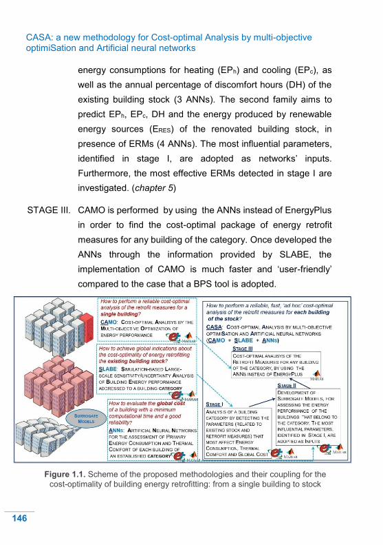
CASA: a new methodology for Cost-optimal Analysis by multi-objective optimiSation and Artificial neural networks
146
energy consumptions for heating (EPh) and cooling (EPc), as
well as the annual percentage of discomfort hours (DH) of the
existing building stock (3 ANNs). The second family aims to
predict EPh, EPc, DH and the energy produced by renewable
energy sources (ERES) of the renovated building stock, in
presence of ERMs (4 ANNs). The most influential parameters,
identified in stage I, are adopted as networks’ inputs.
Furthermore, the most effective ERMs detected in stage I are
investigated. (chapter 5)
STAGE III. CAMO is performed by using the ANNs instead of EnergyPlus
in order to find the cost-optimal package of energy retrofit
measures for any building of the category. Once developed the
ANNs through the information provided by SLABE, the
implementation of CAMO is much faster and ‘user-friendly’
compared to the case that a BPS tool is adopted.
Figure 1.1. Scheme of the proposed methodologies and their coupling for the
cost-optimality of building energy retrofitting: from a single building to stock

CASA: a new methodology for Cost-optimal Analysis by multi-objective optimiSation and Artificial neural networks
147
6.3. Application
6.3.1. Presentation of the case study
CASA is applied for assessing the cost-optimal energy retrofitting strategy
of a building belonging to the category investigated by means of SLABE
and ANNs, namely: Office buildings built in South Italy in the period 1920-
1970. More in detail, the methodology is implemented to the reference
building (RefB) related to such category, detailed in section 4.3.1.
Therefore, the first two stages of CASA have been already applied in the
previous part of this thesis. Indeed, SLABE has been performed to the
considered category in chapter 4, and the ANNs related to the examined
buildings have been developed in chapter 5, by exploiting the data
provided by SLABE. In the following lines, the application of the final stage
of CASA is carefully described and the cost-optimality is assessed.
In particular, CAMO is applied to the building, by using the ANNs instead
of EnergyPlus, in order to investigate the following ERMs:
installation of a new external coating of the roof, characterized by a
low solar absorptance (a);
installation of external thermal insulation of the roof;
installation of external thermal insulation of the vertical envelope;
installation of a mechanical ventilation system, for achieving free
cooling when the outdoor temperature is lower than the indoor one in
summertime;
variation of the set points of indoor temperature, during both heating
and cooling seasons;
replacement of the single-glazed windows with low-emissive double-
glazed ones;
replacement of the present standard boiler with a condensing one
(η=1.06);

CASA: a new methodology for Cost-optimal Analysis by multi-objective optimiSation and Artificial neural networks
148
replacement of the air-cooled chiller with a water-cooled one
(EER=4.5), with the consequent installation of a cooling tower;
installation of polycrystalline PV panels on the roof.
These ERMs have been selected on the basis of the outcomes provided
by SLABE for the considered category. Indeed, they are the most
affecting the building energy and thermal behavior. For a detailed
description of such retrofit measures, the readers are invited to refer to
section 4.3.1. Of course, only these measures have been considered in
the generation of the four ANNs related to the renovated building stock.
Eventually, the following design variables (the number is of the order of
10, as recommended by Wetter [95]) can be identified:
absorption coefficient of solar radiation of the roof (a);
thickness of the insulation of roof (tr);
thickness of the insulation of vertical walls (tv);
free cooling by means the mechanical ventilation system;
set point temperature of indoor air during the heating season (Theat);
set point temperature of indoor air during the cooling season (Tcool);
window: single/double glazed;
boiler: old standard / condensing one;
chiller: air- or water-cooled;
percentage of the roof covered by PV panels.
Each design choice can assume different discrete values, since CAMO
operates with discrete variables (see section 3.2.1). These allowable
values and the associated investment costs (IC), if present, are reported
in table 6.1, where the configuration of the reference building is also
shown. The of IC are taken from chapter 5 (see tables 4.4 and 4.5).

CASA: a new methodology for Cost-optimal Analysis by multi-objective optimiSation and Artificial neural networks
149
It is noted that, diversely from the previous application of CAMO to e
residential building (see chapter 3), also a RES system, i.e.,
photovoltaics, has been investigated, because PV panels exercise a huge
impact on the energy performance of office buildings, characterized by
high electric uses.
Table 6.1. Option values and investment cost (IC) of the design variables
DESIGN VARIABLES OPTION VALUES REFERENCE BUILDING IC [€]
a 0.05 4320 0.50 ● - 0.95 4320
tr
0 cm ● - 3 cm 4059 6 cm 6336 9 cm 6783
tv
0 cm ● - 3 cm 5495 6 cm 8578 9 cm 9182
free cooling no ● - Yes 7610
Theat
19°C - 20 °C ● - 21 °C - 22 °C -
Tcool
24 °C - 25 °C - 26 °C ● - 27 °C -
window type
single glazed (Uw = 5.8 W/m2K)
● -
double glazed low-e (Uw = 1.9 W/m2K)
21600
boiler type old ● - condensing 8100
chiller type air-cooled ● - water-cooled 21500
PV: roof coverage 0 – 100% with a step of 10%
0% 3 €/Wp

CASA: a new methodology for Cost-optimal Analysis by multi-objective optimiSation and Artificial neural networks
150
CAMO is applied to the delineated case study, in conjunction with ANNs,
by adopting the parameters of the GA reported in table 6.2. The GA
performs the multi-objective optimization of primary energy consumption
per unit of conditioned area (PEC’) and annual percentage of discomfort
hours (DH), in presence of the aforementioned design variables that
represent ERMs. PEC’ and DH are evaluated by means of the second
family of ANNs, developed for investigating the ERMs (see chapter 5). It
is noted that PEC’ is preferred, as objective, to the primary energy
demand for space conditioning (EP), used in the previous application of
CAMO, in order to contemplate the benefits induced by the PV panels.
Table 6.2. Setting of the control parameters (see section 3.2.2) of the GA
s ce fc fm gmax tol
50 2 0.6 0.1 200 0.001
The values of the population size (s) and of the maximum number of
simulations (gmax) is quite higher compared to the application of CAMO
proposed in chapter 3. Indeed, the adoption of ANNs (50 vs 25 for s, 200
vs 30 for gmax), instead of EnergyPlus simulations, allows to save around
98% of the computational time for energy simulations, as argued in the
previous chapter. Therefore, the implementation of the networks in
CAMO yields a double benefit, because it ensures a more reliable Pareto
front in a time much lower.
It is also worthy to note that the number of energy simulations, required
for investigating all possible retrofit strategies, would be 122880, while
the optimization procedure takes a maximum of 10000 simulations. Thus,
an exhaustive analysis carried out by means of EnergyPlus would involve
a computational time around 70 days, while the adoption of CAMO
coupled with ANNs (inside CASA) would imply a computational time lower
than 3 hours. It’s clear that the capability of CASA is enormous.

CASA: a new methodology for Cost-optimal Analysis by multi-objective optimiSation and Artificial neural networks
151
6.3.2. Results and discussion
It is recalled that the first phase of CAMO involves the multi-objective
optimization of PEC’ and DH, in correspondence of different available
economic budgets. In this case study, since the maximum total
investment cost of the retrofit actions is 120000 €, the optimization
procedure has been performed for the following four budgets: 30000 €,
60000 €, 90000 €, 120000 € (corresponding to an unlimited availability).
The Pareto fronts achieved for these four budgets are depicted in figure
6.1, where the ‘best’ solution, with reference to each budget and using
the minimum comfort criterion (DHmax = 20%), is highlighted by means of
a bigger black marker. The values assumed by the design variables in
correspondence of these best packages and the relative investment costs
are listed in table 6.3, where the packages are respectively indicated with
the symbols P1, P2, P3, P4, (from the lowest to the highest budget).
Figure 6.1. Pareto fronts for the four budgets: the recommended packages
using the comfort criterion are highlighted through bigger black markers

CASA: a new methodology for Cost-optimal Analysis by multi-objective optimiSation and Artificial neural networks
152
Table 6.3. Design variables and investments costs (IC) of the recommended
packages
Unlike in the first application of CAMO (chapter 3), only the method of the
minimum acceptable thermal comfort is here used for the multi-criteria
decision making (MCDM), since this criterion is more relevant to the study
of building energy performance. Furthermore, the outcomes of chapter 3
has shown that the comfort method and the utopia point method lead to
similar results. The maximum acceptable value of percentage discomfort
hours (DHmax) is set at 20%. A higher threshold value has been chosen,
compared the previous application to a residential building (DHmax =
10%), because this case studies is globally characterized by higher
values of DH, as clear in the comparison between figure 6.1 and figure
3.7. This is mainly due to the high internal heat gains that penalize the
comfort in summer time. Really, depending on the occupants’ needs, the
methodology here proposed allows the choice of the most proper DHmax.
Most solutions on the Pareto fronts determine a significant improvement
compared to the reference building, whose performance is indicated in
figure 6.1 by a red cross. This underlines that the behavior of the present
BUDGETS PACKAGES 30 k€ 60 k€ 90 k€ 130 k€
P1 P2 P3 P4
a 0.5 0.5 0.5 0.05 tr 0 cm 0 cm 9 cm 9 cm tv 0 cm 3 cm 9 cm 9 cm
free cooling yes no yes yes solar shading no no yes yes
Theat 21 °C 20 °C 20 °C 20 °C Tcool 25 °C 24 °C 26 °C 25 °C
windows single glazed single glazed single glazed low-e
double glazed
boiler condensing old old condensing
chiller air-cooled water-cooled water-cooled water-cooled
PV coverage 40% 80% 100% 100% IC 28020 € 58195 € 86346 € 120000€

CASA: a new methodology for Cost-optimal Analysis by multi-objective optimiSation and Artificial neural networks
153
building is unacceptable from both the point of views of energy
consumption and thermal comfort. All told, figure 6.1 and table 6.3 yield
to original and relevant remarks, founded on physical considerations.
As the budgets increase, the fronts obviously move left without
overlapping, thereby providing a first verification of CASA reliability.
The recommended packages of ERMs for the four budgets (P1, P2, P3,
P4), summarized in table 6.3, do not include a retrofit measure that is
always present, except for PV panels. This shows that the considered
ERMs are quite interactive as argued in the following lines. As said, the
photovoltaic technology is always present because it ensures a huge
PEC’ saving. However, when the budget is quite limited (see P1 and P2)
the maximum size of PV panels compatible with the economic limit is not
implemented. Indeed, when the size increases, the energy benefit
induced by photovoltaics grows more slowly (see figure 4.14). Thus, other
ERMs are preferred to the adoption of a higher number of PV panels, in
order to improve also the second objective, that is DH, which is not
affected by photovoltaics. Besides the installation of PV panels, each of
the recommended solutions includes a mix of ERMs that aims to ensure
a trade-off between the needs of wintertime and summertime.
P1 is characterized by the presence of free cooling and condensing
boiler. This latter is preferred to the water-cooled chiller that would be
more influential on PEC’ by virtue of the magnitude of cooling demand
(see figure 4.11). This could appear strange but, actually, it is a proof of
the reliability of the methodology because the choice of replacing the
chiller, instead of the boiler, would be more expensive, thereby reducing
the size of photovoltaics and avoiding the adoption of ERMs for the other
(heating) season. Diversely, P1 provides a more balanced and effective
mix of measures directed to all the energy uses of the building, i.e.,
heating, cooling and electricity. Moreover, it includes more comfortable

CASA: a new methodology for Cost-optimal Analysis by multi-objective optimiSation and Artificial neural networks
154
set point temperatures in both season compared to the reference
building, while nevertheless ensuring a lower PEC’.
P2 provides a higher size of photovoltaics, albeit still lower than the
maximum one, as well as a 3 cm thick insulation of the vertical walls and
the water-cooled chiller. In this case, the replacement of the chiller is
preferred to that of the boiler, because the higher budget allows the
implementation of the insulation, which produces a reduction of heating
demand and DH. Indeed the value of DH is significantly influenced by the
levels of thermal comfort during winter and intermediate seasons
(summer covers a small period), which benefit from the presence of an
insulated building envelope because of higher values of the mean radiant
temperature. Consequently, an increment of this parameter allows a
reduction of Theat compared to P1 (20°C vs 21°C), which obviously is
convenient from the energy and economic points of view. Diversely, the
thermal comfort in summertime is penalized, by requiring a reduction of
Tcool compared to P1 (24°C vs 25°C), not convenient from the
aforementioned points of view. All told, also this package of measures
contemplates all the energy uses of the building.
P3 implements all the considered ERMs, except for the low-a plastering
of the roof, the low-e windows and the condensing boiler. PV panels cover
the whole roof surface; so the maximum power is installed. Both roof and
vertical walls are insulated, by adopting the maximum insulant thickness,
i.e., 9 cm. This determines a strong reduction of energy demand for
heating and a substantial improvement of thermal comfort during winter
and intermediate seasons. On the other hand, the implementation of free
cooling and external solar shading yields substantial benefits on cooling
demand and thermal comfort in summertime. Thus, the ERMs are
balanced and provide an optimal trade-off among the different building

CASA: a new methodology for Cost-optimal Analysis by multi-objective optimiSation and Artificial neural networks
155
need. In fact, there isn’ t the necessity of modifying the set point
temperatures compared to the reference building.
P4 implements all the investigated ERMs. This is possible by virtue of an
unlimited available budget. In general, this result is not obvious (for
instance, see the previous application of CAMO) but, in this case, it was
expected because the ERMs have been properly chosen by means of
SLABE. The main differences between P4 and P3 consist in the presence
of the low-a roof plastering, low-e windows and condensing boiler. These
measures have different effects. Indeed, the low-a plastering is beneficial
for energy demand and thermal comfort in the cooling season, while the
opposite occurs for the heating season. The condensing boiler, obviously,
determines a reduction of energy demand for heating. Eventually, the
installation of new windows with double and low-emissive glasses
induces lower thermal losses in wintertime, whereas contrasting effects
occur in summertime. Indeed, the new glazed systems reduce the
entering solar radiation, although also the favorable thermal losses from
the indoor environment to the external one, in some hours (mainly in the
intermediate seasons), are lowered. Finally, also P4 collects a balanced
mix of retrofit measures. However globally, compared to P3, such mix
slightly penalizes the thermal comfort in summertime, thereby requiring a
lower Tcool (25°C vs 26°C).
It’s quite difficult to draw up a ranking of the retrofit energy measures
based on the intervention priority as done in section 3.3.2 because of the
high synergy among them. However, it is noted that the low-a plastering
of the roof and the installation of low-e windows are implemented only if
an unlimited budget is available. It means that these energy efficiency
measures have the lowest priority, because their impact on the objectives
is less positive compared to the other measures. On the other hand, the
installation of PV panels, the achievement of free cooling by means of

CASA: a new methodology for Cost-optimal Analysis by multi-objective optimiSation and Artificial neural networks
156
mechanical ventilation and the implementation of efficient HVAC systems
represent the ERMs with the highest priority. Concerning the HVAC
system, in absence of an insulated building envelope, the priority belongs
to the replacement of the boiler with a condensing one, otherwise it
belongs to the replacement of the air-cooled chiller with a water-cooled
one. The thermal insulation of both vertical walls and roof represents a
further effective retrofit measure. Indeed, in most cases when the budget
is sufficient, the maximum thicknesses are implemented. This outcome
seems to be partially in disagreement with the results of the sensitivity
analysis performed by means of SLABE (see figure 4.9). Indeed, the
standardized rank regression coefficients (SRRCs) show that the
insulation of both walls and roof determines a significant improvement of
DH, while they exercise a slight influence on the demand of thermal
energy for space conditioning because of the contrasting effects
occurring in wintertime and summertime (see section 2.2.3. for a detailed
description). Actually, the disagreement does not subsist. In fact, in
CASA’s outcomes the presence of the thermal insulation is always
coupled with the adoption of the efficient water-cooled chiller, which
reduces the impact of energy demand for cooling on PEC’, thereby
making the insulation effective. Furthermore, CASA tends to pick this
retrofit measure because it exercise a huge positive impact on DH,
whereas PEC’ can be ‘adjusted’ by means of photovoltaics.
As done in chapter 3, after the optimization study in matter of energy
performance and thermal comfort, an economic analysis is performed for
detecting the cost-optimal package and thus ‘the best budget’ that should
be invested. Thus, the global cost (GC) is calculated for the packages
listed in table 6.3 and for the reference building. It is noticed that in
chapter 3, two cases have been investigated, namely the absence of

CASA: a new methodology for Cost-optimal Analysis by multi-objective optimiSation and Artificial neural networks
157
state incentives and the presence of a hypothetical capital grant that
covers the 50% of the investment cost (IC) for ERMs. Here, in order to
realize an evaluation closer to reality, only the presence of current
incentives provided by the Italian Government is considered. They consist
of a capital grant, according in ten years, that cover the 50% of IC for PV
panels and the 65% of IC for condensing boiler, efficient windows and
thermal insulation that allows to fulfill the U values prescribed by the law
(in this case, for both walls and roof, the incentive is accorded only in
presence of a 9 cm thick insulant). These incentives are not contemplated
during the optimization procedure for assessing IC related the ERMs
packages, which should fulfill the economic budget, because they are
differed in ten years and so they are not perceived by the users as an
actual reduction of the initial disbursement, for which the constraint is
conceived. For GC evaluation, a calculation period of 20 years is used,
as prescribed by the guidelines of the EPBD Recast for non-residential
buildings. The prices of electricity and natural gas, and primary energy
factors assume the values shown in section 4.3.2.
The values of DH, PEC’ and GC – which are the main objectives of this
study – in correspondence of P1, P2, P3, P4 and RefB are shown in table
6.4, where the results achieved by means of ANNs are compared to those
provided by EnergPlus in order to further verify the reliability of CASA.
The percentage relative error committed by the newtorks is reported for
each of the mentioned objectives. Finally, the values of GC for the four
recommended packages (P1, P2, P3, P4) and the RefB are depicted in
figure 6.2, where the cost-optimal package of ERMs is highlighted. In this
figure, the solutions are put in order of increasing PEC’, for recalling the
typical cost-optimal curve (see figure 2.3) where the point of minimum
represents the cost-optimality.

CASA: a new methodology for Cost-optimal Analysis by multi-objective optimiSation and Artificial neural networks
158
Table 6.4. Values of objective functions and global cost for recommended
packages and reference building: comparison between ANNs and EnergyPlus
*Cost-optimal solution
Figure 6.2. Global cost of the recommended packages in presence of Current
Incentives and cost-optimal solution
BUDGETS REFERENCE BUILDING
PACKAGES 30 k€ 60 k€ 90 k€ 130 k€
P1 P2 P3 P4
AN
NS PEC’ [kWh/ m2 a] 211.5 162.0 134.8 123.4 239.1
DH [%] 17.5 17.8 19.0 18.1 33.6
GC [€] 148615 140180 133130* 137260 152720
EN
ER
GY
PLU
S
PEC’ [kWh/ m2 a] 212.5 164.3 134.5 124.4 238.5
DH [%] 19.0 21.8 23.6 22.0 35.5
GC [€] 149320 140470 131750* 135900 152320
ER
RO
R
OF
AN
NS
PEC’ -0.5% -1.4% 0.2% -0.8% 0.3%
DH -8.6% -22.0% -24.0% -22.0% -5.7%
GC -0.5% -0.2% 1.0% 1.0%
0.6%

CASA: a new methodology for Cost-optimal Analysis by multi-objective optimiSation and Artificial neural networks
159
Table 6.4 shows that the results provided by ANNs are very reliable as
for PEC’ and GC predictions, since the maximum absolute relative error
related to EnergyPlus simulations is respectively equal to 1.4% for PEC’
and 1% for GC. On the other hand, the network for the assessment of
DH is less accurate, as already noticed in section 5.3.2, because thermal
comfort is ruled by more complicated phenomena, which are hardly
predictable. The maximum absolute relative error is equal to 24%
However, such ANN is able to predict the trend of DH. Indeed, both the
network and EnergyPlus outputs determine that DHRefB>DHP3> DHP4>
DHP3> DHP1. This is the most important feature concerning thermal
comfort that the network must own in order to achieve a faithful
comparison between different ERMs packages. Indeed, the calculation of
the precise value of DH is quite aleatory and also the number given by
EnergyPlus is not completely credible. That’s why, the main thing is the
capability of predicting the increasing or decreasing trend of DH.
Therefore, also the performance of the ANN for DH assessment is
considered satisfying.
The cost-optimal package is represented by P3, and thus the ‘cost-
optimal’ budget to invest is equal to 90000 €. This yields a GC saving of
around 19600 € in the building life-cycle, compared to the reference
building.
This output differs from the cost-optimal package identified by means of
SLABE for most buildings of the category (see figure 4.16) because
CASA gives a greater importance to thermal comfort, which is an
objective whereas in SLABE it is a secondary criterion for selecting
ERMs. Therefore, the cost-optimal solution by CASA includes the thermal
insulation of roof and external walls, while that by SLABE doesn’t. On the
other hand, the two cost-optimal packages present the same HVAC
system and size of PV panels.

CASA: a new methodology for Cost-optimal Analysis by multi-objective optimiSation and Artificial neural networks
160
Finally, CASA can be applied to any building for detecting the cost-
optimal package of energy retrofit measures by means of a reliable, fast,
‘ad hoc’ procedure. This induces both a saving of global cost, thus of
money, and a reduction of energy consumption, thus polluting emissions,
of the building sector.
Therefore, a double ‘optimum’ is achieved: an economic ‘optimum’ for the
buildings’ owners/ occupants; an environmental ‘optimum’ for the
community.
This means multi-objective optimization.

Conclusions
161
CHAPTER 7. Conclusions
The recast version of the Energy Performance of Building Directive
(2010/31/EU) underlines the necessity of a building activity aimed at the
most proper levels of energy efficiency “with a view to achieving cost-
optimal levels”. More in detail, it prescribes the cost-optimal analysis for
detecting the best package of energy efficiency measures (EEMs) to
apply to new or existing buildings. This study is focused on the energy
retrofitting of existing constructions because it is a key-strategy to achieve
tangible results in the reduction of energy consumption, and thus polluting
emissions, of the building sector.
All told, the cost-optimal analysis is a complex and time-consuming
procedure that requires several dynamic energy simulations by building
performance simulation tools. Thus, it cannot be applied to each single
building. That’s why the EPBD Recast demands the Member States to
define a set of reference buildings (RefBs) in order to represent the
national building stock, and to perform the cost-optimal analysis only on
these representative buildings. The results achieved for each RefB about
the cost-optimal configurations of EEMs should be extended to the other
buildings of the same category, where a category is meant as a stock of
buildings, which share climatic conditions (location), functionality,
construction type. However, it’s clear that this procedure cannot ensure
reliable results for each building. Therefore, a crucial question arises:
How to perform a reliable, fast, ‘ad hoc’ cost-optimal analysis of the retrofit
measures for each building of the stock?
This thesis aims to answer this question by proposing a novel multi-stage
methodology, denominated CASA, which represents an absolute novelty
for the current scientific literature.
Conclusions
162
CASA represents the combination and ultimate fulfillment of other three
original methodologies proposed in this study, namely CAMO, SLABE
and the simulation of building energy and thermal behavior by means of
ANNs. Indeed, the acronym CASA has a double meaning. On one hand,
it reveals the combination among CAMO, SLABE and ANN. On the other
hand, it points out the core of the methodology, that is the Cost-optimal
Analysis by multi-objective optimiSation and Artificial Neural Networks.
CAMO, SLABE and ANNs can be used either as stand-alone procedures
for pursuing worthy aims or as stages of CASA for reaching the final goal
expressed by the aforementioned question.
In the following lines, the purpose and the main outcomes obtained from
the independent application of CAMO, SLABE and ANNs are first
described. Then, the framework of CASA and the final results of this study
are proposed.
CAMO is a new methodology for the Cost-optimal Analysis by Multi-
objective Optimization, which aims at the identification of the cost-optimal
package of EEMs for new or existing buildings. Since this study is focused
on energy retrofitting, only existing buildings are considered and thus the
EEMs consist of energy retrofit measures (ERMs). The methodology is
based on the multi-objective optimization of energy demand for
microclimatic control and indoor thermal comfort. The optimization
procedure is performed through the coupling of EnergyPlus and
MATLAB, in which a genetic algorithm is implemented. Various economic
budgets, available for the energy refurbishment, should be identified as
constraints regarding the investment cost. Then, for each one of these
economic availabilities, the application of the methodology allows the
definition of the Pareto front, which represents the set of ‘best’ packages
of ERMs. Among the different combinations shown on the Pareto front,

Conclusions
163
for each budget, the most suitable can be selected by using various
criteria. In the present study, both the ‘utopia point method’ and the
‘minimum comfort level method’ are used for the multi-criteria decision
making (MCDM), although the second one is more relevant to building
studies. In this way, recommended packages of ERMs – that would be
otherwise determined empirically by trial – are achieved. Then, the one
characterized by the lowest value of global cost represents the cost-
optimal solution. Finally, the methodology permits a strong support to the
cost-optimal analysis.
The proposed optimization procedure has been applied to a case study,
concerning the design of the energy retrofit of a residential building
located in Naples, Southern Italy (Mediterranean area). The outcomes
show that the most proper economic budget for the refurbishment is
300000 €. The cost-optimal package of ERMs, which complies with this
constraint, includes the thermal insulation of walls (9 cm thick insulant)
and roof (3 cm thick insulant), the installation of a water-cooled chiller and
of a condensing boiler, and the implementation of free cooling by means
of a mechanical ventilation system. This package provides the following
savings of global cost (GC), evaluated according the guidelines of the
EPBD Recast:
330000 €, without incentives and by adopting the utopia point criterion;
445000 €, with incentives equal to 50% of the investment cost and by
adopting the utopia point criterion;
310000 €, without incentives and by adopting the comfort criterion;
413000 €, with incentives equal to 50% of the investment cost and by
adopting the comfort criterion.
Furthermore, in all cases, also a substantial improvement of thermal
comfort occurs, because the annual discomfort hours (DH) are reduced

Conclusions
164
of around 25 percentage points, compared to the base configuration of
the building.
Finally, CAMO ensures the evaluation of the actual cost-optimal
solutions. Diversely, standard approaches, with packages of energy
retrofit measures chosen empirically by trial, cannot guarantee the same
accuracy and feasibility, because the entire domain of possible solutions
is not completely explored. Moreover, the method provides an effective
and flexible tool for managing the thermal comfort and for understanding
its impact on the energy demand. It is noted that CAMO can be also used
when the purpose is not the cost-optimal analysis, but the definition of
incentive policies, or the optimization of energy performance and thermal
comfort of a new or existing building in presence of a budget constraint.
Nevertheless, computational time and complexity are still too high for the
application to each single building. This represents the main limit of
CAMO. Therefore, in order to achieve global indications about the cost-
optimal energy retrofitting of a group of buildings, SLABE has been
developed.
SLABE is a new multi-stage methodology aimed to investigate the
implementation of some ERMs to buildings belonging to the same
category. It is based on uncertainty and sensitivity analyses, carried out
by means of the coupling between EnergyPlus and MATLAB. Thus, it is
denoted as Simulation-based Large-scale uncertainty/sensitivity Analysis
of Building Energy performance (SLABE). The effetcs of such ERMs on
primary energy consumption (PEC) and global cost (GC) are explored in
other to achieve two main objectives:
to detect a package of ERMs that represents the cost-optimal solution
for most buildings of the analyzed category (private perspective);

Conclusions
165
to provide the policy of state incentives for ERMs that ensures the best
ratio between energy savings and state disbursement (collective
perspective).
SLABE consists of two main stages, which are subdivided respectively in
two and three steps.
Step 1 (stage I): the existing building stock is investigated and the
most influential parameters (related to geometry, envelope and other)
on energy demand for micro-climatic control and on thermal comfort
(specifically, discomfort hours) are identified.
Step 2 (stage I): some EEMs for the reduction of energy demand
(EEMsd) are selected on the basis of the results achieved in step 1
and of the characteristics of the category; their impact on energy
demand and thermal comfort is evaluated and the most influential
measures are detected.
Step 3 (stage II): the implementation of new efficient HVAC systems
is investigated, by assessing the effect on PEC and GC; this step
detects the best policy of state incentives for HVAC systems, and it
identifies the cost-optimal HVAC configuration, when the replacement
of the HVAC system is the only implemented ERM. This cost-optimal
solution is found out respectively in presence of current and proposed
incentives.
Step 4 (stage II): the implementation of renewable energy sources
(RESs) is investigated, by assessing the effect on PEC and GC; this
step detects the best policy of state incentives for RESs and it
identifies the cost-optimal combination of HVAC system and RESs .
Step 5 (stage II): the implementation of the most influential EEMsd,
identified in step 2, is investigated, by assessing the effects on PEC
and GC; this step defines the best overall policy of state incentives for

Conclusions
166
different EEMs and it identifies the cost-optimal package of ERMs,
including HVAC system, RESs and EEMsd.
As a case study, the methodology has been applied to a specific category:
office buildings built in South Italy in the period 1920-1970. The weather
data file related to Naples is used in EnergyPlus simulations, because
this city is one of the main districts in South Italy regarding the number of
office buildings and its climatic conditions are close to average conditions
in this region. Therefore, the results obtained for Naples can be extended
to many other cities of South Italy with an acceptable approximation.
Therefore, the results obtained for Naples can be extended to many other
cities of South Italy with an acceptable approximation.
The outcomes imply the following main conclusions.
A strong dispersion of the values assumed by energy demand and
thermal comfort occurs; thus, the reference building cannot provide
reliable results for all the buildings of the category (an error higher than
100% can be committed), although the investigated category is quite
restricted.
The energy performance is mainly affected by geometry parameters
(in particular number of floors and area of each floor) and other
parameters (in particular set point temperatures), while most of the
envelope parameters are neglible. This occurs because of the
magnitude of the ventilalation load.
The most inflluential EEMsd on annual energy demand are: the low-a
plastering of the roof, the installation of double-glazed low-e windows,
the implementation of external shading of the windows, the
achievement of night free cooling by means of mechanical ventilation.
On the other hand, they are almost irrelevant to the annual value of
discomfort hours, which is mainly reduced by the thermal insulation of
the envelope. However, this latter EEMd even produces a slight

Conclusions
167
increase of energy demand, by virtue of the high relevance assumed
by the cooling season.
The package of ERMs, which represents the cost-optimal solution for
most buildings of the analyzed category, does not include EEMsd in
both cases of current and proposed incentives. More in detail, the
following cost-optimal combinations are achieved:
in presence of current incentives: maximum photovoltaic (PV)
power on the buildings’ roofs, water-cooled chiller, condensing
boiler in both cases of fan coils and radiators;
in presence of proposed incentives: maximum PV power on the
buildings’ roofs, water-cooled chiller, heat pump in presence of fan
coils and new efficient boiler in presence of radiators.
It is recalled that concerning the investigated ERMs:
current incentives provide a capital grant, accorded in ten years,
that covers:
- the 65% of the investment cost of condensing boilers, heat
pumps, new efficient windows and thermal insulation that allows
to fulfill the U values prescribed by the law;
- the 50% of the investment cost of PV panels;
proposed incentives provide a capital grant, accorded in ten years,
that covers:
- the 70% of the investment cost of heat pumps, if the building is
heated by fan coils;
- the 65% of the investment cost of new efficient boilers, if the
building is heated by radiators;
- the 40% of the investment cost of PV panels.
Proposed incentives, compared to current incentives, would induce a
similar actual value of the average saving in primary energy
consumption, dPECb (62.8 vs. 62.7 kWh/a per building), in

Conclusions
168
correspondence of a significantly lower average state disbursement,
Db (37.8 vs. 44.6 k€ per building). Thus, they would ensure a higher
state profit π, ratio between dPECb and Db (1.66 vs. 1.41 kWh/€).
The main limit of SLABE is the impossibility of obtaining detailed
indications on the cost-optimal package of ERMs for each single building,
because only global recommendations about the investigated category
are provided. However, the outcomes of the uncertainty and sensitivity
analyses performed in SLABE can be exploited for the development of
meta-models, such as artificial neural networks (ANNs).
In this study, ANNs are adopted for the assessment of primary energy
demand and thermal comfort of each building belonging to a considered
category. Two families of ANNs are generated respectively for the
existing building stock and for the renovated one in presence of ERMs.
The ANNs are generated in MATLAB environment, by using EnergyPlus
outcomes as targets for training and testing the networks. The developed
surrogate models can replace the BPS tools in the evaluation of transient
energy performance and, thus, of GC, of each building of the considered
category, both in absence and in presence of ERMs. The benefit consists
of a drastic reduction of computational burden and complexity. As
aforementioned, SLABE can provide a significant support to the
development of reliable ANNs. Indeed, SLABE allows to perform a
propaedeutic investigation of the considered building category by means
of uncertainty and sensitivity analysis. Such procedure yields the
detection of the most influential parameters on energy and thermal
behavior of the buildings, concerning both the current configuration of the
stock and the renovated one characterized by the presence of ERMs.
Thus, these parameters are used as inputs of the networks, thereby
ensuring a proper, reliable, ‘ad hoc’ development of each ANN.

Conclusions
169
The methodology is applied to the buildings that belong to the category
investigated by means of SLABE. The information gathered by means of
SLABE allowed to optimize the generation of seven ANNs, three for
defining the existing building stock and four for assessing the impact of
ERMs. More in detail, the first family of ANNs consists of three networks,
all characterized by a single output, aimed to assess respectively:
the primary energy demand for heating (ANN for EPh);
the primary energy demand for cooling (ANN for EPc );
the percentage of annual discomfort hours (ANN for DH).
The second family of ANNs consists of other four networks, related to the
renovated building stock, characterized by a single output and finalized
to assess respectively:
the primary energy demand for heating (ANN for EPh);
the primary energy demand for cooling (ANN for EPc);
the percentage of annual discomfort hours (ANN for DH);
the electricity produced by PV panels (unique RES investigated in this
case study) and consumed by the facility (ANN for EPV).
The ANNs’ energy outputs can be post-processed in MATLAB in order to
calculate the values of PEC and GC for each building of the category.
The performance of the networks are estimated by considering the
regression as well as the distributions of the relative errors between
ANN’s outputs and targets provided by EnergyPlus simulations. The
following main results about ANNs’ reliability are achieved.
For the first family of ANNs, the average relative errors are quite good,
respectively 6.1% for EPh, 6.9% for EPc and 8.4% for DH. The
regressions between the ANNs’ predictions and the simulated targets,
also show a good agreement with regression coefficients (R) very
close to 1.

Conclusions
170
The performance of the second family of ANNs for EPh, EPc and DH
is quite similar, albeit a slight worsening, to that of the first family.
Indeed, the average absolute relative errors are respectively equal to
8.0% for EPh, 8.1% for EPc and 11% for DH, as well as the regression
coefficients are lower, but still very close to one. This outcome is quite
obvious because the ANNs related to the renovated stock aim to
predict the behavior of a more complex, wide and various system. The
network for the prediction of EPV, performs very well (R = 0.997,
average absolute relative errors = 2.0%) because it is characterized
by only three inputs, consisting of building form ratio, number of floors
and percentage of the roof covered by polycrystalline PV panels.
The networks for the assessment of DH are less accurate because the
evaluation of thermal comfort is ruled by more complicated phenomena,
which are hardly predictable.
It is noticed that ANNs represent an effective tool, but they have a limit:
they are not sufficient for a robust cost-optimal analysis, since they need
to be implemented in other methodologies (e.g., CAMO), in which they
can ‘subrogate’ the traditional BPS tools.
CASA is the macro-methodology that combines CAMO, SLABE and
ANNs in order to answer the question on which this thesis is focused. It
allows to overcome the mentioned limits of CAMO, SLUSABE and ANNs,
by providing a powerful tool for a consistent, reliable and fast cost-optimal
analysis of each single building.
By referring to an established category, CASA can be subdivided in the
following three stages.
I. SLABE is implemented to explore the building category by detecting
the parameters (related to existing stock and renovated stock) and the

Conclusions
171
ERMs (renovated stock) that most affect energy performance and
thermal comfort.
II. Two families of ANNs are developed for assessing thermal comfort,
energy consumption, and thus global cost of the buildings that belong
to the category. The first family refers to existing buildings, whereas
the second one refers to renovated buildings. The most influential
parameters, identified in stage I, are adopted as Inputs and only the
most significant ERMs, also identified in stage I, are investigated.
III. CAMO is performed by using the ANNs instead of EnergyPlus in
order to find the cost-optimal package of ERMs for any building of the
category, with a low computational effort and time for the users.
As case study, CASA has been applied to a building belonging to the
same category investigated by means of SLABE and ANNs. More in
detail, the methodology is implemented to the reference building related
to such category. Only the ‘minimum comfort level method’ has been
adopted for MCDM because it is considered more relevant to building
applications. The outcomes show that the cost-optimal package of ERMs
is achieved in correspondence of the economical budget of 90000 €. It
includes the thermal insulation of walls (9 cm thick insulant) and roof (9
cm thick insulant), the installation of a water-cooled chiller, the
implementation of free cooling by means of a mechanical ventilation and
of an external solar shading system, as well as of the maximum size of
PV panels installable on building roof. The economic analysis is carried
out in presence of the aforementioned current incentives provided by the
Italian Government. The cost-optimal package of retrofit measures
produces the following main benefits compared to the reference building:
the GC over the building life-cycle is reduced of around 19600 €;
the value of DH is reduced of around 15 percentage points.

Conclusions
172
Finally, the reliability of CASA has been verified by comparing the values
of PEC, DH and GC provided by the ANNs for the recommended
packages, with those obtained by means of EnergyPlus simulations.
The results are very good for PEC and GC predictions, since the
maximum absolute relative error committed by the networks is equal
to 1.4% for PEC and 1% for GC. On the other hand, the ANN for the
assessment of DH is less accurate (maximum absolute relative error
equal to 23.6%), as expected. However, such network is able to
predict the increasing or decreasing trend of DH, therefore its
performance is considered satisfying.
In conclusion, CASA can be applied to any category, and thus to any
building for achieving a reliable, fast, ‘ad hoc’ cost-optimal analysis of the
ERMs. In other words, CASA allows each single building to know and
implement the cost-optimal package of retrofit measures. In this way, a
double benefit is reached: a benefit for the buildings’ owners/occupants,
who obtain the maximum economic saving, and a benefit for the
community/environment, because a wide diffusion of cost-optimal energy
retrofits would determine a huge reduction of energy consumption and
polluting emissions of the building sector.
This means sustainability.

Nomenclature
173
Nomenclature
A Conditioned building area m2
a, b,.., h Labels of the EEMsd ---
a Absorption coefficient of solar radiation ---
B Budget €
Bz Recommended package according to the utopia point
criterion for the budget of z00000 €
---
Bz’ Recommended package according to the comfort
criterion for the budget of z00000 €
---
COP Coefficient of performance of a heat pump WTH/WEL
c Specific heat J/kg K
ce Elite count ---
DH Percentage of annual discomfort hours %
DHmax Maximum value of DH, using the minimum comfort
level criterion
%
Db Actual value of average state disbursement per building €
d Density kg/m3
dh Annual discomfort hours h
dPECb Actual value of the average saving in primary energy
consumption per building
kWh/a
ED Annual thermal energy demand kWh/m2a
EP Annual primary energy demand kWh/m2a
EER Energy Efficiency Ratio of a chiller WTH/WEL
EPPV Electricity produced by PV panels and consumed kWh/m2a
EPRES Energy produced by RESs and consumed kWh/m2a
e Number of parameters describing the EEMsd ---
F Vector of objective functions ---
fc Crossover fraction ---
fm Mutation probability ---
GC Global cost €
gmax Maximum number of generations ---
h Annual occupied hours h
IC Initial investment cost €
k Thermal conductivity W/m K
Nomenclature
174
N Number of decision variables ---
n Number of parameters describing the existing stock ---
nb Number of budgets ---
ni Number of bits encoding the i-th decision variable ---
PEC Annual primary energy consumption kWh/a
PEC’ Annual primary energy consumption per unit of
conditioned area
kWh/m2a
p Percentage of samples(buildings) with GC savings ---
pi i-th parameter ---
R Coefficient of regression ---
RT Thermal resistance m2K/W
r Ratio between the number of samples and the number
of parameters
---
S Sampling set, collecting building instances ---
SRRC Standardized rank regression coefficient ---
s Population size ---
Theat Set point temperature during the heating season °C
Tcool Set point temperature during the cooling season °C
t Thickness m
tol Tolerance in the average change of the Pareto front ---
U Thermal Transmittance of opaque components W/m2K
Uw Thermal transmittance of the windows (glass+fame) W/m2K
x Vector of decision variables ---
Greek symbols
η Nominal efficiency of a gas boiler related to the low
calorific value
WTH/WP
μ Mean value ---
π State profit, ratio between dPECb and Db kWh/€ a
σ Standard deviation ---
Subscripts
BB Base Building
c Referred to the cooling season

Nomenclature
175
h Referred to the heating season
r Referred to the roof
v Referred to the vertical opaque walls
Acronyms
ACC Efficient air-cooled chiller
ANN Artificial neural networks
BPS Building performance simulation
CAMO Cost-optimal analysis by multi-objective optimization
CASA Cost-optimal analysis by multi-objective optimisation and artificial
neural networks (CAMO+SLABE+ANN)
CB Condensing boiler
DHW Domestic hot water
EEM Energy efficiency measure
EEMd Energy efficiency measure for the reduction of energy demand
ERM Energy retrofit measure
GA Genetic algorithm
HP Heat pump
HVAC Heating, ventilating and air conditioning
MCDM Multi-criteria decision making
MLP Feed-forward multi-layer perceptron
nZEB Nearly zero-energy buildings
PI Performance indicator
PV Photovoltaic
RB Reference boiler
RC Reference chiller
RefB Reference building
RES Renewable energy source
RMSE Root mean squared error
SA Sensitivity analysis
SLABE Simulation-based large-scale uncertainty/sensitivity analysis of
building energy performance
UA Uncertainty analysis
WCC Water-cooled chiller
References
176
References
[1] EU COM 112 (2011), A Roadmap for moving to a competitive low carbon
economy in 2050, Brussels: Communication from the Commission to the
European Parliament, the Council, the European Economic and Social
Committee and the Committee of the Regions n° 112.
[2] Odyssee (2012), Energy Efficiency Trends in Buildings in the EU, Lessons
from the ODYSSEE MURE project, <http://www.odyssee-indicators.org>.
[3] H. Khatib, IEA world energy outlook 2011: a comment, Energy Policy 48
(2012) 737-43.
[4] P. Caputo, G. Pasetti, Overcoming the inertia of building energy retrofit at
municipal level: The Italian challenge, Sustainable Cities and Society
(2015).
[5] Z. Ma, P. Cooper, D. Daly, L. Ledo, Existing building retrofits: Methodology
and state-of-the-art, Energy and Buildings 55 (2012) 889-902.
[6] C.J. Hopfe, G.L. Augenbroe, J.L. Hensen, Multi-criteria decision making
under uncertainty in building performance assessment, Building and
Environment 69 (2013) 81-90.
[7] EU Commission and Parliament, Directive 2010/31/EU of the European
Parliament and of the Council of 19 May 2010 on the energy performance
of buildings (EPBD Recast).
[8] EU Commission, Commission Delegated Regulation (EU) No 244/2012 of
16 January 2012 supplementing Directive 2010/31/EU of the European
Parliament and of the Council on the energy performance of buildings.
[9] US Department of Energy. Energy Efficiency and Renewable Energy
Office, Building Technology Program (2013), EnergyPlus 8.0.0.
<http://apps1.eere.energy.gov/buildings/energyplus/>.
[10] TRNSYS, A. (2000), Transient System Simulation Program. University of
Wisconsin.
[11] ESP-r, <http://www.esru.strath.ac.uk/Programs/ESP-r.htm>.
[12] IDA-ICE, IDA Indoor Climate and Energy,
<http://www.equa.se/ice/intro.html>.

References
177
[13] MATLAB - MATrixLABoratory (2010) - 7.10.0. User's Guide, MathWorks
[14] EU Commission and Parliament, Directive 2002/91/CE of the European
Parliament and of the Council of 16 December 2002 on the energy
performance of buildings (EPBD).
[15] EU Commission and Parliament. Directive 2012/27/EU of The European
Parliament and of the Council of 25 October 2012 on energy efficiency.
[16] IEA, <http://www.ecbcs.org/>.
[17] Decreto Legge (legislative decree), 4 Giugno 2013, n°63 [in Italian].
[18] C.H. Baek, S.H. Park, Changes in renovation policies in the era of
sustainability, Energy and Buildings 47 (2012) 485-96.
[19] L. Tobias, G. Vavaroutsos, Retrofitting Buildings to be Green and Energy-
Efficient: Optimizing Building Performance, Tenant Satisfaction, and
Financial Return. Chicago, IL, USA: Urban Land Institute, 2012.
[20] P. Hoes, J.L.M. Hensen, M.G.L.C. Loomans, B. De Vries, D. Bourgeois,
User behavior in whole building simulation, Energy and Buildings 41(3)
(2009) 295-302.
[21] J. Owens, H. Wilhite, Household energy behaviour in Nordic countries –
an unrealized energy saving potential, Energy 13 (1988) 853-59.
[22] O.G. Santin, L. Itard, H. Visscher, The effect of occupancy and building
characteristics on energy use for space and water heating in Dutch
residential stock, Energy and Buildings 41 (2009) 1223-32.
[23] V. Richalet, F.P. Neirac, F. Tellez, J. Marco, J.J. Bloem, HELP (house
energy labeling procedure): methodology and present results, Energy and
Buildings 33 (2001) 229-33.
[24] B. Poel, G.V. Cruchten, C.A. Balaras, Energy performance assessment of
existing dwellings, Energy and Buildings 39 (2007) 393-403.
[25] F. Nemry, A. Uihlein, C.M. Colodel, C. Wetzel, A. Braune, B. Wittstock, I.
Hasan, J.Kreißig, N. Gallon, S. Niemeier, Y. Frech, Options to reduce the
environmental impacts of residential buildings in the European Union –
potential and costs, Energy and Buildings 42 (2010) 976-84.

References
178
[26] S. Cohen, C. Goldman, J. Harris, Energy savings and economics of
retrofitting single-family buildings, Energy and Buildings 17 (1991) 297-
311.
[27] T. Stovall, T. Petrie, J. Kosny, P. Childs, J. Atchley, K. Sissom, An
exploration of wall retrofit best practices, in: Thermal Performance of the
Exterior Envelopes of Buildings X, Proceedings of ASHRAE THERM X,
Clearwater, FL, December, 2007.
[28] S. Nabinger, A. Persily, Impacts of airtightening retrofits on ventilation
rates and energy consumption in a manufactured home, Energy and
Buildings 43 (2011) 3059-67.
[29] H. Hens, Energy efficient retrofit of an end of the row house: confronting
predictions with long-term measurements, Energy and Buildings 42 (2010)
1939-47.
[30] C. Goodacre, S. Sharples, P. Smith, Integrating energy efficiency with the
social agenda in sustainability, Energy and Buildings 34 (2002) 53-61.
[31] P.J. Boait, D. Fan, A. Stafford, Performance and control of domestic
ground source heat pumps in retrofit installations, Energy and Buildings
43 (2011) 1968-76.
[32] K. Kuusk, T. Kalamees, M. Maivel, Cost effectiveness of energy
performance improvements in Estonian brick apartment buildings, Energy
and Buildings 77 (2014) 313-22.
[33] A. Dodoo, L. Gustavsson, R. Sathre, Life cycle primary energy implication
of retrofitting a wood-framed apartment building to passive house
standard, Resources, Conservation and Recycling 54 (2010)1152-60
[34] Y.G. Xing, N. Hewitt, P. Griffiths, Zero carbon buildings refurbishment – a
hierarchical pathway, Renewable and Sustainable Energy Reviews 15
(2011) 3229-36.
[35] E. Rey, Office building retrofitting strategies: multicriteria approach of an
architectural and technical issue, Energy and Buildings 36(4) (2004) 367-
72.

References
179
[36] C.A. Roulet, F. Flourentzou, H.H. Labben, M. Santamouris, I. Koronaki, E.
Dascalaki, V. Richalet, ORME. A multicriteria rating methodology for
buildings, Building and Environment 37 (2002) 579-86.
[37] Arup, Existing Buildings Survival Strategies: A Toolbox for Re-energising
Tired Assets, Arup and Property Council of Australia (PCA), Victorian
Division, Australia, 2008.
[38] V. Olgyay, C. Seruto, Whole-building retrofits: a gateway to climate
stabilization, ASHRAE Transactions 116 (Part 2) (2010) 244-51.
[39] C. Fluhrer, E. Maurer, A. Deshmukh, Achieving radically energy efficient
retrofits: The Empire State Building example, ASHRAE Transactions 116
(Part 2) (2010) 236.
[40] A.G. Hestnes, N.U. Kofoed, Effective retrofitting scenarios for energy
efficiency and comfort: results of the design and evaluation activities within
the OFFICE project, Building and Environment 37 (2002) 569-74.
[41] S.E. Chidiac, E.J.C. Catania, E. Morofsky, S. Foo, Effectiveness of single
and multiple energy retrofit measures on the energy consumption of office
buildings, Energy 36 (2011) 5037-52.
[42] E. Dascalaki, M. Santamouris, On the potential of retrofitting scenarios for
offices, Building and Environment 37 (2002) 557-67.
[43] A. Cooperman, J. Dieckmann, J. Brodrick, Commercial envelopes,
ASHRAE Journal 53 (2011) 134-36.
[44] D.H.C. Chow, Z. Li, J. Darkwa, The effectiveness of retrofitting existing
public buildings in face of future climate change in the hot summer cold
winter region of China, Energy and Buildings 57 (2013) 176-86.
[45] S. Barlow, D. Fiala, Occupant comfort in UK offices—how adaptive comfort
theories might influence future low energy office refurbishment
strategies, Energy and Buildings 39(7) (2007) 837-46.
[46] F. Flourentzou, J.L. Genre, C.A. Roulet, TOBUS software – an interactive
decision aid tool for building retrofit studies, Energy and Buildings 34
(2002) 193-202.

References
180
[47] Y.K. Juan, P. Gao, J. Wang, A hybrid decision support system for
sustainable office building renovation and energy performance
improvement, Energy and Buildings 42 (2010) 290-97.
[48] H. Doukas, C. Nychtis, J. Psarras, Assessing energy-saving measures in
buildings through an intelligent decision support model, Building and
Environment 44 (2009) 290-98.
[49] M. Kolokotroni, X. Ren, M. Davies, A. Mavrogianni, London’s urban heat
island: Impact on current and future energy consumption in office
buildings, Energy and Buildings 47 (2012) 302-11.
[50] D.P. Jenkins, S. Patidar, P.F.G. Banfill, G.J. Gibson, Probabilistic climate
projections with dynamic building simulation: Predicting overheating in
dwellings, Energy and Buildings 43 (2011) 1723-31.
[51] M. Santamouris, D. Kolokotsa, Passive cooling dissipation techniques for
buildings and other structures: The state of the art, Energy and Buildings
57 (2013) 74-94.
[52] M. Santamouris, D. Kolokotsa, On the impact of urban overheating and
extreme climatic conditions on housing, energy, comfort and
environmental quality of vulnerable population in Europe, Energy and
Buildings (2014).
[53] M. Santamouris, C. Cartalis, A. Synnefa, D. Kolokotsa, On the impact of
urban heat island and global warming on the power demand and electricity
consumption of buildings-A review, Energy and Buildings (2014).
[54] S.M. Porritt, P.C. Cropper, L. Shao, C.I. Goodier, Ranking of interventions
to reduce dwelling overheating during heat waves, Energy and Buildings
55 (2012) 16-27.
[55] F. Ascione, L. Bellia, P. Mazzei, F. Minichiello, Solar gain and building
envelope: The surface factor, Building Research and Information 38
(2010) 187-205.
[56] F. Ascione, N. Bianco, R.F. De Masi, F. de Rossi, G.P. Vanoli, Energy
refurbishment of existing buildings through the use of phase change
materials: Energy savings and indoor comfort in the cooling season.
Applied Energy 113 (2014) 990–1007.

References
181
[57] L. Bellia, F. De Falco, F. Minichiello, Effects of solar shading devices on
energy requirements of standalone office buildings for Italian climates,
Applied Thermal Engineering 54(1) (2013) 190-201.
[58] D. Katunský, M. Lopušniak, Impact of shading structure on energy demand
and on risk of summer overheating in a low energy building, Energy
Procedia 14 (2012) 1311-16.
[59] F. Cotana, F. Rossi, M. Filipponi, V. Coccia, A.L. Pisello, E. Bonamente,
A. Petrozzi, G. Cavalaglio, Albedo control as an effective strategy to tackle
Global Warming: A case study, Applied Energy 130 (2014) 641-47.
[60] A.L. Pisello, J.E. Taylor, X. Xu, F. Cotana, Inter-building effect: Simulating
the impact of a network of buildings on the accuracy of building energy
performance predictions, Building and Environment 58 (2012) 37-45.
[61] A.L. Pisello, V.L. Castaldo, J.E. Taylor, F. Cotana, Expanding Inter-
Building Effect modeling to examine primary energy for lighting, Energy
and Buildings 76 (2014) 513-23.
[62] S. Kamali, Review of free cooling system using phase change material for
building, Energy and Buildings 80 (2014) 131-36.
[63] C. Inard, J. Pfafferott, C. Ghiaus, Free-running temperature and potential
for free cooling by ventilation: A case study, Energy and Buildings 43(10)
(2011) 2705-11.
[64] E. Shaviv, A. Yezioro, I.G. Capeluto, Thermal mass and night ventilation
as passive cooling design strategy, Renewable Energy 24(3-4) (2001)
445-52.
[65] V. Cheng, B. Givoni, Effect of envelope color and thermal mass on indoor
temperatures in hot humid climate, Solar Energy 78 (2005) 528-34.
[66] S.P. Corgnati, E. Fabrizio, M. Filippi, V. Monetti, Reference buildings for
cost-optimal analysis: method of definition and application, Applied Energy
102 (2013) 983-93.
[67] BPIE (2013), Implementing the cost-optimal methodology in EU countries,
published in March 2013 by the Buildings Performance Institute Europe
(BPIE) <http://bpie.eu/cost_optimal_methodology.html#.UxS0s_l5OCk>.

References
182
[68] E. Pikas, M. Thalfeldt, J. Kurnitski, Cost-optimal and nearly zero energy
building solutions for office buildings, Energy and Buildings 74 (2014) 30-
42.
[69] M. Ferrara, E. Fabrizio, J. Virgone, M. Filippi, A simulation-based
optimization method for cost-optimal analysis of nearly Zero Energy
Buildings, Energy and Buildings 84 (2014) 442–57.
[70] E. Pikas, J. Kurnitski, R. Liias, M. Thalfeldt, Quantification of economic
benefits of renovation of apartment buildings as a basis for cost-optimal
2030 energy efficiency strategies, Energy and Buildings 86 (2015) 151-
160.
[71] F. Ascione, N. Bianco, C. De Stasio, G.M. Mauro, G.P. Vanoli, A new
methodology for cost-optimal analysis by means of the multi-objective
optimization of building energy performance, Energy and Buildings 88
(2015) 78-90.
[72] M. Hamdy, A. Hasan, K. Siren, A multi-stage optimization method for cost-
optimal and nearly-zero-energy building solutions in line with the EPBD-
recast 2010, Energy and Buildings 56 (2013) 189-203.
[73] A.T. Nguyen, S. Reiter, P. Rigo, A review on simulation-based optimization
methods applied to building performance analysis, Applied Energy 113
(2014) 1043-58.
[74] E. Prianto, P. Depecker, Optimization of architectural design elements in
tropical humid region with thermal comfort approach, Energy and
Buildings 35(3) (2003) 273-80.
[75] L. Wang, H. Wong Nyuk, S. Li, Facade design optimization for naturally
ventilated residential buildings in Singapore, Energy and Buildings 39(8)
(2007) 954-61.
[76] S.M. Bambrook, A.B. Sproul, D. Jacob, Design optimisation for a low
energy home in Sydney, Energy and Buildings 43(7) (2011) 1702-11.
[77] A.R. Conn, K. Scheinberg, L.N. Vicente, Introduction to derivative-free
optimization, Vol. 8. Siam, 2009.

References
183
[78] M. Hamdy, A. Hasan, K. Siren, Applying a multi-objective optimization
approach for Design of low-emission cost-effective dwellings, Building and
Environment 46(1) (2011) 109-23.
[79] M. Fesanghary, S. Asadi, Z.W. Geem, Design of low-emission and energy-
efficient residential buildings using a multi-objective optimization
algorithm, Building and Environment 49 (2012) 245-50.
[80] J.A. Wright, H.A. Loosemore, F. Farmani, Optimization of building thermal
design and control by multi-criterion genetic algorithm, Energy and
Buildings 34(9) (2002) 959-72.
[81] L. Magnier, F. Haghighat, Multiobjective optimization of building design
using TRNSYS simulations, genetic algorithm, and Artificial Neural
Network, Building and Environment 45(3) (2010) 739-46.
[82] M. Hamdy, A. Hasan, K. Siren, Impact of adaptive thermal comfort criteria
on building energy use and cooling equipment size using a multi-objective
optimization scheme, Energy and Buildings 43(9) (2011) 2055-67.
[83] B. Eisenhower, Z. O’Neill, S. Narayanan, V.A. Fonoberov, I. Mezić, A
methodology for meta-model based optimization in building energy
models, Energy and Buildings 47 (2012) 292-301.
[84] C. Diakaki, E. Grigoroudis, N. Kabelis, D. Kolokotsa, K. Kalaitzakis, G.
Stavrakakis, A multi-objective decision model for the improvement of
energy efficiency in buildings, Energy 35(12) (2010) 5483-96.
[85] F.P. Chantrelle, H. Lahmidi, W. Keilholz, M.E. Mankibi, P. Michel,
Development of a multicriteria tool for optimizing the renovation of
buildings, Applied Energy 88(4) (2011) 1386-94.
[86] <apps1.eere.energy.gov/buildings/energyplus/weatherdata_about.cfm/>.
[87] W. Tian, A review of sensitivity analysis methods in building energy
analysis, Renewable and Sustainable Energy Reviews 20 (2013) 411-19.
[88] C.J. Hopfe, J.L. Hensen, Uncertainty analysis in building performance
simulation for design support, Energy and Buildings 43(10) (2011) 2798-
805.

References
184
[89] ASHRAE, A. S. (1992). 55: Thermal environmental conditions for human
occupancy. American Society of Heating, Refrigerating and Air-
Conditioning Engineers, Atlanta.
[90] T. Hemker, K.R. Fowler, M.W. Farthing, O. von Stryk, A mixed-integer
simulation-based optimization approach with surrogate functions in water
resources management, Optimization and Engineering 9(4) (2008) 341-
60.
[91] K. Deb, Multi-objective optimization using evolutionary algorithms, Vol.
2012 John Wiley & Sons, Chichester, 2001.
[92] Y.F. Li, S.H. Ng, M. Xie, M., T.N. Goh, A systematic comparison of
metamodeling techniques for simulation optimization in decision support
systems, Applied Soft Computing 10(4) (2010) 1257-73.
[93] Y.F. Li, M. Xie, T.N. Goh,A study of project selection and feature weighting
for analogy based software cost estimation, Journal of Systems and
Software 82(2) (2009) 241-52.
[94] DesignBuilder Ltd. DesignBuilder software, Version 3.4.
[95] M. Wetter, GenOpt, a generic optimization program, Version 3.0. 0 User
Manual 3.0. 0, Technical Report LBNL-2077E, Berkeley, 2009.
[96] I. Ballarini, S.P. Corgnati, V. Corrado, Use of reference buildings to assess
the energy saving potentials of the residential building stock: The
experience of TABULA project, Energy Policy 68 (2014) 273-84.
[97] G.V. Fracastoro, M. Serraino, A methodology for assessing the energy
performance of large scale building stocks and possible applications,
Energy and Buildings 43(4) (2011) 844-52.
[98] C.A. Balaras, K. Droutsa, E. Dascalaki, S. Kontoyiannidis, Heating energy
consumption and resulting environmental impact of European apartment
buildings, Energy and Buildings 37(5) (2005) 429-42.
[99] C.A. Balaras, A.G. Gaglia, E. Georgopoulou, S. Mirasgedis, Y. Sarafidis,
D.P. Lalas, European residential buildings and empirical assessment of
the Hellenic building stock, energy consumption, emissions and potential
energy savings, Building and Environment 42(3) (2007) 1298-314.

References
185
[100] E.G. Dascalaki, K. Droutsa, A.G. Gaglia, S. Kontoyiannidis, C.A. Balaras,
Data collection and analysis of the building stock and its energy
performance—An example for Hellenic buildings, Energy and
Buildings 42(8) (2010) 1231-37.
[101] I. Theodoridou, A.M. Papadopoulos, M. Hegger, Statistical analysis of the
Greek residential building stock, Energy and Buildings, 43(9) (2011) 2422-
28.
[102] S. de Wit S, G. Augenbroe, Analysis of uncertainty in building design
evaluations and its implications, Energy and Buildings 34 (2002) 951-58
[103] Eisenhower, B., O'Neill, Z., Fonoberov, V. A., & Mezić, I. (2012).
Uncertainty and sensitivity decomposition of building energy
models. Journal of Building Performance Simulation, 5(3), 171-184.
[104] J.S Hygh, J.F. De Carolis, D.B. Hill, S. Ranji Ranjithan, Multivariate
regression as an energy assessment tool in early building design, Building
and Environment 57 (2012) 165-75.
[105] M. Wetter, J.A. Wright, A comparison of deterministic and probabilistic
optimization algorithms for non smooth simulation-based optimization,
Building and Environment 39 (2004) 989-99.
[106] M. Wetter, E. Polak, A convergent optimization method using pattern
search algorithms with adaptive precision simulation, Build Serv Eng Res
Technol 25(4) (2004) 327-38.
[107] P. de Wilde, W. Tian, Identification of key factors for uncertainty in the
prediction of the thermal performance of an office building under climate
change, Building Simulation 2 (2009) 157-74.
[108] Y. Yildiz, K. Korkmaz, T. Göksal Özbalta, Z. Durmus Arsan, An approach
for developing sensitive design parameter guidelines to reduce the energy
requirements of low-rise apartment buildings, Applied Energy 93 (2012)
337-47.
[109] J.C. Helton, J.D. Johnson, C. Sallaberry, C.B. Storlie, Survey of sampling-
based methods for uncertainty and sensitivity analysis, Reliability
Engineering & System Safety 91 (2006) 1175-209.

References
186
[110] R. Jin, W. Chen, T.W. Simpson, Comparative studies of metamodelling
techniques under multiple modelling criteria, Structural and
Multidisciplinary Optimization 23(1) (2001) 1-13.
[111] P. de Wilde, W. Tian, Predicting the performance of an office under climate
change: a study of metrics, sensitivity and zonal resolution, Energy and
Buildings 42 (2010) 1674-84.
[112] W. Tian, R. Choudhary, A probabilistic energy model for non-domestic
building sectors applied to analysis of school buildings in greater London,
Energy and Buildings 54 (2012) 1-11.
[113] M. Citterio, Analisi statistica sul parco edilizio non residenziale e sviluppo
di modelli di calcolo semplificati [Statistical analysis on the non-residential
building stock and development of simplified calculation tools], Report
RSE/2009/161, ENEA, Cresme Ricerche Spa e Ministero dello Sviluppo
Economico (2009) [in Italian].
[114] European Commission (EC), Energy Technologies, Knowledge,
Perception, Measures (Eurobarometer) 2006.
[115] PV-GIS Software, European Commission, Joint Research Centre, Institute
for Environment and Sustainability, Renewable Energies Unit, web
site: <http://re.jrc.cec.eu.int/pvgis/pv/>.
[116] <http://www.energy.eu/>.
[117] J.P.C. Kleijnen, Statistical Tools for Simulation Practitioners, Marcel
Dekker, New York, 1987.
[118] C.J. Hopfe, M.T. Emmerich, R. Marijt, J.L. Hensen, Robust multi-criteria
design optimisation in building design, In Proceedings of the building
simulation and optimization conference, Loughborough, UK (2012).
[119] E. Tresidder, Y. Zhang, A.I. Forrester, Acceleration of building design
optimisation through the use of kriging surrogate models, In: Proceedings
of the building simulation and optimization conference, September 2012.
[120] A.P. Melo, D. Cóstola, R. Lamberts, J.L. Hensen, Development of
surrogate models using artificial neural network for building shell energy
labeling, Energy Policy 69 (2014) 457-66.

References
187
[121] C.J. Hopfe, M.T. Emmerich, R. Marijt, J.L. Hensen, Robust multi-criteria
design optimisation in building design, In Proceedings of the building
simulation and optimization conference, Loughborough, UK (2012).
[122] L. Magnier, F. Haghighat, Multiobjective optimization of building design
using TRNSYS simulations, genetic algorithm, and Artificial Neural
Network, Building and Environment 45(3) (2010) 739-46.
[123] B. Dong, C. Cao, S. Lee, Applying Support Vector Machines to predict
building energy consumption in tropical region, Energy and Buildings 37
(2005) 545–53
[124] M. Brown, C. Barrington-Leigh, C., Z. Brown, Kernel regression for real-
time building energy analysis. Journal of Building Performance Simulation,
5(4) (2012) 263-76.
[125] S.A. Kalogirou, Applications of artificial neural-networks for energy
systems, Applied Energy 67(1) (2000) 17-35.
[126] G. Mihalakakou, M. Santamouris, A. Tsangrassoulis, On the energy
consumption in residential buildings, Energy and Buildings 34(7) (2002)
727-36.
[127] P.A. Gonzalez, J.M. Zamarreno, Prediction of hourly energy consumption
in buildings based on feedback artificial neural network, Energy and
Buildings 37 (2005) 595–601.
[128] S. Karatasou, M. Santamouris, V. Geros, Modeling and predicting
building's energy use with artificial neural networks: methods and results,
Energy and Buildings 38(8) (2006) 949-58.
[129] B.B. Ekici, U.T. Aksoy, Prediction of building energy consumption by using
arti-ficial neural network, Advances in Engineering Software 40 (2009)
356-62.
[130] P. Popescu, F. Ungureanu, A. Hernàndez-Guerrero, Simulation models for
the analysis of space heat consumption of buildings, Energy 34 (2009)
1447-53..
[131] O.A. Dombayci, The prediction of heating energy consumption in a model
house using artificial neural networks in Denizli-Turkey, Advances in
Engineering Software 41 (2010) 141-47.

References
188
[132] R. Mena, F. Rodríguez, M. Castilla, M.R. Arahal, A prediction model based
on neural networks for the energy consumption of a bioclimatic
building, Energy and Buildings 82 (2014) 142-55.
[133] S. Paudel, M. Elmtiri, W.L. Kling, O. Le Corre, B. Lacarriere, Pseudo
dynamic transitional modeling of building heating energy demand using
artificial neural network, Energy and Buildings 70 (2014) 81-93.
[134] S. Kalogirou, G. Florides, C. Neocleous, C. Schizas, Estimation of daily
heatingand cooling loads using artificial neural networks, in: 2001 World
Congress,Napoli, September 2001,
<http://ktisis.cut.ac.cy/bitstream/10488/883/1/C41-CLIMA2001.pdf>.
[135] A.H. Neto, F.A.S. Fiorelli, Comparison between detailed model simulation
andartificial neural network for forecasting building energy consumption,
Energyand Buildings 40 (2008) 2169–76.
[136] S.A. Kalogirou, M. Bojic, Artificial Neural Networks for the prediction of the
energy consumption of a passive solar building, Energy 25 (2000) 479-91.
[137] E. Asadi, M.G. da Silva, C.H. Antunes, L. Dias, L. Glicksman, Multi-
objective optimization for building retrofit: A model using genetic algorithm
and artificial neural network and an application, Energy and Buildings 81
(2014) 444-56.
[138] P.M. Ferreira, A.E. Ruano, S. Silva, E.Z.E. Conceicao, Neural networks
based predictive control for thermal comfort and energy savings in public
buildings, Energy and Buildings 55 (2012) 238-51.
[139] A.P. Melo, D. Cóstola, R. Lamberts, J.L. Hensen, Development of
surrogate models using artificial neural network for building shell energy
labeling, Energy Policy 69 (2014) 457-66.
[140] C. Buratti, M. Barbanera, D. Palladino, An original tool for checking energy
performance and certification of buildings by means of Artificial Neural
Networks, Applied Energy 120 (2014) 125-32.
[141] Y.F. Li, S.H. Ng, M. Xie, T.N. Goh, A systematic comparison of
metamodeling techniques for simulation optimization in decision support
systems, Applied Soft Computing 10(4) (2010) 1257-73.

References
189
[142] W.S. McCulloch, W. Pitts W, A Logical Calculus of the Ideas Immanent in
Nervous Activity, Bulletin of Mathematical Biophysics 9 (1943) 127-47.
[143] J. Conraud, A methodology for the optimization of building energy,
thermal, and visual performance, Master thesis. Canada: Concordia
University (Canada), 2008.
[144] F. Boithias, M. El Mankibi, P. Michel, Genetic algorithms based
optimization of artificial neural network architecture for buildings’ indoor
discomfort and energy consumption prediction, Building Simulation 5
(2012) 95-106, Tsinghua Press.