Multi-objective optimization of structures topology by genetic algorithms

Multi-objective optimization of structures topology by genetic algorithms

J.F. Aguilar Madeiraa,b,*, H. Rodriguesa, Heitor Pinaa

aIDMEC/IST-Mechanical Engineering Department, Instituto Superior Tecnico, Av. Rovisco Pais, 1049-001 Lisbon, PortugalbISEL-Instituto Superior de Engenharia de Lisboa, Lisbon, Portugal

Received 1 November 2002; accepted 25 July 2003

Available online 24 July 2004

Abstract

This work develops a computational model for topology optimization of linear elastic structures for situations where more than one

objective function is required, each one of them with a different optimal solution.

The method is thus developed for multi-objective optimization problems and is based on Genetic Algorithms. Its purpose is to evolve an

evenly distributed group of solutions (population) to obtain the optimum Pareto set for the given problem.

To reduce computational effort, optimal solutions of each of the single-objective problems are introduced in the initial population.

Two numerical examples are presented and discussed to assess the method.

q 2004 Civil-Comp Ltd and Elsevier Ltd. All rights reserved.

Keywords: Structural topology design; Multi-Objective Optimization; Genetic Algorithm; Evolutionary Algorithms

1. Introduction

In its most general form, the topology optimization

problem of structures can be viewed as the process of

constructing the characteristic (indicator) function of the

domain occupied by the material, i.e.

x ¼1 if material exists

0 if material doesn0t exist

(

for a given total amount of material.

The binary chromosome design and global search

capabilities of the Genetic Algorithm (GA) make is a

powerful tool for solving topology design problem [1,9].

In this work a GA for multi-objective topology

optimization of linear elastic structures, with an equality

constraint on volume, is developed. Due to this constraint all

the chromosomes used in the GA are constructed to ensure

the same volume for all individuals (designs), hence all

of them have the same number of ones (implicitly, the same

number of zeros) along the evolutionary process.

For a typical chromosome defined by L genes there are a

total of 2L possible solutions in the representation scheme.

Considering the volume equality constraint, a significant

decrease of this value can be achieved. If a chromosome

with a total of L genes is considered and K genes being one

ð1 , K , L; ðL 2 KÞ genes being zero), only

CLK ¼

L!

K!ðL 2 KÞ!

possible configurations are possible. The present analysis

explores this fact to reduce the computational effort

required. It is thus necessary to define these chromosomes

and to create accordingly new operators of crossover and

mutation that preserve this constraint.

In contrast to single-objective optimization, where

objective and fitness functions are often identical, both

fitness assignment and selection must allow for several

objectives when multi-objective optimization problems are

considered. Hence, instead of a single optima, multi-

objective optimization problems solutions consist often of

a family of points, known as the Pareto optimal set, where

each objective component of any point along the Pareto-front

can only be improved by degrading at least one of its other

objective components. In the total absence of information

regarding the preferences of objectives, a ranking scheme

based upon the Pareto optimality is regarded as an

appropriate approach to represent the strength of each

individual in an evolutionary algorithm for multi-objective

optimization [7,17].

Since a great diversity of solutions exist, additional

information obtained a priori from classical methods for

0965-9978/$ - see front matter q 2004 Civil-Comp Ltd and Elsevier Ltd. All rights reserved.

doi:10.1016/j.advengsoft.2003.07.001

Advances in Engineering Software 36 (2005) 21–28

www.elsevier.com/locate/advengsoft

* Corresponding author.

E-mail address: [email protected] (J.F.A. Madeira).

http://www.elsevier.com/locate/advengsoft

single-objective optimization is incorporated in the algo-

rithm to obtain a reduction in the computational effort.

Some mathematical support for this is given in Ref. [13].

This information is introduced in the initial population

through special individuals (see example 1 in Section 6).

2. Background

2.1. A general multi-objective optimization problem

(MOOP)

A general multi-objective optimization problem consist-

ing of k competing objectives and ðm þ p þ qÞ constraints,

defined as functions of decision variable set x; can be

represented as follows:

Minimize=Maximize fðxÞ ¼ ðf1ðxÞ; f2ðxÞ;…; fkðxÞÞ [ Y;

subject to giðxÞ # 0; ;i ¼ 1; 2;…;m;

hjðxÞ ¼ 0; ;j ¼ 1; 2;…; p;

xLl # xl # xU

l ; ;l ¼ 1; 2;…; q;

ð1Þ

where x ¼ ðx1; x2;…; xnÞ [ X:where x is the decision

vector, fðxÞ the multi-objective vector, fjðxÞ the jth objective

function, X denotes as the decision space and Y the

objective space.The constraints giðxÞ and hjðxÞ determine

the set of feasible solutions. The remaining set of constraints

are called variable bonds, restricting each decision variable

xl to values between a lower xLl and an upper xU

l bond.

2.2. Concept of domination

Most multi-objective optimization algorithms use the

concept of domination referred as Pareto optimality [14]. A

non-dominated set of solutions is formally defined as

follows [2]: ‘a feasible solution to a multi-objective problem

is non-dominated if there exists no other feasible solution

that will yield an improvement in one objective without

causing a degradation in at least one other objective’.

The set of solutions of a multi-objective optimization

problem consist then of all decision vectors which cannot be

improved in any objective without degradation in the other

objectives. This vector is know as Pareto-optima. Mathemati-

cally, the concept of Pareto-optima is as follows. Assuming,

without loss of generality, a minimization problem and

considering two decision vectors a; b [ X; we say that a

dominates b (also written as a a b) if and only if

;i[{1;2;…;k} : fiðaÞ# fiðbÞ^’j[{1;2;…;k} : fiðaÞ, fiðbÞ

ð2Þ

All decision vectors which are not dominated by any

other decision vector are called non-dominated or Pareto-

optimal. The family of all non-dominated solutions is

denoted as Pareto-optimal set (Pareto set) or Pareto-optimal

front. It is also customary to write any of the following:

† b is dominated by a;

† a is non-dominated by b; or

† a is non-inferior to b:

2.3. Multi-objective evolutionary algorithms (MOEAs)

A number of multi-objective optimization techniques

using evolutionary algorithms have been suggested since

the pioneering work by Schaffer in Refs. [15,16]. Other

important developments are described in Refs. [7].

Evolutionary optimization algorithms work with a

population of solutions instead of a single solution. Since

multi-objective optimization problems give rise to a set of

Pareto-optimal solutions, evolutionary optimization algo-

rithms are ideal for handling multi-objective optimization

problems.

In order to obtain effective results with an evolutionary

algorithm for multi-objective optimization problems we

need to guide the search toward the Pareto-optimal set and

maintain a diverse population to prevent premature

convergence and to achieve a well distributed population

in the Pareto front.

3. Methodology

As previously stated, the equality constraint on volume

requires that all chromosomes used in the GA lead to the

same volume value, hence all of them should have the same

number of ones along the evolutionary process. It is thus

necessary to properly define these chromosomes and to

create crossover and mutation operators that enforce this

volume constraint.

3.1. The chromosome storage

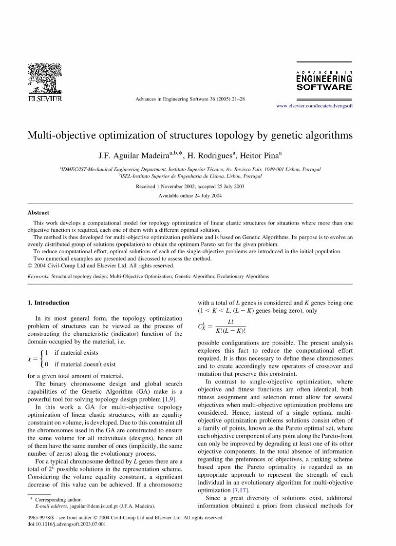
The topology model for this research is a grid that defines

the design domain. A value of 1 assigned to an element or

cell corresponds to the presence of material and a value 0 to

a void in the domain.Fig. 1 shows the structural topology

represented in the grid model (B) by the chromosome array

(C), the binary chromosome string (D) (containing the

numbering of the elements (A) and the volume value 0 or 1

for each element), and the chromosome viewed as a loop (E)

formed by joining the ends together. A chromosome

considered as a loop can represent more building blocks

for the crossover operator, since they are able to ‘wrap

around’ at the end of the string. These two last represen-

tations depend on the elements numbering.

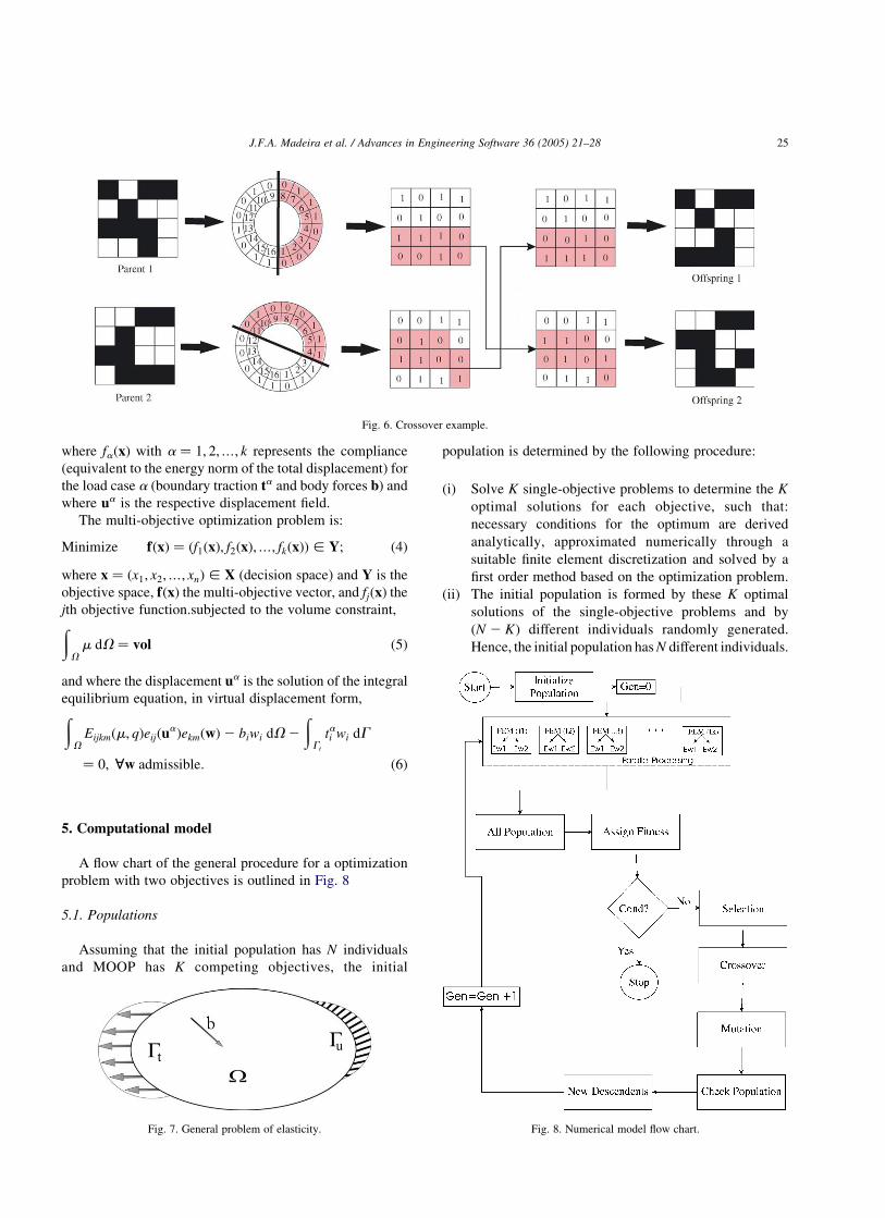
3.2. Crossover techniques

The selected progenitors exchange between them

their genetic material producing individuals with new

J.F.A. Madeira et al. / Advances in Engineering Software 36 (2005) 21–2822

characteristics. To preserve volume the progenitors and the

descendants must have the same number of ones in their

chromosomes, which requires new types of crossover to be

described below.

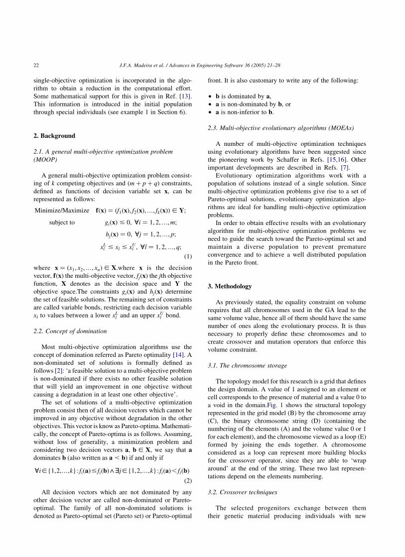
3.2.1. Algorithm

To explain these crossover techniques the chromosome’s

representation is considered as a loop (Fig. 2).

In the following crossover operator Ngc; a; p1; p2; n1s1; e

n1s2 are natural numbers representing:

Ngc Number of genes in the chromosome (in Fig. 2,

Ngc ¼ 16Þ;

a Number of genes to exchange in the crossover

operator,

p1 Number of the gene of the first progenitor where

the cut begins,

p2 Number of the gene of the second progenitor,

where the cut begins,

n1s1 Number of ones of the first progenitor existing in

the interval ½p1; p1 þ ða2 1Þ�;

n1s2 Number of ones of the second progenitor existing

in the interval ½p2; p2 þ ða2 1Þ�:

The following algorithm describes a step-by-step pro-

cedure for finding the progenitors gene sequence to use in

the crossover operator:

Step 1 Fix a; the number of genes to exchange.

Step 2 Determine the inicial p1:

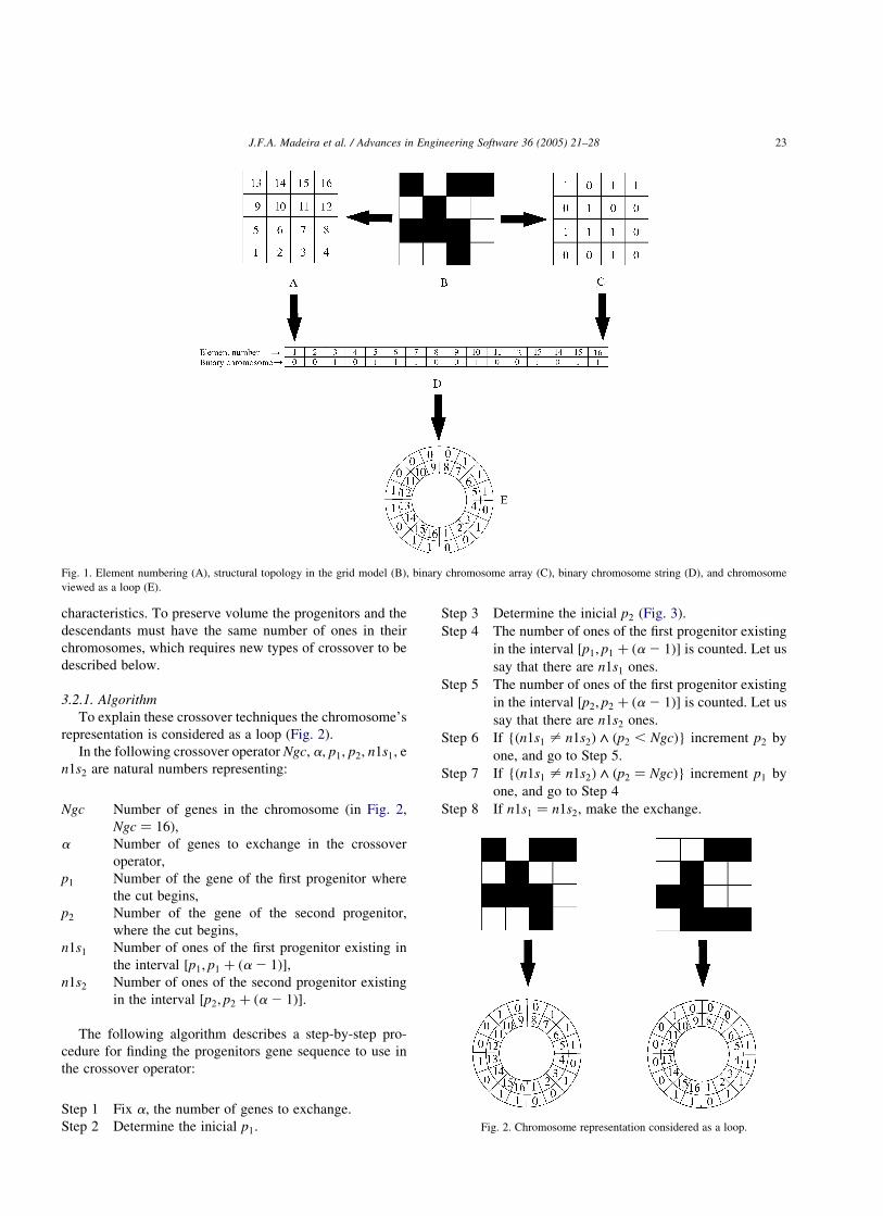
Step 3 Determine the inicial p2 (Fig. 3).

Step 4 The number of ones of the first progenitor existing

in the interval ½p1; p1 þ ða2 1Þ� is counted. Let us

say that there are n1s1 ones.

Step 5 The number of ones of the first progenitor existing

in the interval ½p2; p2 þ ða2 1Þ� is counted. Let us

say that there are n1s2 ones.

Step 6 If {ðn1s1 – n1s2Þ ^ ðp2 , NgcÞ} increment p2 by

one, and go to Step 5.

Step 7 If {ðn1s1 – n1s2Þ ^ ðp2 ¼ NgcÞ} increment p1 by

one, and go to Step 4

Step 8 If n1s1 ¼ n1s2; make the exchange.

Fig. 2. Chromosome representation considered as a loop.

Fig. 1. Element numbering (A), structural topology in the grid model (B), binary chromosome array (C), binary chromosome string (D), and chromosome

viewed as a loop (E).

J.F.A. Madeira et al. / Advances in Engineering Software 36 (2005) 21–28 23

3.2.2. Types of crossover with this technique

In the Step 2 and Step 3, the determination of p1 and p2

leads to three possible types of crossover: description

Type 1 Start with p1 ¼ p2 ¼ fixed value; for all the

evolution.

Type 2 Start with p1 ¼ p2 ¼ random value; this value to

be determined whenever the operator is used.

Type 3 p1 and p2 are determined by an independent

random choice

. In the first type, whenever two individuals cross their

descendants will always be the same. In the second type, the

probability to get the same descendants is smaller, so we

have a bigger diversity of descendants than in the previous

one. The third type gives a higher diversity in the

descendant population compared with the previous ones

and is by this reason the one used in Section 6.

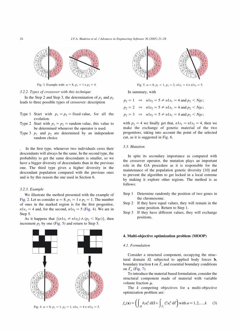
3.2.3. Example

We illustrate the method presented with the example of

Fig. 2. Let us consider a ¼ 8; p1 ¼ 1 e p2 ¼ 1: The number

of ones in the marked region is for the first progenitor,

n1s1 ¼ 4 and, for the second, n1s2 ¼ 5 (Fig. 4). We are in

Step 5.

As it happens that {ðn1s1 – n1s2Þ ^ ðp2 , NgcÞ}; then

increment p2 by one (Fig. 5) and return to Step 5.

In summary, with

p2 ¼ 1 ) n1s2 ¼ 5 – n1s1 ¼ 4 and p2 , Ngc;

p2 ¼ 2 ) n1s2 ¼ 5 – n1s1 ¼ 4 and p2 , Ngc;

p2 ¼ 3 ) n1s2 ¼ 5 – n1s1 ¼ 4 and p2 , Ngc;

with p2 ¼ 4 we finally get that, n1s1 ¼ n1s2 ¼ 4; then we

make the exchange of genetic material of the two

progenitors, taking into account the point of the selected

cut, as it is suggested in Fig. 6.

3.3. Mutation

In spite its secondary importance as compared with

the crossover operator, the mutation plays an important

role in the GA procedure as it is responsible for the

maintenance of the population genetic diversity [10] and

to prevent the algorithm to get locked in a local extreme

by making it explore other regions. The method is as

follows:

Step 1 Determine randomly the position of two genes in

the chromosome.

Step 2 If they have equal values, they will remain in the

same position. Return to Step 1.

Step 3 If they have different values, they will exchange

positions.

4. Multi-objective optimization problem (MOOP)

4.1. Formulation

Consider a structural component, occupying the struc-

tural domain V; subjected to applied body forces b;

boundary traction t on Gt and essential boundary conditions

on Gu (Fig. 7).

To introduce the material based formulation, consider the

structural component made of material with variable

volume fraction m:

The k competing objectives for a multi-objective

optimization problem are:

faðxÞ ¼ðV

biuai dVþ

ðGt

tai uai dG

� �witha¼ 1;2;…;k ð3Þ

Fig. 5. a ¼ 8; p1 ¼ 1; p2 ¼ 2; n1s1 ¼ 4 e n1s2 ¼ 5:

Fig. 4. a ¼ 8; p1 ¼ 1; p2 ¼ 1; n1s1 ¼ 4 e n1s2 ¼ 5:

Fig. 3. Example with: a ¼ 8; p1 ¼ 1 e p2 ¼ 4:


where faðxÞ with a ¼ 1; 2;…; k represents the compliance

(equivalent to the energy norm of the total displacement) for

the load case a (boundary traction ta and body forces b) and

where ua is the respective displacement field.

The multi-objective optimization problem is:

Minimize fðxÞ ¼ ðf1ðxÞ; f2ðxÞ;…; fkðxÞÞ [ Y; ð4Þ

where x ¼ ðx1; x2;…; xnÞ [ X (decision space) and Y is the

objective space, fðxÞ the multi-objective vector, and fjðxÞ the

jth objective function.subjected to the volume constraint,ðVm dV ¼ vol ð5Þ

and where the displacement ua is the solution of the integral

equilibrium equation, in virtual displacement form,ðV

Eijkmðm; qÞeijðuaÞekmðwÞ2 biwi dV2

ðGt

tai wi dG

¼ 0; ;w admissible: ð6Þ

5. Computational model

A flow chart of the general procedure for a optimization

problem with two objectives is outlined in Fig. 8

5.1. Populations

Assuming that the initial population has N individuals

and MOOP has K competing objectives, the initial

population is determined by the following procedure:

(i) Solve K single-objective problems to determine the K

optimal solutions for each objective, such that:

necessary conditions for the optimum are derived

analytically, approximated numerically through a

suitable finite element discretization and solved by a

first order method based on the optimization problem.

(ii) The initial population is formed by these K optimal

solutions of the single-objective problems and by

ðN 2 KÞ different individuals randomly generated.

Hence, the initial population has N different individuals.

Fig. 6. Crossover example.

Fig. 7. General problem of elasticity. Fig. 8. Numerical model flow chart.


To achieve low memory demand and computational

effort reduction, the algorithm does not allow two equal

individuals to be present in the population.

5.2. Finite element method (FEM) and parallel processing

Using the finite element method, the work of the external

loads is calculated for each objective. As the work of the

external loads can be calculated independently for each

individual parallel processing was used in its evaluation.

5.3. Fitness assignment, new population for mating

and selection

The concept of calculating an individual’s fitness on the

basis of Pareto dominance was first suggested in Ref. [8].

First, a ranking strategy based in non-domination properties

is used [3], that is, the non-dominated solution receives

the rank 1 (front 1), then a new non-domination test is made

in the population without these solutions and the new non-

dominated solution receives the rank 2 (front 2). This

procedure is repeated until all solutions are ranked. Second,

the rank of an individual determines its fitness value. It is

worth remarking the fact that individual fitness is related to

the whole population.

In order to avoid a possible premature convergence to a

population where only non-dominated individuals (of front

1) exist, it is imposed that the new population for matting

will be constituted by individuals of several fronts. A

geometric function, proposed in Ref. [5], the NSGA-II

method, is employed for this purpose. This function is

governed by a reduction factor r , 1 which leads to the

introduction of a greater diversity in the population. Let the

number of fronts to use be given by K; the total number of

individuals in the population be N; then the number of

individuals ni in each front i is given by Eq. (7)

ni ¼ N1 2 r

1 2 rKri21 ð7Þ

The mating individuals, in each front, are selected by the

Clustering Method [6] and a tournament selection based in

ranking position is used.

5.4. Population check and new descendants

After crossover and mutation, it is verified if the

descendants already exist in the population and, if they

do, they are eliminated to prevent unnecessary calculations.

The new descendants are finally obtained.

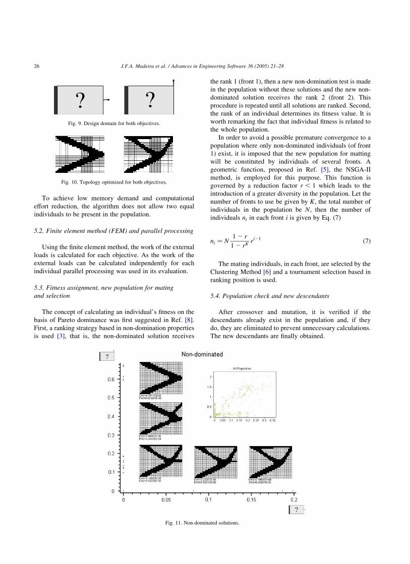
Fig. 9. Design domain for both objectives.

Fig. 10. Topology optimized for both objectives.

Fig. 11. Non-dominated solutions.


6. Examples

To test the model, two numerical examples were solved.

The optimization problem, for these two numerical

examples, is:

Minimize fðxÞ ¼ ðf1ðxÞ; f2ðxÞÞ; ð8Þ

where x ¼ ðx1; x2Þ; f1ðxÞ and f2ðxÞ are the objective

functions, representing the compliance (or external work

(EW)) for different boundary tractions, subjected to the

volume constraint (5).

In the subsequent examples, the domain has 40 £ 30 cm

and is discretized with 768 (24 £ 32) isoparametric Q8

plane stress finite elements.

The unit cell material is assumed isotropic with Young’s

modulus equal to 210 £ 109 Pa and Poisson coefficient

equal to 0.3.

The material volume is approximately 30% of the total

design volume as a result of employing a chromosome of

length 768 bits with 236 ‘ones’ and 532 ‘zeros’. The explicit

introduction of the volume equality constraint in the

chromosome de_finition lead in the examples to a reduction

of the search possibilities from <10232 to <10205, a non

negligible improvement in relative terms. The new

crossover and mutation operators were designed to exploit

this advantage.

6.1. Example 1

For the present example, domain geometry and boundary

conditions are shown in Fig. 9.

Loading conditions for both of the two objectives are also

presented in the same figure. Two load cases are considered

in the present application, for each one of the objectives:

1. A point load in the x direction with a magnitude of

200 N, for the first objective.

2. A point load in the y direction with a magnitude of

200 N, for the second objective.

Initially, the proposed single-objective problems were

solved, and the resulting solutions, for each one of the

objectives are, respectively (Fig. 10):

These single-objective optimal solutions were introduced

in the initial population. The initial population was

composed of 200 individuals (in each generation only 100

individuals were selected for matting). The solutions

obtained after 600 generations are presented in Fig. 11.

To assess the influence of the introduction of single

objective solutions in the initial population, this example

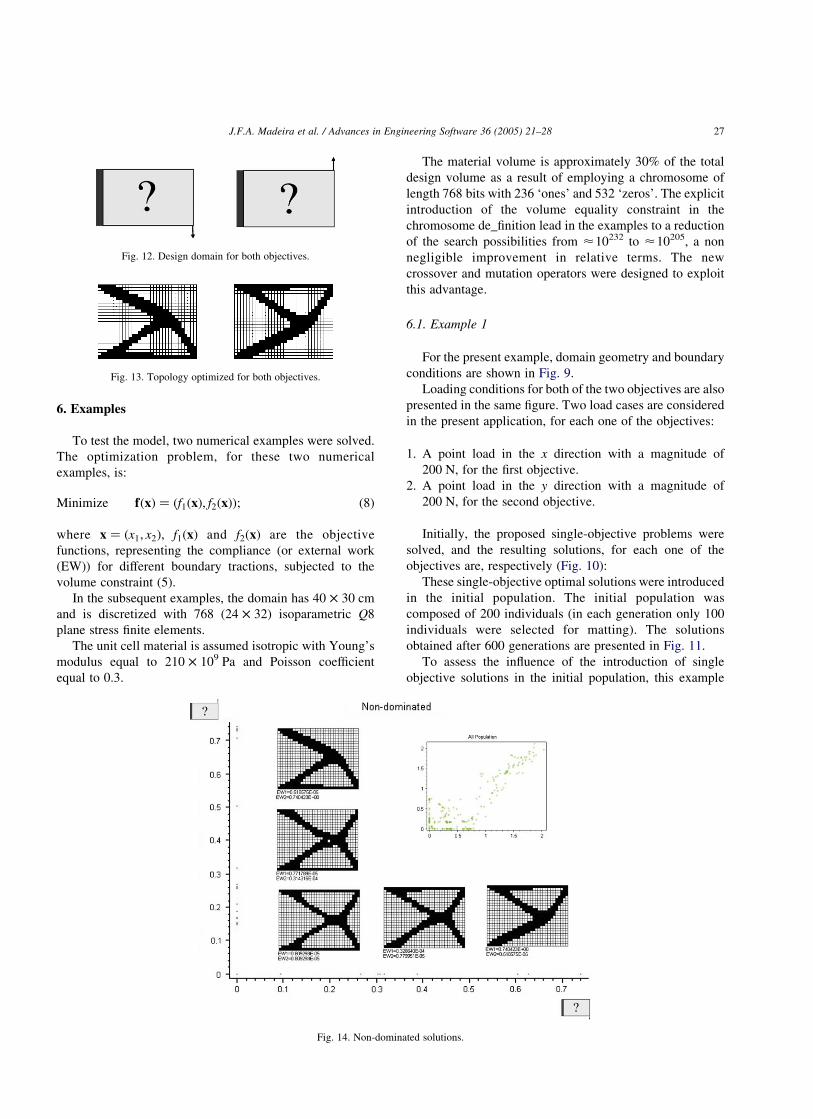
Fig. 13. Topology optimized for both objectives.

Fig. 12. Design domain for both objectives.

Fig. 14. Non-dominated solutions.


was tested with two different initial populations: (1) totally

random and (2) with single objective solutions introduced.

With a chromosome of length 128 bits (128 isoparametric

Q8 plane stress finite elements) and a volume constraint of

30% (52 ‘ones’) the results obtained at generation 15, with

single objective solutions introduced in the initial popu-

lation, were better than those obtained with a totally random

initial population at generation 500. This benefit improves

with problem size and thus this feature was retained in all

subsequent analysis.

6.2. Example 2

For the present example, the domain geometry and

boundary conditions are shown in Fig. 12.

Loading conditions for both of the two objectives are also

presented at the same figure. Two load cases are considered

in the present application, for each one of the objectives:


2200 N, for the first objective.


200 N, for the second objective.

Initially, the proposed single-objective problems were

solved, and the resulting solutions, for each one of the

objectives are, respectively (Fig. 13):

These single-objective optimal solutions were intro-

duced in the initial population. The initial population

was composed of 200 individuals (in each generation

only 100 individuals were selected for matting). The

solutions obtained after 600 generations are presented in

Fig. 14.

7. Conclusion and future work

A new method was presented and applied to a special

type of chromosome which was defined and for which it was

necessary to create new operators of crossover and

mutation.

To reduce computational effort, a priori optimal solutions

for each of the single-objective problems were introduced in

the initial population.

The volume constraint is automatically verified due to

the chromosome information structure and to the special

crossover and mutation operators developed.

In the future we intend to extend the present algorithm to

the three-dimensional case, to compare the solutions so

obtained with those available from classic methodologies

and to develop new crossover and mutation operators

applicable to this type of problems.

Acknowledgements

This work was supported by Portuguese Foundation for

Science and Technology through: Project POC-

TI/EME/43531/99. Partial support from project RTA P129

is also gratefully acknowledge.

References

[1] Chapman CD, Saitou K, Jakiela MJ. Genetic Algorithms as an

Approach to Configuration and Topology Design. ASME J Mech Des

1994;.

[2] Cohon JL. Multiobjective programming and planning. Math Sci

Engng, vol. 140. London: Academic Press, Inc; 1978.

[3] Deb K. Evolutionary algorithms for multi-criterion optimization in

engineering design. Proceedings of Evolutionary Algorithms in

Engineering and computer Science, (EUROGEN’99); 1999.

[4] Deb K, Pratap A, Agrawal S, Meyarivan T. A fast elitist non-

dominated sorting genetic algorithm for multi-objective: NSGA-II.

Proceedings of the Parallel Problem Solving from Nature VI

conference 2000;846–58.

[5] Deb K, Goel T. Controlled elitist non-dominated sorting genetic

algorithms for better convergence. Evolutionary multi-criterion

optimization, EMO, Berlin: Springer; 2001. pp. 67–81.

[6] Deb K. Multi-objective optimization using evolutionary algorithms.

London: Wiley; 2002.

[7] Fonseca CM, Fleming PJ. Genetic algorithms for multi-objective

optimization: formulation, discussion, and generalization. Proceed-

ings of the Fifth International Conference on Genetic Algorithms

1993;416–23.

[8] Goldberg DE. Genetic algorithms in search, optimization, and

machine learning, reading. Massachusetts: Addison Wesley; 1989.

[9] Hajela P. Genetic algorithms in structural topology optimization,

topology design of structures. NATO Advanced Research Workshop,

Sesimbra, Portugal; 1992.

[10] Holland J. Adaptation in natural and artificial systems. Ann Arbor:

University of Michigan Press; 1975.

[11] Horn J, Nafploitis N, Goldberg DE. A niched Pareto genetic algorithm

for multi-objective optimization. In proceedings of the First IEEE

Conference on Evolutionary Computation, IEEE World Congress on

Computational Intelligence, 1, 1994, 82–87.

[12] Knowles J, Corne D. The Pareto archived evolution strategy: a new

baseline algorithm for multi-objective optimization. Proceedings of

the Congress on Evolutionary Computation, Piscataway, NewJersey:

IEEE Service Center; 1999. pp. 98–105.

[13] Miettinen KM. Nonlinear multiobjective optimization. Norwell,

Massachusetts 02061 USA: Kluwer Academic Publishers; 1999.

[14] Pareto V. Cours D’Economie Politique, Vol. I and II, Rouge F.,

Lausanne; 1896.

[15] Schaffer JD. Multiple objective optimization with vector evaluated

genetic algorithms. PhD Thesis, Vanderbilt University; 1984.

[16] Schaffer JD. Multiple objective optimization with vector evaluated

genetic algorithms and their applications. Proceedings of the First

International Conference on Genetic Algorithms; 1985. pp. 93–100.

[17] Srinivas N, Deb K. Multi-objective funcion optimization using non-

dominated sorting genetic algorithms. Evol Comput 1995;(2):

221–48.

[18] Zitzler E, Theiele L. Multiobjective evolutionary algorithm: a

comparative case study and the strength Pareto approach. IEEE

Trans Evol Comput 1999;3(4):257–71.


Documents

Multi-objective optimization of structures topology by genetic algorithms