Embed Size (px)
Citation preview
Multi-Objective Optimization Problem using Grey Taguchi Method
A THESIS SUBMITTED IN PARTIAL FULFILLMENT OF THE REQUIREMENTS FOR
THE DEGREE OF
Bachelor of Technology
In
Mechanical Engineering.
By:
Rohit Anil Pathak
10503014
Under the guidance of:
Prof S.S Mahapatra
Department of Mechanical Engineering.
Department of Mechanical Engineering.
National Institute of Technology, Rourkela.
2009.
National Institute of Technology, Rourkela.
CERTIFICATE
This is to certify that the project entitled “Multi Objective Optimization Problem using Grey
Taguchi Method” submitted by Rohit Anil Pathak in partial fulfillment of the requirements for
the awards of Bachelor of Technology, NIT Rourkela (Deemed university) is an authentic work
carried out by him under my supervision and guidance.
To the best of my knowledge the matter embodied in the project has not been submitted to any
Institute/University for the award of any degree or diploma.
Date: May 13, 2009
Prof. S S Mahpatra
Dept. of Mechanical Engineering
National Institute of Technology, Rourkela.
Rourkela-8.

National Institute of Technology, Rourkela.
ACKNOWLEDGEMENT
I would like to articulate my deep gratitude to my project guide Prof. S S Mahapatra who has
always been my motivation to carry out the project.
It has been my pleasure to refer to the online resources made available by the institute without
which the compilation of the project would have been impossible.
Finally I extend my sincere gratitude to all those people who helped me in all their capacity to
complete the project in due time.
Date: 13 May 2009
Rohit Anil Pathak
Dept. of Mechanical Engineering National Institute of Technology, Rourkela.
Rourkela-8.

Multi Objective Optimization Problem using Grey Taguchi Method
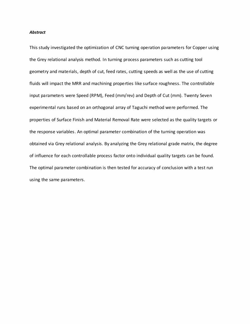
Abstract
This study investigated the optimization of CNC turning operation parameters for Copper using
the Grey relational analysis method. In turning process parameters such as cutting tool
geometry and materials, depth of cut, feed rates, cutting speeds as well as the use of cutting
fluids will impact the MRR and machining properties like surface roughness. The controllable
input parameters were Speed (RPM), Feed (mm/rev) and Depth of Cut (mm). Twenty Seven
experimental runs based on an orthogonal array of Taguchi method were performed. The
properties of Surface Finish and Material Removal Rate were selected as the quality targets or
the response variables. An optimal parameter combination of the turning operation was
obtained via Grey relational analysis. By analyzing the Grey relational grade matrix, the degree
of influence for each controllable process factor onto individual quality targets can be found.
The optimal parameter combination is then tested for accuracy of conclusion with a test run
using the same parameters.
Six Sigma Methodologies in Process Control
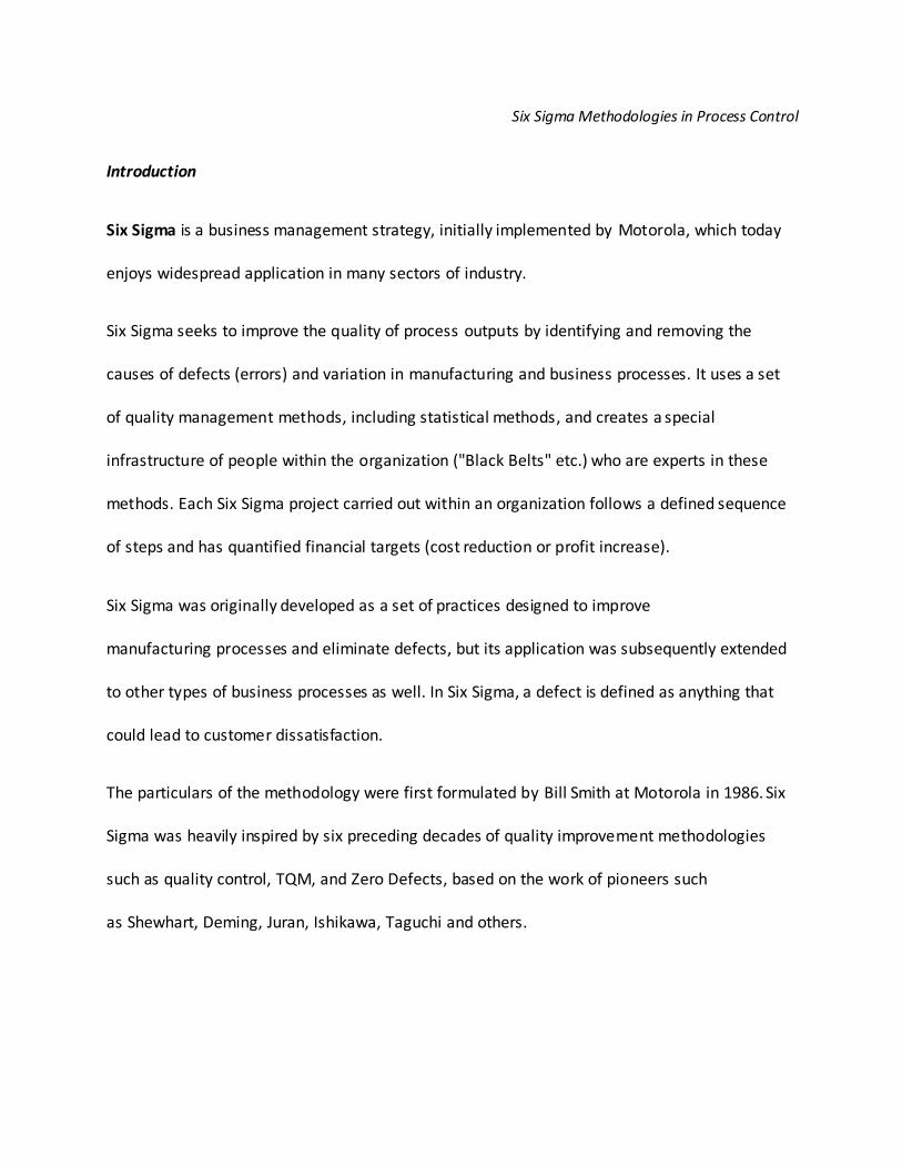
Introduction
Six Sigma is a business management strategy, initially implemented by Motorola, which today
enjoys widespread application in many sectors of industry.
Six Sigma seeks to improve the quality of process outputs by identifying and removing the
causes of defects (errors) and variation in manufacturing and business processes. It uses a set
of quality management methods, including statistical methods, and creates a special
infrastructure of people within the organization ("Black Belts" etc.) who are experts in these
methods. Each Six Sigma project carried out within an organization follows a defined sequence
of steps and has quantified financial targets (cost reduction or profit increase).
Six Sigma was originally developed as a set of practices designed to improve
manufacturing processes and eliminate defects, but its application was subsequently extended
to other types of business processes as well. In Six Sigma, a defect is defined as anything that
could lead to customer dissatisfaction.
The particulars of the methodology were first formulated by Bill Smith at Motorola in 1986. Six
Sigma was heavily inspired by six preceding decades of quality improvement methodologies
such as quality control, TQM, and Zero Defects, based on the work of pioneers such
as Shewhart, Deming, Juran, Ishikawa, Taguchi and others.
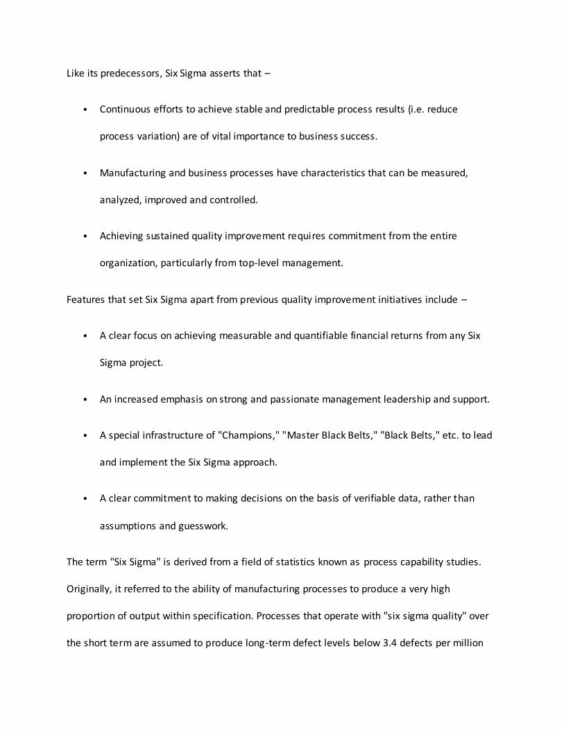
Like its predecessors, Six Sigma asserts that –
Continuous efforts to achieve stable and predictable process results (i.e. reduce
process variation) are of vital importance to business success.
Manufacturing and business processes have characteristics that can be measured,
analyzed, improved and controlled.
Achieving sustained quality improvement requires commitment from the entire
organization, particularly from top-level management.
Features that set Six Sigma apart from previous quality improvement initiatives include –
A clear focus on achieving measurable and quantifiable financial returns from any Six
Sigma project.
An increased emphasis on strong and passionate management leadership and support.
A special infrastructure of "Champions," "Master Black Belts," "Black Belts," etc. to lead
and implement the Six Sigma approach.
A clear commitment to making decisions on the basis of verifiable data, rather than
assumptions and guesswork.
The term "Six Sigma" is derived from a field of statistics known as process capability studies.
Originally, it referred to the ability of manufacturing processes to produce a very high
proportion of output within specification. Processes that operate with "six sigma quality" over
the short term are assumed to produce long-term defect levels below 3.4 defects per million
opportunities (DPMO).Six Sigma's implicit goal is to improve all processes to that level of quality
or better.
Six Sigma is a registered service mark and trademark of Motorola, Inc. Motorola has reported
over US$17 billion in savings from Six Sigma as of 2006.
Other early adopters of Six Sigma who achieved well-publicized success
include Honeywell (previously known as AlliedSignal) and General Electric, where the method
was introduced by Jack Welch. By the late 1990s, about two-thirds of the Fortune
500 organizations had begun Six Sigma initiatives with the aim of reducing costs and improving
quality.
In recent years, Six Sigma has sometimes been combined with lean manufacturing to yield a
methodology named Lean Six Sigma.
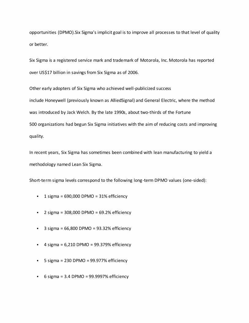
Short-term sigma levels correspond to the following long-term DPMO values (one-sided):
1 sigma = 690,000 DPMO = 31% efficiency
2 sigma = 308,000 DPMO = 69.2% efficiency
3 sigma = 66,800 DPMO = 93.32% efficiency
4 sigma = 6,210 DPMO = 99.379% efficiency
5 sigma = 230 DPMO = 99.977% efficiency
6 sigma = 3.4 DPMO = 99.9997% efficiency
These figures assume that the process mean will shift by 1.5 sigma towards the side with the
critical specification limit some time after the initial study determining the short-term sigma
level. The figure given for 1 sigma, for example, assumes that the long-term process mean will
be 0.5 sigma beyond the specification limit, rather than 1 sigma within it, as it was in the short-
term study.
Six Sigma has two key methods: DMAIC and DMADV, both inspired by Deming's Plan-Do-Check-
Act Cycle. DMAIC is used to improve an existing business process; DMADV is used to create new
product or process designs.
DMAIC
The basic method consists of the following five steps:
Define high-level project goals and the current process.
Measure key aspects of the current process and collect relevant data.
Analyze the data to verify cause-and-effect relationships. Determine what the
relationships are, and attempt to ensure that all factors have been considered.
Improve or optimize the process based upon data analysis using techniques like Design
of experiments.
Control to ensure that any deviations from target are corrected before they result in
defects. Set up pilot runs to establish process capability, move on to production, set up
control mechanisms and continuously monitor the process.
DMADV
The basic method consists of the following five steps:
Define design goals that are consistent with customer demands and the enterprise
strategy.
Measure and identify CTQs (characteristics that are Critical To Quality), product
capabilities, production process capability, and risks.
Analyze to develop and design alternatives, create a high-level design and evaluate
design capability to select the best design.
Design details, optimize the design, and plan for design verification. This phase may
require simulations.
Verify the design, set up pilot runs, implement the production process and hand it over
to the process owners.
DMADV is also known as DFSS, an abbreviation of "Design For Six Sigma".
Multi-Objective Optimization Problem
In modern industry the goal is to manufacture low cost, high quality products in a short time.
Automated and flexible manufacturing systems for that purpose along with computer
numerical control machines are capable of achieving very high accuracy and very low
processing time. Furthermore, in order to produce any product with desired quality by
machining, cutting parameters should be selected properly.
In turning process parameters such as cutting tool geometry and materials, the materials, the
depth of cut, feed rates, cutting speeds as well as the use of cutting fluids will impact the MRR
and machining qualities like surface roughness.
Planning the experiments through the Taguchi method has been quite successfully
implemented in process optimization. Therefore the study intends to apply the Taguchi method
to plan the experiments on a turning operation.
The study is to investigate the optimization of CNC turning operation parameters using the Grey
Relational Analysis method. The optimum parameters to obtain the best surface finish need to
be ascertained for this specific turning operation.
Here we shall employ statistical methods to a turning operation. There are a lot of different
parameters affecting surface finish and material removal rate like speed, feed and depth of cut.
The parameters have to be controlled in a way such that DPMO (Defect per million output) is
around three and the six sigma process is obtained. We therefore will find out the best
parameter settings in a CNC turning operation.
The surface properties of roughness average and material removal rate (MRR) are selected a s
quality targets or the response variables.
The controlled parameters are Speed, feed and depth of cut. The response variables with
respect to the controlled parameters behave as indicated below.
Surface finish increases if a.) Feed increases b.) Depth of cut decreases c.)Speed decreases.
Material Removal Rate increases if a.) Feed increases b.) Depth of cut increases c.) Surface
finish increases, and vice versa.
An optimal parameter combination of the turning operation will be found out via the Grey
Relational Analysis. By analyzing the Grey relational matrix, the degree of influence for each
controllable factor onto each quality target can also be ascertained.
Grey Relational Analysis
1. Data Preprocessing
Grey data processing must be performed before Grey correlation coefficients can be calculated.
A series of various units must be transformed to be dimensionless. Usually, each series is
normalized by dividing the data in the original series by their average.
Let the original reference sequence and sequence for comparison be represented as xo(k) and
xi(k), i=1, 2, . . .,m; k=1,2, . . ., n, respectively, where m is the total number of experiment to be
considered, and n is the total number of observation data. Data preprocessing converts the
original sequence to a comparable sequence. Several methodologies of preprocessing data can
be used in Grey relation analysis, depending on the characteristics of the original sequence
(Deng, 1989; Gau et al., 2006; You et al., 2007).
If the target value of the original sequence is “the-larger-the-better”, then the original
sequence is normalized as follows.
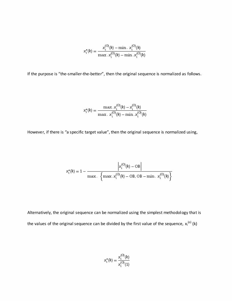
If the purpose is “the-smaller-the-better”, then the original sequence is normalized as follows.
However, if there is “a specific target value”, then the original sequence is normalized using,
Alternatively, the original sequence can be normalized using the simplest methodology that is
the values of the original sequence can be divided by the first value of the sequence, xi(o) (k)
Where, xi(o) (k) is the original sequence, xi
* (k), the sequence afer data preprocessing, max, xi(o)
(k), the largest value of , xi(o) (k) and min , xi
(o) (k), the smallest value of , xi(o) (k).
2. Grey Relational Coefficients and Grey Relational Grades
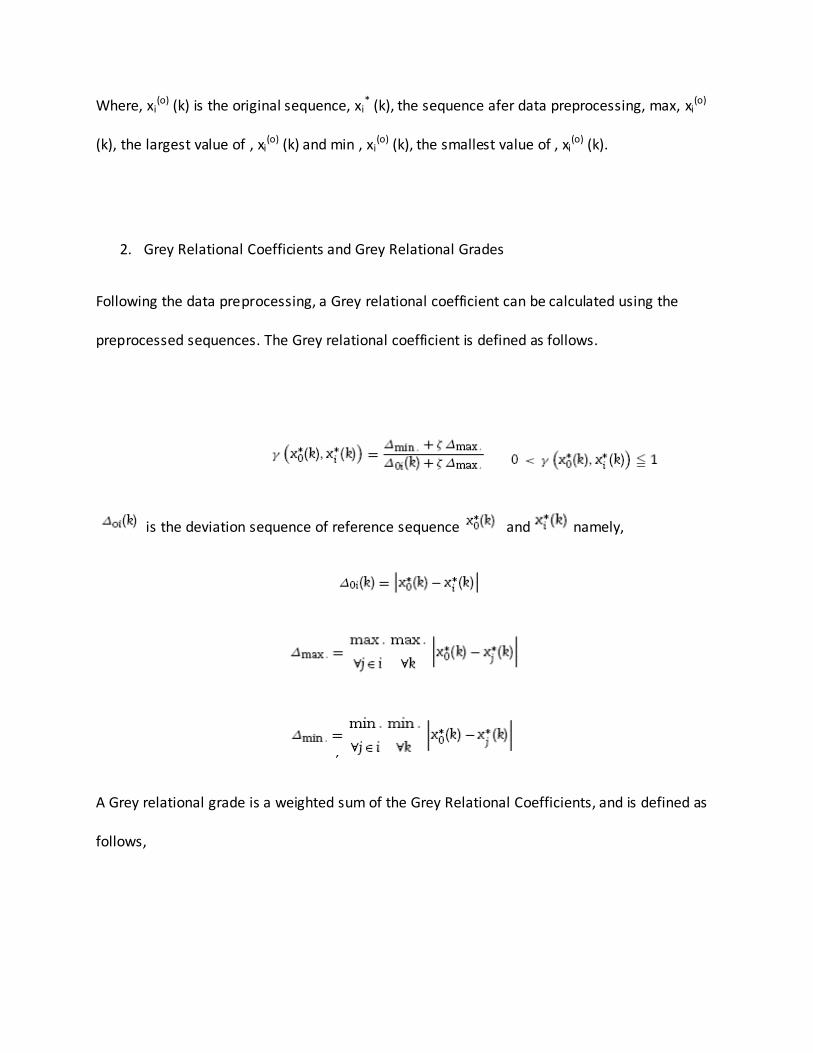
Following the data preprocessing, a Grey relational coefficient can be calculated using the
preprocessed sequences. The Grey relational coefficient is defined as follows.
is the deviation sequence of reference sequence and namely,
,
A Grey relational grade is a weighted sum of the Grey Relational Coefficients, and is defined as
follows,
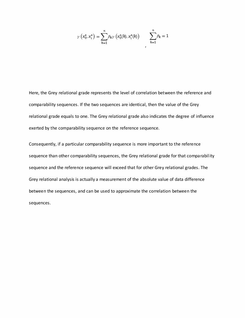
,
Here, the Grey relational grade represents the level of correlation between the reference and
comparability sequences. If the two sequences are identical, then the value of the Grey
relational grade equals to one. The Grey relational grade also indicates the degree of influence
exerted by the comparability sequence on the reference sequence.
Consequently, if a particular comparability sequence is more important to the reference
sequence than other comparability sequences, the Grey relational grade for that comparabil ity
sequence and the reference sequence will exceed that for other Grey relational grades. The
Grey relational analysis is actually a measurement of the absolute value of data difference
between the sequences, and can be used to approximate the correlation between the
sequences.
Experimental Procedure and test results
Materials
Copper is easily worked, being both ductile and malleable. The ease with which it can be drawn
into wire makes it useful for electrical work in addition to its excellent electrical properties.
Copper can be machined, although it is usually necessary to use an alloy for intricate parts, such
as threaded components, to get really good machinability characteristics. Good thermal
conduction makes it useful for heat sinks and in heat exchangers. Yield stress of copper is 55-
330 MPa and a Young’s Modulus of 110-128 GPa and a hardness of 40 HRC. In this study, to
properly control the depth of cut, the diameter of the work pieces has been fixed at 20mm for
copper bars. Kerosene was used as a coolant for the operation.
Schematic of machining
In this study, the experiments were carried out on a rigid CNC turning center with a 2 hp spindle
motor at 4200rpm (machine type of Pinacho||). Fig. 1 shows the turning operation and the
cutting length of work piece is 50 mm. At the same time, the cutter tool is K-20 HSS.
Furthermore, the cutting speed (m/min), the feed rate (mm/rev), and the depth of cut (mm)
are regulated in this experiment of turning operations.
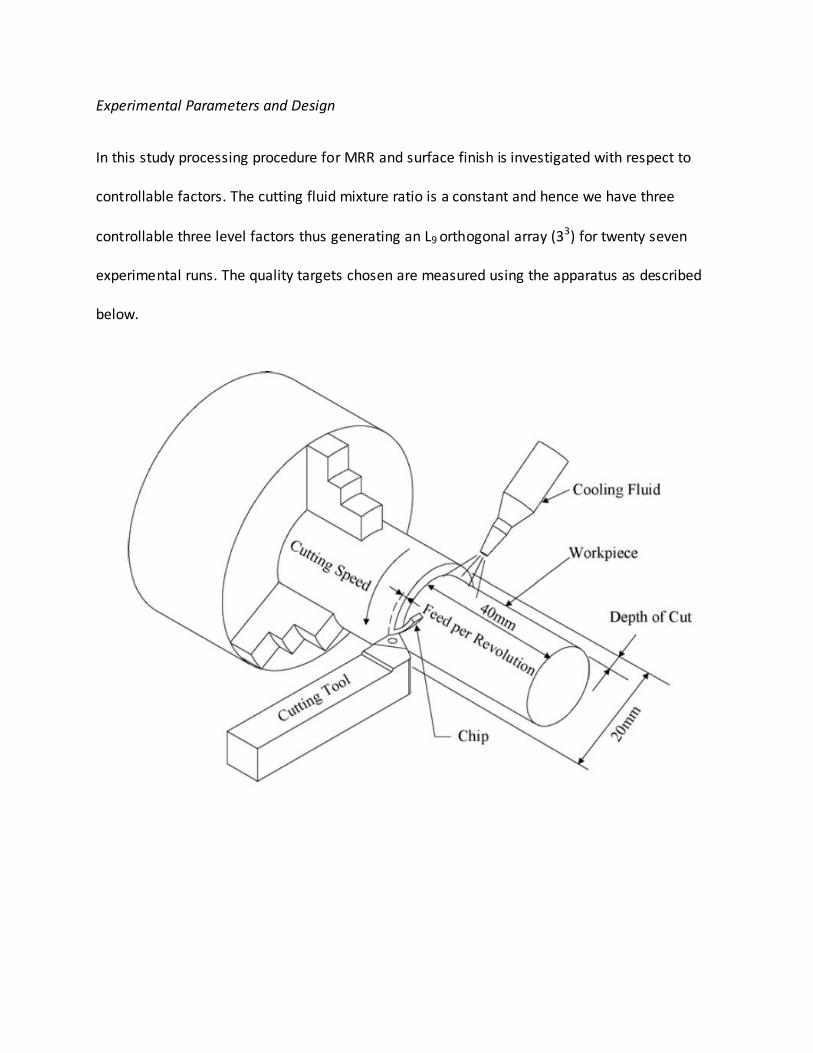
Experimental Parameters and Design
In this study processing procedure for MRR and surface finish is investigated with respect to
controllable factors. The cutting fluid mixture ratio is a constant and hence we have three
controllable three level factors thus generating an L9 orthogonal array (33) for twenty seven
experimental runs. The quality targets chosen are measured using the apparatus as described
below.
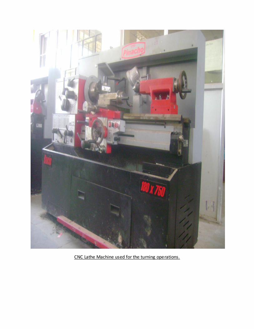
CNC Lathe Machine used for the turning operations.
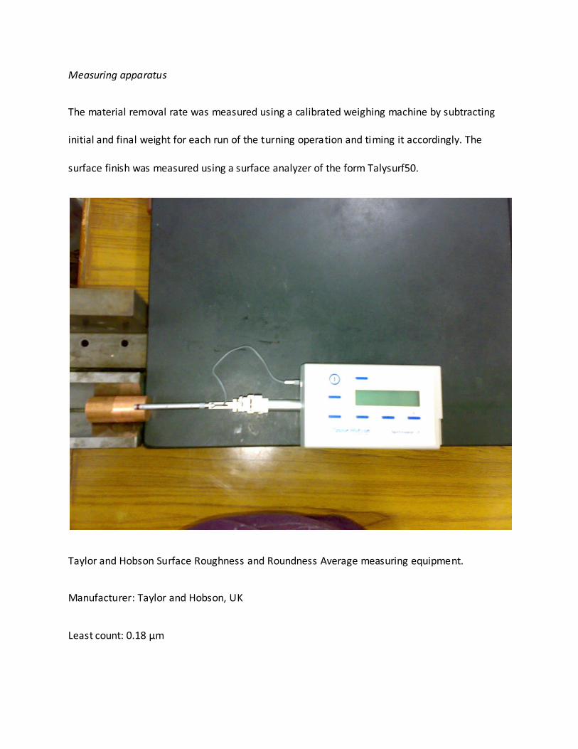
Measuring apparatus
The material removal rate was measured using a calibrated weighing machine by subtracting
initial and final weight for each run of the turning operation and timing it accordingly. The
surface finish was measured using a surface analyzer of the form Talysurf50.
Taylor and Hobson Surface Roughness and Roundness Average measuring equipment.
Manufacturer: Taylor and Hobson, UK
Least count: 0.18 µm
The experimental runs
The controllable input parameters were
Speed (RPM): 360, 530, and 860
Feed: 0.052, 0.066, and 0.083
Depth of Cut: 0.5, 0.35 and 0.2
The response variables were Material Removal Rate and Surface Finish. The tabulation for the
same is indicated.
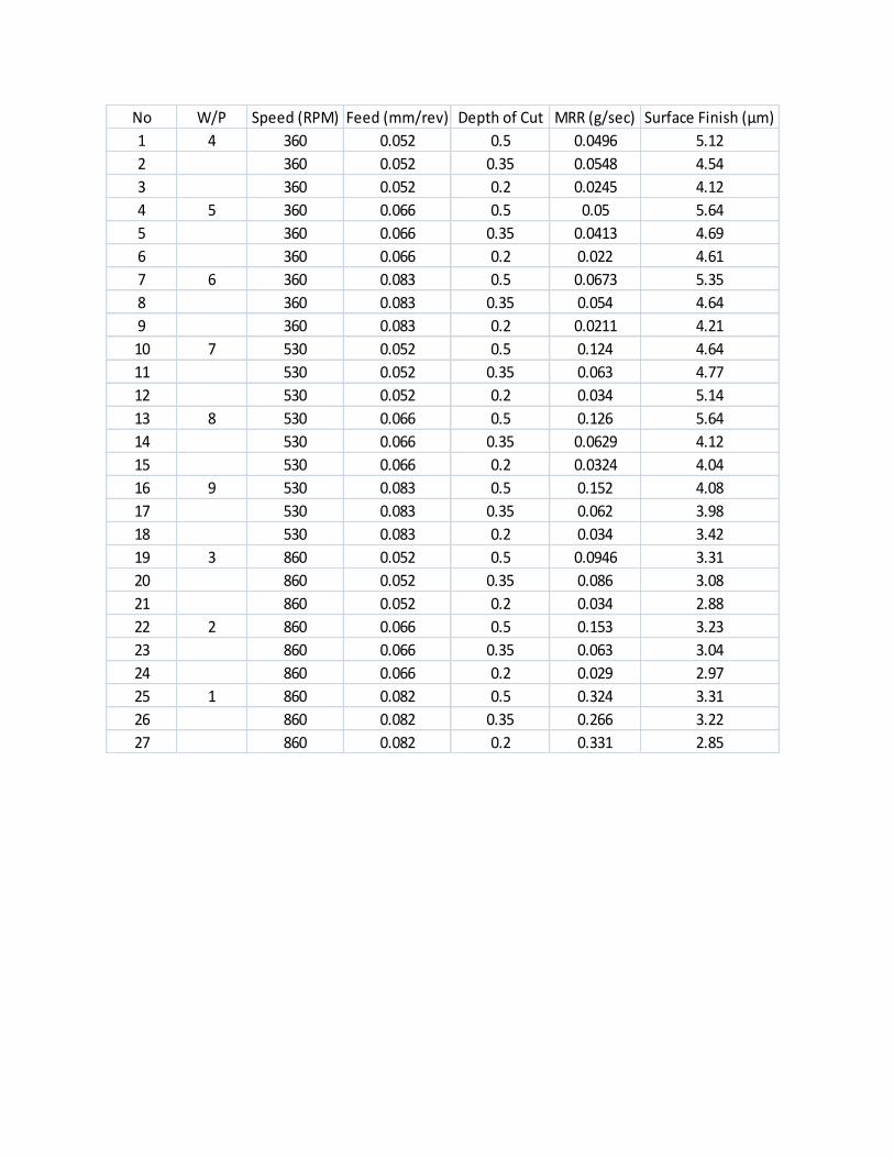
No W/P Speed (RPM) Feed (mm/rev) Depth of Cut MRR (g/sec) Surface Finish (µm)
1 4 360 0.052 0.5 0.0496 5.12
2 360 0.052 0.35 0.0548 4.54
3 360 0.052 0.2 0.0245 4.12
4 5 360 0.066 0.5 0.05 5.64
5 360 0.066 0.35 0.0413 4.69
6 360 0.066 0.2 0.022 4.61
7 6 360 0.083 0.5 0.0673 5.35
8 360 0.083 0.35 0.054 4.64
9 360 0.083 0.2 0.0211 4.21
10 7 530 0.052 0.5 0.124 4.64
11 530 0.052 0.35 0.063 4.77
12 530 0.052 0.2 0.034 5.14
13 8 530 0.066 0.5 0.126 5.64
14 530 0.066 0.35 0.0629 4.12
15 530 0.066 0.2 0.0324 4.04
16 9 530 0.083 0.5 0.152 4.08
17 530 0.083 0.35 0.062 3.98
18 530 0.083 0.2 0.034 3.42
19 3 860 0.052 0.5 0.0946 3.31
20 860 0.052 0.35 0.086 3.08
21 860 0.052 0.2 0.034 2.88
22 2 860 0.066 0.5 0.153 3.23
23 860 0.066 0.35 0.063 3.04
24 860 0.066 0.2 0.029 2.97
25 1 860 0.082 0.5 0.324 3.31
26 860 0.082 0.35 0.266 3.22
27 860 0.082 0.2 0.331 2.85
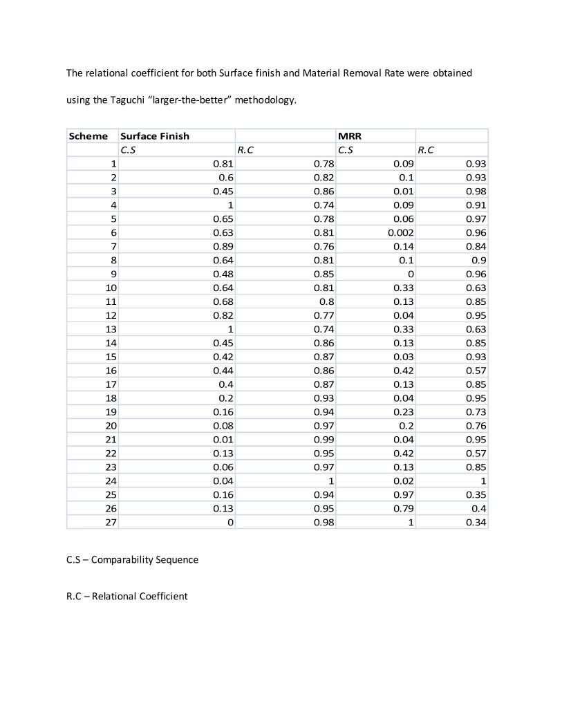
The relational coefficient for both Surface finish and Material Removal Rate were obtained
using the Taguchi “larger-the-better” methodology.
Scheme Surface Finish MRR
C.S R.C C.S R.C
1 0.81 0.78 0.09 0.93
2 0.6 0.82 0.1 0.93
3 0.45 0.86 0.01 0.98
4 1 0.74 0.09 0.91
5 0.65 0.78 0.06 0.97
6 0.63 0.81 0.002 0.96
7 0.89 0.76 0.14 0.84
8 0.64 0.81 0.1 0.9
9 0.48 0.85 0 0.96
10 0.64 0.81 0.33 0.63
11 0.68 0.8 0.13 0.85
12 0.82 0.77 0.04 0.95
13 1 0.74 0.33 0.63
14 0.45 0.86 0.13 0.85
15 0.42 0.87 0.03 0.93
16 0.44 0.86 0.42 0.57
17 0.4 0.87 0.13 0.85
18 0.2 0.93 0.04 0.95
19 0.16 0.94 0.23 0.73
20 0.08 0.97 0.2 0.76
21 0.01 0.99 0.04 0.95
22 0.13 0.95 0.42 0.57
23 0.06 0.97 0.13 0.85
24 0.04 1 0.02 1
25 0.16 0.94 0.97 0.35
26 0.13 0.95 0.79 0.4
27 0 0.98 1 0.34
C.S – Comparability Sequence
R.C – Relational Coefficient
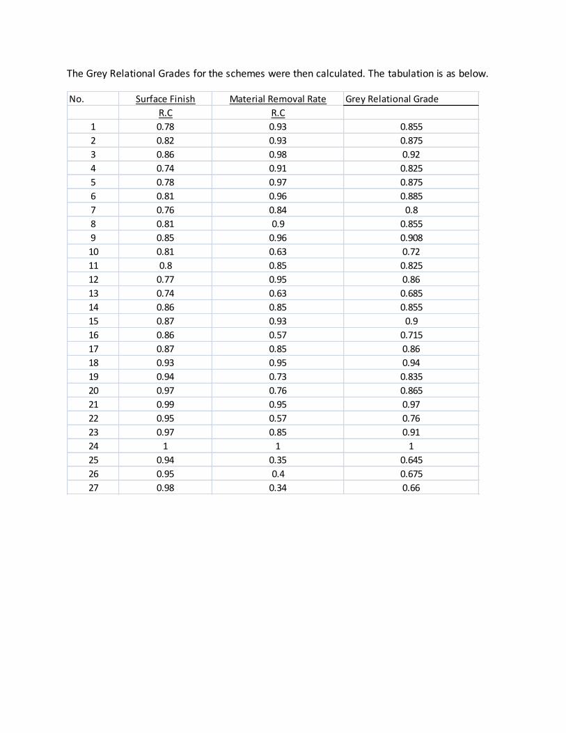
The Grey Relational Grades for the schemes were then calculated. The tabulation is as below.
No. Surface Finish Material Removal Rate Grey Relational Grade
R.C R.C
1 0.78 0.93 0.855
2 0.82 0.93 0.875
3 0.86 0.98 0.92
4 0.74 0.91 0.825
5 0.78 0.97 0.875
6 0.81 0.96 0.885
7 0.76 0.84 0.8
8 0.81 0.9 0.855
9 0.85 0.96 0.908
10 0.81 0.63 0.72
11 0.8 0.85 0.825
12 0.77 0.95 0.86
13 0.74 0.63 0.685
14 0.86 0.85 0.855
15 0.87 0.93 0.9
16 0.86 0.57 0.715
17 0.87 0.85 0.86
18 0.93 0.95 0.94
19 0.94 0.73 0.835
20 0.97 0.76 0.865
21 0.99 0.95 0.97
22 0.95 0.57 0.76
23 0.97 0.85 0.91
24 1 1 1
25 0.94 0.35 0.645
26 0.95 0.4 0.675
27 0.98 0.34 0.66
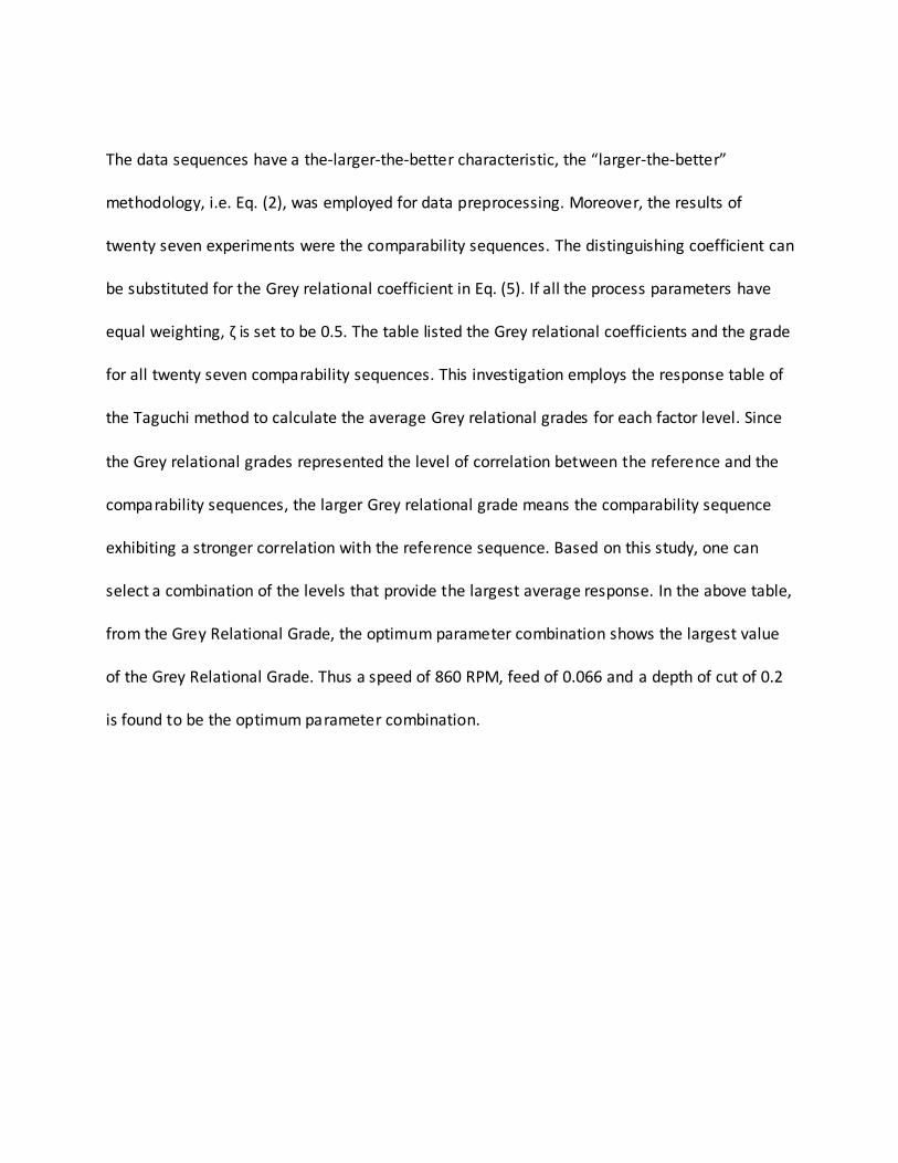
The data sequences have a the-larger-the-better characteristic, the “larger-the-better”
methodology, i.e. Eq. (2), was employed for data preprocessing. Moreover, the results of
twenty seven experiments were the comparability sequences. The distinguishing coefficient can
be substituted for the Grey relational coefficient in Eq. (5). If all the process parameters have
equal weighting, ζ is set to be 0.5. The table listed the Grey relational coefficients and the grade
for all twenty seven comparability sequences. This investigation employs the response table of
the Taguchi method to calculate the average Grey relational grades for each factor level. Since
the Grey relational grades represented the level of correlation between the reference and the
comparability sequences, the larger Grey relational grade means the comparability sequence
exhibiting a stronger correlation with the reference sequence. Based on this study, one can
select a combination of the levels that provide the largest average response. In the above table,
from the Grey Relational Grade, the optimum parameter combination shows the largest value
of the Grey Relational Grade. Thus a speed of 860 RPM, feed of 0.066 and a depth of cut of 0.2
is found to be the optimum parameter combination.
Confirmation Test / Conclusion
After identifying the most influential parameters, the final phase is to verify the Speed, Feed
and Depth of Cut by conducting the confirmation experiments. The scheme 27 is an optimal
parameter combination of the turning process via the Grey relational analysis. Therefore, the
condition scheme 27 of the optimal parameter combination of the turning process was treated
as a confirmation test. If the optimal setting with a cutting speed of 860 RPM, 0.066 mm/rev of
the feed rate, a cut depth of 0.2mm, and the surface roughness obtained is 2.97 µm and the
MRR obtained is 0.029 g/sec.
References
Aslan, E., Camuscu, N., Birgoren, B., 2007. Design optimization of cutting parameters when
turning hardened AISI 4140 steel (63 HRC) with Al2O3 +TiCN mixed ceramic tool. Mater. Des. 28.
Chen, D.C., Chen, C.F., 2007. Use of Taguchi method to study a robust design for the sectioned beams curvature during rolling. J. Mater. Process. Technol. 190, 130–137.
Chiang, K.T., Chang, F.P., 2006. Optimization of the WEDM process of particle-reinforced material with multiple performance characteristics using Grey relational analysis.
J. Mater. Process. Technol. 108, 96–101. Davim, J.P., 2003. Design of optimization of cutting
parameters for turning metal matrix composites based on the orthogonal arrays.
J. Mater. Process. Technol. 132, 340–344. Deng, J.L., 1989. Introduction to Grey system theory. EI Baradie, M.A., 1996. Cutting fluids: part I characterization.
Fung, C.P., Kang, P.C., 2005. Multi-response optimization in friction properties of PBT
composites using Taguchi method and principle component analysis. Fung, C.P., Huang, C.H., Doong, J.L., 2003. The study on the optimization of injection molding
process parameters with Gray relational analysis.
Kalpakjian, S., Schmid, S.R., 2001. Manufacturing Engineering and Technology, International, Fourth ed. Prentice Hall Co.,
New Jersey, pp. 536–681.
Lin, C.L., 2004. Use of the Taguchi method and Grey relational analysis to optimize turning operations with multiple performance characteristics. Mater. Manuf. Process. 19 (2), 209–220. Acknowledgments I would like to thank the following people for their assistance in the course of my project Mr. S Samal, Central Workshop
Mr S. Das, Central Workshop Mr. Ali Mir Ayub, Central Workshop Mr. Kunal Nayak, Technical Assistant, ME