Multi-Product Firms and Flexible Manufacturing

in the Global Economy�

Carsten Eckely

University of Bamberg

J. Peter Nearyz

University of Oxford and CEPR

April 8, 2009

Abstract

We present a new model of multi-product �rms (MPFs) and �exible manufacturing, and explore

its implications in partial and general oligopolistic equilibrium. Globalization a¤ects the scale and

scope (or intensive margin and intra-�rm extensive margin) of MPFs through a competition e¤ect

and a demand e¤ect. The model highlights a new source of gains from trade: productivity increases

as �rms become "leaner and meaner", concentrating on their core competence; but also a new source

of losses from trade: product variety may fall. Our results also hold under free entry, which allows

in addition for adjustment along the traditional inter-�rm extensive margin.

Keywords: Flexible Manufacturing, General Oligopolistic Equilibrium (GOLE), International

Trade, Multi-Product Firms, Product Diversity.

JEL Classi�cation: F12, L13

�We thank the editor, Andrea Prat, and two anonymous referees, as well as Andy Bernard, David Greenstreet, VolkerGrossmann, Victor Norman, Jim Rauch, Steve Redding, Nicolas Schmitt, and participants in various seminars, at ETSG2005 in Dublin, and at the Winter 2005 Meetings of the NBER International Trade and Investment Program in Palo Altofor helpful comments. Carsten Eckel thanks the German Science Foundation (DFG grant number EC 216/4-1) for researchsupport.

yDepartment of Economics, University of Bamberg, Feldkirchenstr. 21, D-96052 Bamberg, Germany; tel.: (+49) 951-8632582; email: carsten.eckel@uni-bamberg.de.

zDepartment of Economics, University of Oxford, Manor Road Building, Oxford, OX1 3UQ, U.K.; tel.: (+44) 1865-271085; fax: (+44) 1865-271094; e-mail: peter.neary@economics.ox.ac.uk.

1 Introduction

Multi-product �rms are omnipresent in the modern world economy, especially in technologically advanced

countries. Their importance is documented in a recent study of U.S. �rms by Bernard, Redding and

Schott (2006a).1 This shows that multi-product �rms are present in all industries; they account for less

than half (41%) of the total number of �rms but the vast bulk (91%) of total output; and they are

very active in varying their product mix: 89% of multi-product �rms do so on average every �ve years.

Yet, despite this empirical importance, and despite the interest in trade as a source of increased product

diversity, multi-product �rms have received relatively little attention in the theory of international trade.

General equilibrium models of international trade typically rely on single-product �rms only. In such a

framework, intra-�rm adjustments are limited to changes in the scale of production. Changes in diversity

are linked exclusively to changes in the number of �rms. In contrast to the theory of international trade,

multi-product �rms have received more attention in the �eld of industrial organization. (See, for exam-

ple, Brander and Eaton (1984), Klemperer (1992), Ottaviano and Thisse (1999), Hallak (2000), Baldwin

and Ottaviano (2001), Grossmann (2003), Johnson and Myatt (2003, 2006), Ju (2003), Allanson and

Montagna (2005), and Baldwin and Gu (2005)). These studies have emphasized that, because of supply

and demand linkages, intra-�rm adjustments within multi-product �rms are signi�cantly di¤erent from

adjustments via exit and entry. However, studies in industrial organization are commonly conducted

in partial equilibrium, so that they cannot capture feedback e¤ects through factor markets.2 But given

the omnipresence and empirical importance of multi-product �rms across industries, these-general equi-

librium e¤ects can be signi�cant and should be included in an analysis of multi-product �rms in the

global economy. In this paper, we develop a new model of multi-product �rms that incorporates both

supply and demand linkages and explore its implications in partial and general oligopolistic equilibrium.

Our �ndings show that intra-�rm adjustments imply quite di¤erent predictions regarding the impact of

international trade on �rm productivity, factor prices, and product diversity than traditional models of

international trade.

The supply and demand linkages in our framework capture important di¤erences between multi-

product and single-product �rms, which have been highlighted in the theory of industrial organization

but largely neglected in the literature on international trade. First, in contrast to single-product �rms,

multi-product �rms internalize demand linkages between the varieties they produce. This feature is

called the �cannibalization e¤ect�and is generally considered a de�ning feature of multi-product �rms.

The existence of a cannibalization e¤ect requires that �rms are large in their markets and behave like

oligopolists. It gives rise to strategic interactions that are of particular importance for a �rm�s reaction

1This uses a longitudinal database derived from the U.S. Census of Manufactures with observations at �ve-yearlyintervals between 1972 and 1997. Over 140,000 surviving �rms are present in each census year. In this study a �product�is de�ned at the �ve-digit Standard Industry Classi�cation (SIC) level.

2Ottaviano and Thisse (1999) allow for labour market equilibrium in their framework, but since they use quasi-linearpreferences, they cannot address income e¤ects. The same is true of Hallak (2000) and Baldwin and Gu (2005).

1

to changes in competition. Second, the varieties within a �rm�s product line are linked on the cost

side through a �exible manufacturing technology (Milgrom and Roberts (1990), Eaton and Schmitt

(1994), Norman and Thisse (1999), Eckel (2009)). Flexible manufacturing emphasizes the fact that �rms

typically possess a �core competence� in the production of a particular variety and that they are less

e¢ cient in the production of varieties outside their core competence. In our framework, this ine¢ ciency

translates into higher marginal labor requirements. Hence, �exible manufacturing allows �rms to expand

their product lines, but this expansion is subject to diseconomies of scope and creates cost heterogeneities

between products. These cost heterogeneities are important for the general-equilibrium e¤ects of changes

in product ranges. The two types of linkages, cannibalization and �exible manufacturing, are the driving

forces behind the intra-�rm adjustments in our framework.

The nature of cost linkages and the existence of demand linkages and cannibalization distinguish our

work from recent theoretical papers by Allanson and Montagna (2005), Bernard, Redding and Schott

(2006b) and Nocke and Yeaple (2006). Allanson and Montagna assume both �rm- and variety-speci�c

�xed costs; Bernard, Redding and Schott assume that �rm- and variety-speci�c costs are random and

independent of each other; and Nocke and Yeaple assume that unit costs of all products are positively

related to the range of products produced. Even more signi�cantly, all three papers analyze multi-product

�rms in models of �large-group�monopolistic competition. In such a framework, demand linkages and

strategic behaviour are excluded, making it impossible to address the issue of cannibalization.

This paper addresses the role of adjustment processes within multi-product �rms and linkages with

factor and goods markets in a global economy. In particular, we analyze how multi-product �rms react to

di¤erent globalization shocks (distinguishing between the competition and market-size e¤ects of greater

international market integration), how these intra-�rm adjustments a¤ect the demand for labour, and

how induced changes in wages a¤ect the optimal product range and the distribution of outputs within

a �rm�s product range. In order to isolate adjustments within �rms from adjustment via exit and entry,

we focus for most of the paper on oligopolistic markets where barriers to entry are prohibitively high and

the number of �rms is exogenously given. However, we also extend our framework to allow for free entry,

and show that our main predictions continue to hold. Our analysis provides plausible explanations for

observable facts about multi-product �rms and presents testable propositions with respect to the impact

of economy-wide shocks on the scale and scope of multi-product �rms.

Section 2 introduces our assumptions about individual agents, which generate a demand for di¤eren-

tiated products by consumers, and an endogenous choice of scale and scope by �rms. Section 3 illustrates

the determination of equilibrium in a single industry spread across a number of countries, and derives

the paper�s key results on the e¤ects of globalization. Section 4 shows how these results are quali�ed and

enriched when labour market adjustment in general equilibrium is allowed. Finally, Section 5 explores

the robustness of our results when the model is extended to allow for free entry, heterogeneous �rms,

2

and partial trade liberalization. Proofs of all results are presented in the Appendix.

2 Consumers and Firms

We assume that the world economy consists of a �nite number of countries, all with fully integrated

goods markets but no international factor mobility. There is a continuum of identical industries, each

of which has an oligopolistic market structure. We begin in this section by considering the behaviour

of consumers and multi-product �rms in a single industry. This introduces the two key features of the

model: demand for di¤erentiated products on the one hand, and a �exible manufacturing technology on

the other.

2.1 Preferences and Demand

Our speci�cation of preferences combines the continuum-quadratic approach to symmetric horizontal

product di¤erentiation of Ottaviano, Tabuchi and Thisse (2002) with the absence of an outside (or

"numéraire") good as in Neary (2002). Each consumer maximizes a two-tier utility function that depends

on their consumption levels q (i) ; i 2 [1; N ], where N is the measure of di¤erentiated goods produced in

each industry z, and z varies over the interval [0; 1]. The upper tier is an additive function of a continuum

of sub-utility functions, each corresponding to one industry:

U [u fzg] =Z 1

0

u fzg dz. (1)

As for the lower tier, each sub-utility function is quadratic:

u fzg = aZ N

0

q (i) di� 12b

24(1� e)Z N

0

q (i)2di+ e

(Z N

0

q (i) di

)235 . (2)

The parameters a, b and e are assumed to be non-negative and identical for all consumers: a denotes

the consumer�s maximum willingness to pay, while e is an inverse measure of product di¤erentiation,

assumed to lie strictly between zero and one. If e = 1, the goods are homogeneous (perfect substitutes)

so that demand depends on aggregate output only. By contrast, e = 0 describes the monopoly case where

the demand for each good is completely independent of other goods. We rule out these two extreme

cases in order to focus on competition between �rms producing di¤erentiated products.

Consumers maximize utility as given by (1) and (2) subject to the budget constraint

Z 1

0

Z N

0

p (i) q (i) didz � I, (3)

where p (i) is the price of variety i and I denotes individual income. This leads to the following individual

3

inverse demand functions:

�p (i) = a� b"(1� e) q (i) + e

Z N

0

q (i) di

#. (4)

The parameter � is the Lagrange multiplier, which denotes the consumer�s marginal utility of income.

To move from individual to aggregate demands, we assume that there are L consumers located in each

of k identical countries, all with identical preferences. In addition, we assume that the goods markets

of all countries are completely integrated in a single world market and free trade prevails, so the price

of a given variety is the same everywhere. Hence the market demand for a particular variety i in any

industry, x (i), facing a �rm in any country consists of demand from all consumers, kLq (i). This allows

(4) to be rewritten as the inverse world market demand function for good i:

p (i) = a0 � b0 [(1� e)x (i) + eY ] . (5)

where a0 � a=�, b0 � b=�kL, and Y �R N0x (i) di denotes the output of the entire industry. Note that

the demand slope b0 depends inversely on the total number of consumers in the world.

Because they depend on �, the parameters a0 and b0 are endogenously determined in general equi-

librium. However, with a continuum of industries they are perceived as exogenous by individual �rms.

Hence �rms are �large� in their own market but �small� in the economy as a whole, which permits a

consistent analysis of oligopoly in general equilibrium. For convenience, and with no loss in generality, we

normalize by setting � equal to one, so in general equilibrium all nominal variables should be interpreted

as relative to the marginal utility of income. (See Neary (2002) for details.)

2.2 Costs and Technology of Multi-Product Firms

As explained in the introduction, the technology of multi-product �rms is characterized by a core com-

petence and �exible manufacturing. This is illustrated in Figure 1, where cj (i) denotes the marginal

cost which a typical �rm j incurs to produce good i.3 We assume the marginal cost is constant with

respect to the quantity produced, but varies across varieties. It is lowest for the core competence variety,

which uses the �rm�s most e¢ cient production process. We set a �rm�s core competence at i = 0 with

cj (0) = c0j . In addition to producing its core competence variety, the �rm can add new products to its

product line via �exible manufacturing, which describes its ability to produce additional varieties with

only a minimum of adaptation. However, some adaptation is necessary, so each addition to the product

line incurs a higher marginal production cost but leaves the marginal production costs of existing prod-

3Consumers are indi¤erent about which �rm produces which varieties, so the subscript j was not needed in the previoussub-section. We use it here since in Section 2.3 we consider the behaviour of a single �rm playing a Cournot game againstother �rms. Later (except in Section 5.2), we concentrate on symmetric equilibria, so we can omit it again.

4

ucts unchanged.4 The marginal production cost of variety i is therefore a strictly increasing function of

the mass of products produced: @cj(i)@i > 0, as shown. In general we do not need to impose any further

restrictions on the cj (i) function, though some results are strengthened in the linear case, cj (i) = c0j+ i,

and the diagrams assume this for ease of interpretation.

Each multi-product �rm produces a mass of products which is denoted by �j . Pro�ts for a multi-

product �rm j are then given by

�j =

Z �j

0

[pj (i)� cj (i)]xj (i) di� F , (6)

where the �xed cost F is independent of both scale and scope.

2.3 Optimal Scale and Scope

We assume that �rms play a single-stage Cournot game. Hence they simultaneously choose the quantity

produced of each good and the mass of products produced, assuming that rival �rms do not change their

scale or scope. The �rst-order condition with respect to the scale of production of a particular good i is

given by@�j@xj (i)

= pj (i)� cj (i)� b0 [(1� e)xj (i) + eXj ] = 0, (7)

where Xj �R �j0xj (i) di denotes the �rm�s aggregate output.5 Equation (7) shows that the optimal

pro�t margin on good i is proportional to a weighted average of the output of that good and the �rm�s

total output, where the weights depend on the substitution parameter e. Eliminating the price from

equations (5) and (7) gives the output of a single variety:

xj (i) =a0 � cj (i)� b0e (Xj + Y )

2b0 (1� e) . (8)

As always in Cournot competition, industry output has a negative e¤ect on equilibrium output, re�ecting

the e¤ect of greater competition from rival �rms. In addition, equation (8) shows that the �rm�s total

output Xj has a further negative e¤ect on the output of each variety, re�ecting the cannibalization e¤ect

discussed in the introduction. Because a larger output of one variety tends to lower the prices that

consumers are willing to pay for all other varieties, a multi-product �rm has an additional incentive to

restrict its output of each variety beyond the familiar own-price e¤ect. The e¤ect is illustrated in Figure

2. Because of the cannibalization e¤ect, the marginal revenue curve is lower than it would be for a

single-product �rm, so other things equal a multi-product �rm produces less of every good.

4By contrast, Bernard, Redding and Schott (2006b) assume that each �rm has a �rm-speci�c and a variety-speci�cproductivity draw, all of which are independent of each other; while Nocke and Yeaple (2006) assume that all productshave the same marginal cost, and an expansion in a �rm�s product range raises the marginal costs of all its products.

5The second-order condition is easily veri�ed:@2�j@xj(i)

2 =@pj(i)

@xj(i)� b0 (1� e)� b0e

@Xj

@xj(i)< 0.

5

Equation (8) also shows that, given its total output, a �rm produces less of each variety the further

it is from its core competence: xj (i) is decreasing in cj (i). Given the symmetric structure of demand,

this means that it must charge higher prices for products that are further from its core competence, as

can be seen by solving (5) and (7) for the price of each variety:

pj (i) =1

2[a0 + cj (i)� b0e (Y �Xj)] . (9)

This heterogeneity of prices charged across varieties is in contrast with models of multi-product �rms

where economies of scope arise from �xed costs, or where producing more varieties raises marginal costs

for all varieties, as in Nocke and Yeaple (2006). However, in our model not all of the higher costs are

passed on to consumers. Some (in fact, exactly half, because demand is linear) are absorbed by the �rm

itself in the form of lower pro�t margins on varieties that are further from its core competence:

pj (i)� cj (i) =1

2[a0 � cj (i)� b0e (Y �Xj)] (10)

Note also that, by contrast with the output equation (8), the competition and cannibalization e¤ects have

opposite signs in (9) and (10). More competition reduces the prices which �rms can charge in Cournot

markets, but this is partly (though not fully) o¤set by the cannibalization e¤ect, which encourages

multi-product �rms to charge higher prices on all their varieties, and also allows them to earn higher

margins.

Consider next the �rm�s choice of product line. Multi-product �rms add new products as long as

marginal pro�ts are positive. The �rst-order condition with respect to the scope of production is then:6

@�j@�j

= [pj (�j)� cj (�j)]xj (�j) = 0. (11)

From the �rst-order condition for scale, equation (7), the pro�t on the marginal variety pj (�j)� cj (�j)

cannot be zero. Equation (11) therefore implies that pro�t-maximizing multi-product �rms choose their

product range so that the output of the marginal variety is zero: xj (�j) = 0. Combining this with

equation (8), the �rst-order condition with respect to scope can also be expressed as

cj (�j) = a0 � b0e (Xj + Y ) . (12)

The determination of the pro�t-maximizing product range is illustrated in Figure 1. Starting from its

core competence variety, the �rm adds new varieties up to the point where the marginal cost of producing

the marginal variety equals the marginal revenue at zero output. To drive sales to zero, the price charged

6As@cj(�j)@�j

> 0 and, thus,@xj(�j)@�j

= � 12b0(1�e)

@cj(�j)@�j

< 0, the second-order condition is easily veri�ed:@2�j@�2j

=

[pj (�j)� cj (�j)]@xj(�j)@�j

< 0.

6

on its marginal variety is the highest of all its varieties, equal from (9) to pj (�j) = a0 � b0eY . However,

it earns the lowest pro�t margin on its marginal variety, though as already noted it is strictly positive,

equal from (10) and (12) to b0eXj .

2.4 Productivity of Multi-Product Firms

Our assumptions about technology imply a direct relationship between a �rm�s scope of production and its

productivity. Assume that labour is the only factor of production, and that the labour market is economy-

wide and perfectly competitive. The unit cost of producing each variety can then be decomposed into a

technological component, denoted (i), and a factor-cost component equal to the wage w: c (i) = w (i).

(From now on we omit the �rm subscript j.) Here (i) measures the labour input needed to produce a

unit of output of variety i.

Suppose now that the �rm is subject to a shock to any exogenous variable, other than the level of

technology (i.e., the function f (i)g). How do we measure the resulting change in the �rm�s productivity?

Measuring total labour input is straightforward: ignoring �xed costs, it equals the integral of the labour

requirements of each variety times its output:

l =

Z �

0

(i)x (i) di (13)

To measure the change in labour productivity ("LP") in response to an increase in some exogenous

variable �, we subtract the log-change in total labour input l from a Divisia index of the changes in

outputs of di¤erent varieties, aggregated using weights h (i) to be discussed below:

d lnLP

d ln �=

R �0h (i) dx(i)d ln �diR �

0h (i)x (i) di

� d ln l

d ln �(14)

We �rst want to show that the e¤ects on productivity of changes in any exogenous variable depend

only on their e¤ects on product scope �. To see this, combine the �rst-order conditions for scale and

scope, equations (8) and (12) respectively, to express the output of each variety in terms of the di¤erence

between its own marginal cost and that of the marginal variety:

x (i) =w [ (�)� (i)]2b0 (1� e) . (15)

Next, substituting from (15) for outputs x (i) into the variable labour demand from (13) and evaluating

the integral yields:

l =w� (�)

2b0 (1� e) , where � (�) �Z �

0

(i) [ (�)� (i)] di (16)

Here � (�) is the technological component of the �rm�s variable demand for labour. Comparing (15)

and (16), it is clear that both equal some function of technology and scope �, multiplied by a common

7

factor w2b0(1�e) . It follows that the change in productivity in (14) depends only on the e¤ect of product

scope on productivity times the e¤ect of the exogenous shock on the �rm�s equilibrium scope: d lnLPd ln � =

@ lnLP@ ln �

d ln �d ln � .

7

Consider next the choice of the weights h (i) in the Divisia index. Note �rst that if the weights are

marginal costs, h (i) = c (i), which is equivalent to input requirements, h (i) = (i), then the log-change

in output is identical to that in employment from (13), and so productivity is independent of �rm scope:

@ lnLP

@ ln �

����h(i)= (i)

=

R �0 (i) @x(i)@ ln � diR �

0 (i)x (i) di

� @ ln l

@ ln �= 0 (17)

This re�ects the fact that the technology available to the �rm is una¤ected by the shock. However, the

techniques in use are de�nitely a¤ected, so an alternative measure of productivity change which takes

account of this seems preferable. We consider two di¤erent sets of weights, h (i) = 1 and h (i) = p (i).

Weighting by prices as in the latter gives the most satisfactory measure of output and productivity

change, whereas focusing simply on the unweighted sum of outputs X as in the former gives better

intuition.

The key result for the response of productivity to changes in �rm scope can be summarized as follows:

Proposition 1 With given technology, any shock which raises the product range of a multi-product �rm:

(a) reduces productivity as measured in (14) when output is a simple aggregate, h (i) = 1; (b) reduces it

but by less when output changes are price-weighted, h (i) = p (i); and (c) leaves it unchanged when output

changes are marginal-cost-weighted, h (i) = (i).

Proofs for parts (a) and (b) are given in the Appendix, but the underlying intuition can be explained

as follows. Varieties further from the �rm�s core competence have higher labour requirements and

hence lower productivity. Therefore, when the outputs of all varieties are weighted equally as in (a),

an expansion in the �rm�s product range (even allowing for an optimal reallocation between existing

varieties) must lower measured productivity. Weighting by prices as in (b) increases the importance

attributed to marginal varieties, recalling from (9) that prices are higher the further the �rm moves

away from its core competence. Hence the change in measured productivity when output changes are

price-weighted as in (b) must be algebraically greater than when they are uniformly weighted as in

(a). However, equation (9) also showed that prices rise less quickly than marginal costs w (i). Hence,

measured productivity must fall by more (or rise by less) when output changes are price-weighted than

when they are cost-weighted as in (c). But we have already seen from (17) that the change in output is

exactly matched by the change in labour input in case (c). Hence it follows that measured productivity

7To see this more formally, any exogenous shock has both a direct and an indirect e¤ect on productivity, the latteroperating through �rm scope: d lnLP

d ln �= @ lnLP

@ ln �+ @ lnLP

@ ln �d ln �d ln �

. Write the common factor in (15) and (16) as (�) �w

2b0(1�e) . Then the log change in labour input for given scope equals the elasticity of (which may be zero):@ ln l@ ln �

= � 0

.

But this is also the value of the weighted sum of output changes in (14) for given scope. Hence @ lnLP@ ln �

is zero, as required.

8

must fall when � rises in case (b).

As already noted, the intuition is more straightforward when output changes are uniformly weighted.

A further advantage of uniform weights is that we can obtain an explicit expression for the level as

well as the change in productivity. Integrating (15) over the entire mass of products produced yields an

expression for total output:

X =w� (�)

2b0 (1� e) , where � (�) � � (�)�Z �

0

(i) di > 0 (18)

The term � (�) is the technological component of total output and can be interpreted as a measure of

the total cost savings from �exible manufacturing. It is represented by the shaded region in Figure 1.

Comparison with (16) shows that, like the outputs of individual varieties x (i), total output X depends

on other non-technological in�uences in exactly the same way as does labour input l. Hence the �rm�s

labour productivity, when output is measured by X, depends only on technology and on the product

range �:

X

l=� (�)

� (�)=

"�0 �

��2 � (�)

#�1. (19)

where �0 � 1�

R �0 (i) di and �2 � 1

�

R �0

� (i)� �0

�2di are, respectively, the mean and variance of

the distribution of labour requirements across all the varieties produced by the �rm in equilibrium.

The second expression for l in (19) follows by substituting for � (�) from (49) in the Appendix. It

provides another perspective on the gains from �exible manufacturing: a multi-product �rm requires

less labour than it would if it produced all its output using the average labour requirement of all its

varieties, l < �0 X, because it produces relatively more output of varieties closer to its core competence.

Moreover, the labour saved is greater the higher the variance of the distribution of labour requirements

across varieties.

Note �nally that all these results for productivity follow only from our assumptions about preferences

and technology. However, this is as far as we can go without examining in more detail how �rms

interact. In the next section we turn to consider how equilibrium is determined in an industry made up

of multi-product �rms.

3 Industry Equilibrium

3.1 Determination of Equilibrium

We consider the case of a symmetric Cournot oligopoly, so we can continue to suppress the �rm subscript

j. Since we wish to focus on intra-�rm adjustments as opposed to adjustments via exit and entry, we

assume until Section 5.1 that there is an exogenously given number of multi-product �rms m in each of

9

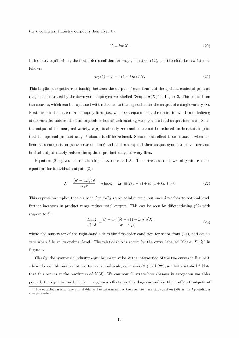
the k countries. Industry output is then given by:

Y = kmX. (20)

In industry equilibrium, the �rst-order condition for scope, equation (12), can therefore be rewritten as

follows:

w (�) = a0 � e (1 + km) b0X. (21)

This implies a negative relationship between the output of each �rm and the optimal choice of product

range, as illustrated by the downward-sloping curve labelled "Scope: � (X)" in Figure 3. This comes from

two sources, which can be explained with reference to the expression for the output of a single variety (8).

First, even in the case of a monopoly �rm (i.e., when km equals one), the desire to avoid cannibalizing

other varieties induces the �rm to produce less of each existing variety as its total output increases. Since

the output of the marginal variety, x (�), is already zero and so cannot be reduced further, this implies

that the optimal product range � should itself be reduced. Second, this e¤ect is accentuated when the

�rm faces competition (so km exceeds one) and all �rms expand their output symmetrically. Increases

in rival output clearly reduce the optimal product range of every �rm.

Equation (21) gives one relationship between � and X. To derive a second, we integrate over the

equations for individual outputs (8):

X =

�a0 � w�0

��

�1b0where: �1 � 2 (1� e) + e� (1 + km) > 0 (22)

This expression implies that a rise in � initially raises total output, but once � reaches its optimal level,

further increases in product range reduce total output. This can be seen by di¤erentiating (22) with

respect to � :d lnX

d ln �=a0 � w (�)� e (1 + km) b0X

a0 � w�0 (23)

where the numerator of the right-hand side is the �rst-order condition for scope from (21), and equals

zero when � is at its optimal level. The relationship is shown by the curve labelled "Scale: X (�)" in

Figure 3.

Clearly, the symmetric industry equilibrium must be at the intersection of the two curves in Figure 3,

where the equilibrium conditions for scope and scale, equations (21) and (22), are both satis�ed.8 Note

that this occurs at the maximum of X (�). We can now illustrate how changes in exogenous variables

perturb the equilibrium by considering their e¤ects on this diagram and on the pro�le of outputs of

8The equilibrium is unique and stable, as the determinant of the coe¢ cient matrix, equation (58) in the Appendix, isalways positive.

10

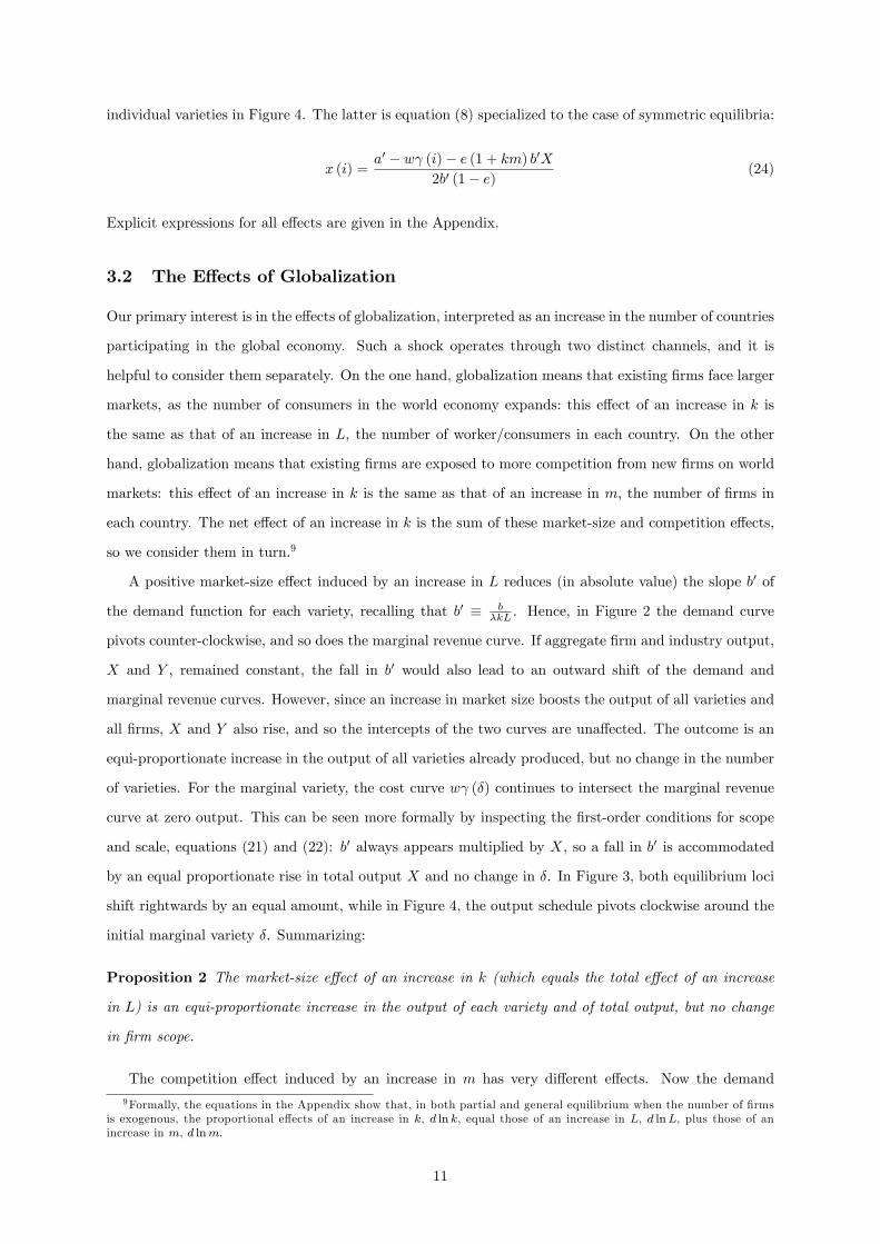
individual varieties in Figure 4. The latter is equation (8) specialized to the case of symmetric equilibria:

x (i) =a0 � w (i)� e (1 + km) b0X

2b0 (1� e) (24)

Explicit expressions for all e¤ects are given in the Appendix.

3.2 The E¤ects of Globalization

Our primary interest is in the e¤ects of globalization, interpreted as an increase in the number of countries

participating in the global economy. Such a shock operates through two distinct channels, and it is

helpful to consider them separately. On the one hand, globalization means that existing �rms face larger

markets, as the number of consumers in the world economy expands: this e¤ect of an increase in k is

the same as that of an increase in L, the number of worker/consumers in each country. On the other

hand, globalization means that existing �rms are exposed to more competition from new �rms on world

markets: this e¤ect of an increase in k is the same as that of an increase in m, the number of �rms in

each country. The net e¤ect of an increase in k is the sum of these market-size and competition e¤ects,

so we consider them in turn.9

A positive market-size e¤ect induced by an increase in L reduces (in absolute value) the slope b0 of

the demand function for each variety, recalling that b0 � b�kL . Hence, in Figure 2 the demand curve

pivots counter-clockwise, and so does the marginal revenue curve. If aggregate �rm and industry output,

X and Y , remained constant, the fall in b0 would also lead to an outward shift of the demand and

marginal revenue curves. However, since an increase in market size boosts the output of all varieties and

all �rms, X and Y also rise, and so the intercepts of the two curves are una¤ected. The outcome is an

equi-proportionate increase in the output of all varieties already produced, but no change in the number

of varieties. For the marginal variety, the cost curve w (�) continues to intersect the marginal revenue

curve at zero output. This can be seen more formally by inspecting the �rst-order conditions for scope

and scale, equations (21) and (22): b0 always appears multiplied by X, so a fall in b0 is accommodated

by an equal proportionate rise in total output X and no change in �. In Figure 3, both equilibrium loci

shift rightwards by an equal amount, while in Figure 4, the output schedule pivots clockwise around the

initial marginal variety �. Summarizing:

Proposition 2 The market-size e¤ect of an increase in k (which equals the total e¤ect of an increase

in L) is an equi-proportionate increase in the output of each variety and of total output, but no change

in �rm scope.

The competition e¤ect induced by an increase in m has very di¤erent e¤ects. Now the demand9Formally, the equations in the Appendix show that, in both partial and general equilibrium when the number of �rms

is exogenous, the proportional e¤ects of an increase in k, d ln k, equal those of an increase in L, d lnL, plus those of anincrease in m, d lnm.

11

curve intercept for every variety shifts downwards by the same absolute amount, while their slopes are

una¤ected. The output of every variety therefore falls by the same absolute amount, and so in Figure

4 the output pro�le shifts uniformly downwards. With output of every variety falling, total output X

must also fall.10 However, X falls less than proportionally to m, so industry output Y = kmX rises as a

result of the entry of new �rms: d lnYd lnm = 1+ d lnX

d lnm > 0. In addition, the uniform absolute fall in outputs

means that in relative terms greater competition hits harder those varieties produced at higher cost,

which implies that marginal varieties become unpro�table and so � falls. In Figure 3, both equilibrium

loci shift leftwards, but X (�) shifts by less.11 Summarizing:

Proposition 3 The competition e¤ect of an increase in k (which equals the total e¤ect of an increase

in m) is a uniform absolute fall in the output of each variety, coupled with falls in both total �rm output

and �rm scope, but a rise in industry output.

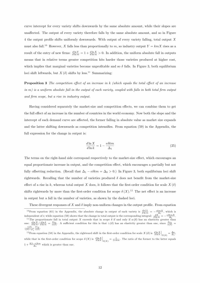
Having considered separately the market-size and competition e¤ects, we can combine them to get

the full e¤ect of an increase in the number of countries in the world economy. Now both the slope and the

intercept of each demand curve are a¤ected, the former falling in absolute value as market size expands

and the latter shifting downwards as competition intensi�es. From equation (59) in the Appendix, the

full expression for the change in output is:

d lnX

d ln k= 1� e�km

�1(25)

The terms on the right-hand side correspond respectively to the market-size e¤ect, which encourages an

equal proportionate increase in output, and the competition e¤ect, which encourages a partially but not

fully o¤setting reduction. (Recall that �1 � e�km = �0 > 0.) In Figure 3, both equilibrium loci shift

rightwards. Recalling that the number of varieties produced � does not bene�t from the market-size

e¤ect of a rise in k, whereas total output X does, it follows that the �rst-order condition for scale X (�)

shifts rightwards by more than the �rst-order condition for scope � (X).12 The net e¤ect is an increase

in output but a fall in the number of varieties, as shown by the dashed loci.

These divergent responses ofX and � imply non-uniform changes in the output pro�le. From equation

10From equation (61) in the Appendix, the absolute change in output of each variety is dx(i)d lnm

= � ekmX�1

, which is

independent of i; while equation (59) shows that the change in total output is the corresponding integral: dXd lnm

= � e�kmX�1

.11The proportionate fall in total output X exceeds that in scope � if and only if � (�) has an elasticity greater than

one: d lnXd lnm

= d ln �d lnm

= ����(�)

. A su¢ cient condition for this is that (�) has an elasticity greater than one, since ����(�)

=

(�) (�)��0

� � (�)

.

12From equation (58) in the Appendix, the rightward shift in the �rst-order condition for scale X (�) is d lnXd ln k

���X(�)

= �0�1;

while that in the �rst-order condition for scope � (X) is d lnXd ln k

����(X)

= 11+km

. The ratio of the former to the latter equals

1 +2(1�e)km

�1which is greater than one.

12

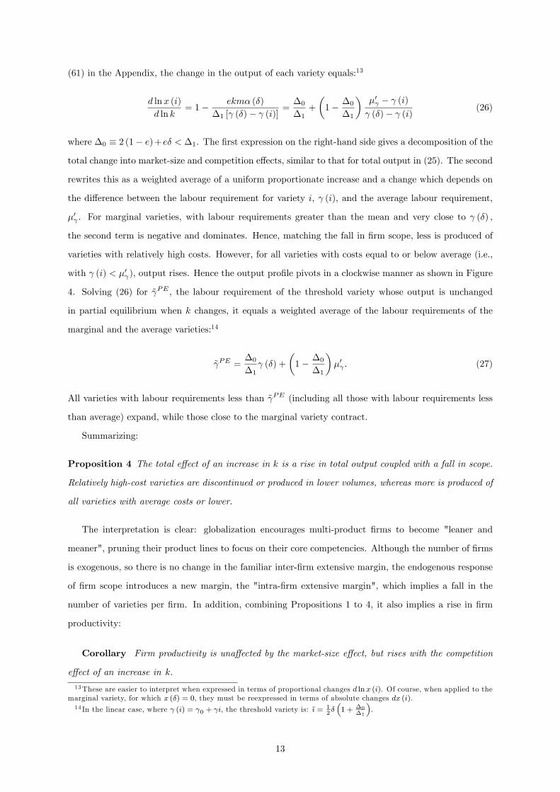
(61) in the Appendix, the change in the output of each variety equals:13

d lnx (i)

d ln k= 1� ekm� (�)

�1 [ (�)� (i)]=�0�1

+

�1� �0

�1

��0 � (i) (�)� (i) (26)

where �0 � 2 (1� e)+e� < �1. The �rst expression on the right-hand side gives a decomposition of the

total change into market-size and competition e¤ects, similar to that for total output in (25). The second

rewrites this as a weighted average of a uniform proportionate increase and a change which depends on

the di¤erence between the labour requirement for variety i, (i), and the average labour requirement,

�0 . For marginal varieties, with labour requirements greater than the mean and very close to (�) ;

the second term is negative and dominates. Hence, matching the fall in �rm scope, less is produced of

varieties with relatively high costs. However, for all varieties with costs equal to or below average (i.e.,

with (i) < �0 ), output rises. Hence the output pro�le pivots in a clockwise manner as shown in Figure

4. Solving (26) for ~ PE , the labour requirement of the threshold variety whose output is unchanged

in partial equilibrium when k changes, it equals a weighted average of the labour requirements of the

marginal and the average varieties:14

~ PE =�0�1 (�) +

�1� �0

�1

��0 : (27)

All varieties with labour requirements less than ~ PE (including all those with labour requirements less

than average) expand, while those close to the marginal variety contract.

Summarizing:

Proposition 4 The total e¤ect of an increase in k is a rise in total output coupled with a fall in scope.

Relatively high-cost varieties are discontinued or produced in lower volumes, whereas more is produced of

all varieties with average costs or lower.

The interpretation is clear: globalization encourages multi-product �rms to become "leaner and

meaner", pruning their product lines to focus on their core competencies. Although the number of �rms

is exogenous, so there is no change in the familiar inter-�rm extensive margin, the endogenous response

of �rm scope introduces a new margin, the "intra-�rm extensive margin", which implies a fall in the

number of varieties per �rm. In addition, combining Propositions 1 to 4, it also implies a rise in �rm

productivity:

Corollary Firm productivity is una¤ected by the market-size e¤ect, but rises with the competition

e¤ect of an increase in k.

13These are easier to interpret when expressed in terms of proportional changes d lnx (i). Of course, when applied to themarginal variety, for which x (�) = 0, they must be reexpressed in terms of absolute changes dx (i).14 In the linear case, where (i) = 0 + i, the threshold variety is: ~{ = 1

2��1 + �0

�1

�.

13

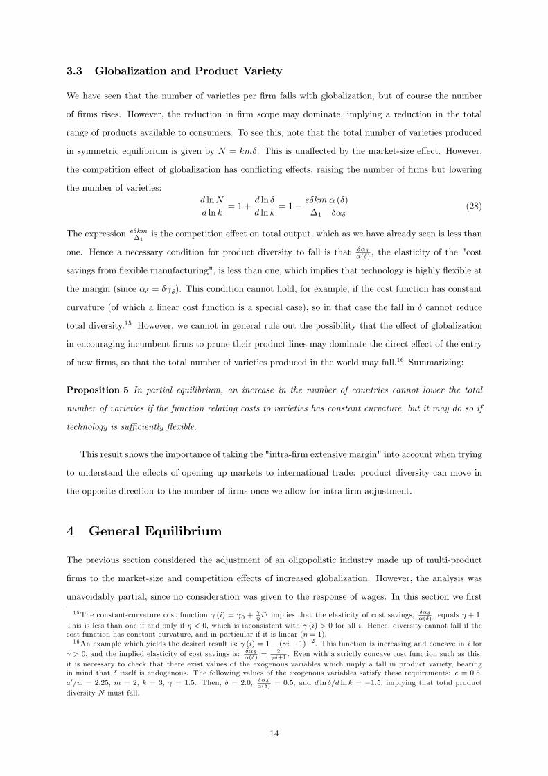
3.3 Globalization and Product Variety

We have seen that the number of varieties per �rm falls with globalization, but of course the number

of �rms rises. However, the reduction in �rm scope may dominate, implying a reduction in the total

range of products available to consumers. To see this, note that the total number of varieties produced

in symmetric equilibrium is given by N = km�. This is una¤ected by the market-size e¤ect. However,

the competition e¤ect of globalization has con�icting e¤ects, raising the number of �rms but lowering

the number of varieties:d lnN

d ln k= 1 +

d ln �

d ln k= 1� e�km

�1

� (�)

���(28)

The expression e�km�1

is the competition e¤ect on total output, which as we have already seen is less than

one. Hence a necessary condition for product diversity to fall is that ����(�) , the elasticity of the "cost

savings from �exible manufacturing", is less than one, which implies that technology is highly �exible at

the margin (since �� = � �). This condition cannot hold, for example, if the cost function has constant

curvature (of which a linear cost function is a special case), so in that case the fall in � cannot reduce

total diversity.15 However, we cannot in general rule out the possibility that the e¤ect of globalization

in encouraging incumbent �rms to prune their product lines may dominate the direct e¤ect of the entry

of new �rms, so that the total number of varieties produced in the world may fall.16 Summarizing:

Proposition 5 In partial equilibrium, an increase in the number of countries cannot lower the total

number of varieties if the function relating costs to varieties has constant curvature, but it may do so if

technology is su¢ ciently �exible.

This result shows the importance of taking the "intra-�rm extensive margin" into account when trying

to understand the e¤ects of opening up markets to international trade: product diversity can move in

the opposite direction to the number of �rms once we allow for intra-�rm adjustment.

4 General Equilibrium

The previous section considered the adjustment of an oligopolistic industry made up of multi-product

�rms to the market-size and competition e¤ects of increased globalization. However, the analysis was

unavoidably partial, since no consideration was given to the response of wages. In this section we �rst

15The constant-curvature cost function (i) = 0 + �i� implies that the elasticity of cost savings, ���

�(�), equals � + 1.

This is less than one if and only if � < 0, which is inconsistent with (i) > 0 for all i. Hence, diversity cannot fall if thecost function has constant curvature, and in particular if it is linear (� = 1).16An example which yields the desired result is: (i) = 1� ( i+ 1)�2. This function is increasing and concave in i for

> 0, and the implied elasticity of cost savings is: ����(�)

= 2 �+1

. Even with a strictly concave cost function such as this,it is necessary to check that there exist values of the exogenous variables which imply a fall in product variety, bearingin mind that � itself is endogenous. The following values of the exogenous variables satisfy these requirements: e = 0:5,a0=w = 2:25, m = 2, k = 3, = 1:5. Then, � = 2:0, ���

�(�)= 0:5, and d ln �=d ln k = �1:5, implying that total product

diversity N must fall.

14

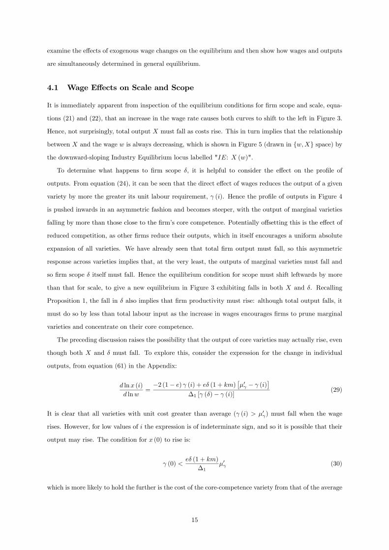
examine the e¤ects of exogenous wage changes on the equilibrium and then show how wages and outputs

are simultaneously determined in general equilibrium.

4.1 Wage E¤ects on Scale and Scope

It is immediately apparent from inspection of the equilibrium conditions for �rm scope and scale, equa-

tions (21) and (22), that an increase in the wage rate causes both curves to shift to the left in Figure 3.

Hence, not surprisingly, total output X must fall as costs rise. This in turn implies that the relationship

between X and the wage w is always decreasing, which is shown in Figure 5 (drawn in fw;Xg space) by

the downward-sloping Industry Equilibrium locus labelled "IE: X (w)".

To determine what happens to �rm scope �, it is helpful to consider the e¤ect on the pro�le of

outputs. From equation (24), it can be seen that the direct e¤ect of wages reduces the output of a given

variety by more the greater its unit labour requirement, (i). Hence the pro�le of outputs in Figure 4

is pushed inwards in an asymmetric fashion and becomes steeper, with the output of marginal varieties

falling by more than those close to the �rm�s core competence. Potentially o¤setting this is the e¤ect of

reduced competition, as other �rms reduce their outputs, which in itself encourages a uniform absolute

expansion of all varieties. We have already seen that total �rm output must fall, so this asymmetric

response across varieties implies that, at the very least, the outputs of marginal varieties must fall and

so �rm scope � itself must fall. Hence the equilibrium condition for scope must shift leftwards by more

than that for scale, to give a new equilibrium in Figure 3 exhibiting falls in both X and �. Recalling

Proposition 1, the fall in � also implies that �rm productivity must rise: although total output falls, it

must do so by less than total labour input as the increase in wages encourages �rms to prune marginal

varieties and concentrate on their core competence.

The preceding discussion raises the possibility that the output of core varieties may actually rise, even

though both X and � must fall. To explore this, consider the expression for the change in individual

outputs, from equation (61) in the Appendix:

d lnx (i)

d lnw=�2 (1� e) (i) + e� (1 + km)

��0 � (i)

��1 [ (�)� (i)]

(29)

It is clear that all varieties with unit cost greater than average ( (i) > �0 ) must fall when the wage

rises. However, for low values of i the expression is of indeterminate sign, and so it is possible that their

output may rise. The condition for x (0) to rise is:

(0) <e� (1 + km)

�1�0 (30)

which is more likely to hold the further is the cost of the core-competence variety from that of the average

15

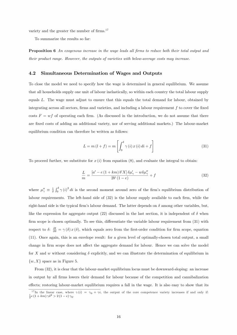
variety and the greater the number of �rms.17

To summarize the results so far:

Proposition 6 An exogenous increase in the wage leads all �rms to reduce both their total output and

their product range. However, the outputs of varieties with below-average costs may increase.

4.2 Simultaneous Determination of Wages and Outputs

To close the model we need to specify how the wage is determined in general equilibrium. We assume

that all households supply one unit of labour inelastically, so within each country the total labour supply

equals L. The wage must adjust to ensure that this equals the total demand for labour, obtained by

integrating across all sectors, �rms and varieties, and including a labour requirement f to cover the �xed

costs F = wf of operating each �rm. (As discussed in the introduction, we do not assume that there

are �xed costs of adding an additional variety, nor of serving additional markets.) The labour-market

equilibrium condition can therefore be written as follows:

L = m (l + f) = m

"Z �

0

(i)x (i) di+ f

#(31)

To proceed further, we substitute for x (i) from equation (8), and evaluate the integral to obtain:

L

m=[a0 � e (1 + km) b0X] ��0 � w��00

2b0 (1� e) + f (32)

where �00 � 1�

R �0 (i)

2di is the second moment around zero of the �rm�s equilibrium distribution of

labour requirements. The left-hand side of (32) is the labour supply available to each �rm, while the

right-hand side is the typical �rm�s labour demand. The latter depends on � among other variables, but,

like the expression for aggregate output (22) discussed in the last section, it is independent of � when

�rm scope is chosen optimally. To see this, di¤erentiate the variable labour requirement from (31) with

respect to �: @l@� = (�)x (�), which equals zero from the �rst-order condition for �rm scope, equation

(11). Once again, this is an envelope result: for a given level of optimally-chosen total output, a small

change in �rm scope does not a¤ect the aggregate demand for labour. Hence we can solve the model

for X and w without considering � explicitly, and we can illustrate the determination of equilibrium in

fw;Xg space as in Figure 5.

From (32), it is clear that the labour-market equilibrium locus must be downward-sloping: an increase

in output by all �rms lowers their demand for labour because of the competition and cannibalization

e¤ects; restoring labour-market equilibrium requires a fall in the wage. It is also easy to show that its

17 In the linear case, where (i) = 0 + i, the output of the core competence variety increases if and only if:12e (1 + km) �2 > 2 (1� e) 0.

16

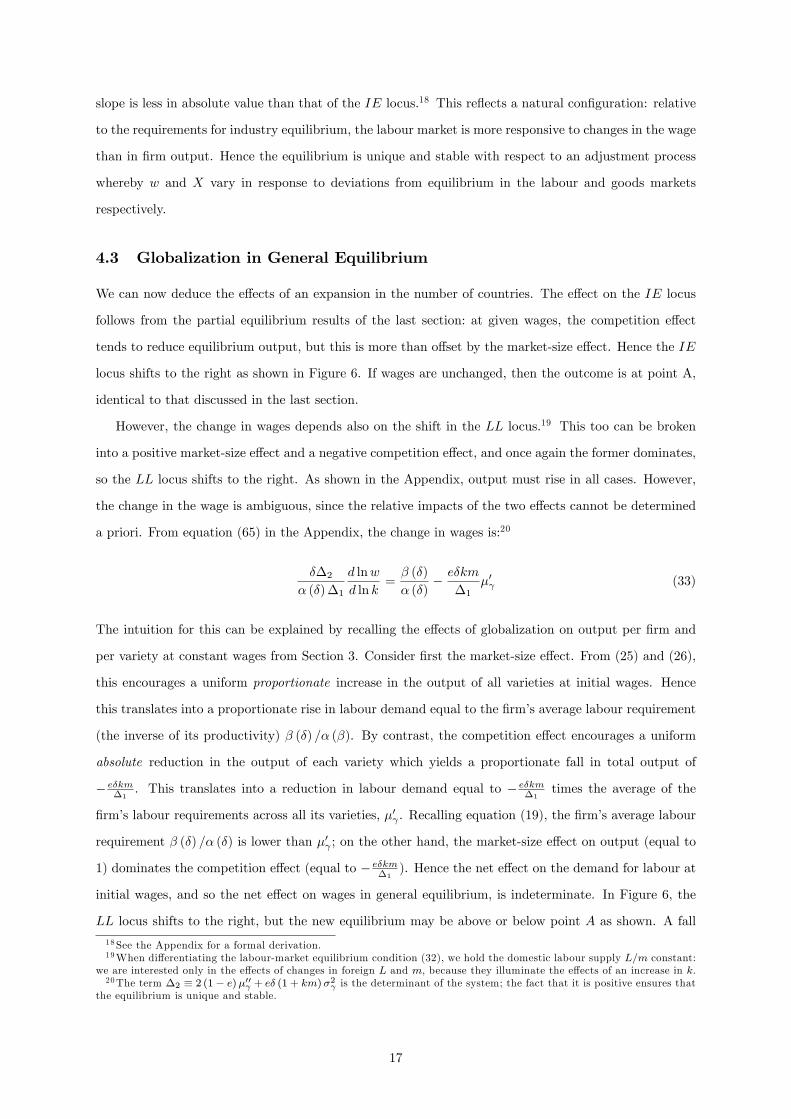
slope is less in absolute value than that of the IE locus.18 This re�ects a natural con�guration: relative

to the requirements for industry equilibrium, the labour market is more responsive to changes in the wage

than in �rm output. Hence the equilibrium is unique and stable with respect to an adjustment process

whereby w and X vary in response to deviations from equilibrium in the labour and goods markets

respectively.

4.3 Globalization in General Equilibrium

We can now deduce the e¤ects of an expansion in the number of countries. The e¤ect on the IE locus

follows from the partial equilibrium results of the last section: at given wages, the competition e¤ect

tends to reduce equilibrium output, but this is more than o¤set by the market-size e¤ect. Hence the IE

locus shifts to the right as shown in Figure 6. If wages are unchanged, then the outcome is at point A,

identical to that discussed in the last section.

However, the change in wages depends also on the shift in the LL locus.19 This too can be broken

into a positive market-size e¤ect and a negative competition e¤ect, and once again the former dominates,

so the LL locus shifts to the right. As shown in the Appendix, output must rise in all cases. However,

the change in the wage is ambiguous, since the relative impacts of the two e¤ects cannot be determined

a priori. From equation (65) in the Appendix, the change in wages is:20

��2� (�)�1

d lnw

d ln k=� (�)

� (�)� e�km

�1�0 (33)

The intuition for this can be explained by recalling the e¤ects of globalization on output per �rm and

per variety at constant wages from Section 3. Consider �rst the market-size e¤ect. From (25) and (26),

this encourages a uniform proportionate increase in the output of all varieties at initial wages. Hence

this translates into a proportionate rise in labour demand equal to the �rm�s average labour requirement

(the inverse of its productivity) � (�) =� (�). By contrast, the competition e¤ect encourages a uniform

absolute reduction in the output of each variety which yields a proportionate fall in total output of

� e�km�1

. This translates into a reduction in labour demand equal to � e�km�1

times the average of the

�rm�s labour requirements across all its varieties, �0 . Recalling equation (19), the �rm�s average labour

requirement � (�) =� (�) is lower than �0 ; on the other hand, the market-size e¤ect on output (equal to

1) dominates the competition e¤ect (equal to � e�km�1

). Hence the net e¤ect on the demand for labour at

initial wages, and so the net e¤ect on wages in general equilibrium, is indeterminate. In Figure 6, the

LL locus shifts to the right, but the new equilibrium may be above or below point A as shown. A fall

18See the Appendix for a formal derivation.19When di¤erentiating the labour-market equilibrium condition (32), we hold the domestic labour supply L=m constant:

we are interested only in the e¤ects of changes in foreign L and m, because they illuminate the e¤ects of an increase in k.20The term �2 � 2 (1� e)�00 + e� (1 + km)�2 is the determinant of the system; the fact that it is positive ensures that

the equilibrium is unique and stable.

17

in wages, implying a new equilibrium such as that at A0, reinforces the increase in total output that we

saw in partial equilibrium. However, a rise in wages leading to a point such as A00 o¤sets it, though it

cannot do so fully as we have seen.

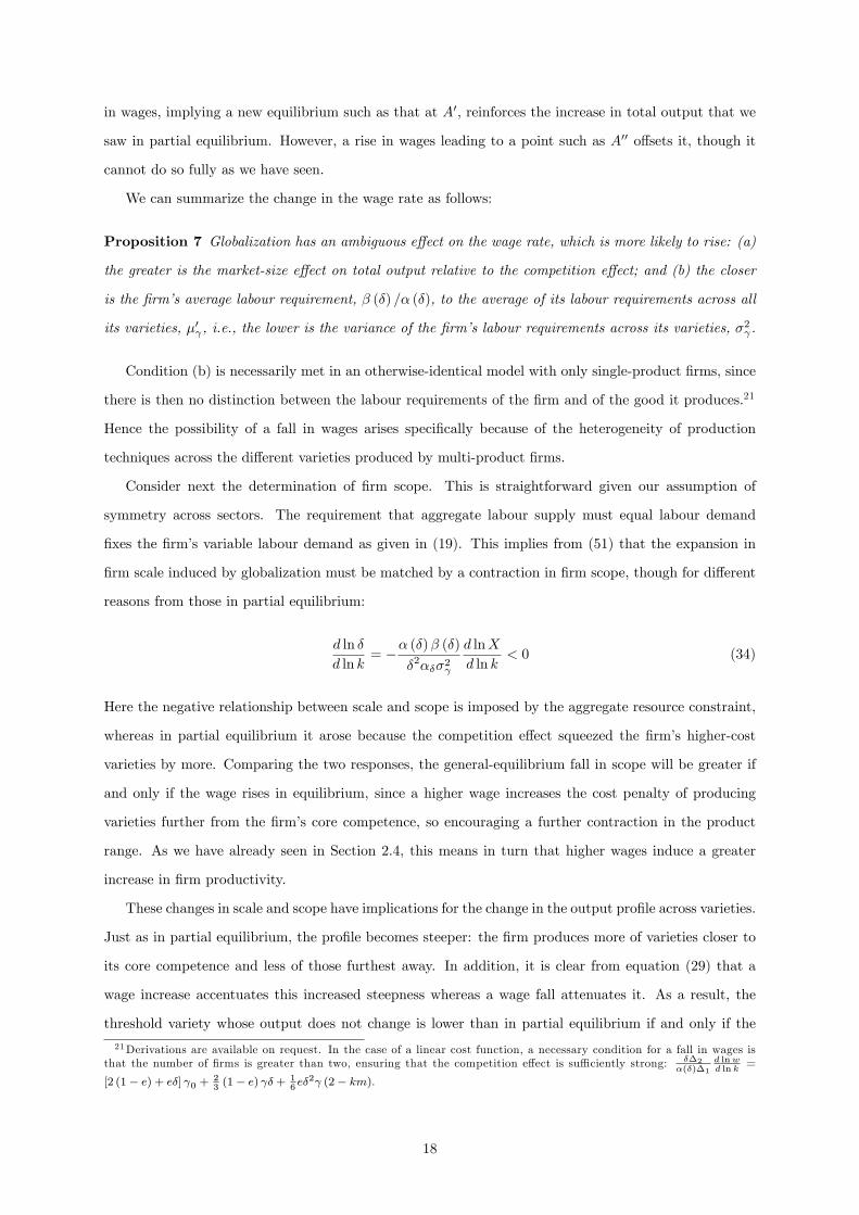
We can summarize the change in the wage rate as follows:

Proposition 7 Globalization has an ambiguous e¤ect on the wage rate, which is more likely to rise: (a)

the greater is the market-size e¤ect on total output relative to the competition e¤ect; and (b) the closer

is the �rm�s average labour requirement, � (�) =� (�), to the average of its labour requirements across all

its varieties, �0 , i.e., the lower is the variance of the �rm�s labour requirements across its varieties, �2 .

Condition (b) is necessarily met in an otherwise-identical model with only single-product �rms, since

there is then no distinction between the labour requirements of the �rm and of the good it produces.21

Hence the possibility of a fall in wages arises speci�cally because of the heterogeneity of production

techniques across the di¤erent varieties produced by multi-product �rms.

Consider next the determination of �rm scope. This is straightforward given our assumption of

symmetry across sectors. The requirement that aggregate labour supply must equal labour demand

�xes the �rm�s variable labour demand as given in (19). This implies from (51) that the expansion in

�rm scale induced by globalization must be matched by a contraction in �rm scope, though for di¤erent

reasons from those in partial equilibrium:

d ln �

d ln k= �� (�)� (�)

�2���2

d lnX

d ln k< 0 (34)

Here the negative relationship between scale and scope is imposed by the aggregate resource constraint,

whereas in partial equilibrium it arose because the competition e¤ect squeezed the �rm�s higher-cost

varieties by more. Comparing the two responses, the general-equilibrium fall in scope will be greater if

and only if the wage rises in equilibrium, since a higher wage increases the cost penalty of producing

varieties further from the �rm�s core competence, so encouraging a further contraction in the product

range. As we have already seen in Section 2.4, this means in turn that higher wages induce a greater

increase in �rm productivity.

These changes in scale and scope have implications for the change in the output pro�le across varieties.

Just as in partial equilibrium, the pro�le becomes steeper: the �rm produces more of varieties closer to

its core competence and less of those furthest away. In addition, it is clear from equation (29) that a

wage increase accentuates this increased steepness whereas a wage fall attenuates it. As a result, the

threshold variety whose output does not change is lower than in partial equilibrium if and only if the

21Derivations are available on request. In the case of a linear cost function, a necessary condition for a fall in wages isthat the number of �rms is greater than two, ensuring that the competition e¤ect is su¢ ciently strong: ��2

�(�)�1

d lnwd ln k

=

[2 (1� e) + e�] 0 +23(1� e) � + 1

6e�2 (2� km).

18

wage rises:

~ PE � ~ GE = � (�)

��0

�� (�)

� (�)� e�km

�1�0

�=

�2�0 �1

d lnw

d ln k(35)

(See the Appendix for an explicit proof.) This implies that a higher wage induces the �rm to reduce the

output of more products, so increasing the tendency towards a leaner output pro�le.

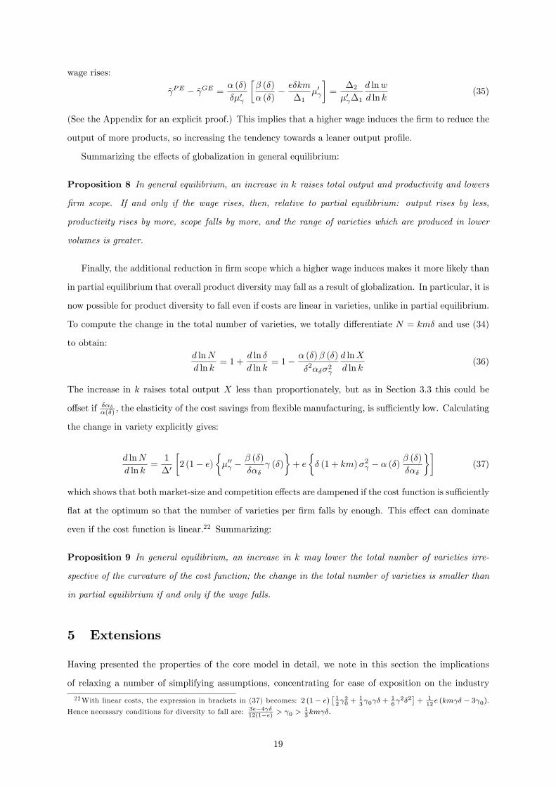
Summarizing the e¤ects of globalization in general equilibrium:

Proposition 8 In general equilibrium, an increase in k raises total output and productivity and lowers

�rm scope. If and only if the wage rises, then, relative to partial equilibrium: output rises by less,

productivity rises by more, scope falls by more, and the range of varieties which are produced in lower

volumes is greater.

Finally, the additional reduction in �rm scope which a higher wage induces makes it more likely than

in partial equilibrium that overall product diversity may fall as a result of globalization. In particular, it is

now possible for product diversity to fall even if costs are linear in varieties, unlike in partial equilibrium.

To compute the change in the total number of varieties, we totally di¤erentiate N = km� and use (34)

to obtain:d lnN

d ln k= 1 +

d ln �

d ln k= 1� � (�)� (�)

�2���2

d lnX

d ln k(36)

The increase in k raises total output X less than proportionately, but as in Section 3.3 this could be

o¤set if ����(�) , the elasticity of the cost savings from �exible manufacturing, is su¢ ciently low. Calculating

the change in variety explicitly gives:

d lnN

d ln k=1

�0

�2 (1� e)

��00 �

� (�)

��� (�)

�+ e

�� (1 + km)�2 � � (�)

� (�)

���

��(37)

which shows that both market-size and competition e¤ects are dampened if the cost function is su¢ ciently

�at at the optimum so that the number of varieties per �rm falls by enough. This e¤ect can dominate

even if the cost function is linear.22 Summarizing:

Proposition 9 In general equilibrium, an increase in k may lower the total number of varieties irre-

spective of the curvature of the cost function; the change in the total number of varieties is smaller than

in partial equilibrium if and only if the wage falls.

5 Extensions

Having presented the properties of the core model in detail, we note in this section the implications

of relaxing a number of simplifying assumptions, concentrating for ease of exposition on the industry

22With linear costs, the expression in brackets in (37) becomes: 2 (1� e)�12 20 +

13 0 � +

16 2�2

�+ 1

12e (km � � 3 0).

Hence necessary conditions for diversity to fall are: 3e�4 �12(1�e) > 0 >

13km �.

19

equilibrium case. The working paper version of our paper, Eckel and Neary (2005), shows that the results

are also robust to relaxing the assumption of symmetry, allowing for both inter-country asymmetries and

for the coexistence of single- and multi-product �rms.

5.1 Free Entry

The assumption of free entry sits uneasily with our model in which �rms produce a large portfolio of

di¤erentiated varieties and engage in strategic interaction with each other.23 Nevertheless it is desirable

to check that our results are robust to relaxing the assumption that the number of �rms in each country

is �xed. This implies adding a third margin of adjustment, the "inter-�rm extensive margin", to our

model which so far has concentrated on the intensive margin and the "intra-�rm extensive margin".

We therefore reexamine the e¤ects of globalization treating the number of �rms per country, m, as a

continuous variable.

To establish the e¤ects of globalization on the incentives for entry or exit, we �rst consider its e¤ects

on pro�ts for a given number of �rms. Substituting from the �rst-order conditions for output (7) into

expression (6) for pro�ts, we �nd that operating pro�ts � are proportional to a weighted average of the

square of total output and the integral of squared outputs of all varieties:

� = � � F where: � = b0

"(1� e)

Z �

0

x (i)2di+ eX2

#(38)

To help with intuition in what follows, note that, for a given level of total output X, pro�ts are greater

the larger is the ratio ofR �0x (i)

2di to X2. As we show in the Appendix, this ratio can be interpreted as

an index of the �exibility of technology, which we denote by � �R �0x (i)

2di=X2: high values of � imply

that there is a relatively large variance in the cost savings on infra-marginal varieties due to �exible

manufacturing.

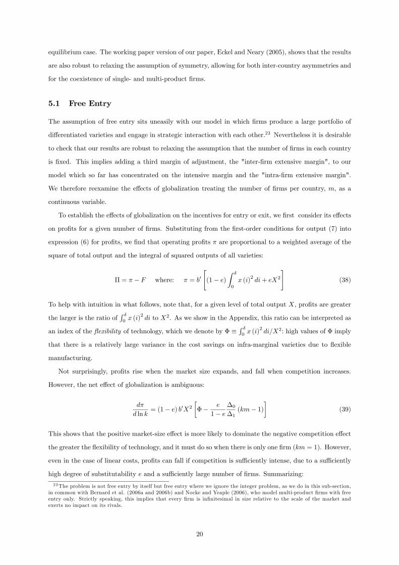
Not surprisingly, pro�ts rise when the market size expands, and fall when competition increases.

However, the net e¤ect of globalization is ambiguous:

d�

d ln k= (1� e) b0X2

��� e

1� e�0�1

(km� 1)�

(39)

This shows that the positive market-size e¤ect is more likely to dominate the negative competition e¤ect

the greater the �exibility of technology, and it must do so when there is only one �rm (km = 1). However,

even in the case of linear costs, pro�ts can fall if competition is su¢ ciently intense, due to a su¢ ciently

high degree of substitutability e and a su¢ ciently large number of �rms. Summarizing:

23The problem is not free entry by itself but free entry where we ignore the integer problem, as we do in this sub-section,in common with Bernard et al. (2006a and 2006b) and Nocke and Yeaple (2006), who model multi-product �rms with freeentry only. Strictly speaking, this implies that every �rm is in�nitesimal in size relative to the scale of the market andexerts no impact on its rivals.

20

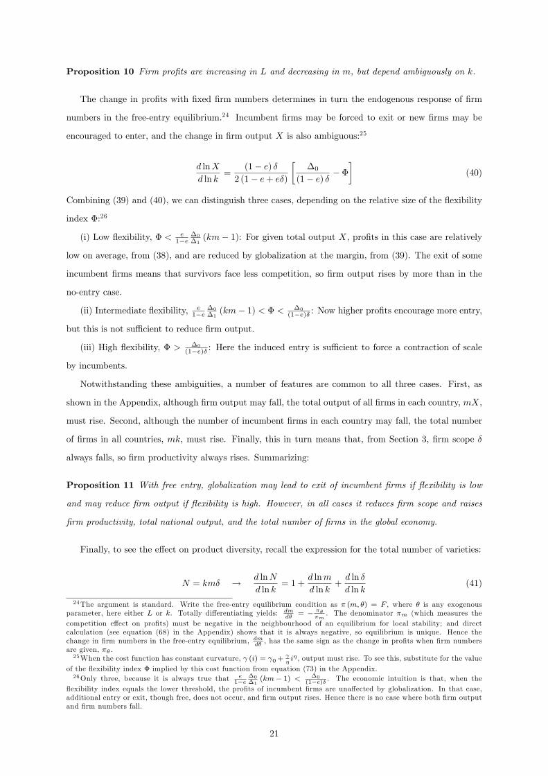
Proposition 10 Firm pro�ts are increasing in L and decreasing in m, but depend ambiguously on k.

The change in pro�ts with �xed �rm numbers determines in turn the endogenous response of �rm

numbers in the free-entry equilibrium.24 Incumbent �rms may be forced to exit or new �rms may be

encouraged to enter, and the change in �rm output X is also ambiguous:25

d lnX

d ln k=

(1� e) �2 (1� e+ e�)

��0

(1� e) � � ��

(40)

Combining (39) and (40), we can distinguish three cases, depending on the relative size of the �exibility

index �:26

(i) Low �exibility, � < e1�e

�0

�1(km� 1): For given total output X, pro�ts in this case are relatively

low on average, from (38), and are reduced by globalization at the margin, from (39). The exit of some

incumbent �rms means that survivors face less competition, so �rm output rises by more than in the

no-entry case.

(ii) Intermediate �exibility, e1�e

�0

�1(km� 1) < � < �0

(1�e)� : Now higher pro�ts encourage more entry,

but this is not su¢ cient to reduce �rm output.

(iii) High �exibility, � > �0

(1�e)� : Here the induced entry is su¢ cient to force a contraction of scale

by incumbents.

Notwithstanding these ambiguities, a number of features are common to all three cases. First, as

shown in the Appendix, although �rm output may fall, the total output of all �rms in each country, mX,

must rise. Second, although the number of incumbent �rms in each country may fall, the total number

of �rms in all countries, mk, must rise. Finally, this in turn means that, from Section 3, �rm scope �

always falls, so �rm productivity always rises. Summarizing:

Proposition 11 With free entry, globalization may lead to exit of incumbent �rms if �exibility is low

and may reduce �rm output if �exibility is high. However, in all cases it reduces �rm scope and raises

�rm productivity, total national output, and the total number of �rms in the global economy.

Finally, to see the e¤ect on product diversity, recall the expression for the total number of varieties:

N = km� ! d lnN

d ln k= 1 +

d lnm

d ln k+d ln �

d ln k(41)

24The argument is standard. Write the free-entry equilibrium condition as � (m; �) = F , where � is any exogenousparameter, here either L or k. Totally di¤erentiating yields: dm

d�= � ��

�m. The denominator �m (which measures the

competition e¤ect on pro�ts) must be negative in the neighbourhood of an equilibrium for local stability; and directcalculation (see equation (68) in the Appendix) shows that it is always negative, so equilibrium is unique. Hence thechange in �rm numbers in the free-entry equilibrium, dm

d�, has the same sign as the change in pro�ts when �rm numbers

are given, �� .25When the cost function has constant curvature, (i) = 0+

�i� , output must rise. To see this, substitute for the value

of the �exibility index � implied by this cost function from equation (73) in the Appendix.26Only three, because it is always true that e

1�e�0�1

(km� 1) < �0(1�e)� . The economic intuition is that, when the

�exibility index equals the lower threshold, the pro�ts of incumbent �rms are una¤ected by globalization. In that case,additional entry or exit, though free, does not occur, and �rm output rises. Hence there is no case where both �rm outputand �rm numbers fall.

21

In the free-entry case, the total change in � can be decomposed into the impact e¤ect of globalization

without entry (i.e.,the e¤ect considered in Section 3) and the induced e¤ect of the rise in the number of

�rms per country:d ln �

d ln k=@ ln �

@ ln k+@ ln �

@ lnm

d lnm

d ln k=@ ln �

@ ln k

�1 +

d lnm

d ln k

�(42)

The second equality follows because, as we saw in Section 3, there is no market-size e¤ect on product

scope, so the partial e¤ects @ ln �@ ln k and

@ ln �@ lnm are the same. Hence the total change in product diversity

from (41) can be written as:d lnN

d ln k=

�1 +

@ ln �

@ ln k

��1 +

d lnm

d ln k

�(43)

The �rst expression in brackets is the total change in N without entry: as we saw in Section 3, this can

be negative if technology is su¢ ciently �exible at the optimal variety. The second expression in brackets

is the total increase in the number of �rms in the world market following a unit increase in k: as we have

seen in Proposition 11 this can be greater or less than one but must be positive. Hence we can conclude

that the e¤ect on diversity of changes in the inter-�rm extensive margin induced by globalization cannot

reverse the e¤ect of changes in the intra-�rm extensive margin. The total e¤ect is qualitatively the same

as in the no-entry case. Summarizing these results:

Proposition 12 With free entry, the e¤ect of globalization on total product variety is qualitatively iden-

tical to that in the no-entry case, but may be greater or less in absolute value.

With appropriate quali�cations therefore, the e¤ects of globalization when entry is free are qualita-

tively the same as those in the no-entry case already considered.27

5.2 Heterogeneous Firms

Our presentation of the core model assumed for simplicity that �rms were identical, but it is straightfor-

ward to show that the main results continue to hold when this assumption is relaxed. Returning to the

case of no entry, we assume a given con�guration of �rms with arbitrary di¤erences in their cost schedules

j (i), subject to the boundary constraint that all produce at least some varieties in equilibrium.

Substituting (18) into (20) yields a single expression for industry output:

Y =mPj=1

Xj where: Xj =w�j (�j)

2b0 (1� e) , (44)

Clearly, industry output is increasing in the product range of every multi-product �rm. Similarly,

substituting (18) into (12) yields an expression for the product range of each multi-product �rm as

27For ease of exposition this sub-section has presented results for the case of free entry in partial equilibrium only.Qualitatively identical results for changes in X, m and � hold in general equilibrium: details on request.

22

a function of industry output:

w j (�j) +e

2 (1� e)w�j (�j) = a0 � b0eY (45)

Equations (44) and (45) comprise m + 1 equations in �j and Y that can be solved for the industry

equilibrium, with each �rm�s total output recoverable from (44). It is straightforward to show that the

responses of each �rm to changes in L, m and k are qualitatively identical to the average responses

derived in Section 3.28 (Details are available on request.) In addition, we can compare the responses

of di¤erent multi-product �rms. The relative responses of the product ranges of any two multi-product

�rms j and h to changes in L or k are given by:

d�jd�h

='j�j'h�h

(46)

where:

'j �(2� e) �j

2 (1� e) + e�jand �j �

h�jc

j� (�j)

i�1(47)

Here 'j is an increasing concave function of the product range �j , while �j is the inverse semi-elasticity

of marginal cost, evaluated at the marginal variety, and so can be interpreted as a local measure of �rm

j�s marginal �exibility of production (by contrast with the global measure � used in the last sub-section).

Equation (46) shows that �rms with longer product lines (for a given marginal �exibility) and with more

�exible technology at the margin (for a given length of product line) tend to respond more to shocks.

The former result is consistent with the empirical �nding of Bernard, Redding and Schott (2006) that

larger �rms are more active in changing their product mix.

These results can be summarized as follows:

Proposition 13 In partial equilibrium, an increase in competition reduces the product range �j of all

multi-product �rms and raises industry output Y . An increase in the size of the market also leads to

an increase in industry output Y but leaves the product ranges �j una¤ected. Multi-product �rms with

longer product lines and with more �exible technology tend to respond more to changes in market size

and in the number of countries in the global economy.

5.3 Partial Trade Liberalization

So far we have modelled the process of globalization as an all-or-nothing one, with previously autarkic

economies joining a free-trading world. A natural question to ask is how the results are a¤ected when

we consider instead the more realistic case of a partial reduction of pre-existing non-prohibitive trade

28When �rms are heterogeneous, we cannot simply di¤erentiate with respect to m. However, inspection of equations(44) and (45) con�rms that (provided all incumbent �rms remain pro�table) the entry of an additional �rm in any countryhas a competition e¤ect on incumbent �rms with the same qualitative properties as in the homogeneous-�rms case.

23

barriers. Exploring this extension in detail would take us too far a�eld, but it su¢ ces to note brie�y

that the qualitative results of the paper continue to hold, subject to two quali�cations.

The �rst quali�cation, familiar since Brander (1981), is that the relative importance of the competition

and market-size e¤ects di¤ers depending on the initial height of trade costs. Suppose that the home and

foreign markets are segmented, and that foreign sales incur speci�c tari¤s. (Transport costs would have

similar relative-price e¤ects.) Hence the competition and market-size e¤ects apply to home and foreign

sales respectively. When the initial tari¤ is prohibitive, a small multilateral reduction in tari¤s exposes

domestic sales to a �nite competition e¤ect (since pro�t margins are squeezed on all units sold) whereas

exports bene�t from only an in�nitesimal market-size e¤ect (since exports are initially zero). Hence the

negative competition e¤ect dominates, so both �rm scale and scope should contract, and pro�ts fall,

encouraging exit of some incumbent �rms. By contrast, starting from free trade, the imposition of a

small tari¤ bene�ts home sales by a small competition e¤ect (since rivals�costs rise) but imposes a larger

negative market-size e¤ect on export sales (since the �rm�s own costs of serving foreign customers rise).

Hence in this case too the negative e¤ect dominates, now encouraging a fall in output though possibly

a rise in scope, coupled with a fall in pro�ts. The e¤ects derived in the main body of the paper are the

integral of the combined e¤ects as trade costs are progressively lowered.

A second quali�cation arises from the special character of our model of multi�product �rms. Not

only the volume of sales but also the range of products sold will di¤er in general between markets. With

obvious extensions, the model predicts that �rms will sell a larger range of products in markets that

have lower access costs and fewer competitors; while the volume of sales will be increasing in the size

of the market, holding tari¤s and numbers of competitors constant. For high trade costs only products

close to a �rm�s core competence will be exported, while trade liberalization is likely to encourage �rms

to expand the range of products exported. Re�ning these predictions and confronting them with data is

an obvious priority for future work.

6 Conclusion

In this paper we have developed a new model of multi-product �rms which highlights the role of �exible

manufacturing. In line with the increasing empirical evidence that adjustments in the range of products

produced by �rms are an important component of changes in output and exports, our model highlights

this hitherto-neglected channel of adjustment. Our focus is on the intra-�rm adjustments within multi-

product �rms and we �nd that economy-wide shocks can have a considerable impact on both scale and

scope. In addition, our analysis shows that the general-equilibrium feedback e¤ects, through changes in

wages and income, are an important determinant of changes in product ranges.

Two predictions of our model stand out. First, the model highlights a new source of gains from

24

trade, as within-�rm adjustments generate a rise in productivity, even in the absence of entry and

exit. Existing �rms face pressure to become "leaner and meaner", contracting their product range in

response to additional competition, while simultaneously expanding total output to avail of new foreign

markets. Hence selection e¤ects operate at the product level, with �rms encouraged to focus on their

"core competence" and drop marginal high-cost varieties. Second, the model draws attention to a new

source of potential losses from trade liberalization, in the form of a fall in product diversity. Even though

the number of �rms in the global economy rises, each produces fewer products, and the latter e¤ect may

dominate if technology is su¢ ciently �exible.

Our results suggest that adjustment processes within multi-product �rms are signi�cantly di¤erent

from adjustments through exit and entry. Standard trade theory based on single-product �rms in monop-

olistic competition predicts that international market integration raises the real wages of all participating

countries and unambiguously increases the choices available to consumers. While this outcome is still

possible in our framework, our results show that other outcomes are also possible depending on the ex-

tent of competition and on the degree of �exibility in manufacturing. First, the change in the real wage

depends on whether the impact of an increase in competition from abroad is accompanied by an increase

in foreign demand, because the competition e¤ect tends to lower the real wage while the demand e¤ect

tends to raise it. Second, if manufacturing technologies are highly �exible, multi-product �rms respond

to shocks more by altering their product range than their total output, which can lead to a fall in overall

product diversity when new countries enter the world market.29 These results are substantially di¤erent

from the predictions of standard trade theory even though both sets of results are driven by the same

forces, an increase in the number of �rms and an increase in the size of the market. This di¤erence in

predictions underlines the importance of adjustments on the intra-�rm extensive margin which our model

highlights. At the same time, Section 5.1 shows that our model�s predictions are robust to allowing for

�rm entry and exit, which adds adjustment on the inter-�rm extensive margin, familiar from standard

models of monopolistic competition, to the intra-�rm adjustments of our model.

Furthermore, our look inside a �rm�s product range reveals new and testable insights into how infra-

marginal products adjust. Because �exible manufacturing creates cost heterogeneities within �rms,

asymmetric adjustment processes are possible that di¤er signi�cantly from adjustments via exit and

entry. These processes arise even at the level of a single industry, and they are accentuated by changes

in factor prices, underlining the importance of a general equilibrium approach.

Our framework can be extended in various directions. In Eckel and Neary (2006) we present an

extension that analyzes the general-equilibrium feedback e¤ects between asymmetric industries. This

provides insights into how adjustments within multi-product �rms can di¤er between industries and

29This is quite consistent with the �ndings of Broda and Weinstein (2006) that the diversity of imports has increased asa result of trade liberalization. Moreover, their study assumes CES preferences, which place a higher premium on diversitythan quadratic preferences.

25

shows that industries which are not subject to direct foreign competition in their own markets are still

a¤ected by a competition e¤ect through the labor market. We also allow for heterogeneous �rms in our

partial equilibrium analysis. Further extensions, to allow for heterogeneous �rms in general equilibrium,

and to consider how �rms choose their degree of �exibility, seem well worth exploring in our framework.

Empirical evidence suggests that multi-product �rms are an important feature of modern industries.

Our results show that adjustment processes within multi-product �rms di¤er substantially from adjust-

ments via exit and entry and that globalization can be a driving force of these adjustment processes.

26

7 Appendix

7.1 Preliminaries

Equations (16) and (18) introduced shorthand terms � (�) and � (�) for the technological components

of the integrals of labour demand and output respectively, while equations (19) and (32) introduced the

�rst and second central moments and the variance of the distribution of labour requirements across all

the varieties produced by each �rm in equilibrium. These terms can be related to each other as follows:

� (�) = �� (�)� �0

�(48)

� (�) = �� (�)�0 � �00

�= � (�)�0 � ��2 =

� (�)�00 � � (�)�2 �0

(49)

Similarly for their derivatives:

�� = � � �� = �0 �� (50)

7.2 Changes in Productivity: Proof of Proposition 1

Consider �rst the change in productivity when output changes are uniformly weighted. Using the ex-

pressions for � (�), �� and �� from (49) and (50), the logarithmic change in measured productivity with

respect to a change in �rm scope is given by:

@ lnLP

@ ln �

����h(i)=1

=@ lnX

@ ln �� @ ln l

@ ln �=d ln� (�)

d ln �� d ln� (�)

d ln �=���� (�)

� ���� (�)

= ��2���

2

� (�)� (�)(51)

Since the variance �2 must be positive, it follows that productivity is decreasing in � as claimed.

Consider next the change in productivity when output changes are price-weighted:

@ lnLP

@ ln �

����h(i)=p(i)

=

R �0p (i) @x(i)@ ln � diR �

0p (i)x (i) di

� @ ln l

@ ln �(52)

As we have already seen, the change in labour input is: @ ln l@ ln � =����(�) = �

�0 ���(�) . Turning to the change in

output, we �rst write the value of output of a single variety as a function of its own and the threshold

variety�s unit labour requirements:

p (i)x (i) = w

�1

2f (i) + (�)g+ e � (�)

2 (1� e)

�w

2 (1� e) b0 [ (�)� (i)] (53)

Integrating over all varieties produced by the �rm and simplifying yields:

Z �

0

p (i)x (i) di =w2

4 (1� e)2 b0H where: H � (1� e) f� (�) (�) + � (�)g+ e� (�)2 (54)

27

Similarly, the numerator of the weighted output change can be written as:

Z �

0

p (i)@x (i)

@ ln �di =

w2

4 (1� e)2 b0�(1� e)

��0 + (�)

+ e� (�)

���� (55)

Combining these results, we see that:

@ lnLP

@ ln �

����h(i)=p(i)

=(1� e)

��0 + (�)

+ e� (�)

H��� � �

�0 ��

� (�)(56)

Simplifying, this becomes:

@ lnLP

@ ln �

����h(i)=p(i)

= � �2��� (�)H

[(1� e) (�) + e� (�)]�2 < 0 (57)

This is negative, but, as can easily be checked, it is less so than the change in the �xed-weight productivity

index given in (51), which con�rms the results stated in Proposition 1.

7.3 Industry Equilibrium: Comparative Statics

Totally di¤erentiating the equilibrium conditions for scope and scale, equations (21) and (22), with the

results written as a matrix equation, gives:

264 �1 0

e (1 + km) 2(1�e)� ��(�)

375264 d lnX

d ln �

375 =264 �1

e (1 + km)

375 d lnL (58)

�

264 �

1

375 ekmd lnm+264 �0

e

375 d ln k �264 ��0

(�)

375 2 (1� e)� (�)

d lnw

where �1 and �0 are de�ned in (22) and (26), with �1 > �0 > 0. The solutions are as follows:

d lnX = d lnL� e�km�1

d lnm+�0�1d ln k �

2 (1� e) ��0 �1� (�)

d lnw (59)

and

d ln � = �e�km� (�)�1���

(d lnm+ d ln k)�2 (1� e) ��0 +�1� (�)

�1���d lnw (60)

Note that d lnXd lnm = �

�1� �0

�1

�> �1, so d lnY

d lnm = 1� d lnXd lnm > 0 as noted in the text; and d ln �

d lnL = 0. We

can also combine the total di¤erential of the expression for x (i) in (8) with (59) to obtain:

d lnx (i) = d lnL� ekm� (�)

�1 [ (�)� (i)]d lnm+

��0�1

+

�1� �0

�1

��0 � (i) (�)� (i)

�d ln k (61)

�2 (1� e) (i)� e� (1 + km)

��0 � (i)

��1 [ (�)� (i)]

d lnw

28

7.4 General Equilibrium: Comparative Statics

Combining the total di¤erential of the �rst-order condition for scale, equation (22), as in (59), and that

of the labour-market equilibrium condition (32), and writing the results as a matrix equation gives:

264 �1 �0

e� (1 + km)�0 �00

375264 d lnX

2(1�e)��(�) d lnw

375 =264 �1

2 (1� e) �(�)�(�) + e� (1 + km)�0

375 d lnL (62)

�

264 1

�0

375 e�kmd lnm+264 �0

2 (1� e) �(�)�(�) + e��0

375 d ln k(Recall that e�km = �1��0, and that L=m in the labour-market equilibrium condition is held constant,

as explained in footnote 19.) The determinant of the coe¢ cient matrix, denoted by �2, is positive:

�2 � 2 (1� e)�00 + e� (1 + km)�2 = 2 (1� e)��0 �2+�1�

2 > 0 (63)

This is also proportional to the di¤erence in slope between the LL and IE loci in Figure 5, implying the

con�guration of the loci discussed in the text.

The solutions are as follows:

�2��2

d lnX =

�2 (1� e) (�)

� (�)+ e (1 + km)

�d lnL� ekmd lnm (64)

+

�2 (1� e) (�)

� (�)+ e

�d ln k

��2d lnw = �1� (�) d lnL� e�km� (�)�0 d lnm+��0� (�)� e�2km�2

�d ln k (65)

Note that d lnXd lnL > 1 and 0 <d lnXd ln k < 1. Also,

d lnXd lnm must be less than �1, so we can be sure that d lnY

d lnm

is positive, just like in partial equilibrium.

Consider next the changes in individual varieties. The easiest way to derive these is to combine (15)

with (18) and totally di¤erentiate:

x (i) = (�)� (i)

� (�)X ! d lnx (i) = d lnX � ���

� (�)

�0 � (i) (�)� (i)d ln � (66)

Substituting from (34) for d ln � and from (64) for d lnX gives:

d lnx (i)

d ln k=

�1 +

� (�)

��2

�0 � (i) (�)� (i)

�d lnX

d ln k=2 (1� e) (�) + e� (�)

�2

�00 � �0 (i) (�)� (i) (67)

Hence the threshold variety whose output is unchanged is given by: ~ GE =�00 �0 . Subtracting this from

the corresponding expression in partial equilibrium from (27) gives equation (35).

29

7.5 Free Entry

To determine the comparative statics of pro�ts, we di¤erentiate equation (6), using the �rst-order con-

dition for individual outputs, equation (24), to substitute for x (i). This gives:

d� = �e (km� 1) b0X2d lnX+�� + e (km� 1) b0X2

�d lnL�ekmb0X2d lnm+

"(1� e) b0

Z �

0

x (i)2di

#d ln k

(68)

The coe¢ cient of d lnX is negative, except in the monopoly case (km = 1): a symmetric increase in

size by all �rms lowers pro�ts as the negative e¤ect of greater competition from rivals dominates the

positive e¤ect of an increase in own sales. The other coe¢ cients show that, at given output, the positive

market-size e¤ect dominates the negative competition e¤ect, implying that a rise in k raises pro�ts. Note

that, for given X; pro�ts are independent of � by the envelope theorem.

Now, substitute from (59) for d lnX to give the full e¤ects of exogenous shocks on pro�ts when the

number of �rms is exogenous:

d ln� = d lnL� 2ekmb0X2

�

1� e+ e��1

d lnm+ (1� e) b0X2

�

��� e

1� e�0�1

(km� 1)�d ln k (69)

This can alternatively be written in a form which brings out the role of � relative to its lower bound

( 1� ), using (38) to express � in terms of �,

d ln� = d lnL� 2e�km�1

(1� e) 1� + e(1� e) � + ed lnm+

�1� 2e�km

�1

(1� e) 1� + e(1� e) � + e

�d ln k (70)

Setting d ln� equal to zero and moving the term in d lnm to the left-hand side gives the e¤ects of changes

in L and k on equilibrium �rm numbers when entry is free. Similarly, by eliminating d lnm from (59)

and (68), we can solve for the change in output with free entry, given by equation (40). (Note that

d lnXd lnL =

d lnXd ln k with free entry.) Finally, direct calculations show that the changes in national output and

global �rm numbers are both positive:

d ln (mX)

d ln k= �0

(1� e)� + e2ekm (1� e+ e�) > 0 and

d ln (km)

d ln k= �1

(1� e) � + e2ekm (1� e+ e�) > 0 (71)

The ratio of these two terms is simply �0=�1, which from (59) is d lnX=d ln k when m is �xed.

7.6 The Index of Technology Flexibility

As noted in the text, the ratio of the integral of squared outputs to the square of total output can be

interpreted as an index of the �exibility of technology. It is closely related to the coe¢ cient of variation

of outputs, �2x= (�0x)2, which in turn equals the coe¢ cient of variation of the cost savings from �exible

manufacturing, (�)� (i), measured by the variance of (i) de�ated by the square of the average cost

30

saving:30 R �0x (i)

2di

X2=1

�

"1 +

�2x

(�0x)2

#=1

�

"1 +

�2 � (�)� �0

2#

(72)

For example, suppose that the cost function takes the form (i) = 0 + � i�, with constant curvature

i ii i

equal to � � 1. Then the �exibility index becomes:

R �0x (i)

2di

X2=1

�

�1 +

1

2� + 1

�=1

�

2 (� + 1)

2� + 1(73)

which is decreasing in �. This cost function is convex for � > 1, and technology is least �exible,

resembling that for a single-product �rm (i.e., with (i) close to vertical ) for large �, as the �exibility

index approaches its lower bound of 1� . By contrast, for � < 1, the cost function is concave and technology

is more �exible, with the �exibility index approaching its upper bound of 2� .

30To prove this, we use equations (19) and (21). As already noted, the total cost savings from �exible manufacturing is� (�), so from (48) the average cost saving is � (�) =� = (�)� �0 .

31

References

[1] Allanson, Paul and Catia Montagna (2005): �Multiproduct Firms and Market Structure: An Ex-

plorative Application to the Product Life Cycle,�International Journal of Industrial Organization,

23 (7-8), 587-597.

[2] Baldwin, John and Wulong Gu (2005): �The Impact of Trade on Plant Scale, Production-Run

Length and Diversi�cation,�mimeo., Statistics Canada.

[3] Baldwin, Richard E. and Gianmarco I.P. Ottaviano (2001): �Multiproduct Multinationals and

Reciprocal Dumping,�Journal of International Economics, 54, 429-448.

[4] Bernard, Andrew B., Stephen Redding and Peter K. Schott (2006a): �Multi-Product Firms and

Product Switching,�Working Paper No. 12293, Cambridge, Mass.: NBER; forthcoming in American

Economic Review.

[5] Bernard, Andrew B., Stephen Redding and Peter K. Schott (2006b): �Multi-Product Firms and

Trade Liberalization,�Working Paper No. 12782, Cambridge, Mass.: NBER.

[6] Brander, James A. (1981): �Intra-Industry Trade in Identical Commodities,� Journal of Interna-

tional Economics, 11, 1-14.

[7] Brander, James A. and Jonathan Eaton (1984): �Product Line Rivalry,�American Economic Re-

view, 74 (3), 323-334.

[8] Broda, Christian and David E. Weinstein (2006): �Globalization and the Gains from Variety,�

Quarterly Journal of Economics, 121 (2), 541-585.

[9] Eaton, Curtis B. and Nicolas Schmitt (1994): �Flexible Manufacturing and Market Structure,�

American Economic Review, 84 (4), 875-888.

[10] Eckel, Carsten (2009): �Endogenous Sunk Costs, Flexible Manufacturing and the Productivity

E¤ects of International Trade,�forthcoming in Scandinavian Journal of Economics.

[11] Eckel, Carsten and J. Peter Neary (2006): �Multi-Product Firms and Flexible Manufacturing in the

Global Economy,�Discussion Paper No. 5941, London: CEPR.

[12] Grossmann, Volker (2007): �Firm Size and Diversi�cation: Multiproduct Firms in Asymmetric

Oligopoly,�International Journal of Industrial Organization, 25 (1), 51-67.

[13] Hallak, Juan C. (2000): �Domestic Firms vs. Multinationals: The E¤ects of Integration,�mimeo.

[14] Johnson, Justin P. and David P. Myatt (2003): �Multiproduct Quality Competition: Fighting

Brands and Product Line Pruning,�American Economic Review, 93 (3), 748-774.

32

[15] Johnson, Justin P. and David P. Myatt (2006): �Multiproduct Cournot Oligopoly,�Rand Journal

of Economics, 37 (3), 583-601.

[16] Ju, Jiandong (2003): �Oligopolistic Competition, Technology Innovation, and Multiproduct Firms,�

Review of International Economics, 11 (2), 346-359.

[17] Klemperer, Paul (1992): �Equilibrium Product Lines: Competing Head-to-Head may be Less Com-

petitive,�American Economic Review, 82 (4), 740-755.

[18] Milgrom, Paul and John Roberts (1990): �The Economics of Modern Manufacturing: Technology,

Strategy, and Organization,�American Economic Review, 80 (3), 511-528.

[19] Minniti, Antonio (2006): �Multi-Product Firms, R&D, and Growth,�BEPress Topics in Macroeco-

nomics, 6 (3), 1-44.

[20] Neary, J. Peter (2002): �International Trade in General Oligopolistic Equilibrium,�mimeo., Uni-

versity College Dublin.

[21] Nocke, Volker and Stephen Yeaple (2006): �Globalization and Endogenous Firm Scope,�Working

Paper No. 12322, Cambridge, Mass.: NBER.

[22] Norman, George and Jacques-François Thisse (1999): �Technology Choice and Market Structure:

Strategic Aspects of Flexible Manufacturing,�Journal of Industrial Economics, 47, 345-372.

[23] Ottaviano Gianmarco I.P., Takatoshi Tabuchi and Jacques-François Thisse (2002): �Agglomeration

and Trade Revisited,�International Economic Review, 43, 409-436.

[24] Ottaviano, Gianmarco I.P. and Jacques-François Thisse (1999): �Monopolistic Competition, Mul-

tiproduct Firms and Optimum Product Diversity,�Discussion Paper No. 2151, London: CEPR.

33

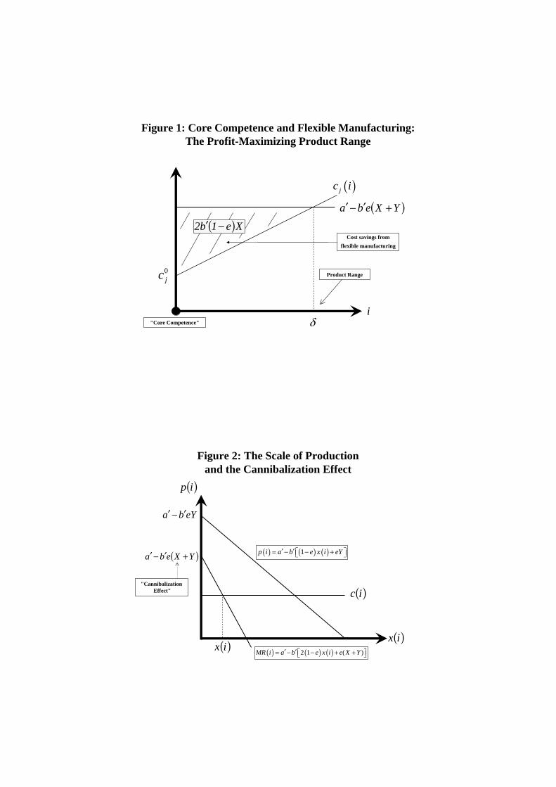
( )YXeba +′−′

δi

( )Xe1b2 −′

"Core Competence"

Product Range

Cost savings fromflexible manufacturing

( )jc i

Figure 1: Core Competence and Flexible Manufacturing:The Profit-Maximizing Product Range

0jc

Figure 2: The Scale of Productionand the Cannibalization Effect

eYba ′−′

( )YXeba +′−′

( )ix ( ) ( ) ( )2 1 ( )MR i a b e x i e X Y′ ′= − − + +⎡ ⎤⎣ ⎦

( )ic"Cannibalization

Effect"

( )ix

( )ip

( ) ( ) ( )1p i a b e x i eY′ ′= − − +⎡ ⎤⎣ ⎦

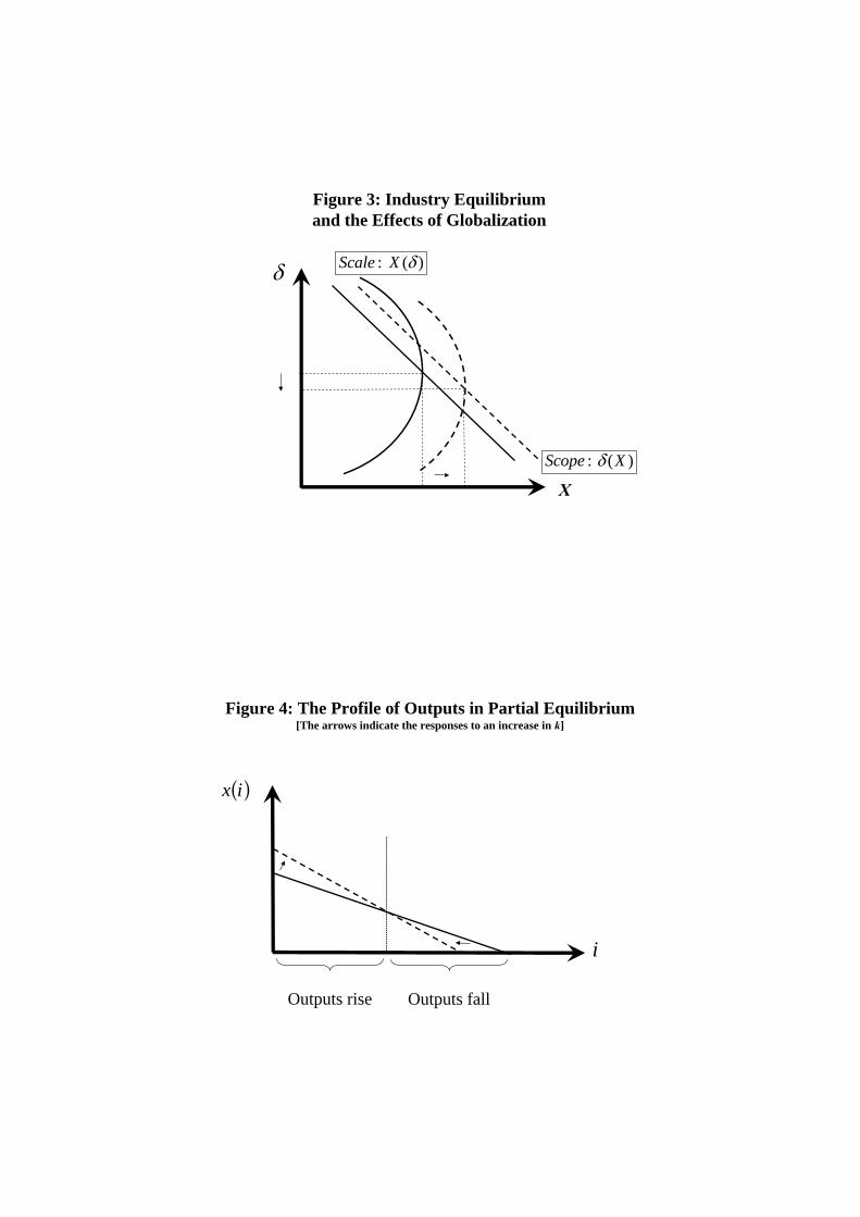
δ

Figure 3: Industry Equilibriumand the Effects of Globalization

X

: ( )Scope Xδ

: ( )Scale X δ

Figure 4: The Profile of Outputs in Partial Equilibrium[The arrows indicate the responses to an increase in k]

( )ix

i

Outputs rise Outputs fall

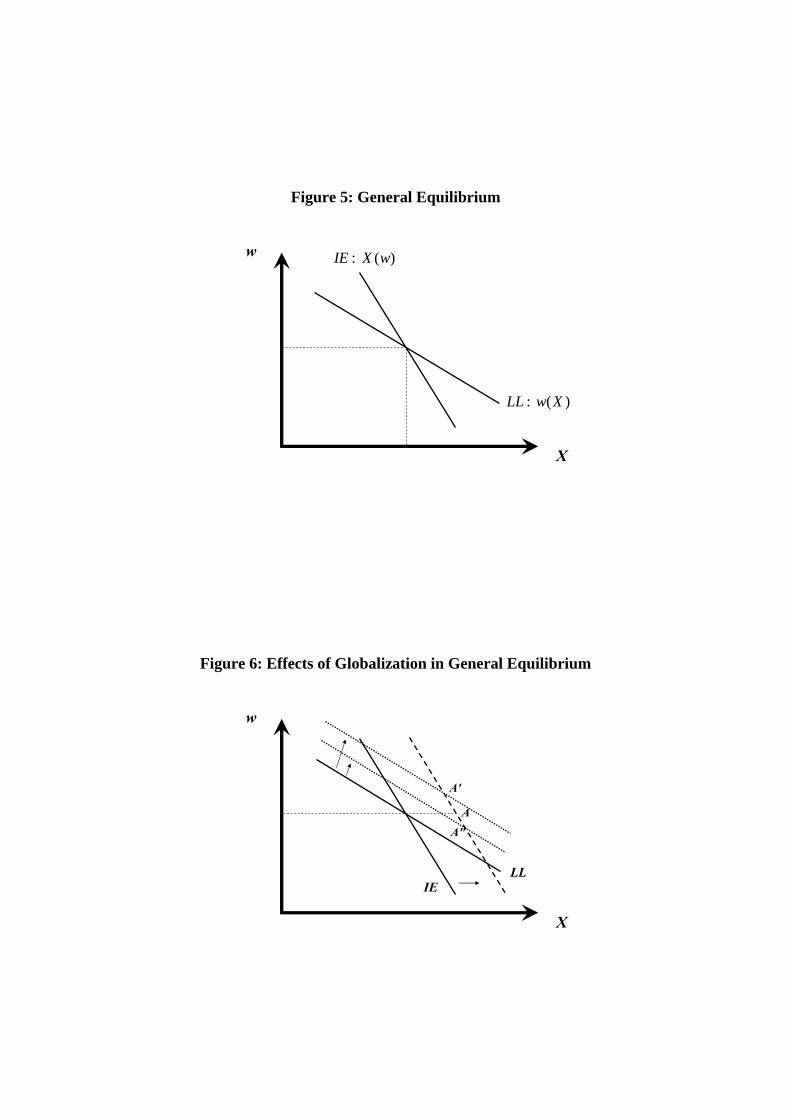
Figure 5: General Equilibrium

X

w : ( )IE X w

: ( )LL w X

Figure 6: Effects of Globalization in General Equilibrium

X

w

LLIE

A′

AA″