Multi-scale Assessment of Bone Mechanics and the Mineral

City University of New York (CUNY) City University of New York (CUNY)

CUNY Academic Works CUNY Academic Works

Dissertations and Theses City College of New York

2017

Multi-scale Assessment of Bone Mechanics and the Mineral Multi-scale Assessment of Bone Mechanics and the Mineral

Phase of Intramuscular Bone of Atlantic Herring Fish Phase of Intramuscular Bone of Atlantic Herring Fish

Svetlana Zeveleva CUNY City College

How does access to this work benefit you? Let us know!

More information about this work at: https://academicworks.cuny.edu/cc_etds_theses/708

Discover additional works at: https://academicworks.cuny.edu

This work is made publicly available by the City University of New York (CUNY). Contact: [email protected]

https://academicworks.cuny.edu/

https://academicworks.cuny.edu/cc_etds_theses

https://academicworks.cuny.edu/cc

http://ols.cuny.edu/academicworks/?ref=https://academicworks.cuny.edu/cc_etds_theses/708

https://academicworks.cuny.edu/cc_etds_theses/708

https://academicworks.cuny.edu/?

mailto:[email protected]

Multi-scale Assessment of Bone Mechanics and the Mineral Phase of Intramuscular Bone of Atlantic Herring Fish

THESIS

Submitted in partial fulfillment of

The requirement for the degree

Master of Science (Biomedical Engineering)

At

The City College

of the

City University of New York

By

Svetlana Zeveleva

December 2017

Approved:

_________________________________________ Professor Jean-Philippe Berteau, Thesis Advisor

Affiliated Faculty to the New York Center for Biomedical Engineering at City College

_________________________________________ Professor Bingmei Fu, Master’s Advisor

_________________________________________ Professor Mitchell Schaffler, Chairman Department of Biomedical Engineering

ii

Abstract Bone tissue is a complex composite structure made up of a soft organic phase consisting of

collagen I and non-collagenous proteins, and a hard inorganic phase consisting of mineral

nanoplatelets. Given it’s compositional properties, bone is a unique stiff, tough, and strong

biomaterial, making it exceptionally difficult to synthesize ex vivo. While the complete

hierarchical structure may change with age and population, the basic building block components

of mineralized collagen fibrils, are preserved. This study uses a model of intramuscular bone of

the Atlantic herring fish, which present a simple structure, and no process of remodeling.

A multi-scale approach was developed to measure mechanical properties, mineral composition,

mineral maturity or stoichiometric perfection, and distribution based on crystal thickness of 610

bone samples. Tensile modulus increased with tissue maturity marking an increased stiffness in

mature populations. Calcium to phosphate ratio showed a correlated increase with stiffness and

maturation along with carbonate content in the mineral component. Crystallinity ratio decreased

with maturation confirming the presence of carbon substitutions with maturation. Finally,

nanoscopic mineral crystal distribution resulted in thickening of crystals with maturation. This

assessment of the mineral component, along with micro-mechanical tensile tests showed that the

collagen-mineral interphase plays a key role in resisting load. These results contribute to a global

understanding between biological components at the Nano scale and mechanical behavior at the

macro-scale.

iii

Acknowledgments

I would like to thank Dr. Jean-Philippe Berteau for guiding me throughout my research and for his endless support in writing this thesis. His faith in my project and mentorship throughout my Master’s degree has helped me become the ambitious scientist that I am today. I would also like to express my gratitude to Dr. Bingmei Fu for her advisement and eagerness to help me succeed. I am grateful for all of our collaborators: Dr. Luis Cardoso, Dr. Sebastien Poget, Dr. Alan Lyons, and Dr. Shi Jin. In particular, I’d like to thank Dr. Luis Cardoso for being patient and acknowledging an experimental urgency and making it a priority to help us resolve it. Additionally I’d like to thank Annalisa De Paolis who designated hours on end to ensure that our µCT scans turned out perfect. I would also like to thank Xizhe Zhao for training me on infrared spectroscopy and Illya Nayshevsky for his guidance with thermal analysis methods. I would like to thank my lab mates. I am thankful to Abil Zia for firstly welcoming me into the lab and secondly for training me on dissection and bone processing protocols. I’m thankful to Imke Fiedler for always being responsive to my technical issues, Melody Labrune and Brahim Mehadji for their help with data analysis, and Clemence Fayolle for being ever so supportive and patient when science was turning its back on us. Lastly I’d like to dedicate this thesis to my family and friends, particularly Marina Ruvinova and Esther Goldenberg, who handled all of my complaints and frustrations throughout these two years. Without their affirmation that I can indeed overcome all sorts of challenges, I wouldn’t have made it this far and I am eternally grateful for their faith in me.

iv

Table of Contents 1. Introduction ............................................................................................................................................. 1

1.1 Mechanical Properties ......................................................................................................................... 1

1.2 Bone Ultrastructure ............................................................................................................................. 2

1.3 Relationship between biological components and mechanical behavior ............................................ 4

1.4 Bone maturation: mineralization and collagen maturation ................................................................. 5

1.5 TC-cAp Interactions ............................................................................................................................ 6

1.6 Animal model: Mammalians and The Atlantic herring (Clupaus Harengus) ..................................... 8

1.7 Aim of this study ................................................................................................................................. 9

2. Materials and methods .......................................................................................................................... 10

2.1 Outline of experiments ...................................................................................................................... 10

2.1.1 Sample Extraction ...................................................................................................................... 10

2.1.2 Multi-scale Assessment of Mineral ........................................................................................... 11

2.2 Macro-scale: Geometrical Properties ................................................................................................ 12

2.2.1 Basic Principles ......................................................................................................................... 12

2.2.2 Sample Preparation ................................................................................................................... 13

2.2.3 Acquisition Protocol .................................................................................................................. 13

2.2.4 Data Processing ......................................................................................................................... 13

2.3 Mechanical Properties ....................................................................................................................... 14



2.3.3 Loading Protocol ....................................................................................................................... 14

2.3.4 Data Processing ......................................................................................................................... 15

2.4 Macro-scale: Compositional Properties ............................................................................................ 16




2.4.4 Data Processing ......................................................................................................................... 18

2.5 Molecular-scale: Assessment of Mineral Component ....................................................................... 19




v

2.5.4 Data Processing ......................................................................................................................... 21

2.6 Nanoscale: Distribution of Mineral .................................................................................................. 22




2.7 Statistical Analysis ........................................................................................................................... 25

3. Results .................................................................................................................................................... 26

3.1 Macro-scale: Geometrical Properties ................................................................................................ 26





4. Discussion ............................................................................................................................................... 34





5. Conclusion .............................................................................................................................................. 42

6. References .............................................................................................................................................. 43

7. Appendix ................................................................................................................................................ 49

1

1 Introduction Bone is a hierarchized and intricate composite material made of a hard inorganic phase of

mineral apatite (Carbonate Apatite, cAp) and a soft organic phase (collagen type 1,

tropocollagen, TC) [1]–[3]. There are two types of bone tissue, cortical bone is the compact

intramembranous bone whereas trabecular is the spongy, endochondral bone. Although their

origin and porosity vary, at the tissue scale, their basic components of tropocollagen and mineral

are similar. Bone tissue is considered an engineering marvel due to the structure’s ability to

withstand intense loads over several hierarchical structures[2]. Regardless of bone location, bone

tissue mechanics is a unique combination of high stiffness, toughness and strength that remain

difficult to replicate. It has been established that the intermolecular forces at the collagen-mineral

interface (TC-cAp) are keys to understanding the mechanical behavior of bone tissue[5].

Biological components such as non-collagenous proteins code for calcium binding genes that

control the mineralization process within fibrils. Hence bonding within the interface is monitored

by genetic control as well.

The introduction of this master thesis is divided into five parts. The first sub-chapter presents the

mechanical role of bone tissue. The second sub-chapter presents the compositional breakdown

from whole bone to bone tissue. The third sub-chapter presents the relationship between

biological components and mechanical behavior of bone tissue. The fourth sub-chapter presents

the maturation of each bone component. The fifth sub-chapter focuses on a nano-scale mineral

assessment and its’ role in resisting deformation. The last sub-chapter proposes the aim of this

study.

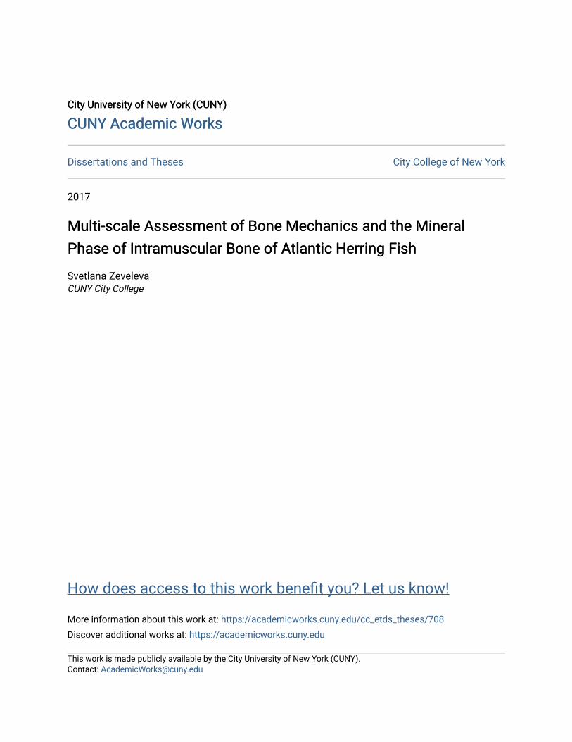
1.1 Mechanical Properties Mechanical properties can be distinguished into two parts: stiffness and toughness. Regarding

stiffness, the young’s modulus (E) is an appropriate measure corresponding to initial elastic

deformation (Figure 1-1). E values range from 5-21 GPa in whole cortical bone[6]. Regarding

toughness, total work (Wtot), is considered an appropriate measure, also corresponding with the

energy dissipated during fracture. Wtot values range from 50-70 MPa in whole cortical bone[6].

2

The yield point marks the maximum stress and strain before plastic deformation is initiated. At

that point, the bone becomes irreversibly elongated or deformed.

E

Figure 1-1: Typical stress-strain curve for macro-scale tensile test on bone tissue adapted from [7]. Wtot is a measure of toughness and E is a measure of stiffness. 1.2 Bone ultrastructure Compositional elements consist of mineral, collagen I, non-collagenous proteins, and water [1].

In the cortical bone, several hierarchical structures have been identified as shown in Figure 1-

2[8].

3

Figure 1-1: Compositional structure of bone at the macro, micro, and nano-scale. Image adapted from Rho et al 1998 [11][6]. At the micro-scale (tissue level), lamellar bone is made of tropocollagen fibers assembled into

lamellar packets and furthermore into cylindrical structures known as osteons. At the nano-scale,

these fibers are made up of tropocollagen fibrils (TC) and carbonate hydroxyapatite mineral

crystals (cAp), otherwise known as mineralized collagen fibrils (MCF) [7], [8] . This

nanostructure is preserved amongst all vertebrates. These fibrils consist of tropocollagen

molecules arranged in a quarter- staggered alignment[9]–[11] .Collagen fibrils periodically

present gap regions of ~40nm length and overlap regions of ~27 nm length [15][16][17]. Intra and

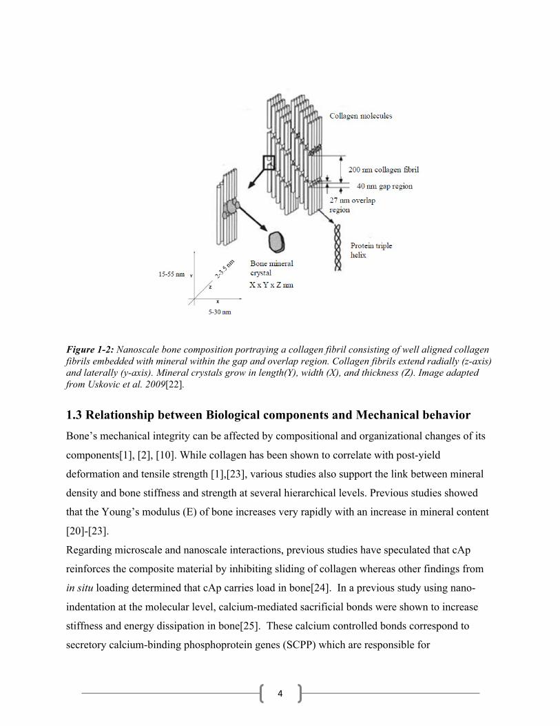
extra-fibrillar bone mineral crystals have dimensions of up to 15-55 nm in length, up to 5-30 nm

in width, and 2-3.5 nm in thickness (Figure 1-2) [1][10][15][18][19].

Therefore the mineralized collagen fibrils are often referred to as the main building blocks of

bone. TC-cAp interaction within the MCF is a result of electrostatic interactions and hydrogen

bonding [20]. Hydrogen bonding occurs solely between the chains of the collagen molecules and

even more often where mineral is present (gap region)[20]. Another important mechanism of

load transfer between collagen and mineral is due to salt bridges (electrostatic interactions

between charged moieties)[20]. Although in the non-mineralized fibril this type of non-covalent

interaction is minor, it becomes rather important in the mineralized samples. Salt bridges are

formed within the mineral crystals; however, the majority are formed between mineral crystals

and collagen, providing an effective load transfer mechanism between the mineral and organic

phase that also enhances material toughness[21].

4

Figure 1-2: Nanoscale bone composition portraying a collagen fibril consisting of well aligned collagen fibrils embedded with mineral within the gap and overlap region. Collagen fibrils extend radially (z-axis) and laterally (y-axis). Mineral crystals grow in length(Y), width (X), and thickness (Z). Image adapted from Uskovic et al. 2009[22].

1.3 Relationship between Biological components and Mechanical behavior Bone’s mechanical integrity can be affected by compositional and organizational changes of its

components[1], [2], [10]. While collagen has been shown to correlate with post-yield

deformation and tensile strength [1],[23], various studies also support the link between mineral

density and bone stiffness and strength at several hierarchical levels. Previous studies showed

that the Young’s modulus (E) of bone increases very rapidly with an increase in mineral content

[20]-[23].

Regarding microscale and nanoscale interactions, previous studies have speculated that cAp

reinforces the composite material by inhibiting sliding of collagen whereas other findings from

in situ loading determined that cAp carries load in bone[24]. In a previous study using nano-

indentation at the molecular level, calcium-mediated sacrificial bonds were shown to increase

stiffness and energy dissipation in bone[25]. These calcium controlled bonds correspond to

secretory calcium-binding phosphoprotein genes (SCPP) which are responsible for

5

mineralization of the fibrils. SCPP genes are found in non-collagenous proteins (NCPs) within

bone[26]. Additionally, NCPs in antler MCF were shown to strengthen fairly week bonds,

producing a tougher material[27] [28]. While a long term paradigm has associated the collagen

phase to toughness and the mineral phase to stiffness, it has also been suggested that

intermolecular forces at the collagen-mineral interface (TC-cAp) are key to understanding the

mechanical behavior of bone tissue. However, recent results have shown variation due to

species, gender, and age of the bone studied, making it difficult to establish the relationship

between intermolecular forces at the TC-cAp interface and bone macro-scopic mechanical

behavior.

1.4 Bone maturation: mineralization and collagen maturation During tissue maturation, collagen fibrils and mineral crystals mature concurrently. Collagen

maturity is determined by the ratio of mature to immature cross-links, while mineral maturity is

described by the crystal size, shape, and deposition within the laden collagen fibrils (intra or

extrafibrillar). The first step of maturation is the deposition of the collagen matrix. Lysyl

oxidases act on lysine and hydroxylysine residues in the telopeptide regions of fibrillar collagen

resulting in the formation of the normal non-enzymatic and enzymatic collagen cross-links [29].

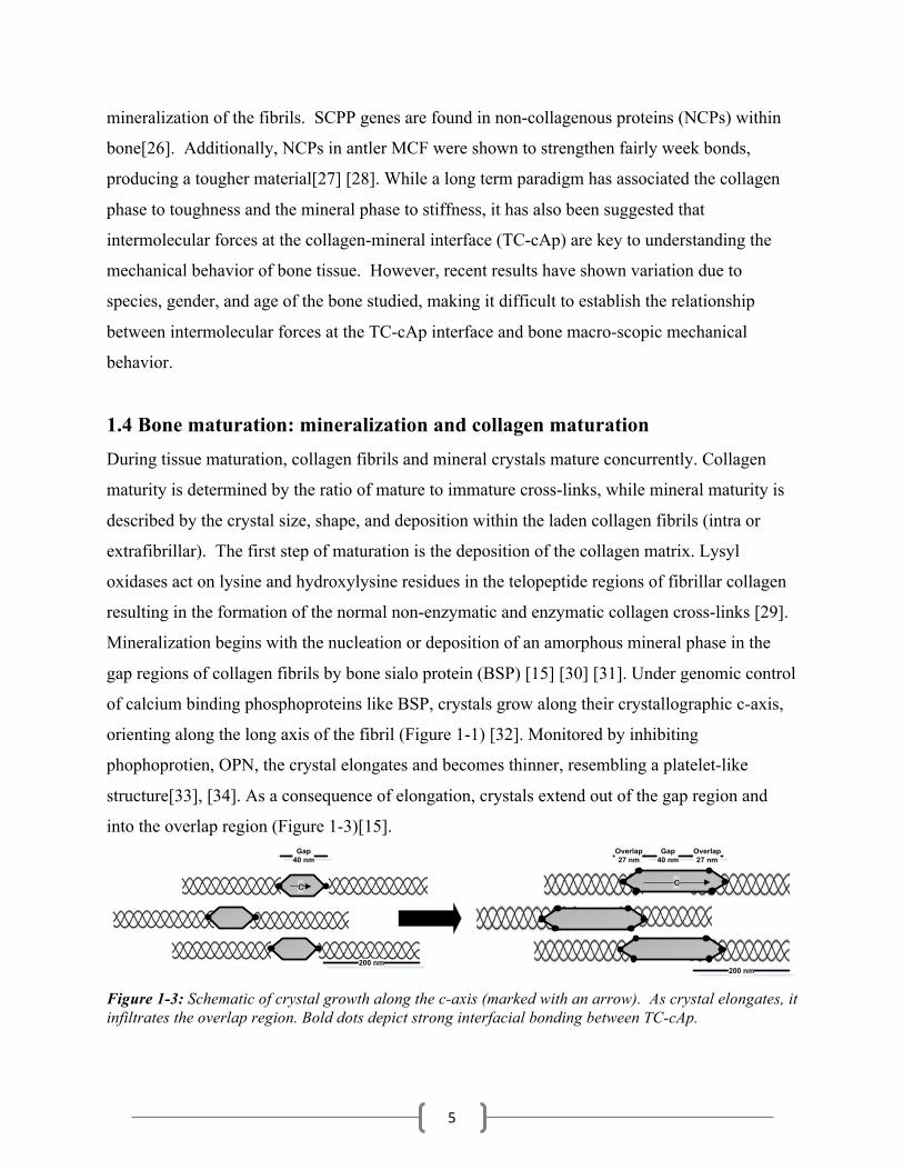
Mineralization begins with the nucleation or deposition of an amorphous mineral phase in the

gap regions of collagen fibrils by bone sialo protein (BSP) [15] [30] [31]. Under genomic control

of calcium binding phosphoproteins like BSP, crystals grow along their crystallographic c-axis,

orienting along the long axis of the fibril (Figure 1-1) [32]. Monitored by inhibiting

phophoprotien, OPN, the crystal elongates and becomes thinner, resembling a platelet-like

structure[33], [34]. As a consequence of elongation, crystals extend out of the gap region and

into the overlap region (Figure 1-3)[15]. Gap

40 nmOverlap27 nm

Gap40 nm

Overlap27 nm

200 nm200 nm

c c

Figure 1-3: Schematic of crystal growth along the c-axis (marked with an arrow). As crystal elongates, it infiltrates the overlap region. Bold dots depict strong interfacial bonding between TC-cAp.

6

Growing cAp nano-platelets distort the collagen array (not shown) and result in mechanical

interlocking[5]. This process is also accompanied by changes in chemical composition of the

mineral. During maturation, carbonate substitution in the apatite crystal occur in the hydroxyl

and/or the phosphate sites. During the second step of tissue mineralization, intra-fibrillar crystals

emerge into the extra-fibrillar space, leading to a further increase in mineral mass[32].

1.5 TC-cAp Interactions At the nano-scale, it has been established that mineral crystals increase the stiffness but decrease

the fracture strain of collagen fibrils[11],[8]. In support of this, Landis et al. presented that the

young’s modulus increases with the amount of mineral deposited in the collagen structure, up to

a factor of 400[10]. To better understand why these mechanical parameters act in such a way at

the nano-scale, Depalle et al. presented that a MCF can undergo a four step deformation

mechanisms as depicted in Figure 1-3. During phase I, most of the elastic deformation arises in

the overlap region because mineral restrains deformation in the gap region. Due to some sliding

between mineral and collagen, the load is transferred to the collagen molecules. In phase II

because TC-cAp energy is not sufficient enough to sustain load, slippage between TC-cAp and

cAp-cAp occurs in the gap region until the mineral dissociates. During phase III collagen fibrils

experience backbone stretching until ultimate failure occurs in phase IV.

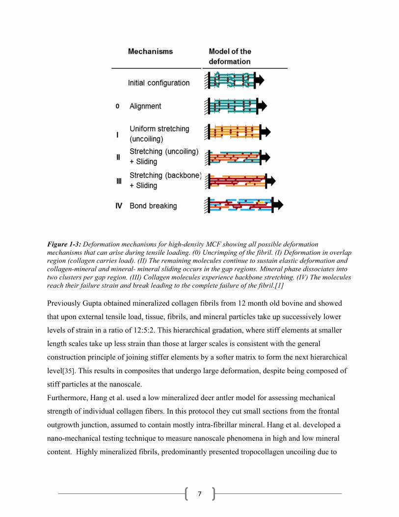
7

Figure 1-3: Deformation mechanisms for high-density MCF showing all possible deformation mechanisms that can arise during tensile loading. (0) Uncrimping of the fibril. (I) Deformation in overlap region (collagen carries load). (II) The remaining molecules continue to sustain elastic deformation and collagen-mineral and mineral- mineral sliding occurs in the gap regions. Mineral phase dissociates into two clusters per gap region. (III) Collagen molecules experience backbone stretching. (IV) The molecules reach their failure strain and break leading to the complete failure of the fibril.[1] Previously Gupta obtained mineralized collagen fibrils from 12 month old bovine and showed

that upon external tensile load, tissue, fibrils, and mineral particles take up successively lower

levels of strain in a ratio of 12:5:2. This hierarchical gradation, where stiff elements at smaller

length scales take up less strain than those at larger scales is consistent with the general

construction principle of joining stiffer elements by a softer matrix to form the next hierarchical

level[35]. This results in composites that undergo large deformation, despite being composed of

stiff particles at the nanoscale.

Furthermore, Hang et al. used a low mineralized deer antler model for assessing mechanical

strength of individual collagen fibers. In this protocol they cut small sections from the frontal

outgrowth junction, assumed to contain mostly intra-fibrillar mineral. Hang et al. developed a

nano-mechanical testing technique to measure nanoscale phenomena in high and low mineral

content. Highly mineralized fibrils, predominantly presented tropocollagen uncoiling due to

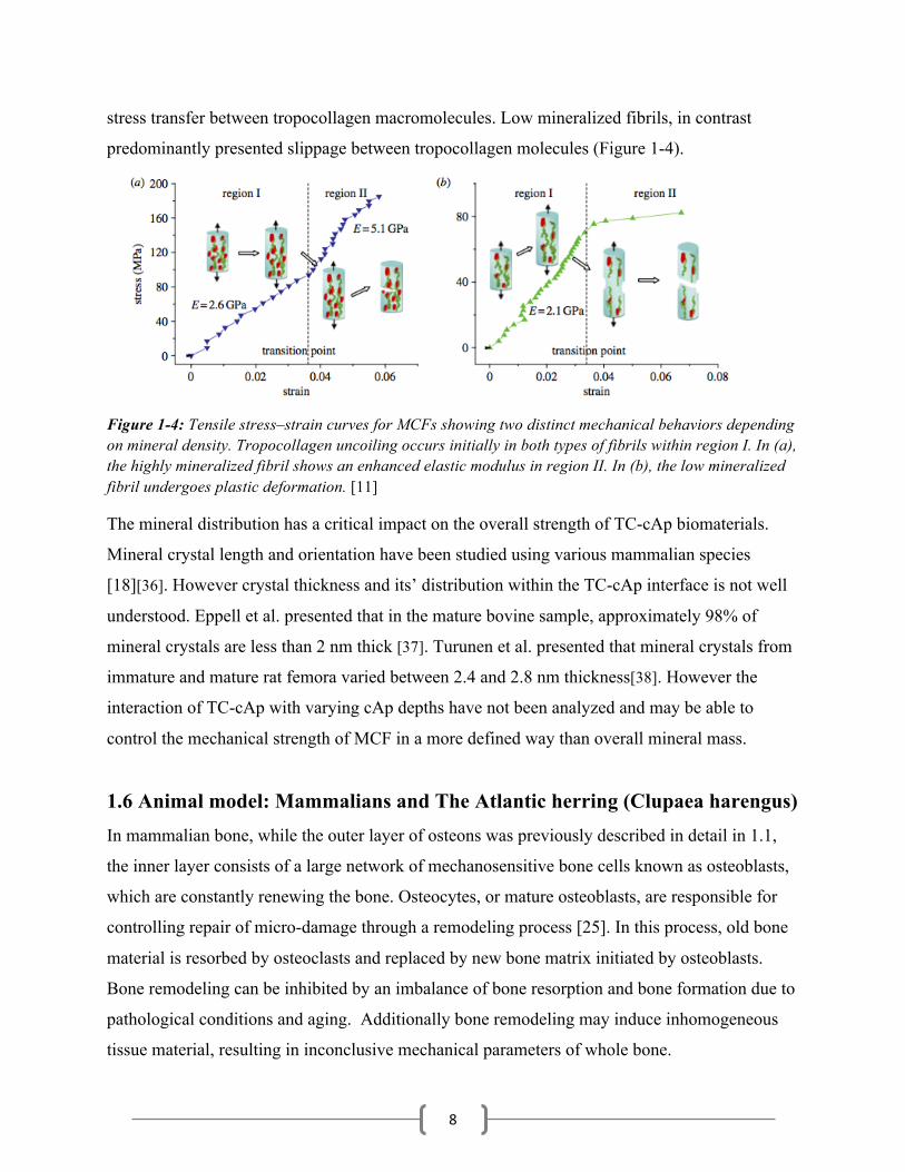
8

stress transfer between tropocollagen macromolecules. Low mineralized fibrils, in contrast

predominantly presented slippage between tropocollagen molecules (Figure 1-4).

Figure 1-4: Tensile stress–strain curves for MCFs showing two distinct mechanical behaviors depending on mineral density. Tropocollagen uncoiling occurs initially in both types of fibrils within region I. In (a), the highly mineralized fibril shows an enhanced elastic modulus in region II. In (b), the low mineralized fibril undergoes plastic deformation. [11]

The mineral distribution has a critical impact on the overall strength of TC-cAp biomaterials.

Mineral crystal length and orientation have been studied using various mammalian species

[18][36]. However crystal thickness and its’ distribution within the TC-cAp interface is not well

understood. Eppell et al. presented that in the mature bovine sample, approximately 98% of

mineral crystals are less than 2 nm thick [37]. Turunen et al. presented that mineral crystals from

immature and mature rat femora varied between 2.4 and 2.8 nm thickness[38]. However the

interaction of TC-cAp with varying cAp depths have not been analyzed and may be able to

control the mechanical strength of MCF in a more defined way than overall mineral mass.

1.6 Animal model: Mammalians and The Atlantic herring (Clupaea harengus) In mammalian bone, while the outer layer of osteons was previously described in detail in 1.1,

the inner layer consists of a large network of mechanosensitive bone cells known as osteoblasts,

which are constantly renewing the bone. Osteocytes, or mature osteoblasts, are responsible for

controlling repair of micro-damage through a remodeling process [25]. In this process, old bone

material is resorbed by osteoclasts and replaced by new bone matrix initiated by osteoblasts.

Bone remodeling can be inhibited by an imbalance of bone resorption and bone formation due to

pathological conditions and aging. Additionally bone remodeling may induce inhomogeneous

tissue material, resulting in inconclusive mechanical parameters of whole bone.

9

To overcome this limitation, this study will adapt a piscine (fish) model. Fugu, Zebrafish, and

Nile tilapia have illuminated the presence of SCPP genes which control the process of fibril

mineralization[34], [39]–[41]. SCPP genes are expressed by non-collagenous phosphoproteins

that control crystal infiltration and growth. In most teleost models, SCPP genes have been

referenced to their aliases in human: IBSP (BSP) and SPP1 (OPN) which assist or resist

infiltration of cAp, respectively [39], [40]. Previous publications have proposed that the intra-

muscular bones of the Atlantic herring (IMAH) fish avoid complex structures such as osteons

and lamellae [5]. Moreover, they do not present osteocytes, vascularization, or porosity[42].

Although the whole bone structure may vary with gender, mammalian species, etc., the main

building blocks of intra-fibrillar MCF are conserved. This unique structure of IMAH can be

considered simplified human bone. The absence of remodeling suggests that IMAH host solely

intra-fibrillar mineral exemplifying the early stage of maturation[41]-[42].

Hence, it can be also be assumed that the fish age corresponds to the bone tissue age [43]. Given

its’ unique and simple characteristics, IMAH bones suggest a unique model for characterization.

1.7 Aim of this study

The aim of this study is to investigate the mineral composition of bone and its relation to the

mechanical properties of intra-fibrillar MCFs. This study proposes that local crystal geometry

and composition is a key factor for TC-cAp bonding and a determinant of mechanical

performance in bone. To test this hypothesis a model of IMAH of varying maturity was chosen

to explore structural and mechanical changes at different stages of early tissue maturation. The

results presented here open new possibilities in designing biomaterials that capture the intrinsic

mechanical features of mineralized collagen fibrils.

10

2 Material and methods A multiscale approach was designed to investigate the mineral phase and bone mechanics of

IMAH. Chapter 2.1 outlines the experimental protocols and overall study layout. Chapters 2.2-

2.6 described these sections include an overview of theoretical principles, sample preparation,

acquisition protocols, and data processing techniques of each experimental technique. Chapter 2-

7 describes the statistical analysis used for each data analysis.

2.1 Outline of experiments This first subchapter will introduce sample retrieval and subsequently describes the step-wise

approach to investigating present bone samples. First the geometrical properties were calculated,

then mechanical properties are determined, followed by the assessment of compositional

properties at the macro and molecular scale, and lastly nanoscopic mineral distribution was

studied.

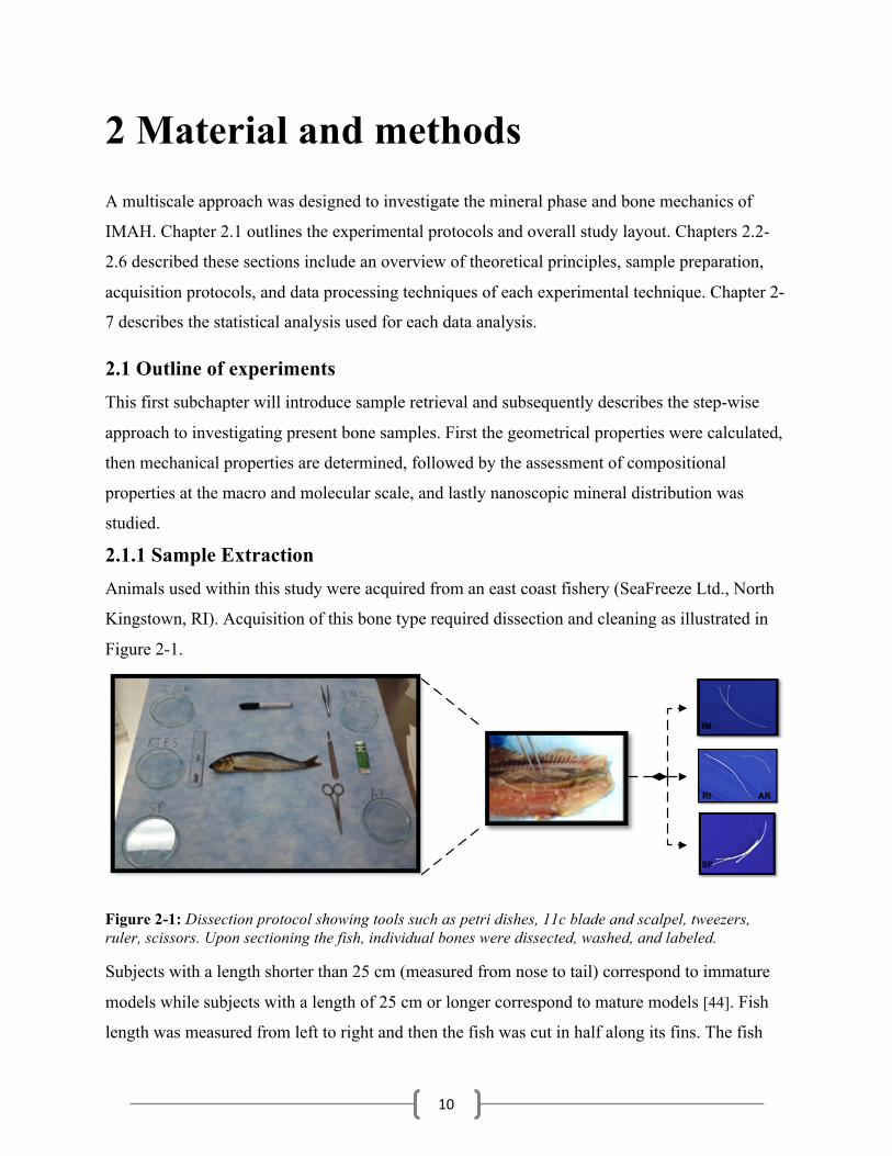
2.1.1 Sample Extraction Animals used within this study were acquired from an east coast fishery (SeaFreeze Ltd., North

Kingstown, RI). Acquisition of this bone type required dissection and cleaning as illustrated in

Figure 2-1.

RI AR

IM

SP

Figure 2-1: Dissection protocol showing tools such as petri dishes, 11c blade and scalpel, tweezers, ruler, scissors. Upon sectioning the fish, individual bones were dissected, washed, and labeled.

Subjects with a length shorter than 25 cm (measured from nose to tail) correspond to immature

models while subjects with a length of 25 cm or longer correspond to mature models [44]. Fish

length was measured from left to right and then the fish was cut in half along its fins. The fish

11

bones were sectioned into right and left skeletal bones. Dissected bones were then categorized

into five groups: IM_R (intramuscular right), IM_L (intramuscular left), RI (ribs), SP_NH

(spinal neural humorous), and AR (all of the rest). Bones were washed in phosphate buffered

solution, PBS (MP Biomedical LLC, Solon, OH) on a stirrer (Fisher Scientific Isotemp Stirrer).

The bones were then dried, weighed, and counted. Each bone category was individually labeled

and stored for further processing in gauze soaked in PBS and protein inhibitor, PI (bioWorld,

Dublin, OH).

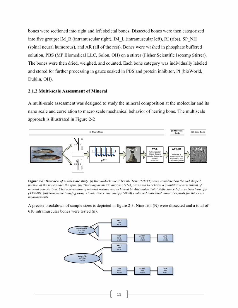
2.1.2 Multi-scale Assessment of Mineral

A multi-scale assessment was designed to study the mineral composition at the molecular and its

nano scale and correlation to macro scale mechanical behavior of herring bone. The multiscale

approach is illustrated in Figure 2-2

TGA-% Composition (Water, Organic

Material, Carbonate, Mineral)

-Ca/P ratio

ATR-IR

-Absence of organic materials -Crystallinity ratio-Crystallinity Index

(i) Macro Scale (ii) Molecular Scale (iii) Nano Scale

MMTT AFM

5µm

8mm

µCT

A

J

8mm

Figure 2-2: Overview of multi-scale study. (i)Micro-Mechanical Tensile Tests (MMTT) were completed on the rod shaped portion of the bone under the spur. (ii) Thermogravimetric analysis (TGA) was used to achieve a quantitative assessment of mineral composition. Characterization of mineral residue was achieved by Attenuated Total Reflectance Infrared Spectroscopy (ATR-IR). (iii) Nanoscale imaging using Atomic Force microscopy (AFM) evaluated individual mineral crystals for thickness measurements.

A precise breakdown of sample sizes is depicted in figure 2-3. Nine fish (N) were dissected and a total of 610 intramuscular bones were tested (n).

TGAN= 3

n=233

MMTTN=1n=24

TGAN= 3

n=305

MMTTN=1n=24

ATR-IRN=3

n=240

AFMN=2

n=145

AFMN=1n=81

ATR-IRN=3

n=233

ATR-IRN=3

n=233

Immature (IM)N=4 Fish

n=341

Mature (M)N=5 Fish

n=269

12

Figure 2-3: Overview of sample size breakdown based on techniques used for multi-scale assessment.

2.2 Macro-scale: Geometrical Properties

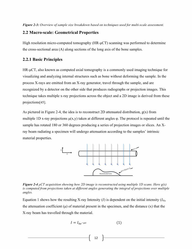
High resolution micro-computed tomography (HR-µCT) scanning was performed to determine

the cross-sectional area (A) along sections of the long axis of the bone samples.

2.2.1 Basic Principles

HR-µCT, also known as computed axial tomography is a commonly used imaging technique for

visualizing and analyzing internal structures such as bone without deforming the sample. In the

process X-rays are emitted from an X-ray generator, travel through the sample, and are

recognized by a detector on the other side that produces radiographs or projection images. This

technique takes multiple x-ray projections across the object and a 2D image is derived from these

projections[45].

As pictured in Figure 2-4, the idea is to reconstruct 2D attenuated distribution, g(x) from

multiple 1D x-ray projections µ(x,y) taken at different angles φ. The protocol is repeated until the

sample has rotated 180 or 360 degrees producing a series of projection images or slices. An X-

ray beam radiating a specimen will undergo attenuation according to the samples’ intrinsic

material properties.

x

y

µ(x,y)

g(x)=ʃdyµ(

x,y)

Reconstructed bone

Figure 2-4 µCT acquisition showing how 2D image is reconstructed using multiple 1D scans. Here g(x) is computed from projections taken at different angles generating the integral of projections over multiple angles.

Equation 1 shows how the resulting X-ray Intensity (𝐼) is dependent on the initial intensity (𝐼0),

the attenuation coefficient (µ) of material present in the specimen, and the distance (x) that the

X-ray beam has travelled through the material.

𝐼 = 𝐼!!!!" (1)

13

Using fan- or cone-beam X-ray radiation to scan a rotating sample from different angles then

allows for 2D images reconstruction. Voxel sizes of <10 µm are commonly acquired, whereby a

smaller spatial resolution would require a higher scan time[46].

2.2.2 Sample Preparation Prior to scanning, (3mm) sections under the spur were marked for visualization. Individual

samples were wrapped in gauze and placed in individual Eppendorf tubes to be used for high

resolution micro computed tomography (HR- µCT) imaging.

2.2.3 Acquisition Protocol Prepared samples were positioned in a custom-made acrylic sample holder featuring twelve pits

with a diameter of 1.2 mm and a depth of approximately 4mm. Scans were acquired using an

HR- µCT (SkyScan 1172, Bruker, Kontich, BE) at a resolution of 5.05 µm, X-ray voltage of 100

kV and current of 100 µA. Each scan included twelve samples and was performed within 2

hours. Two scans were performed in this study in Dr.Luis Cardoso’s lab.

2.2.4 Data Processing Reconstruction of native gray scale images was performed with an in-house software, CTAn

(V.1.10.1., Skyscan, Bruker, BE). Using the CTAn software, stacks of cropped slices of

individual bones were attained. The mean cross-sectional area was determined using a custom

MatLab script where pixel area was converted to real area using the resolution conversion of

5.01 µm per pixel (A.3.1.1). Equation 3 serves as the conversion where AP is total pixel area, and

ACS is the cross-sectional area of the bone slice in mm2.

𝐴!! = 𝐴!5.01! ∗ 10!! (3)

(ii)

(iii)

(i) (iv)

14

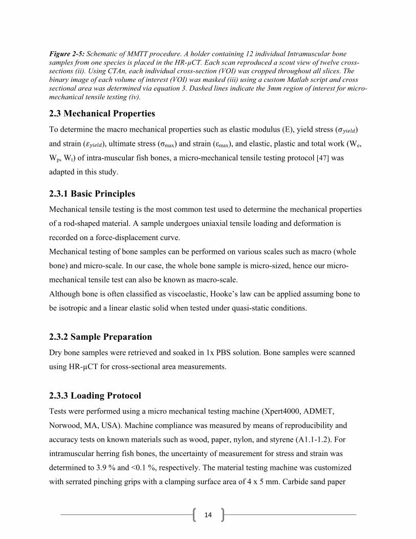
Figure 2-5: Schematic of MMTT procedure. A holder containing 12 individual Intramuscular bone samples from one species is placed in the HR-µCT. Each scan reproduced a scout view of twelve cross-sections (ii). Using CTAn, each individual cross-section (VOI) was cropped throughout all slices. The binary image of each volume of interest (VOI) was masked (iii) using a custom Matlab script and cross sectional area was determined via equation 3. Dashed lines indicate the 3mm region of interest for micro-mechanical tensile testing (iv).

2.3 Mechanical Properties To determine the macro mechanical properties such as elastic modulus (E), yield stress (𝜎𝑦𝑖𝑒𝑙𝑑)

and strain (𝜀𝑦𝑖𝑒𝑙𝑑), ultimate stress (σmax) and strain (εmax), and elastic, plastic and total work (We,

Wp, Wt) of intra-muscular fish bones, a micro-mechanical tensile testing protocol [47] was

adapted in this study.

2.3.1 Basic Principles Mechanical tensile testing is the most common test used to determine the mechanical properties

of a rod-shaped material. A sample undergoes uniaxial tensile loading and deformation is

recorded on a force-displacement curve.

Mechanical testing of bone samples can be performed on various scales such as macro (whole

bone) and micro-scale. In our case, the whole bone sample is micro-sized, hence our micro-

mechanical tensile test can also be known as macro-scale.

Although bone is often classified as viscoelastic, Hooke’s law can be applied assuming bone to

be isotropic and a linear elastic solid when tested under quasi-static conditions.

2.3.2 Sample Preparation Dry bone samples were retrieved and soaked in 1x PBS solution. Bone samples were scanned

using HR-µCT for cross-sectional area measurements.

2.3.3 Loading Protocol Tests were performed using a micro mechanical testing machine (Xpert4000, ADMET,

Norwood, MA, USA). Machine compliance was measured by means of reproducibility and

accuracy tests on known materials such as wood, paper, nylon, and styrene (A1.1-1.2). For

intramuscular herring fish bones, the uncertainty of measurement for stress and strain was

determined to 3.9 % and <0.1 %, respectively. The material testing machine was customized

with serrated pinching grips with a clamping surface area of 4 x 5 mm. Carbide sand paper

15

(P500) was glued onto the clamping surface to prevent samples from slipping when gripped. The

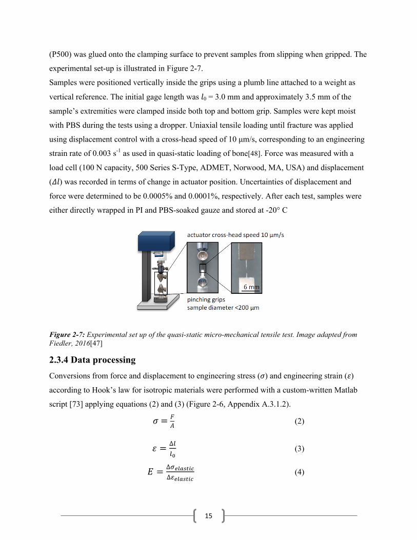
experimental set-up is illustrated in Figure 2-7.

Samples were positioned vertically inside the grips using a plumb line attached to a weight as

vertical reference. The initial gage length was 𝑙0 = 3.0 mm and approximately 3.5 mm of the

sample’s extremities were clamped inside both top and bottom grip. Samples were kept moist

with PBS during the tests using a dropper. Uniaxial tensile loading until fracture was applied

using displacement control with a cross-head speed of 10 µm/s, corresponding to an engineering

strain rate of 0.003 s-1 as used in quasi-static loading of bone[48]. Force was measured with a

load cell (100 N capacity, 500 Series S-Type, ADMET, Norwood, MA, USA) and displacement

(𝛥𝑙) was recorded in terms of change in actuator position. Uncertainties of displacement and

force were determined to be 0.0005% and 0.0001%, respectively. After each test, samples were

either directly wrapped in PI and PBS-soaked gauze and stored at -20° C

Figure 2-7: Experimental set up of the quasi-static micro-mechanical tensile test. Image adapted from Fiedler, 2016[47]

2.3.4 Data processing Conversions from force and displacement to engineering stress (𝜎) and engineering strain (𝜀)

according to Hook’s law for isotropic materials were performed with a custom-written Matlab

script [73] applying equations (2) and (3) (Figure 2-6, Appendix A.3.1.2).

𝜎 = 𝐹𝐴 (2)

𝜀 = ∆!!!

(3)

𝐸 = ∆!!"#$%&'∆!!"#$%&'

(4)

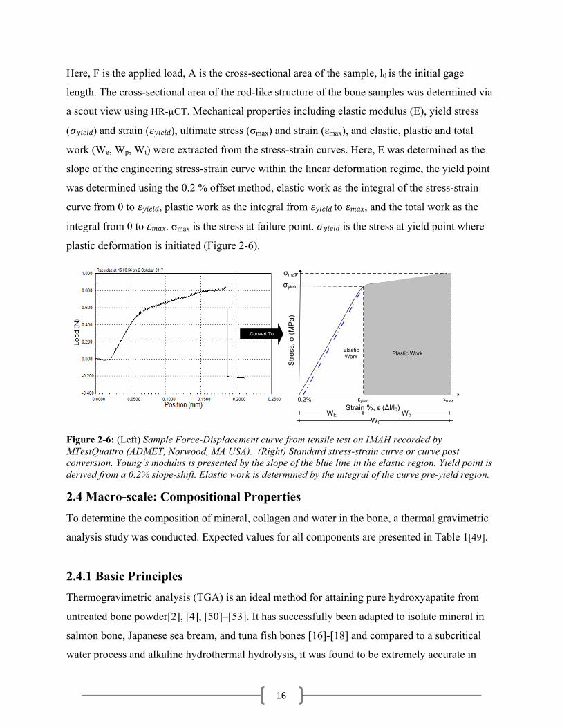
16

Here, F is the applied load, A is the cross-sectional area of the sample, l0 is the initial gage

length. The cross-sectional area of the rod-like structure of the bone samples was determined via

a scout view using HR-µCT. Mechanical properties including elastic modulus (E), yield stress

(𝜎𝑦𝑖𝑒𝑙𝑑) and strain (𝜀𝑦𝑖𝑒𝑙𝑑), ultimate stress (σmax) and strain (εmax), and elastic, plastic and total

work (We, Wp, Wt) were extracted from the stress-strain curves. Here, E was determined as the

slope of the engineering stress-strain curve within the linear deformation regime, the yield point

was determined using the 0.2 % offset method, elastic work as the integral of the stress-strain

curve from 0 to 𝜀𝑦𝑖𝑒𝑙𝑑, plastic work as the integral from 𝜀𝑦𝑖𝑒𝑙𝑑 to 𝜀𝑚𝑎𝑥, and the total work as the

integral from 0 to 𝜀𝑚𝑎𝑥. σmax is the stress at failure point. 𝜎𝑦𝑖𝑒𝑙𝑑 is the stress at yield point where

plastic deformation is initiated (Figure 2-6).

0.2% εyield εmax

Plastic WorkElastic Work

σyield

σmax

Stre

ss, σ

(MP

a)

Strain %, ε (Δl/l0) WpWEWt

Convert To

Figure 2-6: (Left) Sample Force-Displacement curve from tensile test on IMAH recorded by MTestQuattro (ADMET, Norwood, MA USA). (Right) Standard stress-strain curve or curve post conversion. Young’s modulus is presented by the slope of the blue line in the elastic region. Yield point is derived from a 0.2% slope-shift. Elastic work is determined by the integral of the curve pre-yield region.

2.4 Macro-scale: Compositional Properties To determine the composition of mineral, collagen and water in the bone, a thermal gravimetric

analysis study was conducted. Expected values for all components are presented in Table 1[49].

2.4.1 Basic Principles Thermogravimetric analysis (TGA) is an ideal method for attaining pure hydroxyapatite from

untreated bone powder[2], [4], [50]–[53]. It has successfully been adapted to isolate mineral in

salmon bone, Japanese sea bream, and tuna fish bones [16]-[18] and compared to a subcritical

water process and alkaline hydrothermal hydrolysis, it was found to be extremely accurate in

17

preserving crystal shape. Published electron diffraction images have verified that this thermal

process produces good crystallinity hydroxyapatite [16].

This method measures weight change (loss) and rate of weight change as a function of

temperature, time, and atmosphere. In TGA, a sample is heated in a stream of gas[51]. This

technique can be used to characterize materials that exhibit weight loss due to decomposition.

Decomposition is the breaking apart of hydrogen bonds and salt bridges as introduced in 1-2. In

this experiment, we use gravimetric analyses to isolate the hydroxyapatite mineral component of

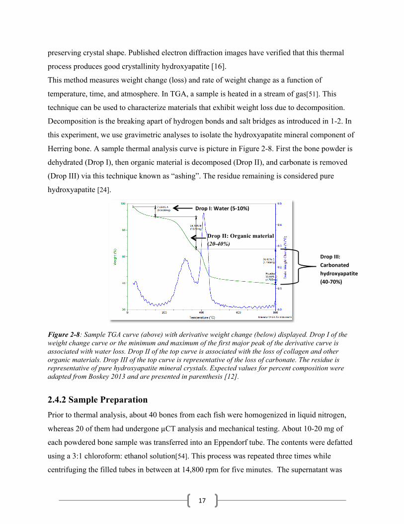
Herring bone. A sample thermal analysis curve is picture in Figure 2-8. First the bone powder is

dehydrated (Drop I), then organic material is decomposed (Drop II), and carbonate is removed

(Drop III) via this technique known as “ashing”. The residue remaining is considered pure

hydroxyapatite [24].

Figure 2-8: Sample TGA curve (above) with derivative weight change (below) displayed. Drop I of the weight change curve or the minimum and maximum of the first major peak of the derivative curve is associated with water loss. Drop II of the top curve is associated with the loss of collagen and other organic materials. Drop III of the top curve is representative of the loss of carbonate. The residue is representative of pure hydroxyapatite mineral crystals. Expected values for percent composition were adapted from Boskey 2013 and are presented in parenthesis [12].

2.4.2 Sample Preparation Prior to thermal analysis, about 40 bones from each fish were homogenized in liquid nitrogen,

whereas 20 of them had undergone µCT analysis and mechanical testing. About 10-20 mg of

each powdered bone sample was transferred into an Eppendorf tube. The contents were defatted

using a 3:1 chloroform: ethanol solution[54]. This process was repeated three times while

centrifuging the filled tubes in between at 14,800 rpm for five minutes. The supernatant was

DropI:Water(5-10%)

Drop II: Organic material (20-40%)

DropIII:Carbonatedhydroxyapatite(40-70%)

18

decanted each time. Upon completion of three iterations, bone powder was washed three times

with Millipore water while centrifuging in between for five minutes. Lids were removed and the

openings at the top of the tubes were wrapped with Kimtech (Kimberly-Clark Corporation,

Dallas, TX) wipes and tightened with rubber bands. The tubes of samples were placed upright in

a dry ice tub for 30 minutes to evaporate access water. Finally the samples were lyophilized for

48 hours before proceeding with the thermogravimetric analysis.

2.4.3 Acquisition Protocol Samples were transferred onto wax paper and pre-weighed. The platinum crucible from the TGA

was cleaned using heat treatment either by Bunsen burner or by simply ramping up the heat to

50°C. Samples were heated at a rate of 10°C/min in a chamber furnace with a stream of nitrogen

gas to 800°C and then cooled down to 30°C at 30°C/min before releasing the bone ash residue

similar to protocols for salmon and tuna bones published already [4], [52]. Each heat treatment

was carried out for 2 hours.

2.4.4 Data processing Results were analyzed using the TA Universal Analysis software. A derivative weight change

curve was plotted in a Weight loss vs. Temperature plot. The first peak of the derivative curve is

affiliated with dehydration or water loss, followed by organic material loss, and carbonate loss.

The remaining residue is suspected to be pure hydroxyapatite mineral. Percentage lost and

weight in mg is determined for each component. Native bone mineral is composed of carbonated

hydroxyapatite where molar coefficients are determined based on equations (6) and (7).

Assuming that the carbon dioxide arises from the breakdown of carbonate in the mineral, the

mass of carbonate lost is the change in mass from the last drop of the TGA analysis multiplied by

1.36 (the relative molecular masses of CO3 and CO2). Therefore the carbonate stoichiometric

coefficient is determined by equation (5) where C is the carbonate mass derived from the TGA

results and Mi is the initial mass of the bone powder inputted[51].

Bone mineral contains approximately 20% of the hydroxide groups, 20% of 2 is 0.4 leading to

equation (7). From equation (7), the molar coefficient of PO4, x, is then derived and the Ca/P

ratio is determined.

19

!∗!.!"∗!!!"#

= 𝑦 (5)

Ca!"[(PO!)!!!!! HPO! ! 𝐶𝑂! !][(OH)!!!!! 𝐶𝑂! ! (6)

2− 𝑥 − 𝑦 = 0.4 (7)

2.5 Molecular scale: Assessment of Mineral Component To determine the mineral crystal growth and perfection, a chemical analysis method most

commonly known as Fourier Transform Infrared Spectroscopy (Bruker Vertex 70V FTIR) with

an ATR accessory(ATR-IR) was adapted.

2.5.1 Basic Principles Fourier transform infrared (FTIR) spectroscopy has long been the primary semi-quantitative

infrared radiation technique for assessing the chemical composition of bone[24], [49], [55]–[59].

The most reported results of IR related to bone material properties are mineral and organic

content, mineral maturity, crystallinity, carbonate substitution into the apatite lattice and collagen

crosslinking[60]. This method uses infrared radiation to measure the fraction of incident light that

is absorbed at a particular wavelength. The received spectrum characterizes the vibrations of

bonds between molecules in the bone structure. However bone sample preparation for the FTIR

requires costly materials and an intense protocol. Researchers must manually prepare clear

potassium bromide (KBr) pellets seeded with bone powder. This tedious process is difficult to

replicate and can introduce variation due to sintering pressures and times, KBr concentrations,

and preparation experience with this particular technique.[5]

Attenuated Total Reflectance Spectroscopy (ATR-IR), on the other hand does not require

additional labor. This technique produces the same spectra as FTIR and results in less variation.

This alternative reflectance technique operates with different optical properties and does not

require preparation of KBr pellets. Given by its’ name, ATR-IR is based on attenuated total

internal reflection which measures changes occurring in an internally reflected infrared beam

which comes into contact with the sample through a zinc selenide (ZnSe) crystal or diamond.

Rather than mixing the bone power with KBr, the sample can be placed directly on the sampling

stage of the device over the optic window with the crystal. It is held in place by a micrometer

controlled compression clamp ensuring good contact with the bone powder. Only a couple

20

IR BeamDectector

milligrams of bone powder are required to obtain an accurate spectrum. [5] The infrared

spectrum corresponds to about 2 micro depth from the surface of the sample.

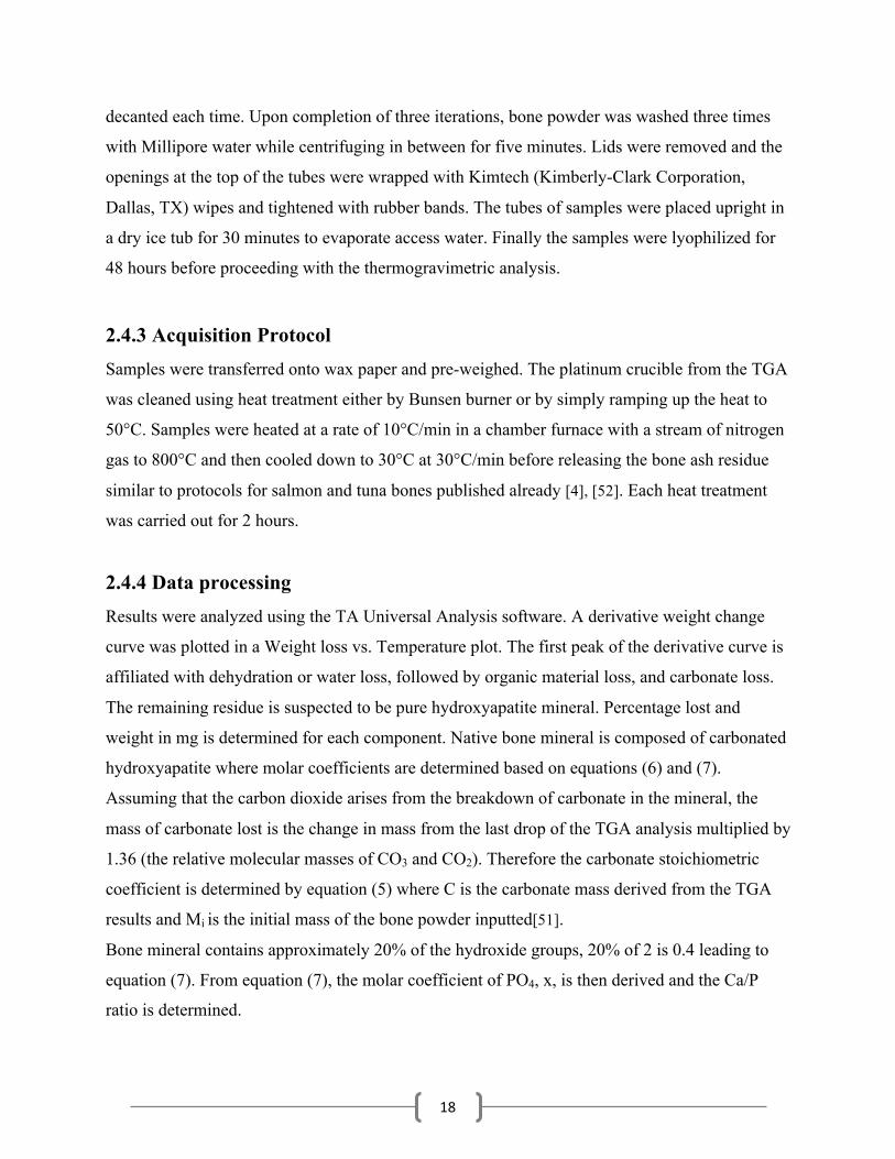
Figure 2-9: About 1-2 mg of bone ash is placed directly onto the sampling stage. A clamp applies pressure to ensure direct contact of sample and crystal. The infrared beam undergoes total internal reflectance and the detector returns a spectrum of absorbance (a.u.) vs. wavelength (cm-1) values.

For this study, ATR-IR first asses samples to have <1% amino acids (confirming the absence of

organic materials). As the IR samples used here have been modified using thermal

decomposition to isolate pure bone apatite, the spectra is expected to resemble one similar to

Hydroxyapatite (second spectra in Figure 2-10). As a result two major peaks, consisting of three

different phosphate vibrations (v1, v3, v4) will be used in this data analysis. Using the raw spectra

data attained from ATR-IR, and these three vibrations in particular, crystal maturity or

crystallinity ratio and crystallinity index is determined upon data processing.

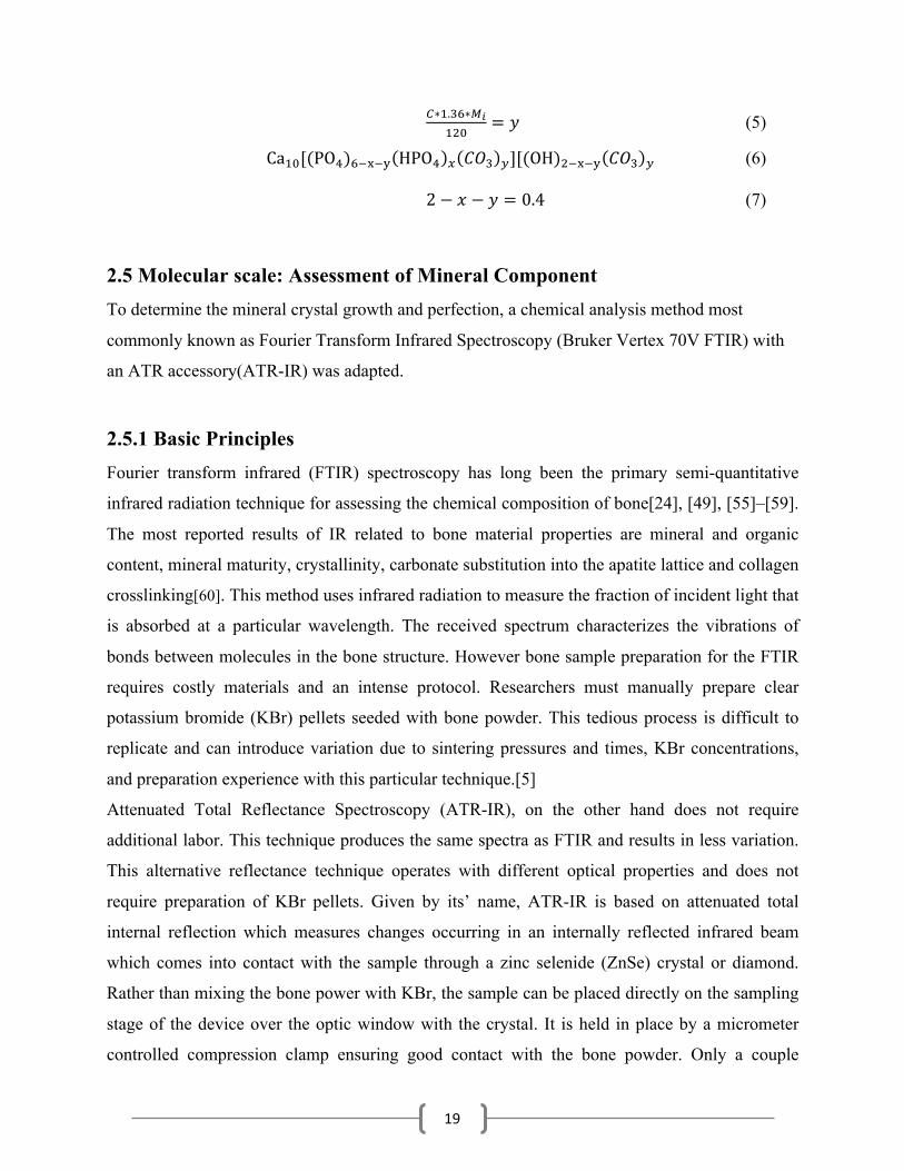
Figure 2-10: Typical IR spectrum of cortical bone its major constituents, hydroxyapatite and collagen spectra shown underneath to model vibrations of most significant bands. (Image adapted from Figueiredo, 2012[60])

21

2.5.2 Sample Preparation

Bone ash retrieved from the thermal analysis was transferred into Eppendorf tubes. No further

sample processing is required for characterizing powder with ATR-IR.

2.5.3 Acquisition Protocol About 1mg of bone ash is loaded directly on the ATR stage. ATR-IR spectra were recorded in

the range of 4000-540 cm-1 under vacuum. In the field of bone, spectrum region of interest is

500-1700cm-1[60]. Interferograms were averaged for 320 scans at 1cm-1 resolution.

2.5.4 Data processing The spectra were obtained and analyzed using Opus (Bruker Optics, Billerica, MA) and Matlab

(See appendix A.3.2, Mathworks, Beltsville, MD). Each bone component has its’ own particular

peak, however often peak widths overlap and spectrum analysis requires additional effort to

characterize individual peaks. The spectrum is first smoothed using Savitzky-Golay’s algorithm

[61]. Overlapping peeks were resolved using a quadratic curved baseline and fitted to a fixed-

width Gaussian function as previously described[62]–[64]. Here two particular calculations of

interest have been derived, the crystallinity index and the mineral maturity (or crystallinity) ratio.

Mineral maturity is determined from sub-bands of the v1 and v3 phosphate vibrations occurring

in the 900-1200 cm-1 region. From deconvolution, two major peaks arise underneath the v1 and

v3 bands, being at 1020 and 1030 cm-1 (Figure 2-11). The sub band at 1020cm-1 is said to be

associated with nonstoichiometric apatite. Meanwhile the sub band at 1030cm-1 is said to be

associated with stoichiometric apatite. Therefore the key to characterizing bone using IR is to

determine the mineral maturity or crystallinity ratio by the 1030/1020 peak area ratio [56], [58].

Crystallinity Index is another parameter that has been found to correlate with the state of

crystallinity of apatite (narrower peak corresponding to higher crystallinity). This parameter is

determined from the inverse of the full width at half maximum (1/FWHM) at the 600cm-1

wavelength band or v4 phosphate vibration [65].

22

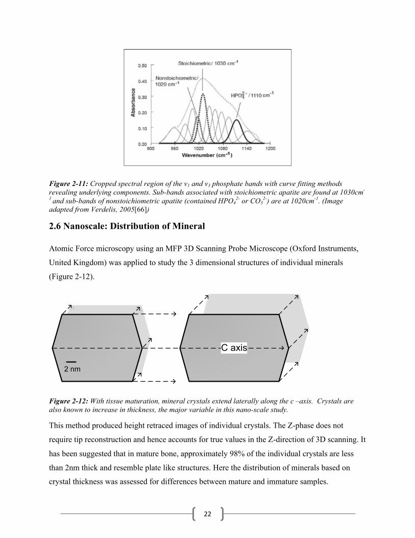
Figure 2-11: Cropped spectral region of the v1 and v3 phosphate bands with curve fitting methods revealing underlying components. Sub-bands associated with stoichiometric apatite are found at 1030cm-

1 and sub-bands of nonstoichiometric apatite (contained HPO42- or CO3

2-) are at 1020cm-1. (Image adapted from Verdelis, 2005[66])

2.6 Nanoscale: Distribution of Mineral

Atomic Force microscopy using an MFP 3D Scanning Probe Microscope (Oxford Instruments,

United Kingdom) was applied to study the 3 dimensional structures of individual minerals

(Figure 2-12).

2 nm

C axis

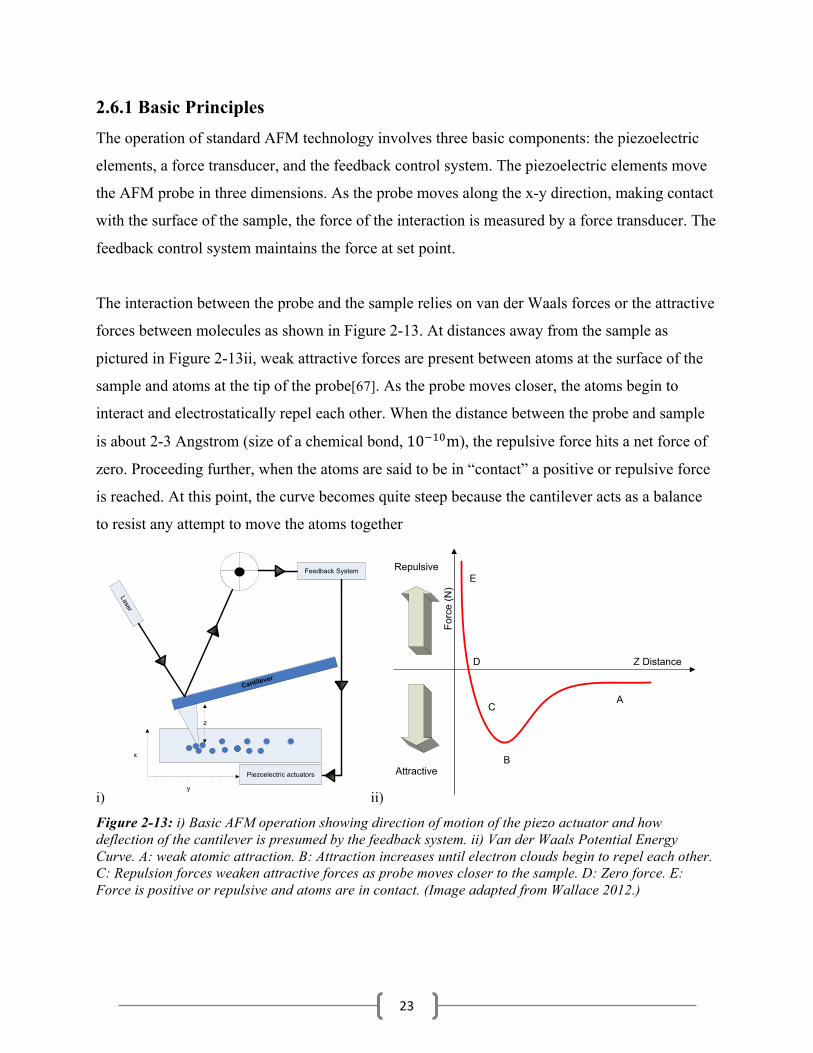
Figure 2-12: With tissue maturation, mineral crystals extend laterally along the c –axis. Crystals are also known to increase in thickness, the major variable in this nano-scale study.

This method produced height retraced images of individual crystals. The Z-phase does not

require tip reconstruction and hence accounts for true values in the Z-direction of 3D scanning. It

has been suggested that in mature bone, approximately 98% of the individual crystals are less

than 2nm thick and resemble plate like structures. Here the distribution of minerals based on

crystal thickness was assessed for differences between mature and immature samples.

23

2.6.1 Basic Principles The operation of standard AFM technology involves three basic components: the piezoelectric

elements, a force transducer, and the feedback control system. The piezoelectric elements move

the AFM probe in three dimensions. As the probe moves along the x-y direction, making contact

with the surface of the sample, the force of the interaction is measured by a force transducer. The

feedback control system maintains the force at set point.

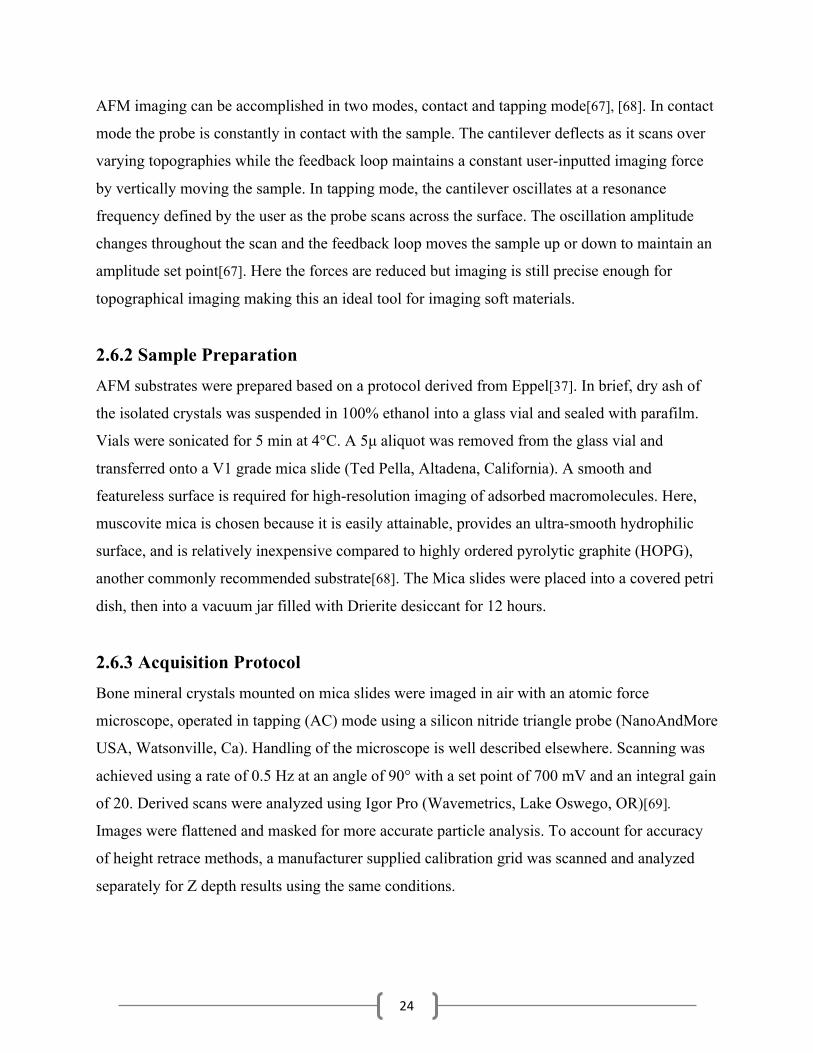
The interaction between the probe and the sample relies on van der Waals forces or the attractive

forces between molecules as shown in Figure 2-13. At distances away from the sample as

pictured in Figure 2-13ii, weak attractive forces are present between atoms at the surface of the

sample and atoms at the tip of the probe[67]. As the probe moves closer, the atoms begin to

interact and electrostatically repel each other. When the distance between the probe and sample

is about 2-3 Angstrom (size of a chemical bond, 10!!"m), the repulsive force hits a net force of

zero. Proceeding further, when the atoms are said to be in “contact” a positive or repulsive force

is reached. At this point, the curve becomes quite steep because the cantilever acts as a balance

to resist any attempt to move the atoms together

i)

Laser

x

y

Feedback System

Piezoelectric actuators

z

Cantilever

ii)

Forc

e (N

)

Z Distance

A

B

C

D

ERepulsive

Attractive

Figure 2-13: i) Basic AFM operation showing direction of motion of the piezo actuator and how deflection of the cantilever is presumed by the feedback system. ii) Van der Waals Potential Energy Curve. A: weak atomic attraction. B: Attraction increases until electron clouds begin to repel each other. C: Repulsion forces weaken attractive forces as probe moves closer to the sample. D: Zero force. E: Force is positive or repulsive and atoms are in contact. (Image adapted from Wallace 2012.)

24

AFM imaging can be accomplished in two modes, contact and tapping mode[67], [68]. In contact

mode the probe is constantly in contact with the sample. The cantilever deflects as it scans over

varying topographies while the feedback loop maintains a constant user-inputted imaging force

by vertically moving the sample. In tapping mode, the cantilever oscillates at a resonance

frequency defined by the user as the probe scans across the surface. The oscillation amplitude

changes throughout the scan and the feedback loop moves the sample up or down to maintain an

amplitude set point[67]. Here the forces are reduced but imaging is still precise enough for

topographical imaging making this an ideal tool for imaging soft materials.

2.6.2 Sample Preparation AFM substrates were prepared based on a protocol derived from Eppel[37]. In brief, dry ash of

the isolated crystals was suspended in 100% ethanol into a glass vial and sealed with parafilm.

Vials were sonicated for 5 min at 4°C. A 5µ aliquot was removed from the glass vial and

transferred onto a V1 grade mica slide (Ted Pella, Altadena, California). A smooth and

featureless surface is required for high-resolution imaging of adsorbed macromolecules. Here,

muscovite mica is chosen because it is easily attainable, provides an ultra-smooth hydrophilic

surface, and is relatively inexpensive compared to highly ordered pyrolytic graphite (HOPG),

another commonly recommended substrate[68]. The Mica slides were placed into a covered petri

dish, then into a vacuum jar filled with Drierite desiccant for 12 hours.

2.6.3 Acquisition Protocol Bone mineral crystals mounted on mica slides were imaged in air with an atomic force

microscope, operated in tapping (AC) mode using a silicon nitride triangle probe (NanoAndMore

USA, Watsonville, Ca). Handling of the microscope is well described elsewhere. Scanning was

achieved using a rate of 0.5 Hz at an angle of 90° with a set point of 700 mV and an integral gain

of 20. Derived scans were analyzed using Igor Pro (Wavemetrics, Lake Oswego, OR)[69].

Images were flattened and masked for more accurate particle analysis. To account for accuracy

of height retrace methods, a manufacturer supplied calibration grid was scanned and analyzed

separately for Z depth results using the same conditions.

25

2.7 Statistical Analysis

Mean values and standard deviations were calculated for the measured parameters. Distribution

of data was determined using a Shapiro-Wilke test. Parametric t-test was performed on normally

distributed data and non-parametric t-tests were performed on normally distributed data.

Independent t-tests were used to compare geometrical properties, compositional properties, and

micro-mechanical parameters such as yield stress (𝜎𝑦𝑖𝑒𝑙𝑑), ultimate stress (σmax), and total work

(Wt). Welch’s t-test was performed on remaining micro-mechanical properties including elastic

modulus (E), strain (𝜀𝑦𝑖𝑒𝑙𝑑), strain (εmax), elastic work (We), and plastic work (Wp). No statistical

analysis was performed on nano-scale crystal assessment due to the small sample size. Equality

of variances was assumed when Levene’s Test gave values of p > 0.05. Mann-Whitney U test

was used in the cases where the data was not normally distributed according to the Shapiro-Wilk

test. Differences were considered significant at p < 0.05. Statistical analysis was performed using

SPSS (v.21, SPSS Inc., Chicago, IL).

26

3 Results This chapter presents the results attained from this study. Results from each step of the protocol

are described in consecutive subchapters. The geometrical data derived from the µCt is presented

first. These results were then used for mechanical testing of bone, proceeding with compositional

and chemical analysis. Lastly 3D imaging data is presented to assess mineral distribution based

on crystal thickness as a determinant of strength of the collagen-mineral interface (TC-cAP).

Results are herein described in international standard units and in terms of exact values or means

(±standard deviation).

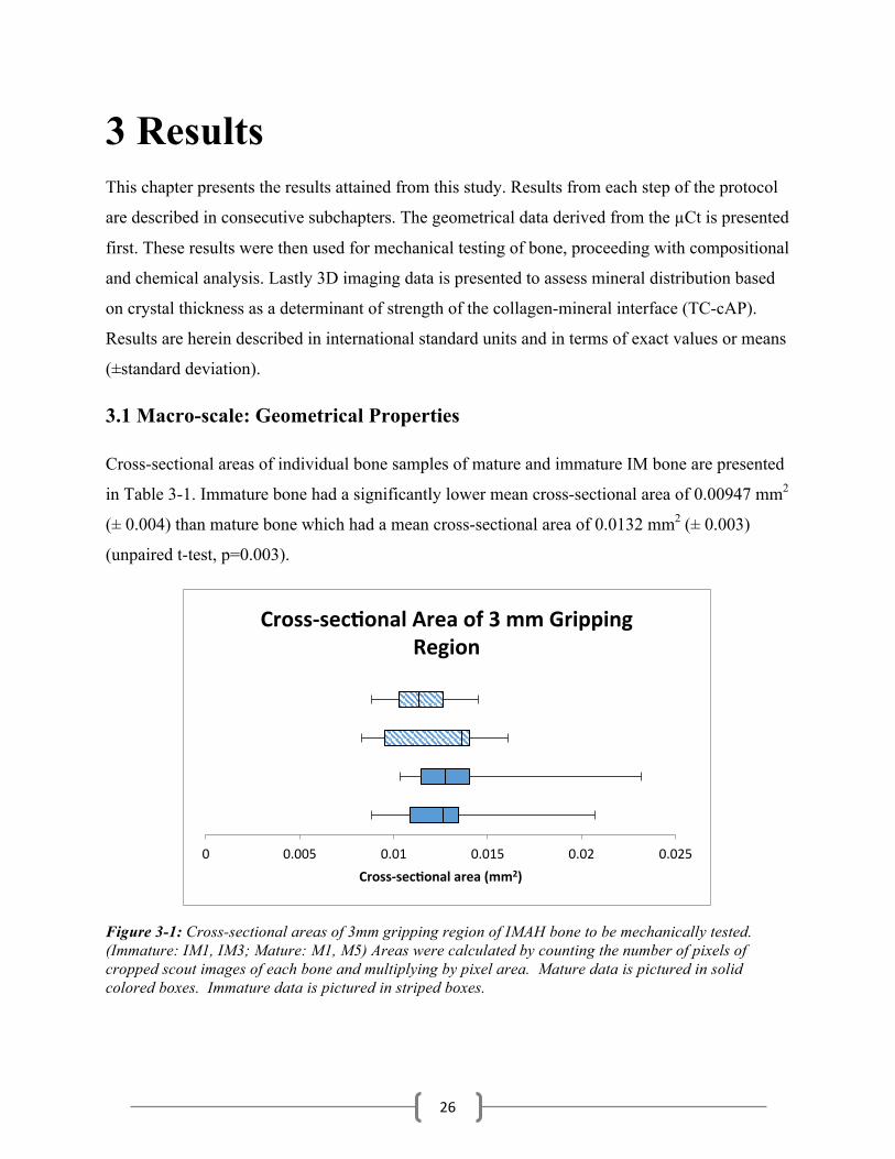
3.1 Macro-scale: Geometrical Properties

Cross-sectional areas of individual bone samples of mature and immature IM bone are presented

in Table 3-1. Immature bone had a significantly lower mean cross-sectional area of 0.00947 mm2

(± 0.004) than mature bone which had a mean cross-sectional area of 0.0132 mm2 (± 0.003)

(unpaired t-test, p=0.003).

Figure 3-1: Cross-sectional areas of 3mm gripping region of IMAH bone to be mechanically tested. (Immature: IM1, IM3; Mature: M1, M5) Areas were calculated by counting the number of pixels of cropped scout images of each bone and multiplying by pixel area. Mature data is pictured in solid colored boxes. Immature data is pictured in striped boxes.

0 0.005 0.01 0.015 0.02 0.025Cross-sec?onalarea(mm2)

Cross-sec?onalAreaof3mmGrippingRegion

27

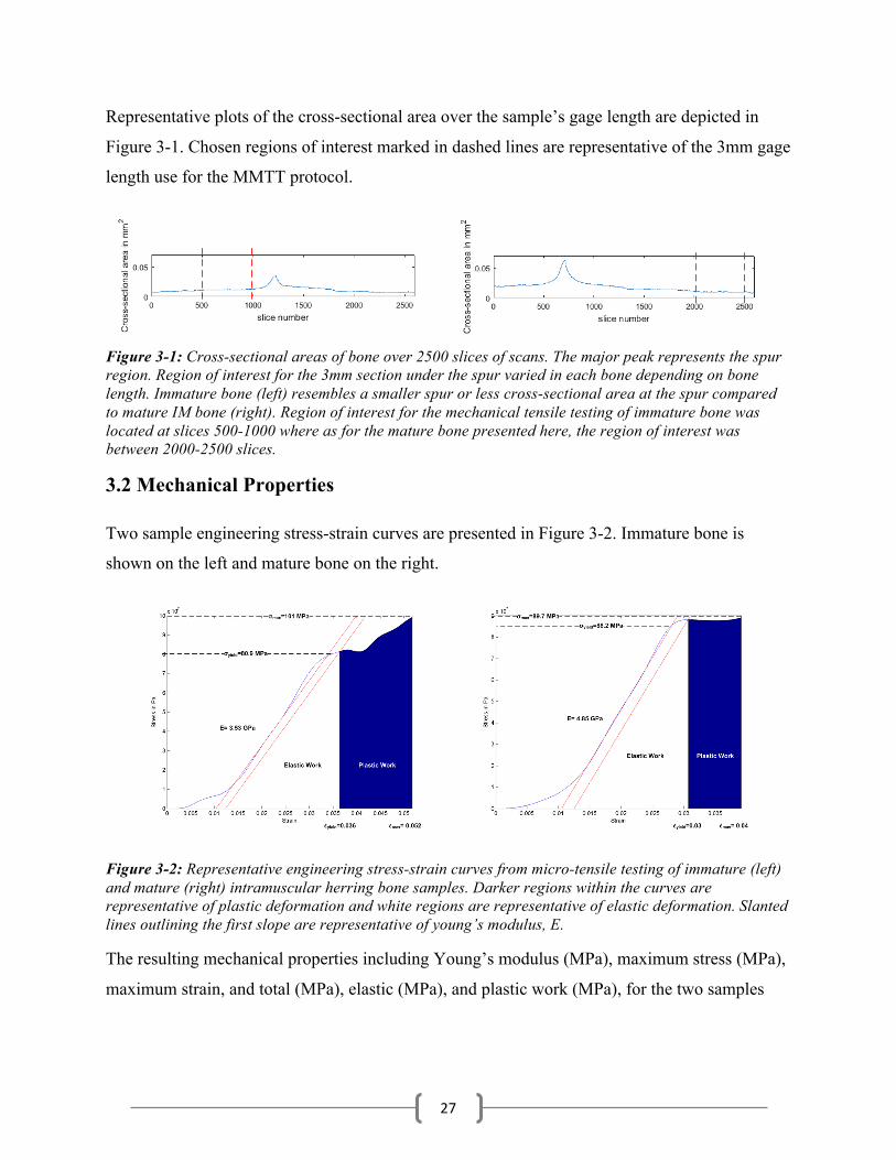
Representative plots of the cross-sectional area over the sample’s gage length are depicted in

Figure 3-1. Chosen regions of interest marked in dashed lines are representative of the 3mm gage

length use for the MMTT protocol.

Figure 3-1: Cross-sectional areas of bone over 2500 slices of scans. The major peak represents the spur region. Region of interest for the 3mm section under the spur varied in each bone depending on bone length. Immature bone (left) resembles a smaller spur or less cross-sectional area at the spur compared to mature IM bone (right). Region of interest for the mechanical tensile testing of immature bone was located at slices 500-1000 where as for the mature bone presented here, the region of interest was between 2000-2500 slices.

3.2 Mechanical Properties

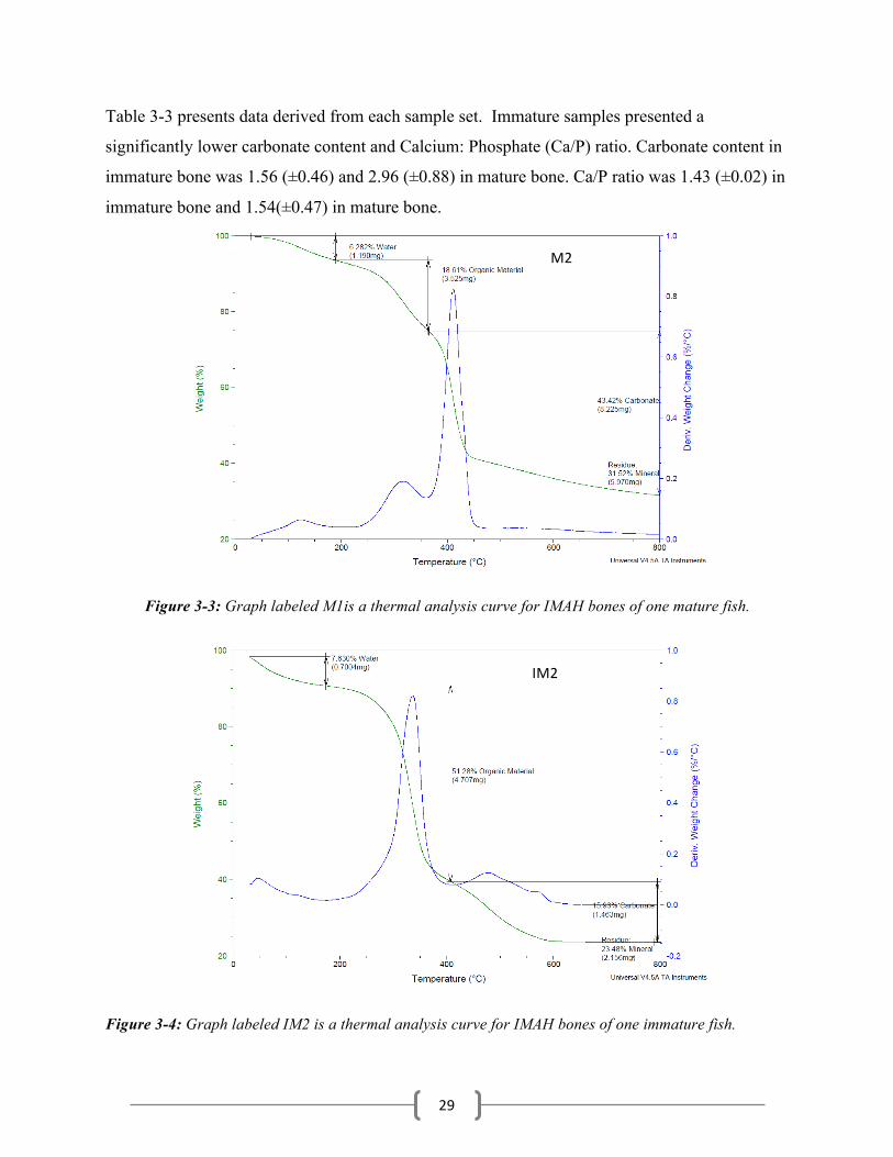
Two sample engineering stress-strain curves are presented in Figure 3-2. Immature bone is

shown on the left and mature bone on the right.

Figure 3-2: Representative engineering stress-strain curves from micro-tensile testing of immature (left) and mature (right) intramuscular herring bone samples. Darker regions within the curves are representative of plastic deformation and white regions are representative of elastic deformation. Slanted lines outlining the first slope are representative of young’s modulus, E.

The resulting mechanical properties including Young’s modulus (MPa), maximum stress (MPa),

maximum strain, and total (MPa), elastic (MPa), and plastic work (MPa), for the two samples

28

above are listed in Table 3-2. Parameters for all IM bones tested in this study can be found in the

appendix (A.1.1.1 and A.1.2.1).

Young’s modulus was significantly higher in mature IM bone than in immature IM bone by 60%

(p = 0.013, unpaired t-test). Although not significant, indicative comparison showed that yield

stress was 18 percent higher in mature IM bone than in immature IM bones (p = 0.358, unpaired

t-test). Likewise, maximum stress was 40 percent higher in mature IM bone at than in immature

IM bone (p = 0.387, unpaired t-test).

Although not significantly different, indicative comparison showed that yield strain was 25%

lower in mature bone than in mature bone (p=0.157, unpaired t-test). Maximum strain, although

not significant, was 12% lower in mature bone than immature bone (p=0.157, unpaired t-test).

Elastic work was not significantly different in mature and immature samples (p = 0.761, unpaired

t-test). Plastic work was not significantly different either (p = 0.702, independent t-test). In

addition total work was not significantly different in mature and immature IM bone (independent

t-test, p=0.808).

Immature: IM1 (N=12)

Mature: M1 (N=9)

Indicative Comparison

Young’s Modulus, E (GPa)* 3.29 (±1.97) 5.26 (±1.44) 1.60 Yield strain, εyield 0.03 (±0.01) 0.02 (±0.01) 0.75

Yield stress, σyield (MPa) 61.5 (±24.5) 72.8 (±17.9) 1.18 Maximum stress, σmax (MPa) 106 (±42.4) 150 (±37.7) 1.40

Maximum strain, εmax 0.08 (±0.02) 0.07 (±0.05) 0.88 Elastic work, We (MPa) 0.77 (±0.35) 0.73 (±0.03) 0.94 Plastic work, Wp (MPa) 4.13 (±3.22) 4.23 (±4.85) 1.02 Total work, Wt (MPa) 4.90 (±3.32) 4.96 (±4.88) 1.01

Table 3-2: Results of micromechanical tensile testing of intra-muscular Herring fish bone from immature and mature samples. Significant differences between groups were assessed with independent t-tests at a significance level of 0.05. *p<0.05

3.3 Macro scale: Compositional Analysis

Figures 3-3 and 3-4 are thermal analysis curves derived during the isolation of the mineral

component of one example of immature and mature IMAH bone, respectively.

29

Table 3-3 presents data derived from each sample set. Immature samples presented a

significantly lower carbonate content and Calcium: Phosphate (Ca/P) ratio. Carbonate content in

immature bone was 1.56 (±0.46) and 2.96 (±0.88) in mature bone. Ca/P ratio was 1.43 (±0.02) in

immature bone and 1.54(±0.47) in mature bone.

Figure 3-3: Graph labeled M1is a thermal analysis curve for IMAH bones of one mature fish.

Figure 3-4: Graph labeled IM2 is a thermal analysis curve for IMAH bones of one immature fish.

M2

IM2

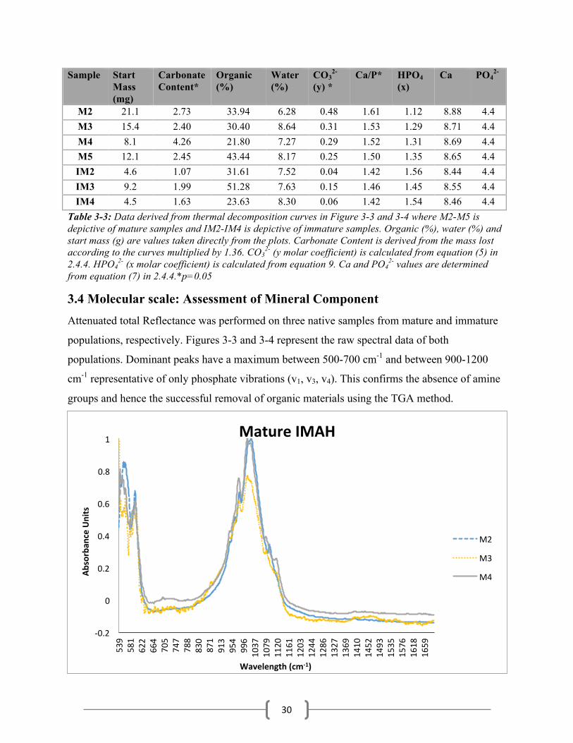
30

Sample Start Mass (mg)

Carbonate Content*

Organic (%)

Water (%)

CO32-

(y) * Ca/P* HPO4

(x) Ca PO4

2-

M2 21.1 2.73 33.94 6.28 0.48 1.61 1.12 8.88 4.4 M3 15.4 2.40 30.40 8.64 0.31 1.53 1.29 8.71 4.4 M4 8.1 4.26 21.80 7.27 0.29 1.52 1.31 8.69 4.4 M5 12.1 2.45 43.44 8.17 0.25 1.50 1.35 8.65 4.4 IM2 4.6 1.07 31.61 7.52 0.04 1.42 1.56 8.44 4.4 IM3 9.2 1.99 51.28 7.63 0.15 1.46 1.45 8.55 4.4 IM4 4.5 1.63 23.63 8.30 0.06 1.42 1.54 8.46 4.4

Table 3-3: Data derived from thermal decomposition curves in Figure 3-3 and 3-4 where M2-M5 is depictive of mature samples and IM2-IM4 is depictive of immature samples. Organic (%), water (%) and start mass (g) are values taken directly from the plots. Carbonate Content is derived from the mass lost according to the curves multiplied by 1.36. CO3

2- (y molar coefficient) is calculated from equation (5) in 2.4.4. HPO4

2- (x molar coefficient) is calculated from equation 9. Ca and PO42- values are determined

from equation (7) in 2.4.4.*p=0.05

3.4 Molecular scale: Assessment of Mineral Component Attenuated total Reflectance was performed on three native samples from mature and immature

populations, respectively. Figures 3-3 and 3-4 represent the raw spectral data of both

populations. Dominant peaks have a maximum between 500-700 cm-1 and between 900-1200

cm-1 representative of only phosphate vibrations (v1, v3, v4). This confirms the absence of amine

groups and hence the successful removal of organic materials using the TGA method.

-0.2

0

0.2

0.4

0.6

0.8

1

539

581

622

664

705

747

788

830

871

913

954

996

1037

1079

1120

1161

1203

1244

1286

1327

1369

1410

1452

1493

1535

1576

1618

1659

Absorban

ceUnits

Wavelength(cm-1)

MatureIMAH

M2

M3

M4

31

Figures 3-3: Normalized ATR-IR spectra of three mature herring bone samples.

.Figures 3-4: Normalized ATR-IR spectra of immature herring bone samples.

Crystallinity ratio and crystallinity index are presented in Table 3-3. Mature samples presented

an average crystallinity ratio of 0.214 (±0.19) and crystallinity index of 0.014 (±0.09). Immature

samples presented a mean crystallinity ratio of 2.94 (±1.50) and crystallinity index of 0.013

(±0.01). The crystallinity ratio of mature IMAH bone was significantly higher than that of the

immature IMAH bone as per a non-parametric t-test. The crystallinity index is not statistically

different amongst populations.

Sample Crystallinity ratio*

Crystallinity Index

M2 0.092 0.010 M3 0.109 0.008 M4 0.441 0.024 IM2 2.820 0.011 IM3 4.500 0.024 IM4 1.514 0.005

-0.2

0

0.2

0.4

0.6

0.8

1539

581

622

664

705

747

788

830

871

913

954

996

1037

1079

1120

1161

1203

1244

1286

1327

1369

1410

1452

1493

1535

1576

1618

1659

Absorban

ceUnits

Wavelength(cm-1)

ImmatureIMAH

IM2

IM3

IM4

32

Table 3-3: Crystallinity ratio and index of mature samples (M2-M4) and immature sample (IM2-IM4). (*P=0.05, independent t-test)

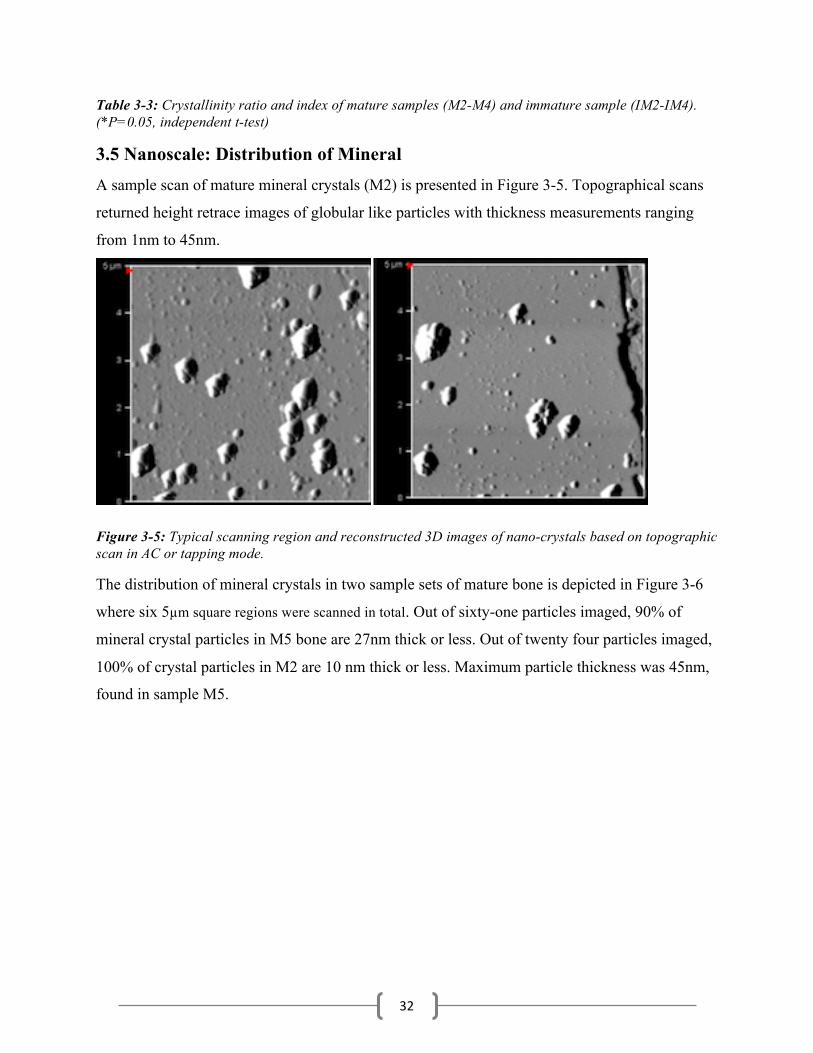
3.5 Nanoscale: Distribution of Mineral A sample scan of mature mineral crystals (M2) is presented in Figure 3-5. Topographical scans

returned height retrace images of globular like particles with thickness measurements ranging

from 1nm to 45nm.

Figure 3-5: Typical scanning region and reconstructed 3D images of nano-crystals based on topographic scan in AC or tapping mode.

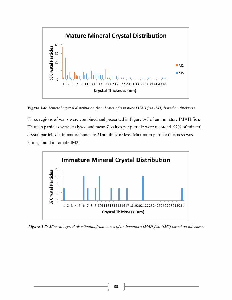
The distribution of mineral crystals in two sample sets of mature bone is depicted in Figure 3-6

where six 5µm square regions were scanned in total. Out of sixty-one particles imaged, 90% of

mineral crystal particles in M5 bone are 27nm thick or less. Out of twenty four particles imaged,

100% of crystal particles in M2 are 10 nm thick or less. Maximum particle thickness was 45nm,

found in sample M5.

33

Figure 3-6: Mineral crystal distribution from bones of a mature IMAH fish (M5) based on thickness.

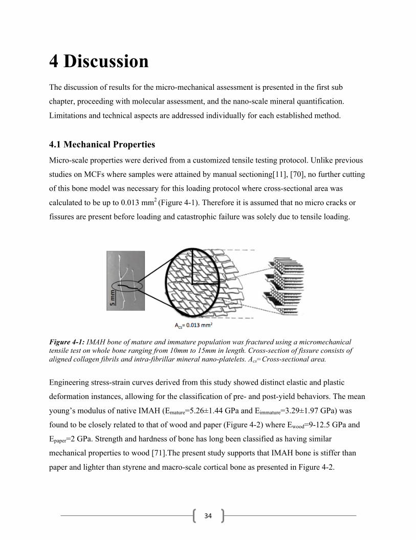
Three regions of scans were combined and presented in Figure 3-7 of an immature IMAH fish.

Thirteen particles were analyzed and mean Z values per particle were recorded. 92% of mineral

crystal particles in immature bone are 21nm thick or less. Maximum particle thickness was

31nm, found in sample IM2.

Figure 3-7: Mineral crystal distribution from bones of an immature IMAH fish (IM2) based on thickness.

0

10

20

30

40

1 3 5 7 9 111315171921232527293133353739414345

%CrystalPar?cles

CrystalThickness(nm)

MatureMineralCrystalDistribu?on

M2

M5

0

5

10

15

20

1 2 3 4 5 6 7 8 910111213141516171819202122232425262728293031%CrystalPar?cles

CrystalThickness(nm)

ImmatureMineralCrystalDistribu?on

34

4 Discussion The discussion of results for the micro-mechanical assessment is presented in the first sub

chapter, proceeding with molecular assessment, and the nano-scale mineral quantification.

Limitations and technical aspects are addressed individually for each established method.

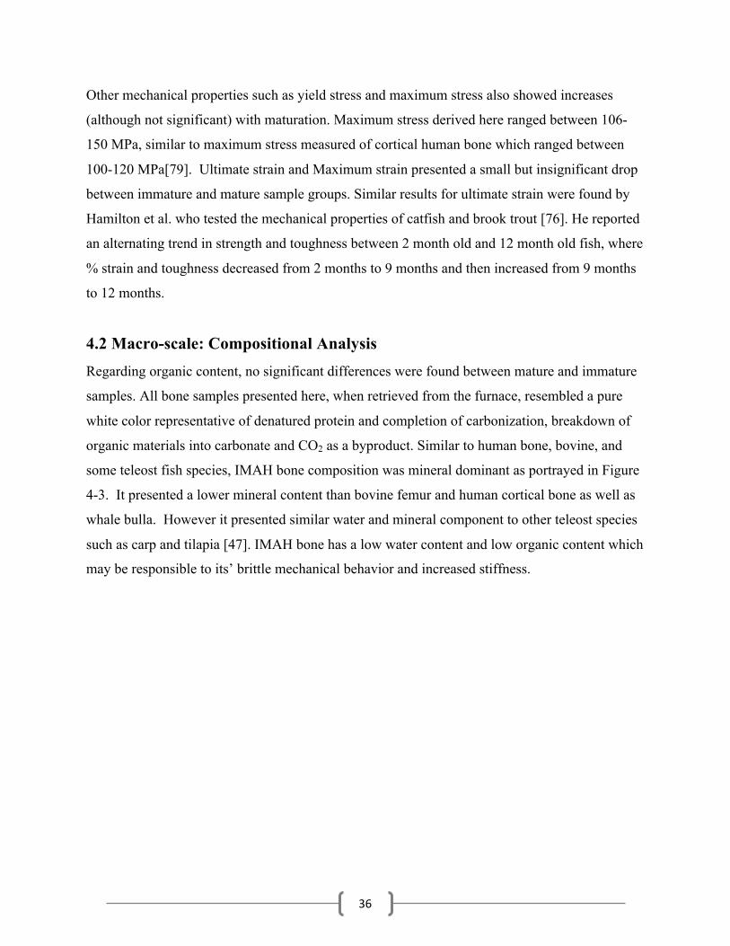
4.1 Mechanical Properties Micro-scale properties were derived from a customized tensile testing protocol. Unlike previous

studies on MCFs where samples were attained by manual sectioning[11], [70], no further cutting

of this bone model was necessary for this loading protocol where cross-sectional area was

calculated to be up to 0.013 mm2 (Figure 4-1). Therefore it is assumed that no micro cracks or

fissures are present before loading and catastrophic failure was solely due to tensile loading.

Figure 4-1: IMAH bone of mature and immature population was fractured using a micromechanical tensile test on whole bone ranging from 10mm to 15mm in length. Cross-section of fissure consists of aligned collagen fibrils and intra-fibrillar mineral nano-platelets. Acs=Cross-sectional area.

Engineering stress-strain curves derived from this study showed distinct elastic and plastic

deformation instances, allowing for the classification of pre- and post-yield behaviors. The mean

young’s modulus of native IMAH (Emature=5.26±1.44 GPa and Eimmature=3.29±1.97 GPa) was

found to be closely related to that of wood and paper (Figure 4-2) where Ewood=9-12.5 GPa and

Epaper=2 GPa. Strength and hardness of bone has long been classified as having similar

mechanical properties to wood [71].The present study supports that IMAH bone is stiffer than

paper and lighter than styrene and macro-scale cortical bone as presented in Figure 4-2.

35

You

ng’s

Mod

ulus

(E)

Density (g/cm3)

S

Wood

P

CB

IMAH5

10

15

20

25

0.80.4 1.2 1.6 2

Figure 4-2: Ashby plot of stiffness for various known materials and their relation to the sample of interest in this study. E for IMAH is based on average values calculated from Table 3.1. Mass density of IMAH bone was determined using Archimedes’ principle. The Young’s modulus presented here for styrene(S), wood(W), compact bone(CB), and paper(P) is a combination of calculated and known values. Ewood=9-14.9 GPa, Epaper=2-4 GPa,, Estyrene=2.9-3.5 GPa[72]–[75].

Immature bone of IMAH exhibited a polymer like behavior post yield. This weakening behavior

may be due to the reduced mineral content in immature samples. The tensile modulus of cortical

bone in mammalians has been shown to have E values between 13 and 25 GPa. However, recent

micro-mechanical tests on low mineralized MCFs from deer antler reported values of 1 GPa and

5 GPa, rather close to the intra-fibrillarly mineralized bone tested here[76], [77]. In addition,

another study using an atomic force microscope mounted onto a scanning electron microscope,

did a micro-scale tensile test and determined the moduli of intra-fibrillarly mineralized collagen

fibrils to be around 2 GPa[11]. Similarly to findings from this mechanical assessment, previous

studies reported that E values of child fibulas were significantly lower than adult fibulas[78].

Therefore stiffness indeed increases with developing bone.

36

Other mechanical properties such as yield stress and maximum stress also showed increases

(although not significant) with maturation. Maximum stress derived here ranged between 106-

150 MPa, similar to maximum stress measured of cortical human bone which ranged between

100-120 MPa[79]. Ultimate strain and Maximum strain presented a small but insignificant drop

between immature and mature sample groups. Similar results for ultimate strain were found by

Hamilton et al. who tested the mechanical properties of catfish and brook trout [76]. He reported

an alternating trend in strength and toughness between 2 month old and 12 month old fish, where

% strain and toughness decreased from 2 months to 9 months and then increased from 9 months

to 12 months.

4.2 Macro-scale: Compositional Analysis Regarding organic content, no significant differences were found between mature and immature

samples. All bone samples presented here, when retrieved from the furnace, resembled a pure

white color representative of denatured protein and completion of carbonization, breakdown of

organic materials into carbonate and CO2 as a byproduct. Similar to human bone, bovine, and

some teleost fish species, IMAH bone composition was mineral dominant as portrayed in Figure

4-3. It presented a lower mineral content than bovine femur and human cortical bone as well as

whale bulla. However it presented similar water and mineral component to other teleost species

such as carp and tilapia [47]. IMAH bone has a low water content and low organic content which

may be responsible to its’ brittle mechanical behavior and increased stiffness.

37

100% Mineral

100% Water 100% OrganicOrganic

Whale bulla

Bovine femur

IMAH

Carp

Human iIiac crest

Tilapia

Cod

Water Dominant Organic Material Dominant

Mineral Dominant

Shark vertebrae

Batoid propterygia

Articular cartilage

Mineral

Wat

er

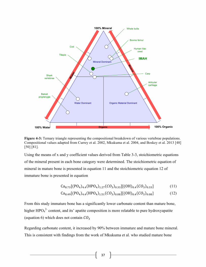
Figure 4-3: Ternary triangle representing the compositional breakdown of various vertebrae populations. Compositional values adapted from Currey et al. 2002, Mkukuma et al. 2004, and Boskey et al. 2013 [48] [50] [81].

Using the means of x and y coefficient values derived from Table 3-3, stoichiometric equations

of the mineral present in each bone category were determined. The stoichiometric equation of

mineral in mature bone is presented in equation 11 and the stoichiometric equation 12 of

immature bone is presented in equation

Ca!.!"[(PO!)!.! HPO! !.!" 𝐶𝑂! !.!!][(OH)!.! 𝐶𝑂! !.!!] (11)

Ca!.!"[(PO!)!.! HPO! !.!" 𝐶𝑂! !.!"][(OH)!.! 𝐶𝑂! !.!"] (12)

From this study immature bone has a significantly lower carbonate content than mature bone,

higher HPO42- content, and its’ apatite composition is more relatable to pure hydroxyapatite

(equation 6) which does not contain 𝐶𝑂!

Regarding carbonate content, it increased by 90% between immature and mature bone mineral.

This is consistent with findings from the work of Mkukuma et al. who studied mature bone

38

mineral of whale bone and immature bone mineral of deer antler[51]. Decomposition of mineral

can produce β-Tricalcium phosphate (TCP) and hydroxyapatite (HAP) in immature bone

mineral. Meanwhile mature bone mineral decomposes to calcium oxide (CaO) and HAP. TCP is

associated with calcium deficiency and an increased HPO42- presence[2], [51]. According to

Table 3-3, it appears that bone samples used here are calcium-deficient (Ca/P <1.67) apatite.

This expected as the IMAH bone used here is intra-fibrillar and indicative of only the early

stages of maturation. From this study and several previous studies, it was shown that immature

bone has a low mineral content and contains mineral that is high in PO42- and low in CO3

2-. [52],

[78]–[80].

The higher mineral content in mature bone may be responsible for the stiffening effect presented

in 4.1. Another study by Pellegrino and Blitz reported a positive correlation between Ca/P molar

ratio and the carbonate content by using immature rabbit and mature turtle bone[85]. The Ca/P

ratio is a sensitive measure of bone mineral changes[86], [87]. Given that results presented here

depict increasing Ca/P ratio and carbonate with maturation, this study supports the increase of

mineral content within developing bone tissue.

4.3 Molecular scale: Assessment of Mineral Component ATR-IR spectra successfully demonstrated the absence of collagen in all samples. There appear

to be no sharp bands at 1634, 1410, 1445, and 1548 cm-1, avoiding the presence of organic

materials due to successful deproteinization from the TGA protocol. Regarding crystallinity

ratio, the ratio of stoichiometric apatite to nonstoichiometric apatite, it decreased with mineral

maturation. Similarly, Miller et al. [88] tested bone quality in developing mice using tibia bone

and discovered that 1020/1030 cm-1 ratio increases with increasing stiffness (E tested using

nano-indentation) [88]. Yet here its inverse, the 1030/1020 cm-1 ratio, more commonly referred

to crystallinity ratio is adapted [52], [82]–[84].

Therefore it supports that the decrease in crystallinity ratio found here may be correlated with an

increase in E. In addition, non-stoichiometric apatite contains HPO42- and CO3

2- as depicted in

3.2 which suggests why crystallinity ratio may have decreased in mature bone samples. In 4.1,

mature samples presented a higher HPO42- and CO3

2- content and therefore depict more non-

stoichiometric apatite present in the tissue compared to stoichiometric apatite.

39

Regarding the crystallinity index of IMAH bone, no significant differences were reported in the

two populations. In addition, the crystallinity index of mouse femur retrieved from this protocol

was 0.014, identical to the adult IMAH population. This insignificance may have resulted from

the absence of a well-defined peak at a wavelength of 600cm-1 in some samples (see IM2).

Additionally, crystallinity index is a measure most commonly reported from X-ray diffraction

and therefore the IR band may have not been as well resolved as one derived from other

techniques. It has also been reported that mineral maturity and crystallinity index present a

strong correlation only in synthetic apatite but may be poorly correlated in native apatite which

could explain why crystallinity ratio decreased significantly amongst populations meanwhile the

crystallinity index remained stagnant[60].

IR spectra are composed of several overlapping peaks, so after deconvolution and curve fitting

methods, results are reported as a percentage of the areas of specific bands. Therefore, IR data

may be primarily used for comparison purposes rather than absolute.

Another measure of maturity of the mineral phase is the carbonate to phosphate ratio. Because

carbonate was removed during the process of calcination, it was not feasible to measure it in this

study. However, as mentioned in 3.2, the amount of substitutions within the crystal lattice

structure, carbonate being the dominant one, could be an indicator of apatite quality. For future

work, it may be interesting to run an IR spectrum on whole bone before calcination to compare

and be able to reduce spectra based on raw bone and thermally treated bone.

The molecular assessment of this study agreed with the previous compositional analysis in terms

of increased carbonate substitution with maturation and showed a significant difference in

mineral maturity of aging tissue, measured by the crystallinity ratio.

4.4 Nanoscale: Distribution of Mineral Mineral crystal thickness varied with maturity. The maximum thickness of mineral crystals in

mature bone was 6 nm higher than that of immature bone. Due to small sample size, statistical

analysis was not feasible.

Previous studies have successfully imaged intact trabecular bone of bovine and calvarias of rats

using AFM. These techniques showed a very close interaction between collagen fibrils and

mineral crystals, where mineral crystals pack like fish scales on the fibrils. They show a densely

woven structure of collagen fibrils, aligned with a 67-nm periodicity and tightly seeded with

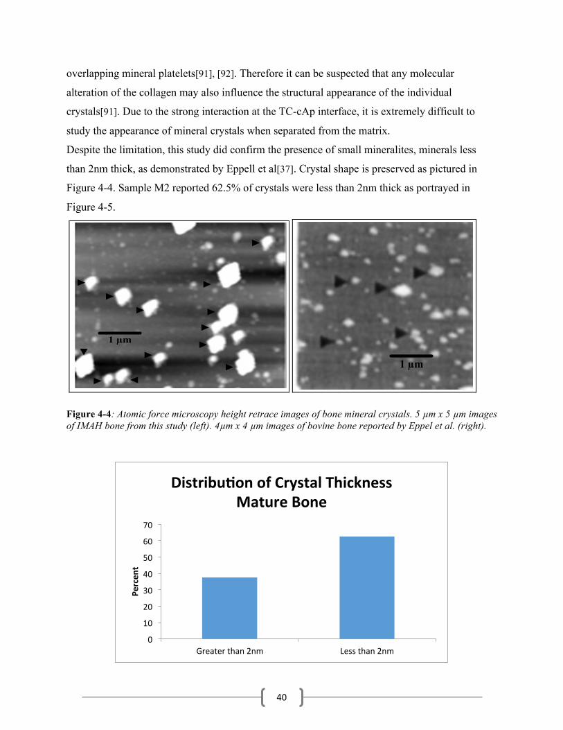
40

overlapping mineral platelets[91], [92]. Therefore it can be suspected that any molecular

alteration of the collagen may also influence the structural appearance of the individual

crystals[91]. Due to the strong interaction at the TC-cAp interface, it is extremely difficult to

study the appearance of mineral crystals when separated from the matrix.

Despite the limitation, this study did confirm the presence of small mineralites, minerals less

than 2nm thick, as demonstrated by Eppell et al[37]. Crystal shape is preserved as pictured in

Figure 4-4. Sample M2 reported 62.5% of crystals were less than 2nm thick as portrayed in

Figure 4-5.

1 µm

►►►

►

►

►►

►►

►

►

►

►

1 µm

Figure 4-4: Atomic force microscopy height retrace images of bone mineral crystals. 5 µm x 5 µm images of IMAH bone from this study (left). 4µm x 4 µm images of bovine bone reported by Eppel et al. (right).

0

10

20

30

40

50

60

70

Greaterthan2nm Lessthan2nm

Percen

t

Distribu?onofCrystalThicknessMatureBone

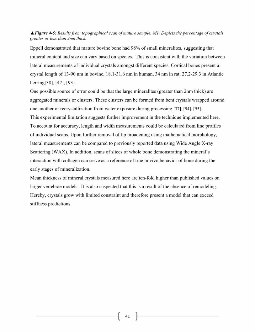
41

▲Figure 4-5: Results from topographical scan of mature sample, M1. Depicts the percentage of crystals greater or less than 2nm thick.

Eppell demonstrated that mature bovine bone had 98% of small mineralites, suggesting that

mineral content and size can vary based on species. This is consistent with the variation between

lateral measurements of individual crystals amongst different species. Cortical bones present a

crystal length of 13-90 nm in bovine, 18.1-31.6 nm in human, 34 nm in rat, 27.2-29.3 in Atlantic

herring[38], [47], [93].

One possible source of error could be that the large mineralites (greater than 2nm thick) are

aggregated minerals or clusters. These clusters can be formed from bent crystals wrapped around

one another or recrystallization from water exposure during processing [37], [94], [95].

This experimental limitation suggests further improvement in the technique implemented here.

To account for accuracy, length and width measurements could be calculated from line profiles

of individual scans. Upon further removal of tip broadening using mathematical morphology,

lateral measurements can be compared to previously reported data using Wide Angle X-ray

Scattering (WAX). In addition, scans of slices of whole bone demonstrating the mineral’s

interaction with collagen can serve as a reference of true in vivo behavior of bone during the

early stages of mineralization.

Mean thickness of mineral crystals measured here are ten-fold higher than published values on

larger vertebrae models. It is also suspected that this is a result of the absence of remodeling.

Hereby, crystals grow with limited constraint and therefore present a model that can exceed

stiffness predictions.

42

5 Conclusion This multiscale characterization of bone tissue aimed at assessing the link between mineral-

related properties and micro-mechanical tensile properties. An experimental set-up consisting of

mechanical, compositional, and structural tissue characterization was developed and dedicated to

investigating the intramuscular bones of the Atlantic herring fish. Previous studies have proposed

this to be a unique model for the basic structure of bone[43], [96]. Given the low stiffness, high

plastic deformation and small crystal size of native bones, together with previously described

intra-fibrillar mineral deposition, present samples were found to be suitable for representing

early stage mineralization of human bone.

Here mechanical and mineral-related properties of intramuscular fish bones were compared at

two different stages of maturation where tissue age was assumed to correspond with sample age.

Hereby, bone tissue from mature fish was found to be stiffer than from immature fish. For the

first time, the compositional investigations of IMAH have shown that carbonate content, calcium

phosphate ratio, and crystallinity ratio increased with maturation while crystallinity index was

not subjected to any changes. Micro tensile tests established within this study revealed light,

stiff, and tough biomaterial properties within all IMAH samples. Compositional structure

analysis of IMAH bone revealed a low density, less mineralized composite than other

mammalian bone models. This supports IMAH bone to be an effective model of early stages of

maturation. Crystal thickness was calculated from topographical atomic force microscopy scans

and demonstrated that crystal thickness increases with maturation stages as well.

Compositional, chemical, and structural changes of the mineral crystal are responsible for the

stiffness and toughness of bone tissue. As a result, cAp growth at the TC-cAp interface may

result in more molecular interactions, collagen distortion, and mechanical interlocking. Further

analysis of this type of bonding may be the key to developing synthetic bone grafts that are light

weight and can withstand critical loads.

43

6 References [1] B.Depalle,Z.Qin,S.J.Shefelbine,andM.J.Buehler,“LargeDeformationMechanisms,Plasticity,

andFailureofanIndividualCollagenFibrilWithDifferentMineralContent,”J.BoneMiner.Res.,vol.31,no.2,pp.380–390,Feb.2016.

[2] N.Rodriguez-Florezetal.,“Aninvestigationofthemineralinductileandbrittlecorticalmousebone,”J.BoneMiner.Res.Off.J.Am.Soc.BoneMiner.Res.,vol.30,no.5,pp.786–795,May2015.

[3] A.Gautieri,A.K.Nair,M.J.Buehler,andS.-W.Chang,“Molecularmechanicsofmineralizedcollagenfibrilsinbone,”Nat.Commun.,vol.4,p.1724,Apr.2013.

[4] J.Venkatesan,Z.J.Qian,B.Ryu,N.V.Thomas,andS.K.Kim,“AcomparativestudyofthermalcalcinationandanalkalinehydrolysismethodintheisolationofhydroxyapatitefromThunnusobesusbone,”Biomed.Mater.BristolEngl.,vol.6,no.3,p.035003,Jun.2011.

[5] S.R.Stock,“TheMineral–CollagenInterfaceinBone,”Calcif.TissueInt.,vol.97,no.3,pp.262–280,Sep.2015.

[6] “DoITPoMS-TLPLibraryStructureofboneandimplantmaterials-Mechanicalpropertiesofbone.”[Online].Available:https://www.doitpoms.ac.uk/tlplib/bones/bone_mechanical.php.[Accessed:29-Nov-2017].

[7] M.Debras,“Contributionofbone’sbiologicalcomponentstoitsmechanicalbehavior,”CollegeofStatenIsland,Sep.2017.

[8] N.Reznikov,R.Shahar,andS.Weiner,“Bonehierarchicalstructureinthreedimensions,”ActaBiomater.,vol.10,no.9,pp.3815–3826,Sep.2014.

[9] J.-Y.Rho,L.Kuhn-Spearing,andP.Zioupos,“Mechanicalpropertiesandthehierarchicalstructureofbone,”Med.Eng.Phys.,vol.20,no.2,pp.92–102,Mar.1998.

[10] I.JägerandP.Fratzl,“Mineralizedcollagenfibrils:amechanicalmodelwithastaggeredarrangementofmineralparticles,”Biophys.J.,vol.79,no.4,pp.1737–1746,Oct.2000.

[11] F.HangandA.H.Barber,“Nano-mechanicalpropertiesofindividualmineralizedcollagenfibrilsfrombonetissue,”J.R.Soc.Interface,p.rsif20100413,Oct.2010.

[12] P.Fratzl,Collagen:StructureandMechanics.SpringerScience&BusinessMedia,2008.[13] M.J.Olsztaetal.,“Bonestructureandformation:Anewperspective,”Mater.Sci.Eng.RRep.,vol.

58,no.3,pp.77–116,Nov.2007.[14] D.A.ParryandA.S.Craig,“Quantitativeelectronmicroscopeobservationsofthecollagenfibrilsin

rat-tailtendon,”Biopolymers,vol.16,no.5,pp.1015–1031,May1977.[15] B.Alexanderetal.,“Thenanometre-scalephysiologyofbone:stericmodellingandscanning

transmissionelectronmicroscopyofcollagen-mineralstructure,”J.R.Soc.Interface,vol.9,no.73,pp.1774–1786,Aug.2012.

[16] Y.Balaetal.,“Respectiverolesoforganicandmineralcomponentsofhumancorticalbonematrixinmicromechanicalbehavior:aninstrumentedindentationstudy,”J.Mech.Behav.Biomed.Mater.,vol.4,no.7,pp.1473–1482,Oct.2011.

[17] A.J.Hodge,“Molecularmodelsillustratingthepossibledistributionsof‘holes’insimplesystematicallystaggeredarraysoftypeIcollagenmoleculesinnative-typefibrils,”Connect.TissueRes.,vol.21,no.1–4,pp.137–147,1989.

[18] A.Atkins,J.Milgram,S.Weiner,andR.Shahar,“Theresponseofanosteocyticbonetocontrolledloading,”J.Exp.Biol.,vol.218,no.22,pp.3559–3569,Nov.2015.

44

[19] B.Depalle,Z.Qin,S.J.Shefelbine,andM.J.Buehler,“Influenceofcross-linkstructure,densityandmechanicalpropertiesinthemesoscaledeformationmechanismsofcollagenfibrils,”J.Mech.Behav.Biomed.Mater.,vol.52,pp.1–13,Dec.2015.

[20] M.Kikuchi,S.Itoh,S.Ichinose,K.Shinomiya,andJ.Tanaka,“Self-organizationmechanisminabone-likehydroxyapatite/collagennanocompositesynthesizedinvitroanditsbiologicalreactioninvivo,”Biomaterials,vol.22,no.13,pp.1705–1711,Jul.2001.

[21] A.K.Nair,A.Gautieri,S.-W.Chang,andM.J.Buehler,“Molecularmechanicsofmineralizedcollagenfibrilsinbone,”Nat.Commun.,vol.4,p.1724,Apr.2013.

[22] V.UskokovićandL.E.Bertassoni,“NanotechnologyinDentalSciences:MovingtowardsaFinerWayofDoingDentistry,”Materials,vol.3,no.3,pp.1674–1691,Mar.2010.

[23] M.SaitoandK.Marumo,“EffectsofCollagenCrosslinkingonBoneMaterialPropertiesinHealthandDisease,”Calcif.TissueInt.,vol.97,no.3,pp.242–261,Sep.2015.

[24] “BoneMechanicsHandbook,SecondEdition,”CRCPress,15-Mar-2001.[Online].Available:https://www.crcpress.com/Bone-Mechanics-Handbook-Second-Edition/Cowin/p/book/9780849391170.[Accessed:05-Jun-2017].

[25] J.B.Thompson,J.H.Kindt,B.Drake,H.G.Hansma,D.E.Morse,andP.K.Hansma,“Boneindentationrecoverytimecorrelateswithbondreformingtime,”Nature,vol.414,no.6865,p.773,Dec.2001.

[26] P.J.Thurner,S.Lam,J.C.Weaver,D.E.Morse,andP.K.Hansma,“LocalizationofPhosphorylatedSerine,Osteopontin,andBoneSialoproteinonBoneFractureSurfaces,”J.Adhes.,vol.85,no.8,pp.526–545,Aug.2009.

[27] F.Hang,H.S.Gupta,andA.H.Barber,“Nanointerfacialstrengthbetweennon-collagenousproteinandcollagenfibrilsinantlerbone,”J.R.Soc.Interface,vol.11,no.92,p.20130993,Mar.2014.

[28] A.A.Poundariketal.,“Dilatationalbandformationinbone,”Proc.Natl.Acad.Sci.U.S.A.,vol.109,no.47,pp.19178–19183,Nov.2012.

[29] P.C.Trackman,“Enzymaticandnon-enzymaticfunctionsofthelysyloxidasefamilyinbone,”MatrixBiol.J.Int.Soc.MatrixBiol.,vol.52–54,pp.7–18,2016.

[30] F.Nudelmanetal.,“Theroleofcollageninboneapatiteformationinthepresenceofhydroxyapatitenucleationinhibitors,”Nat.Mater.,vol.9,no.12,pp.1004–1009,Dec.2010.

[31] L.Chen,R.Jacquet,E.Lowder,andW.J.Landis,“Refinementofcollagen-mineralinteraction:apossibleroleforosteocalcininapatitecrystalnucleation,growthanddevelopment,”Bone,vol.71,pp.7–16,Feb.2015.

[32] M.Balooch,S.Habelitz,J.H.Kinney,S.J.Marshall,andG.W.Marshall,“Mechanicalpropertiesofmineralizedcollagenfibrilsasinfluencedbydemineralization,”J.Struct.Biol.,vol.162,no.3,pp.404–410,Jun.2008.

[33] C.Meneghini,M.C.Dalconi,S.Nuzzo,S.Mobilio,andR.H.Wenk,“Rietveldrefinementonx-raydiffractionpatternsofbioapatiteinhumanfetalbones,”Biophys.J.,vol.84,no.3,pp.2021–2029,Mar.2003.

[34] A.GeorgeandA.Veis,“Phosphorylatedproteinsandcontroloverapatitenucleation,crystalgrowth,andinhibition,”Chem.Rev.,vol.108,no.11,pp.4670–4693,Nov.2008.

[35] H.Gao,“ApplicationofFractureMechanicsConceptstoHierarchicalBiomechanicsofBoneandBone-likeMaterials,”Int.J.Fract.,vol.138,no.1–4,p.101,Mar.2006.

[36] M.A.Rubin,I.Jasiuk,J.Taylor,J.Rubin,T.Ganey,andR.P.Apkarian,“TEManalysisofthenanostructureofnormalandosteoporotichumantrabecularbone,”Bone,vol.33,no.3,pp.270–282,Sep.2003.

[37] S.J.Eppell,W.Tong,J.L.Katz,L.Kuhn,andM.J.Glimcher,“Shapeandsizeofisolatedbonemineralitesmeasuredusingatomicforcemicroscopy,”J.Orthop.Res.,vol.19,no.6,pp.1027–1034,Nov.2001.

45

[38] M.J.Turunenetal.,“Bonemineralcrystalsizeandorganizationvaryacrossmatureratbonecortex,”J.Struct.Biol.,vol.195,no.3,pp.337–344,Sep.2016.

[39] K.Kawasaki,“TheSCPPgenerepertoireinbonyvertebratesandgradeddifferencesinmineralizedtissues,”Dev.GenesEvol.,vol.219,no.3,pp.147–157,Mar.2009.

[40] K.KawasakiandK.M.Weiss,“Evolutionarygeneticsofvertebratetissuemineralization:theoriginandevolutionofthesecretorycalcium-bindingphosphoproteinfamily,”J.Exp.Zoolog.BMol.Dev.Evol.,vol.306,no.3,pp.295–316,May2006.

[41] I.Braaschetal.,“Thespottedgargenomeilluminatesvertebrateevolutionandfacilitateshuman-to-teleostcomparisons,”Nat.Genet.,vol.48,no.4,pp.427–437,Apr.2016.

[42] W.Yao,Y.Lv,X.Gong,J.Wu,andB.Bao,“Differentossificationpatternsofintermuscularbonesinfishwithdifferentswimmingmodes,”Biol.Open,vol.4,no.12,pp.1727–1732,Dec.2015.

[43] D.D.LeeandM.J.Glimcher,“Three-dimensionalspatialrelationshipbetweenthecollagenfibrilsandtheinorganiccalciumphosphatecrystalsofpickerel(Americanusamericanus)andherring(Clupeaharengus)bone,”J.Mol.Biol.,vol.217,no.3,pp.487–501,Feb.1991.

[44] L.O’Brian,R.K.Burnett,andMayo,“MaturationofNineteenSpeciesofFinfishofftheNortheastCoastoftheUnitedStates,”pp.195–199.

[45] L.C.Parra,“ComputedTomagraph-Lecture4.”.[46] G.M.CampbellandA.Sophocleous,“Quantitativeanalysisofboneandsofttissuebymicro-

computedtomography:applicationstoexvivoandinvivostudies,”BoneKEyRep.,vol.3,p.564,2014.

[47] I.A.K.Fiedler,“MultimodalCharacterizationoftheBiomechanicalPropertiesofIntra-fibrillarlyMineralizedBoneTissue,”Master,Hamburg-HarburgUniversityofTechnology.

[48] T.M.WrightandW.C.Hayes,“Tensiletestingofboneoverawiderangeofstrainrates:effectsofstrainrate,microstructureanddensity,”MedBiolEng,vol.14,pp.671–680,1976.

[49] A.L.Boskey,“Bonecomposition:relationshiptobonefragilityandantiosteoporoticdrugeffects,”BoneKEyRep.,vol.2,p.447,Dec.2013.

[50] N.A.M.Barakat,M.S.Khil,A.M.Omran,F.A.Sheikh,andH.Y.Kim,“Extractionofpurenaturalhydroxyapatitefromthebovinebonesbiowastebythreedifferentmethods,”J.Mater.Process.Technol.,vol.209,pp.3408–3415.

[51] L.D.Mkukuma,J.M.S.Skakle,I.R.Gibson,C.T.Imrie,R.M.Aspden,andD.W.L.Hukins,“Effectoftheproportionoforganicmaterialinboneonthermaldecompositionofbonemineral:aninvestigationofavarietyofbonesfromdifferentspeciesusingthermogravimetricanalysiscoupledtomassspectrometry,high-temperatureX-raydiffraction,andFouriertransforminfraredspectroscopy,”Calcif.TissueInt.,vol.75,no.4,pp.321–328,Oct.2004.

[52] J.Venkatesanetal.,“IsolationandCharacterizationofNano-HydroxyapatitefromSalmonFishBone,”Materials,vol.8,no.8,pp.5426–5439,Aug.2015.

[53] “MicrostructuralDevelopmentofNaturalHydroxyapatiteOriginatedfromFish-BoneWastethroughHeatTreatment-Ozawa-2002-JournaloftheAmericanCeramicSociety-WileyOnlineLibrary.”[Online].Available:http://onlinelibrary.wiley.com/doi/10.1111/j.1151-2916.2002.tb00268.x/abstract.[Accessed:24-Oct-2017].

[54] E.Gineyts,O.Borel,R.Chapurlat,andP.Garnero,“Quantificationofimmatureandmaturecollagencrosslinksbyliquidchromatography-electrosprayionizationmassspectrometryinconnectivetissues,”J.Chromatogr.BAnalyt.Technol.Biomed.Life.Sci.,vol.878,no.19,pp.1449–1454,Jun.2010.

[55] M.Figueiredo,A.Fernando,G.Martins,J.Freitas,F.Judas,andH.Figueiredo,“Effectofthecalcinationtemperatureonthecompositionandmicrostructureofhydroxyapatitederivedfromhumanandanimalbone,”Ceram.Int.,vol.36,no.8,pp.2383–2393,Dec.2010.

46

[56] L.M.Milleretal.,“Insituanalysisofmineralcontentandcrystallinityinboneusinginfraredmicro-spectroscopyofthenu(4)PO(4)(3-)vibration,”Biochim.Biophys.Acta,vol.1527,no.1–2,pp.11–19,Jul.2001.

[57] A.L.Boskey,L.Spevak,E.Paschalis,S.B.Doty,andM.D.McKee,“Osteopontindeficiencyincreasesmineralcontentandmineralcrystallinityinmousebone,”Calcif.TissueInt.,vol.71,no.2,pp.145–154,Aug.2002.

[58] M.M.Beasley,E.J.Bartelink,L.Taylor,andR.M.Miller,“ComparisonoftransmissionFTIR,ATR,andDRIFTspectra:implicationsforassessmentofbonebioapatitediagenesis,”J.Archaeol.Sci.,vol.46,pp.16–22,Jun.2014.

[59] R.M.Coleman,L.Aguilera,L.Quinones,L.Lukashova,C.Poirier,andA.Boskey,“Comparisonofbonetissuepropertiesinmousemodelswithcollagenousandnon-collagenousgeneticmutationsusingFTIRI,”Bone,vol.51,no.5,pp.920–928,Nov.2012.

[60] M.M.Figueiredo,J.a.F.Gamelas,andA.G.Martins,“CharacterizationofBoneandBone-BasedGraftMaterialsUsingFTIRSpectroscopy,”2012.

[61] W.GanderandU.vonMatt,“SmoothingFilters,”inSolvingProblemsinScientificComputingUsingMapleandMatlab®,Springer,Berlin,Heidelberg,1993,pp.121–139.

[62] M.D.MorrisandG.S.Mandair,“Ramanassessmentofbonequality,”Clin.Orthop.,vol.469,no.8,pp.2160–2169,Aug.2011.

[63] N.KourkoumelisandM.Tzaphlidou,“Spectroscopicassessmentofnormalcorticalbone:differencesinrelationtobonesiteandsex,”ScientificWorldJournal,vol.10,pp.402–412,Mar.2010.

[64] A.BoskeyandN.P.Camacho,“FT-IRImagingofNativeandTissue-EngineeredBoneandCartilage,”Biomaterials,vol.28,no.15,pp.2465–2478,May2007.

[65] D.Farlay,G.Panczer,C.Rey,P.Delmas,andG.Boivin,“Mineralmaturityandcrystallinityindexaredistinctcharacteristicsofbonemineral,”J.BoneMiner.Metab.,vol.28,no.4,pp.433–445,Jul.2010.

[66] K.Verdelis,L.Lukashova,J.T.Wright,R.Mendelsohn,M.G.E.Peterson,andS.Doty,“Maturationalchangesindentinmineralproperties.,”Bone,vol.40,pp.1399–1407,2007.

[67] J.M.Wallace,“Applicationsofatomicforcemicroscopyfortheassessmentofnanoscalemorphologicalandmechanicalpropertiesofbone,”Bone,vol.50,no.1,pp.420–427,Jan.2012.

[68] C.A.SiedleckiandR.E.Marchant,“Atomicforcemicroscopyforcharacterizationofthebiomaterialinterface,”Biomaterials,vol.19,no.4–5,pp.441–454,Mar.1998.

[69] “AsylumResearchScanningProbeMicroscopeSoftwareUserGuide4.Version13,Revision:1560.”AsylumResearchanOxfordInstrumentsCompany.

[70] H.S.Gupta,J.Seto,W.Wagermaier,P.Zaslansky,P.Boesecke,andP.Fratzl,“Cooperativedeformationofmineralandcollageninboneatthenanoscale,”Proc.Natl.Acad.Sci.U.S.A.,vol.103,no.47,pp.17741–17746,Nov.2006.

[71] A.D.P.Bankoff,“BiomechanicalCharacteristicsoftheBone,”2012.[72] “ModulusofElasticity|TheWoodDatabase.”.[73] “Industrial:DesignGuide-TensileStrength.”[Online].Available:

https://www.copper.org/applications/industrial/DesignGuide/props/tensile_strength.html.[Accessed:17-Nov-2017].

[74] M.Kokkinos,“Young’sModulus,”PrecastPaperKretePanels,30-Sep-2010..[75] “ModulusofElasticityorYoung’sModulus-andTensileModulusforcommonMaterials.”[Online].

Available:https://www.engineeringtoolbox.com/young-modulus-d_417.html.[Accessed:17-Nov-2017].

47

[76] J.G.RamasamyandO.Akkus,“Localvariationsinthemicromechanicalpropertiesofmousefemur:Theinvolvementofcollagenfiberorientationandmineralization,”J.Biomech.,vol.40,no.4,pp.910–918,Jan.2007.

[77] H.-W.Courtland,P.Nasser,A.B.Goldstone,L.Spevak,A.L.Boskey,andK.J.Jepsen,“Fouriertransforminfraredimagingmicrospectroscopyandtissue-levelmechanicaltestingrevealintraspeciesvariationinmousebonemineralandmatrixcomposition,”Calcif.TissueInt.,vol.83,no.5,pp.342–353,Nov.2008.

[78] E.Lefèvreetal.,“AnalyzingtheanisotropicHooke׳slawforchildren׳scorticalbone,”J.Mech.Behav.Biomed.Mater.,vol.49,no.SupplementC,pp.370–377,Sep.2015.

[79] J.S.Nyman,H.Ling,X.Dong,andX.Wang,“DIFFERENCESINTHEMECHANICALBEHAVIOROFCORTICALBONEBETWEENCOMPRESSIONANDTENSIONWHENSUBJECTEDTOPROGRESSIVELOADING,”J.Mech.Behav.Biomed.Mater.,vol.2,no.6,pp.613–619,Dec.2009.

[80] S.J.HAMILTON,P.Mehrle,F.Mayer,andJ.Jones,“MethodtoEvaluateMechanicalPropertiesofBoneinFish,”Trans.Am.Fish.Soc.-TRANSAMERFISHSOC,vol.110,pp.708–717,Nov.1981.

[81] J.Currey,BonesStructureandMechanics.Princeton:PrincetonUniversityPress,2002.[82] R.LeGeros,N.Balmain,andG.Bonel,“Structureandcompositionofthemineralphaseof

periostealbone.,”pp.1–89,1986.[83] S.Lazić,J.Katanić-Popović,S.Zec,andN.Miljević,“Propertiesofhydroxyapatitecrystallizedfrom

hightemperaturealkalinesolutions,”J.Cryst.Growth,vol.165,no.1,pp.124–128,Jul.1996.[84] C.Rey,V.Renugopalakrishnan,B.Collins,andM.J.Glimcher,“Fouriertransforminfrared

spectroscopicstudyofthecarbonateionsinbonemineralduringaging,”Calcif.TissueInt.,vol.49,no.4,pp.251–258,Oct.1991.

[85] E.D.PellegrinoandR.M.Biltz,“BoneCarbonateandtheCatoPMolarRatio,”Nature,vol.219,no.5160,p.2191261a0,Sep.1968.

[86] V.KyriazisandM.Tzaphlidou,“Skeletalcalcium/phosphorusratiomeasuringtechniquesandresults.I.Microscopyandmicrotomography,”ScientificWorldJournal,vol.4,pp.1027–1034,Nov.2004.

[87] E.Donnelly,D.X.Chen,A.L.Boskey,S.P.Baker,andM.C.H.vanderMeulen,“Contributionofmineraltobonestructuralbehaviorandtissuemechanicalproperties,”Calcif.TissueInt.,vol.87,no.5,pp.450–460,Nov.2010.

[88] L.M.Miller,W.Little,A.Schirmer,F.Sheik,B.Busa,andS.Judex,“Accretionofbonequantityandqualityinthedevelopingmouseskeleton,”J.BoneMiner.Res.Off.J.Am.Soc.BoneMiner.Res.,vol.22,no.7,pp.1037–1045,Jul.2007.

[89] “QuantitativeAnalysisofBoneMineralUsingFTIR,”ResearchGate.[Online].Available:https://www.researchgate.net/publication/284210565_Quantitative_Analysis_of_Bone_Mineral_Using_FTIR.[Accessed:27-Jun-2017].

[90] S.Aparicio,S.Doty,N.P.Camacho,andA.L.Boskey,“OptimalMethodsforProcessingMineralizedTissuesforFourierTransformInfraredMicrospectroscopy,”PubMedJournals.[Online].Available:https://ncbi.nlm.nih.gov/labs/articles/12055658/.[Accessed:05-Jun-2017].

[91] H.-P.Wiesmannetal.,“Suturalmineralizationofratcalvariacharacterizedbyatomic-forcemicroscopyandtransmissionelectronmicroscopy,”CellTissueRes.,vol.294,no.1,pp.93–97,Sep.1998.

[92] T.Hassenkam,G.E.Fantner,J.A.Cutroni,J.C.Weaver,D.E.Morse,andP.K.Hansma,“High-resolutionAFMimagingofintactandfracturedtrabecularbone,”Bone,vol.35,no.1,pp.4–10,Jul.2004.

[93] V.ZivandS.Weiner,“Bonecrystalsizes:acomparisonoftransmissionelectronmicroscopicandX-raydiffractionlinewidthbroadeningtechniques,”Connect.TissueRes.,vol.30,no.3,pp.165–175,1994.

48

[94] C.Rey,H.M.Kim,L.Gerstenfeld,andM.J.Glimcher,“Characterizationoftheapatitecrystalsofboneandtheirmaturationinosteoblastcellculture:comparisonwithnativebonecrystals,”Connect.TissueRes.,vol.35,no.1–4,pp.343–349,1996.

[95] H.Kim,C.Rey,andM.J.Glimcher,“X-raydiffraction,electronmicroscopy,andFouriertransforminfraredspectroscopyofapatitecrystalsisolatedfromchickenandbovinecalcifiedcartilage,”Calcif.TissueInt.,vol.59,no.1,pp.58–63,Jul.1996.

[96] C.Burgeretal.,“Small-AngleX-RayScatteringStudyofIntramuscularFishBone:CollagenFibrilSuperstructureDeterminedfromEquidistantMeridionalReflections,”J.Appl.Crystallogr.,vol.41,Jan.2008.

49

7 Appendix

A. 1 Micro-Mechanical Tensile Test ........................................................................................................ 50

A.1.1 Accuracy of Micro-Mechanical Tensile Test ............................................................................... 50

A.1.2 Reproducibility of Micro-Mechanical Tensile Test ..................................................................... 50

A.1.2.1 Mechanical Parameters Immature Bone .................................................................................... 51

A.1.2.2 Mechanical Parameters Mature Bone ........................................................................................ 51

A. 2 Thermal Gravimetric Analysis Curves .......................................................................................... 52

A. 3 Matlab Scripts ................................................................................................................................... 54

A.3.1 Macro-scale Assessment ............................................................................................................... 54

A.3.1.1 Cross-sectional Area determined from pixel images from µCT. ............................................... 54

A.3.1.2 Micro-Mechanical Tensile Properties. ....................................................................................... 54

A.3.2 Matlab: Crystallinity ratio and Crystallinity Index. ...................................................................... 59

A.3.2.1 Peak Analysis function: Isolates peaks of interest. .................................................................... 59

A.3.2.2 Peak fit: Curve fitting. ................................................................................................................ 60

A.3.2.3 Spline: Data smoothing .............................................................................................................. 94

A.3.2.4 Place Peak: Print results for parameters of interest for each peak specified. ............................ 95

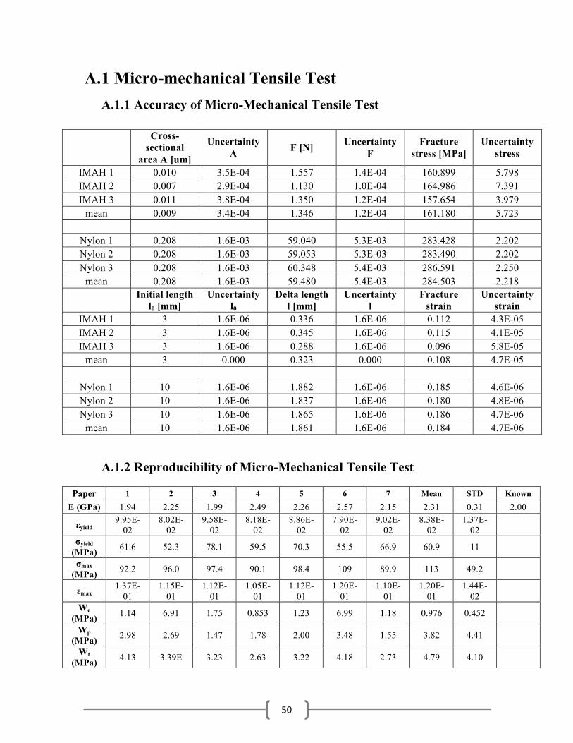
50

A. 1 Micro-mechanical Tensile Test A.1.1 Accuracy of Micro-Mechanical Tensile Test

Cross-

sectional area A [um]

Uncertainty A F [N] Uncertainty

F Fracture

stress [MPa] Uncertainty

stress

IMAH 1 0.010 3.5E-04 1.557 1.4E-04 160.899 5.798 IMAH 2 0.007 2.9E-04 1.130 1.0E-04 164.986 7.391 IMAH 3 0.011 3.8E-04 1.350 1.2E-04 157.654 3.979

mean 0.009 3.4E-04 1.346 1.2E-04 161.180 5.723

Nylon 1 0.208 1.6E-03 59.040 5.3E-03 283.428 2.202 Nylon 2 0.208 1.6E-03 59.053 5.3E-03 283.490 2.202 Nylon 3 0.208 1.6E-03 60.348 5.4E-03 286.591 2.250

mean 0.208 1.6E-03 59.480 5.4E-03 284.503 2.218

Initial length l0 [mm]

Uncertainty l0

Delta length l [mm]

Uncertainty l

Fracture strain

Uncertainty strain

IMAH 1 3 1.6E-06 0.336 1.6E-06 0.112 4.3E-05 IMAH 2 3 1.6E-06 0.345 1.6E-06 0.115 4.1E-05 IMAH 3 3 1.6E-06 0.288 1.6E-06 0.096 5.8E-05

mean 3 0.000 0.323 0.000 0.108 4.7E-05

Nylon 1 10 1.6E-06 1.882 1.6E-06 0.185 4.6E-06 Nylon 2 10 1.6E-06 1.837 1.6E-06 0.180 4.8E-06 Nylon 3 10 1.6E-06 1.865 1.6E-06 0.186 4.7E-06

mean 10 1.6E-06 1.861 1.6E-06 0.184 4.7E-06

A.1.2 Reproducibility of Micro-Mechanical Tensile Test

Paper 1 2 3 4 5 6 7 Mean STD Known E (GPa) 1.94 2.25 1.99 2.49 2.26 2.57 2.15 2.31 0.31 2.00

εyield 9.95E-02

8.02E-02

9.58E-02

8.18E-02

8.86E-02

7.90E-02

9.02E-02

8.38E-02

1.37E-02

σyield (MPa) 61.6 52.3 78.1 59.5 70.3 55.5 66.9 60.9 11 σmax

(MPa) 92.2 96.0 97.4 90.1 98.4 109 89.9 113 49.2

εmax 1.37E-

01 1.15E-

01 1.12E-

01 1.05E-

01 1.12E-

01 1.20E-

01 1.10E-

01 1.20E-

01 1.44E-

02 We

(MPa) 1.14 6.91 1.75 0.853 1.23 6.99 1.18 0.976 0.452 Wp

(MPa) 2.98 2.69 1.47 1.78 2.00 3.48 1.55 3.82 4.41 Wt

(MPa) 4.13 3.39E 3.23 2.63 3.22 4.18 2.73 4.79 4.10

51

A.1.2.1 Mechanical Parameters Immature Bone

A.1.2.2 Mechanical Parameters of Mature bone

1 2 3 4 5 6 7 8 9 10 11 12 Mean STD

E (GPa)

2.47 4.23 1.73 1.04 3.85 2.84 3.60 1.57 1.64 7.64 5.43 3.38 3.29 1.88

εyield 2.71E-02

4.01E-02

4.24E-02

4.54E-02

1.96E-02

2.95E-02

3.51E-02

4.44E-02

2.17E-02

1.90E-02

2.50E-02

2.14E-02

3.09E-02

1.01E-02

σyield (MPa)

63.3 92.2 39.4 54.0 55.8 57.4 79.5 27.3 25.8 88.7 92.8 61.3 61.5 23.4

σmax (MPa)

72.2 141 44.5 72.7 115 89.9 103 119 63.9 178 163 125 107 40.8

εmax 3.68E-02

9.58E-02

5.00E-02

1.11E-01

7.51E-02

5.10E-02

5.49E-02

7.40E-02

1.01E-01

8.83E-02

9.52E-02

9.67E-02

7.75E-02

2.43E-02

We (MPa)

0.902

1.25 0.546

1.36 0.508

0.685

0.108

0.360

0.252

0.688

0.998

0.648

0.774

0.348

Wp (MPa)

0.67 6.37 0.32 4.30 4.20 1.33 1.77 1.45 3.66 9.51 9.25 6.73 4.13 3.22

Wt (MPa)

1.57 7.62 8.67 5.66 4.71 2.02 2.85 1.81 3.91 10.2 10.2 7.38 4.90 3.32

1 2 3 4 5 6 7 8 9 Mean STD E (GPa) 5.48 6.21 4.32 6.78 2.66 4.89 7.50 4.81 4.72 5.26 1.44

εyield 2.29E-02

2.53E-02

1.45E-02

1.71E-02

3.47E-02

2.91E-02

9.76E-03

3.20E-02

2.24E-02

2.31E-02

8.23E-03

σyield (MPa) 84.8 101 43.0 76.9 73.1 86.1 51.2 73.9 64.8 72.8 17.9

σmax (MPa) 201 105 176 152 122 984 145 201 154 150 377

εmax 3.51E-

02 2.68E-

02 9.79E-

02 8.72E-

02 1.77E-

01 3.99E-

02 6.28E-

02 5.19E-

02 3.21E-

02 6.79E-

02 4.79E-

02 We

(MPa) 0.855 1.05 0.309 0.587 1.14 0.971 0.273 0.769 0.59 0.727 0.310

Wp (MPa) 1.07 1.54 7.69 7.56 14.6 0.864 3.72 1.79 0.61 4.23 4.85

Wt (MPa) 1.93 1.20 8.00 8.15 1.58 1.83 3.99 2.56 1.20 4.96 4.88

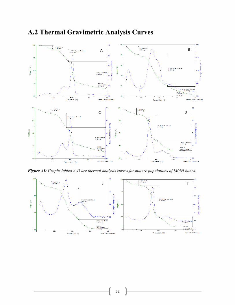
52

A.2 Thermal Gravimetric Analysis Curves

Figure AI: Graphs labled A-D are thermal analysis curves for mature populations of IMAH bones.

A B

C

E

D

F

53

Figure A2: Graphs labled E-G are thermal analysis curves for immature populations. Parameters determined from these curves are depicted in Tables 3-3 and 3-4.

G

54

A.3 Matlab Scripts A.3.1 Macro-scale Assessment

A.3.1.1 Cross-sectional Area determined from pixel images from µCT.

% This script has been dedicated to microCT images of Herring fishbone samples / microsamples % It evaluates the following properties of a stack of images acquired from % one individual bone sample: % - bone mineral densitymeanBMD per slice % - standard deviation SDBMD for mean BMD per slice % - crossectional area per slice % - plot of BMD=-SD over slice number % - plot of crossectional area pver slice number clc; clear all; close all; % load bmp images [fileName, path]=uigetfile('*.bmp', 'Select one image in the stack you need to analyse', '/home/berteaulab3/IMKE/H4_R/REC'); pics = dir([path, '*.bmp']); % defining output vectors for BMD, SD and Area % zeros creates array of all zeros SDBMD = zeros(size(pics,1),1); BMDmean = zeros(size(pics,1),1); CSarea = zeros(size(pics,1),1); bonebegin=zeros(size(pics,1),1); boneend=zeros(size(pics,1),1); % loop from the first line to the last line of the pics structures (scan through all images one by one) for i=1:size(pics,1) % i is the number of images / slices within pics image=imread(strcat(path, pics(i).name)); % read image, whereby origin of image is concatinated mask=image>100; % threshhold at gv=100 CSarea(i)=sum(sum(mask==1))*25.025*10^-6; % counting the number of pixels in the mask and

multiply by pixel area end figure(1); subplot(3,1,2); plot(CSarea); axis([ 0 3000 0 0.03]) ylabel('Cross-sectional area in mm^2'); xlabel('slice number'); hold on; filename='RESULTS.csv'; results=[CSarea]; xlswrite(filename,results); A.3.1.2 Micro-Mechanical Tensile Properties

clear all; close all; clc; [fileName, path] = uigetfile({'*'}, 'Select the folder', '../'); fileNameArray = strsplit(fileName, '.');%Extracting the extension of the chosen file extension = fileNameArray(end); fileNameType = strcat(path, '*.', extension); files = dir(fileNameType{1,1}); number= size(files, 1); num = xlsread(strcat(path,'Infos.xlsx')); area1=num(:,7); % Diameter2=num(:,6); Distance=num(:,8); res={ 'FISH',' ' ;... 'MOE',0 ;... 'Yield strain',0;... 'Yield stress',0;... 'Maximum stress',0; ... 'Maximum strain',0;... 'Elastic work',0;... 'Plastic work',0;... 'Total work',0}; %xlswrite(stract(path,'res',res)); %% Initialize variables. startRow = 2;

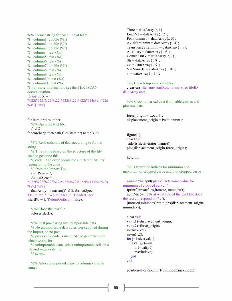
55

%% Format string for each line of text: % column1: double (%f) % column2: double (%f) % column3: double (%f) % column4: text (%s) % column5: text (%s) % column6: text (%s) % column7: double (%f) % column8: text (%s) % column9: text (%s) % column10: text (%s) % column11: text (%s) % For more information, see the TEXTSCAN documentation. formatSpec = '%22f%22f%22f%22s%22s%22s%22f%13s%4s%2s%s%[^\n\r]'; for iterator=1:number %% Open the text file. fileID = fopen(char(strcat(path,files(iterator).name)),'r'); %% Read columns of data according to format string. % This call is based on the structure of the file used to generate this % code. If an error occurs for a different file, try regenerating the code % from the Import Tool. startRow = 2; formatSpec = '%22f%22f%22f%22s%22s%22s%22f%13s%4s%2s%s%[^\n\r]'; dataArray = textscan(fileID, formatSpec, 'Delimiter', '', 'WhiteSpace', '', 'HeaderLines' ,startRow-1, 'ReturnOnError', false); %% Close the text file. fclose(fileID); %% Post processing for unimportable data. % No unimportable data rules were applied during the import, so no post % processing code is included. To generate code which works for % unimportable data, select unimportable cells in a file and regenerate the % script. %% Allocate imported array to column variable names

Time = dataArray{:, 1}; LoadN1 = dataArray{:, 2}; Positionmm1 = dataArray{:, 3}; AxialStrainmm = dataArray{:, 4}; TransverseStrainmm = dataArray{:, 5}; Auxiliary = dataArray{:, 6}; ControlOutV = dataArray{:, 7}; Str = dataArray{:, 8}; ess = dataArray{:, 9}; VarName10 = dataArray{:, 10}; si = dataArray{:, 11}; %% Clear temporary variables clearvars filename startRow formatSpec fileID dataArray ans; %% Crop numerical data from table entries and plot raw data force_origin = LoadN1; displacement_origin = Positionmm1; figure(1); clear title title(((files(iterator).name))); plot(displacement_origin,force_origin); hold on; %% Determine indices for minimum and maximum of cropped curve and plot cropped curve minindex=input('please Determine value for minimum of cropped curve: '); fprintf(strcat(files(iterator).name,'\n')); numMice=input('at what line of the exel file does the test correspond on ? : '); [notused,minindex]=min(abs(displacement_origin-minindex)); clear val; val(:,1)=displacement_origin; val(:,2)=force_origin; m=max(val); m=m(1,2); for j=1:size(val,1) if val(j,2)==m m1=val(j,1); maxindex=j; end end position=Positionmm1(minindex:maxindex);

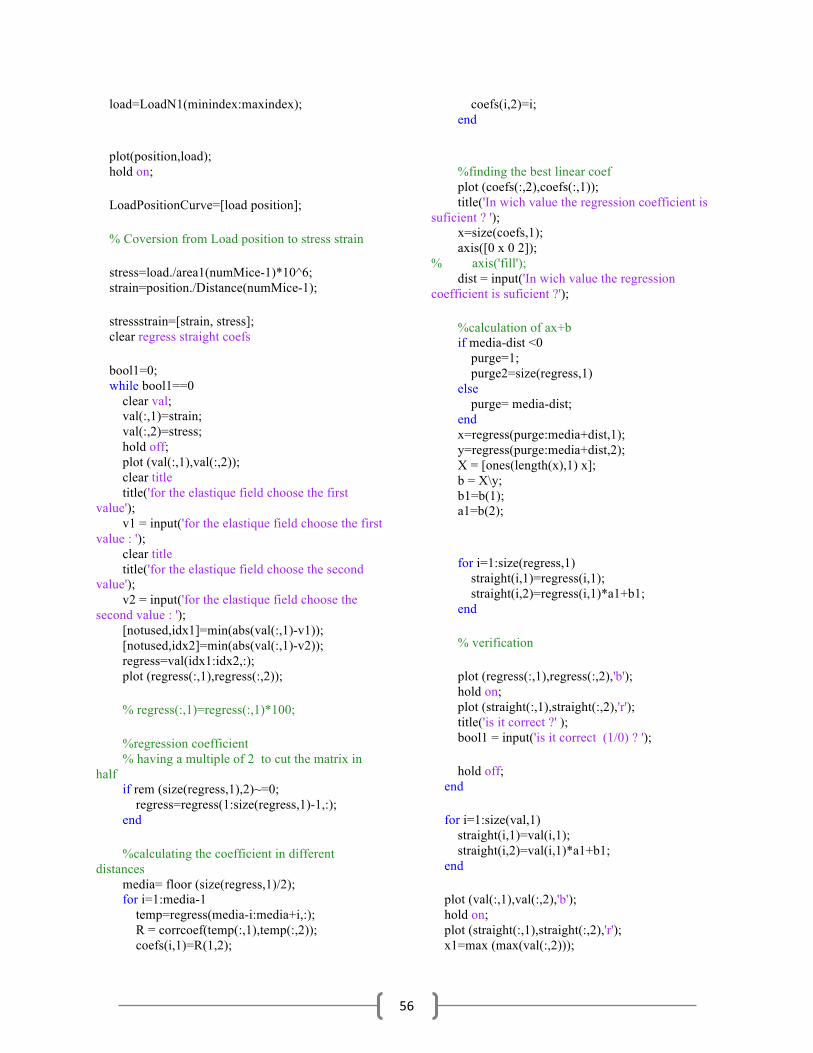
56

load=LoadN1(minindex:maxindex); plot(position,load); hold on; LoadPositionCurve=[load position]; % Coversion from Load position to stress strain stress=load./area1(numMice-1)*10^6; strain=position./Distance(numMice-1); stressstrain=[strain, stress]; clear regress straight coefs bool1=0; while bool1==0 clear val; val(:,1)=strain; val(:,2)=stress; hold off; plot (val(:,1),val(:,2)); clear title title('for the elastique field choose the first value'); v1 = input('for the elastique field choose the first value : '); clear title title('for the elastique field choose the second value'); v2 = input('for the elastique field choose the second value : '); [notused,idx1]=min(abs(val(:,1)-v1)); [notused,idx2]=min(abs(val(:,1)-v2)); regress=val(idx1:idx2,:); plot (regress(:,1),regress(:,2)); % regress(:,1)=regress(:,1)*100; %regression coefficient % having a multiple of 2 to cut the matrix in half if rem (size(regress,1),2)~=0; regress=regress(1:size(regress,1)-1,:); end %calculating the coefficient in different distances media= floor (size(regress,1)/2); for i=1:media-1 temp=regress(media-i:media+i,:); R = corrcoef(temp(:,1),temp(:,2)); coefs(i,1)=R(1,2);

coefs(i,2)=i; end %finding the best linear coef plot (coefs(:,2),coefs(:,1)); title('In wich value the regression coefficient is suficient ? '); x=size(coefs,1); axis([0 x 0 2]); % axis('fill'); dist = input('In wich value the regression coefficient is suficient ?'); %calculation of ax+b if media-dist <0 purge=1; purge2=size(regress,1) else purge= media-dist; end x=regress(purge:media+dist,1); y=regress(purge:media+dist,2); X = [ones(length(x),1) x]; b = X\y; b1=b(1); a1=b(2); for i=1:size(regress,1) straight(i,1)=regress(i,1); straight(i,2)=regress(i,1)*a1+b1; end % verification plot (regress(:,1),regress(:,2),'b'); hold on; plot (straight(:,1),straight(:,2),'r'); title('is it correct ?' ); bool1 = input('is it correct (1/0) ? '); hold off; end for i=1:size(val,1) straight(i,1)=val(i,1); straight(i,2)=val(i,1)*a1+b1; end plot (val(:,1),val(:,2),'b'); hold on; plot (straight(:,1),straight(:,2),'r'); x1=max (max(val(:,2)));

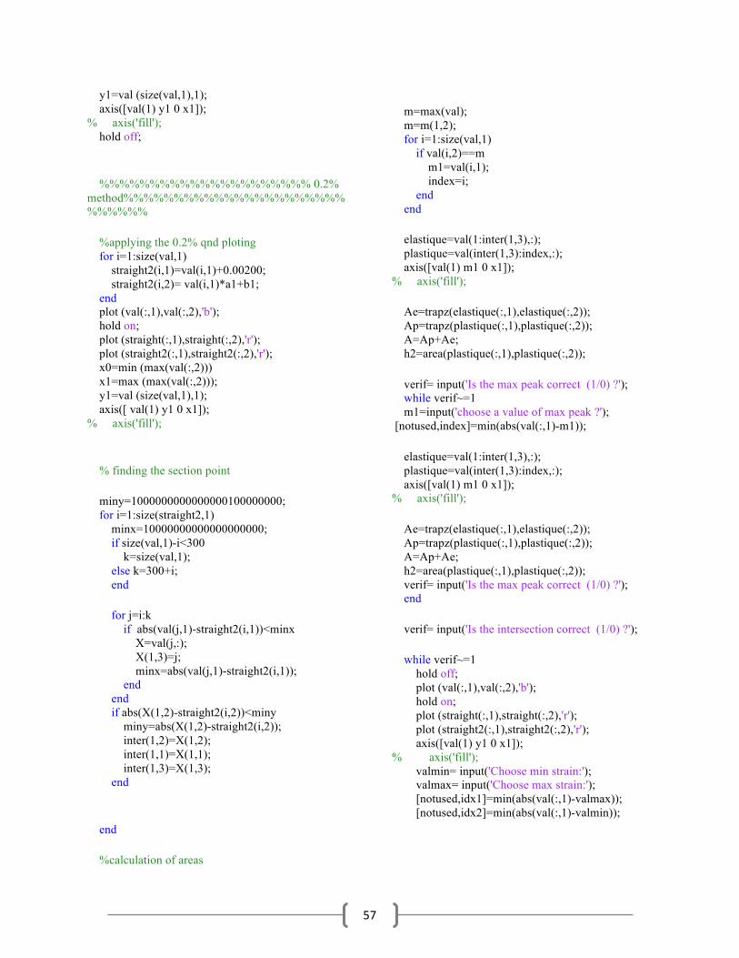
57

y1=val (size(val,1),1); axis([val(1) y1 0 x1]); % axis('fill'); hold off; %%%%%%%%%%%%%%%%%%%%% 0.2% method%%%%%%%%%%%%%%%%%%%%%%%%%%%% %applying the 0.2% qnd ploting for i=1:size(val,1) straight2(i,1)=val(i,1)+0.00200; straight2(i,2)= val(i,1)*a1+b1; end plot (val(:,1),val(:,2),'b'); hold on; plot (straight(:,1),straight(:,2),'r'); plot (straight2(:,1),straight2(:,2),'r'); x0=min (max(val(:,2))) x1=max (max(val(:,2))); y1=val (size(val,1),1); axis([ val(1) y1 0 x1]); % axis('fill'); % finding the section point miny=1000000000000000100000000; for i=1:size(straight2,1) minx=10000000000000000000; if size(val,1)-i<300 k=size(val,1); else k=300+i; end for j=i:k if abs(val(j,1)-straight2(i,1))<minx X=val(j,:); X(1,3)=j; minx=abs(val(j,1)-straight2(i,1)); end end if abs(X(1,2)-straight2(i,2))<miny miny=abs(X(1,2)-straight2(i,2)); inter(1,2)=X(1,2); inter(1,1)=X(1,1); inter(1,3)=X(1,3); end end %calculation of areas

m=max(val); m=m(1,2); for i=1:size(val,1) if val(i,2)==m m1=val(i,1); index=i; end end elastique=val(1:inter(1,3),:); plastique=val(inter(1,3):index,:); axis([val(1) m1 0 x1]); % axis('fill'); Ae=trapz(elastique(:,1),elastique(:,2)); Ap=trapz(plastique(:,1),plastique(:,2)); A=Ap+Ae; h2=area(plastique(:,1),plastique(:,2)); verif= input('Is the max peak correct (1/0) ?'); while verif~=1 m1=input('choose a value of max peak ?'); [notused,index]=min(abs(val(:,1)-m1)); elastique=val(1:inter(1,3),:); plastique=val(inter(1,3):index,:); axis([val(1) m1 0 x1]); % axis('fill'); Ae=trapz(elastique(:,1),elastique(:,2)); Ap=trapz(plastique(:,1),plastique(:,2)); A=Ap+Ae; h2=area(plastique(:,1),plastique(:,2)); verif= input('Is the max peak correct (1/0) ?'); end verif= input('Is the intersection correct (1/0) ?'); while verif~=1 hold off; plot (val(:,1),val(:,2),'b'); hold on; plot (straight(:,1),straight(:,2),'r'); plot (straight2(:,1),straight2(:,2),'r'); axis([val(1) y1 0 x1]); % axis('fill'); valmin= input('Choose min strain:'); valmax= input('Choose max strain:'); [notused,idx1]=min(abs(val(:,1)-valmax)); [notused,idx2]=min(abs(val(:,1)-valmin));

58

% finding the section point miny=100000000000000000000000000; for i=idx2:size(straight2,1) minx=1000000000000000000000000; if idx1-i<300 k=idx1; else k=300+i; end for j=i:k if abs(val(j,1)-straight2(i,1))<minx X=val(j,:); X(1,3)=j; minx=abs(val(j,1)-straight2(i,1)); end end if abs(X(1,2)-straight2(i,2))<miny miny=abs(X(1,2)-straight2(i,2)); inter(1,2)=X(1,2); inter(1,1)=X(1,1); inter(1,3)=X(1,3); end end %calculation of areas elastique=val(1:inter(1,3),:); plastique=val(inter(1,3):index,:); axis([x0 m1 0 x1]); % axis('fill'); Ae=trapz(elastique(:,1),elastique(:,2)); Ap=trapz(plastique(:,1),plastique(:,2)); A=Ap+Ae; h2=area(plastique(:,1),plastique(:,2)); verif= input('Is it correct (1/0) ?'); xlabel('Srain') ylabel('Stress') end res(1,iterator+1)={files(iterator).name}; res(2,iterator+1)={a1}; res(3,iterator+1)={inter(1,1)}; res(4,iterator+1)={inter(1,2)}; res(5,iterator+1)={m};

res(6,iterator+1)={m1}; res(7,iterator+1)={Ae}; res(8,iterator+1)={Ap}; res(9,iterator+1)={A}; fprintf('MOE: %f \n',a1); fprintf('Yield strain: %f\n',inter(1,1)); fprintf('Yield strain stress: %f\n',inter(1,2)); fprintf('Maximum stress : %f\n',m); fprintf('Maximum stress strain: %f\n',m1); fprintf('Elastic work: %f\n',Ae); fprintf('Plastic work: %f\n',Ap); fprintf('Total work: %f\n',A); ylabel('Stress in Pa'); xlabel('Strain'); % mTextBox = uicontrol('style','text'); % set(mTextBox,'String','Elastic Region'); % set(mTextBox,'String','Plastic Region'); print((strcat(path,files(iterator).name,'.png')),'-dpng'); xlswrite(strcat(path,'/res'),res) hold off end xlswrite(strcat(path,'/res'),res)

59

A.3.2 Matlab: Crystallinity ratio and Crystallinity Index

Three functions and one .m script were used

simultaneously.

A.3.2.1 Peak Analysis function: Isolates peaks of interest

function [results,FitResults] = peakanalyziselevenLana(K,L,Data,a) % cut to have just the peak idx= a>=K & a<=L; %interval of Raman Shift for Phosphate peak index=find(idx); % Matrix index (place of Phosphate peak on Data) PeakVfourPhosphate=Data(index',:); %extraxtion of the matrix of Phosphate peak x=PeakVfourPhosphate(:,1); y=PeakVfourPhosphate(:,2); % to draw the curve % Find a spline to approximate the peak newY=spline4(x,y); y=newY; % PeakPhosphate(:,2)=y % Maximum of the peak and middle of maximum max0=max(y) ; % maximum of the peak MiddlePeak=max0/2; % middle of the maximum of peak %Find the raman shifts corresponding to the middle of maximum of peak indexmax=find(y==max0); % find the index for the max PeakPhosphate1=PeakVfourPhosphate(1:indexmax,:) ; %create two matrices : one before the max, one after the max PeakPhosphate2=PeakVfourPhosphate(indexmax+1:length(PeakVfourPhosphate),:); [i1,j1]=find(PeakPhosphate1(:,2)>MiddlePeak); %find the coordinate of the numbers biggest than MiddlePeak i1=i1(1); %take the to MiddlePeak X1=PeakPhosphate1(i1,1); %find its Raman shift corresponding [i2,j2]=find(PeakPhosphate2>MiddlePeak); % same

thing if isempty(i2) ; % if there is no value closer to MiddlePeak (if it is like a half peak) X2=0 ; % put 0 for the secund Raman shift end if ~isempty(i2); % if there is one i2=i2(end); % take the last value X2=PeakPhosphate2(i2,1); % find the Raman shift corresponding end if X2==0; width=0; %find the width of the Phosphate peak for the point : Middle peak end if X2~=0; width=X2-X1; %width of the peak in the half of max end % calculate the area under the curve area=trapz(x,y); % find th area under the curve of Phosphate Peak % matrix of all results results=[max0,MiddlePeak,X1,X2,width,area]; % Data processing for v3 phosphate if K==900 % x=X; % y=Y; %Parameters for peakfit x=fix(x); y=y'; AmideI=[x y]; indexAmideIb=find(AmideI(:,1)==900); if isempty(indexAmideIb); [i6,j6]=find(AmideI(:,1)>900) ;

60

i6=i6(1); %take the closer to MiddlePeak AmideI=AmideI(i6:length(AmideI),:); else AmideI=AmideI(indexAmideIb:length(AmideI),:) ; end indexAmideIe=find(AmideI(:,1)==1200) ; if isempty(indexAmideIe); [i7,j7]=find(AmideI(:,1)>1200); i7=i7(1); AmideI=AmideI(1:i7,:); else AmideI=AmideI(1:indexAmideIe,:); end signal=AmideI; window=max(AmideI(:,1))-min(AmideI(:,1)); center=max(AmideI(:,1))-window/2; NumPeaks=2; peakshape=16; %%fixed position Gauss NumTrials=20; start=[center window]; autozero=1; %AUTOZERO=0 plots=1; %subPeakAmideI=[1606 1627 1642 1665 1684 1690];%work work %subPeakAmideI=[1605 1636 1662 1687] % 1606 1641 1667 1689 %subpeak for mice 1606 1643 1665 1686 subPeakAmideI=[1020 1030] %subPeakAmideI=[1635 1666 1690] for i=1:length(subPeakAmideI); fixedparameters(i)=subPeakAmideI(i); end; extra=0; bipolar=0; minwidth=10; DELTA=1.0; clipheight=20000; [FitResults]=peakfit(signal,center,window,NumPeaks,peakshape,extra,NumTrials,start,autozero,fixedparameters,plots,bipolar,minwidth,DELTA,clipheight); else FitResults=0; end end

A.3.2.2 Peak fit: Curve fitting

function [FitResults,GOF,baseline,coeff,residual,xi,yi,BootResults]=peakfit(signal,center,window,NumPeaks,peakshape,extra,NumTrials,start,autozero,fixedparameters,plots,bipolar,minwidth,DELTA,clipheight) % A command-line peak fitting program for time-series signals, written as a % self-contained Matlab function in a single m-file. Uses a non-linear % optimization algorithm to decompose a complex, overlapping-peak signal % into its component parts. The objective is to determine whether your % signal can be represented as the sum of fundamental underlying peaks % shapes. Accepts signals of any length, including those with non-integer % and non-uniform x-values. Fits any number of peaks of any of 33 curve % shapes. This is a command line version, usable from a remote terminal. It % is capable of making multiple trial fits with sightly different starting % values (whose variability is controled by the 14th input argument) and % taking the one with the lowest mean fit error (example 6). It can % estimate the standard deviation of peak parameters from a single signal % using the bootstrap method (example 10). % % Version 7.45: September, 2015, Reports FWHM for Voigt shapes (shape % numbers 20 and 30). % % For more details, see % http://terpconnect.umd.edu/~toh/spectrum/CurveFittingC.html and % http://terpconnect.umd.edu/~toh/spectrum/InteractivePeakFitter.htm % % peakfit(signal); % Performs an iterative least-squares fit of a single Gaussian peak to the % data matrix "signal", which has x values in column 1 and Y values in % column 2 (e.g. [x y]) % % peakfit(signal,center,window); % Fits a single Gaussian peak to a portion of the matrix "signal". The

61

% portion is centered on the x-value "center" and has width "window" (in x % units). % % peakfit(signal,center,window,NumPeaks); % "NumPeaks" = number of peaks in the model (default is 1 if not % specified). No limit to maximum number of peaks in version 3.1 % % peakfit(signal,center,window,NumPeaks,peakshape); % "peakshape" specifies the peak shape of the model: (1=Gaussian (default), % 2=Lorentzian, 3=logistic distribution, 4=Pearson, 5=exponentionally % broadened Gaussian; 6=equal-width Gaussians; 7=Equal-width Lorentzians; % 8=exponentionally broadened equal-width Gaussian, 9=exponential pulse, % 10=up-sigmoid (logistic function), 11=Fixed-width Gaussian, % 12=Fixed-width Lorentzian; 13=Gaussian/ Lorentzian blend; 14=Bifurcated % Gaussian, 15=Breit-Wigner-Fano, 16=Fixed-position Gaussians; % 17=Fixed-position Lorentzians; 18=exponentionally broadened Lorentzian; % 19=alpha function; 20=Voigt profile; 21=triangular; 22=multiple shapes; % 23=down-sigmoid; 25=lognormal; 26=slope; 27=Gaussian first derivative; % 28=polynomial; 29=piecewise linear; 30=variable-alpha Voigt; 31=variable % time constant ExpGaussian; 32=variable Pearson; 33=variable % Gaussian/Lorentzian blend % % peakfit(signal,center,window,NumPeaks,peakshape,extra) % 'extra' specifies the value of 'extra', used only in the Voigt, Pearson, % exponentionally broadened Gaussian, Gaussian/Lorentzian blend, and % bifurcated Gaussian and Lorentzian shapes to fine-tune the peak shape. % % peakfit(signal,center,window,NumPeaks,peakshape,extra,NumTrials); % Performs "NumTrials" trial fits and selects the best one (with lowest % fitting error). NumTrials can be any positive integer (default is 1). %

% peakfit(signal,center,window,NumPeaks,peakshape,extra,NumTrials,start) % Specifies the first guesses vector "firstguess" for the peak positions % and widths. Must be expressed as a vector , in square brackets, e.g. % start=[position1 width1 position2 width2 ...] % % peakfit(signal,center,window,NumPeaks,peakshape,extra,NumTrials,start,autozero) % 'autozero' sets the baseline correction mode: % autozero=0 (default) does not subtract baseline from data segment; % autozero=1 interpolates a linear baseline from the edges of the data % segment and subtracts it from the signal (assumes that the % peak returns to the baseline at the edges of the signal); % autozero=2 is like mode 1 except that it computes a quadratic curved baseline; % autozero=3 compensates for a flat baseline without reference to the % signal itself (best if the peak does not return to the % baseline at the edges of the signal). % % peakfit(signal,center,window,NumPeaks,peakshape,extra,NumTrials,start,... % autozero,fixedparameters) % 'fixedparameters' specifies fixed values for widths (shapes 10, 11) or % positions (shapes 16, 17) % % peakfit(signal,center,window,NumPeaks,peakshape,extra,NumTrials,start,... % autozero,fixedparameters,plots) % 'plots' controls graphic plotting: 0=no plot; 1=plots draw as usual (default) % % peakfit(signal,center,window,NumPeaks,peakshape,extra,NumTrials,start,... % autozero,fixedparameters,plots,bipolar) % 'bipolar' = 0 constrain peaks heights to be positions; 'bipolar' = 1 % allows positive ands negative peak heights. % % peakfit(signal,center,window,NumPeaks,peakshape,extra,NumTrials,start,... % autozero,fixedparameters,plots,bipolar,minwidth)

62

% 'minwidth' sets the minmimum allowed peak width. The default if not % specified is equal to the x-axis interval. Must be a vector of minimum % widths, one value for each peak, if the multiple peak shape is chosen, % as in example 17 and 18. % % peakfit(signal,center,window,NumPeaks,peakshape,extra,NumTrials,start,... % autozero,fixedparameters,plots,bipolar,minwidth) % 'DELTA' (14th input argument) controls the restart variance when % NumTrials>1. Default value is 1.0. Larger values give more variance. % Version 5.8 and later only. % [FitResults,FitError]=peakfit(signal,center,window...) Returns the % FitResults vector in the order peak number, peak position, peak height, % peak width, and peak area), and the FitError (the percent RMS % difference between the data and the model in the selected segment of that % data) of the best fit. % % [FitResults,LowestError,BestStart,xi,yi,BootResults]=peakfit(signal,...) % Prints out parameter error estimates for each peak (bootstrap method). % % Optional output parameters % 1. FitResults: a table of model peak parameters, one row for each peak, % listing Peak number, Peak position, Height, Width, and Peak area. % 2. GOF: Goodness of Fit, a vector containing the rms fitting error of the % best trial fit and the R-squared (coefficient of determination). % 3. Baseline, the polynomial coefficients of the baseline in linear % and quadratic baseline modes (1 and 2) or the value of the constant % baseline in flat baseline mode. % 3. coeff: Coefficients for the polynomial fit (shape 28 only; for other % shapes, coeff=0) % 5. residual: the difference between the data and the best fit. % 6. xi: vector containing 600 interploated x-values for the model peaks. % 7. yi: matrix containing the y values of each model

peak at each xi. % Type plot(xi,yi(1,:)) to plot peak 1 or plot(xi,yi) to plot all peaks % 8. BootResults: a table of bootstrap precision results for a each peak % and peak parameter. % % Example 1: % >> x=[0:.1:10]';y=exp(-(x-5).^2);peakfit([x y]) % Fits exp(-x)^2 with a single Gaussian peak model. % % Peak number Peak position Height Width Peak area % 1 5 1 1.665 1.7725 % % >> y=[0 1 2 4 6 7 6 4 2 1 0 ];x=1:length(y); % >> peakfit([x;y],length(y)/2,length(y),0,0,0,0,0,0) % Fits small set of manually entered y data to a single Gaussian peak model. % % Example 2: % x=[0:.01:10];y=exp(-(x-5).^2)+randn(size(x));peakfit([x;y]) % Measurement of very noisy peak with signal-to-noise ratio = 1. % ans = % 1 5.0279 0.9272 1.7948 1.7716 % % Example 3: % x=[0:.1:10];y=exp(-(x-5).^2)+.5*exp(-(x-3).^2)+.1*randn(size(x)); % peakfit([x' y'],0,0,2) % Fits a noisy two-peak signal with a double Gaussian model (NumPeaks=2). % ans = % 1 3.0001 0.49489 1.642 0.86504 % 2 4.9927 1.0016 1.6597 1.7696 % % Example 4: % >> x=1:100;y=ones(size(x))./(1+(x-50).^2);peakfit(y,0,0,1,2) % Fit Lorentzian (peakshape=2) located at x=50, height=1, width=2. % ans = % 1 50 0.99974 1.9971 3.1079 % % Example 5: % >> x=[0:.005:1];y=humps(x);peakfit([x' y'],.3,.7,1,4,3); % Fits a portion of the humps function, 0.7 units wide and centered on % x=0.3, with a single (NumPeaks=1) Pearson

63

function (peakshape=4) with % extra=3 (controls shape of Pearson function). % % Example 6: % >> x=[0:.005:1];y=(humps(x)+humps(x-.13)).^3;smatrix=[x' y']; % >> [FitResults,FitError]=peakfit(smatrix,.4,.7,2,1,0,10) % Creates a data matrix 'smatrix', fits a portion to a two-peak Gaussian % model, takes the best of 10 trials. Returns FitResults and FitError. % FitResults = % 1 0.31056 2.0125e+006 0.11057 2.3689e+005 % 2 0.41529 2.2403e+006 0.12033 2.8696e+005 % FitError = % 1.1899 % % Example 7: % >> peakfit([x' y'],.4,.7,2,1,0,10,[.3 .1 .5 .1]); % As above, but specifies the first-guess position and width of the two % peaks, in the order [position1 width1 position2 width2] % % Example 8: (Version 4 only) % Demonstration of the four autozero modes, for a single Gaussian on flat % baseline, with position=10, height=1, and width=1.66. Autozero mode % is specified by the 9th input argument (0,1,2, or 3). % >> x=8:.05:12;y=1+exp(-(x-10).^2); % >> [FitResults,FitError]=peakfit([x;y],0,0,1,1,0,1,0,0) % Autozero=0 means to ignore the baseline (default mode if not specified) % FitResults = % 1 10 1.8561 3.612 5.7641 % FitError = % 5.387 % >> [FitResults,FitError]=peakfit([x;y],0,0,1,1,0,1,0,1) % Autozero=1 subtracts linear baseline from edge to edge. % Does not work well because signal does not return to baseline at edges. % FitResults = % 1 9.9984 0.96153 1.559 1.5916 % FitError = % 1.9801 % >> [FitResults,FitError]=peakfit([x;y],0,0,1,1,0,1,0,2)

% Autozero=1 subtracts quadratic baseline from edge to edge. % Does not work well because signal does not return to baseline at edges. % FitResults = % 1 9.9996 0.81749 1.4384 1.2503 % FitError = % 1.8204 % Autozero=3: Flat baseline mode, measures baseline by regression % >> [FitResults,Baseline,FitError]=peakfit([x;y],0,0,1,1,0,1,0,3) % FitResults = % 1 10 1.0001 1.6653 1.7645 % Baseline = % 0.0037056 % FitError = % 0.99985 % % Example 9: % x=[0:.1:10];y=exp(-(x-5).^2)+.5*exp(-(x-3).^2)+.1*randn(size(x)); % [FitResults,FitError]=peakfit([x' y'],0,0,2,11,0,0,0,0,1.666) % Same as example 3, fit with fixed-width Gaussian (shape 11), width=1.666 % % Example 10: (Version 3 or later; Prints out parameter error estimates) % x=0:.05:9;y=exp(-(x-5).^2)+.5*exp(-(x-3).^2)+.01*randn(1,length(x)); % [FitResults,LowestError,residuals,xi,yi,BootstrapErrors]=peakfit([x;y],0,0,2,6,0,1,0,0,0); % % Example 11: (Version 3.2 or later) % x=[0:.005:1];y=humps(x);[FitResults,FitError]=peakfit([x' y'],0.54,0.93,2,13,15,10,0,0,0) % % FitResults = % 1 0.30078 190.41 0.19131 23.064 % 2 0.89788 39.552 0.33448 6.1999 % FitError = % 0.34502 % Fits both peaks of the Humps function with a Gaussian/Lorentzian blend % (shape 13) that is 15% Gaussian (Extra=15). % % Example 12: (Version 3.2 or later) % >> x=[0:.1:10];y=exp(-(x-4).^2)+.5*exp(-(x-

64

5).^2)+.01*randn(size(x)); % >> [FitResults,FitError]=peakfit([x' y'],0,0,1,14,45,10,0,0,0) % FitResults = % 1 4.2028 1.2315 4.077 2.6723 % FitError = % 0.84461 % Fit a slightly asymmetrical peak with a bifurcated Gaussian (shape 14) % % Example 13: (Version 3.3 or later) % >> x=[0:.1:10]';y=exp(-(x-5).^2);peakfit([x y],0,0,1,1,0,0,0,0,0,0) % Example 1 without plotting (11th input argument = 0, default is 1) % % Example 14: (Version 3.9 or later) % Exponentially broadened Lorentzian with position=9, height=1. % x=[0:.1:20]; % L=lorentzian(x,9,1); % L1=ExpBroaden(L',-10)+0.02.*randn(size(x))'; % [FitResults,FitError]=peakfit([x;L1'],0,0,1,18,10) % % Example 15: Fitting humps function with two Voigts (version 7.45) % FitResults,FitError]=peakfit(humps(0:.01:2),60,120,2,20,1.7,5,0) % FitResults = % 1 31.099 94.768 19.432 2375.3 % 2 90.128 20.052 32.973 783.34 % FitError = % 0.72829 0.99915 % % Example 16: (Version 4.3 or later) Set +/- mode to 1 (bipolar) % >> x=[0:.1:10];y=exp(-(x-5).^2)-.5*exp(-(x-3).^2)+.1*randn(size(x)); % >> peakfit([x' y'],0,0,2,1,0,1,0,0,0,1,1) % FitResults = % 1 3.1636 -0.5433 1.62 -0.9369 % 2 4.9487 0.96859 1.8456 1.9029 % FitError = % 8.2757 % % Example 17: Version 5 or later. Fits humps function to a model consisting % of one Pearson (shape=4, extra=3) and one Gaussian (shape=1), flat % baseline mode=3, NumTrials=10.

% x=[0:.005:1.2];y=humps(x);[FitResults,FitError]=peakfit([x' y'],0,0,2,[2 1],[0 0]) % FitResults = % 1 0.30154 84.671 0.27892 17.085 % 2 0.88522 11.545 0.20825 2.5399 % Baseline = % 0.901 % FitError = % 10.457 % % Example 18: 5 peaks, 5 different shapes, all heights = 1, widths = 3. % x=0:.1:60; % y=modelpeaks2(x,[1 2 3 4 5],[1 1 1 1 1],[10 20 30 40 50],... % [3 3 3 3 3],[0 0 0 2 -20])+.01*randn(size(x)); % peakfit([x' y'],0,0,5,[1 2 3 4 5],[0 0 0 2 -20]) % % Example 19: Minimum width constraint (13th input argument) % x=1:30;y=gaussian(x,15,8)+.05*randn(size(x)); % No constraint: % peakfit([x;y],0,0,5,1,0,10,0,0,0,1,0,0); % Widths constrained to values above 7: % peakfit([x;y],0,0,5,1,0,10,0,0,0,1,0,7); % % Example 20: Noise test with peak height = RMS noise = 1. % x=[-5:.02:5];y=exp(-(x).^2)+randn(size(x));P=peakfit([x;y],0,0,1,1,0,10,0,0,0,1,1); % % Example 21: Gaussian peak on strong sloped straight-line baseline, 2-peak % fit with variable-slope straight line (shape 26, peakfit version 6 only). % >> x=8:.05:12;y=x+exp(-(x-10).^2); % >> [FitResults,FitError]=peakfit([x;y],0,0,2,[1 26],[1 1],1,0) % FitResults = % 1 10 1 1.6651 1.7642 % 2 4.485 0.22297 0.05 40.045 % FitError =0.093 % % Example 22: Segmented linear fit (Shape 29, peakfit version 6 only): % x=[0.9:.005:1.7];y=humps(x); % peakfit([x' y'],0,0,9,29,0,10,0,0,0,1,1) % % Example 23: Polynomial fit (Shape 27, peakfit version 6 only) % x=[0.3:.005:1.7];y=humps(x);y=y+cumsum(y);

65

% peakfit([x' y'],0,0,4,1,6,10,0,0,0,1,1) % % Example 24: Effect of quantization of independent (x) and dependent (y) variables. % x=.5+round([2:.02:7.5]);y=exp(-(x-5).^2)+randn(size(x))/10;peakfit([x;y]) % x=[2:.01:8];y=exp(-(x-5).^2)+.1.*randn(size(x));y=.1.*round(10.*y);peakfit([x;y]) % % Example 25: Variable-alpha Voigt functions, shape 30. (Version 7.45 and % above only). FitResults has an added 6th column for the measured alphas % of each peak. % x=[0:.005:1.3];y=humps(x);[FitResults,FitError]=peakfit([x' y'],60,120,2,30,15) % FitResults = % 1 0.30147 95.797 0.19391 24.486 2.2834 % 2 0.89186 19.474 0.33404 7.3552 0.39824 % FitError = % 0.84006 0.99887 % % Example 26: Variable time constant exponentially braodened Gaussian % functions, shape 31. (Version 7 and above only). FitResults has an added % 6th column for the measured time constant of each peak. % [FitResults,FitError]=peakfit(DataMatrix3,1860.5,364,2,31,32.9731,5,[1810 60 30 1910 60 30]) % FitResults = % 1 1800.6 1.8581 60.169 119.01 32.781 % 2 32.781 0.48491 1900.4 30.79 33.443 % FitError = % 0.076651 0.99999 % % Example 27 Pearson variable shape, PeakShape=32,(Version 7 and above % only). Requires modelpeaks2 function in path. % x=1:.1:30;y=modelpeaks2(x,[4 4],[1 1],[10 20],[5 5],[1 10]); % [FitResults,FitError]=peakfit([x;y],0,0,2,32,10,5) % % Example 28 Gaussian/Lorentzian blend variable shape, PeakShape=33 % (Version 7 and above only). Requires modelpeaks2 function in path. % x=1:.1:30;y=modelpeaks2(x,[13 13],[1 1],[10 20],[3 3],[20 80]);

% [FitResults,FitError]=peakfit([x;y],0,0,2,33,0,5) % % Example 29: Fixed-position Gaussian (shape 16), positions=[3 5]. % x=0:.1:10;y=exp(-(x-5).^2)+.5*exp(-(x-3).^2)+.1*randn(size(x)); % [FitResults,FitError]=peakfit([x' y'],0,0,2,16,0,0,0,0,[3 5]) % % Copyright (c) 2015, Thomas C. O'Haver % Permission is hereby granted, free of charge, to any person obtaining a copy % of this software and associated documentation files (the "Software"), to deal % in the Software without restriction, including without limitation the rights % to use, copy, modify, merge, publish, distribute, sublicense, and/or sell % copies of the Software, and to permit persons to whom the Software is % furnished to do so, subject to the following conditions: % % The above copyright notice and this permission notice shall be included in % all copies or substantial portions of the Software. % % THE SOFTWARE IS PROVIDED "AS IS", WITHOUT WARRANTY OF ANY KIND, EXPRESS OR % IMPLIED, INCLUDING BUT NOT LIMITED TO THE WARRANTIES OF MERCHANTABILITY, % FITNESS FOR A PARTICULAR PURPOSE AND NONINFRINGEMENT. IN NO EVENT SHALL THE % AUTHORS OR COPYRIGHT HOLDERS BE LIABLE FOR ANY CLAIM, DAMAGES OR OTHER % LIABILITY, WHETHER IN AN ACTION OF CONTRACT, TORT OR OTHERWISE, ARISING FROM, % OUT OF OR IN CONNECTION WITH THE SOFTWARE OR THE USE OR OTHER DEALINGS IN % THE SOFTWARE. % global AA xxx PEAKHEIGHTS FIXEDPARAMETERS AUTOZERO delta BIPOLAR CLIPHEIGHT format short g format compact warning off all NumArgOut=nargout; datasize=size(signal);

66

if datasize(1)<datasize(2),signal=signal';end datasize=size(signal); if datasize(2)==1, % Must be isignal(Y-vector) X=1:length(signal); % Create an independent variable vector Y=signal; else % Must be isignal(DataMatrix) X=signal(:,1); % Split matrix argument Y=signal(:,2); end X=reshape(X,1,length(X)); % Adjust X and Y vector shape to 1 x n (rather than n x 1) Y=reshape(Y,1,length(Y)); % If necessary, flip the data vectors so that X increases if X(1)>X(length(X)), disp('X-axis flipped.') X=fliplr(X); Y=fliplr(Y); end % Isolate desired segment from data set for curve fitting if nargin==1 || nargin==2,center=(max(X)-min(X))/2;window=max(X)-min(X);end % Y=Y-min(Y); xoffset=0; n1=val2ind(X,center-window/2); n2=val2ind(X,center+window/2); if window==0,n1=1;n2=length(X);end xx=X(n1:n2)-xoffset; yy=Y(n1:n2); ShapeString='Gaussian'; coeff=0; CLIPHEIGHT=max(Y); LOGPLOT=0; % Define values of any missing arguments % (signal,center,window,NumPeaks,peakshape,extra,NumTrials,start,autozero,fixedparameters,plots,bipolar,minwidth,DELTA) switch nargin case 1 NumPeaks=1; peakshape=1; extra=0; NumTrials=1; xx=X;yy=Y; start=calcstart(xx,NumPeaks,xoffset); AUTOZERO=0; plots=1; BIPOLAR=0; MINWIDTH=xx(2)-xx(1); delta=1; CLIPHEIGHT=max(Y);

case 2 NumPeaks=1; peakshape=1; extra=0; NumTrials=1; xx=signal;yy=center; start=calcstart(xx,NumPeaks,xoffset); AUTOZERO=0; plots=1; BIPOLAR=0; MINWIDTH=xx(2)-xx(1); delta=1; CLIPHEIGHT=max(Y); case 3 NumPeaks=1; peakshape=1; extra=0; NumTrials=1; start=calcstart(xx,NumPeaks,xoffset); AUTOZERO=0; FIXEDPARAMETERS=0; plots=1; BIPOLAR=0; MINWIDTH=xx(2)-xx(1); delta=1; CLIPHEIGHT=max(Y); case 4 % Numpeaks specified in arguments peakshape=1; extra=0; NumTrials=1; start=calcstart(xx,NumPeaks,xoffset); AUTOZERO=0; FIXEDPARAMETERS=0; plots=1; BIPOLAR=0; MINWIDTH=xx(2)-xx(1); delta=1; CLIPHEIGHT=max(Y); case 5 % Numpeaks, peakshape specified in arguments extra=zeros(1,NumPeaks); NumTrials=1; start=calcstart(xx,NumPeaks,xoffset); AUTOZERO=0; FIXEDPARAMETERS=0; plots=1; BIPOLAR=0; MINWIDTH=zeros(size(peakshape))+(xx(2)-xx(1)); delta=1; CLIPHEIGHT=max(Y); case 6 NumTrials=1; start=calcstart(xx,NumPeaks,xoffset); AUTOZERO=0; FIXEDPARAMETERS=0;

67

plots=1; BIPOLAR=0; MINWIDTH=zeros(size(peakshape))+(xx(2)-xx(1)); delta=1; case 7 start=calcstart(xx,NumPeaks,xoffset); AUTOZERO=0; FIXEDPARAMETERS=0; plots=1; BIPOLAR=0; MINWIDTH=zeros(size(peakshape))+(xx(2)-xx(1)); delta=1; CLIPHEIGHT=max(Y); case 8 AUTOZERO=0; FIXEDPARAMETERS=0; plots=1; BIPOLAR=0; MINWIDTH=zeros(size(peakshape))+(xx(2)-xx(1)); delta=1; CLIPHEIGHT=max(Y); case 9 AUTOZERO=autozero; FIXEDPARAMETERS=0; plots=1; BIPOLAR=0; MINWIDTH=zeros(size(peakshape))+(xx(2)-xx(1)); delta=1; case 10 AUTOZERO=autozero; FIXEDPARAMETERS=fixedparameters; plots=1; BIPOLAR=0; MINWIDTH=zeros(size(peakshape))+(xx(2)-xx(1)); delta=1; case 11 AUTOZERO=autozero; FIXEDPARAMETERS=fixedparameters; BIPOLAR=0; MINWIDTH=zeros(size(peakshape))+(xx(2)-xx(1)); delta=1; CLIPHEIGHT=max(Y); case 12 AUTOZERO=autozero; FIXEDPARAMETERS=fixedparameters; BIPOLAR=bipolar; MINWIDTH=zeros(size(peakshape))+(xx(2)-xx(1)); delta=1; CLIPHEIGHT=max(Y);

case 13 AUTOZERO=autozero; FIXEDPARAMETERS=fixedparameters; BIPOLAR=bipolar; MINWIDTH=minwidth; delta=1; case 14 AUTOZERO=autozero; FIXEDPARAMETERS=fixedparameters; BIPOLAR=bipolar; MINWIDTH=minwidth; delta=DELTA; CLIPHEIGHT=max(Y); case 15 AUTOZERO=autozero; FIXEDPARAMETERS=fixedparameters; BIPOLAR=bipolar; MINWIDTH=minwidth; delta=DELTA; CLIPHEIGHT=clipheight; otherwise end % switch nargin % Saturation Code, skips points greater than set maximum if CLIPHEIGHT<max(Y), apnt=1; for pnt=1:length(xx), if yy(pnt)<CLIPHEIGHT, axx(apnt)=xx(pnt); ayy(apnt)=yy(pnt); apnt=apnt+1; end end xx=axx;yy=ayy; end % Default values for placeholder zeros1 if NumTrials==0;NumTrials=1;end shapesvector=peakshape; if isscalar(peakshape), else % disp('peakshape is vector'); shapesvector=peakshape; NumPeaks=length(peakshape); peakshape=22; end if peakshape==0;peakshape=1;end if NumPeaks==0;NumPeaks=1;end if start==0;start=calcstart(xx,NumPeaks,xoffset);end if FIXEDPARAMETERS==0, FIXEDPARAMETERS=length(xx)/10;end if peakshape==16;FIXEDPOSITIONS=fixedparameters;end if peakshape==17;FIXEDPOSITIONS=fixedparameter

68

s;end if AUTOZERO>3,AUTOZERO=3,end if AUTOZERO<0,AUTOZERO=0,end Heights=zeros(1,NumPeaks); FitResults=zeros(NumPeaks,6); % % Remove linear baseline from data segment if AUTOZERO==1 baseline=0; bkgcoef=0; bkgsize=round(length(xx)/10); if bkgsize<2,bkgsize=2;end lxx=length(xx); if AUTOZERO==1, % linear autozero operation XX1=xx(1:round(lxx/bkgsize)); XX2=xx((lxx-round(lxx/bkgsize)):lxx); Y1=yy(1:(round(length(xx)/bkgsize))); Y2=yy((lxx-round(lxx/bkgsize)):lxx); bkgcoef=polyfit([XX1,XX2],[Y1,Y2],1); % Fit straight line to sub-group of points bkg=polyval(bkgcoef,xx); yy=yy-bkg; end % if if AUTOZERO==2, % Quadratic autozero operation XX1=xx(1:round(lxx/bkgsize)); XX2=xx((lxx-round(lxx/bkgsize)):lxx); Y1=yy(1:round(length(xx)/bkgsize)); Y2=yy((lxx-round(lxx/bkgsize)):lxx); bkgcoef=polyfit([XX1,XX2],[Y1,Y2],2); % Fit parabola to sub-group of points bkg=polyval(bkgcoef,xx); yy=yy-bkg; end % if autozero PEAKHEIGHTS=zeros(1,NumPeaks); n=length(xx); newstart=start; % Assign ShapStrings switch peakshape(1) case 1 ShapeString='Gaussian'; case 2 ShapeString='Lorentzian'; case 3 ShapeString='Logistic'; case 4 ShapeString='Pearson'; case 5 ShapeString='ExpGaussian'; case 6 ShapeString='Equal width Gaussians'; case 7 ShapeString='Equal width Lorentzians'; case 8 ShapeString='Exp. equal width Gaussians';

case 9 ShapeString='Exponential Pulse'; case 10 ShapeString='Up Sigmoid (logistic function)'; case 23 ShapeString='Down Sigmoid (logistic function)'; case 11 ShapeString='Fixed-width Gaussian'; case 12 ShapeString='Fixed-width Lorentzian'; case 13 ShapeString='Gaussian/Lorentzian blend'; case 14 ShapeString='BiGaussian'; case 15 ShapeString='Breit-Wigner-Fano'; case 16 ShapeString='Fixed-position Gaussians'; case 17 ShapeString='Fixed-position Lorentzians'; case 18 ShapeString='Exp. Lorentzian'; case 19 ShapeString='Alpha function'; case 20 ShapeString='Voigt (equal alphas)'; case 21 ShapeString='triangular'; case 22 ShapeString=num2str(shapesvector); case 24 ShapeString='Negative Binomial Distribution'; case 25 ShapeString='Lognormal Distribution'; case 26 ShapeString='slope'; case 27 ShapeString='First derivative'; case 28 ShapeString='Polynomial'; case 29 ShapeString='Segmented linear'; case 30 ShapeString='Voigt (variable alphas)'; case 31 ShapeString='ExpGaussian (var. time constant)'; case 32 ShapeString='Pearson (var. shape constant)'; case 33 ShapeString='Variable Gaussian/Lorentzian'; case 34 ShapeString='Double Gaussian'; otherwise end % switch peakshape

69

% Perform peak fitting for selected peak shape using fminsearch function options = optimset('TolX',.001,'Display','off','MaxFunEvals',1000 ); LowestError=1000; % or any big number greater than

largest error expected FitParameters=zeros(1,NumPeaks.*2); BestStart=zeros(1,NumPeaks.*2); height=zeros(1,NumPeaks); bestmodel=zeros(size(yy));

for k=1:NumTrials, % StartMatrix(k,:)=newstart; % disp(['Trial number ' num2str(k) ] ) % optionally prints the current trial number as progress indicator switch peakshape(1) case 1 TrialParameters=fminsearch(@(lambda)(fitgaussian(lambda,xx,yy)),newstart,options); for Peak=1:NumPeaks; if TrialParameters(2*Peak)<MINWIDTH, TrialParameters(2*Peak)=MINWIDTH; end end case 2 TrialParameters=fminsearch(@(lambda)(fitlorentzian(lambda,xx,yy)),newstart,options); for Peak=1:NumPeaks; if TrialParameters(2*Peak)<MINWIDTH, TrialParameters(2*Peak)=MINWIDTH; end end case 3 TrialParameters=fminsearch(@(lambda)(fitlogistic(lambda,xx,yy)),newstart,options); for Peak=1:NumPeaks; if TrialParameters(2*Peak)<MINWIDTH, TrialParameters(2*Peak)=MINWIDTH; end end case 4 TrialParameters=fminsearch(@(lambda)(fitpearson(lambda,xx,yy,extra)),newstart,options); for Peak=1:NumPeaks; if TrialParameters(2*Peak)<MINWIDTH, TrialParameters(2*Peak)=MINWIDTH; end end case 5 zxx=[zeros(size(xx)) xx zeros(size(xx)) ]; zyy=[zeros(size(yy)) yy zeros(size(yy)) ]; TrialParameters=fminsearch(@(lambda)(fitexpgaussian(lambda,zxx,zyy,-extra)),newstart,options); for Peak=1:NumPeaks; if TrialParameters(2*Peak)<MINWIDTH,

TrialParameters(2*Peak)=MINWIDTH; end end case 6 cwnewstart(1)=newstart(1); for pc=2:NumPeaks, cwnewstart(pc)=newstart(2.*pc-1); end cwnewstart(NumPeaks+1)=(max(xx)-min(xx))/5; TrialParameters=fminsearch(@(lambda)(fitewgaussian(lambda,xx,yy)),cwnewstart,options); for Peak=1:NumPeaks; if TrialParameters(NumPeaks+1)<MINWIDTH, TrialParameters(NumPeaks+1)=MINWIDTH; end end case 7 cwnewstart(1)=newstart(1); for pc=2:NumPeaks, cwnewstart(pc)=newstart(2.*pc-1); end cwnewstart(NumPeaks+1)=(max(xx)-min(xx))/5; TrialParameters=fminsearch(@(lambda)(fitewlorentzian(lambda,xx,yy)),cwnewstart,options); for Peak=1:NumPeaks; if TrialParameters(NumPeaks+1)<MINWIDTH, TrialParameters(NumPeaks+1)=MINWIDTH; end end case 8 cwnewstart(1)=newstart(1); for pc=2:NumPeaks, cwnewstart(pc)=newstart(2.*pc-1); end cwnewstart(NumPeaks+1)=(max(xx)-min(xx))/5; TrialParameters=fminsearch(@(lambda)(fitexpewgaussian(lambda,xx,yy,-extra)),cwnewstart,options); for Peak=1:NumPeaks; if TrialParameters(NumPeaks+1)<MINWIDTH,

70

TrialParameters(NumPeaks+1)=MINWIDTH; end end case 9 TrialParameters=fminsearch(@(lambda)(fitexppulse(lambda,xx,yy)),newstart,options); for Peak=1:NumPeaks; if TrialParameters(2*Peak)<MINWIDTH, TrialParameters(2*Peak)=MINWIDTH; end end case 10 TrialParameters=fminsearch(@(lambda)(fitupsigmoid(lambda,xx,yy)),newstart,options); for Peak=1:NumPeaks; if TrialParameters(2*Peak)<MINWIDTH, TrialParameters(2*Peak)=MINWIDTH; end end case 23 TrialParameters=fminsearch(@(lambda)(fitdownsigmoid(lambda,xx,yy)),newstart,options); for Peak=1:NumPeaks; if TrialParameters(2*Peak)<MINWIDTH, TrialParameters(2*Peak)=MINWIDTH; end end case 11 fixedstart=[]; for pc=1:NumPeaks, fixedstart(pc)=min(xx)+pc.*(max(xx)-min(xx))./(NumPeaks+1); end TrialParameters=fminsearch(@(lambda)(FitFWGaussian(lambda,xx,yy)),fixedstart,options); case 12 fixedstart=[]; for pc=1:NumPeaks, fixedstart(pc)=min(xx)+pc.*(max(xx)-min(xx))./(NumPeaks+1); end TrialParameters=fminsearch(@(lambda)(FitFWLorentzian(lambda,xx,yy)),fixedstart,options); case 13 TrialParameters=fminsearch(@(lambda)(fitGL(lambda,xx,yy,extra)),newstart,options); for Peak=1:NumPeaks; if TrialParameters(2*Peak)<MINWIDTH, TrialParameters(2*Peak)=MINWIDTH;

end end case 14 TrialParameters=fminsearch(@(lambda)(fitBiGaussian(lambda,xx,yy,extra)),newstart,options); for Peak=1:NumPeaks; if TrialParameters(2*Peak)<MINWIDTH, TrialParameters(2*Peak)=MINWIDTH; end end case 15 TrialParameters=fminsearch(@(lambda)(fitBWF(lambda,xx,yy,extra)),newstart,options); for Peak=1:NumPeaks; if TrialParameters(2*Peak)<MINWIDTH, TrialParameters(2*Peak)=MINWIDTH; end end case 16 fixedstart=[]; for pc=1:NumPeaks, fixedstart(pc)=(max(xx)-min(xx))./(NumPeaks+1); fixedstart(pc)=fixedstart(pc)+.1*(rand-.5).*fixedstart(pc); end TrialParameters=fminsearch(@(lambda)(FitFPGaussian(lambda,xx,yy)),fixedstart,options); for Peak=1:NumPeaks; if TrialParameters(Peak)<MINWIDTH, TrialParameters(Peak)=MINWIDTH; end end case 17 fixedstart=[]; for pc=1:NumPeaks, fixedstart(pc)=(max(xx)-min(xx))./(NumPeaks+1); fixedstart(pc)=fixedstart(pc)+.1*(rand-.5).*fixedstart(pc); end TrialParameters=fminsearch(@(lambda)(FitFPLorentzian(lambda,xx,yy)),fixedstart,options); for Peak=1:NumPeaks; if TrialParameters(Peak)<MINWIDTH, TrialParameters(Peak)=MINWIDTH; end end case 18 zxx=[zeros(size(xx)) xx zeros(size(xx)) ]; zyy=[ones(size(yy)).*yy(1) yy zeros(size(yy)).*yy(length(yy)) ];

71

TrialParameters=fminsearch(@(lambda)(fitexplorentzian(lambda,zxx,zyy,-extra)),newstart,options); for Peak=1:NumPeaks; if TrialParameters(2*Peak)<MINWIDTH, TrialParameters(2*Peak)=MINWIDTH; end end case 19 TrialParameters=fminsearch(@(lambda)(fitalphafunction(lambda,xx,yy)),newstart,options); for Peak=1:NumPeaks; if TrialParameters(2*Peak)<MINWIDTH, TrialParameters(2*Peak)=MINWIDTH; end end case 20 TrialParameters=fminsearch(@(lambda)(fitvoigt(lambda,xx,yy,extra)),newstart,options); for Peak=1:NumPeaks; if TrialParameters(2*Peak)<MINWIDTH, TrialParameters(2*Peak)=MINWIDTH; end end case 21 TrialParameters=fminsearch(@(lambda)(fittriangular(lambda,xx,yy)),newstart,options); for Peak=1:NumPeaks; if TrialParameters(2*Peak)<MINWIDTH, TrialParameters(2*Peak)=MINWIDTH; end end case 22 TrialParameters=fminsearch(@(lambda)(fitmultiple(lambda,xx,yy,shapesvector,extra)),newstart,options); for Peak=1:NumPeaks; if TrialParameters(2*Peak)<MINWIDTH(Peak), TrialParameters(2*Peak)=MINWIDTH(Peak); end end case 24 TrialParameters=fminsearch(@(lambda)(fitnbinpdf(lambda,xx,yy)),newstart,options); for Peak=1:NumPeaks; if TrialParameters(2*Peak)<MINWIDTH, TrialParameters(2*Peak)=MINWIDTH; end end case 25

TrialParameters=fminsearch(@(lambda)(fitlognpdf(lambda,xx,yy)),newstart,options); for Peak=1:NumPeaks; if TrialParameters(2*Peak)<MINWIDTH, TrialParameters(2*Peak)=MINWIDTH; end end case 26 TrialParameters=fminsearch(@(lambda)(fitlinslope(lambda,xx,yy)),polyfit(xx,yy,1),options); coeff=TrialParameters; case 27 TrialParameters=fminsearch(@(lambda)(fitd1gauss(lambda,xx,yy)),newstart,options); case 28 coeff=fitpolynomial(xx,yy,extra); TrialParameters=coeff; case 29 cnewstart(1)=newstart(1); for pc=2:NumPeaks, cnewstart(pc)=newstart(2.*pc-1)+(delta*(rand-.5)/50); end TrialParameters=fminsearch(@(lambda)(fitsegmented(lambda,xx,yy)),cnewstart,options); case 30 nn=max(xx)-min(xx); start=[]; startpos=[nn/(NumPeaks+1):nn/(NumPeaks+1):nn-(nn/(NumPeaks+1))]+min(xx); for marker=1:NumPeaks, markx=startpos(marker)+ xoffset; start=[start markx nn/5 extra]; end % for marker newstart=start; for parameter=1:3:3*NumPeaks, newstart(parameter)=newstart(parameter)*(1+randn/100); newstart(parameter+1)=newstart(parameter+1)*(1+randn/20); newstart(parameter+2)=newstart(parameter+1)*(1+randn/20); end TrialParameters=fminsearch(@(lambda)(fitvoigtv(lambda,xx,yy)),newstart); case 31 nn=max(xx)-min(xx);

72

start=[]; startpos=[nn/(NumPeaks+1):nn/(NumPeaks+1):nn-(nn/(NumPeaks+1))]+min(xx); for marker=1:NumPeaks, markx=startpos(marker)+ xoffset; start=[start markx nn/5 extra]; end % for marker newstart=start; for parameter=1:3:3*NumPeaks, newstart(parameter)=newstart(parameter)*(1+randn/100); newstart(parameter+1)=newstart(parameter+1)*(1+randn/20); newstart(parameter+2)=newstart(parameter+1)*(1+randn/20); end % newstart=newstart zxx=[zeros(size(xx)) xx zeros(size(xx)) ]; zyy=[ones(size(yy)).*yy(1) yy zeros(size(yy)).*yy(length(yy)) ]; TrialParameters=fminsearch(@(lambda)(fitexpgaussianv(lambda,zxx,zyy)),newstart); case 32 nn=max(xx)-min(xx); start=[]; startpos=[nn/(NumPeaks+1):nn/(NumPeaks+1):nn-(nn/(NumPeaks+1))]+min(xx); for marker=1:NumPeaks, markx=startpos(marker)+ xoffset; start=[start markx nn/5 extra]; end % for marker newstart=start; for parameter=1:3:3*NumPeaks, newstart(parameter)=newstart(parameter)*(1+randn/100); newstart(parameter+1)=newstart(parameter+1)*(1+randn/20); newstart(parameter+2)=newstart(parameter+1)*(1+randn/20); end % newstart=newstart TrialParameters=fminsearch(@(lambda)(fitpearsonv(lambda,xx,yy)),newstart); case 33 nn=max(xx)-min(xx); start=[];

startpos=[nn/(NumPeaks+1):nn/(NumPeaks+1):nn-(nn/(NumPeaks+1))]+min(xx); for marker=1:NumPeaks, markx=startpos(marker)+ xoffset; start=[start markx nn/5 extra]; end % for marker newstart=start; for parameter=1:3:3*NumPeaks, newstart(parameter)=newstart(parameter)*(1+randn/100); newstart(parameter+1)=newstart(parameter+1)*(1+randn/20); newstart(parameter+2)=newstart(parameter+1)*(1+randn/20); end % newstart=newstart TrialParameters=fminsearch(@(lambda)(fitGLv(lambda,xx,yy)),newstart); case 34 TrialParameters=fminsearch(@(lambda)(fitdoublegaussian(lambda,xx,yy,extra)),newstart,options); for Peak=1:NumPeaks; if TrialParameters(2*Peak)<MINWIDTH, TrialParameters(2*Peak)=MINWIDTH; end end otherwise end % switch peakshape % Construct model from Trial parameters A=zeros(NumPeaks,n); for m=1:NumPeaks, switch peakshape(1) case 1 A(m,:)=gaussian(xx,TrialParameters(2*m-1),TrialParameters(2*m)); case 2 A(m,:)=lorentzian(xx,TrialParameters(2*m-1),TrialParameters(2*m)); case 3 A(m,:)=logistic(xx,TrialParameters(2*m-1),TrialParameters(2*m)); case 4 A(m,:)=pearson(xx,TrialParameters(2*m-1),TrialParameters(2*m),extra); case 5 A(m,:)=expgaussian(xx,TrialParameters(2*m-1),TrialParameters(2*m),-extra)'; case 6

73

A(m,:)=gaussian(xx,TrialParameters(m),TrialParameters(NumPeaks+1)); case 7 A(m,:)=lorentzian(xx,TrialParameters(m),TrialParameters(NumPeaks+1)); case 8 A(m,:)=expgaussian(xx,TrialParameters(m),TrialParameters(NumPeaks+1),-extra)'; case 9 A(m,:)=exppulse(xx,TrialParameters(2*m-1),TrialParameters(2*m)); case 10 A(m,:)=upsigmoid(xx,TrialParameters(2*m-1),TrialParameters(2*m)); case 11 A(m,:)=gaussian(xx,TrialParameters(m),FIXEDPARAMETERS); case 12 A(m,:)=lorentzian(xx,TrialParameters(m),FIXEDPARAMETERS); case 13 A(m,:)=GL(xx,TrialParameters(2*m-1),TrialParameters(2*m),extra); case 14 A(m,:)=BiGaussian(xx,TrialParameters(2*m-1),TrialParameters(2*m),extra); case 15 A(m,:)=BWF(xx,TrialParameters(2*m-1),TrialParameters(2*m),extra); case 16 A(m,:)=gaussian(xx,FIXEDPOSITIONS(m),TrialParameters(m)); case 17 A(m,:)=lorentzian(xx,FIXEDPOSITIONS(m),TrialParameters(m)); case 18 A(m,:)=explorentzian(xx,TrialParameters(2*m-1),TrialParameters(2*m),-extra)'; case 19 A(m,:)=alphafunction(xx,TrialParameters(2*m-1),TrialParameters(2*m)); case 20 A(m,:)=voigt(xx,TrialParameters(2*m-1),TrialParameters(2*m),extra); case 21 A(m,:)=triangular(xx,TrialParameters(2*m-1),TrialParameters(2*m)); case 22

A(m,:)=peakfunction(shapesvector(m),xx,TrialParameters(2*m-1),TrialParameters(2*m),extra(m)); case 23 A(m,:)=downsigmoid(xx,TrialParameters(2*m-1),TrialParameters(2*m)); case 24 A(m,:)=nbinpdf(xx,TrialParameters(2*m-1),TrialParameters(2*m)); case 25 A(m,:)=lognormal(xx,TrialParameters(2*m-1),TrialParameters(2*m)); case 26 A(m,:)=linslope(xx,TrialParameters(2*m-1),TrialParameters(2*m)); case 27 A(m,:)=d1gauss(xx,TrialParameters(2*m-1),TrialParameters(2*m)); case 28 A(m,:)=polynomial(xx,coeff); case 29 A(m,:)=segmented(xx,yy,PEAKHEIGHTS); case 30 A(m,:)=voigt(xx,TrialParameters(3*m-2),TrialParameters(3*m-1),TrialParameters(3*m)); case 31 A(m,:)=expgaussian(xx,TrialParameters(3*m-2),TrialParameters(3*m-1),-TrialParameters(3*m)); case 32 A(m,:)=pearson(xx,TrialParameters(3*m-2),TrialParameters(3*m-1),TrialParameters(3*m)); case 33 A(m,:)=GL(xx,TrialParameters(3*m-2),TrialParameters(3*m-1),TrialParameters(3*m)); otherwise end % switch % for parameter=1:2:2*NumPeaks, % newstart(parameter)=newstart(parameter)*(1+delta*(rand-.5)/500); % newstart(parameter+1)=newstart(parameter+1)*(1+delta*(rand-.5)/100); % end end % for NumPeaks % Multiplies each row by the corresponding amplitude and adds them up if peakshape(1)==29, % Segmented linear model=segmented(xx,yy,PEAKHEIGHTS); TrialParameters=PEAKHEIGHTS; Heights=ones(size(PEAKHEIGHTS)); else if AUTOZERO==3, baseline=PEAKHEIGHTS(1);

74

Heights=PEAKHEIGHTS(2:1+NumPeaks); model=Heights'*A+baseline; else % size(PEAKHEIGHTS) % error check % size(A) model=PEAKHEIGHTS'*A; Heights=PEAKHEIGHTS; baseline=0; end end if peakshape(1)==28, % polynomial; model=polynomial(xx,coeff); TrialParameters=PEAKHEIGHTS; Heights=ones(size(PEAKHEIGHTS)); end % Compare trial model to data segment and compute the fit error MeanFitError=100*norm(yy-model)./(sqrt(n)*max(yy)); % Take only the single fit that has the lowest MeanFitError if MeanFitError<LowestError, if min(Heights)>=-BIPOLAR*10^100, % Consider only fits with positive peak heights LowestError=MeanFitError; % Assign LowestError to the lowest MeanFitError FitParameters=TrialParameters; % Assign FitParameters to the fit with the lowest MeanFitError BestStart=newstart; % Assign BestStart to the start with the lowest MeanFitError height=Heights; % Assign height to the PEAKHEIGHTS with the lowest MeanFitError bestmodel=model; % Assign bestmodel to the model with the lowest MeanFitError end % if min(PEAKHEIGHTS)>0 end % if MeanFitError<LowestError % ErrorVector(k)=MeanFitError; end % for k (NumTrials) Rsquared=1-(norm(yy-bestmodel)./norm(yy-mean(yy))); SStot=sum((yy-mean(yy)).^2); SSres=sum((yy-bestmodel).^2); Rsquared=1-(SSres./SStot); GOF=[LowestError Rsquared]; % Uncomment following 4 lines to monitor trail fit starts and errors. % StartMatrix=StartMatrix; % ErrorVector=ErrorVector; % matrix=[StartMatrix ErrorVector'] % std(StartMatrix) % Construct model from best-fit parameters AA=zeros(NumPeaks,600); xxx=linspace(min(xx),max(xx),600); %xxx=linspace(min(xx)-length(xx),max(xx)+length(xx),200); for m=1:NumPeaks,

switch peakshape(1) case 1 AA(m,:)=gaussian(xxx,FitParameters(2*m-1),FitParameters(2*m)); case 2 AA(m,:)=lorentzian(xxx,FitParameters(2*m-1),FitParameters(2*m)); case 3 AA(m,:)=logistic(xxx,FitParameters(2*m-1),FitParameters(2*m)); case 4 AA(m,:)=pearson(xxx,FitParameters(2*m-1),FitParameters(2*m),extra); case 5 AA(m,:)=expgaussian(xxx,FitParameters(2*m-1),FitParameters(2*m),-extra*length(xxx)./length(xx))'; case 6 AA(m,:)=gaussian(xxx,FitParameters(m),FitParameters(NumPeaks+1)); case 7 AA(m,:)=lorentzian(xxx,FitParameters(m),FitParameters(NumPeaks+1)); case 8 AA(m,:)=expgaussian(xxx,FitParameters(m),FitParameters(NumPeaks+1),-extra*length(xxx)./length(xx))'; case 9 AA(m,:)=exppulse(xxx,FitParameters(2*m-1),FitParameters(2*m)); case 10 AA(m,:)=upsigmoid(xxx,FitParameters(2*m-1),FitParameters(2*m)); case 11 AA(m,:)=gaussian(xxx,FitParameters(m),FIXEDPARAMETERS); case 12 AA(m,:)=lorentzian(xxx,FitParameters(m),FIXEDPARAMETERS); case 13 AA(m,:)=GL(xxx,FitParameters(2*m-1),FitParameters(2*m),extra); case 14 AA(m,:)=BiGaussian(xxx,FitParameters(2*m-1),FitParameters(2*m),extra); case 15 AA(m,:)=BWF(xxx,FitParameters(2*m-1),FitParameters(2*m),extra); case 16 AA(m,:)=gaussian(xxx,FIXEDPOSITIONS(m),FitPa

75

rameters(m)); case 17 AA(m,:)=lorentzian(xxx,FIXEDPOSITIONS(m),FitParameters(m)); case 18 AA(m,:)=explorentzian(xxx,FitParameters(2*m-1),FitParameters(2*m),-extra*length(xxx)./length(xx))'; case 19 AA(m,:)=alphafunction(xxx,FitParameters(2*m-1),FitParameters(2*m)); case 20 AA(m,:)=voigt(xxx,FitParameters(2*m-1),FitParameters(2*m),extra); case 21 AA(m,:)=triangular(xxx,FitParameters(2*m-1),FitParameters(2*m)); case 22 AA(m,:)=peakfunction(shapesvector(m),xxx,FitParameters(2*m-1),FitParameters(2*m),extra(m)); case 23 AA(m,:)=downsigmoid(xxx,FitParameters(2*m-1),FitParameters(2*m)); case 24 AA(m,:)=nbinpdf(xxx,FitParameters(2*m-1),FitParameters(2*m)); case 25 AA(m,:)=lognormal(xxx,FitParameters(2*m-1),FitParameters(2*m)); case 26 AA(m,:)=linslope(xxx,FitParameters(2*m-1),FitParameters(2*m)); case 27 AA(m,:)=d1gauss(xxx,FitParameters(2*m-1),FitParameters(2*m)); case 28 AA(m,:)=polynomial(xxx,coeff); case 29 case 30 AA(m,:)=voigt(xxx,FitParameters(3*m-2),FitParameters(3*m-1),FitParameters(3*m)); case 31 AA(m,:)=expgaussian(xxx,FitParameters(3*m-2),FitParameters(3*m-1),-FitParameters(3*m)*length(xxx)./length(xx)); case 32 AA(m,:)=pearson(xxx,FitParameters(3*m-2),FitParameters(3*m-1),FitParameters(3*m)); case 33 AA(m,:)=GL(xxx,FitParameters(3*m-2),FitParameters(3*m-1),FitParameters(3*m)); case 34 AA(m,:)=doublegaussian(xxx,FitParameters(3*m-

2),FitParameters(3*m-1),FitParameters(3*m)); otherwise end % switch end % for NumPeaks % Multiplies each row by the corresponding amplitude and adds them up if peakshape(1)==29, % Segmented linear mmodel=segmented(xx,yy,PEAKHEIGHTS); baseline=0; else heightsize=size(height'); AAsize=size(AA); if heightsize(2)==AAsize(1), mmodel=height'*AA+baseline; else mmodel=height*AA+baseline; end end % Top half of the figure shows original signal and the fitted model. if plots, subplot(2,1,1);plot(xx+xoffset,yy,'b.'); % Plot the original signal in blue dots hold on end if peakshape(1)==28, % Polynomial yi=polynomial(xxx,coeff); else for m=1:NumPeaks, if plots, plot(xxx+xoffset,height(m)*AA(m,:)+baseline,'g'),end % Plot the individual component peaks in green lines area(m)=trapz(xxx+xoffset,height(m)*AA(m,:)); % Compute the area of each component peak using trapezoidal method yi(m,:)=height(m)*AA(m,:); % Place y values of individual model peaks into matrix yi end end xi=xxx+xoffset; % Place the x-values of the individual model peaks into xi if plots, % Mark starting peak positions with vertical dashed magenta lines if peakshape(1)==16||peakshape(1)==17 else if peakshape(1)==29, % Segmented linear subplot(2,1,1);plot([PEAKHEIGHTS' PEAKHEIGHTS'],[0 max(yy)],'m--') else for marker=1:NumPeaks, markx=BestStart((2*marker)-1);

76

subplot(2,1,1);plot([markx+xoffset markx+xoffset],[0 max(yy)],'m--') end % for end end % if peakshape % Plot the total model (sum of component peaks) in red lines if peakshape(1)==29, % Segmented linear mmodel=segmented(xx,yy,PEAKHEIGHTS); plot(xx+xoffset,mmodel,'r'); else plot(xxx+xoffset,mmodel,'r'); end hold off; lyy=min(yy); uyy=max(yy)+(max(yy)-min(yy))/10; if BIPOLAR, axis([min(xx) max(xx) lyy uyy]); ylabel('+ - mode') else axis([min(xx) max(xx) 0 uyy]); ylabel('+ mode') end switch AUTOZERO, case 0 title(['peakfit.m Version 7 No baseline correction']) case 1 title(['peakfit.m Version 7 Linear baseline subtraction']) case 2 title(['peakfit.m Version 7 Quadratic subtraction baseline']) case 3 title(['peakfit.m Version 7 Flat baseline correction']) end switch peakshape(1) case {4,20} xlabel(['Peaks = ' num2str(NumPeaks) ' Shape = ' ShapeString ' Min. Width = ' num2str(MINWIDTH) ' Shape Constant = ' num2str(extra) ' Error = ' num2str(round(1000*LowestError)/1000) '% R2 = ' num2str(round(100000*Rsquared)/100000) ] ) case {5,8,18} xlabel(['Peaks = ' num2str(NumPeaks) ' Shape = ' ShapeString ' Min. Width = ' num2str(MINWIDTH) ' Time Constant = ' num2str(extra) ' Error = ' num2str(round(1000*LowestError)/1000) '% R2 = ' num2str(round(100000*Rsquared)/100000) ] )

case 13 xlabel(['Peaks = ' num2str(NumPeaks) ' Shape = ' ShapeString ' Min. Width = ' num2str(MINWIDTH) ' % Gaussian = ' num2str(extra) ' Error = ' num2str(round(1000*LowestError)/1000) '% R2 = ' num2str(round(100000*Rsquared)/100000) ] ) case {14,15,22} xlabel(['Peaks = ' num2str(NumPeaks) ' Shape = ' ShapeString ' Min. Width = ' num2str(MINWIDTH) ' extra = ' num2str(extra) ' Error = ' num2str(round(1000*LowestError)/1000) '% R2 = ' num2str(round(100000*Rsquared)/100000) ] ) case 28 xlabel(['Shape = ' ShapeString ' Order = ' num2str(extra) ' Error = ' num2str(round(1000*LowestError)/1000) '% R2 = ' num2str(round(1000*LowestError)/1000) ] ) otherwise if peakshape(1)==29, % Segmented linear xlabel(['Breakpoints = ' num2str(NumPeaks) ' Shape = ' ShapeString ' Error = ' num2str(round(1000*LowestError)/1000) '% R2 = ' num2str(round(100000*Rsquared)/100000) ] ) else xlabel(['Peaks = ' num2str(NumPeaks) ' Shape = ' ShapeString ' Min. Width = ' num2str(MINWIDTH) ' Error = ' num2str(round(1000*LowestError)/1000) '% R2 = ' num2str(round(100000*Rsquared)/100000) ] ) end % if peakshape(1)==29 end % switch peakshape(1) % Bottom half of the figure shows the residuals and displays RMS error % between original signal and model residual=yy-bestmodel; subplot(2,1,2);plot(xx+xoffset,residual,'r.') axis([min(xx)+xoffset max(xx)+xoffset min(residual) max(residual)]); xlabel('Residual Plot') if NumTrials>1, title(['Best of ' num2str(NumTrials) ' fits']) else title(['Single fit']) end end % if plots % Put results into a matrix FitResults, one row for each peak, showing peak index number, % position, amplitude, and width. FitResults=zeros(NumPeaks,6); % FitParameters=FitParameters

77

switch peakshape(1), case {6,7,8}, % equal-width peak models only for m=1:NumPeaks, if m==1, FitResults=[[round(m) FitParameters(m)+xoffset height(m) abs(FitParameters(NumPeaks+1)) area(m)]]; else FitResults=[FitResults ; [round(m) FitParameters(m)+xoffset height(m) abs(FitParameters(NumPeaks+1)) area(m)]]; end end case {11,12}, % Fixed-width shapes only for m=1:NumPeaks, if m==1, FitResults=[[round(m) FitParameters(m)+xoffset height(m) FIXEDPARAMETERS area(m)]]; else FitResults=[FitResults ; [round(m) FitParameters(m)+xoffset height(m) FIXEDPARAMETERS area(m)]]; end end case {16,17}, % Fixed-position shapes only for m=1:NumPeaks, if m==1, FitResults=[round(m) FIXEDPOSITIONS(m) height(m) FitParameters(m) area(m)]; else FitResults=[FitResults ; [round(m) FIXEDPOSITIONS(m) height(m) FitParameters(m) area(m)]]; end end case 28, % Simple polynomial fit FitResults=PEAKHEIGHTS; case 29, % Segmented linear fit FitResults=PEAKHEIGHTS; case {30,31,32,33} % Special case of shapes with 3 iterated variables for m=1:NumPeaks, width(m)=abs(FitParameters(3*m-1)); if peakshape==30, gD(m)=width(m); gL(m)=FitParameters(3*m).*gD(m); width(m) = 2.*(0.5346*gL(m) + sqrt(0.2166*gL(m).^2 + gD(m).^2)); end if m==1, FitResults=[round(m) FitParameters(3*m-2) height(m) width(m) area(m) FitParameters(3*m)]; else FitResults=[FitResults ; [round(m)

FitParameters(3*m-2) height(m) width(m) area(m)] FitParameters(3*m)]; end end otherwise % Normal shapes with 2 iterated variables for m=1:NumPeaks, width(m)=abs(FitParameters(2*m)); if peakshape==20, gD=width(m); gL=extra.*gD; width(m) = 2.*(0.5346*gL + sqrt(0.2166*gL.^2 + gD.^2)); end if m==1, FitResults=[round(m) FitParameters(2*m-1)+xoffset height(m) width(m) area(m)]; else FitResults=[FitResults ; [round(m) FitParameters(2*m-1)+xoffset height(m) width(m) area(m)]]; end % if m==1 end % for m=1:NumPeaks, end % switch peakshape(1) % Display Fit Results on lower graph if plots, % Display Fit Results on lower graph subplot(2,1,2); startx=min(xx)+(max(xx)-min(xx))./20; dxx=(max(xx)-min(xx))./10; dyy=((max(residual)-min(residual))./10); starty=max(residual)-dyy; FigureSize=get(gcf,'Position'); switch peakshape(1) case {9,19,11} % Pulse and sigmoid shapes only text(startx,starty+dyy/2,['Peak # tau1 Height tau2 Area'] ); case 28, % Polynomial text(startx,starty+dyy/2,['Polynomial coefficients'] ); case 29 % Segmented linear text(startx,starty+dyy/2,['x-axis breakpoints'] ); case {30,31,32,33} % Special case of shapes with 3 iterated variables text(startx,starty+dyy/2,['Peak # Position Height Width Area Shape factor'] ); otherwise text(startx,starty+dyy/2,['Peak # Position Height Width Area '] ); end

78

% Display FitResults using sprintf if peakshape(1)==28||peakshape(1)==29, % Polynomial or segmented linear for number=1:length(FitResults), column=1; itemstring=sprintf('%0.4g',FitResults(number)); xposition=startx+(1.7.*dxx.*(column-1).*(600./FigureSize(3))); yposition=starty-number.*dyy.*(400./FigureSize(4)); text(xposition,yposition,[' ' itemstring]); end else for peaknumber=1:NumPeaks, for column=1:5, itemstring=sprintf('%0.4g',FitResults(peaknumber,column)); xposition=startx+(1.7.*dxx.*(column-1).*(600./FigureSize(3))); yposition=starty-peaknumber.*dyy.*(400./FigureSize(4)); text(xposition,yposition,itemstring); end end xposition=startx; yposition=starty-(peaknumber+1).*dyy.*(400./FigureSize(4)); if AUTOZERO==3, text(xposition,yposition,[ 'Baseline= ' num2str(baseline) ]); end % if AUTOZERO end % if peakshape(1) if peakshape(1)==30 || peakshape(1)==31 || peakshape(1)==32 || peakshape(1)==33, for peaknumber=1:NumPeaks, column=6; itemstring=sprintf('%0.4g',FitParameters(3*peaknumber)); xposition=startx+(1.7.*dxx.*(column-1).*(600./FigureSize(3))); yposition=starty-peaknumber.*dyy.*(400./FigureSize(4)); text(xposition,yposition,itemstring); end end end % if plots if NumArgOut==8, if plots,disp('Computing bootstrap sampling statistics.....'),end BootstrapResultsMatrix=zeros(6,100,NumPeaks); BootstrapErrorMatrix=zeros(1,100,NumPeaks);

clear bx by tic; for trial=1:100, n=1; bx=xx; by=yy; while n<length(xx)-1, if rand>.5, bx(n)=xx(n+1); by(n)=yy(n+1); end n=n+1; end bx=bx+xoffset; [FitResults,BootFitError]=fitpeaks(bx,by,NumPeaks,peakshape,extra,NumTrials,start,AUTOZERO,FIXEDPARAMETERS,shapesvector); for peak=1:NumPeaks, switch peakshape(1) case {30,31,32,33} BootstrapResultsMatrix(1:6,trial,peak)=FitResults(peak,1:6); otherwise BootstrapResultsMatrix(1:5,trial,peak)=FitResults(peak,1:5); end BootstrapErrorMatrix(:,trial,peak)=BootFitError; end end if plots,toc;end for peak=1:NumPeaks, if plots, disp(' ') disp(['Peak #',num2str(peak) ' Position Height Width Area Shape Factor']); end % if plots BootstrapMean=mean(real(BootstrapResultsMatrix(:,:,peak)')); BootstrapSTD=std(BootstrapResultsMatrix(:,:,peak)'); BootstrapIQR=iqr(BootstrapResultsMatrix(:,:,peak)'); PercentRSD=100.*BootstrapSTD./BootstrapMean; PercentIQR=100.*BootstrapIQR./BootstrapMean; BootstrapMean=BootstrapMean(2:6); BootstrapSTD=BootstrapSTD(2:6); BootstrapIQR=BootstrapIQR(2:6); PercentRSD=PercentRSD(2:6);

79

PercentIQR=PercentIQR(2:6); if plots, disp(['Bootstrap Mean: ', num2str(BootstrapMean)]) disp(['Bootstrap STD: ', num2str(BootstrapSTD)]) disp(['Bootstrap IQR: ', num2str(BootstrapIQR)]) disp(['Percent RSD: ', num2str(PercentRSD)]) disp(['Percent IQR: ', num2str(PercentIQR)]) end % if plots BootResults(peak,:)=[BootstrapMean BootstrapSTD PercentRSD BootstrapIQR PercentIQR]; end % peak=1:NumPeaks, end % if NumArgOut==8, if AUTOZERO==3; else baseline=bkgcoef; end % ---------------------------------------------------------------------- function [FitResults,LowestError]=fitpeaks(xx,yy,NumPeaks,peakshape,extra,NumTrials,start,AUTOZERO,fixedparameters,shapesvector) % Based on peakfit Version 3: June, 2012. global PEAKHEIGHTS FIXEDPARAMETERS BIPOLAR MINWIDTH coeff format short g format compact warning off all FIXEDPARAMETERS=fixedparameters; xoffset=0; if start==0;start=calcstart(xx,NumPeaks,xoffset);end PEAKHEIGHTS=zeros(1,NumPeaks); n=length(xx); newstart=start; coeff=0; LOGPLOT=0; % Perform peak fitting for selected peak shape using fminsearch function options = optimset('TolX',.001,'Display','off','MaxFunEvals',1000 ); LowestError=1000; % or any big number greater than largest error expected FitParameters=zeros(1,NumPeaks.*2); BestStart=zeros(1,NumPeaks.*2); height=zeros(1,NumPeaks); bestmodel=zeros(size(yy)); for k=1:NumTrials, % StartVector=newstart

switch peakshape(1) case 1 TrialParameters=fminsearch(@(lambda)(fitgaussian(lambda,xx,yy)),newstart,options); for Peak=1:NumPeaks; if TrialParameters(2*Peak)<MINWIDTH, TrialParameters(2*Peak)=MINWIDTH; end end case 2 TrialParameters=fminsearch(@(lambda)(fitlorentzian(lambda,xx,yy)),newstart,options); for Peak=1:NumPeaks; if TrialParameters(2*Peak)<MINWIDTH, TrialParameters(2*Peak)=MINWIDTH; end end case 3 TrialParameters=fminsearch(@(lambda)(fitlogistic(lambda,xx,yy)),newstart,options); for Peak=1:NumPeaks; if TrialParameters(2*Peak)<MINWIDTH, TrialParameters(2*Peak)=MINWIDTH; end end case 4 TrialParameters=fminsearch(@(lambda)(fitpearson(lambda,xx,yy,extra)),newstart,options); for Peak=1:NumPeaks; if TrialParameters(2*Peak)<MINWIDTH, TrialParameters(2*Peak)=MINWIDTH; end end case 5 zxx=[zeros(size(xx)) xx zeros(size(xx)) ]; zyy=[zeros(size(yy)) yy zeros(size(yy)) ]; TrialParameters=fminsearch(@(lambda)(fitexpgaussian(lambda,zxx,zyy,-extra)),newstart,options); for Peak=1:NumPeaks; if TrialParameters(2*Peak)<MINWIDTH, TrialParameters(2*Peak)=MINWIDTH; end end case 6 cwnewstart(1)=newstart(1); for pc=2:NumPeaks, cwnewstart(pc)=newstart(2.*pc-1); end cwnewstart(NumPeaks+1)=(max(xx)-min(xx))/5;

80

TrialParameters=fminsearch(@(lambda)(fitewgaussian(lambda,xx,yy)),cwnewstart,options); for Peak=1:NumPeaks; if TrialParameters(NumPeaks+1)<MINWIDTH, TrialParameters(NumPeaks+1)=MINWIDTH; end end case 7 cwnewstart(1)=newstart(1); for pc=2:NumPeaks, cwnewstart(pc)=newstart(2.*pc-1); end cwnewstart(NumPeaks+1)=(max(xx)-min(xx))/5; TrialParameters=fminsearch(@(lambda)(fitewlorentzian(lambda,xx,yy)),cwnewstart,options); for Peak=1:NumPeaks; if TrialParameters(NumPeaks+1)<MINWIDTH, TrialParameters(NumPeaks+1)=MINWIDTH; end end case 8 cwnewstart(1)=newstart(1); for pc=2:NumPeaks, cwnewstart(pc)=newstart(2.*pc-1); end cwnewstart(NumPeaks+1)=(max(xx)-min(xx))/5; TrialParameters=fminsearch(@(lambda)(fitexpewgaussian(lambda,xx,yy,-extra)),cwnewstart,options); for Peak=1:NumPeaks; if TrialParameters(NumPeaks+1)<MINWIDTH, TrialParameters(NumPeaks+1)=MINWIDTH; end end case 9 TrialParameters=fminsearch(@(lambda)(fitexppulse(lambda,xx,yy)),newstart,options); for Peak=1:NumPeaks; if TrialParameters(2*Peak)<MINWIDTH, TrialParameters(2*Peak)=MINWIDTH; end end case 10 TrialParameters=fminsearch(@(lambda)(fitupsigmoid(lambda,xx,yy)),newstar,optionst);

for Peak=1:NumPeaks; if TrialParameters(2*Peak)<MINWIDTH, TrialParameters(2*Peak)=MINWIDTH; end end case 11 fixedstart=[]; for pc=1:NumPeaks, fixedstart(pc)=min(xx)+pc.*(max(xx)-min(xx))./(NumPeaks+1); end TrialParameters=fminsearch(@(lambda)(FitFWGaussian(lambda,xx,yy)),fixedstart,options); for Peak=1:NumPeaks; if TrialParameters(2*Peak)<MINWIDTH, TrialParameters(2*Peak)=MINWIDTH; end end case 12 fixedstart=[]; for pc=1:NumPeaks, fixedstart(pc)=min(xx)+pc.*(max(xx)-min(xx))./(NumPeaks+1); end TrialParameters=fminsearch(@(lambda)(FitFWLorentzian(lambda,xx,yy)),fixedstart,options); for Peak=1:NumPeaks; if TrialParameters(2*Peak)<MINWIDTH, TrialParameters(2*Peak)=MINWIDTH; end end case 13 TrialParameters=fminsearch(@(lambda)(fitGL(lambda,xx,yy,extra)),newstart,options); for Peak=1:NumPeaks; if TrialParameters(2*Peak)<MINWIDTH, TrialParameters(2*Peak)=MINWIDTH; end end case 14 TrialParameters=fminsearch(@(lambda)(fitBiGaussian(lambda,xx,yy,extra)),newstart,options); for Peak=1:NumPeaks; if TrialParameters(2*Peak)<MINWIDTH, TrialParameters(2*Peak)=MINWIDTH; end end case 15 TrialParameters=fminsearch(@(lambda)(fitBWF(lambda,xx,yy,extra)),newstart,options); for Peak=1:NumPeaks;

81

if TrialParameters(2*Peak)<MINWIDTH, TrialParameters(2*Peak)=MINWIDTH; end end case 16 fixedstart=[]; for pc=1:NumPeaks, fixedstart(pc)=(max(xx)-min(xx))./(NumPeaks+1); end TrialParameters=fminsearch(@(lambda)(FitFPGaussian(lambda,xx,yy)),fixedstart,options); for Peak=1:NumPeaks; if TrialParameters(Peak)<MINWIDTH, TrialParameters(Peak)=MINWIDTH; end end case 17 fixedstart=[]; for pc=1:NumPeaks, fixedstart(pc)=(max(xx)-min(xx))./(NumPeaks+1); end TrialParameters=fminsearch(@(lambda)(FitFPLorentzian(lambda,xx,yy)),fixedstart,options); for Peak=1:NumPeaks; if TrialParameters(Peak)<MINWIDTH, TrialParameters(Peak)=MINWIDTH; end end case 18 zxx=[zeros(size(xx)) xx zeros(size(xx)) ]; zyy=[zeros(size(yy)) yy zeros(size(yy)) ]; TrialParameters=fminsearch(@(lambda)(fitexplorentzian(lambda,zxx,zyy,-extra)),newstart,options); case 19 TrialParameters=fminsearch(@(lambda)(alphafunction(lambda,xx,yy)),newstart,options); for Peak=1:NumPeaks; if TrialParameters(2*Peak)<MINWIDTH, TrialParameters(2*Peak)=MINWIDTH; end end case 20 TrialParameters=fminsearch(@(lambda)(fitvoigt(lambda,xx,yy,extra)),newstart,options); for Peak=1:NumPeaks; if TrialParameters(2*Peak)<MINWIDTH, TrialParameters(2*Peak)=MINWIDTH; end end

case 21 TrialParameters=fminsearch(@(lambda)(fittriangular(lambda,xx,yy)),newstart,options); for Peak=1:NumPeaks; if TrialParameters(2*Peak)<MINWIDTH, TrialParameters(2*Peak)=MINWIDTH; end end case 22 TrialParameters=fminsearch(@(lambda)(fitmultiple(lambda,xx,yy,shapesvector,extra)),newstart,options); for Peak=1:NumPeaks; if TrialParameters(2*Peak)<MINWIDTH, TrialParameters(2*Peak)=MINWIDTH; end end case 23 TrialParameters=fminsearch(@(lambda)(fitdownsigmoid(lambda,xx,yy)),newstart,optionst); for Peak=1:NumPeaks; if TrialParameters(2*Peak)<MINWIDTH, TrialParameters(2*Peak)=MINWIDTH; end end case 24 TrialParameters=fminsearch(@(lambda)(fitnbinpdf(lambda,xx,yy)),newstart,options); for Peak=1:NumPeaks; if TrialParameters(2*Peak)<MINWIDTH, TrialParameters(2*Peak)=MINWIDTH; end end case 25 TrialParameters=fminsearch(@(lambda)(fitlognpdf(lambda,xx,yy)),newstart,options); for Peak=1:NumPeaks; if TrialParameters(2*Peak)<MINWIDTH, TrialParameters(2*Peak)=MINWIDTH; end end case 26 TrialParameters=fminsearch(@(lambda)(fitlinslope(lambda,xx,yy)),polyfit(xx,yy,1),options); coeff=TrialParameters; case 27 TrialParameters=fminsearch(@(lambda)(fitd1gauss(lambda,xx,yy)),newstart,options); for Peak=1:NumPeaks; if TrialParameters(2*Peak)<MINWIDTH,

82

TrialParameters(2*Peak)=MINWIDTH; end end case 28 TrialParameters=fitpolynomial(xx,yy,extra); case 29 TrialParameters=fminsearch(@(lambda)(fitsegmented(lambda,xx,yy)),newstart,options); case 30 TrialParameters=fminsearch(@(lambda)(fitvoigtv(lambda,xx,yy)),newstart); case 31 zxx=[zeros(size(xx)) xx zeros(size(xx)) ]; zyy=[zeros(size(yy)) yy zeros(size(yy)) ]; TrialParameters=fminsearch(@(lambda)(fitexpgaussianv(lambda,zxx,zyy)),newstart); case 32 TrialParameters=fminsearch(@(lambda)(fitpearsonv(lambda,xx,yy)),newstart); case 33 TrialParameters=fminsearch(@(lambda)(fitGLv(lambda,xx,yy)),newstart); case 34 TrialParameters=fminsearch(@(lambda)(fitdoublegaussian(lambda,xx,yy,extra)),newstart,options); for Peak=1:NumPeaks; if TrialParameters(2*Peak)<MINWIDTH, TrialParameters(2*Peak)=MINWIDTH; end end otherwise end % switch peakshape for peaks=1:NumPeaks, peakindex=2*peaks-1; newstart(peakindex)=start(peakindex)-xoffset; end % Construct model from Trial parameters A=zeros(NumPeaks,n); for m=1:NumPeaks, switch peakshape(1) case 1 A(m,:)=gaussian(xx,TrialParameters(2*m-1),TrialParameters(2*m)); case 2 A(m,:)=lorentzian(xx,TrialParameters(2*m-1),TrialParameters(2*m));

case 3 A(m,:)=logistic(xx,TrialParameters(2*m-1),TrialParameters(2*m)); case 4 A(m,:)=pearson(xx,TrialParameters(2*m-1),TrialParameters(2*m),extra); case 5 A(m,:)=expgaussian(xx,TrialParameters(2*m-1),TrialParameters(2*m),-extra)'; case 6 A(m,:)=gaussian(xx,TrialParameters(m),TrialParameters(NumPeaks+1)); case 7 A(m,:)=lorentzian(xx,TrialParameters(m),TrialParameters(NumPeaks+1)); case 8 A(m,:)=expgaussian(xx,TrialParameters(m),TrialParameters(NumPeaks+1),-extra)'; case 9 A(m,:)=exppulse(xx,TrialParameters(2*m-1),TrialParameters(2*m)); case 10 A(m,:)=upsigmoid(xx,TrialParameters(2*m-1),TrialParameters(2*m)); case 11 A(m,:)=gaussian(xx,TrialParameters(m),FIXEDPARAMETERS); case 12 A(m,:)=lorentzian(xx,TrialParameters(m),FIXEDPARAMETERS); case 13 A(m,:)=GL(xx,TrialParameters(2*m-1),TrialParameters(2*m),extra); case 14 A(m,:)=BiGaussian(xx,TrialParameters(2*m-1),TrialParameters(2*m),extra); case 15 A(m,:)=BWF(xx,TrialParameters(2*m-1),TrialParameters(2*m),extra); case 16 A(m,:)=gaussian(xx,FIXEDPOSITIONS(m),TrialParameters(m)); case 17 A(m,:)=lorentzian(xx,FIXEDPOSITIONS(m),TrialParameters(m)); case 18

83

A(m,:)=explorentzian(xx,TrialParameters(2*m-1),TrialParameters(2*m),-extra)'; case 19 A(m,:)=alphafunction(xx,TrialParameters(2*m-1),TrialParameters(2*m)); case 20 A(m,:)=voigt(xx,TrialParameters(2*m-1),TrialParameters(2*m),extra); case 21 A(m,:)=triangular(xx,TrialParameters(2*m-1),TrialParameters(2*m)); case 22 A(m,:)=peakfunction(shapesvector(m),xx,TrialParameters(2*m-1),TrialParameters(2*m),extra(m)); case 23 A(m,:)=downsigmoid(xx,TrialParameters(2*m-1),TrialParameters(2*m)); case 24 A(m,:)=nbinpdf(xx,TrialParameters(2*m-1),TrialParameters(2*m)); case 25 A(m,:)=lognormal(xx,TrialParameters(2*m-1),TrialParameters(2*m)); case 26 A(m,:)=linslope(xx,TrialParameters(2*m-1),TrialParameters(2*m)); case 27 A(m,:)=d1gauss(xx,TrialParameters(2*m-1),TrialParameters(2*m)); case 28 A(m,:)=polynomial(xx,TrialParameters(2*m-1),TrialParameters(2*m)); case 29 A(m,:)=segmented(xx,yy,PEAKHEIGHTS); case 30 A(m,:)=voigt(xx,TrialParameters(3*m-2),TrialParameters(3*m-1),TrialParameters(3*m)); case 31 A(m,:)=expgaussian(xx,TrialParameters(3*m-2),TrialParameters(3*m-1),TrialParameters(3*m)); case 32 A(m,:)=pearson(xx,TrialParameters(3*m-2),TrialParameters(3*m-1),TrialParameters(3*m)); case 33 A(m,:)=GL(xx,TrialParameters(3*m-2),TrialParameters(3*m-1),TrialParameters(3*m)); case 34

A(m,:)=doublegaussian(xx,TrialParameters(3*m-2),TrialParameters(3*m-1),TrialParameters(3*m)); end % switch end % for % Multiplies each row by the corresponding amplitude and adds them up if peakshape(1)==29, % Segmented linear model=segmented(xx,yy,PEAKHEIGHTS); TrialParameters=coeff; Heights=ones(size(coeff)); else if AUTOZERO==3, baseline=PEAKHEIGHTS(1); Heights=PEAKHEIGHTS(2:1+NumPeaks); model=Heights'*A+baseline; else model=PEAKHEIGHTS'*A; Heights=PEAKHEIGHTS; baseline=0; end end % Compare trial model to data segment and compute the fit error MeanFitError=100*norm(yy-model)./(sqrt(n)*max(yy)); % Take only the single fit that has the lowest MeanFitError if MeanFitError<LowestError, if min(Heights)>=-BIPOLAR*10^100, % Consider only fits with positive peak heights LowestError=MeanFitError; % Assign LowestError to the lowest MeanFitError FitParameters=TrialParameters; % Assign FitParameters to the fit with the lowest MeanFitError height=Heights; % Assign height to the PEAKHEIGHTS with the lowest MeanFitError end % if min(PEAKHEIGHTS)>0 end % if MeanFitError<LowestError end % for k (NumTrials) Rsquared=1-(norm(yy-bestmodel)./norm(yy-mean(yy))); SStot=sum((yy-mean(yy)).^2); SSres=sum((yy-bestmodel).^2); Rsquared=1-(SSres./SStot); GOF=[LowestError Rsquared]; for m=1:NumPeaks, area(m)=trapz(xx+xoffset,height(m)*A(m,:)); % Compute the area of each component peak using trapezoidal method end % Put results into a matrix FitResults, one row for each peak, showing peak index number,

84

% position, amplitude, and width. FitResults=zeros(NumPeaks,6); switch peakshape(1), case {6,7,8}, % equal-width peak models only for m=1:NumPeaks,

if m==1, FitResults=[[round(m) FitParameters(m)+xoffset height(m) abs(FitParameters(NumPeaks+1)) area(m)]];

else FitResults=[FitResults ; [round(m) FitParameters(m)+xoffset height(m) abs(FitParameters(NumPeaks+1)) area(m)]]; end end case {11,12}, % Fixed-width shapes only for m=1:NumPeaks, if m==1, FitResults=[[round(m) FitParameters(m)+xoffset height(m) FIXEDPARAMETERS area(m)]]; else FitResults=[FitResults ; [round(m) FitParameters(m)+xoffset height(m) FIXEDPARAMETERS area(m)]]; end end case {16,17}, % Fixed-position shapes only for m=1:NumPeaks, if m==1, FitResults=[round(m) FIXEDPOSITIONS(m) height(m) FitParameters(m) area(m)]; else FitResults=[FitResults ; [round(m) FIXEDPOSITIONS(m) height(m) FitParameters(m) area(m)]]; end end case 28, % Simple polynomial fit FitResults=PEAKHEIGHTS; case 29, % Segmented linear fit FitResults=PEAKHEIGHTS; case {30,31,32,33} % Special case of shapes with 3 iterated variables for m=1:NumPeaks, width(m)=abs(FitParameters(3*m-1)); if peakshape==30, gD(m)=width(m); gL(m)=FitParameters(3*m).*gD(m); width(m) = 2.*(0.5346*gL(m) + sqrt(0.2166*gL(m).^2 + gD(m).^2)); end if m==1, FitResults=[round(m) FitParameters(3*m-2) height(m) width(m) area(m) FitParameters(3*m)]; else FitResults=[FitResults ; [round(m) FitParameters(3*m-2) height(m) width(m) area(m) FitParameters(3*m)]];

end end otherwise % Normal shapes with 2 iterated variables for m=1:NumPeaks, width(m)=abs(FitParameters(2*m)); if peakshape==20, gD=width(m); gL=extra.*gD; width(m) = 2.*(0.5346*gL + sqrt(0.2166*gL.^2 + gD.^2)); end if m==1, FitResults=[round(m) FitParameters(2*m-1)+xoffset height(m) width(m) area(m)]; else FitResults=[FitResults ; [round(m) FitParameters(2*m-1)+xoffset height(m) width(m) area(m)]]; end % if m==1 end % for m=1:NumPeaks, end % switch peakshape(1) % ---------------------------------------------------------------------- function start=calcstart(xx,NumPeaks,xoffset) n=max(xx)-min(xx); start=[]; startpos=[n/(NumPeaks+1):n/(NumPeaks+1):n-(n/(NumPeaks+1))]+min(xx); for marker=1:NumPeaks, markx=startpos(marker)+ xoffset; start=[start markx n/ (3.*NumPeaks)]; end % for marker % ---------------------------------------------------------------------- function [index,closestval]=val2ind(x,val) % Returns the index and the value of the element of vector x that is closest to val % If more than one element is equally close, returns vectors of indicies and values % Tom O'Haver ([email protected]) October 2006 % Examples: If x=[1 2 4 3 5 9 6 4 5 3 1], then val2ind(x,6)=7 and val2ind(x,5.1)=[5 9] % [indices values]=val2ind(x,3.3) returns indices = [4 10] and values = [3 3] dif=abs(x-val); index=find((dif-min(dif))==0); closestval=x(index); % ---------------------------------------------------------------------- function err = fitgaussian(lambda,t,y)

85

% Fitting function for a Gaussian band signal. global PEAKHEIGHTS AUTOZERO BIPOLAR LOGPLOT numpeaks=round(length(lambda)/2); A = zeros(length(t),numpeaks); for j = 1:numpeaks, % if lambda(2*j)<MINWIDTH,lambda(2*j)=MINWIDTH;end A(:,j) = gaussian(t,lambda(2*j-1),lambda(2*j))'; end if AUTOZERO==3,A=[ones(size(y))' A];end if BIPOLAR,PEAKHEIGHTS=A\y';else PEAKHEIGHTS=abs(A\y');end z = A*PEAKHEIGHTS; if LOGPLOT, err = norm(log10(z)-log10(y)'); else err = norm(z-y'); end % ---------------------------------------------------------------------- function err = fitewgaussian(lambda,t,y) % Fitting function for a Gaussian band signal with equal peak widths. global PEAKHEIGHTS AUTOZERO BIPOLAR LOGPLOT numpeaks=round(length(lambda)-1); A = zeros(length(t),numpeaks); for j = 1:numpeaks, A(:,j) = gaussian(t,lambda(j),lambda(numpeaks+1))'; end if AUTOZERO==3,A=[ones(size(y))' A];end if BIPOLAR,PEAKHEIGHTS=A\y';else PEAKHEIGHTS=abs(A\y');end z = A*PEAKHEIGHTS; if LOGPLOT, err = norm(log10(z)-log10(y)'); else err = norm(z-y'); end % ---------------------------------------------------------------------- function err = FitFWGaussian(lambda,t,y) % Fitting function for a fixed width Gaussian global PEAKHEIGHTS AUTOZERO FIXEDPARAMETERS BIPOLAR LOGPLOT numpeaks=round(length(lambda)); A = zeros(length(t),numpeaks); for j = 1:numpeaks, A(:,j) = gaussian(t,lambda(j),FIXEDPARAMETERS)'; end if AUTOZERO==3,A=[ones(size(y))' A];end if BIPOLAR,PEAKHEIGHTS=A\y';else

PEAKHEIGHTS=abs(A\y');end z = A*PEAKHEIGHTS; if LOGPLOT, err = norm(log10(z)-log10(y)'); else err = norm(z-y'); end % ---------------------------------------------------------------------- function err = FitFPGaussian(lambda,t,y) % Fitting function for fixed-position Gaussians global PEAKHEIGHTS AUTOZERO FIXEDPARAMETERS BIPOLAR LOGPLOT numpeaks=round(length(lambda)); A = zeros(length(t),numpeaks); for j = 1:numpeaks, A(:,j) = gaussian(t,FIXEDPARAMETERS(j), lambda(j))'; end if AUTOZERO==3,A=[ones(size(y))' A];end if BIPOLAR,PEAKHEIGHTS=A\y';else PEAKHEIGHTS=abs(A\y');end z = A*PEAKHEIGHTS; if LOGPLOT, err = norm(log10(z)-log10(y)'); else err = norm(z-y'); end % ---------------------------------------------------------------------- function err = FitFPLorentzian(lambda,t,y) % Fitting function for fixed-position Lorentzians global PEAKHEIGHTS AUTOZERO FIXEDPARAMETERS BIPOLAR numpeaks=round(length(lambda)); A = zeros(length(t),numpeaks); for j = 1:numpeaks, A(:,j) = lorentzian(t,FIXEDPARAMETERS(j), lambda(j))'; end if AUTOZERO==3,A=[ones(size(y))' A];end if BIPOLAR,PEAKHEIGHTS=A\y';else PEAKHEIGHTS=abs(A\y');end z = A*PEAKHEIGHTS; err = norm(z-y'); % ---------------------------------------------------------------------- function err = FitFWLorentzian(lambda,t,y) % Fitting function for fixed width Lorentzian global PEAKHEIGHTS AUTOZERO FIXEDPARAMETERS BIPOLAR LOGPLOT numpeaks=round(length(lambda)); A = zeros(length(t),numpeaks); for j = 1:numpeaks, A(:,j) = lorentzian(t,lambda(j),FIXEDPARAMETERS)';

86

end if AUTOZERO==3,A=[ones(size(y))' A];end if BIPOLAR,PEAKHEIGHTS=A\y';else PEAKHEIGHTS=abs(A\y');end z = A*PEAKHEIGHTS; if LOGPLOT, err = norm(log10(z)-log10(y)'); else err = norm(z-y'); end % ---------------------------------------------------------------------- function err = fitewlorentzian(lambda,t,y) % Fitting function for a Lorentzian band signal with equal peak widths. global PEAKHEIGHTS AUTOZERO BIPOLAR LOGPLOT numpeaks=round(length(lambda)-1); A = zeros(length(t),numpeaks); for j = 1:numpeaks, A(:,j) = lorentzian(t,lambda(j),lambda(numpeaks+1))'; end if AUTOZERO==3,A=[ones(size(y))' A];end if BIPOLAR,PEAKHEIGHTS=A\y';else PEAKHEIGHTS=abs(A\y');end z = A*PEAKHEIGHTS; if LOGPLOT, err = norm(log10(z)-log10(y)'); else err = norm(z-y'); end % ---------------------------------------------------------------------- function g = gaussian(x,pos,wid) % gaussian(X,pos,wid) = gaussian peak centered on pos, half-width=wid % X may be scalar, vector, or matrix, pos and wid both scalar % Examples: gaussian([0 1 2],1,2) gives result [0.5000 1.0000 0.5000] % plot(gaussian([1:100],50,20)) displays gaussian band centered at 50 with width 20. g = exp(-((x-pos)./(0.6005615.*wid)).^2); % ---------------------------------------------------------------------- function err = fitlorentzian(lambda,t,y) % Fitting function for single lorentzian, lambda(1)=position, lambda(2)=width % Fitgauss assumes a lorentzian function global PEAKHEIGHTS AUTOZERO BIPOLAR LOGPLOT A = zeros(length(t),round(length(lambda)/2)); for j = 1:length(lambda)/2, A(:,j) = lorentzian(t,lambda(2*j-1),lambda(2*j))';

end if AUTOZERO==3,A=[ones(size(y))' A];end if BIPOLAR,PEAKHEIGHTS=A\y';else PEAKHEIGHTS=abs(A\y');end z = A*PEAKHEIGHTS; if LOGPLOT, err = norm(log10(z)-log10(y)'); else err = norm(z-y'); end % ---------------------------------------------------------------------- function g = lorentzian(x,position,width) % lorentzian(x,position,width) Lorentzian function. % where x may be scalar, vector, or matrix % position and width scalar % T. C. O'Haver, 1988 % Example: lorentzian([1 2 3],2,2) gives result [0.5 1 0.5] g=ones(size(x))./(1+((x-position)./(0.5.*width)).^2); % ---------------------------------------------------------------------- function err = fitlogistic(lambda,t,y) % Fitting function for logistic, lambda(1)=position, lambda(2)=width % between the data and the values computed by the current % function of lambda. Fitlogistic assumes a logistic function % T. C. O'Haver, May 2006 global PEAKHEIGHTS AUTOZERO BIPOLAR LOGPLOT A = zeros(length(t),round(length(lambda)/2)); for j = 1:length(lambda)/2, A(:,j) = logistic(t,lambda(2*j-1),lambda(2*j))'; end if AUTOZERO==3,A=[ones(size(y))' A];end if BIPOLAR,PEAKHEIGHTS=A\y';else PEAKHEIGHTS=abs(A\y');end z = A*PEAKHEIGHTS; if LOGPLOT, err = norm(log10(z)-log10(y)'); else err = norm(z-y'); end % ---------------------------------------------------------------------- function g = logistic(x,pos,wid) % logistic function. pos=position; wid=half-width (both scalar) % logistic(x,pos,wid), where x may be scalar, vector, or matrix % pos=position; wid=half-width (both scalar) % T. C. O'Haver, 1991 n = exp(-((x-pos)/(.477.*wid)) .^2); g = (2.*n)./(1+n);

87

% ---------------------------------------------------------------------- function err = fittriangular(lambda,t,y) % Fitting function for triangular, lambda(1)=position, lambda(2)=width % between the data and the values computed by the current % function of lambda. Fittriangular assumes a triangular function % T. C. O'Haver, May 2006 global PEAKHEIGHTS AUTOZERO BIPOLAR LOGPLOT A = zeros(length(t),round(length(lambda)/2)); for j = 1:length(lambda)/2, A(:,j) = triangular(t,lambda(2*j-1),lambda(2*j))'; end if AUTOZERO==3,A=[ones(size(y))' A];end if BIPOLAR,PEAKHEIGHTS=A\y';else PEAKHEIGHTS=abs(A\y');end z = A*PEAKHEIGHTS; if LOGPLOT, err = norm(log10(z)-log10(y)'); else err = norm(z-y'); end % ---------------------------------------------------------------------- function g = triangular(x,pos,wid) %triangle function. pos=position; wid=half-width (both scalar) %trianglar(x,pos,wid), where x may be scalar or vector, %pos=position; wid=half-width (both scalar) % T. C. O'Haver, 1991 % Example % x=[0:.1:10];plot(x,trianglar(x,5.5,2.3),'.') g=1-(1./wid) .*abs(x-pos); for i=1:length(x), if g(i)<0,g(i)=0;end end % ---------------------------------------------------------------------- function err = fitpearson(lambda,t,y,shapeconstant) % Fitting functions for a Pearson 7 band signal. % T. C. O'Haver ([email protected]), Version 1.3, October 23, 2006. global PEAKHEIGHTS AUTOZERO BIPOLAR LOGPLOT A = zeros(length(t),round(length(lambda)/2)); for j = 1:length(lambda)/2, A(:,j) = pearson(t,lambda(2*j-1),lambda(2*j),shapeconstant)'; end if AUTOZERO==3,A=[ones(size(y))' A];end if BIPOLAR,PEAKHEIGHTS=A\y';else PEAKHEIGHTS=abs(A\y');end

z = A*PEAKHEIGHTS; if LOGPLOT, err = norm(log10(z)-log10(y)'); else err = norm(z-y'); end % ---------------------------------------------------------------------- function err = fitpearsonv(lambda,t,y) % Fitting functions for pearson function with independently variable % percent Gaussian % T. C. O'Haver ([email protected]), 2015. global PEAKHEIGHTS AUTOZERO BIPOLAR LOGPLOT A = zeros(length(t),round(length(lambda)/3)); for j = 1:length(lambda)/3, A(:,j) = pearson(t,lambda(3*j-2),lambda(3*j-1),lambda(3*j))'; end if AUTOZERO==3,A=[ones(size(y))' A];end if BIPOLAR,PEAKHEIGHTS=A\y';else PEAKHEIGHTS=abs(A\y');end z = A*PEAKHEIGHTS; if LOGPLOT, err = norm(log10(z)-log10(y)'); else err = norm(z-y'); end % ---------------------------------------------------------------------- function g = pearson(x,pos,wid,m) % Pearson VII function. % g = pearson7(x,pos,wid,m) where x may be scalar, vector, or matrix % pos=position; wid=half-width (both scalar) % m=some number % T. C. O'Haver, 1990 g=ones(size(x))./(1+((x-pos)./((0.5.^(2/m)).*wid)).^2).^m; % ---------------------------------------------------------------------- function err = fitexpgaussian(lambda,t,y,timeconstant) % Fitting functions for a exponentially-broadened Gaussian band signal. % T. C. O'Haver, October 23, 2006. global PEAKHEIGHTS AUTOZERO BIPOLAR LOGPLOT A = zeros(length(t),round(length(lambda)/2)); for j = 1:length(lambda)/2, A(:,j) = expgaussian(t,lambda(2*j-1),lambda(2*j),timeconstant); end if AUTOZERO==3,A=[ones(size(y))' A];end if BIPOLAR,PEAKHEIGHTS=A\y';else

88

PEAKHEIGHTS=abs(A\y');end z = A*PEAKHEIGHTS; if LOGPLOT, err = norm(log10(z)-log10(y)'); else err = norm(z-y'); end % ---------------------------------------------------------------------- function err = fitexplorentzian(lambda,t,y,timeconstant) % Fitting functions for a exponentially-broadened lorentzian band signal. % T. C. O'Haver, 2013. global PEAKHEIGHTS AUTOZERO BIPOLAR LOGPLOT A = zeros(length(t),round(length(lambda)/2)); for j = 1:length(lambda)/2, A(:,j) = explorentzian(t,lambda(2*j-1),lambda(2*j),timeconstant); end if AUTOZERO==3,A=[ones(size(y))' A];end if BIPOLAR,PEAKHEIGHTS=A\y';else PEAKHEIGHTS=abs(A\y');end z = A*PEAKHEIGHTS; if LOGPLOT, err = norm(log10(z)-log10(y)'); else err = norm(z-y'); end % ---------------------------------------------------------------------- function err = fitexpewgaussian(lambda,t,y,timeconstant) % Fitting function for exponentially-broadened Gaussian bands with equal peak widths. global PEAKHEIGHTS AUTOZERO BIPOLAR LOGPLOT numpeaks=round(length(lambda)-1); A = zeros(length(t),numpeaks); for j = 1:numpeaks, A(:,j) = expgaussian(t,lambda(j),lambda(numpeaks+1),timeconstant); end if AUTOZERO==3,A=[ones(size(y))' A];end if BIPOLAR,PEAKHEIGHTS=A\y';else PEAKHEIGHTS=abs(A\y');end z = A*PEAKHEIGHTS; if LOGPLOT, err = norm(log10(z)-log10(y)'); else err = norm(z-y'); end % ----------------------------------------------------------------------

function err = fitexpgaussianv(lambda,t,y) % Fitting functions for exponentially-broadened Gaussians with % independently variable time constants % T. C. O'Haver ([email protected]), 2015. global PEAKHEIGHTS AUTOZERO BIPOLAR LOGPLOT A = zeros(length(t),round(length(lambda)/3)); for j = 1:length(lambda)/3, A(:,j) = expgaussian(t,lambda(3*j-2),lambda(3*j-1),-lambda(3*j))'; end if AUTOZERO==3,A=[ones(size(y))' A];end if BIPOLAR,PEAKHEIGHTS=A\y';else PEAKHEIGHTS=abs(A\y');end z = A*PEAKHEIGHTS; if LOGPLOT, err = norm(log10(z)-log10(y)'); else err = norm(z-y'); end % ---------------------------------------------------------------------- function g = expgaussian(x,pos,wid,timeconstant) % Exponentially-broadened gaussian(x,pos,wid) = gaussian peak centered on pos, half-width=wid % x may be scalar, vector, or matrix, pos and wid both scalar % T. C. O'Haver, 2006 g = exp(-((x-pos)./(0.6005615.*wid)) .^2); g = ExpBroaden(g',timeconstant); % ---------------------------------------------------------------------- function g = explorentzian(x,pos,wid,timeconstant) % Exponentially-broadened lorentzian(x,pos,wid) = lorentzian peak centered on pos, half-width=wid % x may be scalar, vector, or matrix, pos and wid both scalar % T. C. O'Haver, 2013 g = ones(size(x))./(1+((x-pos)./(0.5.*wid)).^2); g = ExpBroaden(g',timeconstant); % ---------------------------------------------------------------------- function yb = ExpBroaden(y,t) % ExpBroaden(y,t) zero pads y and convolutes result by an exponential decay % of time constant t by multiplying Fourier transforms and inverse % transforming the result. hly=round(length(y)./2); ey=[y(1).*ones(1,hly)';y;y(length(y)).*ones(1,hly)']; % figure(2);plot(ey);figure(1); fy=fft(ey); a=exp(-(1:length(fy))./t); fa=fft(a); fy1=fy.*fa';

89

ybz=real(ifft(fy1))./sum(a); yb=ybz(hly+2:length(ybz)-hly+1); % ---------------------------------------------------------------------- function err = fitexppulse(tau,x,y) % Iterative fit of the sum of exponential pulses % of the form Height.*exp(-tau1.*x).*(1-exp(-tau2.*x))) global PEAKHEIGHTS AUTOZERO BIPOLAR LOGPLOT A = zeros(length(x),round(length(tau)/2)); for j = 1:length(tau)/2, A(:,j) = exppulse(x,tau(2*j-1),tau(2*j)); end if AUTOZERO==3,A=[ones(size(y))' A];end if BIPOLAR,PEAKHEIGHTS=A\y';else PEAKHEIGHTS=abs(A\y');end z = A*PEAKHEIGHTS; if LOGPLOT, err = norm(log10(z)-log10(y)'); else err = norm(z-y'); end % ---------------------------------------------------------------------- function g = exppulse(x,t1,t2) % Exponential pulse of the form % g = (x-spoint)./pos.*exp(1-(x-spoint)./pos); e=(x-t1)./t2; p = 4*exp(-e).*(1-exp(-e)); p=p .* (p>0); g = p'; % ---------------------------------------------------------------------- function err = fitalphafunction(tau,x,y) % Iterative fit of the sum of alpha funciton % of the form Height.*exp(-tau1.*x).*(1-exp(-tau2.*x))) global PEAKHEIGHTS AUTOZERO BIPOLAR LOGPLOT A = zeros(length(x),round(length(tau)/2)); for j = 1:length(tau)/2, A(:,j) = alphafunction(x,tau(2*j-1),tau(2*j)); end if AUTOZERO==3,A=[ones(size(y))' A];end if BIPOLAR,PEAKHEIGHTS=A\y';else PEAKHEIGHTS=abs(A\y');end z = A*PEAKHEIGHTS; if LOGPLOT, err = norm(log10(z)-log10(y)'); else err = norm(z-y'); end % ---------------------------------------------------------------------- function g = alphafunction(x,pos,spoint)

% alpha function. pos=position; wid=half-width (both scalar) % alphafunction(x,pos,wid), where x may be scalar, vector, or matrix % pos=position; wid=half-width (both scalar) % Taekyung Kwon, July 2013 g = (x-spoint)./pos.*exp(1-(x-spoint)./pos); for m=1:length(x);if g(m)<0;g(m)=0;end;end % ---------------------------------------------------------------------- function err = fitdownsigmoid(tau,x,y) % Fitting function for iterative fit to the sum of % downward moving sigmiods global PEAKHEIGHTS AUTOZERO BIPOLAR LOGPLOT A = zeros(length(x),round(length(tau)/2)); for j = 1:length(tau)/2, A(:,j) = downsigmoid(x,tau(2*j-1),tau(2*j)); end if AUTOZERO==3,A=[ones(size(y))' A];end if BIPOLAR,PEAKHEIGHTS=A\y';else PEAKHEIGHTS=abs(A\y');end z = A*PEAKHEIGHTS; if LOGPLOT, err = norm(log10(z)-log10(y)'); else err = norm(z-y'); end % ---------------------------------------------------------------------- function err = fitupsigmoid(tau,x,y) % Fitting function for iterative fit to the sum of % upwards moving sigmiods global PEAKHEIGHTS AUTOZERO BIPOLAR LOGPLOT A = zeros(length(x),round(length(tau)/2)); for j = 1:length(tau)/2, A(:,j) = upsigmoid(x,tau(2*j-1),tau(2*j)); end if AUTOZERO==3,A=[ones(size(y))' A];end if BIPOLAR,PEAKHEIGHTS=A\y';else PEAKHEIGHTS=abs(A\y');end z = A*PEAKHEIGHTS; if LOGPLOT, err = norm(log10(z)-log10(y)'); else err = norm(z-y'); end % ---------------------------------------------------------------------- function g=downsigmoid(x,t1,t2) % down step sigmoid g=.5-.5*erf(real((x-t1)/sqrt(2*t2))); % ---------------------------------------------------------------------- function g=upsigmoid(x,t1,t2)

90

% up step sigmoid g=1/2 + 1/2* erf(real((x-t1)/sqrt(2*t2))); % ---------------------------------------------------------------------- function err = fitGL(lambda,t,y,shapeconstant) % Fitting functions for Gaussian/Lorentzian blend. % T. C. O'Haver ([email protected]), 2012. global PEAKHEIGHTS AUTOZERO BIPOLAR LOGPLOT A = zeros(length(t),round(length(lambda)/2)); for j = 1:length(lambda)/2, A(:,j) = GL(t,lambda(2*j-1),lambda(2*j),shapeconstant)'; end if AUTOZERO==3,A=[ones(size(y))' A];end if BIPOLAR,PEAKHEIGHTS=A\y';else PEAKHEIGHTS=abs(A\y');end z = A*PEAKHEIGHTS; if LOGPLOT, err = norm(log10(z)-log10(y)'); else err = norm(z-y'); end % ---------------------------------------------------------------------- function err = fitGLv(lambda,t,y) % Fitting functions for Gaussian/Lorentzian blend function with % independently variable percent Gaussian % T. C. O'Haver ([email protected]), 2015. global PEAKHEIGHTS AUTOZERO BIPOLAR LOGPLOT A = zeros(length(t),round(length(lambda)/3)); for j = 1:length(lambda)/3, A(:,j) = GL(t,lambda(3*j-2),lambda(3*j-1),lambda(3*j))'; end if AUTOZERO==3,A=[ones(size(y))' A];end if BIPOLAR,PEAKHEIGHTS=A\y';else PEAKHEIGHTS=abs(A\y');end z = A*PEAKHEIGHTS; if LOGPLOT, err = norm(log10(z)-log10(y)'); else err = norm(z-y'); end % ---------------------------------------------------------------------- function g = GL(x,pos,wid,m) % Gaussian/Lorentzian blend. m = percent Gaussian character % pos=position; wid=half-width % m = percent Gaussian character. % T. C. O'Haver, 2012 % sizex=size(x) % sizepos=size(pos)

% sizewid=size(wid) % sizem=size(m) g=2.*((m/100).*gaussian(x,pos,wid)+(1-(m(1)/100)).*lorentzian(x,pos,wid))/2; % ---------------------------------------------------------------------- function err = fitvoigt(lambda,t,y,shapeconstant) % Fitting functions for Voigt profile function % T. C. O'Haver ([email protected]), 2013. global PEAKHEIGHTS AUTOZERO BIPOLAR LOGPLOT A = zeros(length(t),round(length(lambda)/2)); for j = 1:length(lambda)/2, A(:,j) = voigt(t,lambda(2*j-1),lambda(2*j),shapeconstant)'; end if AUTOZERO==3,A=[ones(size(y))' A];end if BIPOLAR,PEAKHEIGHTS=A\y';else PEAKHEIGHTS=abs(A\y');end z = A*PEAKHEIGHTS; if LOGPLOT, err = norm(log10(z)-log10(y)'); else err = norm(z-y'); end % ---------------------------------------------------------------------- function err = fitvoigtv(lambda,t,y) % Fitting functions for Voigt profile function with independently variable % alphas % T. C. O'Haver ([email protected]), 2015. global PEAKHEIGHTS AUTOZERO BIPOLAR LOGPLOT A = zeros(length(t),round(length(lambda)/3)); for j = 1:length(lambda)/3, A(:,j) = voigt(t,lambda(3*j-2),lambda(3*j-1),lambda(3*j))'; end if AUTOZERO==3,A=[ones(size(y))' A];end if BIPOLAR,PEAKHEIGHTS=A\y';else PEAKHEIGHTS=abs(A\y');end z = A*PEAKHEIGHTS; if LOGPLOT, err = norm(log10(z)-log10(y)'); else err = norm(z-y'); end % ---------------------------------------------------------------------- function g=voigt(xx,pos,gD,alpha) % Voigt profile function. xx is the independent variable (energy, % wavelength, etc), gD is the Doppler (Gaussian) width, and alpha is the % shape constant (ratio of the Lorentzian width gL to

91

the Doppler width gD. % Based on Chong Tao's "Voigt lineshape spectrum simulation", % File ID: #26707 % alpha=alpha gL=alpha.*gD; gV = 0.5346*gL + sqrt(0.2166*gL.^2 + gD.^2); x = gL/gV; y = abs(xx-pos)/gV; g = 1/(2*gV*(1.065 + 0.447*x + 0.058*x^2))*((1-x)*exp(-0.693.*y.^2) + (x./(1+y.^2)) + 0.016*(1-x)*x*(exp(-0.0841.*y.^2.25)-1./(1 + 0.021.*y.^2.25))); g=g./max(g); % ---------------------------------------------------------------------- function err = fitBiGaussian(lambda,t,y,shapeconstant) % Fitting functions for BiGaussian. % T. C. O'Haver ([email protected]), 2012. global PEAKHEIGHTS AUTOZERO BIPOLAR LOGPLOT A = zeros(length(t),round(length(lambda)/2)); for j = 1:length(lambda)/2, A(:,j) = BiGaussian(t,lambda(2*j-1),lambda(2*j),shapeconstant)'; end if AUTOZERO==3,A=[ones(size(y))' A];end if BIPOLAR,PEAKHEIGHTS=A\y';else PEAKHEIGHTS=abs(A\y');end z = A*PEAKHEIGHTS; if LOGPLOT, err = norm(log10(z)-log10(y)'); else err = norm(z-y'); end % ---------------------------------------------------------------------- function g = BiGaussian(x,pos,wid,m) % BiGaussian (different widths on leading edge and trailing edge). % pos=position; wid=width % m determines shape; symmetrical if m=50. % T. C. O'Haver, 2012 lx=length(x); hx=val2ind(x,pos); g(1:hx)=gaussian(x(1:hx),pos,wid*(m/100)); g(hx+1:lx)=gaussian(x(hx+1:lx),pos,wid*(1-m/100)); % ---------------------------------------------------------------------- function err = fitBWF(lambda,t,y,shapeconstant) % Fitting function for Breit-Wigner-Fano. % T. C. O'Haver ([email protected]), 2014. global PEAKHEIGHTS AUTOZERO BIPOLAR LOGPLOT A = zeros(length(t),round(length(lambda)/2));

for j = 1:length(lambda)/2, A(:,j) = BWF(t,lambda(2*j-1),lambda(2*j),shapeconstant)'; end if AUTOZERO==3,A=[ones(size(y))' A];end if BIPOLAR,PEAKHEIGHTS=A\y';else PEAKHEIGHTS=abs(A\y');end z = A*PEAKHEIGHTS; if LOGPLOT, err = norm(log10(z)-log10(y)'); else err = norm(z-y'); end % ---------------------------------------------------------------------- function g = BWF(x,pos,wid,m) % BWF (Breit-Wigner-Fano) http://en.wikipedia.org/wiki/Fano_resonance % pos=position; wid=width; m=Fano factor % T. C. O'Haver, 2014 y=((m*wid/2+x-pos).^2)./(((wid/2).^2)+(x-pos).^2); % y=((1+(x-pos./(m.*wid))).^2)./(1+((x-pos)./wid).^2); g=y./max(y); % ---------------------------------------------------------------------- function err = fitnbinpdf(tau,x,y) % Fitting function for iterative fit to the sum of % Negative Binomial Distributions % (http://www.mathworks.com/help/stats/negative-binomial-distribution.html) global PEAKHEIGHTS AUTOZERO BIPOLAR LOGPLOT A = zeros(length(x),round(length(tau)/2)); for j = 1:length(tau)/2, A(:,j) = nbinpdf(x,tau(2*j-1),tau(2*j)); end if AUTOZERO==3,A=[ones(size(y))' A];end if BIPOLAR,PEAKHEIGHTS=A\y';else PEAKHEIGHTS=abs(A\y');end z = A*PEAKHEIGHTS; if LOGPLOT, err = norm(log10(z)-log10(y)'); else err = norm(z-y'); end % ---------------------------------------------------------------------- function err = fitlognpdf(tau,x,y) % Fitting function for iterative fit to the sum of % Lognormal Distributions % (http://www.mathworks.com/help/stats/lognormal-distribution.html) global PEAKHEIGHTS AUTOZERO BIPOLAR LOGPLOT A = zeros(length(x),round(length(tau)/2));

92

for j = 1:length(tau)/2, A(:,j) = lognormal(x,tau(2*j-1),tau(2*j)); end if AUTOZERO==3,A=[ones(size(y))' A];end if BIPOLAR,PEAKHEIGHTS=A\y';else PEAKHEIGHTS=abs(A\y');end z = A*PEAKHEIGHTS; if LOGPLOT, err = norm(log10(z)-log10(y)'); else err = norm(z-y'); end % ---------------------------------------------------------------------- function g = lognormal(x,pos,wid) % lognormal function. pos=position; wid=half-width (both scalar) % lognormal(x,pos,wid), where x may be scalar, vector, or matrix % pos=position; wid=half-width (both scalar) % T. C. O'Haver, 1991 g = exp(-(log(x/pos)/(0.01.*wid)) .^2); % ---------------------------------------------------------------------- function err = fitsine(tau,x,y) % Fitting function for iterative fit to the sum of % sine waves (alpha test, NRFPT) global PEAKHEIGHTS AUTOZERO BIPOLAR LOGPLOT A = zeros(length(x),round(length(tau)/2)); for j = 1:length(tau)/2, A(:,j) = sine(x,tau(2*j-1),tau(2*j)); end if AUTOZERO==3,A=[ones(size(y))' A];end if BIPOLAR,PEAKHEIGHTS=A\y';else PEAKHEIGHTS=abs(A\y');end z = A*PEAKHEIGHTS; if LOGPLOT, err = norm(log10(z)-log10(y)'); else err = norm(z-y'); end % ---------------------------------------------------------------------- function g=sine(x,f,phase) % Sine wave (alpha test) g=sin(2*pi*f*(x+phase)); % ---------------------------------------------------------------------- function err = fitd1gauss(lambda,t,y) % Fitting functions for the first derivative of a Gaussian % T. C. O'Haver, 2014 global PEAKHEIGHTS AUTOZERO BIPOLAR A = zeros(length(t),round(length(lambda)/2)); for j = 1:length(lambda)/2,

A(:,j) = d1gauss(t,lambda(2*j-1),lambda(2*j))'; end if AUTOZERO==3,A=[ones(size(y))' A];end if BIPOLAR,PEAKHEIGHTS=A\y';else PEAKHEIGHTS=abs(A\y');end z = A*PEAKHEIGHTS; err = norm(z-y'); % ---------------------------------------------------------------------- function y=d1gauss(x,p,w) % First derivative of Gaussian (alpha test) y=-(5.54518.*(x-p).*exp(-(2.77259.*(p-x).^2)./w^2))./w.^2; y=y./max(y); % ---------------------------------------------------------------------- function coeff = fitpolynomial(t,y,order) coeff=polyfit(t,y,order); % order=order % coeff=coeff % ---------------------------------------------------------------------- function y=polynomial(t,coeff) y=polyval(coeff,t); % ---------------------------------------------------------------------- function err = fitsegmented(lambda,t,y) % Fitting functions for articulated segmented linear % T. C. O'Haver, 2014 global LOGPLOT breakpoints=[t(1) lambda max(t)]; z = segmented(t,y,breakpoints); % lengthz=length(z); if LOGPLOT, err = norm(log10(z)-log10(y)'); else err = norm(z-y); end % ---------------------------------------------------------------------- function yi=segmented(x,y,segs) global PEAKHEIGHTS clear yy for n=1:length(segs) yind=val2ind(x,segs(n)); yy(n)=y(yind(1)); end yi=INTERP1(segs,yy,x); PEAKHEIGHTS=segs; % ---------------------------------------------------------------------- function err = fitlinslope(tau,x,y) % Fitting function for iterative fit to linear function global PEAKHEIGHTS AUTOZERO BIPOLAR LOGPLOT A = zeros(length(x),round(length(tau)/2));

93

for j = 1:length(tau)/2, z = (x.*tau(2*j-1)+tau(2*j))'; A(:,j) = z./max(z); end if AUTOZERO==3,A=[ones(size(y))' A];end if BIPOLAR,PEAKHEIGHTS=A\y';else PEAKHEIGHTS=abs(A\y');end z = A*PEAKHEIGHTS; if LOGPLOT, err = norm(log10(z)-log10(y)'); else err = norm(z-y'); end % ---------------------------------------------------------------------- function y=linslope(x,slope,intercept) y=x.*slope+intercept; % y=y./max(y); % ---------------------------------------------------------------------- function b=iqr(a) % b = IQR(a) returns the interquartile range of the values in a. For % vector input, b is the difference between the 75th and 25th percentiles % of a. For matrix input, b is a row vector containing the interquartile % range of each column of a. % T. C. O'Haver, 2012 mina=min(a); sizea=size(a); NumCols=sizea(2); for n=1:NumCols,b(:,n)=a(:,n)-mina(n);end Sorteda=sort(b); lx=length(Sorteda); SecondQuartile=round(lx/4); FourthQuartile=3*round(lx/4); b=abs(Sorteda(FourthQuartile,:)-Sorteda(SecondQuartile,:)); % ---------------------------------------------------------------------- function err = fitmultiple(lambda,t,y,shapesvector,m) % Fitting function for a multiple-shape band signal. % The sequence of peak shapes are defined by the vector "shape". % The vector "m" determines the shape of variable-shape peaks. global PEAKHEIGHTS AUTOZERO BIPOLAR LOGPLOT coeff numpeaks=round(length(lambda)/2); A = zeros(length(t),numpeaks); for j = 1:numpeaks, if shapesvector(j)==28, coeff=polyfit(t,y,m(j)); A(:,j) = polyval(coeff,t); else

A(:,j) = peakfunction(shapesvector(j),t,lambda(2*j-1),lambda(2*j),m(j))'; end end if AUTOZERO==3,A=[ones(size(y))' A];end if BIPOLAR,PEAKHEIGHTS=A\y';else PEAKHEIGHTS=abs(A\y');end z = A*PEAKHEIGHTS; if LOGPLOT, err = norm(log10(z)-log10(y)'); else err = norm(z-y'); end % ---------------------------------------------------------------------- function p=peakfunction(shape,x,pos,wid,m,coeff) % function that generates any of 20 peak types specified by number. 'shape' % specifies the shape type of each peak in the signal: "peakshape" = 1-20. % 1=Gaussian 2=Lorentzian, 3=logistic, 4=Pearson, 5=exponentionally % broadened Gaussian; 9=exponential pulse, 10=up sigmoid, % 13=Gaussian/Lorentzian blend; 14=BiGaussian, 15=Breit-Wigner-Fano (BWF) , % 18=exponentionally broadened Lorentzian; 19=alpha function; 20=Voigt % profile; 21=triangular; 23=down sigmoid; 25=lognormal. "m" is required % for variable-shape peaks only. switch shape, case 1 p=gaussian(x,pos,wid); case 2 p=lorentzian(x,pos,wid); case 3 p=logistic(x,pos,wid); case 4 p=pearson(x,pos,wid,m); case 5 p=expgaussian(x,pos,wid,m); case 6 p=gaussian(x,pos,wid); case 7 p=lorentzian(x,pos,wid); case 8 p=expgaussian(x,pos,wid,m)'; case 9 p=exppulse(x,pos,wid); case 10 p=upsigmoid(x,pos,wid); case 11 p=gaussian(x,pos,wid); case 12

94

p=lorentzian(x,pos,wid); case 13 p=GL(x,pos,wid,m); case 14 p=BiGaussian(x,pos,wid,m); case 15 p=BWF(x,pos,wid,m); case 16 p=gaussian(x,pos,wid); case 17 p=lorentzian(x,pos,wid); case 18 p=explorentzian(x,pos,wid,m)'; case 19 p=alphafunction(x,pos,wid); case 20 p=voigt(x,pos,wid,m); case 21 p=triangular(x,pos,wid); case 23 p=downsigmoid(x,pos,wid); case 25 p=lognormal(x,pos,wid); case 26 p=linslope(x,pos,wid); case 27 p=d1gauss(x,pos,wid); case 28 p=polynomial(x,coeff); otherwise end % switch print('resultsfigure','-dpng')

A.3.2.3 Spline: Data smoothing

function[newY]= spline4(x, y) % SPLINE Reconstruct figure in SPLINETOOL. % % SPLINE(x, y) creates a plot, similar to the plot in SPLINETOOL, using % the data that you provide as input. % You can apply this function to the same data you used with SPLINETOOL % or with different data. You may want to edit the function to customize % the code or even this help message. % % Because of data-dependent changes, this may not work for data sites % other than the ones used in SPLINETOOL when this file was written.

% Make sure the data are in rows ... x = x(:).'; y = y(:).'; % ... and start by plotting the data specific to the highlighted spline fit. firstbox = [0.1300 0.4900 0.7750 0.4850]; %%what are these values? subplot('Position',firstbox); plot(x,y,'ok'), hold on names={'data'}; ylabel('y'); xtick = get(gca,'Xtick'); set(gca,'xtick',[]); % We are starting off with the least squares polynomial approximation of % order 4. spline1 = spap2(1,4,x,y); % extract knots from current approximation: knots = fnbrk(spline1,'knots'); % You changed the order: knots = augknt(knots,13); % You changed the order: knots = augknt(knots,12); % You changed the order: knots = augknt(knots,9); % You changed the order: knots = augknt(knots,12); % You changed the order: knots = augknt(knots,14); % You changed the order: knots = augknt(knots,13); % You changed the order: knots = augknt(knots,14); % Least-squares approximation. spline1 = spap2(knots,14,x,y); names{end+1} = 'spline1'; fnplt(spline1,'-',2) % Plot the second graph from SPLINETOOL subplot('Position',[ 0.1300 0.1300 0.7750 0.3100]) plot(xtick([1 end]),zeros(1,2),'LineWidth',2,'Color',repmat(.6,1,3)) hold on plot(x,fnval(spline1,x),'LineWidth',2) hold off ylabel('Error in spline1') xlabel('x'); newY=fnval(spline1,x); % Return to plotting the first graph subplot('Position', firstbox)

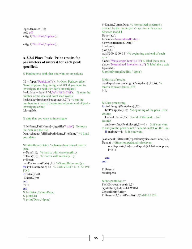
95

legend(names{:}); hold off set(gcf,'NextPlot','replace'); set(gcf,'NextPlot','replace');

A.3.2.4 Place Peak: Print results for parameters of interest for each peak specified.

% Parameters: peak that you want to investigate fid = fopen('Peak2.txt','r'); % Open Peak.txt (doc: Name of peaks, beginning, end, 0/1 if you want to investigate the peak (0= don't investigate)) Peakplace = fscanf(fid,'%*s %f %f %f'); % scan the number of the doc and don't scan words Peakplace=[reshape(Peakplace,3,2)]'; % put the numbers in a matrix (beginning of peak- end of peak-investigate or not) fclose(fid); % data that you want to investigate [FileName,PathName]=uigetfile('*.xlsx') %choose the Path and the file Data=xlsread(fullfile(PathName,FileName));% Load your datas %Data=flipud(Data); %change direction of matrix Data a=Data(:,1); % matrix with wavelength...x b=Data(:,2); % matrix with intensity ...y a=fix(a); maxData=max(Data(:,2)); %%maxData=max(y) for i=1:Data(end,2) do % CONVERTS NEGATIVE TO 0 if Data(i,2)<0 Data(i,2)=0 end i=i+1 end % b=Data(:,2)/maxData; % plot(a,b) % print('Data','-dpng')

b=Data(:,2)/maxData; % normalized spectrum : divided by the maximym -> spectra with values between 0 and 1 Data=[a,b]; filename='NormalizedF.xlsx' xlswrite(filename, Data) h1=figure; plot(a,b); axis([500 1500 0 1]) % beginning and end of each axis xlabel('Wavelength (cm^{-1})') % label the x axis ylabel('Normalized Intensity (a.u)') % label the y axis figure(h1) % print(NormalizedInt, '-dpng') %Matrix of results resultspeak=zeros(length(Peakplace(:,2)),6); % matrix to save results--6?? i=1; % Data processing for i=1:length(Peakplace(:,2)); K=Peakplace(i,1); %beginning of the peak ..first column L=Peakplace(i,2); % end of the peak ...2nd column analyze=find(Peakplace(i,3)==1); % if you want to analyze the peak or not : depend on 0/1 on the line if analyze==1; % if you want [valuepeak,FitResults]=peakanalyziselevenLana(K,L,Data,a) ; %function peakanalysiseleven resultspeak(i,1:6)=resultspeak(i,1:6)+valuepeak; i=i+1; end end FitResults resultspeak %PhospahteRatio= FWHM=resultspeak(1,5); crystallinityIndex=1/FWHM CrystallinityRatio= FitResults(2,5)/FitResults(1,5)%1030:1020

Documents

Multi-scale Assessment of Bone Mechanics and the Mineral