Embed Size (px)
Citation preview

NeuroImage 62 (2012) 48–58
Contents lists available at SciVerse ScienceDirect
NeuroImage
j ourna l homepage: www.e lsev ie r .com/ locate /yn img
Multi-scale classification of disease using structural MRI and wavelet transform
Kerstin Hackmack a,b,⁎, Friedemann Paul c,e, Martin Weygandt a,b,c,Carsten Allefeld a,b, John-Dylan Haynes a,b,c,d,⁎and The Alzheimer's Disease Neuroimaging Initiative 1
a Bernstein Center for Computational Neuroscience, Charité—Universitätsmedizin Berlin, Berlin, Germanyb Berlin Center for Advanced Neuroimaging, Charité—Universitätsmedizin Berlin, Berlin, Germanyc NeuroCure Clinical Research Center, Charité—Universitätsmedizin Berlin, Berlin, Germanyd Berlin School of Mind and Brain, Humboldt-Universität zu Berlin, Berlin, Germanye Experimental and Clinical Research Center, Max Delbrueck Center for Molecular Medicine, Berlin, Germany
Abbreviations: dt-CWT, dual-tree complex wavelet tnance imaging; MS, multiple sclerosis; NABT, normalsupport vector machine.⁎ Corresponding authors at: Bernstein Center for
Charité—Universitätsmedizin Berlin, Haus 6, PhilippstrFax: +49 30 209 367 69.
E-mail addresses: [email protected]@charite.de (F. Paul), martin.weygandt(M. Weygandt), [email protected] (C. Alle(J-D. Haynes).
1 Data used in the Supplementary material of this aAlzheimer's Disease Neuroimaging Initiative (ADNI) daedu/ADNI). As such, the investigators within the ADNIimplementation of ADNI and/or provided data but didwriting of this report. The complete list of ADNI invhttp://www.loni.ucla.edu/ADNI/Collaboration/ADNI Aut
1053-8119/$ – see front matter © 2012 Elsevier Inc. Alldoi:10.1016/j.neuroimage.2012.05.022
a b s t r a c t
a r t i c l e i n f oArticle history:Accepted 9 May 2012Available online 15 May 2012
Keywords:Multi-scale classificationMultiple sclerosisStructural MRISupport vector machineWavelet transform
Recently, multivariate analysis algorithms have become a popular tool to diagnose neurological diseasesbased on neuroimaging data. Most studies, however, are biased for one specific scale, namely the scalegiven by the spatial resolution (i.e. dimension) of the data. In the present study, we propose to use thedual-tree complex wavelet transform to extract information on different spatial scales from structural MRIdata and show its relevance for disease classification. Based on the magnitude representation of the complexwavelet coefficients calculated from the MR images, we identified a new class of features taking scale, direc-tionality and potentially local information into account simultaneously. By using a linear support vector ma-chine, these features were shown to discriminate significantly between spatially normalized MR images of 41patients suffering from multiple sclerosis and 26 healthy controls. Interestingly, the decoding accuracies var-ied strongly among the different scales and it turned out that scales containing low frequency informationwere partly superior to scales containing high frequency information. Usually, this type of information isneglected since most decoding studies use only the original scale of the data. In conclusion, our proposedmethod has not only a high potential to assist in the diagnostic process of multiple sclerosis, but can be ap-plied to other diseases or general decoding problems in structural or functional MRI.
© 2012 Elsevier Inc. All rights reserved.
Introduction
In recent years, multivariate analysis algorithms have become apopular tool to diagnose neurological or psychiatric diseases basedon structural or functional MRI data (Ashburner and Klöppel, 2011;Koutsouleris et al., 2009; Weygandt et al., 2011). The main challengehere lies in the identification of features which provide most
ransform; MRI, magnetic reso--appearing brain tissue; SVM,
Computational Neuroscience,. 13, 10115 Berlin, Germany.
(K. Hackmack),@bccn-berlin.defeld), [email protected]
rticle were obtained from theta base (http://www.loni.ucla.contributed to the design andnot participate in analysis or
estigators can be found here:horship list.pdf.
rights reserved.
information about the particular disease (so-called ‘disease signa-tures’). Features used in previous studies include local or global inten-sity patterns (e.g. Klöppel et al., 2008b; Weygandt et al., 2011) as wellas geometric and surface-based features (Ecker et al., 2010; Yotter etal., 2011). Most studies, however, are biased for specific scales, name-ly the scale given by the spatial resolution of the data. Although it iswell known that the brain is hierarchically organized at different spa-tial scales, ranging from individual neurons over cortical columns tolarger functional brain areas, the interplay between these spatialscales has been little addressed. This limitation can partly be over-come by using wavelets which provide a powerful means to analyzethe patterning of complex data on different scales (Sajda et al.,2002). By this, wavelets allow “zooming in” at different spatial scalesand thus can be interpreted as a form of dimensionality reduction.
A wavelet is a small wave-like oscillation which is used to decom-pose a signal with respect to scaled and translated versions of it. Incontrast to sine waves used as basis functions in the Fourier trans-form, wavelets are of limited duration and therefore allow for locali-zation in scale and space (Graps, 1995). By this, the wavelettransform provides a natural adaptability to local signal propertiesand non-stationary signals and thus can be used to analyze orienteddiscontinuities (i.e. directionality) such as edges or surfaces in the

49K. Hackmack et al. / NeuroImage 62 (2012) 48–58
data (Selesnick et al., 2005). Intuitively, the wavelet transform can beseen as a way of decomposing the energy of a signal into a hierarchi-cally organized set of scales (Bullmore et al., 2004). High frequencycomponents of the energy are represented by wavelet coefficients atfine scales, whereas low frequency components can be found atcoarse scales. For an introduction into wavelets, please refer toDaubechies (1992), Graps (1995) or Mallat (2008). The multi-resolution property of the wavelet transform has been used in a vari-ety of applications including functional MRI analysis (for a review seeBullmore et al., 2004 or Van De Ville et al., 2006). In the medical con-text, wavelets have been used as a way to discriminate betweenhealthy and pathological tissue (e.g. tumor cells or lesions; Antel etal., 2003; Castellano et al., 2004; Zhang et al., 2008). However, thesestudies were mostly based on 2-dimensional medical images anddid not focus on the importance of different spatial scales in dis-tinguishing the tissue classes. Although multi-scale representationsof medical data promise a rich source of information for disease clas-sification, we are not aware of any study investigating the impact ofdifferent scales in decoding a disease.
One of the most common neurological diseases is multiple sclero-sis (MS), which has only barely been investigated within the contextof multivariate analysis algorithms. MS is an autoimmune disease thataffects the central nervous system leading to inflammation, demye-lination and neurodegeneration of brain tissue (Compston andColes, 2008). These alterations can cause a number of neurologicalproblems such as impaired function of the motor, somatosensory orvisual system. Since the introduction of the McDonald criteria(McDonald et al., 2001), conventional MRI has become one of thecornerstones in diagnosing MS. Radiologically, MS is mainly char-acterized by three neurobiological markers: focal inflammatory le-sions, neurodegeneration and subtle tissue alterations (Filippi andRocca, 2005). In contrast to lesions, regional neurodegenerationand subtle tissue alterations usually remain undetected in conven-tional MRI and are therefore termed normal-appearing brain tissue(NABT; Filippi et al., 2004). In two recent studies of our group,however, we have shown that local intensity patterns extractedfrom NABT areas contain information about disease status(Weygandt et al., 2011) and symptom severity (Hackmack et al.,2012). These studies, however, were only based on the originalsize of the MR volumes and therefore did not cover multi-scaleinformation.
Here, we use wavelets to investigate the significance of differentscales in discriminating between MR images of MS patients andhealthy controls. For the wavelet decomposition, we used the dual-tree complex wavelet transform (Kingsbury, 2001; Selesnick et al.,2005) which has the advantage of being approximately shift-invariant and directionally selective. For 3-dimensional MR volumes,28 different directions can be isolated. This means that on eachscale 28 orientation subbands (which are again 3-dimensional vol-umes) are generated with each capturing one specific direction inthe data. Based on the magnitude of the complex wavelet coefficientsin each of the subbands, we used two strategies to investigate direc-tionality at different scales. In the first analysis (‘global analysis of an-isotropy’), we calculated for each subject the overall energy containedin each of the subbands at one particular scale. This type of features(‘global wavelet features’) captured scale and directionality informa-tion, but disregarded local information by assessing the energythroughout all brain locations. For each scale, it leads to one final di-agnosis per subject. In contrast, in the second analysis (‘local analysisof anisotropy’) we used the local pattern of directionality by includingthe position within the subbands. These features (‘local wavelet fea-tures’) allow for a precise mapping of relevant regions. Both analyseswere conducted for each scale separately. To classify between globalor local wavelet features of MS patients and healthy controls, weused a linear support vector machine (Cortes and Vapnik, 1995;Shawe-Taylor and Christianini, 2000).
Materials and methods
Patients
We reanalyzed the data of 41 patients (21 females and 20 males;age, median (MD)=34, range 19–51) with clinically definite MS (re-lapsing-remitting type; McDonald et al., 2001) and 26 age and gendermatched healthy controls (14 females, 12 males; age, MD=36.5,range 23–57) already used in two previous studies of our group(Hackmack et al., 2012; Weygandt et al., 2011). Disease duration wason average 84.0 months (standard deviation (SD)=76.3). Mean T1 le-sion load was 1872.2 mm3 (SD=6279.5; ‘black holes’) and T2 lesionload was 5224.0 mm3 (SD=4117.8). The patients exhibited a mild tomoderate score on the Expanded Disability Status Scale (EDSS;Kurtzke, 1983; MD=2, range 0–7). Additionally, patients were scoredon the Multiple Sclerosis Functional Composite (MSFC; Cutter et al.,1999) and subtests 9-Hole Peg Test (9-HPT; mean (M)=19.4,SD=3.3), Timed Walk Test (TWT; M=5.0, SD=1.7), and Paced Audi-tory Serial Addition Test (PASAT; M=52.4, SD=9.1). Consent wasobtained according to the Declaration of Helsinki, and the studywas ap-proved by the research ethics committee of the Charité—Uni-versitätsmedizin Berlin. All subjects gave written informed consent.
Magnetic resonance imaging
Whole-brain high-resolution 3dimensional T1weighted images(MPRAGE, TR 2110 ms, TE 4.38 ms, TI 1100 ms, flip angle 15°, resolu-tion 1×1×1 mm) and T2weighted fluid-attenuated inversion recov-ery sequence images (TIRM, TR 10000 ms, TE 108 ms, TI 2500 ms,resolution 1×1×3 mm, 44 contiguous axial slices) were acquiredusing a 1.5 Tesla MRI (Magnetom Sonata, Siemens, Erlangen, Germa-ny) with an 8-channel standard head coil. Lesion load for MPRAGEand TIRM images was routinely measured using the MedX v.3.4.3software package (Sensor Systems Inc., Sterling, VA, USA). Lesionload of TIRM images was additionally measured using in-house soft-ware (Weygandt et al., 2011).
Preprocessing
In accordance with our previous studies (Hackmack et al., 2012;Weygandt et al., 2011), several preprocessing steps were performed.First, a clinician used in-house software to conduct a lesion mappingbased on individual TIRM images. To be as conservative as possible,the clinician was instructed to mark any hyperintensities visible inthe TIRM images and not only oval lesions as it is common in clinicalpractice. Next, correction of field inhomogeneities, coregistration ofhigh-resolution MPRAGE and TIRM images, and spatial normalizationof these high-resolution images to the Montreal Neurological Insti-tute (MNI) 152 brain template (voxel resolution: 2×2×2 mm)were conducted using SPM5 (Wellcome Trust Centre for Neuroimag-ing, Institute of Neurology, UCL, London, http://www.fil.ion.ucl.ac.uk/spm). The spatial normalization parameters for the MPRAGE imageswere estimated by the ‘unified segmentation approach’ (Ashburnerand Friston, 2005) and then applied to the co-registered TIRM imagesas well as to individual lesion masks. Importantly, lesion areas identi-fied by the clinician were excluded to avoid lesion-mediated artifactsin the normalization routine. Finally, we obtained TIRM images fromall subjects as well as their individual lesion masks in MNI space (vol-ume size: 79×95×69; voxel size: 2×2×2 mm).
For the wavelet transformation, the spatial normalized TIRM im-ages were masked in three different ways (Fig. 1). First, all voxelswithin the SPM standard brain mask that were not cerebrospinalfluid (CSF) with a probability of more than 0.8 (based on SPM CSFprior map) were included (referred to as brain mask). The rather con-servative threshold of 0.8 was chosen to avoid misinterpretation oftissue-free voxels as brain tissue. Based on the brain mask, we created

Fig. 1. Overview of data processing. Raw MR volumes were normalized to the Montreal Neurological Institute (MNI) template and then masked by one of the three masks: brainmask (BM), lesion mask (LES) or normal-appearing brain matter mask (NABT). For the resulting MR volumes, we calculated a 6-level dual-tree complex wavelet transform (dt-CWT) resulting in 6 different scales and 28 oriented subbands (see Fig. 2) per scale, where each subband is again a 3-dimensional volume containing a different number of voxelsdepending on scale. For illustration, we here show an example of a 3-level dt-CWT of a 2-dimensional MR image resulting in 3 scales and 6 subbands per scale. Each subband isolatesa specific direction in the image (±15°, ±45°, ±75°). Based on the magnitude representation of the wavelet coefficients, we extracted either global wavelet features (feature ex-traction I) or local wavelet features (feature extraction II). For the global wavelet features, we calculated the log-energy for each subband within a particular scale (Figure: Scale I).Please note that the log-energy is computed across all positions within a subband. We then conducted a classification analysis (‘global analysis of anisotropy’) for each scale sep-arately to discriminate between the features of MS patients (MS) and healthy controls (HC). For the local wavelet features, we extracted the magnitude at one particular location(i.e. voxel position) across all subbands within one scale. Thus, the features depend not only on the scale but also on the position within the subband and therefore represent localdirectional information. The features were then used as above by a classification analysis (‘local analysis of anisotropy’) to separate between the two groups. Importantly, the clas-sification analysis was not only conducted separately for each scale, but also for each voxel position.
50 K. Hackmack et al. / NeuroImage 62 (2012) 48–58
two further masks: (1) lesion mask and (2) normal-appearing brainmatter (NABT) mask. Whereas the lesion mask includes only thatmatter where at least one person had a lesion, the NABT mask in-cludes only that matter where none of the MS patients had a lesion.Please note that within the lesion mask only 6.83% of voxels acrossall subjects were actually lesioned. The lesion and NABT mask togeth-er add up to the brain mask. Only image intensity values within themask (brain, lesion or NABT) were used for calculating the waveletcoefficients, all other values were set to zero. Since the masks wereequal for MS patients and healthy controls, boundary effects intro-duced in the decomposition due to prior masking are equal for bothgroups and are therefore not relevant for classification. In Supple-mentary Table 1, results without prior masking are depicted, whichshow significant results for scales I, III and all scales together. To ac-count for different overall intensity levels the images were standard-ized within subjects by subtracting the mean and dividing by thestandard deviation of normal-appearing (i.e. non-lesional) brain tis-sue. This was done to ensure that a higher lesion load did not intro-duce any biases into the standardization. Since the waveletimplementation requires the image dimensions to be a power of 2,we filled the MR volumes with zeros until the next power of 2 isachieved (new volume size: 128×128×128).
To rule out that the results obtained for the discrimination of MSpatients and healthy controls relied on effects related to MS-relatedpreprocessing steps (i.e. lesion masking), we repeated the globaland local analyses of anisotropy for an MRI data set of 20 Alzheimer'spatients and 20 healthy controls obtained from the Alzheimer's Dis-ease Neuroimaging Initiative (ADNI) data base (see Supplementarymaterial and Supplementary Tables 7–8).
Wavelet decomposition
The discrete wavelet transform (DWT; Burrus et al., 1997;Daubechies, 1992; Graps, 1995; Mallat, 1989, 2008) is a powerfultool to handle signals at different scales. Within the DWT, a signal isbroken up into shifted and scaled versions of one original ‘mother-wavelet’. For 2- or 3-dimensional signals, this mother-wavelet is aspatial pattern and is usually required to have compact support andvanishing higher moments (Daubechies, 1988, 1992; Meyer, 1987).As a consequence of limited duration, wavelets allow for localizationin scale (i.e. frequency) and space and can therefore be used to ana-lyze local, spatial transients in the data such as edges or surfaces(Bullmore et al., 2004; Selesnick et al., 2005). This means that wave-lets allow capturing information at different spatial scales whilemaintaining locality. By this, the wavelet transform provides a hugeadvantage over the Fourier transform, which is only localized in fre-quency and thus cannot be used to analyze local patterns. Intuitively,the DWT allows for zooming in at particular scales of interest. Sincethe spatial resolution of the signal is reduced in each decompositionstep, the wavelet transform is also a form of dimensionality reduction.In this respect, the DWT can be viewed as a way to decompose the en-ergy of a signal over a hierarchy of scales distributed to different di-rections in the data (Bullmore et al., 2004). Computationally, theDWT can be implemented via a filter bank (Burrus et al., 1997),which provides a fast way to calculate the wavelet coefficients byusing an array of high and low pass filters.
The dual-tree complex wavelet transform (dt-CWT; Kingsbury,2001; Selesnick et al., 2005; MATLAB implementation can be foundhere: http://taco.poly.edu/WaveletSoftware/) is an improvement of

51K. Hackmack et al. / NeuroImage 62 (2012) 48–58
the DWT, which calculates the complex transform of a signal usingtwo real DWTs. The dt-CWT can then be represented by the matrixF=[Fh Fg], where the matrices Fh and Fg represent the real transforms.The complex wavelet coefficients of a real signal x are then given byFh ∙x+i ∙Fg ∙x. Thus, the first DWT gives the real part of the transform,and the second DWT the imaginary part. Both DWTs are implementedvia a filter bank, but use different sets of filters. However, the filtersare jointly designed to ensure that the overall transform is approxi-mately analytic (Selesnick et al., 2005). By this, the dt-CWT providestwo main advantages over the standard DWT: approximate shift-invariance and high direction selectivity in two and higher dimensions.
Shift-invariance means that the wavelet coefficients do not changewhen the signal is shifted in the time or space domain. Approximateshift-invariance, however, is realized at the cost of a redundancy of2d wavelet coefficients (d dimension; i.e. 8-times as many coefficientsare needed to represent a 3-dimensional MR image in the dual-treewavelet domain).
Direction selectivity allows for an isolation of different directionsin the signal, for example edges in images or surfaces in volumes.For a 2-dimensional image, 6 different directions can be isolated(±15°, ±45°, ±75°; Fig. 1), whereas for a 3-dimensional volume,28 different orientations can be segregated (Fig. 2). Importantly,these orientations are present at each spatial scale. Please note thatthe standard DWT can only distinguish between horizontal and verti-cal directions, but not between diagonal directions (so-called ‘check-erboard artifact’). In Supplementary Fig. 1, Fourier transform,
Fig. 2. 3-dimensional isosurfaces. The real part of the complex isosurfaces given by the dualresponds to a specific orientation. These illustrations were made with the same software wWaveletSoftware/).
standard DWT and dt-CWT are compared with respect to their effecton a 2-dimensional image.
For each subject, we calculated a 6-level dt-CWT based on thepreprocessed 3-dimensional MR volumes resulting in 6 differentscales (from scales I to VI, VI describing the coarsest) and 28 orientedsubbands per scale. These subbands are again 3-dimensional vol-umes, which contain a certain number of voxels depending on thescale. The number of voxels refers to the spatial resolution of the par-ticular scale. In our case, the 28 orientation subbands at the first scalehave a resolution of 64×64×64, the orientation subbands at the sec-ond scale have a resolution of 32×32×32 and so on. Each voxel with-in a subband is described by a complex wavelet coefficient which isprovided by the dt-CWT. Here, we use the magnitude representationof the complex wavelet coefficients since we are interested in direc-tionality at different scales and the relative magnitude can be seenas a marker of directionality: a larger magnitude indicates the pres-ence of structures of a particular scale and orientation in the data(e.g. edges or surfaces). Consequently, the magnitude of each voxeldepends on the scale, the orientation and the position of the voxelwithin the subband. Please note that the voxel size differs betweenthe different spatial scales and thus the term voxel is not restrictedto the voxels in the raw MRI data but is generally meant for ‘volumeelement’ (where the size is determined by the scale).
For decomposition, we used the Kingsbury Q-filters which are animproved version of the original dt-CWT filters that have better orthog-onality and symmetry properties (Kingsbury, 2000). As mentioned
-tree complex wavelet transform is shown for each subband, where each subband cor-e used for calculating the dual-tree complex wavelet transform (http://taco.poly.edu/
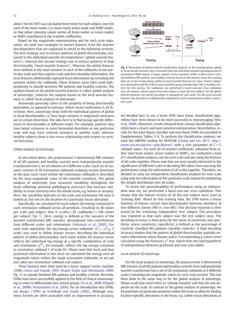
Fig. 3. Illustration of pattern-based classification analysis. In the training phase, globalor local wavelet features were extracted from the individual wavelet decompositions ofnormalized TIRM images. A linear support vector machine (SVM) is then used to clas-sify between MS patients and healthy controls based on the features from the trainingdata set. In the testing phase, global or local wavelet features of a new ‘unseen’ subjectare represented and the SVM is used to predict group membership (MS or healthy con-trol) for this person. For validation, we performed a leave-one-out cross-validationover all subjects, which means that each subject is once the test subject. For the globalwavelet features, the whole procedure is repeated for each scale. For the local waveletfeatures, the procedure is additionally repeated for each voxel position within a partic-ular scale.
52 K. Hackmack et al. / NeuroImage 62 (2012) 48–58
above, the dt-CWTwas calculated three times for each subject, once foreach of the three masks (i.e. brain mask, lesion mask and NABT mask),so that either intensity values within all brain matter or lesion matteror NABT contributed to the wavelet coefficients.
Based on the magnitude representation and for each scale sepa-rately, we used two strategies to extract features from the waveletdecomposition that are explained in detail in the following sections.The first strategy was to extract patterns of global directionality con-tained in the individual wavelet decompositions (‘global wavelet fea-tures’), whereas the second strategy was to extract patterns of localdirectionality (‘local wavelet features’). Whereas the global featureswere defined as the total variance in each of the subbands at one par-ticular scale and thus capture scale and directionality information, thelocal features additionally captured local information by including theposition within the subbands. These features were then used inde-pendently to classify between MS patients and healthy controls. Theanalysis based on the global wavelet features is called ‘global analysisof anisotropy’, whereas the analysis based on the local wavelet fea-tures is called ‘local analysis of anisotropy’.
Anisotropy generally refers to the property of being directionallydependent, as opposed to isotropy, which means uniformity in all di-rections. Here, anisotropy deals with the individual pattern of globalor local directionality, i.e. how large variance or magnitude measuresare in certain directions. The idea here is to find group-specific differ-ences in directionality at different scales. For example, patients mayhave larger variances in more horizontal directions at one particularscale and may have reduced variances at another scale, whereashealthy subjects show a vice-versa relationship with respect to verti-cal directions.
Global analysis of anisotropy
As described above, the preprocessed 3-dimensional MR volumesof all MS patients and healthy controls were independently wavelettransformed into a set of volumes at 6 different scales. Each set of vol-umes consists of 28 orientation subbands isolating certain directionsin the data. Each voxel within the orientation subbands is describedby the local magnitude value of the wavelet transform. The globalanalysis of anisotropy now measures variability throughout thebrain reflecting potential pathological processes that increase vari-ability in tissue intensity over the whole-brain, e.g. lesions or atrophy.Here, the variability depends on the scale and orientation the data islooked at, but not on the location of a particular tissue alteration.
Specifically, we calculated for each subject the energy contained ineach orientation subband across all positions (resulting in 28 valuesper scale and subject, thus 6 (scales)∗28 (subbands)=168 valuesper subject; Fig. 1). Here, energy is defined as the variance of thewavelet transformed MR volumes, decomposed into contributionsfrom different scales and orientations (Selesnick et al., 2005). Foreach scale separately, the log-energy across subbands (eS1,…,eS28, Sscale) was used to define feature vectors describing the individualpattern of global directionality. Each value within the feature vectorreflects the individual log-energy at a specific combination of scaleand orientation (eIV1, for example, reflects the log-energy containedin orientation subband 1 of scale IV). Please note that local and thuspositional information is lost since we calculated the energy over allmagnitude values within the single orientation subbands, so we getone value per orientation subband and subject.
These features were then used by a linear support vector machine(SVM; Cortes and Vapnik, 1995; Shawe-Taylor and Christianini, 2000;Fig. 3) to classify between MS patients and healthy controls. Recently,SVMs have been successfully applied in the field of clinical neuroimag-ing in order to differentiate two clinical groups (Fu et al., 2008; Klöppelet al., 2008b; Koutsouleris et al., 2009). For an introduction into SVMs,see Burges (1998) or Schölkopf and Smola (2002). Although non-linear kernels are often associated with an improvement in accuracy,
we decided here to use a linear SVM since linear classification algo-rithms have been shown to be most successful in neuroimaging (Muret al., 2009).Moreover, results obtained froma linear classification algo-rithmhave a clearer andmore intuitive interpretation. Nevertheless, re-sults for the naive Bayes classifier and non-linear SVMs are provided inSupplementary Tables 2–4. To perform the classification analyses, weused the LIBSVM toolbox for MATLAB (Chang and Lin, 2011; http://www.csie.ntu.edu.tw/~cjlin/libsvm/) with a cost parameter of C=1(default value). For each set of wavelet coefficients (obtained from ei-ther total brain matter, lesion matter or NABT), we conducted a totalof 7 classification analyses, one for each scale and one using the featuresof all scales together. Please note that we were mostly interested in thesignificance of different scales in decodingMS rather than assessing theperformance using the information of all scales together. Therefore, wedecided to carry out independent classification analyses for each scaleusing only the information of this particular scale instead of consideringthe weight distribution over all scales.
To assess the generalizability of performance using an indepen-dent data set, we performed a leave-one-out cross-validation. Thismeans that the feature vectors of all but one subject were used as‘training data’. Based on this training data, the SVM learns a linearfunction of feature vectors that discriminates between members oftwo different classes (MS vs. non-MS). This decision function is thentested on the remaining, independent ‘test’ subject. This procedurewas repeated so that each subject was the test subject once. Thedecoding accuracy is then given by the mean of sensitivity and spec-ificity, where sensitivity (specificity) is defined as the percentage ofcorrectly classified MS patients (healthy controls). A high decodingaccuracy implies that the pattern of global directionality spatially en-codes information about disease status. Corresponding p-values werecalculated using the Pearson's χ2 test, which tests the null hypothesisof independence between predicted and true class labels.
Local analysis of anisotropy
For the local analysis of anisotropy, the preprocessed 3-dimensionalMR volumes of allMSpatients andhealthy controlswere independentlywavelet transformed into a set of 28 orientation subbands at 6 differentscales containing the magnitude values for each voxel position. This hasbeen done in the same way as for the global analysis of anisotropy.Please recall that voxel refers to ‘volume element’ and that the size de-pends on the scale. In contrast to the global analysis of anisotropy, wefocusedhere on particular positionswithin the brain to allow forfindinglocation-specific alterations in the brain, e.g. subtle tissue alterations at

53K. Hackmack et al. / NeuroImage 62 (2012) 48–58
a particular position that are inmost patients present, but not in healthycontrols.
Specifically, we used the voxel-wise magnitude values instead of aglobal variance marker for discriminating between MS patients andhealthy controls. Thus, we extracted the magnitude value at thesame location (i.e. same voxel position) across all 28 subbands forone particular scale (Fig. 1). The feature vectors therefore dependnot only on scale but also on the voxel position (eS1i,…,eS28i, S scale,voxel i) and can be interpreted as the ‘signal energy’ contained in aspecific combination of scale, orientation and location (Selesnick etal., 2005). This means that our algorithm searches across the sub-bands at one particular scale for local directionality patterns informa-tive about the clinical status
Based on the feature vectors, we conducted again a linear SVM toclassify between MS patients and healthy controls (Fig. 3). As above,results were validated using a leave-one-out cross-validation andcorresponding p-values were calculated using the Pearson's χ2 test,which tests the null hypothesis of independence between predictedand true class labels. Please note that the number of voxels and thusthe number of classification analyses varied between the three brainmatter types and the different scales (i.e. up to 643 analyses forscale I, up to 323 analyses for scale II and so on). Voxels having zeromagnitude were excluded. The high number of classification analysesmakes it necessary to correct for multiple comparisons, a statisticalproblem originating from the fact that if a statistical test is often repeat-ed, it is likely to observe some false positives. To account for the multi-ple comparison problem in this study, we report only voxel coordinatesthat exhibit a significant decoding accuracy on a Bonferroni-correctedlevel of pb0.05, which means that the significance level of 0.05 was di-vided by the number of classification analyses for either total brainmat-ter, lesion matter or NABT. For example, only voxel coordinates with
Fig. 4. Results of the global analysis of anisotropy. In (A) the difference of mean feature vecshown for total brain matter, lesion matter and normal-appearing brain matter (NABT), respSensitivity, specificity and decoding accuracy of corresponding classification analyses are givaccuracies are marked by one or two stars (*: pb0.05; **: pb0.001).
pb0.05/57508 (equivalent to pb0.05, Bonferroni corrected) arereported for brain matter. This rather conservative threshold was cho-sen to increase the specificity of the analyses. Other correctionmethodscommonly used in the neuroimaging literature are false discovery ratecontrol, family wise error correction and permutation testing (NicholsandHayasaka, 2003). By not reducing the search space prior to the anal-ysis, this approach allows for an unbiased whole-brain informationmapping.
Results
Global analysis of anisotropy
For the global analysis of anisotropy, the difference between meanfeature vectors of MS patients and healthy controls, respectively, isplotted in Fig. 4A, separately for total brain matter, lesion matterand NABT. Interestingly, their difference varied with respect to scaleand orientation. For most subbands and especially for total brain mat-ter and lesion matter, the MS patients tend to have higher energyvalues. Geometrically, this means that the MR volumes of the patientsare characterized by more variability or ‘roughness’ (e.g. caused bythe hyperintensity of lesions) than the MR volumes of the controls.For NABT, however, also some negative peaks, where MS patientshave lower energy values, could be identified. As expected, the differ-ences were most apparent for lesion matter. Correspondingly,decoding accuracies were largest for lesion matter and varied herebetween 81.85% and 97.56% with a peak in scale II. For total brainmatter, decoding accuracies ranged from 75.56% to 83.07% with apeak in scale III. The differences between the scales were not as strongas for the lesion matter, though. For NABT, the decoding accuracieswere smaller, but still significant for scales I, III, IV, V and all scales
tors between MS patients and healthy controls (red) and the standard error (black) isectively. For each scale, the difference of mean log-energy of all 28 subbands is shown.en in (B), separately for each scale and once for all scales together. Significant decoding
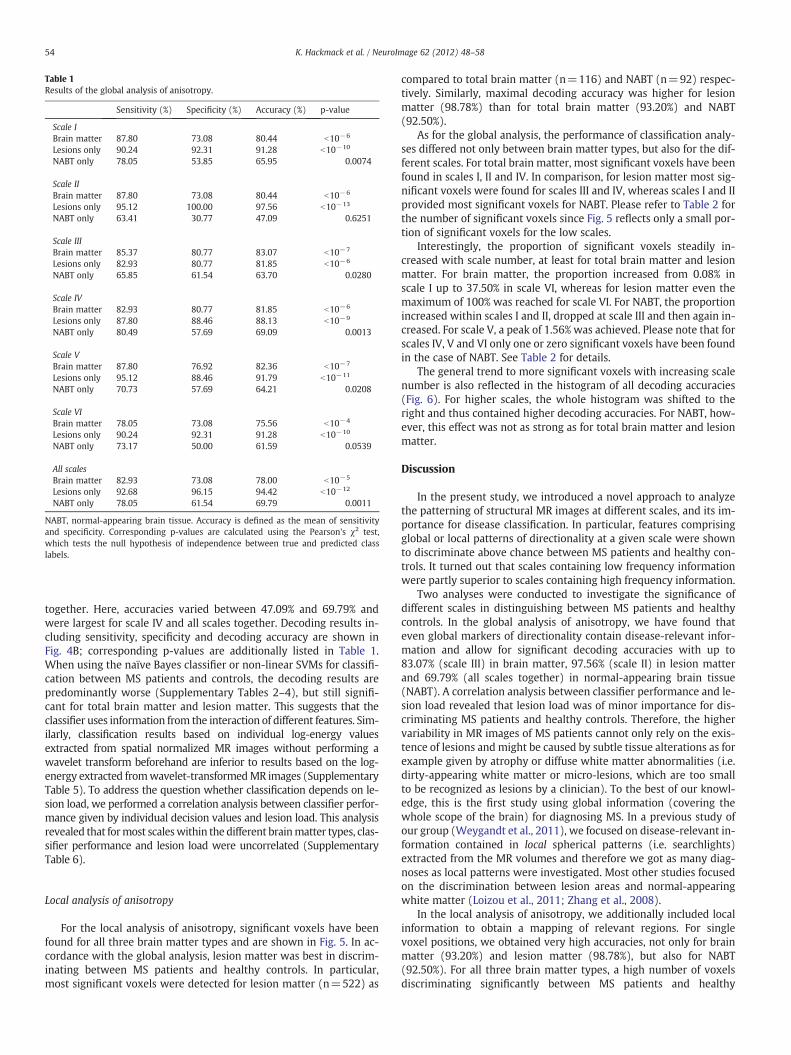
Table 1Results of the global analysis of anisotropy.
Sensitivity (%) Specificity (%) Accuracy (%) p-value
Scale IBrain matter 87.80 73.08 80.44 b10−6
Lesions only 90.24 92.31 91.28 b10−10
NABT only 78.05 53.85 65.95 0.0074
Scale IIBrain matter 87.80 73.08 80.44 b10−6
Lesions only 95.12 100.00 97.56 b10−13
NABT only 63.41 30.77 47.09 0.6251
Scale IIIBrain matter 85.37 80.77 83.07 b10−7
Lesions only 82.93 80.77 81.85 b10−6
NABT only 65.85 61.54 63.70 0.0280
Scale IVBrain matter 82.93 80.77 81.85 b10−6
Lesions only 87.80 88.46 88.13 b10−9
NABT only 80.49 57.69 69.09 0.0013
Scale VBrain matter 87.80 76.92 82.36 b10−7
Lesions only 95.12 88.46 91.79 b10−11
NABT only 70.73 57.69 64.21 0.0208
Scale VIBrain matter 78.05 73.08 75.56 b10−4
Lesions only 90.24 92.31 91.28 b10−10
NABT only 73.17 50.00 61.59 0.0539
All scalesBrain matter 82.93 73.08 78.00 b10−5
Lesions only 92.68 96.15 94.42 b10−12
NABT only 78.05 61.54 69.79 0.0011
NABT, normal-appearing brain tissue. Accuracy is defined as the mean of sensitivityand specificity. Corresponding p-values are calculated using the Pearson's χ2 test,which tests the null hypothesis of independence between true and predicted classlabels.
54 K. Hackmack et al. / NeuroImage 62 (2012) 48–58
together. Here, accuracies varied between 47.09% and 69.79% andwere largest for scale IV and all scales together. Decoding results in-cluding sensitivity, specificity and decoding accuracy are shown inFig. 4B; corresponding p-values are additionally listed in Table 1.When using the naïve Bayes classifier or non-linear SVMs for classifi-cation between MS patients and controls, the decoding results arepredominantly worse (Supplementary Tables 2–4), but still signifi-cant for total brain matter and lesion matter. This suggests that theclassifier uses information from the interaction of different features. Sim-ilarly, classification results based on individual log-energy valuesextracted from spatial normalized MR images without performing awavelet transform beforehand are inferior to results based on the log-energy extracted fromwavelet-transformedMR images (SupplementaryTable 5). To address the question whether classification depends on le-sion load, we performed a correlation analysis between classifier perfor-mance given by individual decision values and lesion load. This analysisrevealed that formost scaleswithin the different brainmatter types, clas-sifier performance and lesion load were uncorrelated (SupplementaryTable 6).
Local analysis of anisotropy
For the local analysis of anisotropy, significant voxels have beenfound for all three brain matter types and are shown in Fig. 5. In ac-cordance with the global analysis, lesion matter was best in discrim-inating between MS patients and healthy controls. In particular,most significant voxels were detected for lesion matter (n=522) as
compared to total brain matter (n=116) and NABT (n=92) respec-tively. Similarly, maximal decoding accuracy was higher for lesionmatter (98.78%) than for total brain matter (93.20%) and NABT(92.50%).
As for the global analysis, the performance of classification analy-ses differed not only between brain matter types, but also for the dif-ferent scales. For total brain matter, most significant voxels have beenfound in scales I, II and IV. In comparison, for lesion matter most sig-nificant voxels were found for scales III and IV, whereas scales I and IIprovided most significant voxels for NABT. Please refer to Table 2 forthe number of significant voxels since Fig. 5 reflects only a small por-tion of significant voxels for the low scales.
Interestingly, the proportion of significant voxels steadily in-creased with scale number, at least for total brain matter and lesionmatter. For brain matter, the proportion increased from 0.08% inscale I up to 37.50% in scale VI, whereas for lesion matter even themaximum of 100% was reached for scale VI. For NABT, the proportionincreased within scales I and II, dropped at scale III and then again in-creased. For scale V, a peak of 1.56% was achieved. Please note that forscales IV, V and VI only one or zero significant voxels have been foundin the case of NABT. See Table 2 for details.
The general trend to more significant voxels with increasing scalenumber is also reflected in the histogram of all decoding accuracies(Fig. 6). For higher scales, the whole histogram was shifted to theright and thus contained higher decoding accuracies. For NABT, how-ever, this effect was not as strong as for total brain matter and lesionmatter.
Discussion
In the present study, we introduced a novel approach to analyzethe patterning of structural MR images at different scales, and its im-portance for disease classification. In particular, features comprisingglobal or local patterns of directionality at a given scale were shownto discriminate above chance between MS patients and healthy con-trols. It turned out that scales containing low frequency informationwere partly superior to scales containing high frequency information.
Two analyses were conducted to investigate the significance ofdifferent scales in distinguishing between MS patients and healthycontrols. In the global analysis of anisotropy, we have found thateven global markers of directionality contain disease-relevant infor-mation and allow for significant decoding accuracies with up to83.07% (scale III) in brain matter, 97.56% (scale II) in lesion matterand 69.79% (all scales together) in normal-appearing brain tissue(NABT). A correlation analysis between classifier performance and le-sion load revealed that lesion load was of minor importance for dis-criminating MS patients and healthy controls. Therefore, the highervariability in MR images of MS patients cannot only rely on the exis-tence of lesions and might be caused by subtle tissue alterations as forexample given by atrophy or diffuse white matter abnormalities (i.e.dirty-appearing white matter or micro-lesions, which are too smallto be recognized as lesions by a clinician). To the best of our knowl-edge, this is the first study using global information (covering thewhole scope of the brain) for diagnosing MS. In a previous study ofour group (Weygandt et al., 2011), we focused on disease-relevant in-formation contained in local spherical patterns (i.e. searchlights)extracted from the MR volumes and therefore we got as many diag-noses as local patterns were investigated. Most other studies focusedon the discrimination between lesion areas and normal-appearingwhite matter (Loizou et al., 2011; Zhang et al., 2008).
In the local analysis of anisotropy, we additionally included localinformation to obtain a mapping of relevant regions. For singlevoxel positions, we obtained very high accuracies, not only for brainmatter (93.20%) and lesion matter (98.78%), but also for NABT(92.50%). For all three brain matter types, a high number of voxelsdiscriminating significantly between MS patients and healthy
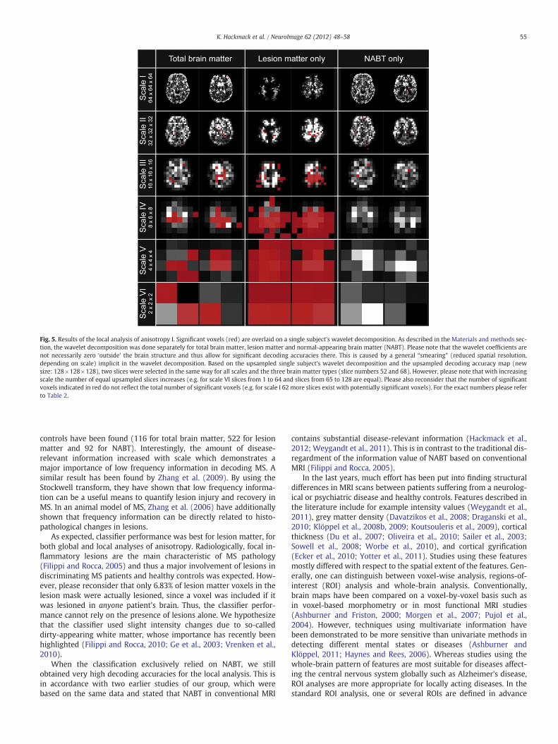
Fig. 5. Results of the local analysis of anisotropy I. Significant voxels (red) are overlaid on a single subject's wavelet decomposition. As described in the Materials and methods sec-tion, the wavelet decomposition was done separately for total brain matter, lesion matter and normal-appearing brain matter (NABT). Please note that the wavelet coefficients arenot necessarily zero ‘outside’ the brain structure and thus allow for significant decoding accuracies there. This is caused by a general “smearing” (reduced spatial resolution,depending on scale) implicit in the wavelet decomposition. Based on the upsampled single subject's wavelet decomposition and the upsampled decoding accuracy map (newsize: 128×128×128), two slices were selected in the same way for all scales and the three brain matter types (slice numbers 52 and 68). However, please note that with increasingscale the number of equal upsampled slices increases (e.g. for scale VI slices from 1 to 64 and slices from 65 to 128 are equal). Please also reconsider that the number of significantvoxels indicated in red do not reflect the total number of significant voxels (e.g. for scale I 62 more slices exist with potentially significant voxels). For the exact numbers please referto Table 2.
55K. Hackmack et al. / NeuroImage 62 (2012) 48–58
controls have been found (116 for total brain matter, 522 for lesionmatter and 92 for NABT). Interestingly, the amount of disease-relevant information increased with scale which demonstrates amajor importance of low frequency information in decoding MS. Asimilar result has been found by Zhang et al. (2009). By using theStockwell transform, they have shown that low frequency informa-tion can be a useful means to quantify lesion injury and recovery inMS. In an animal model of MS, Zhang et al. (2006) have additionallyshown that frequency information can be directly related to histo-pathological changes in lesions.
As expected, classifier performance was best for lesion matter, forboth global and local analyses of anisotropy. Radiologically, focal in-flammatory lesions are the main characteristic of MS pathology(Filippi and Rocca, 2005) and thus a major involvement of lesions indiscriminating MS patients and healthy controls was expected. How-ever, please reconsider that only 6.83% of lesion matter voxels in thelesion mask were actually lesioned, since a voxel was included if itwas lesioned in anyone patient's brain. Thus, the classifier perfor-mance cannot rely on the presence of lesions alone. We hypothesizethat the classifier used slight intensity changes due to so-calleddirty-appearing white matter, whose importance has recently beenhighlighted (Filippi and Rocca, 2010; Ge et al., 2003; Vrenken et al.,2010).
When the classification exclusively relied on NABT, we stillobtained very high decoding accuracies for the local analysis. This isin accordance with two earlier studies of our group, which werebased on the same data and stated that NABT in conventional MRI
contains substantial disease-relevant information (Hackmack et al.,2012; Weygandt et al., 2011). This is in contrast to the traditional dis-regardment of the information value of NABT based on conventionalMRI (Filippi and Rocca, 2005).
In the last years, much effort has been put into finding structuraldifferences in MRI scans between patients suffering from a neurolog-ical or psychiatric disease and healthy controls. Features described inthe literature include for example intensity values (Weygandt et al.,2011), grey matter density (Davatzikos et al., 2008; Draganski et al.,2010; Klöppel et al., 2008b, 2009; Koutsouleris et al., 2009), corticalthickness (Du et al., 2007; Oliveira et al., 2010; Sailer et al., 2003;Sowell et al., 2008; Worbe et al., 2010), and cortical gyrification(Ecker et al., 2010; Yotter et al., 2011). Studies using these featuresmostly differed with respect to the spatial extent of the features. Gen-erally, one can distinguish between voxel-wise analysis, regions-of-interest (ROI) analysis and whole-brain analysis. Conventionally,brain maps have been compared on a voxel-by-voxel basis such asin voxel-based morphometry or in most functional MRI studies(Ashburner and Friston, 2000; Morgen et al., 2007; Pujol et al.,2004). However, techniques using multivariate information havebeen demonstrated to be more sensitive than univariate methods indetecting different mental states or diseases (Ashburner andKlöppel, 2011; Haynes and Rees, 2006). Whereas studies using thewhole-brain pattern of features are most suitable for diseases affect-ing the central nervous system globally such as Alzheimer's disease,ROI analyses are more appropriate for locally acting diseases. In thestandard ROI analysis, one or several ROIs are defined in advance
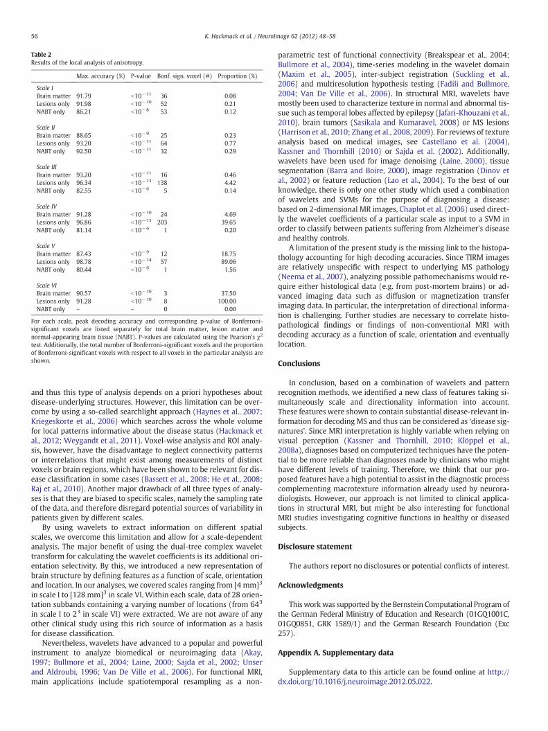
Table 2Results of the local analysis of anisotropy.
Max. accuracy (%) P-value Bonf. sign. voxel (#) Proportion (%)
Scale IBrain matter 91.79 b10−11 36 0.08Lesions only 91.98 b10−10 52 0.21NABT only 86.21 b10−8 53 0.12
Scale IIBrain matter 88.65 b10−9 25 0.23Lesions only 93.20 b10−11 64 0.77NABT only 92.50 b10−11 32 0.29
Scale IIIBrain matter 93.20 b10−11 16 0.46Lesions only 96.34 b10−13 138 4.42NABT only 82.55 b10−6 5 0.14
Scale IVBrain matter 91.28 b10−10 24 4.69Lesions only 96.86 b10−13 203 39.65NABT only 81.14 b10−6 1 0.20
Scale VBrain matter 87.43 b10−9 12 18.75Lesions only 98.78 b10−14 57 89.06NABT only 80.44 b10−6 1 1.56
Scale VIBrain matter 90.57 b10−10 3 37.50Lesions only 91.28 b10−10 8 100.00NABT only – – 0 0.00
For each scale, peak decoding accuracy and corresponding p-value of Bonferroni-significant voxels are listed separately for total brain matter, lesion matter andnormal-appearing brain tissue (NABT). P-values are calculated using the Pearson's χ2
test. Additionally, the total number of Bonferroni-significant voxels and the proportionof Bonferroni-significant voxels with respect to all voxels in the particular analysis areshown.
56 K. Hackmack et al. / NeuroImage 62 (2012) 48–58
and thus this type of analysis depends on a priori hypotheses aboutdisease-underlying structures. However, this limitation can be over-come by using a so-called searchlight approach (Haynes et al., 2007;Kriegeskorte et al., 2006) which searches across the whole volumefor local patterns informative about the disease status (Hackmack etal., 2012; Weygandt et al., 2011). Voxel-wise analysis and ROI analy-sis, however, have the disadvantage to neglect connectivity patternsor interrelations that might exist among measurements of distinctvoxels or brain regions, which have been shown to be relevant for dis-ease classification in some cases (Bassett et al., 2008; He et al., 2008;Raj et al., 2010). Another major drawback of all three types of analy-ses is that they are biased to specific scales, namely the sampling rateof the data, and therefore disregard potential sources of variability inpatients given by different scales.
By using wavelets to extract information on different spatialscales, we overcome this limitation and allow for a scale-dependentanalysis. The major benefit of using the dual-tree complex wavelettransform for calculating the wavelet coefficients is its additional ori-entation selectivity. By this, we introduced a new representation ofbrain structure by defining features as a function of scale, orientationand location. In our analyses, we covered scales ranging from [4 mm]3
in scale I to [128 mm]3 in scale VI. Within each scale, data of 28 orien-tation subbands containing a varying number of locations (from 643
in scale I to 23 in scale VI) were extracted. We are not aware of anyother clinical study using this rich source of information as a basisfor disease classification.
Nevertheless, wavelets have advanced to a popular and powerfulinstrument to analyze biomedical or neuroimaging data (Akay,1997; Bullmore et al., 2004; Laine, 2000; Sajda et al., 2002; Unserand Aldroubi, 1996; Van De Ville et al., 2006). For functional MRI,main applications include spatiotemporal resampling as a non-
parametric test of functional connectivity (Breakspear et al., 2004;Bullmore et al., 2004), time-series modeling in the wavelet domain(Maxim et al., 2005), inter-subject registration (Suckling et al.,2006) and multiresolution hypothesis testing (Fadili and Bullmore,2004; Van De Ville et al., 2006). In structural MRI, wavelets havemostly been used to characterize texture in normal and abnormal tis-sue such as temporal lobes affected by epilepsy (Jafari-Khouzani et al.,2010), brain tumors (Sasikala and Kumaravel, 2008) or MS lesions(Harrison et al., 2010; Zhang et al., 2008, 2009). For reviews of textureanalysis based on medical images, see Castellano et al. (2004),Kassner and Thornhill (2010) or Sajda et al. (2002). Additionally,wavelets have been used for image denoising (Laine, 2000), tissuesegmentation (Barra and Boire, 2000), image registration (Dinov etal., 2002) or feature reduction (Lao et al., 2004). To the best of ourknowledge, there is only one other study which used a combinationof wavelets and SVMs for the purpose of diagnosing a disease:based on 2-dimensional MR images, Chaplot et al. (2006) used direct-ly the wavelet coefficients of a particular scale as input to a SVM inorder to classify between patients suffering from Alzheimer's diseaseand healthy controls.
A limitation of the present study is the missing link to the histopa-thology accounting for high decoding accuracies. Since TIRM imagesare relatively unspecific with respect to underlying MS pathology(Neema et al., 2007), analyzing possible pathomechanisms would re-quire either histological data (e.g. from post-mortem brains) or ad-vanced imaging data such as diffusion or magnetization transferimaging data. In particular, the interpretation of directional informa-tion is challenging. Further studies are necessary to correlate histo-pathological findings or findings of non-conventional MRI withdecoding accuracy as a function of scale, orientation and eventuallylocation.
Conclusions
In conclusion, based on a combination of wavelets and patternrecognition methods, we identified a new class of features taking si-multaneously scale and directionality information into account.These features were shown to contain substantial disease-relevant in-formation for decoding MS and thus can be considered as ‘disease sig-natures’. Since MRI interpretation is highly variable when relying onvisual perception (Kassner and Thornhill, 2010; Klöppel et al.,2008a), diagnoses based on computerized techniques have the poten-tial to be more reliable than diagnoses made by clinicians who mighthave different levels of training. Therefore, we think that our pro-posed features have a high potential to assist in the diagnostic processcomplementing macrotexture information already used by neurora-diologists. However, our approach is not limited to clinical applica-tions in structural MRI, but might be also interesting for functionalMRI studies investigating cognitive functions in healthy or diseasedsubjects.
Disclosure statement
The authors report no disclosures or potential conflicts of interest.
Acknowledgments
This workwas supported by the Bernstein Computational Program ofthe German Federal Ministry of Education and Research (01GQ1001C,01GQ0851, GRK 1589/1) and the German Research Foundation (Exc257).
Appendix A. Supplementary data
Supplementary data to this article can be found online at http://dx.doi.org/10.1016/j.neuroimage.2012.05.022.
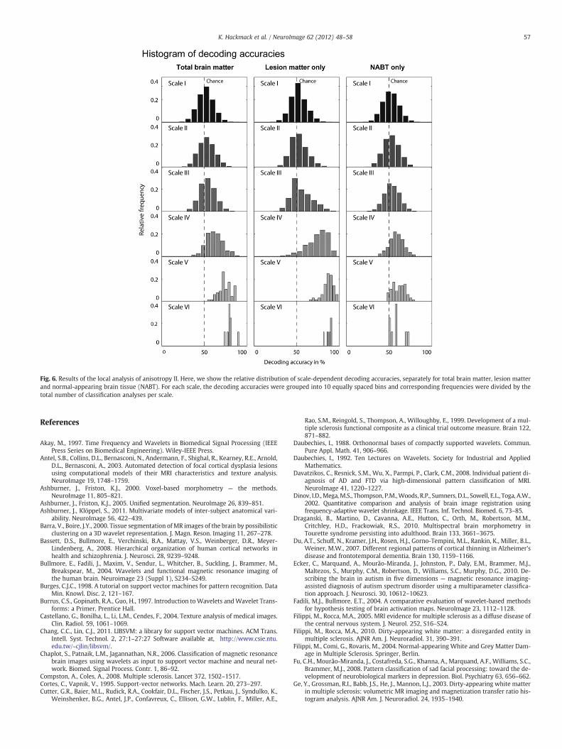
Fig. 6. Results of the local analysis of anisotropy II. Here, we show the relative distribution of scale-dependent decoding accuracies, separately for total brain matter, lesion matterand normal-appearing brain tissue (NABT). For each scale, the decoding accuracies were grouped into 10 equally spaced bins and corresponding frequencies were divided by thetotal number of classification analyses per scale.
57K. Hackmack et al. / NeuroImage 62 (2012) 48–58
References
Akay, M., 1997. Time Frequency and Wavelets in Biomedical Signal Processing (IEEEPress Series on Biomedical Engineering). Wiley-IEEE Press.
Antel, S.B., Collins, D.L., Bernasconi, N., Andermann, F., Shighal, R., Kearney, R.E., Arnold,D.L., Bernasconi, A., 2003. Automated detection of focal cortical dysplasia lesionsusing computational models of their MRI characteristics and texture analysis.NeuroImage 19, 1748–1759.
Ashburner, J., Friston, K.J., 2000. Voxel-based morphometry — the methods.NeuroImage 11, 805–821.
Ashburner, J., Friston, K.J., 2005. Unified segmentation. NeuroImage 26, 839–851.Ashburner, J., Klöppel, S., 2011. Multivariate models of inter-subject anatomical vari-
ability. NeuroImage 56, 422–439.Barra, V., Boire, J.Y., 2000. Tissue segmentation of MR images of the brain by possibilistic
clustering on a 3D wavelet representation. J. Magn. Reson. Imaging 11, 267–278.Bassett, D.S., Bullmore, E., Verchinski, B.A., Mattay, V.S., Weinberger, D.R., Meyer-
Lindenberg, A., 2008. Hierarchical organization of human cortical networks inhealth and schizophrenia. J. Neurosci. 28, 9239–9248.
Bullmore, E., Fadili, J., Maxim, V., Sendur, L., Whitcher, B., Suckling, J., Brammer, M.,Breakspear, M., 2004. Wavelets and functional magnetic resonance imaging ofthe human brain. Neuroimage 23 (Suppl 1), S234–S249.
Burges, C.J.C., 1998. A tutorial on support vector machines for pattern recognition. DataMin. Knowl. Disc. 2, 121–167.
Burrus, C.S., Gopinath, R.A., Guo, H., 1997. Introduction toWavelets andWavelet Trans-forms: a Primer. Prentice Hall.
Castellano, G., Bonilha, L., Li, L.M., Cendes, F., 2004. Texture analysis of medical images.Clin. Radiol. 59, 1061–1069.
Chang, C.C., Lin, C.J., 2011. LIBSVM: a library for support vector machines. ACM Trans.Intell. Syst. Technol. 2, 27:1–27:27 Software available at, http://www.csie.ntu.edu.tw/~cjlin/libsvm/.
Chaplot, S., Patnaik, L.M., Jagannathan, N.R., 2006. Classification of magnetic resonancebrain images using wavelets as input to support vector machine and neural net-work. Biomed. Signal Process. Contr. 1, 86–92.
Compston, A., Coles, A., 2008. Multiple sclerosis. Lancet 372, 1502–1517.Cortes, C., Vapnik, V., 1995. Support-vector networks. Mach. Learn. 20, 273–297.Cutter, G.R., Baier, M.L., Rudick, R.A., Cookfair, D.L., Fischer, J.S., Petkau, J., Syndulko, K.,
Weinshenker, B.G., Antel, J.P., Confavreux, C., Ellison, G.W., Lublin, F., Miller, A.E.,
Rao, S.M., Reingold, S., Thompson, A., Willoughby, E., 1999. Development of a mul-tiple sclerosis functional composite as a clinical trial outcome measure. Brain 122,871–882.
Daubechies, I., 1988. Orthonormal bases of compactly supported wavelets. Commun.Pure Appl. Math. 41, 906–966.
Daubechies, I., 1992. Ten Lectures on Wavelets. Society for Industrial and AppliedMathematics.
Davatzikos, C., Resnick, S.M., Wu, X., Parmpi, P., Clark, C.M., 2008. Individual patient di-agnosis of AD and FTD via high-dimensional pattern classification of MRI.NeuroImage 41, 1220–1227.
Dinov, I.D.,Mega,M.S., Thompson, P.M.,Woods, R.P., Sumners, D.L., Sowell, E.L., Toga, A.W.,2002. Quantitative comparison and analysis of brain image registration usingfrequency-adaptive wavelet shrinkage. IEEE Trans. Inf. Technol. Biomed. 6, 73–85.
Draganski, B., Martino, D., Cavanna, A.E., Hutton, C., Orth, M., Robertson, M.M.,Critchley, H.D., Frackowiak, R.S., 2010. Multispectral brain morphometry inTourette syndrome persisting into adulthood. Brain 133, 3661–3675.
Du, A.T., Schuff, N., Kramer, J.H., Rosen, H.J., Gorno-Tempini, M.L., Rankin, K., Miller, B.L.,Weiner, M.W., 2007. Different regional patterns of cortical thinning in Alzheimer'sdisease and frontotemporal dementia. Brain 130, 1159–1166.
Ecker, C., Marquand, A., Mourão-Miranda, J., Johnston, P., Daly, E.M., Brammer, M.J.,Maltezos, S., Murphy, C.M., Robertson, D., Williams, S.C., Murphy, D.G., 2010. De-scribing the brain in autism in five dimensions — magnetic resonance imaging-assisted diagnosis of autism spectrum disorder using a multiparameter classifica-tion approach. J. Neurosci. 30, 10612–10623.
Fadili, M.J., Bullmore, E.T., 2004. A comparative evaluation of wavelet-based methodsfor hypothesis testing of brain activation maps. NeuroImage 23, 1112–1128.
Filippi, M., Rocca, M.A., 2005. MRI evidence for multiple sclerosis as a diffuse disease ofthe central nervous system. J. Neurol. 252, S16–S24.
Filippi, M., Rocca, M.A., 2010. Dirty-appearing white matter: a disregarded entity inmultiple sclerosis. AJNR Am. J. Neuroradiol. 31, 390–391.
Filippi, M., Comi, G., Rovaris, M., 2004. Normal-appearing White and Grey Matter Dam-age in Multiple Sclerosis. Springer, Berlin.
Fu, C.H., Mourão-Miranda, J., Costafreda, S.G., Khanna, A., Marquand, A.F., Williams, S.C.,Brammer, M.J., 2008. Pattern classification of sad facial processing: toward the de-velopment of neurobiological markers in depression. Biol. Psychiatry 63, 656–662.
Ge, Y., Grossman, R.I., Babb, J.S., He, J., Mannon, L.J., 2003. Dirty-appearing white matterin multiple sclerosis: volumetric MR imaging and magnetization transfer ratio his-togram analysis. AJNR Am. J. Neuroradiol. 24, 1935–1940.

58 K. Hackmack et al. / NeuroImage 62 (2012) 48–58
Graps, A., 1995. An introduction to wavelets. Comput. Sci. Eng. 2, 50–61.Hackmack, K., Weygandt, M., Wuerfel, J., Pfueller, C.F., Bellmann-Strobl, J., Paul, F.,
Haynes, J.D., 2012. Can we overcome the clinico-radiological paradox in multiplesclerosis? J. Neurol. Mar 24 (Electronic publication ahead of print).
Harrison, L.C., Raunio, M., Holli, K.K., Luukkaala, T., Savio, S., Elovaara, I., Soimakallio, S.,Eskola, H.J., Dastidar, P., 2010. MRI texture analysis in multiple sclerosis: toward aclinical analysis protocol. Acad. Radiol. 17, 696–707.
Haynes, J.D., Rees, G., 2006. Decoding mental states from brain activity in humans. Nat.Rev. Neurosci. 7, 523–534.
Haynes, J.D., Sakai, K., Rees, G., Gilbert, S., Frith, C., Passingham, R.E., 2007. Reading hid-den intentions in the human brain. Curr. Biol. 17, 323–328.
He, Y., Chen, Z., Evans, A., 2008. Structural insights into aberrant topological patterns oflarge-scale cortical networks in Alzheimer's disease. J. Neurosci. 28, 4756–4766.
Jafari-Khouzani, K., Elisevich, K., Patel, S., Smith, B., Soltanian-Zadeh, H., 2010. FLAIRsignal and texture analysis for lateralizing mesial temporal lobe epilepsy.NeuroImage 49, 1559–1571.
Kassner, A., Thornhill, R.E., 2010. Texture analysis: a review of neurologic MR imagingapplications. AJNR 31, 809–816.
Kingsbury, N.G., 2000. A dual-tree complex wavelet transform with improved orthog-onality and symmetry properties. Proc. IEEE Int. Conf. Image Proc, Canada, 2, pp.375–378.
Kingsbury, N.G., 2001. Complex wavelets for shift invariant analysis and filtering of sig-nals. Appl. Comput. Harmon. Anal. 10, 234–253.
Klöppel, S., Stonnington, C.M., Barnes, J., Chen, F., Chu, C., Good, C.D., Mader, I., Mitchell,L.A., Patel, A.C., Roberts, C.C., Fox, N.C., Jack Jr., C.R., Ashburner, J., Frackowiak, R.S.,2008a. Accuracy of dementia diagnosis: a direct comparison between radiologistsand a computerized method. Brain 131, 2969–2974.
Klöppel, S., Stonnington, C.M., Chu, C., Draganski, B., Scahill, R.I., Rohrer, J.D., Fox, N.C.,Jack Jr., C.R., Ashburner, J., Frackowiak, R.S., 2008b. Automatic classification of MRscans in Alzheimer's disease. Brain 131, 681–689.
Klöppel, S., Chu, C., Tan, G.C., Draganski, B., Johnson, H., Paulsen, J.S., Kienzle, W.,Tabrizi, S.J., Ashburner, J., Frackowiak, R.S., 2009. PREDICT-HD Investigators of theHuntington Study Group. Automatic detection of preclinical neurodegeneration:presymptomatic Huntington disease. Neurology 72, 426–431.
Koutsouleris, N., Meisenzahl, E.M., Davatzikos, C., Bottlender, R., Frodl, T., Scheuerecker,J., Schmitt, G., Zetzsche, T., Decker, P., Reiser, M., Möller, H.J., Gaser, C., 2009. Use ofneuroanatomical pattern classification to identify subjects in at-risk mental statesof psychosis and predict disease transition. Arch. Gen. Psychiatry 66, 700–712.
Kriegeskorte, N., Goebel, R., Bandettini, P., 2006. Information-based functional brainmapping. Proc. Natl. Acad. Sci. U. S. A. 103, 3863–3868.
Kurtzke, J.F., 1983. Rating neurologic impairment in multiple sclerosis: an expandeddisability status scale (EDSS). Neurology 33, 1444–1452.
Laine, A.F., 2000. Wavelets in temporal and spatial processing of biomedical images.Annu. Rev. Biomed. Eng. 2, 511–550.
Lao, Z., Shen, D., Yue, Z., Karaceli, B., Resnick, S.M., Davatzikos, C., 2004. Morphologicalclassification of brains via high-dimensional shape transformations and machinelearning methods. NeuroImage 21, 46–57.
Loizou, C.P., Murray, V., Pattichis, M.S., Seimenis, I., Pantziaris,M., Pattichis, C.S., 2011.Mul-tiscale amplitude-modulation frequency-modulation (AM-FM) texture analysis ofmultiple sclerosis in brain MRI images. IEEE Trans. Inf. Technol. Biomed. 15, 119–129.
Mallat, S.G., 1989. A theory for multiresolution signal decomposition: the wavelet rep-resentation. IEEE Trans. Pattern Anal. Mach. Intell. 11, 674–693.
Mallat, S., 2008. A Wavelet Tour of Signal Processing. Academic Press.Maxim, V., Sendur, L., Faili, J., Suckling, J., Gould, R., Howard, R., Bullmore, E., 2005. Fractional
Gaussian noise, functional MRI and Alzheimer's disease. NeuroImage 25, 141–158.McDonald,W.I., Compston, A., Edan, G., Goodkin, D., Hartung, H.P., Lublin, F.D., McFarland,
H.F., Paty, D.W., Polman, C.H., Reingold, S.C., Sandberg-Wollheim, M., Sibley, W.,Thompson, A., van den Noort, S., Weinshenker, B.Y., Wolinsky, J.S., 2001. Rec-ommendeddiagnostic criteria formultiple sclerosis: guidelines from the InternationalPanel on the diagnosis of multiple sclerosis. Ann. Neurol. 50, 121–127.
Meyer, Y., 1987. Wavelets with Compact Support. Zygmund Lectures, U. Chicago.Morgen, K., Sammer, G., Courtney, S.M., Wolters, T., Melchior, H., Blecker, C.R.,
Oschmann, P., Kaps, M., Vaitl, D., 2007. Distinct mechanisms of altered brain activa-tion in patients with multiple sclerosis. NeuroImage 37, 937–946.
Mur, M., Bandettini, P.A., Kriegeskorte, N., 2009. Revealing representational contentwith pattern-information fMRI — an introductory guide. Soc. Cogn. Affect. Neu-rosci. 4, 101–109.
Neema, M., Stankiewicz, J., Arora, A., Dandamudi, V.S., Batt, C.E., Guss, Z.D., Al-Sabbagh,A., Bakshi, R., 2007. T1- and T2-based MRI measures of diffuse gray matter and
white matter damage in patients with multiple sclerosis. J. Neuroimaging 17,16S–21S.
Nichols, T., Hayasaka, S., 2003. Controlling the familywise error rate in functional neu-roimaging: a comparative review. Stat. Methods Med. Res. 12, 410–446.
Oliveira Jr., P.P., Nitrini, R., Busatto, G., Buchpiguel, C., Sato, J.R., Amaro Jr., E., 2010. Useof SVM methods with surface-based cortical and volumetric subcortical measure-ments to detect Alzheimer's disease. J. Alzheimers Dis. 19, 1263–1272.
Pujol, J., Soriano-Mas, C., Alonso, P., Cardoner, N., Mechón, J.M., Deus, J., Vallejo, J., 2004.Mapping structural brain alterations in obsessive–compulsive disorder. Arch. Gen.Psychiatry 61, 720–730.
Raj, A., Mueller, S.G., Young, K., Laxer, K.D., Weiner, M., 2010. Network-level analysis ofcortical thickness of the epileptic brain. NeuroImage 52, 1302–1313.
Sailer, M., Fischl, B., Salat, D., Tempelmann, C., Schönfeld, M.A., Busa, E., Bodammer, N.,Heinze, H.J., Dale, A., 2003. Focal thinning of the cerebral cortex in multiple sclero-sis. Brain 126, 1734–1744.
Sajda, P., Lane, A., Zeevi, Y., 2002. Multi-resolution and wavelet representations foridentifying signatures of disease. Dis. Markers 18, 339–363.
Sasikala, M., Kumaravel, N., 2008. A wavelet-based optimal texture feature set for clas-sification of brain tumors. J. Med. Eng. Technol. 32, 198–205.
Schölkopf, B., Smola, A.J., 2002. Learning with Kernels. MIT Press.Selesnick, I.W., Baraniuk, R.G., Kingsbury, N.G., 2005. The dual-tree complex wavelet
transform. IEEE Signal Process. Mag. 22, 123–151.Shawe-Taylor, J., Christianini, N., 2000. Support Vector Machines and Other Kernel-
based Learning Methods. Cambridge University Press.Sowell, E.R., Kan, E., Yoshii, J., Thompson, P.M., Bansal, R., Xu, D., Toga, A.W., Peterson,
B.S., 2008. Thinning of sensorimotor cortices in children with Tourette syndrome.Nat. Neurosci. 11, 637–639.
Suckling, J., Long, C., Triantafyollou, C., Brammer, M., Bullmore, E., 2006. Variable preci-sion registration via wavelets: optimal spatial scales for inter-subject registrationof functional MRI. NeuroImage 15, 197–208.
Unser, M., Aldroubi, A., 1996. A review of wavelets in biomedical applications. Proc.IEEE 84, 626–638.
Van De Ville, D., Blu, T., Unser, M., 2006. Surfing the brain: an overview of wavelet-based techniques for fMRI data analysis. IEEE Eng. Med. Biol. Mag. 25, 65–78.
Vrenken, H., Seewann, A., Knol, D.L., Polman, C.H., Barkhof, F., Geurts, J.J., 2010. Diffuse-ly abnormal white matter in progressive multiple sclerosis: in vivo quantitativeMR imaging characterization and comparison between disease types. AJNR Am. J.Neuroradiol. 31, 541–548.
Weygandt, M., Hackmack, K., Pfüller, C., Bellmann-Strobl, J., Paul, F., Zipp, F., Haynes,J.D., 2011. MRI pattern recognition in multiple sclerosis normal-appearing brainareas. PLoS One 6, e21138.
Worbe, Y., Gerardin, E., Hartmann, A., Valabrégue, R., Chupin, M., Tremblay, L.,Vidailhet, M., Colliot, O., Lehéricy, S., 2010. Distinct structural changes underpinclinical phenotypes in patients with Gilles de la Tourette syndrome. Brain 133,3649–3660.
Yotter, R.A., Nenadic, I., Ziegler, G., Thompson, P.M., Gaser, C., 2011. Local cortical sur-face complexity maps from spherical harmonic reconstructions. NeuroImage 56,961–973.
Zhang, Y., Wells, J., Buist, R., et al., 2006. A novel MRI texture analysis of demyelinationand inflammation in relapsing-remitting experimental allergic encephalomyelitis.Med. Image Comput. Comput. Assist. Interv. 9, 760–767.
Zhang, J., Tong, L., Wang, L., Li, N., 2008. Texture analysis of multiple sclerosis: a com-parative study. Magn. Reson. Imaging 26, 1160–1166.
Zhang, Y., Zhu, H., Mitchell, J.R., et al., 2009. T2 MRI texture analysis is a sensitive mea-sure of tissue injury and recovery resulting from acute inflammatory lesions inmultiple sclerosis. NeuroImage 47, 107–111.
W E B R E F E R E N C E S
SPM5 software (Wellcome Trust Centre for Neuroimaging, Institute of Neurology,UCL, London): http://www.fil.ion.ucl.ac.uk/spm; last time accessed: November4th 2011.
Wavelet software (Electrical and Computer Engineering Polytechnic University, NewYork): http://taco.poly.edu/WaveletSoftware/; last time accessed: November 4th2011.
LIBSVM software (Department of Computer Science, National Taiwan University,Taiwan):http://www.csie.ntu.edu.tw/~cjlin/libsvm/; last time accessed: Novem-ber 4th 2011.