Embed Size (px)
Citation preview

HAL Id: hal-03236238https://hal.archives-ouvertes.fr/hal-03236238v3
Submitted on 17 Nov 2021
HAL is a multi-disciplinary open accessarchive for the deposit and dissemination of sci-entific research documents, whether they are pub-lished or not. The documents may come fromteaching and research institutions in France orabroad, or from public or private research centers.
L’archive ouverte pluridisciplinaire HAL, estdestinée au dépôt et à la diffusion de documentsscientifiques de niveau recherche, publiés ou non,émanant des établissements d’enseignement et derecherche français ou étrangers, des laboratoirespublics ou privés.
Multi-stage Stochastic Alternating Current OptimalPower Flow with Storage: Bounding the Relaxation Gap
Maxime Grangereau, Wim van Ackooij, Stéphane Gaubert
To cite this version:Maxime Grangereau, Wim van Ackooij, Stéphane Gaubert. Multi-stage Stochastic Alternating Cur-rent Optimal Power Flow with Storage: Bounding the Relaxation Gap. Electric Power SystemsResearch, Elsevier, 2022, 206, pp.107774. 10.1016/j.epsr.2022.107774. hal-03236238v3

Multi-stage Stochastic Alternating Current Optimal Power
Flow with Storage: Bounding the Relaxation Gap
Maxime Grangereaua,b,∗, Wim van Ackooijb, Stephane Gauberta,c
aEcole polytechnique, IP Paris, CMAP, CNRS, Route de Saclay, 91300 PalaiseaubEDF Lab Saclay, Route de Saclay 91300 PalaiseaucINRIA Saclay, Route de Saclay, 91300 Palaiseau
Abstract
We propose a generic multistage stochastic model for the Alternating Current Optimal
Power Flow (AC OPF) problem for radial distribution networks, to account for the
random electricity production of renewable energy sources and dynamic constraints of
storage systems. We consider single-phase radial networks. Radial three-phase balanced
networks (medium-voltage distribution networks typically have this structure) reduce
to the former case. This induces a large scale optimization problem, which, given the
non-convex nature of the AC OPF, is generally challenging to solve to global optimality.
We derive a priori conditions guaranteeing a vanishing relaxation gap for the multi-stage
AC OPF problem, which can thus be solved using convex optimization algorithms. We
also give an a posteriori upper bound on the relaxation gap. In particular, we show that
a null or low relaxation gap may be expected for applications with light reverse power
flows or if sufficient storage capacities with low cost are available. Then, we discuss
the validity of our results when incorporating voltage regulation devices. Finally, we
illustrate our results on problems of planning of a realistic distribution feeder with
distributed solar production and storage systems. Scenario trees for solar production
∗Corresponding authorEmail addresses: [email protected]; [email protected];
[email protected] (Maxime Grangereau), [email protected] (Wimvan Ackooij), [email protected] (Stephane Gaubert)
Preprint submitted to Electric Power Systems Research November 17, 2021
are constructed from a stochastic model, by a quantile-based algorithm.
Keywords: Optimal Power Flow, multistage stochastic optimization, convex
relaxation, second-order cone programming, scenario trees
1. Introduction
1.1. Motivation
Distribution networks are currently facing a major change owing to the increasing
share of decentralized Renewable Energy Sources (RES). They can create local physi-
cal violations and induce uncertainty on the network operating point: their production
levels are random, as a result of the weather. To cope with these issues, many Distri-
bution Network Operators (DNOs) are required to become able to respond locally to
unforeseen events. This can be done by the means of energy flexibilities located at the
nodes of the network, like storage systems. The dynamical and sometimes uncertain
nature of these subsystems as well as the uncertainty brought by RES should be taken
into account in the operation planning tools used by DNOs. One of these relevant tools
is the so-called Optimal Power Flow (OPF) problem. It is a mathematical optimization
problem which aims at finding an operating point of a power network that minimizes
a given objective function, such as generation costs, active power losses, subject to
constraints on power injections and losses, voltage magnitudes and intensities in the
lines. We are interested in the Alternating Current Optimal Power Flow (AC OPF)
problem which is an accurate physical model of the operating point of a network. It
is non-convex and traditionally used in a static deterministic framework. However, as
argued before, a stochastic and dynamic framework with storage systems and RES is
of practical interest and this is the focus of the present paper.
2

1.2. Optimal Power Flow Problem
There exist two main declinations of the AC OPF problem: the Bus Injection Model
(BIM), and the Branch Flow Model (BFM), both presented in [1]. Both formulations
are equivalent for radial connected networks [2]. In this paper, we choose the BFM
formulation since it makes our arguments easier to present. The AC OPF problem is a
non-convex optimization problem, recently shown to be strongly NP-hard [3]. However,
a series of recent works initiated by the seminal paper [4] have shown that many real-
world instances can be solved to global optimality using convex relaxations of the
original problem.
A very extensive overview on relaxations and approximations of AC Power flow equa-
tions can be found in the book [5], while a particular focus on conic relaxations is given
in [6]. We focus here on results on the conic relaxations of AC OPF problems for single
phase radial networks. These models allow to treat the case of balanced three-phase
radial networks, like medium voltage distribution networks (20 kV) in France, which
reduces to the former case. The most famous conic relaxations of the AC OPF Problem
are the Second-Order Cone (SOC) relaxation and the Semi-Definite (SD) relaxation.
Both are presented in details in [1]. For radial networks, the SOC and SD relaxations
are equivalent, but the SOC relaxation exhibits better numerical performance, and is
preferable for such topologies. Conic relaxations are often used in the literature owing
to their enhanced numerical performance and for the certificate of optimality they may
provide, compared with the non-convex formulation. They are exact for many practical
instances of OPF problem [4]. For this reason, many authors have studied exactness
conditions for these convex relaxations. A posteriori conditions on the solution of the
dual problem are given in [4]. The relaxation is exact for radial connected network un-
der assumptions like over-generation [7], load over-satisfaction [8], or no upper bounds
on voltage magnitude [9]. As these conditions are not verified by practical instances,
3

other authors [10, 11] have obtained more realistic a priori exactness conditions.
1.3. Contributions
In this paper, we develop a generic model for the multi-stage stochastic version
of the AC Optimal Power Flow problem with storage systems and intermittent RES.
Multistage stochastic models allow to ensure the non-anticipativity of decision variables
and are a pre-requisite in order to prevent decisions to depend on the realization of yet
unknown data. These models require the formulation of a scenario tree, the size of
which, has to grow exponentially with the number of time stages [12]. The multistage
stochastic AC OPF problem is therefore a non-convex and large-scale problem. To
alleviate the non-convexity issue, we consider the SOC relaxation of the problem. Our
main contribution is to show that approaches guaranteeing the absence of relaxation
gap for the AC OPF problem, originally developed in a static deterministic setting,
can be extended to the multi-stage stochastic setting. Inspired by the approach of
[11] in the deterministic case, we propose to restrict the feasible set of the problem by
adding a finite number of linear constraints, which impose feasibility of a linearized
power flow and compensations for active or reactive reverse power flows in the network.
We show that the restricted problem has the same optimal value as the original one
under realistic assumptions which can easily be checked a priori, see Proposition 1.
The restricted problem has no relaxation gap, and hence its optimal value is easily
computable, see Theorem 1. This allows us to easily compute a feasible solution of the
original problem and an a posteriori upper bound on its relaxation gap, see Theorem
2. Besides, the result provides realistic and tractable a priori conditions guaranteeing
that the relaxation gap of the original problem is zero, see Theorem 3. Validity of
our result when considering voltage regulation devices such as uncontrollable Voltage
Regulation Transformers, SVCs and STATCOMs is also shown. The interest of our
results is numerically illustrated on a realistic distribution network with 56 buses found
4

in [13], equipped with distributed storage and solar panels. We generate the scenario
trees for solar production by a quantile-based algorithm, based on a stochastic model
of solar irradiance.
1.4. Related work
By comparison with other works guaranteeing zero relaxation gap for the AC OPF
problem [4, 7, 8, 9, 10, 11], we consider a multistage stochastic setting. The conditions
given in our paper extend to the multistage stochastic case and to more general cost
functionals the realistic zero relaxation gap conditions given in [11]. Moreover, we use
this approach to provide a posteriori bounds on the relaxation gap.
Several works consider a deterministic dynamic AC OPF model, like [14], which
considers the SOC relaxation.
Some recent research proposes probabilistic (indifferently called chance-constrained)
versions of the OPF problem. A probabilistic AC OPF model linearized around a refer-
ence scenario is studied in [15]. Other works consider the robust counterpart of the SD
relaxation restricted to affine-linear decision-rules [16]. A Semi-Definite convex relax-
ation of the chance-constrained AC OPF problem is proposed in [17] using a scenario
based-approach and assuming piece-wise linear decision rules, or assuming Gaussian
uncertainty. A Second-Order Cone approximation of the chance-constrained AC OPF
is proposed in [18] which allows good numerical performances, combined with a feasi-
bility recovery method. None of these references account for storage systems, nor do
they consider dynamical aspects of the problem.
Several other works deal with dynamic stochastic models. In particular, an impor-
tant requirement for such problems is to ensure that decision variables remain non-
anticipative, i.e., do not depend on yet unobserved random data. References [19] con-
siders the simplified case where decision are non-anticipative for the initial time steps
only. Non-anticipativity is guaranteed in [20] using affine-linear policies but with a
5

(linear) DC OPF model. Non-anticipativity of the decisions is also guaranteed in [21]
which considers an iterative procedure to optimize a decision policy. By comparison,
the approach by scenario trees developed here accounts both for non-anticipativity con-
straints and for the nonlinearity of the stochastic OPF problem, whereas it benefits from
theoretical convergence guarantees. Indeed, scenario tree methods provide an approxi-
mation of the value of the original problem with continuous distribution of the random
data, and this approximation converges to this value when the number of scenarios goes
to infinity [12].
1.5. Outline of the paper
This paper is organized as follows. Section 2 presents the multi-stage stochastic AC
OPF problem. Section 3 introduces a restriction of this problem and gives conditions
ensuring equality of the values of the original and restricted problems. Section 4 presents
the main result of this paper: the restricted problem has no relaxation gap. This
provides a convenient way to establish a priori exactness of the SOC relaxation for
particular instances of the original problem, or an easily computable bound on the
relaxation gap. Section 5 discusses validity and possible extensions of our result when
incorporating voltage regulation devices or when considering multi-phase unbalanced
networks. We illustrate numerically our results on a realistic distribution networks with
56 buses in Section 6.
1.6. Notation
The set of real numbers is denoted by R and the set of complex numbers by C. The
notation i stands for the purely imaginary number such that i2 = −1. For z ∈ C, <(z)
stands for its real part, =(z) for its imaginary part, z∗ for its complex conjugate and
|z| for its modulus. The set of time steps is denoted by T , the set of buses by B, the
set of edges by E (directed towards the root of the tree for acyclic networks), the set
6

of scenarios by Ω. The impedance of an edge−−→(i, j) ∈ E is denoted by zi,j ∈ C, with
resistance ri,j := <(zi,j), and reactance xi,j := =(zi,j). We denote vectors indexed by a
set I according to a := (ai)i∈I .
2. The multistage stochastic AC OPF model
2.1. Formulation of the problem
Throughout the work, we will make the assumption that the network is radial,
connected and passive, i.e., <(zi,j) ≥ 0 and =(zi,j) ≥ 0 for all lines−−→(i, j) ∈ E of the
network. We formulate a multi-stage stochastic AC OPF problem with a battery storage
system at each bus of the network (except for the reference bus 0) using the Branch
Flow Model, presented in [1, 13], which we extend to the multi-stage stochastic case.
We next describe the multistage stochastic AC OPF problem in Branch Flow Model
formulation. We impose the following constraints. First, we consider the constraints
on voltage squared magnitudes v:
v0,t,ω = 1, t ∈ T , ω ∈ Ω, (1)
vi ≤ vi,t,ω ≤ vi, i ∈ B \ 0, t ∈ T , ω ∈ Ω. (2)
We also incorporate bounds on intensity squared magnitude I:
0 ≤ I−−→(i,j),t,ω
≤ I−−→(i,j)
,−−→(i, j) ∈ E , t ∈ T , ω ∈ Ω. (3)
We consider bounds on sending-end power flow S magnitudes in the lines of the network,
which is a convex quadratic constraint:
∣∣∣S−−→(i,j),t,ω
∣∣∣ ≤ S−−→(i,j)
,−−→(i, j) ∈ E , t ∈ T , ω ∈ Ω. (4)
7
We consider bound constraints on active power injected pinj, absorbed pabs by batteries
and flexible reactive power injected q (which can account for SVCs and STATCOMs,
[22]):
0 ≤ pinji,t,ω ≤ pinj
i , i ∈ B \ 0, t ∈ T , ω ∈ Ω, (5)
0 ≤ pabsi,t,ω ≤ pabs
i , i ∈ B \ 0, t ∈ T , ω ∈ Ω, (6)
qi≤ qi,t,ω ≤ qi, i ∈ B \ 0, t ∈ T , ω ∈ Ω. (7)
We introduce the constraints on the states of charge of the batteries X, which represent
respectively their dynamics (accounting for different efficiencies when charging and
discharging the batteries), their initial values and their physical bounds for all i ∈
B \ 0, ω ∈ Ω, denoting ∆t the time duration of step t ∈ T :
Xi,t+1,ω = Xi,t,ω + ρabsi pabs
i,t,ω∆t − ρinji p
inji,t,ω∆t, t ∈ T \ T, (8)
Xi,0,ω = xi, (9)
X i ≤ Xi,t,ω ≤ X i, t ∈ T . (10)
Then we consider the expression of the complex power injections s at all buses of the
network i ∈ B \ 0, for all time steps t ∈ T and scenario ω ∈ Ω:
si,t,ω = pinji,t,ω − pabs
i,t,ω + iqi,t,ω − sdi,t,ω. (11)
8

This allows to formulate the power balance equations at the non-slack buses and the
slack bus 0, for all−−→(i, j) ∈ E , t ∈ T , ω ∈ Ω:
S−−→(i,j),t,ω
=∑−−→(k,i)∈E
(S−−→(k,i),t,ω
− zk,iI−−→(k,i),t,ω) + si,t,ω, (12)
0 =∑−−→(k,0)∈E
(S−−→(k,0),t,ω
− zk,0I−−→(k,0),t,ω) + s0,t,ω. (13)
We consider also the voltage propagation constraint and the constraint making the link
between voltage squared magnitudes v, intensity squared magnitudes I and sending-end
power flows S in the network, for all−−→(i, j) ∈ E , t ∈ T , ω ∈ Ω:
vi,t,ω − vj,t,ω = 2<(z∗i,jS−−→(i,j),t,ω)− |zi,j|2I−−→(i,j),t,ω
, (14)
vi,t,ωI−−→(i,j),t,ω= |S−−→
(i,j),t,ω|2. (15)
Constraint (15) is a non-convex quadratic equality constraint. Last, we consider the
non-anticipativity constraint, which encodes the fact that decision variables y should
not depend on yet unknown realization of random data of the problem:
y is non anticipative. (16)
More details shall be given later on the formulation of the non-anticipativity constraints.
We consider a general (possibly random, progressively-measurable) convex cost function
C depending on all decision variables of the problem. We can now formulate the multi-
9
stage stochastic AC-OPF problem:
miny=(s0,s,pinj,pabs,q,X,S,I,v)
E[C(s0, p
inj, pabs, q, S, I, X)]
s.t. (1)− (16).
We denote this optimization problem by (P ). It is a non-convex problem owing to
Constraint (15). Decision variables are listed and described in Table 1.
Decision variable Descriptions0 = (s0,t,ω)t∈T ,ω∈Ω Apparent power injections at bus 0s = (si,t,ω)i∈B,t∈T ,ω Apparent power injections
pinj = (pinji,t,ω)i∈B,t∈T ,ω Injected active power by storage systems
pabs = (pabsi,t,ω)i∈B,t∈T ,ω Absorbed active power by storage systems
q = (qi,t,ω)i∈B,t∈T ,ω Injected reactive power by flexible systemsS = (S−−→
(i,j),t,ω)−−→(i,j)∈E,t∈T ,ω∈Ω
Apparent power in lines
I = (I−−→(i,j),t,ω
)−−→(i,j)∈E,t∈T ,ω∈Ω
Squared magnitudes of intensities
v = (vi,t,ω)i∈B,t∈T ,ω Squared magnitudes of voltages
Table 1: Decision variables
2.2. On the formulation of the non-anticipativity constraints
We define a scenario tree, which allows to formulate a problem with a finite number
of scenarios while accounting for the filtration structure. Each scenario ω ∈ Ω is
associated with a trajectory ξω = (ξt,ω)t∈T of the exogenous random process impacting
the system and can be visualized as a path from the root to the leaves of the scenario
tree. Scenarios ω and ω′ are said to be indistinguishable up to time t if ξτ,ω = ξτ,ω′ for
any τ ≤ t. If x = (xt,ω)t∈T ,ω∈Ω denotes the decision variable of a multi-stage stochastic
problem, and xt,ω denotes the decision taken at time t for scenario ω, non-anticipativity
can be expressed by the following constraint for all time t ∈ T and all scenarios ω
and ω′ indistinguishable up to time t: xt,ω = xt,ω′ . Good scenario trees should grow
exponentially fast with the number of time stages [12] to appropriately approximate
10

the distribution and the filtration generated by the random noise.
2.3. Second-Order Cone relaxation of the problem
As we already observed, constraint (15) is non-convex. Relaxing it into an inequality
constraint:
vi,t,ωI−−→(i,j),t,ω≥ |S−−→
(i,j),t,ω|2,
−−→(i, j) ∈ E , t ∈ T , ω ∈ Ω, (17)
yields a convex problem, denoted (PSOC). This problem is called the Second-Order
Cone Relaxation of the problem, and is given by:
miny=(s0,s,pinj,pabs,q,X,S,I,v)
E[C(s0, p
inj, pabs, q, S, I, X)]
s.t. (1)− (14), (16), (17).
Indeed, (17) has the structure of a rotated second-order cone constraint x1x2 ≥
x23 + x2
4.
3. Restriction of the feasible set
3.1. Presentation of the problem with restricted feasible set
We present a variant of Problems (P ) and (PSOC), obtained by adding a finite num-
ber of linear inequalities. Consider additional variables vLin = (vLini,t,ω)i∈B,t∈T ,ω∈Ω, which
plays the role of the square voltage magnitude variable, SLin = (SLin−−→(i,j),t,ω
)−−→(i,j)∈E,t∈T ,ω∈Ω
,
which plays the role of the sending-end power flow variable, and sLin0 = (sLin
0,t,ω)t∈T ,ω∈Ω,
which plays the role of the power injections at the slack bus 0. We first consider the
11
constraints of the Linearized DistFlow model [23]:
vLin0,t,ω = 1, t ∈ T , ω ∈ Ω, (18)
vLini,t,ω ≤ vi, i ∈ B, t ∈ T , ω ∈ Ω, (19)
SLin−−→(i,j),t,ω
=∑−−→(k,i)∈E
SLin−−→(k,i),t,ω
+ si,t,ω,−−→(i, j) ∈ E , t ∈ T , ω ∈ Ω, (20)
0 =∑−−→(k,0)∈E
SLin−−→(k,0),t,ω
+ sLin0,t,ω, t ∈ T , ω ∈ Ω, (21)
vLini,t,ω − vLin
j,t,ω = 2<(z∗i,jSLin−−→(i,j),t,ω
),−−→(i, j) ∈ E , t ∈ T , ω ∈ Ω. (22)
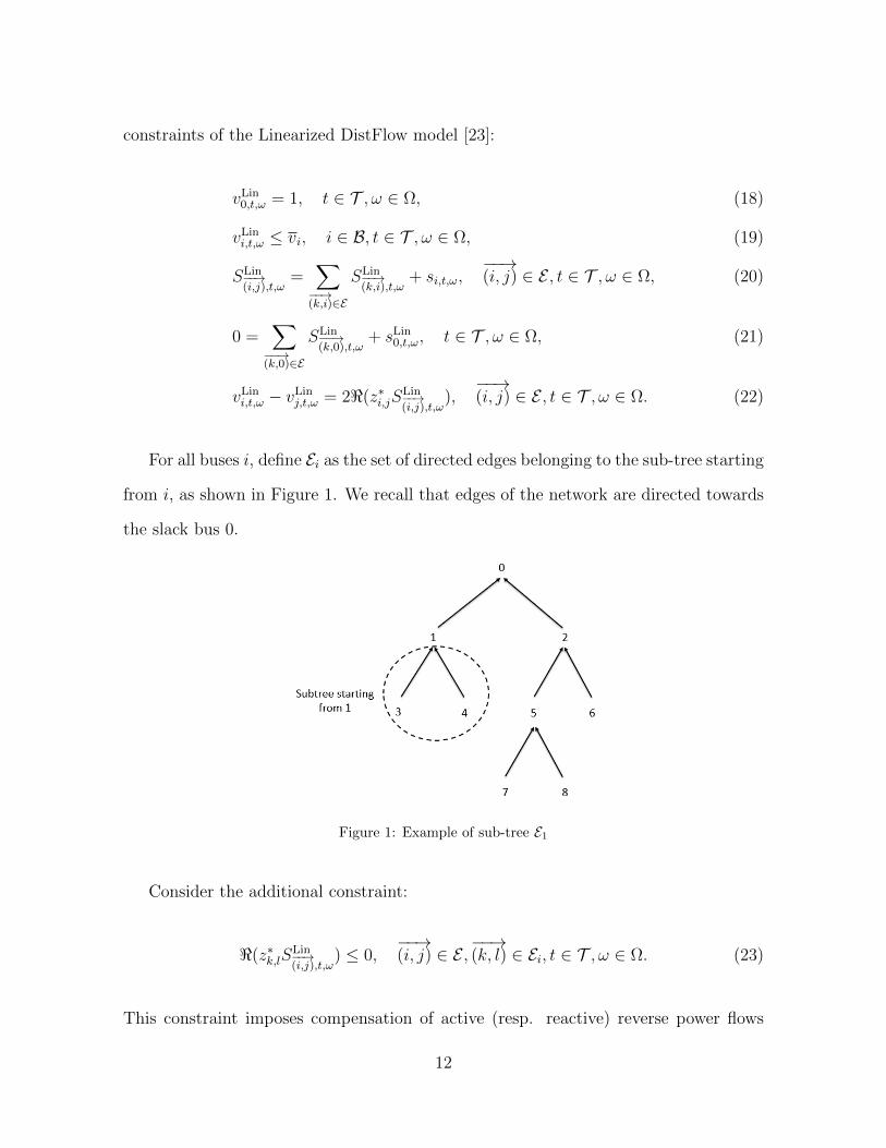
For all buses i, define Ei as the set of directed edges belonging to the sub-tree starting
from i, as shown in Figure 1. We recall that edges of the network are directed towards
the slack bus 0.
Figure 1: Example of sub-tree E1
Consider the additional constraint:
<(z∗k,lSLin−−→(i,j),t,ω
) ≤ 0,−−→(i, j) ∈ E ,
−−→(k, l) ∈ Ei, t ∈ T , ω ∈ Ω. (23)
This constraint imposes compensation of active (resp. reactive) reverse power flows
12

in the lines of the network by forward reactive (resp. active) power flow along the
same lines. Denoting y := (s0, s, pinj, pabs, q,X, S, I, v, SLin, vLin, sLin
0 ) as the vector of
all decision variables, we can now introduce the problem (P ′):
miny
E[C(s0, p
inj, pabs, q, S, I, X)]
s.t. (1)− (16), (18)− (23).
In particular, the value of (P ′) is an upper bound on the value of (P ): val(P ) ≤ val(P ′).
3.2. Second-order cone relaxation of the problem with restricted feasible set
Similarly as before, we can introduce the second-order cone relaxation of the new
problem (P ′) by replacing the non-convex quadratic equality constraints (15) by the
rotated second-order cone constraints (17). This convex relaxation is denoted (P ′SOC)
and can be efficiently solved.
3.3. Conditions ensuring equality of the feasible sets of the original and restricted prob-
lems
We show that, under realistic and easily verifiable a priori conditions, the feasible
sets of (P ′) and (P ) coincide. Denote si,t,ω = pinji + iqi − sdi,t,ω an upper bound on
total power injections at bus i at time step t for scenario ω, obtained for instance using
Constraints (5), (6), (7) and (11). For ω ∈ Ω, t ∈ T , define vLin = (vLint,ω )t∈T ,ω∈Ω and
SLin = (SLint,ω )t∈T ,ω∈Ω by:
SLin−−→
(i,j),t,ω=∑−−→(k,i)∈E S
Lin−−→(k,i),t,ω
+ si,t,ω,−−→(i, j) ∈ E ,
vLin0,t,ω = 1,
vLini,t,ω − vLin
j,t,ω = 2<(z∗i,jSLin−−→(i,j),t,ω
),−−→(i, j) ∈ E .
(24)
13

Proposition 1. Define (vLin, SLin) as the unique solution of the system (24). Assume
the network is radial, connected and passive (i.e., for all lines−−→(i, j) ∈ E, it holds that
zi,j ≥C 0) and moreover:
vLini,t,ω ≤ vi, i ∈ B, t ∈ T , ω ∈ Ω,
<(z∗k,lSLin−−→(i,j),t,ω
) ≤ 0,−−→(i, j) ∈ E ,
−−→(k, l) ∈ Ei, t ∈ T , ω ∈ Ω.
(25)
For any feasible point y of (P ) (resp. (PSOC)), define (sLin0 , vLin, SLin) as the unique solu-
tion of the linear system defined by (18)-(20)-(21)-(22). Then y′ := (y, sLin0 , vLin, SLin)
is feasible with respect to (P ′) (resp. (P ′SOC)). In particular, val(P ) = val(P ′) and
val(PSOC) = val(P ′SOC).
Proof. Consider a feasible point y := (s, v, S, I) of (P ) (resp. (PSOC)). Then, we have
si,t,ω ≤C si,t,ω for all i ∈ B \ 0, t ∈ T , ω ∈ Ω. Define (sLin0 , vLin, SLin) by (18)-(20)-
(21)-(22). In particular, we have:
SLin−−→(i,j),t,ω
≤C SLin−−→(i,j),t,ω
−−→(i, j) ∈ E , t ∈ T , ω ∈ Ω.
Using the above, the assumption of a passive network and (25), we have:
<(z∗k,lSLin−−→(i,j),t,ω
) ≤ <(z∗k,lSLin−−→(i,j),t,ω
) ≤ 0,−−→(i, j) ∈ E ,
−−→(k, l) ∈ Ei, t ∈ T , ω ∈ Ω,
which shows that (23) holds. We also get for all−−→(i, j) ∈ E , t ∈ T , ω ∈ Ω:
vLini,t,ω − vLin
j,t,ω = 2<(z∗i,jSLin−−→(i,j),t,ω
) ≤ 2<(z∗i,jSLin−−→(i,j),t,ω
) = vLini,t,ω − vLin
j,t,ω ,
which implies vLini,t,ω ≤ vLin
i,t,ω ≤ vi for all i ∈ B, using (1), (18) and the orientations of the
edges towards the slack bus 0. This shows that y′ := (y, sLin0 , vLin, SLin) is feasible for
14

(P ′) (resp (P ′SOC)).
Remark 1. The above Proposition implies condition C1 in [11], which is an abstract
assumption on the feasible set of the problem, but it is easier to check.
The following Proposition shows that if there are no reverse power flows in the
network, (25) holds.
Proposition 2. Define (vLin, SLin) as the unique solution of the system (24). Assume
the network is radial, connected and passive, that vi ≥ 1 for all buses i ∈ B and the
following condition holds:
SLin−−→(i,j),t,ω
≤C 0,−−→(i, j) ∈ E , t ∈ T , ω ∈ Ω. (26)
Then (25) holds.
Proof. Under (26) and the assumption of a passive network, we have:
vLini,t,ω − vLin
j,t,ω = 2<(z∗i,jSLin−−→(i,j),t,ω
) ≤ 0,−−→(i, j) ∈ E , t ∈ T , ω ∈ Ω,
which implies for all i ∈ B, t ∈ T , ω ∈ Ω, vLini,t,ω ≤ vLin
0,t,ω = 1 ≤ vi, using (1), (18) and
the orientations of the edges towards the slack bus 0. One can then easily show that
(25) holds.
Remark 2. Let us notice that condition (26) is verified if:
si,t,ω ≤C 0, i ∈ B \ 0, t ∈ T , ω ∈ Ω. (27)
4. Vanishing relaxation gap for the problem with restricted feasible set
We now prove that the problem with restricted feasible set has no relaxation gap,
i.e., val(P ′SOC) = val(P ′). The proof of this result relies on an appropriate relabeling of
15

the buses, then on an iterative scheme inspired by [11]. By comparison with the latter
reference, we consider a multi-stage stochastic setting (in particular, we show that non-
anticipativity is preserved throughout the iterations) and we allow more general cost
functions. We make the following assumption, which can be ensured by appropriately
re-indexing the buses:
(H.Lab) The buses are labeled in non-decreasing order according to their depths in the
tree, see Figure 1.
The iterative scheme we consider takes as input a feasible point y(0) of (P ′SOC), and
at every iteration, constructs a new feasible point of (P ′SOC) using a Forward-Backward
Sweep method, see Algorithm 1. We shall see that the repeated applications of the
Forward-Backward Sweep method 1 generates a convergent sequence of feasible points
(y(k))k∈N of (P ′SOC), each of them being non-anticipative, and that the limit satisfies the
constraints of the non-convex problem (P ′).
Algorithm 1 Forward-Backward sweep method
1: Inputs: (s0, S, I, v).2: for ω ∈ Ω, t ∈ T do3: for i = n, n− 1, ..., 1 do
4: Let j be the unique node in B such that−−→(i, j) ∈ E with the new labels.
5: S′−−→(i,j),t,ω
← si,t,ω +∑−−→(k,i)∈E(S
′−−→(k,i),t,ω
− zk,iI ′−−→(k,i),t,ω
).
6: I ′−−→(i,j),t,ω
←|S′−−→
(i,j),t,ω|2
vi,t,ω.
7: end for8: s′0,t,ω ← −
∑−−→(k,0)∈E(S
′−−→(k,0),t,ω
− zk,0I ′b,0,t,ω).
9: v′0,t,ω ← 1.10: for i = 1, 2, ..., n do
11: Let j be the unique node in B such that−−→(i, j) ∈ E with the new labels.
12: v′i,t,ω ← v′j,t,ω + 2<(z∗i,jS′−−→(i,j),t,ω
)− |zi,j |2I ′−−→(i,j),t,ω
.
13: end for14: end for
15: Outputs: (s′0, S′, I ′, v′).
16
Lemma 1. Let y := (s0, s, pinj, pabs, X, S, I, v, vLin, SLin, sLin0 ) be a feasible solution of
(P ′SOC), with . Then, if the network is passive (meaning that for all lines−−→(i, j) ∈ E, we
have zi,j ≥C 0), the following inequalities are valid:
S−−→(i,j),t,ω
≤C SLin−−→(i,j),t,ω
, ∀−−→(i, j) ∈ E , t ∈ T , ω ∈ Ω,
s0,t,ω ≥C sLin0,t,ω, ∀t ∈ T , ω ∈ Ω,
vi,t,ω ≤ vLini,t,ω, ∀i ∈ B, t ∈ T , ω ∈ Ω.
Proof. The claimed inequalities are established t by t and ω by ω. We drop the corre-
sponding indices for simplicity of the notations. The inequalities on S and SLin arise
from the constraint (3) which implies that I is non-negative component-wise, from pas-
sivity of the network and from constraints (12) and (20). The inequalities on s0 and
sLin0 can then be deduced by the inequality between S and SLin and constraints (13) and
(21). Comparing (14) and (22), using the passivity of the network and the inequalities
between S and SLin, one gets for all−−→(i, j) in E :
vi − vj ≤ vLini − vLin
j .
We can then show the inequalities on v and vLin using the fact that vLin0 = 1 = v0, by
(1) and (18), and using the fact that edges are directed towards the slack bus (root of
the tree) indexed by 0.
Lemma 2. Algorithm 1 is well-posed. Let y be a feasible solution of (P ′SOC), defined by
y := (s0, s, pinj, pabs, X, S, I, v, vLin, SLin, sLin0 ). Apply Algorithm 1 once to (s0, S, I, v)
17
and denote by (s′0, S′, I ′, v′) its output. Then we have:
S−−→(i,j),t,ω
≤C S′−−→(i,j),t,ω
, ∀−−→(i, j) ∈ E , t ∈ T , ω ∈ Ω,∣∣∣S−−→
(i,j),t,ω
∣∣∣ ≥ ∣∣∣S ′−−→(i,j),t,ω
∣∣∣ , ∀−−→(i, j) ∈ E , t ∈ T , ω ∈ Ω,
I−−→(i,j),t,ω
≥ I ′−−→(i,j),t,ω
, ∀−−→(i, j) ∈ E , t ∈ T , ω ∈ Ω,
s0,t,ω ≥C s′0,t,ω, ∀t ∈ T , ω ∈ Ω,
vi,t,ω ≤ v′i,t,ω, ∀i ∈ B, t ∈ T , ω ∈ Ω.
Moreover, y′ := (s0, s, pinj, pabs, X, S, I, v, vLin, SLin, sLin0 ) is feasible for (P ′SOC). In par-
ticular, it is non-anticipative.
Proof. The claimed inequalities are established t by t and ω by ω. We drop the corre-
sponding indices for simplicity of the notations. The definition of S for leaves of the tree
in the forward pass is well-defined as the sum in the LHS is empty in this case by our
labels (Algorithm 1, line 6). The labels chosen ensure that the forward pass always ex-
plores leaves before their ancestors, which ensures that the forward pass is well-defined.
Therefore, the whole algorithm is well-posed. Consider the forward pass, with i = n, n
being the index of the last bus after setting the new labels (see Assumption (H.Lab)).
Denoting j its unique ancestor, we have S−−−→(n,j)
= sn = S ′−−−→(n,j)
by construction. We then
obtain, using the fact that y satisfies (17):
I ′−−−→(n,j)
= |S ′−−−→(n,j)|2/vn = |S−−−→
(n,j)|2/vn ≤ I−−−→(n,j)
.
Let us now assume i < n, and we assume the inequalities for S, S ′, I and I ′ have
been proved for all k = i+ 1, ..., n. If i is a leaf, we can prove the inequalities similarly
as for i = n. Consider the case where i < n is not a leaf. Let j be its unique ancestor.
18
Then, by passivity of the network:
S ′−−→(i,j)
= si +∑−−→(k,i)∈E
(S ′−−→(k,i)− zk,iI ′−−→
(k,i)) ≥C si +
∑−−→(k,i)∈E
(S−−→(k,i)− zk,iI−−→(k,i)
) = S−−→(i,j)
.
Besides, denoting P := <(S), Q := =(S), P Lin := <(SLin) and QLin := =(SLin):
|S ′−−→(i,j)|2 − |S−−→
(i,j)|2 = (P ′−−→
(i,j)+ P−−→
(i,j))(P ′−−→
(i,j)− P−−→
(i,j)) + (Q′−−→
(i,j)+Q−−→
(i,j))(Q′−−→
(i,j)−Q−−→
(i,j))
≤ 2P Lin−−→(i,j)
(P ′−−→(i,j)− P−−→
(i,j)) + 2QLin−−→
(i,j)(Q′−−→
(i,j)−Q−−→
(i,j))
= −2
∑(k,l)∈Ei
(P Lin−−→(i,j)
rk,l +QLin−−→(i,j)
xk,l)(I ′−−→(k,l)− I−−→
(k,l))
= −2
∑−−→(k,l)∈Ei
<(z∗k,lSLin−−→(i,j)
)(I ′−−→(k,l)− I−−→
(k,l))
≤ 0.
In the inequality in the third line, we used Lemma 1, then we use the definition of S ′
and the fact that S satisfies (12) to obtain the following equality. The last inequality is
obtained using I ′−−→(k,l)≥ I−−→
(k,l)for all
−−→(k, l) ∈ Ei and the fact that SLin satisfies (23). We
then obtain:
I ′−−→(i,j)
= |S ′−−→(i,j)|2/vi ≤ |S−−→(i,j)
|2/vi ≤ I−−→(i,j).
The inequality s0 ≥C s′0 can then be deduced from the first and third above in-
equality and the assumption of passivity of the network. We have v0 = 1 = v′0 by
construction and by (1). Notice then that for all−−→(i, j) ∈ E , by construction of v′ and
by (14):
v′i − vi ≥ v′j − vj,
where we used the earlier inequalities on S, S ′, I and I ′ and the assumption of passivity
19

of the network. By propagating this in the network from 0 to n, we get the desired
inequality on the voltage squared magnitudes. We have:
∀−−→(i, j) ∈ E , I ′−−→
(i,j)= |S ′−−→
(i,j)|2/vi ≥ |S ′−−→
(i,j)|2/v′i.
Hence (S ′, v′, I ′) satisfies (17). Let y′ := (s0, s, pinj, pabs, X, S, I, v, vLin, SLin, sLin
0 ) be the
new point. Non-anticipativity of y′ arises from the fact that for all t ∈ T and ω ∈ Ω, y′t,ω
is measurable with respect to yt,ω. By construction and using the inequalities derived
above as well as Lemma 1, one can show that y′ is feasible for (P ′SOC) if y is feasible.
Corollary 1. Let y := (s0, s, pinj, pabs, X, S, I, v, vLin, SLin, sLin0 ) be a feasible solution
of (P ′SOC). Then, there exists a feasible (non-anticipative) point for (P ′), denoted by
y′ := (s′0, s, pinj, pabs, X, S ′, I ′, v′, vLin, SLin, sLin0 ) such that:
S−−→(i,j),t,ω
≤C S′−−→(i,j),t,ω
, ∀−−→(i, j) ∈ E , t ∈ T , ω ∈ Ω,∣∣∣S−−→
(i,j),t,ω
∣∣∣ ≥ ∣∣∣S ′−−→(i,j),t,ω
∣∣∣ , ∀−−→(i, j) ∈ E , t ∈ T , ω ∈ Ω,
I−−→(i,j),t,ω
≥ I ′−−→(i,j),t,ω
, ∀−−→(i, j) ∈ E , t ∈ T , ω ∈ Ω,
s0,t,ω ≥C s′0,t,ω, ∀t ∈ T , ω ∈ Ω,
vi,t,ω ≤ v′i,t,ω, ∀i ∈ B, t ∈ T , ω ∈ Ω.
Proof. The claimed inequalities are established t by t and ω by ω. We drop the cor-
responding indices for simplicity of the notations. Apply inductively Algorithm 1 to
x(0) := (s0, S, I, v). This defines a sequence (x(k))k∈N := (s(k)0 , S(k), I(k), v(k))k∈N. By
20

Lemmas 1 and 2, we have the following inequalities for all k ∈ N:
S(k)−−→(i,j)≤C S
(k+1)−−→(i,j)
≤C SLin−−→(i,j)
, ∀−−→(i, j) ∈ E ,
I(k)−−→(i,j)≥ I(k+1)
−−→(i,j)
≥ 0, ∀−−→(i, j) ∈ E ,
s(k)0 ≥C s
(k+1)0 ≥C s
Lin0 ,
v(k)i ≤ v
(k+1)i ≤ vLin
i , ∀i ∈ B.
By the monotone convergence theorem, (x(k)) converges to a point (s′0, S′, I ′, v′). Define
y′ := (s′0, s, pinj, pabs, X, S ′, I ′, v′, vLin, SLin, sLin
0 ), which is feasible for (P ′SOC) as a limit
of feasible points of (P ′SOC). Besides, it satisfies (15) as (s′0, S′, I ′, v′) is a fixed point of
Algorithm 1. This implies that y′ is a feasible point of (P ′). The inequalities claimed
arise from the monotone behavior of the sequence x(k).
Theorem 1. Assume the following:
1. The network is radial and connected.
2. The network is passive, i.e., <(zi,j) ≥ 0 and =(zi,j) ≥ 0 for all lines−−→(i, j) ∈ E of
the network.
3. The cost function C is convex, component-wise monotone non-increasing in <(S),
=(S) and v, component-wise monotone non-decreasing in I, <(s0), =(s0) and |S|.
Then (P ′) has no relaxation gap, i.e., its optimal value coincides with the optimal value
of (P ′SOC).
Proof. If (P ′SOC) is infeasible, then so is (P ′) and the result holds. If (P ′SOC) is fea-
sible and bounded from below, consider its optimal solution y∗. Corollary 1 and the
monotonicity assumptions on the cost then show that there exists y∗ which is feasible
for (P ′) and with lower cost than y∗. This yields the result. If (P ′SOC) is feasible and
unbounded from below, given a sequence of feasible points of (P ′SOC), whose costs goes
21

to −∞, we build a sequence of feasible point of (P ′) with lower costs, using Corollary
1. This shows that (P ′) is also feasible and unbounded from below.
The assumptions of Theorem 1 are quite realistic. In practice, the cost functional
is often independent from <(S),=(S), v,=(s0) and is monotone non-decreasing in the
active power injections at the substation <(s0) and in thermal losses, proportional to I.
Besides, no assumption is made on the behavior of the cost regarding power injections
at buses other than the slack bus. This allows to apply the result to a wide range of
applications.
The following theorem is an immediate consequence of Theorem 1.
Theorem 2 (A posteriori bound on the relaxation gap). Under the assumptions of
Theorem 1, the relaxation gap of (P ), given by val(P ) − val(PSOC) is bounded from
above by val(P ′SOC)− val(PSOC).
The following theorem is a consequence of Proposition 1 and Theorem 1.
Theorem 3 (A priori condition for a vanishing relaxation gap). Under the assumptions
of Proposition 1 and Theorem 1, the problem (P ) has no relaxation gap, i.e., val(P ) =
val(PSOC).
Remark 3. The result can be generalized to other types of electricity storage systems,
thermal storage systems, electrical vehicles. . . Other constraints, static or dynamic (i.e.,
linking variables of two distinct time steps), can be incorporated to power injections at
all buses except the slack bus 0.
5. Discussion on applicability to real-world distribution networks
5.1. Validity of the results for uncontrollable Voltage Regulation Transformers (VRTs)
For flexibility of the model, we can also incorporate an ideal transformer for each
bus of the network, which tap ratio is given by ti ∈ R∗+ (ti = 1 if no such transformer is
22
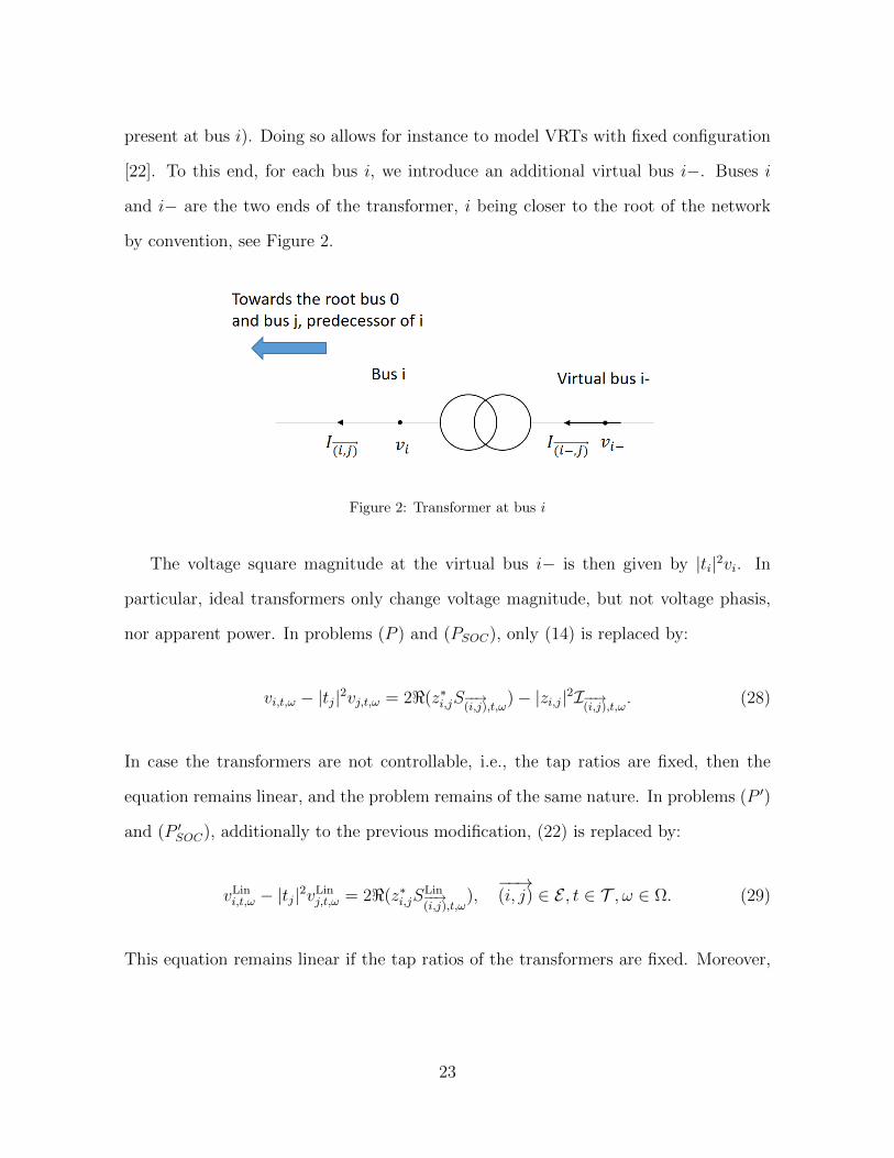
present at bus i). Doing so allows for instance to model VRTs with fixed configuration
[22]. To this end, for each bus i, we introduce an additional virtual bus i−. Buses i
and i− are the two ends of the transformer, i being closer to the root of the network
by convention, see Figure 2.
Figure 2: Transformer at bus i
The voltage square magnitude at the virtual bus i− is then given by |ti|2vi. In
particular, ideal transformers only change voltage magnitude, but not voltage phasis,
nor apparent power. In problems (P ) and (PSOC), only (14) is replaced by:
vi,t,ω − |tj|2vj,t,ω = 2<(z∗i,jS−−→(i,j),t,ω)− |zi,j|2I−−→(i,j),t,ω
. (28)
In case the transformers are not controllable, i.e., the tap ratios are fixed, then the
equation remains linear, and the problem remains of the same nature. In problems (P ′)
and (P ′SOC), additionally to the previous modification, (22) is replaced by:
vLini,t,ω − |tj|2vLin
j,t,ω = 2<(z∗i,jSLin−−→(i,j),t,ω
),−−→(i, j) ∈ E , t ∈ T , ω ∈ Ω. (29)
This equation remains linear if the tap ratios of the transformers are fixed. Moreover,
23

the last equation in (24) is replaced by:
vLini,t,ω − |tj|2vLin
j,t,ω = 2<(z∗i,jSLin−−→(i,j),t,ω
),−−→(i, j) ∈ E .
Propositions 1 and 2 remain valid in the setting of uncontrollable transformers, by small
adaptations of the proofs. Line 12 of Algorithm 1 is modified as:
v′i,t,ω ← |tj|2v′j,t,ω + 2<(z∗i,jS′−−→(i,j),t,ω
)− |zi,j|2I ′−−→(i,j),t,ω
.
Lemmas 1, 2, Corollary 1, Theorems 1, 2 and 3 remain valid in the case of uncontrollable
transformers.
5.2. Extension to controllable VRT
Considering tap ratios of transformers as decision variables introduce non-linearity
(and non-convexity) in Constraints (28) and (29). Extension of our results to this case
is an interesting perspective of our work left for future research. Let us provide some
intuition on a possible modeling procedure though, inspired by [22, 24]. If the tap ratios
take value in a continuous interval [tmini , tmaxi ] ⊂ (0,+∞), then (P ) (resp. (PSOC)) is
unchanged up to introduction to additional decision variables w−−→(i,j),t,ω
for all−−→(i, j) ∈ E ,
t ∈ T , ω ∈ Ω and Constraint (14) is replaced by:
vi,t,ω − wj,t,ω = 2<(z∗i,jS−−→(i,j),t,ω)− |zi,j|2I−−→(i,j),t,ω
,−−→(i, j) ∈ E , t ∈ T , ω ∈ Ω,
|tmini |2vi,t,ω ≤ wi,t,ω ≤ |tmaxi |2vi,t,ω, i ∈ B, t ∈ T , ω ∈ Ω.
24

For (P ′) and (P ′SOC), one needs other additional decision variables wLin−−→(i,j),t,ω
and Con-
straint (22) is replaced by:
vLini,t,ω − wLin
i,t,ω = 2<(z∗i,jSLin−−→(i,j),t,ω
),−−→(i, j) ∈ E , t ∈ T , ω ∈ Ω,
|tmini |2vLini,t,ω ≤ wLin
i,t,ω ≤ |tmaxi |2vLini,t,ω, i ∈ B, t ∈ T , ω ∈ Ω.
Extension of our results to this setting require an adaptation of step 12 of Algorithm 1
in order to give an explicit updating rule for w and v. In the case where the tap ratios
of transformers are decision variables with value in (finite) discrete sets, it is possible to
model (P ) and (P ′) as Mixed-Integer Non-Linear Programming problems and (PSOC)
and (P ′SOC) and Mixed-Integer Second Order Cone Programming problems, see [22, 24].
Our results can be applied in at the leaves of a branch-and-bound tree, when all tap
ratios of VRTs are fixed.
5.3. Other voltage regulation devices
Introducing capacitor banks in the model requires the modeling of nodal shunt
elements, which requires in turn a modification of the Branch Flow Model [8]. In
particular, (12) is replaced by:
S−−→(i,j),t,ω
=∑−−→(k,i)∈E
(S−−→(k,i),t,ω
− zk,iI−−→(k,i),t,ω) + yshi vi,t,ω + si,t,ω. (30)
Similarly, (20) is replaced by:
SLin−−→(i,j),t,ω
=∑−−→(k,i)∈E
SLin−−→(k,i),t,ω
+ yshi vLini,t,ω + si,t,ω. (31)
Due to the additional dependency of S and SLin on v and vLin respectively, it remains
unclear whether the key Lemmas 1 and 2 remain valid, even under some sign conditions
25

on the real and imaginary part of their associated admittance. This is due to the fact
that the proofs of these lemmas relied on the tree structure of the network and on (12)
and (20) being independent from v, which allowed to directly prove comparison relation
for apparent power. Therefore, whether our results are valid or not with capacitor banks
remains an open question. On the other hand, SVCs and STATCOMs can inject or
absorb reactive power at the buses of the network and our model already allows this
possibility. Such devices can thus be incorporated in the model while preserving our
results.
5.4. Extension to unbalanced multi-phase networks
In the multi-phase setting, the natural convex relaxation of the problem becomes a
SDP relaxation [22, 24, 25] and the non-convex equality constraints (15) are replaced
by rank-one constraints for 6 x 6 matrices for three-phase networks. Thus, we do not
expect our fixed point procedure (consisting in repeating an adaptation of Algorithm
1 until convergence) to yield solutions satisfying such rank conditions. Or at least, we
do not expect to be able to prove it easily. This is left for further research.
6. Case studies and numerical illustration
This numerical study is implemented using Matlab R2018b combined with YALMIP
R20200116, interfaced with conic solver Gurobi 9.0.0 with an Intel-Core i7 PC at 2.1
GHz with 16 Go memory.
6.1. Network topology
We consider a distribution network on the Southern California Edison system with
56 buses [13]. A visualization of the network before relabeling the buses is given in
Figure 3.
26
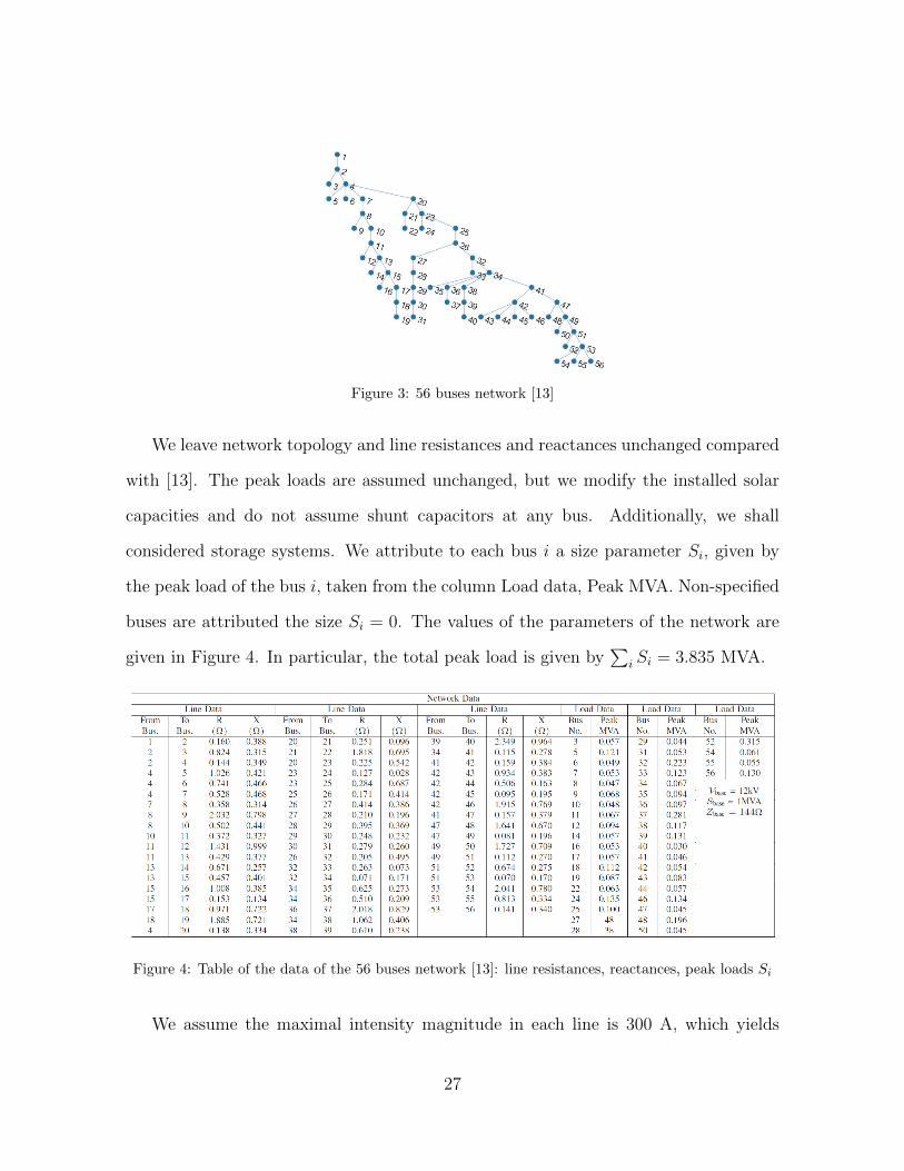
Figure 3: 56 buses network [13]
We leave network topology and line resistances and reactances unchanged compared
with [13]. The peak loads are assumed unchanged, but we modify the installed solar
capacities and do not assume shunt capacitors at any bus. Additionally, we shall
considered storage systems. We attribute to each bus i a size parameter Si, given by
the peak load of the bus i, taken from the column Load data, Peak MVA. Non-specified
buses are attributed the size Si = 0. The values of the parameters of the network are
given in Figure 4. In particular, the total peak load is given by∑
i Si = 3.835 MVA.
Figure 4: Table of the data of the 56 buses network [13]: line resistances, reactances, peak loads Si
We assume the maximal intensity magnitude in each line is 300 A, which yields
27

the bound I−−→(i,j)
= 90000 A2. We accept 5% deviations of voltage magnitude from
the reference value, i.e., v−−→(i,j)
= (0.95)2 p.u. and v−−→(i,j)
= (1.05)2 p.u. We assume also
S−−→(i,j)
= 5 MVA.
6.2. Discussion about other electronics devices
More generally, incorporating devices which only modify the bounds on power injec-
tions at buses except the reference (like storage systems, flexible consumption, energy
conversion systems...) do not make Theorem 1 invalid. Besides, a priori conditions
guaranteeing a vanishing relaxation gap (see Theorem 3) should be verified with the
updated bounds on power injections. For devices which directly impact voltage or
intensity magnitude or link them with power injections like shunt capacitors (see the
model of [13]) or transformers, one should extend the analysis developed above to check
if similar results may hold under further assumptions.
6.3. Exogenous residual demand
We consider an exogenous demand profile at node i and for time t given by the
difference between a deterministic consumption profile and a solar power production
profile
sdi,t,ω = sconsi,t − psol
i,t,ω.
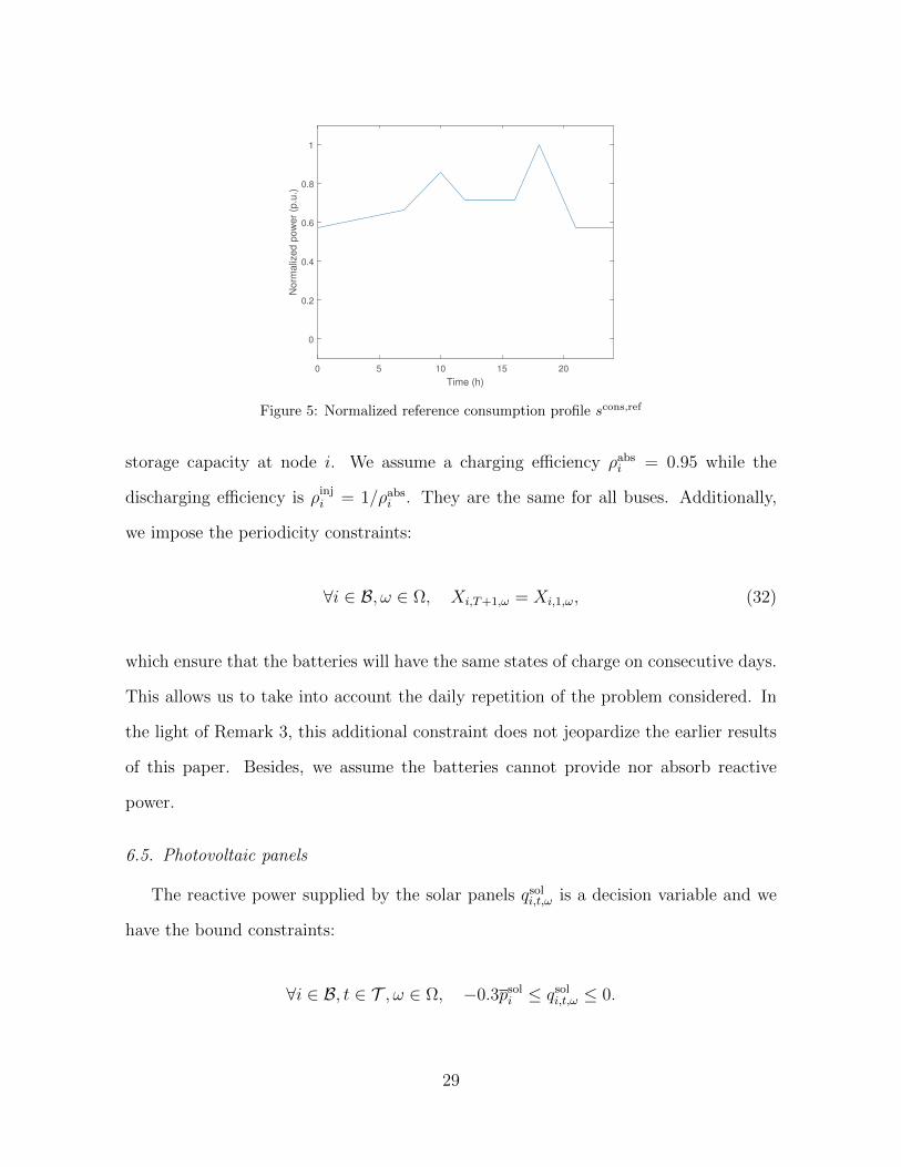
The consumption profiles are given by sconsi,t = scons,ref
t1+i0.2√1+(0.2)2
Si, i.e., the consumption
at each node i is proportional to a reference deterministic evolution scons,ref (independent
from i) represented in Figure 5 and the size parameter Si.
6.4. Batteries
We assume pinji (resp. pabs
i ) represents the power supplied (absorbed) by the battery
at bus i, at time step t ∈ T , for scenario ω ∈ Ω. We assume each battery can be
charged/discharged in τ =2 hours, i.e., pinji = pabs
i = Xi
τwhere X i denotes the installed
28
0 5 10 15 20
Time (h)
0
0.2
0.4
0.6
0.8
1
No
rma
lize
d p
ow
er
(p.u
.)
Figure 5: Normalized reference consumption profile scons,ref
storage capacity at node i. We assume a charging efficiency ρabsi = 0.95 while the
discharging efficiency is ρinji = 1/ρabs
i . They are the same for all buses. Additionally,
we impose the periodicity constraints:
∀i ∈ B, ω ∈ Ω, Xi,T+1,ω = Xi,1,ω, (32)
which ensure that the batteries will have the same states of charge on consecutive days.
This allows us to take into account the daily repetition of the problem considered. In
the light of Remark 3, this additional constraint does not jeopardize the earlier results
of this paper. Besides, we assume the batteries cannot provide nor absorb reactive
power.
6.5. Photovoltaic panels
The reactive power supplied by the solar panels qsoli,t,ω is a decision variable and we
have the bound constraints:
∀i ∈ B, t ∈ T , ω ∈ Ω, −0.3psoli ≤ qsol
i,t,ω ≤ 0.
29

6.6. First use case: diffuse energy storage systems and solar production
We assume the total installed capacity of batteries is Xtot
= 1 MWh. Each bus
i ∈ B is equipped with a battery with maximal energy capacity proportional to the
peak load Si of the bus X i = Si∑i∈B Si
Xtot
. The total installed solar capacity is denoted
psol,tot and its value will be set to different levels later on. Each bus i is equipped
with photovoltaic panels with maximal capacity proportional to the size Si of the bus,
i.e., psoli = Si∑
i∈B Sipsol,tot. Let us show that for psol,tot inferior to some threshold value,
(24)-(25) hold. To this end, we consider the upper bound si = Si∑i∈B Si
(psol,tot + X
tot
τ
)−
0.55 1+i0.2√1+(0.2)2
Si on the power injections at bus i, valid for any time and any scenario
tree, where we used the fact that 0.55 ≤ mint∈T scons,reft . Let us consider the linear
program (LP ):
maxpsol,tot,SLin,vLin
psol,tot
s.t. SLin−−→(i,j)
=∑−−→(k,i)∈E
SLin−−→(k,i)− 0.55
1 + i0.2√1 + (0.2)2
Si
+Si∑i∈B Si
(psol,tot +
Xtot
τ
),
−−→(i, j) ∈ E ,
vLin0 = 1,
vLini − vLin
j = 2<(z∗i,jSLin−−→(i,j)
),−−→(i, j) ∈ E .
vLini ≤ vi, i ∈ B,
<(z∗k,lSLin−−→(i,j)
) ≤ 0,−−→(i, j) ∈ E ,
−−→(k, l) ∈ Ei.
The projection of the feasibility set of this optimization problem along the first compo-
nent psol,tot is either empty, R if val(LP ) = +∞ or an interval of the form (−∞, val(LP )].
By solving it numerically, we find val(LP ) = 1.7023, which shows that for psol,tot ≤
30
1.7023 MW, (24)-(25) are satisfied and therefore, by Theorem 3, (P ) has no relaxation
gap, provided that the assumptions of Theorem 1 hold. This shows that the absence of a
relaxation gap can be proved under more realistic assumptions than over-generation [7]
or load over-satisfaction [8], and in a general multi-stage stochastic setting, unlike [11]
which considers a deterministic model. In particular, this condition does not depend
on the time grid (τt)t or on the scenario tree.
6.7. Second use case: concentrated energy storage systems and solar production
In this second example, we assume that there is no battery and that only buses 7
and 20 are equipped with PV panels. The installed capacities are respectively denoted
by psol7 and psol
20 . We consider the upper bound si = psoli − 0.55 1+i0.2√
1+(0.2)2Si on the power
injections at bus i, valid for any time and any scenario tree, where we used the fact
that 0.55 ≤ mint∈T scons,reft . We want to maximize the installed solar capacity at both
buses while guaranteeing an a priori vanishing relaxation gap by enforcing (24)-(25) to
hold. This yields the linear program (LP ′):
maxpsol7 ,psol20 ,S
Lin,vLinpsol
7 + psol20 ,
s.t. SLin−−→(i,j)
=∑−−→(k,i)∈E
SLin−−→(k,i)
+ psoli − 0.55
1 + i0.2√1 + (0.2)2
Si,−−→(i, j) ∈ E ,
vLin0 = 1,
vLini − vLin
j = 2<(z∗i,jSLin−−→(i,j)
),−−→(i, j) ∈ E .
vLini ≤ vi, i ∈ B,
<(z∗k,lSLin−−→(i,j)
) ≤ 0,−−→(i, j) ∈ E ,
−−→(k, l) ∈ Ei,
psol7 ≥ 0,
psol20 ≥ 0.
31
Then the maximal installed solar capacity is given by psol,tot = psol7 + psol
20 = 2.0851 MW
with psol7 = 0.4399 MW and psol
20 = 1.6452 MW. Therefore, for any values of psol7 ≤ 0.4399
MW and psol20 ≤ 1.6452 MW, (24)-(25) hold and therefore, by Theorem 3, (P ) has no
relaxation gap, provided that the assumptions of Theorem 1 hold. This is true for any
choice of time grid and scenario tree, provided scons,reft ≥ 0.55 for any t ∈ T .
6.8. Numerical study of the upper bound on the relaxation gap
From now on, we numerically investigate the upper bound on the relaxation gap
derived in Theorem 2 on the first use case with diffuse energy storage systems and
solar production, see 6.6. We consider higher levels of installed solar capacity so that
assumptions of Theorem 3 do not hold anymore. We need to specify an optimization
window and a scenario tree.
6.8.1. Time grid considered
We consider an optimization window of 31 hours, divided into T + 1 = 9 sub-
intervals. Each time step t corresponds to a time interval in the model [τt, τt+1]. The
correspondence between t and τt is given in Table 2. One could consider instead a
finer time grid, with step lengths of 15 minutes or 1 hour, which is most common in
practice. However, as discussed below, the number of scenarios is generally exponential
in the number of “branching points” of the scenario tree, hence, to avoid a blow up
of the size of the optimization problem, one needs to use scenario trees branching at
time steps from a coarser time grid. However, this coarse grid need not be uniformly
distributed. Here, since the scenario tree provides a quantization of the randomness
of solar production, we use 2-hours steps from 10 am to 6 pm, 3-hours steps from 7
to 10 am and from 9 pm to midnight the next day, and a single step of 7 hours for
all the night from midnight to 7 am. We also emphasize that our theoretical results
regarding the relaxation gap do not depend directly on the choice of time discretization
32
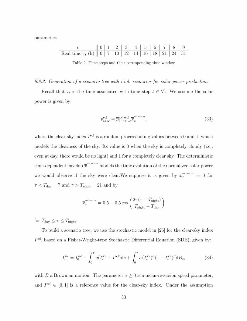
parameters.
t 0 1 2 3 4 5 6 7 8 9Real time τt (h) 0 7 10 12 14 16 18 21 24 31
Table 2: Time steps and their corresponding time window
6.8.2. Generation of a scenario tree with i.i.d. scenarios for solar power production
Recall that τt is the time associated with time step t ∈ T . We assume the solar
power is given by:
psoli,t,ω = psol
i Isolτt,ωx
sol,norm
τt , (33)
where the clear-sky index Isol is a random process taking values between 0 and 1, which
models the clearness of the sky. Its value is 0 when the sky is completely cloudy (i.e.,
even at day, there would be no light) and 1 for a completely clear sky. The deterministic
time-dependent envelop xsol,norm
models the time evolution of the normalized solar power
we would observe if the sky were clear.We suppose it is given by xsol,norm
τ = 0 for
τ < Tday = 7 and τ > Tnight = 21 and by
xsol,norm
τ = 0.5− 0.5 cos
(2π(τ − Tnight)
Tnight − Tday
)
for Tday ≤ τ ≤ Tnight.
To build a scenario tree, we use the stochastic model in [26] for the clear-sky index
Isol, based on a Fisher-Wright-type Stochastic Differential Equation (SDE), given by:
Isolτ = Isol
0 −∫ τ
0
a(Isols − Iref)ds+
∫ τ
0
σ(Isols )α(1− Isol
s )βdBs, (34)
with B a Brownian motion. The parameter a ≥ 0 is a mean-reversion speed parameter,
and Iref ∈ [0, 1] is a reference value for the clear-sky index. Under the assumption
33
a ≥ 0, α, β ≥ 0.5, this SDE has a unique strong solution with values in [0, 1] almost
surely, see [26].
The branching structure of the scenario tree is characterized by pre-specified vector
(Ct)t∈T where Ct corresponds to the number of children nodes of a node at stage t. In
particular, the total number of scenarios is given by N =∏T
t=1 Ct. Given a structure of
a scenario tree, we use the quantile-based Algorithm 2 with parameters given in Table
3 to instantiate the values of solar irradiance at the nodes of the scenario tree. Each
scenario is assigned probability 1/N , which is consistent with the fact that we consider
evenly spaced quantiles for the values of successors of each node.
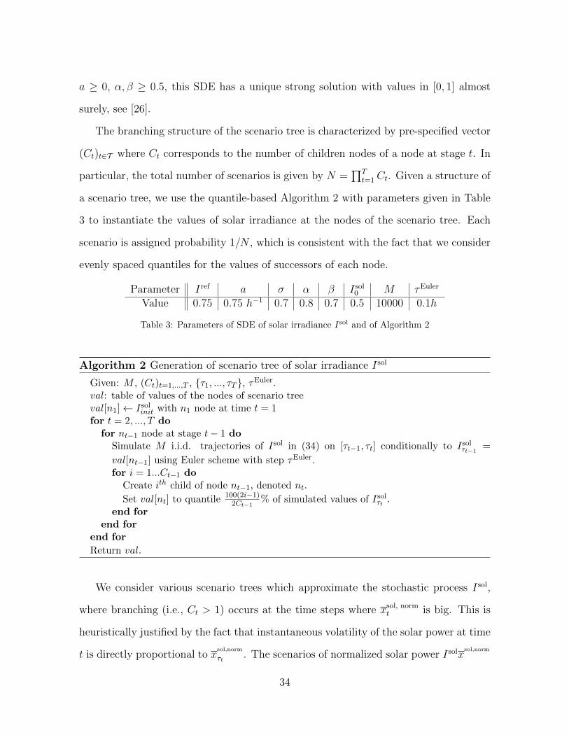
Parameter Iref a σ α β Isol0 M τEuler
Value 0.75 0.75 h−1 0.7 0.8 0.7 0.5 10000 0.1h
Table 3: Parameters of SDE of solar irradiance Isol and of Algorithm 2
Algorithm 2 Generation of scenario tree of solar irradiance Isol
Given: M , (Ct)t=1,...,T , τ1, ..., τT , τEuler.val: table of values of the nodes of scenario treeval[n1]← Isol
init with n1 node at time t = 1for t = 2, ..., T do
for nt−1 node at stage t− 1 doSimulate M i.i.d. trajectories of Isol in (34) on [τt−1, τt] conditionally to Isol
τt−1=
val[nt−1] using Euler scheme with step τEuler.for i = 1...Ct−1 do
Create ith child of node nt−1, denoted nt.
Set val[nt] to quantile 100(2i−1)2Ct−1
% of simulated values of Isolτt .
end forend for
end for
Return val.
We consider various scenario trees which approximate the stochastic process Isol,
where branching (i.e., Ct > 1) occurs at the time steps where xsol, normt is big. This is
heuristically justified by the fact that instantaneous volatility of the solar power at time
t is directly proportional to xsol,norm
τt . The scenarios of normalized solar power Isolxsol,norm
34
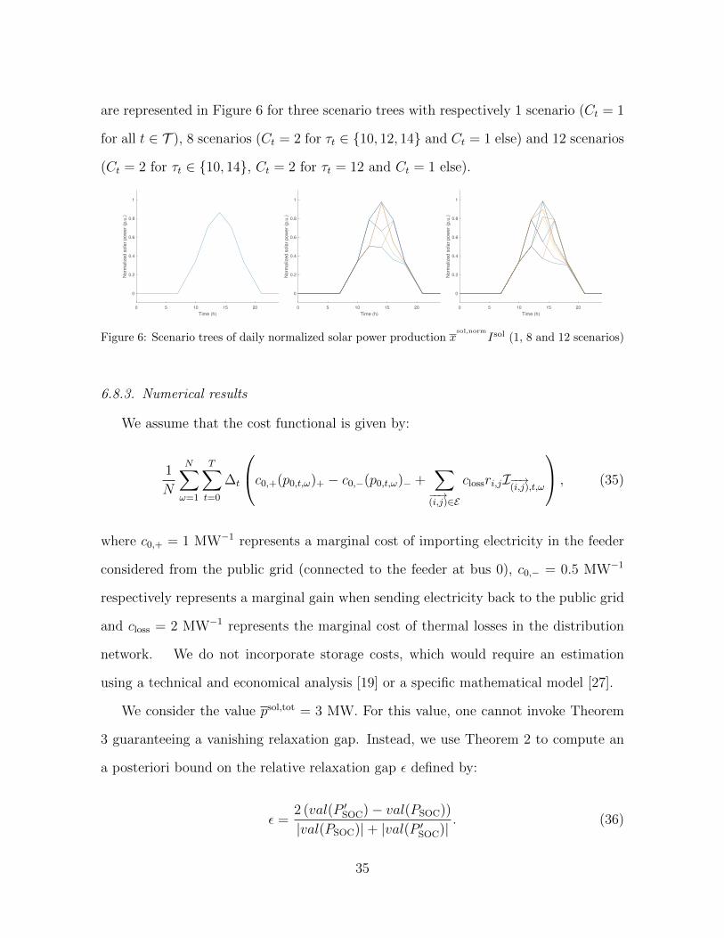
are represented in Figure 6 for three scenario trees with respectively 1 scenario (Ct = 1
for all t ∈ T ), 8 scenarios (Ct = 2 for τt ∈ 10, 12, 14 and Ct = 1 else) and 12 scenarios
(Ct = 2 for τt ∈ 10, 14, Ct = 2 for τt = 12 and Ct = 1 else).
0 5 10 15 20
Time (h)
0
0.2
0.4
0.6
0.8
1
Norm
aliz
ed s
ola
r pow
er
(p.u
.)
0 5 10 15 20
Time (h)
0
0.2
0.4
0.6
0.8
1
Norm
aliz
ed s
ola
r pow
er
(p.u
.)
0 5 10 15 20
Time (h)
0
0.2
0.4
0.6
0.8
1
Norm
aliz
ed s
ola
r pow
er
(p.u
.)
Figure 6: Scenario trees of daily normalized solar power production xsol,norm
Isol (1, 8 and 12 scenarios)
6.8.3. Numerical results
We assume that the cost functional is given by:
1
N
N∑ω=1
T∑t=0
∆t
c0,+(p0,t,ω)+ − c0,−(p0,t,ω)− +∑−−→(i,j)∈E
clossri,jI−−→(i,j),t,ω
, (35)
where c0,+ = 1 MW−1 represents a marginal cost of importing electricity in the feeder
considered from the public grid (connected to the feeder at bus 0), c0,− = 0.5 MW−1
respectively represents a marginal gain when sending electricity back to the public grid
and closs = 2 MW−1 represents the marginal cost of thermal losses in the distribution
network. We do not incorporate storage costs, which would require an estimation
using a technical and economical analysis [19] or a specific mathematical model [27].
We consider the value psol,tot = 3 MW. For this value, one cannot invoke Theorem
3 guaranteeing a vanishing relaxation gap. Instead, we use Theorem 2 to compute an
a posteriori bound on the relative relaxation gap ε defined by:
ε =2 (val(P ′SOC)− val(PSOC))
|val(PSOC)|+ |val(P ′SOC)|. (36)
35
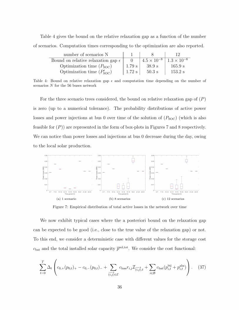
Table 4 gives the bound on the relative relaxation gap as a function of the number
of scenarios. Computation times corresponding to the optimization are also reported.
number of scenarios N 1 8 12Bound on relative relaxation gap ε 0 4.5× 10⁻⁸ 1.3× 10⁻⁶
Optimization time (PSOC) 1.79 s 38.9 s 165.9 sOptimization time (P ′SOC) 1.72 s 50.3 s 153.2 s
Table 4: Bound on relative relaxation gap ε and computation time depending on the number ofscenarios N for the 56 buses network
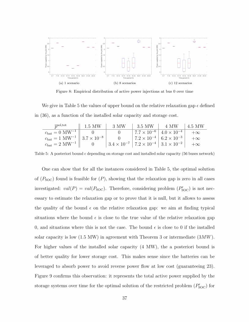
For the three scenario trees considered, the bound on relative relaxation gap of (P )
is zero (up to a numerical tolerance). The probability distributions of active power
losses and power injections at bus 0 over time of the solution of (PSOC) (which is also
feasible for (P )) are represented in the form of box-plots in Figures 7 and 8 respectively.
We can notice than power losses and injections at bus 0 decrease during the day, owing
to the local solar production.
0-7 7-10 10-12 12-14 14-16 16-18 18-21 21-24 24-31
Time period (h)
0
0.01
0.02
0.03
0.04
0.05
0.06
Po
we
r lo
sse
s (
MW
)
(a) 1 scenario
0-7 7-10 10-12 12-14 14-16 16-18 18-21 21-24 24-31
Time period (h)
0
0.01
0.02
0.03
0.04
0.05
0.06
Po
we
r lo
sse
s (
MW
)
(b) 8 scenarios
0-7 7-10 10-12 12-14 14-16 16-18 18-21 21-24 24-31
Time period (h)
0
0.01
0.02
0.03
0.04
0.05
0.06
Po
we
r lo
sse
s (
MW
)
(c) 12 scenarios
Figure 7: Empirical distribution of total active losses in the network over time
We now exhibit typical cases where the a posteriori bound on the relaxation gap
can be expected to be good (i.e., close to the true value of the relaxation gap) or not.
To this end, we consider a deterministic case with different values for the storage cost
cbat and the total installed solar capacity psol,tot. We consider the cost functional:
T∑t=0
∆t
c0,+(p0,t)+ − c0,−(p0,t)− +∑−−→(i,j)∈E
clossri,jI−−→(i,j),t+∑i∈B
cbat(pinji,t + pabs
i,t )
. (37)
36
0-7 7-10 10-12 12-14 14-16 16-18 18-21 21-24 24-31
Time period (h)
0
0.5
1
1.5
2
2.5
3
Po
we
r su
pp
lied
by t
he
grid
(M
W)
(a) 1 scenario
0-7 7-10 10-12 12-14 14-16 16-18 18-21 21-24 24-31
Time period (h)
0
0.5
1
1.5
2
2.5
3
Po
we
r su
pp
lied
by t
he
grid
(M
W)
(b) 8 scenarios
0-7 7-10 10-12 12-14 14-16 16-18 18-21 21-24 24-31
Time period (h)
0
0.5
1
1.5
2
2.5
3
Po
we
r su
pp
lied
by t
he
grid
(M
W)
(c) 12 scenarios
Figure 8: Empirical distribution of active power injections at bus 0 over time
We give in Table 5 the values of upper bound on the relative relaxation gap ε defined
in (36), as a function of the installed solar capacity and storage cost.
psol,tot 1.5 MW 3 MW 3.5 MW 4 MW 4.5 MWcbat = 0 MW−1 0 0 7.7× 10⁻⁶ 4.0× 10⁻⁴ +∞cbat = 1 MW−1 3.7× 10⁻⁸ 0 7.2× 10⁻⁴ 6.2× 10⁻³ +∞cbat = 2 MW−1 0 3.4× 10⁻⁷ 7.2× 10⁻⁴ 3.1× 10⁻² +∞
Table 5: A posteriori bound ε depending on storage cost and installed solar capacity (56 buses network)
One can show that for all the instances considered in Table 5, the optimal solution
of (PSOC) found is feasible for (P ), showing that the relaxation gap is zero in all cases
investigated: val(P ) = val(PSOC). Therefore, considering problem (P ′SOC) is not nec-
essary to estimate the relaxation gap or to prove that it is null, but it allows to assess
the quality of the bound ε on the relative relaxation gap: we aim at finding typical
situations where the bound ε is close to the true value of the relative relaxation gap
0, and situations where this is not the case. The bound ε is close to 0 if the installed
solar capacity is low (1.5 MW) in agreement with Theorem 3 or intermediate (3MW ).
For higher values of the installed solar capacity (4 MW), the a posteriori bound is
of better quality for lower storage cost. This makes sense since the batteries can be
leveraged to absorb power to avoid reverse power flow at low cost (guaranteeing 23).
Figure 9 confirms this observation: it represents the total active power supplied by the
storage systems over time for the optimal solution of the restricted problem (P ′SOC) for
37
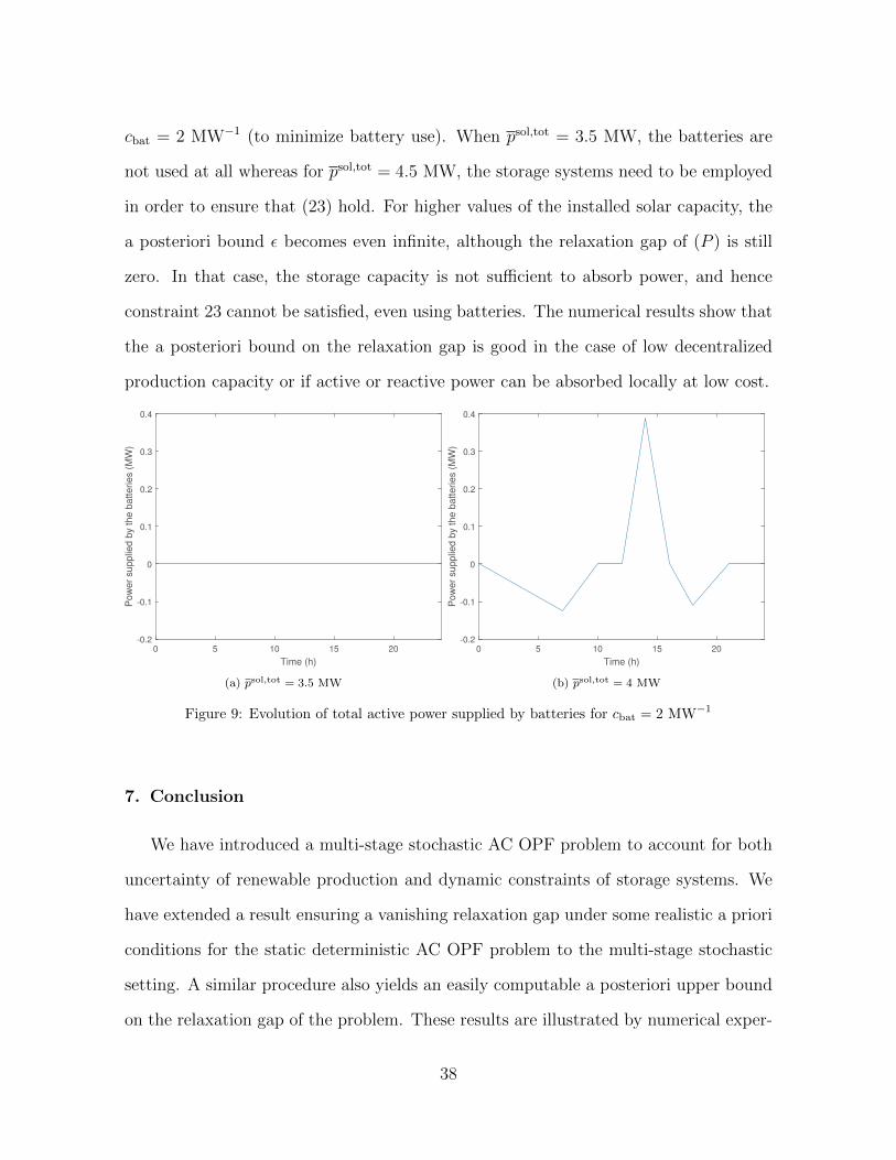
cbat = 2 MW−1 (to minimize battery use). When psol,tot = 3.5 MW, the batteries are
not used at all whereas for psol,tot = 4.5 MW, the storage systems need to be employed
in order to ensure that (23) hold. For higher values of the installed solar capacity, the
a posteriori bound ε becomes even infinite, although the relaxation gap of (P ) is still
zero. In that case, the storage capacity is not sufficient to absorb power, and hence
constraint 23 cannot be satisfied, even using batteries. The numerical results show that
the a posteriori bound on the relaxation gap is good in the case of low decentralized
production capacity or if active or reactive power can be absorbed locally at low cost.
0 5 10 15 20
Time (h)
-0.2
-0.1
0
0.1
0.2
0.3
0.4
Pow
er
supplie
d b
y the b
atteries (
MW
)
(a) psol,tot = 3.5 MW
0 5 10 15 20
Time (h)
-0.2
-0.1
0
0.1
0.2
0.3
0.4
Pow
er
supplie
d b
y the b
atteries (
MW
)
(b) psol,tot = 4 MW
Figure 9: Evolution of total active power supplied by batteries for cbat = 2 MW−1
7. Conclusion
We have introduced a multi-stage stochastic AC OPF problem to account for both
uncertainty of renewable production and dynamic constraints of storage systems. We
have extended a result ensuring a vanishing relaxation gap under some realistic a priori
conditions for the static deterministic AC OPF problem to the multi-stage stochastic
setting. A similar procedure also yields an easily computable a posteriori upper bound
on the relaxation gap of the problem. These results are illustrated by numerical exper-
38
iments on a realistic distribution network with local generation and storage systems.
Possible extensions of this work would be to consider three-phase unbalanced networks,
controllable VRT and capacitor banks.
Acknowledgments
This work has benefited from several supports: Siebel Energy Institute (Calls for
Proposals #2, 2016), ANR project CAESARS (ANR-15-CE05-0024), Association Na-
tionale de la Recherche Technique (ANRT), Electricite De France (EDF), Finance for
Energy Market (FiME) Lab (Institut Europlace de Finance). The authors would like
to thank Riadh Zorgati, Mathieu Caujolle and Bhargav Swaminathan for fruitful dis-
cussion. They also thank the reviewers for their detailed comments.
References
[1] S. Low, Convex Relaxation of Optimal Power Flow - part 1: Formulations and
equivalence, IEEE Transactions on Control of Network Systems 1 (1) (2014) 15–
27. doi:10.1109/TCNS.2014.2309732.
[2] T. Ding, R. Lu, Y. Yang, F. Blaabjerg, A condition of equivalence between Bus In-
jection and Branch Flow Models in radial networks, IEEE Transactions on Circuits
and Systems II: Express Briefs 67 (3) (2020) 536–540.
[3] D. Bienstock, A. Verma, Strong NP-hardness of AC power flows feasibility, Oper-
ations Research Letters 47 (6) (2019) 494–501.
[4] J. Lavaei, S. H. Low, Zero duality gap in Optimal Power Flow problem, IEEE
Transactions on Power Systems 27 (1) (2011) 92–107.
[5] D. K. Molzahn, I. A. Hiskens, et al., A survey of relaxations and approximations
of the power flow equations, Now Publishers, 2019.
39
[6] F. Zohrizadeh, C. Josz, M. Jin, R. Madani, J. Lavaei, S. Sojoudi, A survey on
conic relaxations of Optimal Power Flow problem, European journal of operational
research 287 (2020) 391–409.
[7] S. Sojoudi, J. Lavaei, Physics of power networks makes hard optimization problems
easy to solve, in: 2012 IEEE Power and Energy Society General Meeting, IEEE,
2012, pp. 1–8. doi:10.1109/PESGM.2012.6345272.
[8] M. Farivar, S. H. Low, Branch flow model: Relaxations and convexification—part
i, IEEE Transactions on Power Systems 28 (3) (2013) 2554–2564.
[9] L. Gan, N. Li, U. Topcu, S. Low, On the exactness of convex relaxation for Optimal
Power Flow in tree networks, in: 2012 IEEE 51st IEEE Conference on Decision
and Control (CDC), IEEE, 2012, pp. 465–471.
[10] L. Gan, N. Li, U. Topcu, S. H. Low, Exact convex relaxation of Optimal Power
Flow in radial networks, IEEE Transactions on Automatic Control 60 (1) (2014)
72–87.
[11] S. Huang, Q. Wu, J. Wang, H. Zhao, A sufficient condition on convex relaxation
of AC Optimal Power Flow in distribution networks, IEEE Transactions on Power
Systems 32 (2) (2016) 1359–1368.
[12] G. C. Pflug, A. Pichler, Multistage stochastic optimization, Springer, 2014.
[13] M. Farivar, R. Neal, C. Clarke, S. Low, Optimal inverter var control in distribution
systems with high pv penetration, in: 2012 IEEE Power and Energy Society general
meeting, IEEE, 2012, pp. 1–7.
[14] E. Grover-Silva, R. Girard, G. Kariniotakis, Optimal sizing and placement of dis-
40
tribution grid connected battery systems through an SOCP Optimal Power Flow
algorithm, Applied Energy 219 (2018) 385–393.
[15] L. Roald, G. Andersson, Chance-constrained AC Optimal Power Flow: Reformula-
tions and efficient algorithms, IEEE Transactions on Power Systems 33 (3) (2017)
2906–2918.
[16] M. Vrakopoulou, M. Katsampani, K. Margellos, J. Lygeros, G. Andersson, Prob-
abilistic security-constrained AC Optimal Power Flow, in: 2013 IEEE Grenoble
Conference, IEEE, 2013, pp. 1–6.
[17] A. Venzke, L. Halilbasic, U. Markovic, G. Hug, S. Chatzivasileiadis, Convex re-
laxations of chance constrained AC Optimal Power Flow, IEEE Transactions on
Power Systems 33 (3) (2017) 2829–2841.
[18] L. Halilbasic, P. Pinson, S. Chatzivasileiadis, Convex relaxations and approxi-
mations of chance-constrained AC-OPF problems, IEEE Transactions on Power
Systems 34 (2) (2018) 1459–1470.
[19] B. P. Swaminathan, Operational planning of active distribution networks-convex
relaxation under uncertainty, Ph.D. thesis, Universite Grenoble Alpes (2017).
[20] R. A. Jabr, S. Karaki, J. A. Korbane, Robust multi-period OPF with storage and
renewables, IEEE Transactions on Power Systems 30 (5) (2014) 2790–2799.
[21] G. Sun, Y. Li, S. Chen, Z. Wei, S. Chen, H. Zang, Dynamic stochastic Optimal
Power Flow of wind power and the electric vehicle integrated power system con-
sidering temporal-spatial characteristics, Journal of Renewable and Sustainable
Energy 8 (5) (2016) 053309.
41
[22] Y. Liu, J. Li, L. Wu, T. Ortmeyer, Chordal relaxation based ACOPF for unbal-
anced distribution systems with ders and voltage regulation devices, IEEE Trans-
actions on Power Systems 33 (1) (2017) 970–984.
[23] M. Baran, F. F. Wu, Optimal sizing of capacitors placed on a radial distribution
system, IEEE Transactions on Power Delivery 4 (1) (1989) 735–743.
[24] Y. Liu, J. Li, L. Wu, Coordinated optimal network reconfiguration and voltage
regulator/der control for unbalanced distribution systems, IEEE Transactions on
Smart Grid 10 (3) (2018) 2912–2922.
[25] L. Gan, S. H. Low, Convex relaxations and linear approximation for Optimal
Power Flow in multiphase radial networks, in: 2014 Power Systems Computation
Conference, IEEE, 2014, pp. 1–9.
[26] J. Badosa, E. Gobet, M. Grangereau, D. Kim, Day-ahead probabilistic forecast
of solar irradiance: a Stochastic Differential Equation approach, in: P. Drobin-
ski, M. Mougeot, D. Picard, R. Plougonven, P. Tankov (Eds.), Renewable Energy:
Forecasting and Risk Management, Springer Proceedings in Mathematics & Statis-
tics, 2018, Ch. 4, pp. 73–93.
[27] P. Carpentier, J.-P. Chancelier, M. De Lara, T. Rigaut, Algorithms for two-time
scales stochastic optimization with applications to long term management of energy
storage, eprint hal-02013969 (2019).
42