Multi-variate Visualization of 3D Turbulent Flow Data

Sheng-Wen Wanga, Victoria Interrantea, Ellen Longmireb

aUniversity of Minnesota, 4-192 EE/CS Building, 200 Union St. SE, Minneapolis, MN bUniversity of Minnesota, 107 Akerman Hall, 110 Union St. SE, Minneapolis, MN

ABSTRACT

Turbulent flows play a critical role in many fields, yet our understanding of the fundamental physics of turbulence remains in its infancy. One of the long term goals in turbulence research is to develop an improved understanding of the dynamic evolution, interaction and organization of vortices in three-dimensional turbulent flow. However this task is complicated by the lack of a clear, mathematically precise definition of what a vortex is. We believe that the design of effective methods for vortex identification and segmentation in complicated turbulent flows can be facilitated by the clear, detailed visual presentation of the multiple scalar and vector quantities potentially relevant to the feature identification process. In this paper, we present several different methods aimed at facilitating the integrated understanding of a variety of local measures extracted from 3D multivariate flow data, including quantities, directions, and orientation. A key focus of our work is on the development of methods for illustrating the local relationships between scalar and vector values important to the vortex identification process such as vorticity, swirl, and velocity, along with their direction and magnitude. Our methods include the use of arrows and glyphs or 3D texture along with different color coding strategies. We demonstrate our methods on a range of data including 3D turbulent boundary flow data and time varying ring data. The variety of multi-variate visualization methods that we have developed has succeeded in supporting fluids researchers in their efforts to gain deeper insights into their data.

Keywords: Flow visualization, turbulent flow, vorticity, swirl

1. INTRODUCTION Flow Visualization has been an active research topic for several decades. The research in this field focuses on how to best represent turbulent flows to help researchers understand the mechanisms of fluid dynamics, as much is still unknown about the processes of vortex generation and interaction. In fluids research, the development of methods to robustly identify individual vortices in turbulent flow is an ongoing challenge. Attempts to identify and analyze individual eddy structures in turbulent flow are complicated by the difficulty of formulating a mathematically robust definition of what a vortex is. As a result, most current analysis efforts are forced to rely on statistical properties of the flow as a whole rather than on information derived from tracking the behavior of individual eddies. In support of our ultimate goal of facilitating the development of improved methods for vortex identification and tracking, we have implemented a suite of methods that support the integrated visual analysis of multiple local physical properties derived from turbulent flows. Our aim is to create tools that fluids researchers and others can use to obtain greater insight into the characteristics of, and relationships between, various potential feature descriptors in the flow, such as vorticity magnitude and direction, and swirl strength, in order to better inform the development of robust methods for identifying, quantifying, and tracking individual eddy structures in complex turbulent flows.

Our methods begin with the application of region-of-interest masking to the 3D data, based on a scalar measure of swirl strength, in order to de-clutter the display and allow attention to be concentrated on the areas of the flow where the turbulent motion is strongest. Within these regions, we then enable the use of a combination of LIC 3, 4 glyphs and other primitives to simultaneously visualize multiple local scalar and vector-valued features of the flow such as: the direction, orientation, and magnitude of vorticity and velocity vectors, along with swirl strength, orientation and direction. We demonstrate the use of our system on two set of flow data: a complex, 3D turbulent boundary flow and a simpler vortex ring dataset and we also provide videos illustrating the effects of using different methods to represent time-varying aspects of the flow. The first dataset consists of a single time step from a large, high Reynolds number (934), 3D turbulent channel flow obtained by direct numerical simulation (DNS). This data was generated by del Alamo et al. 18.

The second dataset represents a very high Reynolds number (2500), experimentally captured 3D time-varying flow with 70 time steps. It was provided by Daniel R. Troolin and Ellen K. Longmire 22, and it features vortex rings generated by driving pistons within cylinders.

2. RELATED WORK Flow visualization is one of the oldest and most-studied topics in the field of data visualization, and many techniques have been proposed for visualizing multiple variables in flow data. A popular categorization of these techniques, given by Laramee et al. 5, is: a) Direct flow visualization; b) Dense, texture-based flow visualization; c) Geometric flow visualization; and d) Feature-based flow visualization. Briefly, these approaches can be summarized as follows:

Direct flow visualization is a highly efficient and intuitive technique in which a simple arrow, or continuous color coding, is applied directly at each of the locations at which the data has been sampled, providing an overall picture of the flow dataset.

Texture-based flow visualization methods create a dense representation of a flow field by using high density texture patterns to depict information in the flows. The characteristics of the texture patterns can be varied to convey multivariate information.

Geometric flow visualization methods involve the use of geometric objects, such as streamlets, streamlines and isosurfaces, to represent basic quantities in the flow data. Some glyph-based methods can fall into this category.

Feature-based flow visualization relies on the use of complex, higher level features, such as critical points, separation surfaces, etc., to sparsely represent only the most important information about a flow. Feature-based methods can be used in conjunction with the other methods listed above to achieve a more dense representation within which important information is highlighted.

All of these approaches can be effective in representing either 2D or 3D flow data, although three-dimensional flows present some particular challenges to visualization because of the large amount of information they contain in a relatively compact space. Post et al. 10 discuss various feature extraction techniques for steady flows and present schemes for feature tracking and event detection in unsteady flows. Park et al. 11, among others, demonstrate how to visualize 3D flows based on geometric objects, including streamlines and pathlines. Because 3D flow data are so dense, methods for selectively emphasizing the most important parts of the flow, making them easy to see and understand, are particularly important. Park et al. discuss ways to overcome a variety of 3D visualization issues, such as occlusion, illumination, depth perception, etc., which usually exist with elongated geometric objects. Recent work by O. Mallo et al. 19 uses programmable graphics processing units to shade line bundles, significantly enhancing the perception of line direction in three-dimensional space in an efficient way. However, in the generation of streamlines, the initial seed points have to be carefully defined in order to effectively represent the essential flow features while avoiding excessive occlusion. Weiskopf et al. 12 propose a real-time technique for rendering 3D unsteady flow using 3D GPU-based texture advection. They also utilize numerous schemes for solving similar 3D visualization issues. However, the occlusion problems inherent in dense textures restricts the applicability of this method for certain applications. Laramee et al. 13 discuss ways to combine direct, geometric, and texture-based techniques to visualize the motion of 3D flows. Direct flow visualization is very simple to use, and generally intuitive, but it is not ideal for the visualization of an entire flow volume. Laramee et al. show that geometric and texture-based methods also generally have to be used carefully, to render the flows with maximal coverage only in the interesting regions. Early work by Loffelmann and Groller 23 demonstrates using threads of streamlets to visualizing a 3D flow field, which represents a trade-off between using a lower dimensional manifold for the display of structural information about the flow and geometric entities such as streamlines or stream surfaces for the direct representation of the flow data. Generally, a combination of different types of techniques provides a trade-off of their strengths and weaknesses and enables rendering a complex flow more effectively.

Recently, Jankun-Kelly et al. 21 developed an algorithm to identify individual vortices in complex vortex regions. Other research by Shafhitzel et al. 14 focuses on the visualization of particular features such as vortex structures in 3D flow fields. Their work uses isosurface techniques to extract structures of interest, which are then enhanced with other rendering methods, including a surface LIC method, color coding, and geometric flow visualization, to visualize vortices with their velocity field and other quantities. Urness et al. 15 propose color weaving and texture stitching methods to visualize multi-variate flow data. They combine different coloring and visual variation to convey multiple variables in

one image. However, the methods of Urness et al. are only applicable to 2D flow fields. Other efforts in the visualization of multi-variate scientific data, including scalars, vectors, and tensors, can be found in the review by Burger and Hauser16. Those authors conduct a systematic analysis of a number of different schemes in order to better understand how to most effectively apply them. It is often the case that particular methods are required for particular problems, so developing and selecting proper tools to effectively portray multi-variate information in complex 3D flows is still an important research topic.

3. IMPLEMENTATION There is keen need for visualizing interesting areas in a 3D turbulent flow and inspecting properties corresponding to multiple variables within those regions since the behaviors of these flow have not yet been well understood by scientists. In this section, we describe our efforts to help researchers to better understand the relationship between local measures of vorticity and other possible measures of swirling motion through the use of visualization methods involving 3D arrows, glyphs, geometric objects, and various color coding schemes. Our ultimate aim is to enable researchers to be able to use this information in developing more effective vortex identification algorithms.

3.1 LIC Glyph Method

!"#$%&'()*(+*'),%-%.,#/0.1

2"#3%)%-0,%#24#

5%6,7-%

8"#97:%-#90;:<')&

="#24#>?@

A"#B7,<')%#@-%0,'()

C"#?D%),'+E#?),%-%.,')&#

F-%0.

G"#F76'<'0-E#24#>?@

H"#@(<(-#@(D')&#+(-#

I%0,7-%.

CC"#$%)D%-')&

J"#B,K%-#24#

L'.70<#M-';','N%.

CO"#F)(,K%-#5';%#9,%:P%.

Q(

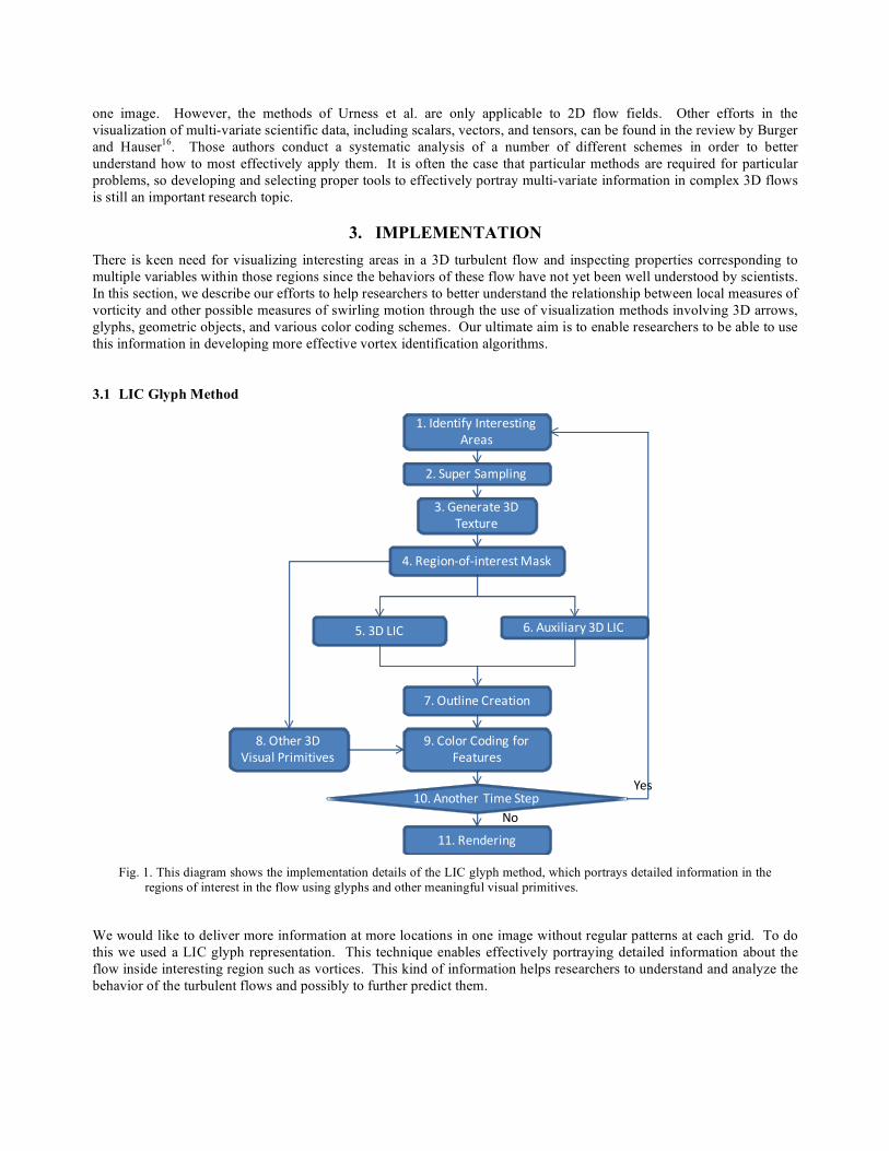
Fig. 1. This diagram shows the implementation details of the LIC glyph method, which portrays detailed information in the

regions of interest in the flow using glyphs and other meaningful visual primitives.

We would like to deliver more information at more locations in one image without regular patterns at each grid. To do this we used a LIC glyph representation. This technique enables effectively portraying detailed information about the flow inside interesting region such as vortices. This kind of information helps researchers to understand and analyze the behavior of the turbulent flows and possibly to further predict them.

The essential steps in our LIC glyph implementation are described in figure 4 and below.

1. Identifying Interesting Areas

We begin by identifying interesting regions in the flow, within which we wish to visualize detailed local scalar and vector information. These regions can be defined in a variety of ways. The simplest approach is to manually select a rectangular subset of grid cells that appears to contain potentially interesting flow features, based on a pre-visualization of a single scalar feature of the data such as swirl strength17, 1, 2. However, we have also implemented a method that automatically defines target regions for visualization around connected subsets of sample points where the swirl strength is above a specified threshold value. This design for automatically detecting and separating particular regions throughout the entire space assists researchers to identify the most important areas for investigation and also allows for further developing an automatic mechanism of this algorithm to define all of the interest targets.

2. Super Sampling

The next step is to super-sample the data within the target region, in order to provide sufficient resolution for the effective portrayal of local 3D scalar and vector data using glyphs. Both of the turbulent flow datasets we are working with are discrete, and in the turbulent channel flow dataset each of the thousands of critical regions in it may occupy only a few grid cells. In order to provide highly detailed information in these areas, a super sampling step is required to accommodate a reasonable number of high resolution glyphs distributed throughout each of the regions. However the level of super sampling has to be chosen carefully. A lower level of super sampling will provide higher efficiency performance, but the glyphs may not be capable of delivering finely enough detailed information. On the other hand, a higher level of super sampling enables conveying more information with more glyphs, but the computational efforts may be extremely large. Moreover, extremely high interpolation of the data may introduce unwanted side effects. Therefore, some tradeoff has to be made according to the computation speed, memory usage, and disk capacity.

3. Generate 3D Texture

In this step, we generate a 3D texture within the regions of interest, consisting of multiple spherically-shaped particles (Gaussian balls) seeded at randomly selected locations but maintaining a minimum separation, approximating a Poisson distribution. The purpose of this distributed particle placement is to prevent artifacts caused by particle conglomeration while providing an equal opportunity for every location to be occupied by a particle. Keeping the seed points apart by a certain distance is required to avoid the chance of overlapping particles. This has to be done carefully to maintain the particles still dense enough in the space.

4. Region-of-Interest Mask

We typically apply a region-of-interest mask to the input texture before conducting the LIC in order to reduce the number of particles and to preferentially emphasize the display of information in the areas of particularly strongly swirling flow. This step placed ahead of the 3D LIC step is capable of limiting the processing areas within certain regions so as to enhance the efficiency of the algorithm, which has been addressed in Interrante’s work6, 7, 8. All the particles within the mask remain in the process to be visualized later.

5. 3D LIC

Once the particles have been distributed into the space, as densely as possible but with a certain distance between each other and a region-of-interest mask has been applied to filter out some unneeded particles, we perform 3D line integral convolution (LIC) 3, 4 with a small kernel size throughout this area, following tangent curves through one of the vector fields. This process causes the originally spherical particles to become elongated in the direction locally specified by the vector field while allowing the particles to assume a non-linear shape in areas where the flow direction is changing rapidly, providing important hints of the vector direction throughout the space.

The selection for the size of the filter kernel is based on the density of the particles produced in step 3. If the size of the kernel is too large, neighboring particles warped into elongated shapes could touch each other, forming unclear and unexpected conglomerate particles. If the kernel size is too short, the shape of the particles will not be distinct and the glyphs will not represent the local vector field in a clear manner. For the images shown in this paper, we selected the kernel size as long as possible while keeping most neighboring LIC glyphs separate.

6. Auxiliary 3D LIC

The regular LIC algorithm uses uniform (box) filters to integrate streamlines in vector fields, which we can apply to different vector fields with the 3D texture to deliver information about the fields through the shape of the 3D glyphs. Non-uniform filters can also be applied in order to generate auxiliary information about the direction of the flow. This auxiliary information could be used in the implementation of different color coding methods so as to encode rich information on the 3D LIC glyphs. The technique we use is similar to the thick oriented stream-line algorithm developed by Sanna et al. 9 in which a monotonically increasing luminance ramp is used to depict the direction of the flow.

7. Outline Creation

All of the visual objects created in this algorithm are located within the identified interesting regions defined by strong swirl strength areas. Outlines are created to depict and encompass the interesting regions by using the traditional iso-surface extraction technique. nOutlines are implemented by making the extracted surfaces fully transparent when they are orthogonal to the line of sight but more opaque when they are viewed at a grazing angle, making them fully transparent in the central regions but not at the boundary. This method enables effectively conveying the boundaries of the regions of interest without occluding major parts of their interior.

8. Color Coding for Features

Various types of color coding are used to visualize the LIC glyphs in order to convey additional information. These are described as follows.

Color coding for vector direction - Step 6 applied non-uniform filters to vector fields to produce auxiliary information indicating the direction of the flow. The produced convolution result is skewed and provides the additional information that is utilized by the color coding methods. A transition of colors is painted on the surfaces of the LIC glyphs, in which the color at each point is defined by referencing the different skewed values at the locations on the glyph surfaces and looking up the corresponding color in a rainbow color scale. A nearly isoluinant rainbow color scale that ranges from white to purple could deliver the vector direction easily and clearly according to the variation trend of the colors on the glyph surfaces, with the white portions indicating the leading part of the glyph with respect to the vector direction around this glyph area.

Color coding for vector direction and orientation – This method applies two main colors to glyph surfaces in order to represent information about vector direction and orientation similar to the 3D color wheel scheme by Hall 20. We first create a unit sphere given different colors for each location on it and position this sphere’s center at the origin. Different color models can be used here. For the first model, we use a blue color varying according to the vertical axis (180º) and red and green colors varying according to the horizontal axis (360º). The second model uses the HSV color model to define the hue according to the horizontal direction and the luminance according to the vertical direction, constrained to range between 0.5 and 1.0 in the value channel. Then, we decide one main color by looking up colors on these spheres according to the direction a vector points from the origin. The color coding in this method transitions from a main color, representing the vector orientation, toward white, representing the vector direction, and colors on the glyphs are given by referencing the auxiliary information produced in step 6 with respect to the color scale here.

Color coding for scalar value – This color coding strategy uses transparency to represent how a scalar value varies in the interesting regions. This method allows a color in the surface to be transparent according to the value of a scalar variable. When the scalar value is large, the glyphs become opaque and prominent. Otherwise, the glyphs are transparent and obscure. This technique can be combined with other techniques described above to convey one more dimension of information.

9. Other 3D Visual Primitives

We also use 3D arrows to help deliver vector information. Basically, the arrows are placed at grid positions. Different dimensions can be represented according to the orientation, colors, and lengths of the arrows. We may use more than one arrow at the same grid location, to representing the values of different vector variables at that point, so we use distinct colors for each arrow to distinguish different categories. We use the most saturated color for the arrow head while rendering its shaft in a half-saturated version of the same color to avoid visual overload. We can also vary the color of an arrow head to convey additional information while the color of its shaft remains the same.

10. Proceeding for Another Time Step

This algorithm could be applied to either static flows or time varying flows. If the flow data involve different time steps, we need to jump to the first step to proceed with the same algorithm for the next time step until all of the data have been rendered.

11. Rendering

This step renders the 3D visualization result, which is either one static image when the input is a single time step or a series of images of when the input is a time varying dataset.

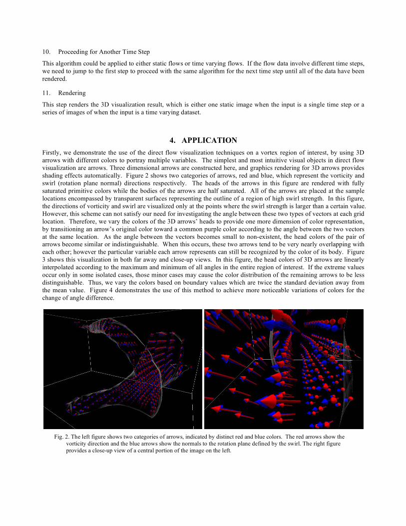
4. APPLICATION Firstly, we demonstrate the use of the direct flow visualization techniques on a vortex region of interest, by using 3D arrows with different colors to portray multiple variables. The simplest and most intuitive visual objects in direct flow visualization are arrows. Three dimensional arrows are constructed here, and graphics rendering for 3D arrows provides shading effects automatically. Figure 2 shows two categories of arrows, red and blue, which represent the vorticity and swirl (rotation plane normal) directions respectively. The heads of the arrows in this figure are rendered with fully saturated primitive colors while the bodies of the arrows are half saturated. All of the arrows are placed at the sample locations encompassed by transparent surfaces representing the outline of a region of high swirl strength. In this figure, the directions of vorticity and swirl are visualized only at the points where the swirl strength is larger than a certain value. However, this scheme can not satisfy our need for investigating the angle between these two types of vectors at each grid location. Therefore, we vary the colors of the 3D arrows’ heads to provide one more dimension of color representation, by transitioning an arrow’s original color toward a common purple color according to the angle between the two vectors at the same location. As the angle between the vectors becomes small to non-existent, the head colors of the pair of arrows become similar or indistinguishable. When this occurs, these two arrows tend to be very nearly overlapping with each other; however the particular variable each arrow represents can still be recognized by the color of its body. Figure 3 shows this visualization in both far away and close-up views. In this figure, the head colors of 3D arrows are linearly interpolated according to the maximum and minimum of all angles in the entire region of interest. If the extreme values occur only in some isolated cases, those minor cases may cause the color distribution of the remaining arrows to be less distinguishable. Thus, we vary the colors based on boundary values which are twice the standard deviation away from the mean value. Figure 4 demonstrates the use of this method to achieve more noticeable variations of colors for the change of angle difference.

Fig. 2. The left figure shows two categories of arrows, indicated by distinct red and blue colors. The red arrows show the

vorticity direction and the blue arrows show the normals to the rotation plane defined by the swirl. The right figure provides a close-up view of a central portion of the image on the left.

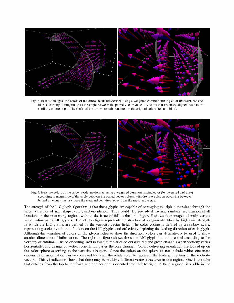
Fig. 3. In these images, the colors of the arrow heads are defined using a weighted common mixing color (between red and

blue) according to magnitude of the angle between the paired vector values. Vectors that are more aligned have more similarly colored tips. The shafts of the arrows remain rendered in the original colors (red and blue).

Fig. 4. Here the colors of the arrow heads are defined using a weighted common mixing color (between red and blue)

according to magnitude of the angle between the paired vector values, with the interpolation occurring between boundary values that are twice the standard deviation away from the mean angle size.

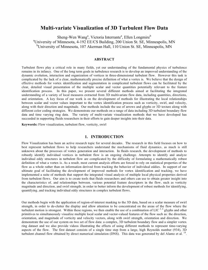
The strength of the LIC glyph algorithm is that these glyphs are capable of conveying multiple dimensions through the visual variables of size, shape, color, and orientation. They could also provide dense and random visualization at all locations in the interesting regions without the issue of full occlusion. Figure 5 shows four images of multi-variate visualization using LIC glyphs. The left top figure represents the structure of a region identified by high swirl strength in which the LIC glyphs are defined by the vorticity vector field. The color coding is defined by a rainbow scale, representing a clear variation of colors on the LIC glyphs, and effectively depicting the leading direction of each glyph. Although this variation of colors on the glyphs helps to show the direction, colors can alternatively be used to show another dimension of information. The right top figure shows the same LIC glyphs but color coded according to the vorticity orientation. The color coding used in this figure varies colors with red and green channels when vorticity varies horizontally, and change of vertical orientation varies the blue channel. Colors delivering orientation are looked up on the color sphere according to the vorticity direction. Since the colors on the sphere do not include white, one more dimension of information can be conveyed by using the white color to represent the leading direction of the vorticity vectors. This visualization shows that there may be multiple different vortex structures in this region. One is the tube that extends from the top to the front, and another one is oriented from left to right. A third segment is visible in the

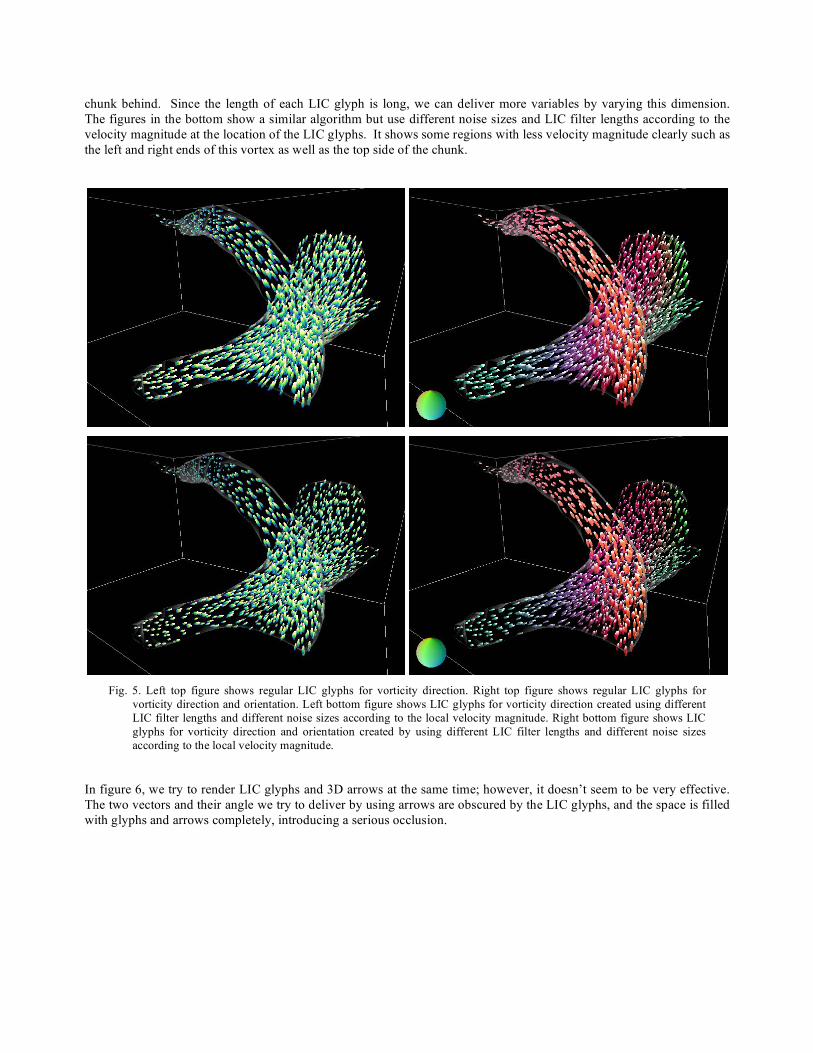
chunk behind. Since the length of each LIC glyph is long, we can deliver more variables by varying this dimension. The figures in the bottom show a similar algorithm but use different noise sizes and LIC filter lengths according to the velocity magnitude at the location of the LIC glyphs. It shows some regions with less velocity magnitude clearly such as the left and right ends of this vortex as well as the top side of the chunk.

Fig. 5. Left top figure shows regular LIC glyphs for vorticity direction. Right top figure shows regular LIC glyphs for

vorticity direction and orientation. Left bottom figure shows LIC glyphs for vorticity direction created using different LIC filter lengths and different noise sizes according to the local velocity magnitude. Right bottom figure shows LIC glyphs for vorticity direction and orientation created by using different LIC filter lengths and different noise sizes according to the local velocity magnitude.

In figure 6, we try to render LIC glyphs and 3D arrows at the same time; however, it doesn’t seem to be very effective. The two vectors and their angle we try to deliver by using arrows are obscured by the LIC glyphs, and the space is filled with glyphs and arrows completely, introducing a serious occlusion.

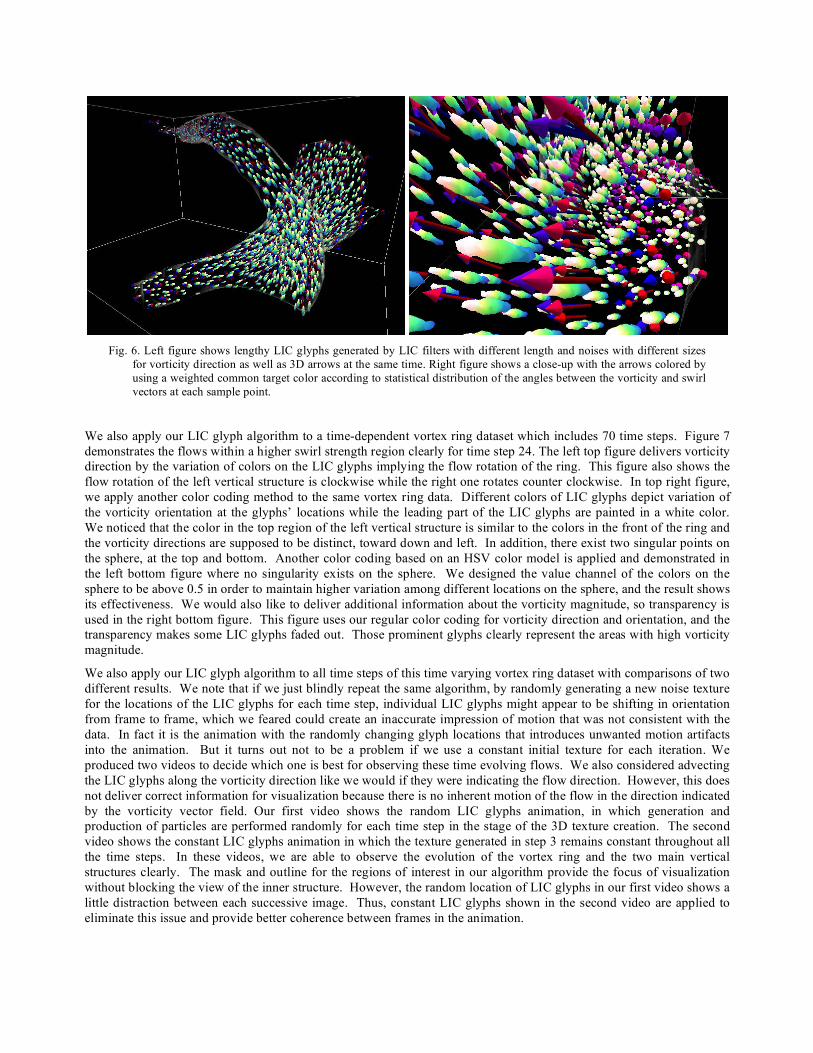
Fig. 6. Left figure shows lengthy LIC glyphs generated by LIC filters with different length and noises with different sizes

for vorticity direction as well as 3D arrows at the same time. Right figure shows a close-up with the arrows colored by using a weighted common target color according to statistical distribution of the angles between the vorticity and swirl vectors at each sample point.

We also apply our LIC glyph algorithm to a time-dependent vortex ring dataset which includes 70 time steps. Figure 7 demonstrates the flows within a higher swirl strength region clearly for time step 24. The left top figure delivers vorticity direction by the variation of colors on the LIC glyphs implying the flow rotation of the ring. This figure also shows the flow rotation of the left vertical structure is clockwise while the right one rotates counter clockwise. In top right figure, we apply another color coding method to the same vortex ring data. Different colors of LIC glyphs depict variation of the vorticity orientation at the glyphs’ locations while the leading part of the LIC glyphs are painted in a white color. We noticed that the color in the top region of the left vertical structure is similar to the colors in the front of the ring and the vorticity directions are supposed to be distinct, toward down and left. In addition, there exist two singular points on the sphere, at the top and bottom. Another color coding based on an HSV color model is applied and demonstrated in the left bottom figure where no singularity exists on the sphere. We designed the value channel of the colors on the sphere to be above 0.5 in order to maintain higher variation among different locations on the sphere, and the result shows its effectiveness. We would also like to deliver additional information about the vorticity magnitude, so transparency is used in the right bottom figure. This figure uses our regular color coding for vorticity direction and orientation, and the transparency makes some LIC glyphs faded out. Those prominent glyphs clearly represent the areas with high vorticity magnitude.

We also apply our LIC glyph algorithm to all time steps of this time varying vortex ring dataset with comparisons of two different results. We note that if we just blindly repeat the same algorithm, by randomly generating a new noise texture for the locations of the LIC glyphs for each time step, individual LIC glyphs might appear to be shifting in orientation from frame to frame, which we feared could create an inaccurate impression of motion that was not consistent with the data. In fact it is the animation with the randomly changing glyph locations that introduces unwanted motion artifacts into the animation. But it turns out not to be a problem if we use a constant initial texture for each iteration. We produced two videos to decide which one is best for observing these time evolving flows. We also considered advecting the LIC glyphs along the vorticity direction like we would if they were indicating the flow direction. However, this does not deliver correct information for visualization because there is no inherent motion of the flow in the direction indicated by the vorticity vector field. Our first video shows the random LIC glyphs animation, in which generation and production of particles are performed randomly for each time step in the stage of the 3D texture creation. The second video shows the constant LIC glyphs animation in which the texture generated in step 3 remains constant throughout all the time steps. In these videos, we are able to observe the evolution of the vortex ring and the two main vertical structures clearly. The mask and outline for the regions of interest in our algorithm provide the focus of visualization without blocking the view of the inner structure. However, the random location of LIC glyphs in our first video shows a little distraction between each successive image. Thus, constant LIC glyphs shown in the second video are applied to eliminate this issue and provide better coherence between frames in the animation.

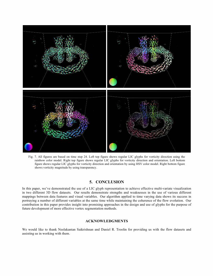
Fig. 7. All figures are based on time step 24. Left top figure shows regular LIC glyphs for vorticity direction using the

rainbow color model. Right top figure shows regular LIC glyphs for vorticity direction and orientation. Left bottom figure shows regular LIC glyphs for vorticity direction and orientation by using HSV color model. Right bottom figure shows vorticity magnitude by using transparency.

5. CONCLUSION In this paper, we’ve demonstrated the use of a LIC glyph representation to achieve effective multi-variate visualization in two different 3D flow datasets. Our results demonstrate strengths and weaknesses in the use of various different mappings between data features and visual variables. Our algorithm applied to time varying data shows its success in portraying a number of different variables at the same time while maintaining the coherence of the flow evolution. Our contribution in this paper provides insight into promising approaches in the design and use of glyphs for the purpose of future development of more effective vortex segmentation methods.

ACKNOWLEDGMENTS

We would like to thank Neelakantan Saikrishnan and Daniel R. Troolin for providing us with the flow datasets and assisting us in working with them.

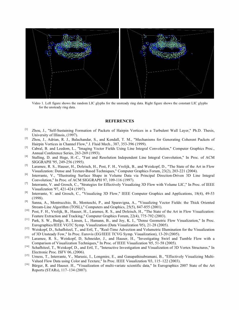
Video 1. Left figure shows the random LIC glyphs for the unsteady ring data. Right figure shows the constant LIC glyphs

for the unsteady ring data.

REFERENCES

[1] Zhou, J., "Self-Sustaining Formation of Packets of Hairpin Vortices in a Turbulent Wall Layer," Ph.D. Thesis, University of Illinois, (1997).

[2] Zhou, J., Adrian, R. J., Balachandar, S., and Kendall, T. M., "Mechanisms for Generating Coherent Packets of Hairpin Vortices in Channel Flow," J. Fluid Mech., 387, 353-396 (1999).

[3] Cabral, B. and Leedom, L., "Imaging Vector Fields Using Line Integral Convolution," Computer Graphics Proc., Annual Conference Series, 263-269 (1993).

[4] Stalling, D. and Hege, H.-C., "Fast and Resolution Independent Line Integral Convolution," In Proc. of ACM SIGGRAPH '95, 249-256 (1995).

[5] Laramee, R. S., Hauser, H., Doleisch, H., Post, F. H., Vrolijk, B., and Weiskopf, D., "The State of the Art in Flow Visualization: Dense and Texture-Based Techniques," Computer Graphics Forum, 23(2), 203-221 (2004).

[6] Interrante, V., "Illustrating Surface Shape in Volume Data via Principal Direction-Driven 3D Line Integral Convolution," In Proc. of ACM SIGGRAPH 97, 109-116 (1997).

[7] Interrante, V. and Grosch, C., "Strategies for Effectively Visualizing 3D Flow with Volume LIC," In Proc. of IEEE Visualization '97, 421-424 (1997).

[8] Interrante, V. and Grosch, C., "Visualizing 3D Flow," IEEE Computer Graphics and Applications, 18(4), 49-53 (1998).

[9] Sanna, A., Montrucchio, B., Montuschi, P., and Sparavigna, A., "Visualizing Vector Fields: the Thick Oriented Stream-Line Algorithm (TOSL)," Computers and Graphics, 25(5), 847-855 (2001).

[10] Post, F. H., Vrolijk, B., Hauser, H., Laramee, R. S., and Doleisch, H., "The State of the Art in Flow Visualization: Feature Extraction and Tracking," Computer Graphics Forum, 22(4), 775-792 (2003).

[11] Park, S. W., Budge, B., Linsen, L., Hamann, B., and Joy, K. I., "Dense Geometric Flow Visualization," In Proc. Eurographics/IEEE VGTC Symp. Visualization (Data Visualization '05), 21-28 (2005).

[12] Weiskopf, D., Schafhitzel, T., and Ertl, T., "Real-Time Advection and Volumetric Illumination for the Visualization of 3D Unsteady Fow," In Proc. Eurovis (EG/IEEE TCVG Symp. Visualization), 13-20 (2005).

[13] Laramee, R. S., Weiskopf, D, Schneider, J., and Hauser, H., "Investigating Swirl and Tumble Flow with a Comparison of Visualization Techniques," In Proc. of IEEE Visualization '05, 51-58 (2005).

[14] Schafhitzel, T., Weiskopf, D., and Ertl, T., "Interactive Investigation and Visualization of 3D Vortex Structures," In Electronic Proc. ISFV 06, (2006).

[15] Urness, T., Interrante, V., Marusic, I., Longmire, E., and Ganapathisubramani, B., "Effectively Visualizing Multi-Valued Flow Data using Color and Texture," In Proc. IEEE Visualization '03, 115–122 (2003).

[16] Bürger, R. and Hauser. H., "Visualization of multi-variate scientific data," In Eurographics 2007 State of the Art Reports (STARs), 117–134 (2007).

[17] Berdahl, C. H. and Thompson, D. S., "Education of Swirling Structure Using the Velocity Gradient Tensor," AIAA J., 28(8), 1347-1352 (1990).

[18] del Alamo, J. C., Jimenez, J., Zandonade, P., and Moser, R. D., "Scaling of the Energy Spectra of Turbulent Channels," J. Fluid Mech., 500, 135-144 (2004).

[19] Mallo, O., Peikert, R., Sigg, C. and Sadlo, F., "Illuminated Lines Revisited", In Proc. of IEEE Visualization '05, 19-26 (2005)

[20] Hall. P., "Volume Rendering of Vector Fields," The Visual Computer, 10(2), 69–78 (1993). [21] Jankun-Kelly, M., Jiang, M., Thompson, D., and Machiraju, R., "Vortex Visualization for Practical Engineering

Applications," IEEE Transactions on Visualization and Computer Graphics, 12(5), 957-964 (2006). [22] Troolin, D. R. and Longmire, E. K., "Volumetric Velocity Measurements of Vortex Rings from Inclined Exits,"

Experiments in Fluids, (2009). [23] Loffelmann, H. and Groller E., "Enhancing the Visualization of Characteristic Structures in Dynamical Systems," In

EG Workshop on Visualization in Scientific Computing, 59-68 (1998).