Multiattribute judgements under uncertainty : a conjoint - Ideals

UNIVERSITY OFILLINOIS LIBRARY

AT URBANA-CHAMPAIGNBOOKSTACKS

Digitized by the Internet Archive

in 2011 with funding from

University of Illinois Urbana-Champaign

http://www.archive.org/details/multiattributeju1564basu

BEBRFACULTY WORKINGPAPER NO. 89-1564

Multiattribute JudgmentsUnder Uncertainty: A Conjoint

Measurement Approach

| I I M ( ^ tf\Q(

>«>ll t Uh ILUlMUiSU^BANA-CHAMPAIGN

Amiya K. Basil

Manoj Hastak

College of Commerce and Business Administration

Bureau of Economic and Business Research

University of Illinois Urbana-Champaign

BEBR

FACULTY WORKING PAPER NO. 89-1564

College of Commerce and Business Administration

University of Illinois at Urbana- Champaign

May 1989

Multiattribute Judgments Under Uncertainty:A Conjoint Measurement Approach

Amiya K. Basu, ProfessorDepartment of Business Administration

Manoj Hastak, Assistant ProfessorDepartment of Business Administration

MULTIATTRIBUTE JUDGMENTS UNDER UNCERTAINTY :

A CONJOINT MEASUREMENT APPROACH

Abstract

A methodology to predict product choice under uncertainty in attribute values is proposed

and tested. The methodology consists of (i) estimating the multiattribute utility function of

a consumer, and (ii) predicting new product evaluation based on expected utility computed

using the estimated utility function. To test the methodology, conjoint analysis is used to

estimate a respondent's multiattribute utility function. Next, the respondent is asked to

evaluate hypothetical product profiles with uncertain attribute values. The observed evalu-

ations are compared with predictions using the proposed technique and also a naive model

which ignores attribute uncertainty. In the sample studied, both the proposed technique

and the naive model predicted reasonably well, but neither model performed significantly

better than the other.

INTRODUCTION

Multiattribute modeling of consumer choice is a well known paradigm in marketing re-

search. The model rests on the assumption that consumers perceive a product as a 'profile'

or combination of attribute values. For example, a television set may be perceived as a

combination of its picture quality, longevity, audio quality, etc. The consumer is assumed

to integrate information about different attribute values to form an overall evaluation (or

assess utility) for each alternative, and to choose the one that maximizes utility subject to

budget constraints. Utility is clearly a function of the individual attribute values.

The multiattribute approach to choice modeling has enjoyed considerable popularity in the

marketing literature. Significant progress has been made in the last twenty years toward the

determination of the form and parameters of multiattribute utility functions (see Shocker

and Srinivasan 1979, Green and Srinivasan 1978, Wilkie and Pessemier 1973, Anderson

1974). One commonly used and widely accepted model to emerge from this research is the

additive conjoint measurement model. The model can be briefly described as follows :

Let (xi, £2, • • • > Xn) represent the vector of attribute values for a product with n significant

attributes. Then, the overall utility function for the product can be expressed as

n

(1) U{xu x2 ,...,xn )= ^Ui{xi)

»=i

where C/» is the part-worth utility function for attribute i.

Data for the model can be collected through either the 'full profile' or 'pairwise trade-off'

methods. In the 'full profile' approach, the consumer is asked to rate or rank order a

large number of hypothetical 'product profiles'. These profiles are generated by creating

combinations of attribute values across all significant attributes. Parameters of the part

worth utility functions are derived from ratings or rank orders provided by the subjects.

Once these parameters are available, it is possible to determine the utility of a consumer

for any given combination of attribute values, and hence predict whether the consumer will

choose the product over other alternatives. This predictive feature of the model makes it

particularly relevant for managerial application and use.

RESEARCH ISSUES

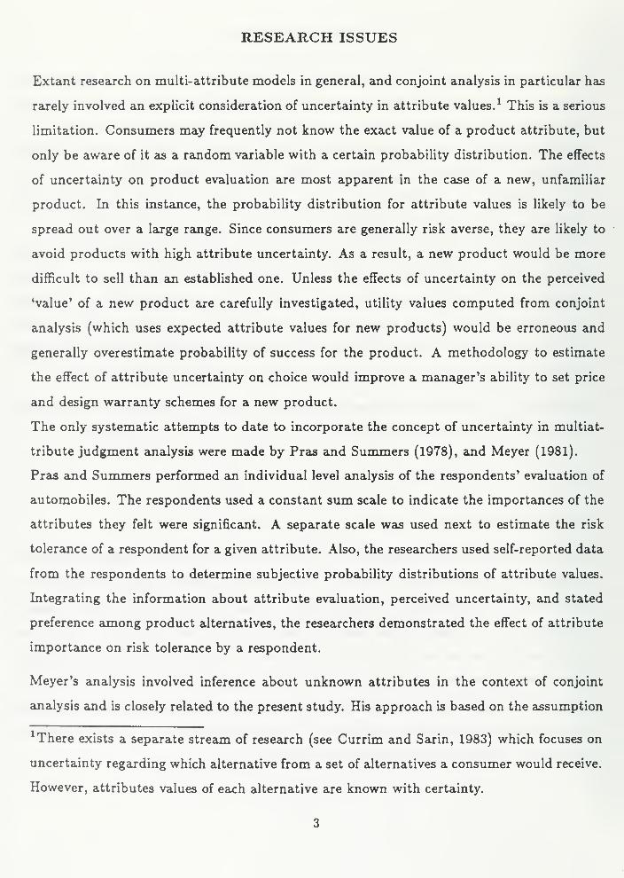
Extant research on multi-attribute models in general, and conjoint analysis in particular has

rarely involved an explicit consideration of uncertainty in attribute values. 1 This is a serious

limitation. Consumers may frequently not know the exact value of a product attribute, but

only be aware of it as a random variable with a certain probability distribution. The effects

of uncertainty on product evaluation are most apparent in the case of a new, unfamiliar

product. In this instance, the probability distribution for attribute values is likely to be

spread out over a large range. Since consumers are generally risk averse, they are likely to

avoid products with high attribute uncertainty. As a result, a new product would be more

difficult to sell than an established one. Unless the effects of uncertainty on the perceived

'value' of a new product are carefully investigated, utility values computed from conjoint

analysis (which uses expected attribute values for new products) would be erroneous and

generally overestimate probability of success for the product. A methodology to estimate

the effect of attribute uncertainty on choice would improve a manager's ability to set price

and design warranty schemes for a new product.

The only systematic attempts to date to incorporate the concept of uncertainty in multiat-

tribute judgment analysis were made by Pras and Summers (1978), and Meyer (1981).

Pras and Summers performed an individual level analysis of the respondents' evaluation of

automobiles. The respondents used a constant sum scale to indicate the importances of the

attributes they felt were significant. A separate scale was used next to estimate the risk

tolerance of a respondent for a given attribute. Also, the researchers used self-reported data

from the respondents to determine subjective probability distributions of attribute values.

Integrating the information about attribute evaluation, perceived uncertainty, and stated

preference among product alternatives, the researchers demonstrated the effect of attribute

importance on risk tolerance by a respondent.

Meyer's analysis involved inference about unknown attributes in the context of conjoint

analysis and is closely related to the present study. His approach is based on the assumption

There exists a separate stream of research (see Currim and Sarin, 1983) which focuses on

uncertainty regarding which alternative from a set of alternatives a consumer would receive.

However, attributes values of each alternative are known with certainty.

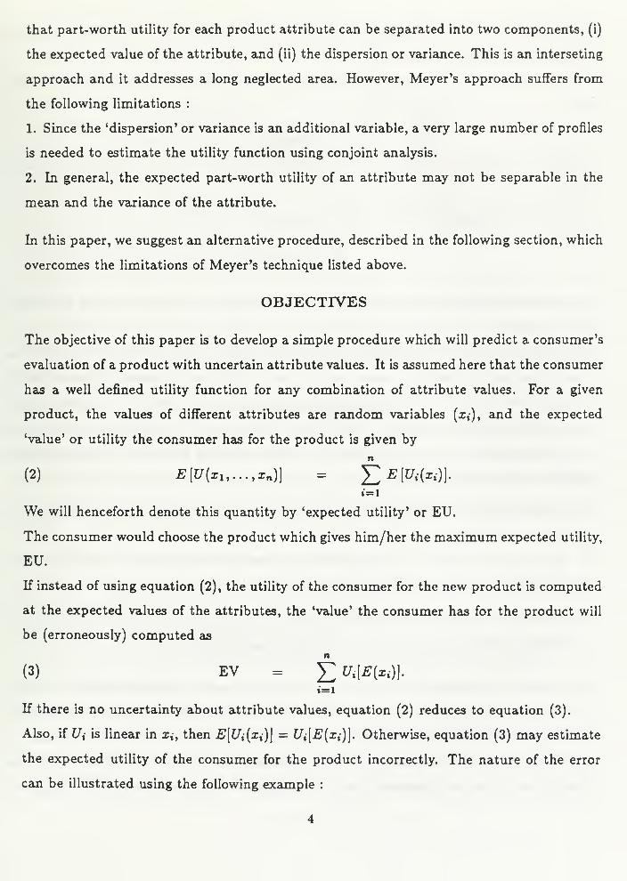
that part-worth utility for each product attribute can be separated into two components, (i)

the expected value of the attribute, and (ii) the dispersion or variance. This is an interseting

approach and it addresses a long neglected area. However, Meyer's approach suffers from

the following limitations :

1. Since the 'dispersion' or variance is an additional variable, a very large number of profiles

is needed to estimate the utility function using conjoint analysis.

2. In general, the expected part-worth utility of an attribute may not be separable in the

mean and the variance of the attribute.

In this paper, we suggest an alternative procedure, described in the following section, which

overcomes the limitations of Meyer's technique listed above.

OBJECTIVES

The objective of this paper is to develop a simple procedure which will predict a consumer's

evaluation of a product with uncertain attribute values. It is assumed here that the consumer

has a well defined utility function for any combination of attribute values. For a given

product, the values of different attributes are random variables (x t ), and the expected

'value' or utility the consumer has for the product is given by

n

(2) E[U(zu ...,xn)] = ^2E[Ui(xi)\.t=i

We will henceforth denote this quantity by 'expected utility' or EU.

The consumer would choose the product which gives him/her the maximum expected utility,

EU.

If instead of using equation (2), the utility of the consumer for the new product is computed

at the expected values of the attributes, the 'value' the consumer has for the product will

be (erroneously) computed as

n

(3) EV = £ tf,-[£?(*,-)].

t=i

If there is no uncertainty about attribute values, equation (2) reduces to equation (3).

Also, if U{ is linear in i t , then E[Ui(xi)\ = Ui[E(x{)\. Otherwise, equation (3) may estimate

the expected utility of the consumer for the product incorrectly. The nature of the error

can be illustrated using the following example :

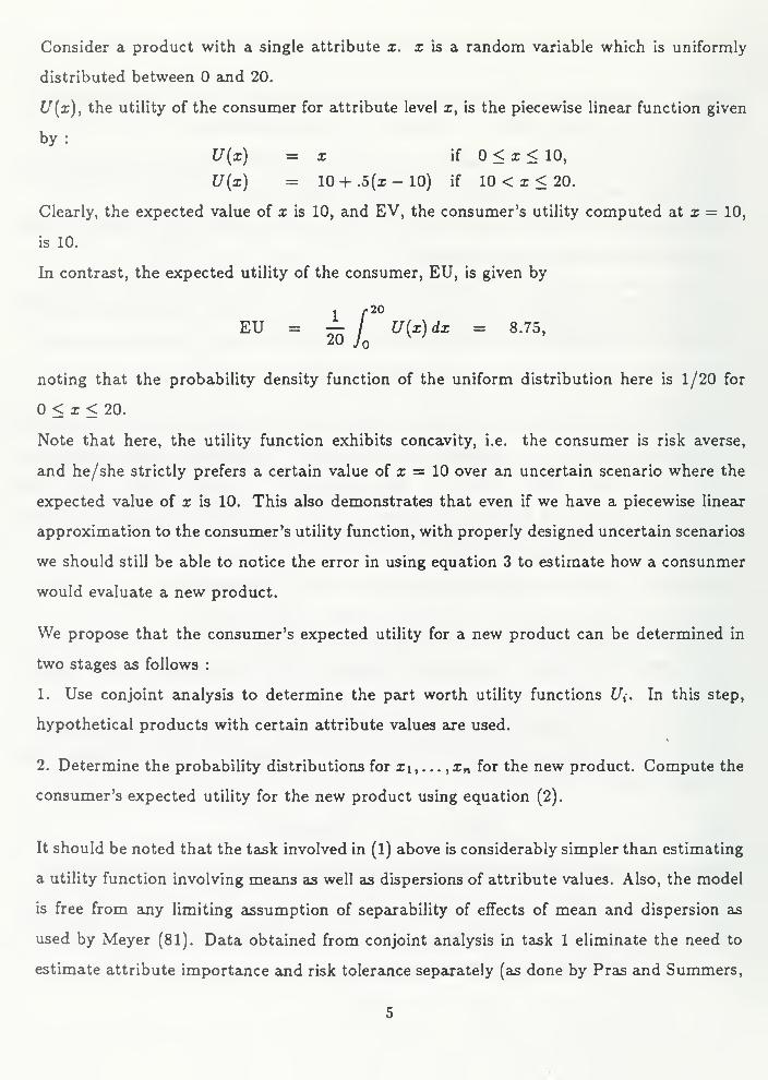
Consider a product with a single attribute x. x is a random variable which is uniformly

distributed between and 20.

U{x), the utility of the consumer for attribute level x, is the piecewise linear function given

by:U{x) = x if < x < 10,

U{x) = 10 + .5(x - 10) if 10 < x < 20.

Clearly, the expected value of x is 10, and EV, the consumer's utility computed at x = 10,

is 10.

In contrast, the expected utility of the consumer, EU, is given by

•20

EU = —/ U{x)dx = 8.75,

noting that the probability density function of the uniform distribution here is 1/20 for

< x < 20.

Note that here, the utility function exhibits concavity, i.e. the consumer is risk averse,

and he/she strictly prefers a certain value of x = 10 over an uncertain scenario where the

expected value of x is 10. This also demonstrates that even if we have a piecewise linear

approximation to the consumer's utility function, with properly designed uncertain scenarios

we should still be able to notice the error in using equation 3 to estimate how a consunmer

would evaluate a new product.

We propose that the consumer's expected utility for a new product can be determined in

two stages as follows :

1. Use conjoint analysis to determine the part worth utility functions U{. In this step,

hypothetical products with certain attribute values are used.

2. Determine the probability distributions for Xi, . . . ,xn for the new product. Compute the

consumer's expected utility for the new product using equation (2).

It should be noted that the task involved in (l) above is considerably simpler than estimating

a utility function involving means as well as dispersions of attribute values. Also, the model

is free from any limiting assumption of separability of effects of mean and dispersion as

used by Meyer (81). Data obtained from conjoint analysis in task 1 eliminate the need to

estimate attribute importance and risk tolerance separately (as done by Pras and Summers,

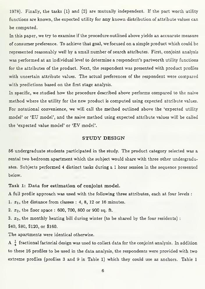
1978). Finally, the tasks (1) and (2) are mutually independent. If the part worth utility

functions are known, the expected utility for any known distribution of attribute values can

be computed.

In this paper, we try to examine if the procedure outlined above yields an accuarate measure

of consumer preference. To achieve that goal, we focused on a simple product which could be

represented reasonably well by a small number of search attributes. First, conjoint analysis

was performed at an individual level to determine a respondent's partworth utility functions

for the attributes of the product. Next, the respondent was presented with product profiles

with uncertain attribute values. The actual preferences of the respondent were compared

with predictions based on the first stage analysis.

In specific, we studied how the procedure described above performs compared to the naive

method where the utility for the new product is computed using expected attribute values.

For notational convenience, we will call the method outlined above the 'expected utility

model' or 'EU model', and the naive method using expected attribute values will be called

the 'expected value model' or 'EV model'.

STUDY DESIGN

56 undergraduate students participated in the study. The product category selected was a

rental two bedroom apartment which the subject would share with three other undergradu-

ates. Subjects performed 4 distinct tasks during a 1 hour session in the sequence presented

below.

Task 1: Data for estimation of conjoint model.

A full profile approach was used with the following three attributes, each at four levels :

1. xi, the distance from classes : 4, 8, 12 or 16 minutes.

2. x2 , the floor space : 600, 700, 800 or 900 sq. ft.

3. £3, the monthly heating bill during winter (to be shared by the four residents) :

$40, $80, $120, or $160.

The apartments were identical otherwise.

A 4 fractional factorial design was used to collect data for the conjoint analysis. In addition

to these 16 profiles to be used in the data analysis, the respondents were provided with two

extreme profiles (profiles 3 and 9 in Table 1) which they could use as anchors. Table 1

6

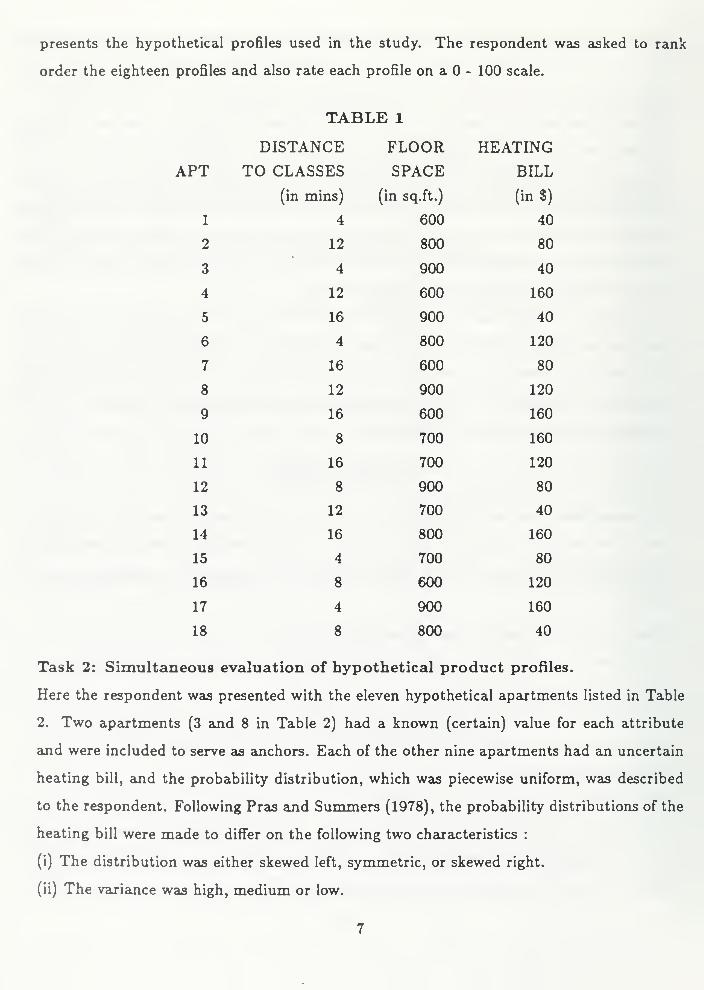
presents the hypothetical profiles used in the study. The respondent was asked to rank

order the eighteen profiles and also rate each profile on a - 100 scale.

TABLE 1

DISTANCE FLOOR HEATING

PT TO CLASSES SPACE BILL

(in mins) (in sq.ft.) (in$)

1 4 600 40

2 12 800 80

3 4 900 40

4 12 600 160

5 16 900 40

6 4 800 120

7 16 600 80

8 12 900 120

9 16 600 160

10 8 700 160

11 16 700 120

12 8 900 80

13 12 700 40

14 16 800 160

15 4 700 80

16 8 600 120

17 4 900 160

18 8 800 40

Task 2: Simultaneous evaluation of hypothetical product profiles.

Here the respondent was presented with the eleven hypothetical apartments listed in Table

2. Two apartments (3 and 8 in Table 2) had a known (certain) value for each attribute

and were included to serve as anchors. Each of the other nine apartments had an uncertain

heating bill, and the probability distribution, which was piecewise uniform, was described

to the respondent. Following Pras and Summers (1978), the probability distributions of the

heating bill were made to differ on the following two characteristics :

(i) The distribution was either skewed left, symmetric, or skewed right,

(ii) The variance was high, medium or low.

These nine profiles consisted of the (3 X 3) combinations of the three levels of these two

characteristics. The other two attributes were known with certainty, and their values were

randomly varied from profile to profile. The respondent rank ordered the 11 profiles and

also rated each profile on a - 100 scale.

Task 3: Pairwise comparison of hypothetical product profiles.

The respondent was presented with eight pairs of hypothetical apartments. Each pair con-

sisted of one apartment with known (certain) values for all attributes, and one apartment

with known (certain) values of distance and floor space, but uncertainty in heating bill. The

distance and floor space were the same for both members of a pair. The known (certain)

heating bill was always greater than or equal to the expected value of the uncertain heating

bill.2

The uncertain heating bills differed across pairs on the following characteristics :

(i) The variance was low, or high.

(ii) The distribution was symmmetric, or skewed right (the 'skewed left' case was omitted

due to time constraints).

(iii) The certain heating bill in the pair exceeded the expected value of the uncertain heating

bill by a small ($0 - $5) or a large ($10 - $20) amount.

The eight pairs consisted of (2 x 2 x 2) combinations of the two levels of the three attributes.

In four pairs the uncertain case was presented first, and in the other four the certain case

was presented first. For each pair, the respondent was asked to indicate on a five point scale

how strongly he/she preferred the second apartment in the pair over the first.3

Table 3 presents one pair of apartments used in the study.

Task 4: General information.

Finally, the respondent completed a short questionnaire which obtained background infor-

mation. It also contained a constant sum scale where the respondent was asked to divide

100 points among four attributes of an apartment : rent, distance from school, floor space

and heating bill, according to importance.

This was done since we felt that the respondent would have a negative utility for heating

bill.

3Note that for four pairs, the heating bill of the second apartment was uncertain, and in

the remaining four, it was known with certainty.

8

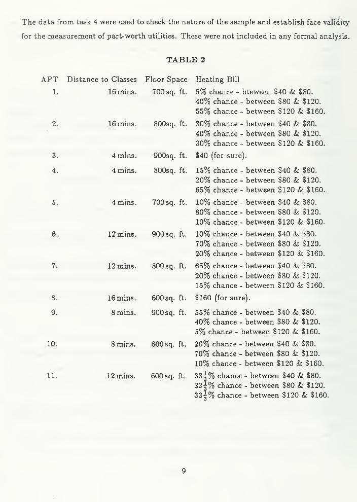
The data from task 4 were used to check the nature of the sample and establish face validity

for the measurement of part-worth utilities. These were not included in any formal analysis.

TABLE 2

APT Distance to Classes Floor Space

1. 16mins. 700 sq. ft.

2. 16mins. 800sq. ft.

3.

4.

5.

6.

7.

8.

9.

10.

11.

4mins.

4 mins.

4 mins.

12 mins.

16 mins.

8 mins.

8 mins.

12 mins.

900sq. ft.

800sq. ft.

700 sq. ft.

900 sq. ft.

12 mins. 800 sq. ft.

600 sq. ft.

900 sq. ft.

600 sq. ft.

600 sq. ft.

Heating Bill

5% chance -

40% chance -

55% chance -

30% chance -

40% chance -

30% chance -

$40 (for sure)

bteween $40 & $80.

• between $80 & $120.

between $120 & $160.

between $40 & $80.

• between $80 & $120.

• between $120 & $160.

15% chance - between












$160 (for sure).

$40 & $80.

$80 & $120.

$120 & $160.

$40 & $80.

$80 & $120.

$120 & $160.

$40 & $80.

$80 & $120.

$120 & $160.

$40 & $80.

$80 & $120.

$120 & $160.

55% chance - between $40 & $80.





10% chance - between $120 k $160.

33^% chance - between $40 & $80.

33|% chance - between $80 & $120.

33|% chance - between $120 & $160.

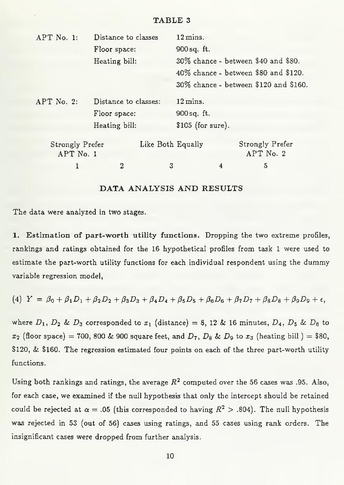
TABLE 3

APT No. 1: Distance to classes 12mins.

Floor space: 900 sq. ft.

Heating bill: 30% chance - between $40 and $80.

40% chance - between $80 and $120.

30% chance - between $120 and $160.

APT No. 2: Distance to classes: 12mins.

Floor space: 900 sq. ft.

Heating bill: $105 (for sure).

Strongly Prefer Like Both Equally Strongly Prefer

APT No. 1 APT No. 2

DATA ANALYSIS AND RESULTS

The data were analyzed in two stages.

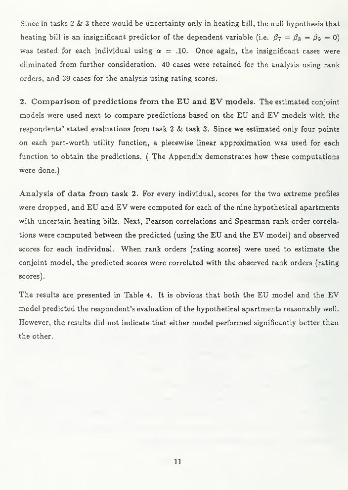
1. Estimation of part-worth utility functions. Dropping the two extreme profiles,

rankings and ratings obtained for the 16 hypothetical profiles from task 1 were used to

estimate the part-worth utility functions for each individual respondent using the dummy

variable regression model,

(4) Y = (3 + 1D l + foD2 + PzDz + P4D4 + 5D5 + (36D6 + 7D7 + psD8 + {39D9 + e,

where D\yD2 & D$ corresponded to x\ (distance) = 8, 12 & 16 minutes, D4, D5 & Dq to

x2 (floor space) = 700, 800 & 900 square feet, and D7 , D8 & Dg to x3 (heating bill ) = $80,

$120, & $160. The regression estimated four points on each of the three part-worth utility

functions.

Using both rankings and ratings, the average R 2 computed over the 56 cases was .95. Also,

for each case, we examined if the null hypothesis that only the intercept should be retained

could be rejected at a = .05 (this corresponded to having R 2 > .804). The null hypothesis

was rejected in 53 (out of 56) cases using ratings, and 55 cases using rank orders. The

insignificant cases were dropped from further analysis.

10

Since in tasks 2 & 3 there would be uncertainty only in heating bill, the null hypothesis that

heating bill is an insignificant predictor of the dependent variable (i.e. 07 = /?8 = fiQ = 0)

was tested for each individual using a = .10. Once again, the insignificant cases were

eliminated from further consideration. 40 cases were retained for the analysis using rank

orders, and 39 cases for the analysis using rating scores.

2. Comparison of predictions from the EU and EV models. The estimated conjoint

models were used next to compare predictions based on the EU and EV models with the

respondents' stated evaluations from task 2 & task 3. Since we estimated only four points

on each part-worth utility function, a piecewise linear approximation was used for each

function to obtain the predictions. ( The Appendix demonstrates how these computations

were done.)

Analysis of data from task 2. For every individual, scores for the two extreme profiles

were dropped, and EU and EV were computed for each of the nine hypothetical apartments

with uncertain heating bills. Next, Pearson correlations and Spearman rank order correla-

tions were computed between the predicted (using the EU and the EV model) and observed

scores for each individual. When rank orders (rating scores) were used to estimate the

conjoint model, the predicted scores were correlated with the observed rank orders (rating

scores).

The results are presented in Table 4. It is obvious that both the EU model and the EV

model predicted the respondent's evaluation of the hypothetical apartments reasonably well.

However, the results did not indicate that either model performed significantly better than

the other.

11

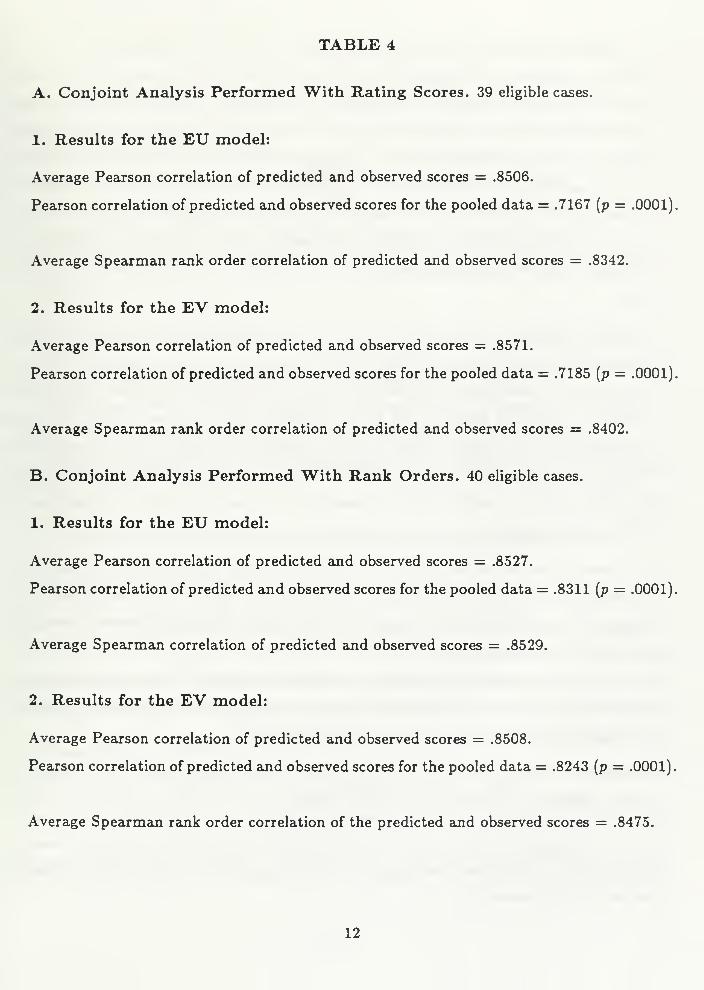
TABLE 4

A. Conjoint Analysis Performed With Rating Scores. 39 eligible cases.

1. Results for the EU model:

Average Pearson correlation of predicted and observed scores = .8506.

Pearson correlation of predicted and observed scores for the pooled data = .7167 (p = .0001).

Average Spearman rank order correlation of predicted and observed scores = .8342.

2. Results for the EV model:



Average Spearman rank order correlation of predicted and observed scores = .8402.

B. Conjoint Analysis Performed With Rank Orders. 40 eligible cases.




Average Spearman correlation of predicted and observed scores = .8529.




Average Spearman rank order correlation of the predicted and observed scores = .8475.

12

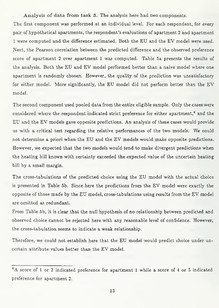
Analysis of data from task 3. The analysis here had two components.

The first component was performed at an individual level. For each respondent, for every

pair of hypothetical apartments, the respondent's evaluations of apartment 2 and apartment

1 were computed and the difference estimated. Both the EU and the EV model were used.

Next, the Pearson correlation between the predicted difference and the observed preference

score of apartment 2 over apartment 1 was computed. Table 5a presents the results of

the analysis. Both the EU and EV model performed better than a naive model where one

apartment is randomly chosen. However, the quality of the prediction was unsatisfactory

for either model. More significantly, the EU model did not perform better than the EV

model.

The second component used pooled data from the entire eligible sample. Only the cases were

considered where the respondent indicated strict preference for either apartment, 4 and the

EU and the EV models gave opposite predictions. An analysis of these cases would provide

us with a critical test regarding the relative performances of the two models. We could

not determine a priori when the EU and the EV models would make opposite predictions.

However, we expected that the two models would tend to make divergent predictions when

the heating bill known with certainty exceeded the expected value of the uncertain heating

bill by a small margin.

The cross-tabulations of the predicted choice using the EU model with the actual choice

is presented in Table 5b. Since here the predictions from the EV model were exactly the

opposite of those made by the EU model, cross-tabulations using results from the EV model

are omitted as redundant.

From Table 5b, it is clear that the null hypothesis of no relationship between predicted and

observed choice cannot be rejected here with any reasonable level of confidence. However,

the cross-tabulation seems to indicate a weak relationship.

Therefore, we could not establish here that the EU model would predict choice under un-

certain attribute values better than the EV model.

4A score of 1 or 2 indicated preference for apartment 1 while a score of 4 or 5 indicated

preference for apartment 2.

13

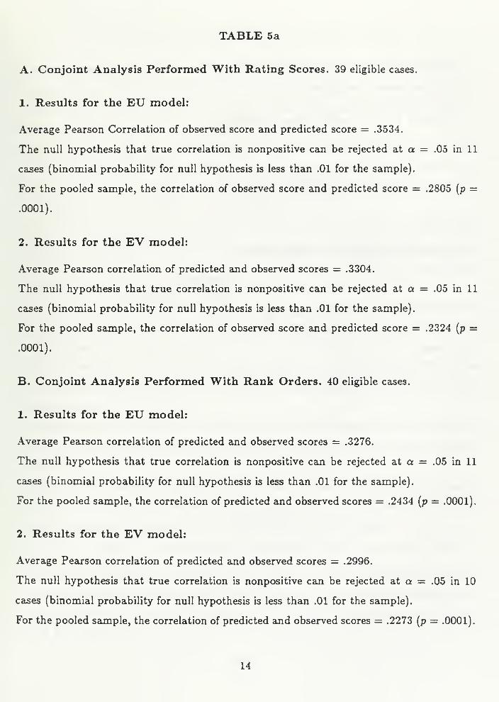
TABLE 5a

A. Conjoint Analysis Performed With Rating Scores. 39 eligible cases.


Average Pearson Correlation of observed score and predicted score = .3534.

The null hypothesis that true correlation is nonpositive can be rejected at a = .05 in 11

cases (binomial probability for null hypothesis is less than .01 for the sample).

For the pooled sample, the correlation of observed score and predicted score = .2805 (p =

.0001).





For the pooled sample, the correlation of observed score and predicted score = .2324 (p =

.0001).

B. Conjoint Analysis Performed With Rank Orders. 40 eligible cases.





For the pooled sample, the correlation of predicted and observed scores = .2434 (p = .0001).





For the pooled sample, the correlation of predicted and observed scores = .2273 (p = .0001).

14

TABLE 5b

Pooled Study of cases where the EU and EV models made opposite predictions and the

respondent had a clear choice.

A. Rating Scores Used. 63 cases (pooled).

Observed

APT 1. APT 2.

Predicted APT 1. 23 13

Using EU APT 2. 17 10

p = .940.

B. Rank Orders Used. 51 cases (pooled).

Observed

APT 1. APT 2.

Predicted APT 1. 20 9

Using EU APT 2. 14 8

p = .689.

15

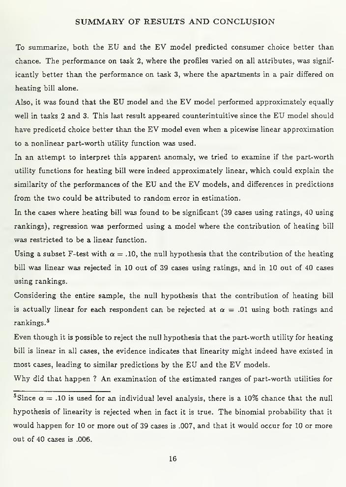
SUMMARY OF RESULTS AND CONCLUSION

To summarize, both the EU and the EV model predicted consumer choice better than

chance. The performance on task 2, where the profiles varied on all attributes, was signif-

icantly better than the performance on task 3, where the apartments in a pair differed on

heating bill alone.

Also, it was found that the EU model and the EV model performed approximately equally

well in tasks 2 and 3. This last result appeared counterintuitive since the EU model should

have predicetd choice better than the EV model even when a picewise linear approximation

to a nonlinear part-worth utility function was used.

In an attempt to interpret this apparent anomaly, we tried to examine if the part-worth

utility functions for heating bill were indeed approximately linear, which could explain the

similarity of the performances of the EU and the EV models, and differences in predictions

from the two could be attributed to random error in estimation.

In the cases where heating bill was found to be significant (39 cases using ratings, 40 using

rankings), regression was performed using a model where the contribution of heating bill

was restricted to be a linear function.

Using a subset F-test with a = .10, the null hypothesis that the contribution of the heating

bill was linear was rejected in 10 out of 39 cases using ratings, and in 10 out of 40 cases

using rankings.

Considering the entire sample, the null hypothesis that the contribution of heating bill

is actually linear for each respondent can be rejected at a = .01 using both ratings and

rankings. 5

Even though it is possible to reject the null hypothesis that the part-worth utility for heating

bill is linear in all cases, the evidence indicates that linearity might indeed have existed in

most cases, leading to similar predictions by the EU and the EV models.

Why did that happen ? An examination of the estimated ranges of part-worth utilities for

5 Since a = .10 is used for an individual level analysis, there is a 10% chance that the null

hypothesis of linearity is rejected when in fact it is true. The binomial probability that it

would happen for 10 or more out of 39 cases is .007, and that it would occur for 10 or more

out of 40 cases is .006.

16

distance, floor space and heating bill shows them to be approximately equally important

to the respondents on the average. However, an examination of information obtained from

task 4 indicates that rent is much more important than any of the three attributes included

in the study. This fact might have manifested itself as an approximately linear part-worth

utility function for heating bill.

Another reason might be the fact that the heating bill was to be shared by the four residents

of an apartment, thereby making the range of the heating bill to be paid by an individual

$10 - $40 rather than $40 - $160. The reduced range might have made the part-worth utility

function for heating bill approximately linear.

It is also possible that the respondents' perception of uncertainty in attribute values differed

from the uncertainty presnted in the questionnaire.

The reasons discussed so far indicate potential limitations of the study performed rather

than a failure of the technique proposed. Although these limitations could not be known

a priori, it is possible that a future study using an attribute which clearly has a nonlinear

part-worth utility function may establish the relative superiority of the EU model.

Finally, it is possible that the lack of success of the EU model here arises from a deeper

source, that the estimation of the conjoint model will give us part-worth utilities which will

no longer hold when attributes are not known with certainty. Previous research (Wittink,

Weinberg & Currim 1981, Wittink, Krishnamurthy & Nutter 1982) has already revealed the

fact that the estimated importance of an attribute would depend on the number of levels

of the attribute used in the conjoint analysis.Similarly, the presence of uncertainty might

affect evaluation by a consumer, and the expected utility given by equation (2) would no

longer be valid. Future research should address this question which is of crucial importance

to any attempt to incorporate uncertainty in attribute values into conjoint analysis.

17

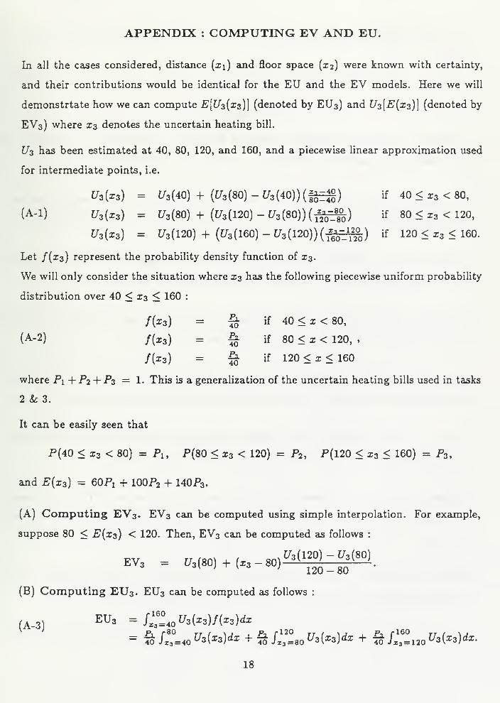
APPENDIX : COMPUTING EV AND EU.

In all the cases considered, distance (xi) and floor space (£2) were known with certainty,

and their contributions would be identical for the EU and the EV models. Here we will

demonstrtate how we can compute E[U3 (x3 )](denoted by EU3) and U3 [E(x3 )]

(denoted by

EV3) where 13 denotes the uncertain heating bill.

U3 has been estimated at 40, 80, 120, and 160, and a piecewise linear approximation used

for intermediate points, i.e.

U3 (x3 ) = U3 (40) + (U3 (80) - U3 (40)) (fj=g) if 40 < x3 < 80,

(A-l) U3 {xz ) = U3 (80) + (U3 (120)-U3 {80))(f^) if 80 < x3 < 120,

U3 {x3 ) = ^3(120) + (17,(160) -U8(120))(Jgg^) if 120<x3 <160.

Let /(X3) represent the probability density function of X3.

We will only consider the situation where x3 has the following piecewise uniform probability

distribution over 40 < x3 < 160 :

f{x3 ) = £ if 40<x<80,(A-2) f(X3 ) = % if 80 < x < 120, ,

/fca) = § if 120 < x < 160

where P\+ P2 + P3 = 1. This is a generalization of the uncertain heating bills used in tasks

2 & 3.

It can be easily seen that

P(40 < x3 < 80) = Pu P(80 < x3 < 120) = P2 , P(120 < x3 < 160) = P3 ,

and E{x3 ) = 60Pi + 100P2 + 140P3 .

(A) Computing EV3. EV3 can be computed using simple interpolation. For example,

suppose 80 < E(x3 ) < 120. Then, EV3 can be computed as follows :

EV3 = ^(80)^X3-80)^^:^ .

(B) Computing EU3 . EU3 can be computed as follows :

(A3)EU3 =H™A0 U3 {x3)f{x3 )dx

= ^C=40^(x3 )cfx + % SHl S0U3 (x3)dx + %C=120 U3 (x3 )dx.

18

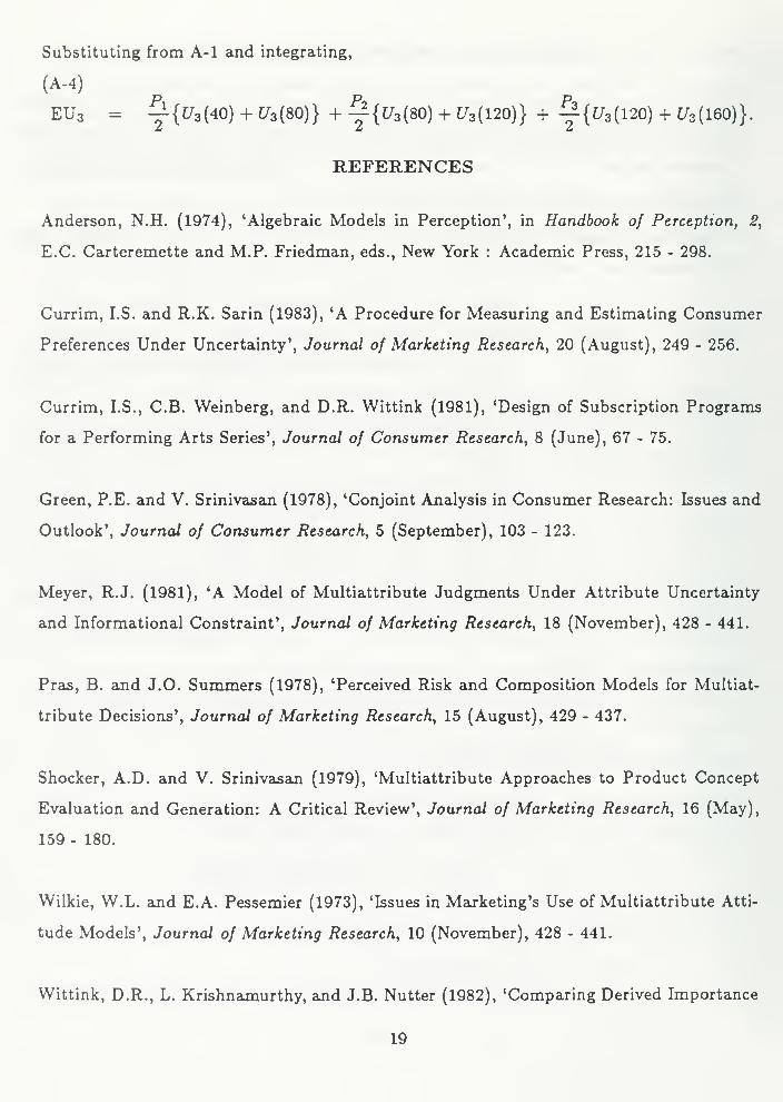
Substituting from A-l and integrating,

(A-4)

EU3 = y(C/3 (40) + U3 (S0)} + y {*73 (80) + CT3 (120)} + ^-{U3 {120) + ^3 (160)}.

REFERENCES

Anderson, N.H. (1974), 'Algebraic Models in Perception', in Handbook of Perception, 2,

E.C. Carteremette and M.P. Friedman, eds., New York : Academic Press, 215 - 298.

Currim, I.S. and R.K. Sarin (1983), 'A Procedure for Measuring and Estimating Consumer

Preferences Under Uncertainty', Journal of Marketing Research, 20 (August), 249 - 256.

Currim, I.S., C.B. Weinberg, and D.R. Wittink (1981), 'Design of Subscription Programs

for a Performing Arts Series', Journal of Consumer Research, 8 (June), 67 - 75.

Green, P.E. and V. Srinivasan (1978), 'Conjoint Analysis in Consumer Research: Issues and

Outlook', Journal of Consumer Research, 5 (September), 103 - 123.

Meyer, R.J. (1981), 'A Model of Multiattribute Judgments Under Attribute Uncertainty

and Informational Constraint', Journal of Marketing Research, 18 (November), 428 - 441.

Pras, B. and J.O. Summers (1978), 'Perceived Risk and Composition Models for Multiat-

tribute Decisions', Journal of Marketing Research, 15 (August), 429 - 437.

Shocker, A.D. and V. Srinivasan (1979), 'Multiattribute Approaches to Product Concept

Evaluation and Generation: A Critical Review', Journal of Marketing Research, 16 (May),

159 - 180.

Wilkie, W.L. and E.A. Pessemier (1973), 'Issues in Marketing's Use of Multiattribute Atti-

tude Models', Journal of Marketing Research, 10 (November), 428 - 441.

Wittink, D.R., L. Krishnamurthy, and J.B. Nutter (1982), 'Comparing Derived Importance

19

Weights Across Attributes', Journal of Consumer Research, 8 (March), 471 - 474.

20

HECKMANMDERY INC.

JUN95><'-To.|W> NMANCHESTFR

Documents

Multiattribute judgements under uncertainty : a conjoint - Ideals