26 July 2001

Chapter 30 1

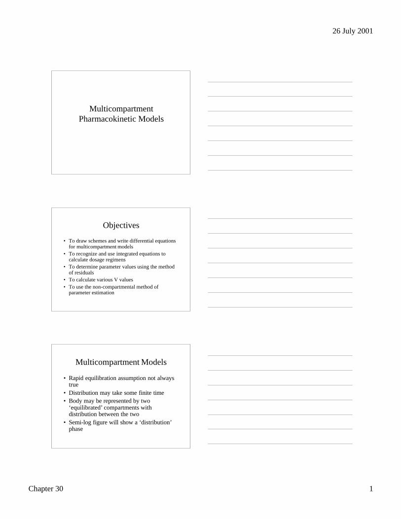
MulticompartmentPharmacokinetic Models

Objectives

• To draw schemes and write differential equationsfor multicompartment models

• To recognize and use integrated equations tocalculate dosage regimens

• To determine parameter values using the methodof residuals

• To calculate various V values• To use the non-compartmental method of

parameter estimation

Multicompartment Models

• Rapid equilibration assumption not alwaystrue

• Distribution may take some finite time• Body may be represented by two

‘equilibrated’ compartments withdistribution between the two

• Semi-log figure will show a ‘distribution’phase

26 July 2001

Chapter 30 2

One Compartment Model

Linear Plot

0

2

4

6

8

10

0 2 4 6 8 10 12 14 16 18 20 22 24

Con

cent

ratio

n (m

g/L)

Time (hr)

Cp = Cp0 • e-kel•t

Dose = 100 mg; V = 12.5 L; kel = 0.15 hr-1

One Compartment Model

Semi-log Plot

0.1

1

10

0 2 4 6 8 10 12 14 16 18 20 22 24

Con

cent

ratio

n (m

g/L)

Time (hr)

Cp = Cp0 • e-kel•t

Dose = 100 mg; V = 12.5 L; kel = 0.15 hr-1

Drug Disposition

Distribution• Commonly observed when early data are

collected• Deviation from a single exponential line• A rapid drop followed by a slower terminal

phase• Body can be represented by two (or more)

compartments

26 July 2001

Chapter 30 3

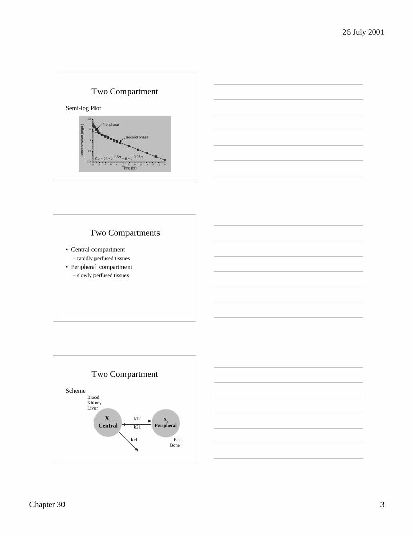
Two Compartment

Semi-log Plot

0.01

0.1

1

10

100

0 2 4 6 8 10 12 14 16 18 20 22 24

Con

cent

ratio

n (m

g/L)

Time (hr)

first phase

second phase

Cp = 24 • e-1.5•t + 6 • e-0.25•t

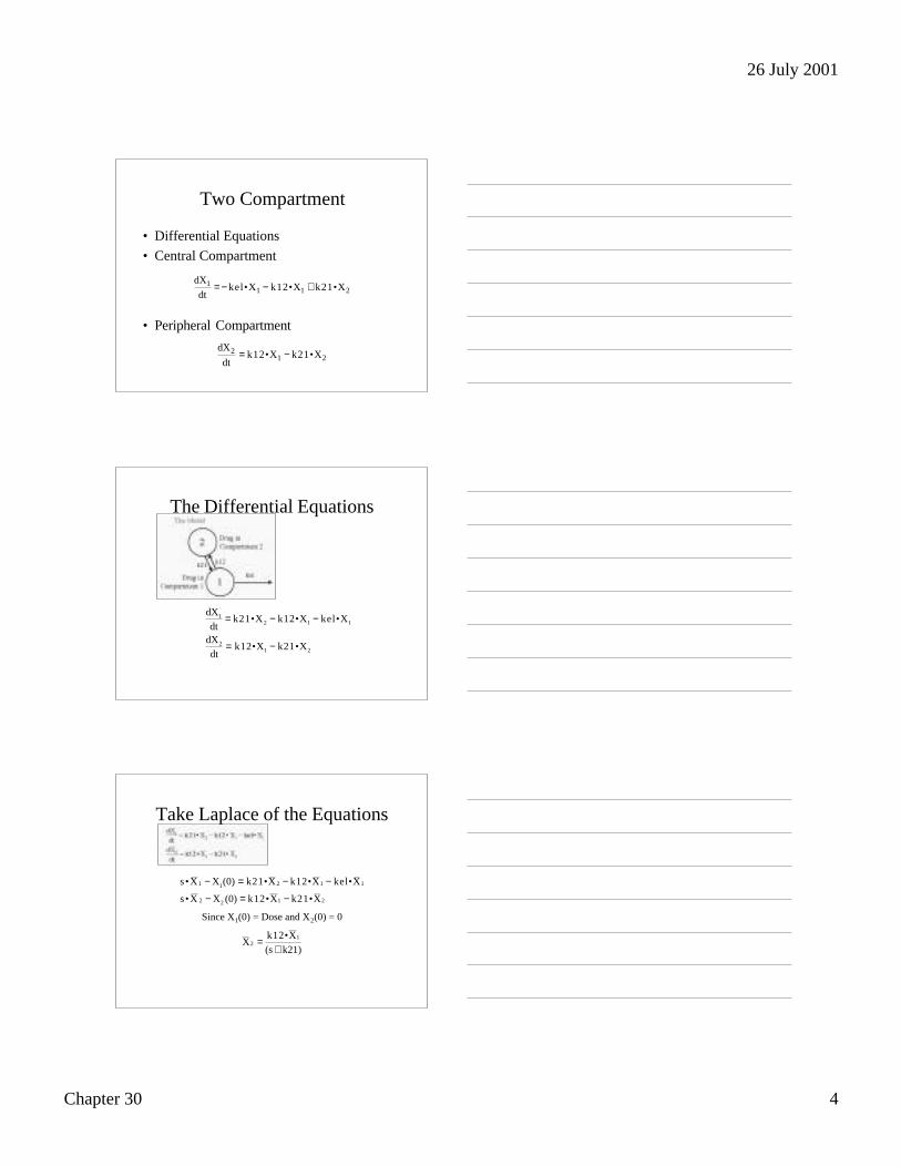
Two Compartments

• Central compartment– rapidly perfused tissues

• Peripheral compartment– slowly perfused tissues

Two Compartment

Scheme

X2

Peripheral

kel

k21

k12

BloodKidneyLiver

FatBone

X1

Central

26 July 2001

Chapter 30 4

Two Compartment

• Differential Equations

• Central Compartment

• Peripheral Compartment

dX1

dt= − kel•X1 − k12•X1 + k21•X2

dX2

dt= k12•X1 − k21•X2

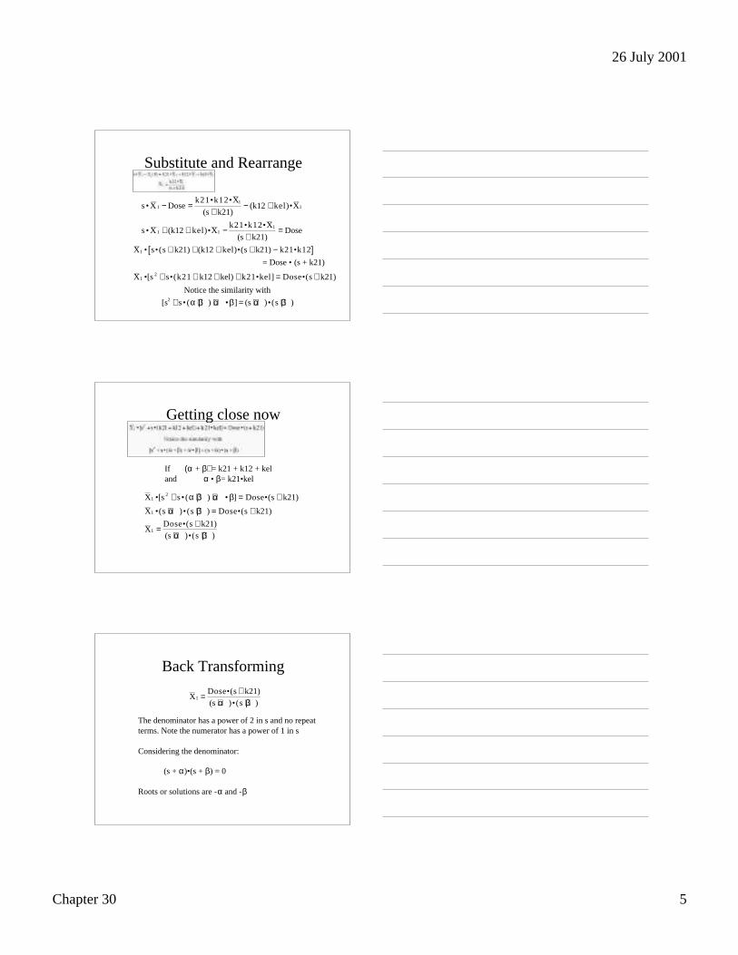
The Differential Equations

dX1

dt= k21•X2 − k12•X1 − kel•X1

dX2

dt= k12•X1 − k21•X2

Take Laplace of the Equations

s•X 1 − X1(0) = k21•X2 − k12•X1 − kel•X1

s•X 2 − X2 (0) = k12•X1 − k21•X2

Since X1(0) = Dose and X2(0) = 0

X2 = k12•X1

(s + k21)

26 July 2001

Chapter 30 5

Substitute and Rearrange

X1 • s•(s + k21) + (k12 + kel)•(s + k21) − k21•k12[ ]

X1 •[s 2 + s•(k21 + k12 + kel) + k21•kel] = Dose•(s + k21)

Notice the similarity with

[s2 + s • (α + β) +α •β] = (s +α)•(s +β)

s • X 1 − Dose =k21•k12•X1

(s + k21)− (k12 + kel)•X1

s • X 1 + (k12 + kel)•X1 − k21•k12•X1

(s + k21)= Dose

= Dose • (s + k21)

Getting close now

If (α + β) = k21 + k12 + keland α • β= k21•kel

X1 •[s 2 + s • (α + β ) +α • β] = Dose•(s + k21)

X1 •(s +α )•(s +β ) = Dose•(s + k21)

X1 = Dose•(s + k21)(s +α )•(s +β)

Back Transforming

The denominator has a power of 2 in s and no repeatterms. Note the numerator has a power of 1 in s

Considering the denominator:

(s + α)•(s + β) = 0

Roots or solutions are -α and -β

X1 = Dose•(s + k21)(s +α)•(s +β)

26 July 2001

Chapter 30 6

Dose•(s + k21)(s +α )•(s +β)

Root 1

First root is -α

Dose•(k21−α )

β − α( ) •e−α•t

X1 = Dose•(s + k21)(s +α)•(s +β)

Root 2

Second root is -β

•e−β•t

X1 = Dose•(s + k21)(s +α)•(s +β)

Dose•(k21−β)α − β( )

Dose•(s + k21)(s +α )•(s +β)

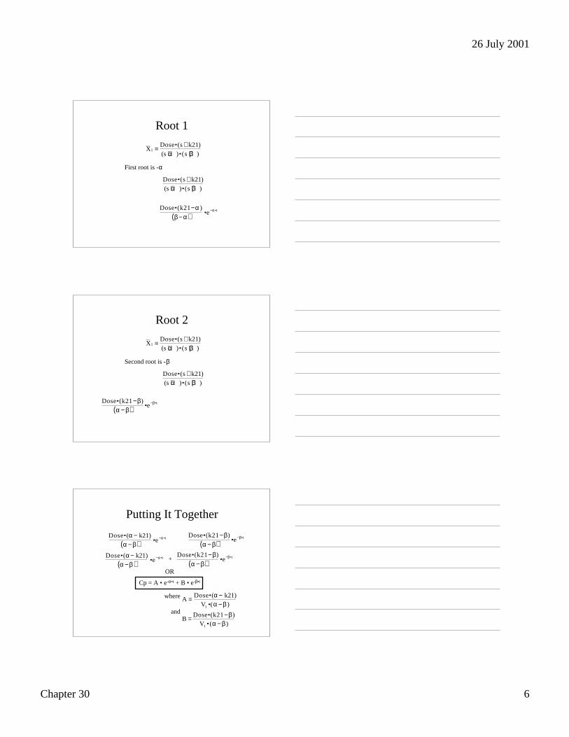
Putting It Together

OR

Dose•(α − k21)α − β( ) •e−α•t •e−β•tDose•(k21−β)

α − β( )Dose•(α− k21)

α − β( ) •e−α•t •e−β•tDose•(k21−β)

α − β( )+

Cp = A • e-α•t + B • e-β•t

where

and

A = Dose•(α − k21)V1 •(α − β )

B = Dose•(k21−β)V1 •(α − β )

26 July 2001

Chapter 30 7

Integrated Equation

Cp = A • e-α•t + B • e-β•t

α + β = kel + k12 + k21

α • β = kel•k21

α,β =α + β( ) ± α + β( )2 − 4• α • β

2or

α,β = kel + k12 + k21( ) ± kel + k12 + k21( )2 − 4•kel•k21

2

Parameter Determination

Method of Residuals• Parameters A, B, α and β can be determined

using the method of residuals• Since α > β (if α/β > 5)

– e-α•t approaches 0 quickly

• Terminal data points will be on a line

Method of Residuals

• Plotted on semi-log graph paper should give astraight line

• Calculate β from the terminal slope

Cplate = B • e-β•t

26 July 2001

Chapter 30 8

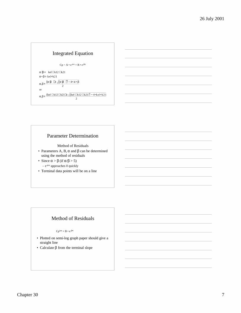
Terminal Slope

0.01

0.1

1

10

100

0 2 4 6 8 10 12 14 16 18 20 22 24

Con

cent

ratio

n (m

g/L)

Time (hr)

Cp = 24 • e-1.5•t + 6 • e-0.25•t

slope > β

Terminal Half-life

• t1/2 = ln(2)/β• Biological or terminal half-life

• [= equivalent to ln(2)/kel with onecompartment model]

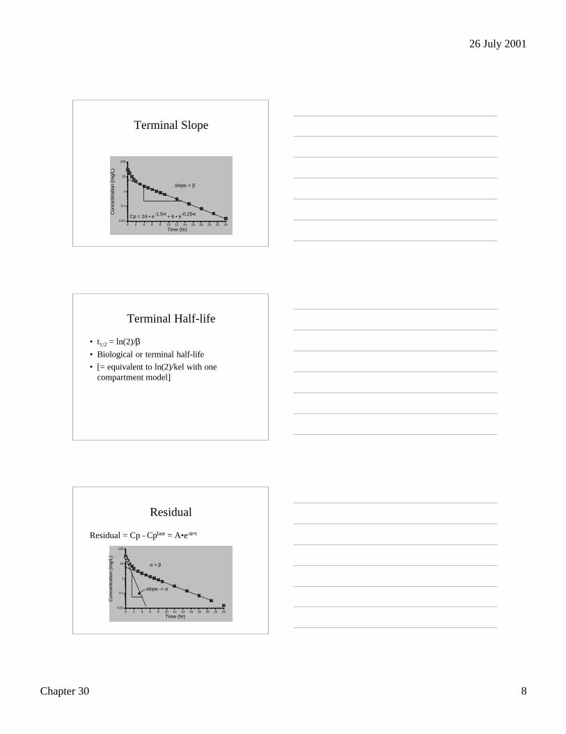
Residual

Residual = Cp - Cplate = A•e-α•t

0.01

0.1

1

10

100

0 2 4 6 8 10 12 14 16 18 20 22 24

Con

cent

ratio

n (m

g/L)

Time (hr)

slope -> α

α > β

26 July 2001

Chapter 30 9

Now Calculate k21, kel, k12

k21 = A• β+ B• αA + B

kel =α •βk21

k12 = α + β − k21 − kel

Effect of k12 and k21 Ratio

0

1

2

3

4

5

6

7

8

9

10

0 1 2 3 4

Con

cent

ratio

n (m

g/L)

Time (hour)

k12/k21 = 1/4

k12/k21 = 1/2

k12/k21 = 1/1

k12/k21 = 2/1

k12/k21 = 4/1

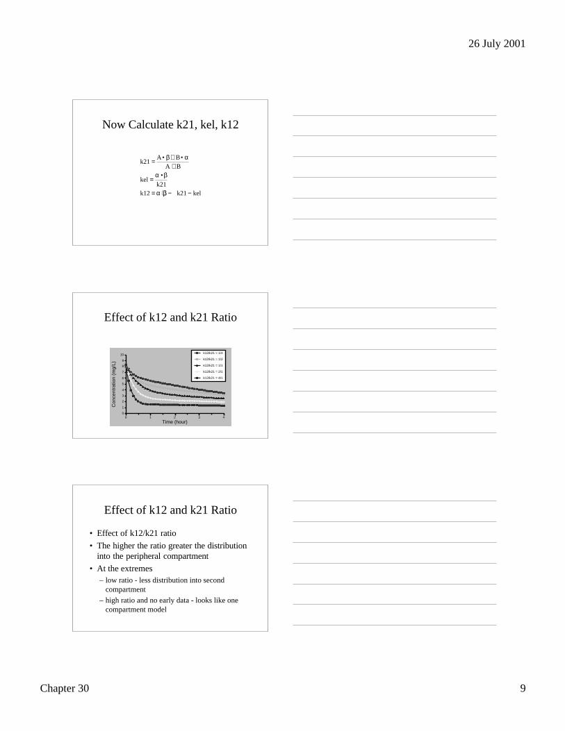
Effect of k12 and k21 Ratio

• Effect of k12/k21 ratio

• The higher the ratio greater the distributioninto the peripheral compartment

• At the extremes– low ratio - less distribution into second

compartment

– high ratio and no early data - looks like onecompartment model

26 July 2001

Chapter 30 10

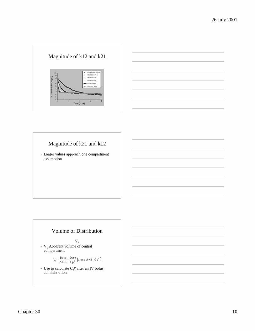
Magnitude of k12 and k21

0

1

2

3

4

5

6

7

8

9

10

0 1 2 3 4

Con

cent

ratio

n (m

g/L)

Time (hour)

k12/k21 = 0.5/0.25

k12/k21 = 1/0.5

k12/k21 = 2/1

k12/k21 = 4/2

k12/k21 = 8/4

k12/21 = 16/8

Magnitude of k21 and k12

• Larger values approach one compartmentassumption

Volume of Distribution

V1

• V1 Apparent volume of centralcompartment

• Use to calculate Cp0 after an IV bolusadministration

V1 =Dose

A + B=

Dose

Cp0 since A+B=Cp0( )

26 July 2001

Chapter 30 11

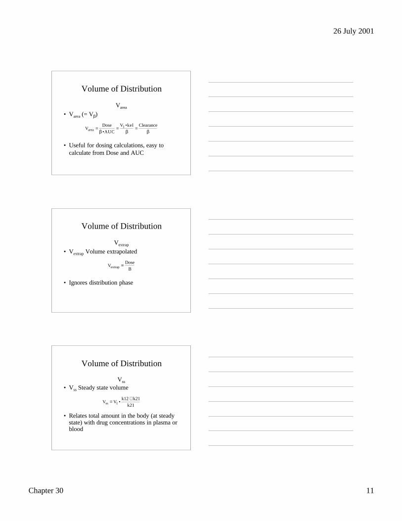
Volume of Distribution

Varea

• Varea (= Vβ)

• Useful for dosing calculations, easy tocalculate from Dose and AUC

Varea =Dose

β •AUC=

V1 •kel

β=

Clearance

β

Volume of Distribution

Vextrap

• Vextrap Volume extrapolated

• Ignores distribution phase

Vextrap =Dose

B

Volume of Distribution

Vss

• Vss Steady state volume

• Relates total amount in the body (at steadystate) with drug concentrations in plasma orblood

Vss = V1 •k12 + k21

k21

26 July 2001

Chapter 30 12

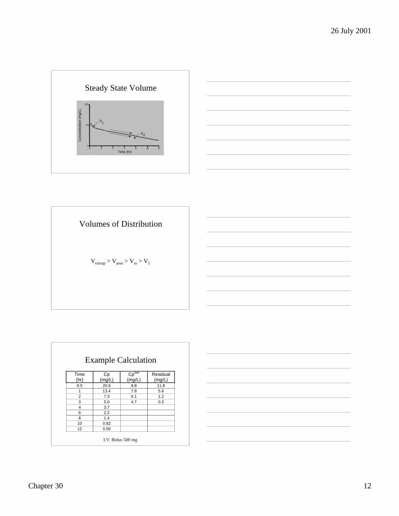
Steady State Volume

1

10

100

0 2 4 6 8 10 12

Con

cent

ratio

n (m

g/L)

Time (hr)

X1

X2

Volumes of Distribution

Vextrap > Varea > Vss > V1

I.V. Bolus 500 mg

Example Calculation

Time(hr)

Cp(mg/L)

Cplate

(mg/L)Residual(mg/L)

0.5 20.6 8.8 11.81 13.4 7.8 5.62 7.3 6.1 1.23 5.0 4.7 0.34 3.76 2.28 1.410 0.8212 0.50

26 July 2001

Chapter 30 13

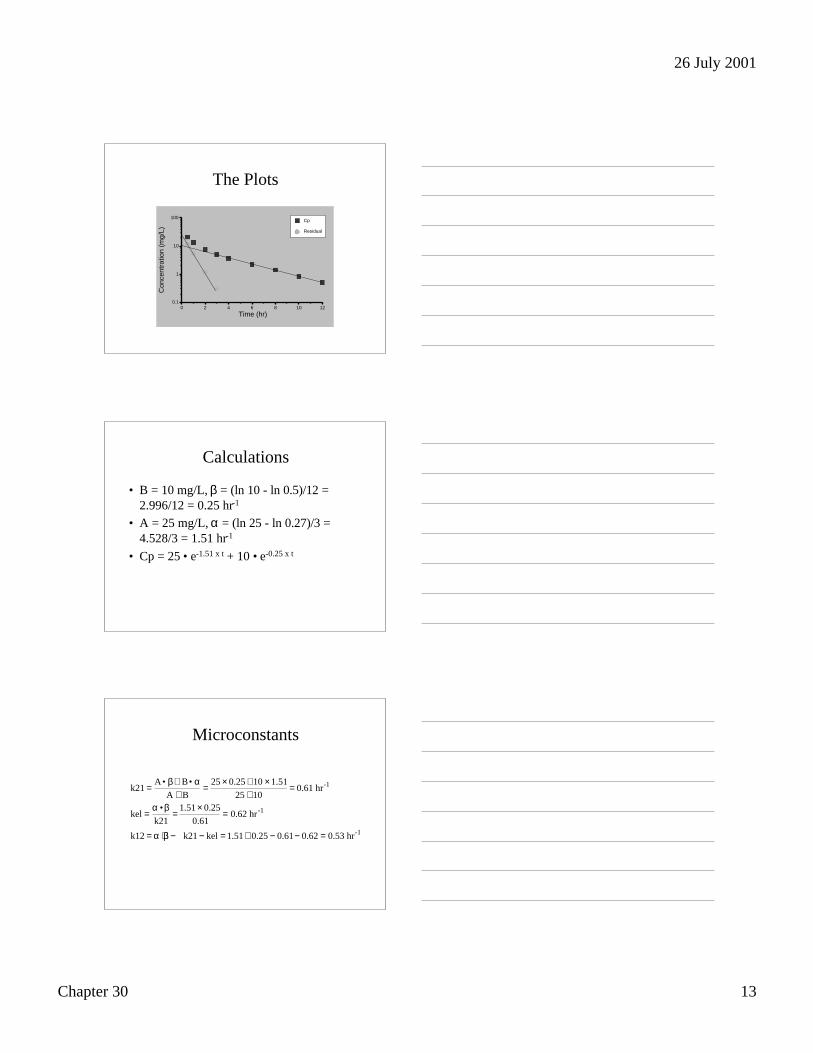
The Plots

0.1

1

10

100

0 2 4 6 8 10 12

Con

cent

ratio

n (m

g/L)

Time (hr)

Cp

Residual

Calculations

• B = 10 mg/L, β = (ln 10 - ln 0.5)/12 =2.996/12 = 0.25 hr-1

• A = 25 mg/L, α = (ln 25 - ln 0.27)/3 =4.528/3 = 1.51 hr-1

• Cp = 25 • e-1.51 x t + 10 • e-0.25 x t

Microconstants

k21 =A• β+ B• α

A + B=

25 × 0.25 + 10 × 1.51

25 + 10= 0.61 hr-1

kel =α •βk21

=1.51 × 0.25

0.61= 0.62 hr -1

k12 = α + β − k21 − kel = 1.51 + 0.25 − 0.61− 0.62 = 0.53 hr-1

26 July 2001

Chapter 30 14

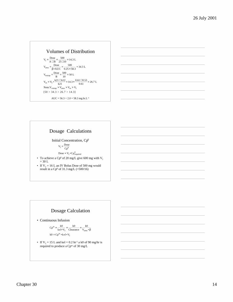
Volumes of Distribution

AUC = 56.3 + 2.0 = 58.3 mg.hr.L -1

V1 = DoseA + B

= 50025 +10

= 14.3 L

Varea = Dose

β •AUC= 500

0.25 × 58.3= 34.3 L

Vextrap = DoseB

= 50010

= 50 L

Vss = V1 •k21 + k12

k21= 14.3 × 0.61 + 0.53

0.61= 26.7 L

Note:Vextrap > Varea > Vss > V1

[50 > 34.3 > 26.7 > 14.3]

Dosage Calculations

Initial Concentration, Cp0

• To achieve a Cp0 of 20 mg/L give 600 mg with V1= 30 L

• If V1 = 16 L an IV Bolus Dose of 500 mg wouldresult in a Cp0 of 31.3 mg/L (=500/16)

V1 = Dose

Cp0

Dose = V1 •Cprequired0

Dosage Calculation

• Continuous Infusion

• If V1 = 15 L and kel = 0.2 hr-1 a k0 of 90 mg/hr isrequired to produce a Cpss of 30 mg/L

Cpss = k0kel•V1

= k0Clearance

= k0Varea • β

k0 = Cpss •ke l •V1

26 July 2001

Chapter 30 15

Plasma Concentration

Time to Steady State

• Cp can be calculated after an IV bolus dosefrom A, B, α and β

• Cp after an IV infusion somewhat moreinvolved

• Time to steady state controlled by β value

• Can be slow with long biological half-life

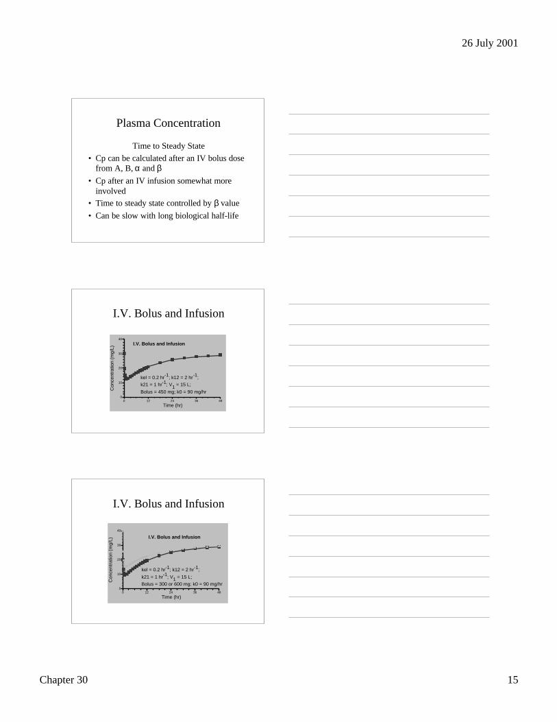
I.V. Bolus and Infusion

0

10

20

30

40

0 12 24 36 48

Con

cent

ratio

n (m

g/L)

Time (hr)

I.V. Bolus and Infusion

kel = 0.2 hr-1; k12 = 2 hr-1;

k21 = 1 hr-1; V1 = 15 L;

Bolus = 450 mg; k0 = 90 mg/hr

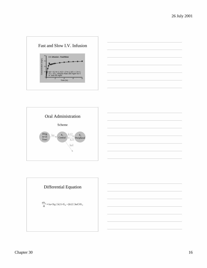
I.V. Bolus and Infusion

0

10

20

30

40

0 12 24 36 48

Con

cent

ratio

n (m

g/L)

Time (hr)

I.V. Bolus and Infusion

kel = 0.2 hr-1; k12 = 2 hr-1;

k21 = 1 hr-1; V1 = 15 L;

Bolus = 300 or 600 mg; k0 = 90 mg/hr

26 July 2001

Chapter 30 16

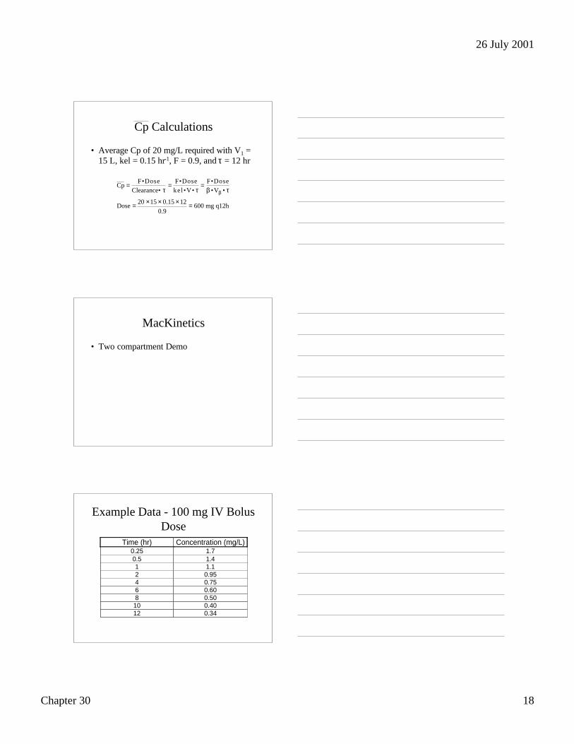
Fast and Slow I.V. Infusion

0

10

20

30

40

0 12 24 36 48

Con

cent

ratio

n (m

g/L)

Time (hr)

I.V. Infusion - Fast/Slow

kel = 0.2 hr-1; k12 = 2 hr-1; k21 = 1 hr-1;V1 = 15 L; Infusion Rate 300 mg/hr for 4hr then 90 mg/hr

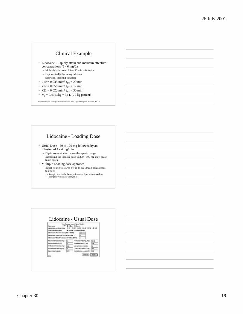
Oral Administration

Scheme

ka

kel

k12

k21

Drugin GITract

X1

CentralX2

Peripheral

Differential Equation

dX1

dt= ka•Xg + k21•X2 − k12 + kel( ) •X 1

26 July 2001

Chapter 30 17

Semi-log Plot

1

10

100

0 12 24 36 48

Con

cent

ratio

n (m

g/L)

Time (hr)

Oral - Two Compartmentwith Distribution Phase

A = 20 mg/L; B = 15 mg/L;

C = -35 mg/L; α = 1 hr-1;

β = 0.1 hr-1; ka = 2 hr-1

Semi-log Plot

0.001

0.01

0.1

1

10

0 12 24 36 48

Con

cent

ratio

n (m

g/L)

Time (hr)

Oral - Two Compartmentwithout Distribution Phase

A = 20 mg/L; B = 15 mg/L; C = -35 mg/L;

α = 1.5 hr-1; β = 0.16 hr-1; ka = 1 hr-1

Oral Dose

Two Compartment Model• Bioavailability calculations the same as for a one

compartment model– Use AUC comparison or– Use U∞ comparison

• These method work for any linear system (first orderdisposition)

• Method of residuals could be used to calculate α, β,and ka (if sufficiently different)

26 July 2001

Chapter 30 18

Cp Calculations

• Average Cp of 20 mg/L required with V1 =15 L, kel = 0.15 hr-1, F = 0.9, and τ = 12 hr

Cp = F•DoseClearance• τ

= F•Dosekel•V• τ

= F•Doseβ •Vβ • τ

Dose = 20 ×15 × 0.15 ×12

0.9= 600 mg q12h

MacKinetics

• Two compartment Demo

Example Data - 100 mg IV BolusDose

Time (hr) Concentration (mg/L)0.25 1.70.5 1.41 1.12 0.954 0.756 0.608 0.50

10 0.4012 0.34

26 July 2001

Chapter 30 19

Clinical Example

• Lidocaine - Rapidly attain and maintain effectiveconcentrations (2 - 6 mg/L)– Multiple bolus over 15 or 30 min + infusion– Exponentially declining infusion– Stepwise, tapering infusion

• k10 = 0.035 min-1 t1/2 = 20 min• k12 = 0.058 min-1 t1/2 = 12 min• k21 = 0.023 min-1 t1/2 = 30 min• V1 = 0.49 L/kg = 34 L (70 kg patient)

Evans, Schentag, and Jusko Applied Pharmacokinetics, 3rd ed., Applied Therapeutics, Vancouver, WA 1992

Lidocaine - Loading Dose

• Usual Dose - 50 to 100 mg followed by aninfusion of 1 - 4 mg/min– Dip in concentration below therapeutic range– Increasing the loading dose to 200 - 300 mg may cause

toxic doses

• Multiple Loading dose approach– Initial 75 mg followed by up to six 50 mg bolus doses

to effect• Ectopic ventricular beats to less than 5 per minute and no

complex ventricular arrhymias

Lidocaine - Usual Dosemin x

26 July 2001

Chapter 30 20

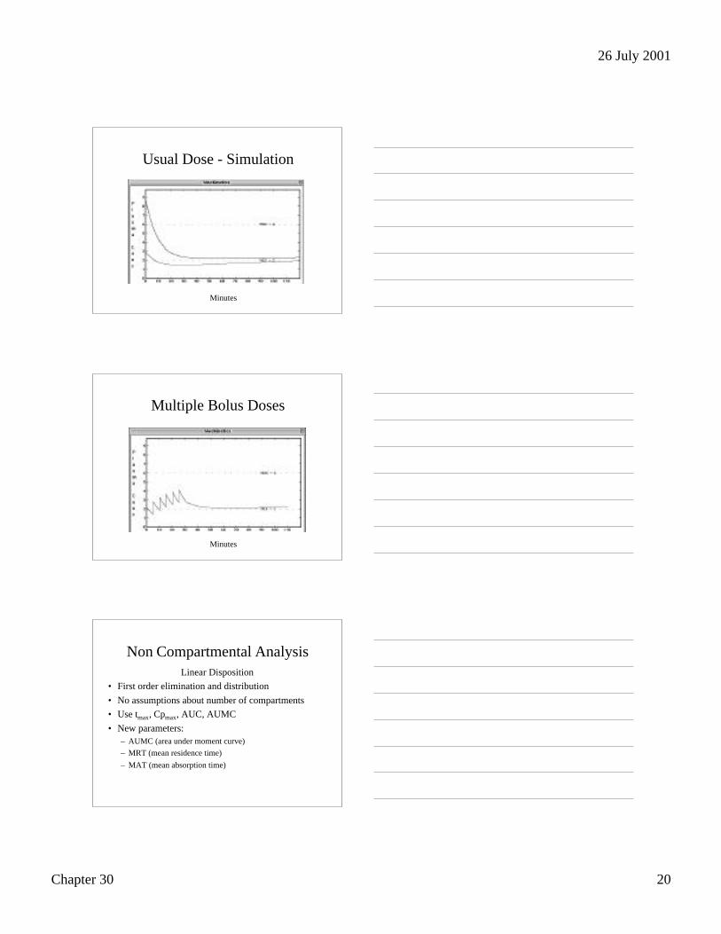
Usual Dose - Simulation

Minutes

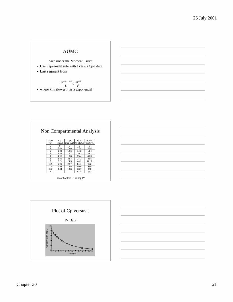
Multiple Bolus Doses

Minutes

Non Compartmental AnalysisLinear Disposition

• First order elimination and distribution

• No assumptions about number of compartments

• Use tmax, Cpmax, AUC, AUMC

• New parameters:– AUMC (area under moment curve)

– MRT (mean residence time)

– MAT (mean absorption time)

26 July 2001

Chapter 30 21

AUMC

Area under the Moment Curve

• Use trapezoidal rule with t versus Cp•t data

• Last segment from

• where k is slowest (last) exponential

Cplast • t last

k+

Cplast

k2

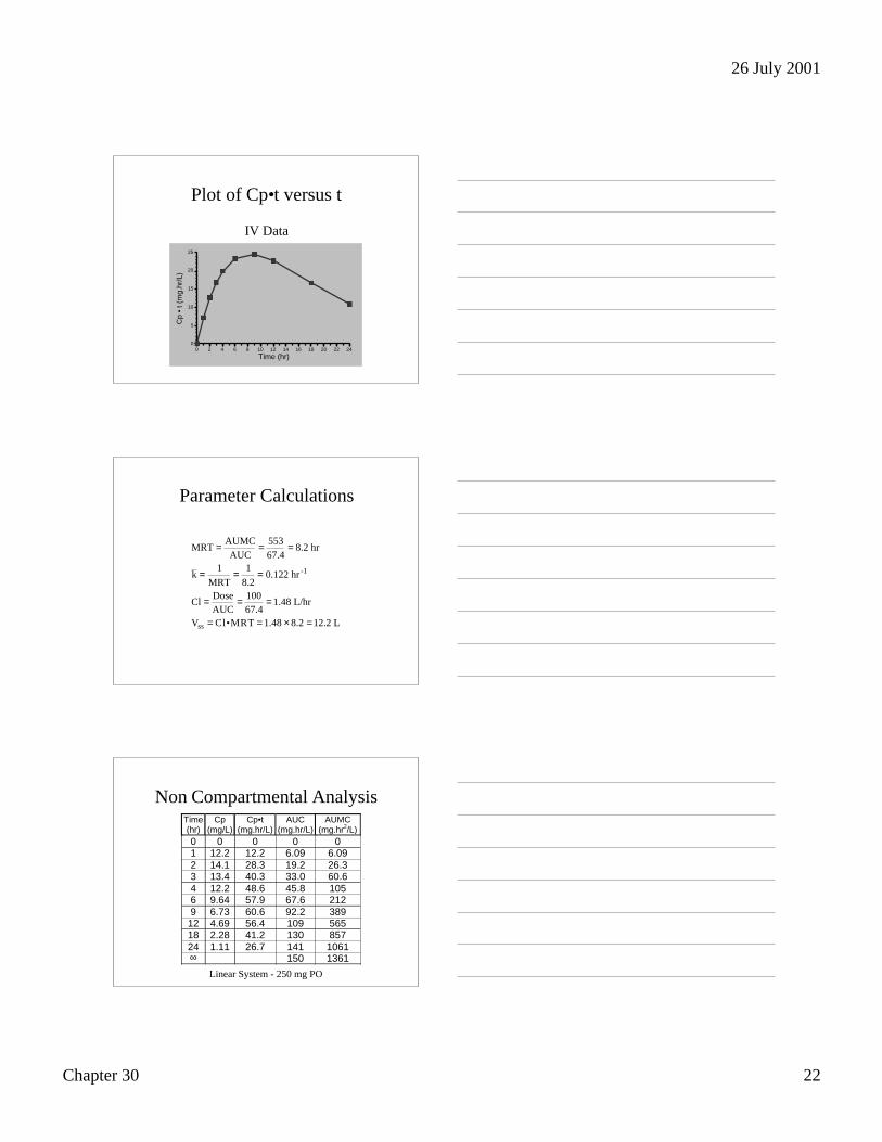
Non Compartmental Analysis

Linear System - 100 mg IV

Time(hr)

Cp(mg/L)

Cp•t(mg.hr/L)

AUC(mg.hr/L)

AUMC(mg.hr2/L)

0 0 0 0 01 7.09 7.09 7.54 3.542 6.29 12.6 14.2 13.43 5.58 16.7 20.2 28.14 4.95 19.8 25.4 46.36 3.89 23.4 34.3 89.59 2.71 24.5 44.2 161.212 1.89 22.7 51.1 23218 0.92 16.6 59.6 35024 0.44 10.8 63.7 432∞ 67.4 553

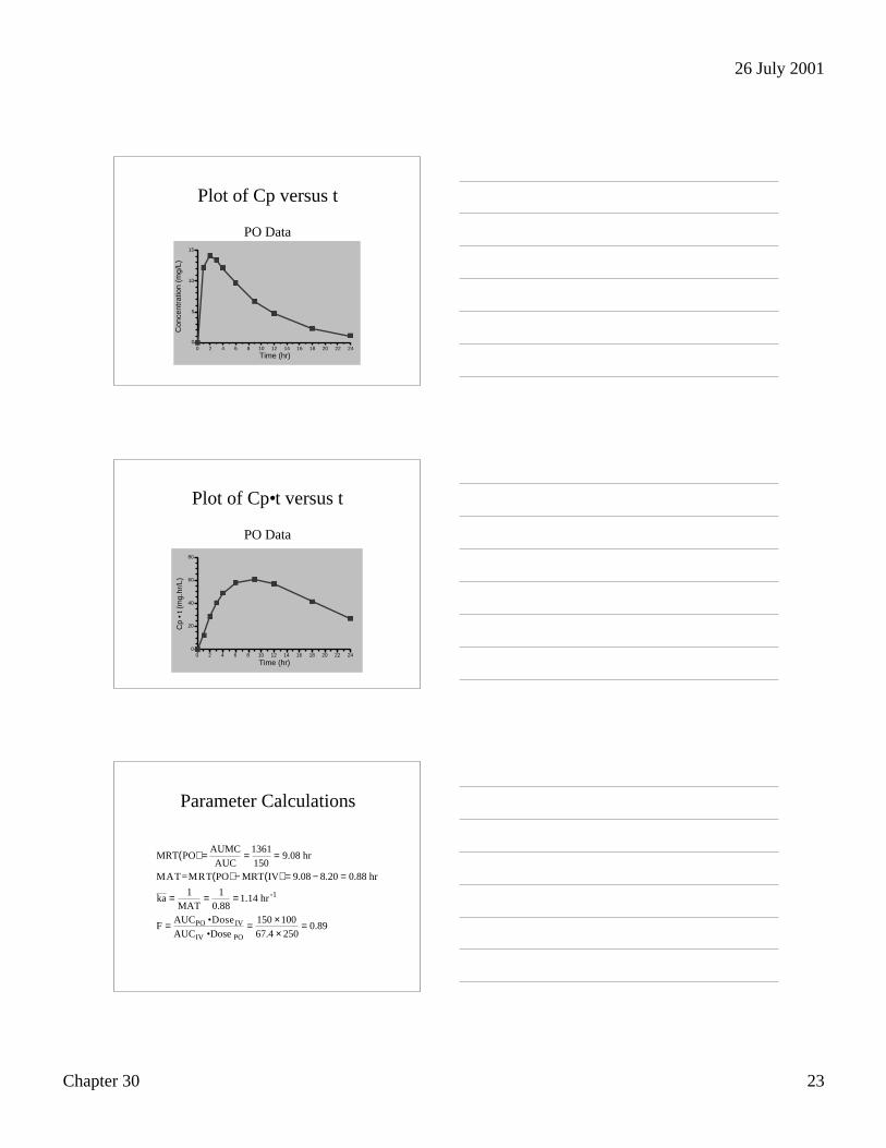
Plot of Cp versus t

IV Data

0

2

4

6

8

10

0 2 4 6 8 10 12 14 16 18 20 22 24

Con

cent

ratio

n (m

g/L)

Time (hr)

26 July 2001

Chapter 30 22

Plot of Cp•t versus t

IV Data

0

5

10

15

20

25

0 2 4 6 8 10 12 14 16 18 20 22 24

Cp

• t (

mg.

hr/L

)

Time (hr)

Parameter Calculations

MRT = AUMCAUC

= 55367.4

= 8.2 hr

k = 1

MRT= 1

8.2= 0.122 hr -1

Cl = DoseAUC

= 10067.4

= 1.48 L/hr

Vss = Cl•MRT = 1.48 × 8.2 =12.2 L

Non Compartmental Analysis

Linear System - 250 mg PO

Time(hr)

Cp(mg/L)

Cp•t(mg.hr/L)

AUC(mg.hr/L)

AUMC(mg.hr2/L)

0 0 0 0 01 12.2 12.2 6.09 6.092 14.1 28.3 19.2 26.33 13.4 40.3 33.0 60.64 12.2 48.6 45.8 1056 9.64 57.9 67.6 2129 6.73 60.6 92.2 389

12 4.69 56.4 109 56518 2.28 41.2 130 85724 1.11 26.7 141 1061∞ 150 1361

26 July 2001

Chapter 30 23

Plot of Cp versus t

PO Data

0

5

10

15

0 2 4 6 8 10 12 14 16 18 20 22 24

Con

cent

ratio

n (m

g/L)

Time (hr)

Plot of Cp•t versus t

PO Data

0

20

40

60

80

0 2 4 6 8 10 12 14 16 18 20 22 24

Cp

• t (

mg.

hr/L

)

Time (hr)

Parameter Calculations

MRT PO( ) = AUMCAUC

= 1361150

= 9.08 hr

MAT=MRT PO( ) − MRT IV( ) = 9.08 − 8.20 = 0.88 hr

ka = 1MAT

= 10.88

= 1.14 hr -1

F = AUCPO •Dose IV

AUCIV •Dose PO= 150 × 100

67.4 × 250= 0.89

26 July 2001

Chapter 30 24

Objectives

• To draw schemes and write differential equationsfor multicompartment models

• To recognize and use integrated equations tocalculate dosage regimens

• To determine parameter values using the methodof residuals

• To calculate various V values• To use the non-compartmental method of

parameter estimation