Multidimensional Scaling

Patrick J.F. Groenen∗ Michel van de Velden †

April 6, 2004

Econometric Institute Report EI 2004-15

Abstract

Multidimensional scaling is a statistical technique to visualize dissimi-larity data. In multidimensional scaling, objects are represented as pointsin a usually two dimensional space, such that the distances between thepoints match the observed dissimilarities as closely as possible. Here, wediscuss what kind of data can be used for multidimensional scaling, whatthe essence of the technique is, how to choose the dimensionality, trans-formations of the dissimilarities, and some pitfalls to watch out for whenusing multidimensional scaling.

1 Introduction

Multidimensional scaling is a statistical technique originating in psychometrics.The data used for multidimensional scaling (MDS) are dissimilarities betweenpairs of objects. The main objective of MDS is to represent these dissimilaritiesas distances between points in a low dimensional space such that the distancescorrespond as closely as possible to the dissimilarities.

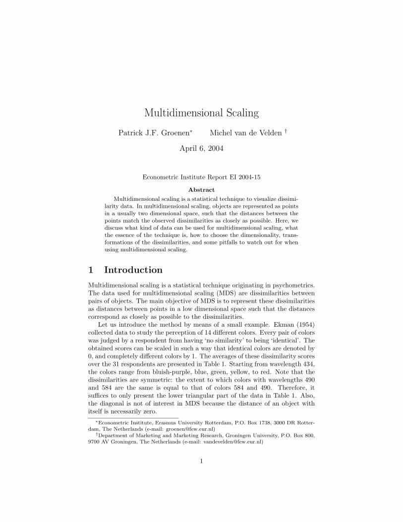
Let us introduce the method by means of a small example. Ekman (1954)collected data to study the perception of 14 different colors. Every pair of colorswas judged by a respondent from having ‘no similarity’ to being ‘identical’. Theobtained scores can be scaled in such a way that identical colors are denoted by0, and completely different colors by 1. The averages of these dissimilarity scoresover the 31 respondents are presented in Table 1. Starting from wavelength 434,the colors range from bluish-purple, blue, green, yellow, to red. Note that thedissimilarities are symmetric: the extent to which colors with wavelengths 490and 584 are the same is equal to that of colors 584 and 490. Therefore, itsuffices to only present the lower triangular part of the data in Table 1. Also,the diagonal is not of interest in MDS because the distance of an object withitself is necessarily zero.

∗Econometric Institute, Erasmus University Rotterdam, P.O. Box 1738, 3000 DR Rotter-dam, The Netherlands (e-mail: groenen@few.eur.nl)

†Department of Marketing and Marketing Research, Groningen University, P.O. Box 800,9700 AV Groningen, The Netherlands (e-mail: vandevelden@few.eur.nl)

1

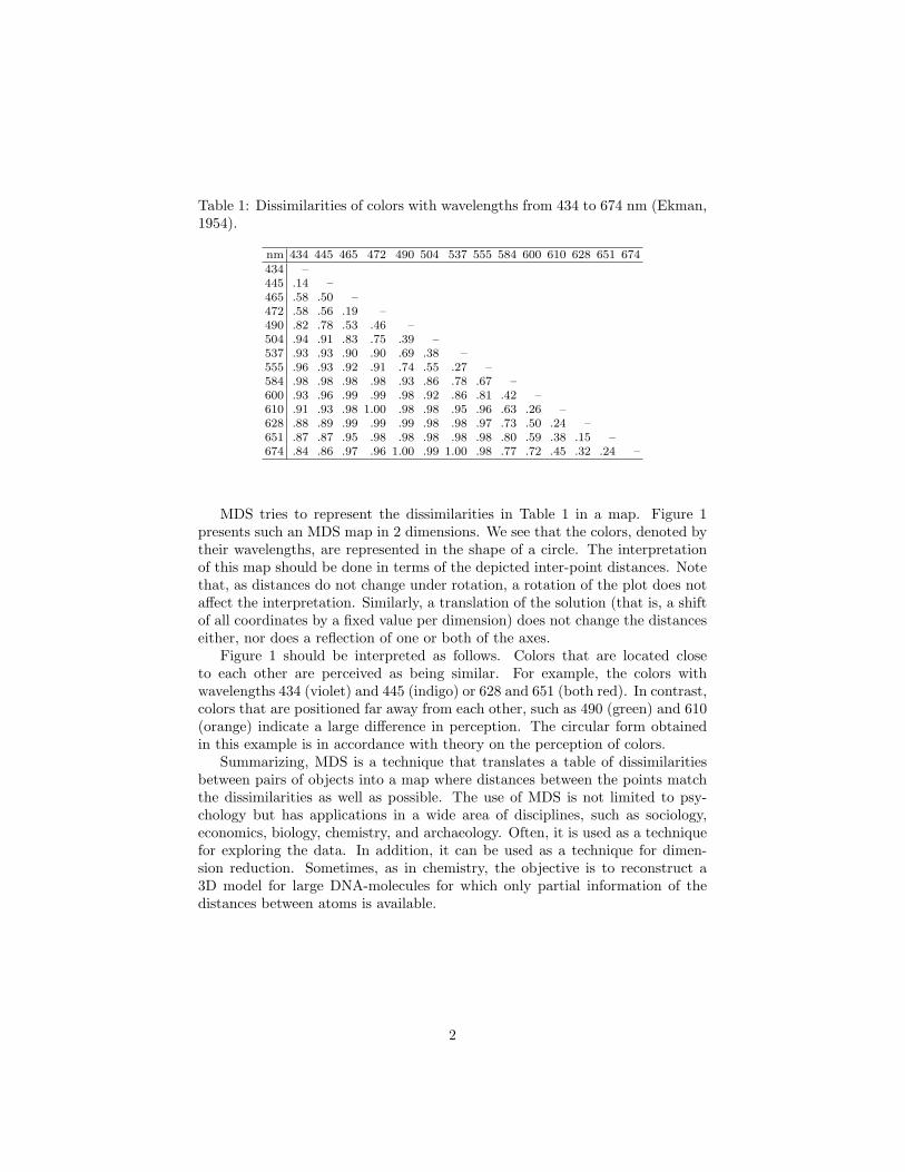
Table 1: Dissimilarities of colors with wavelengths from 434 to 674 nm (Ekman,1954).

nm 434 445 465 472 490 504 537 555 584 600 610 628 651 674434 –445 .14 –465 .58 .50 –472 .58 .56 .19 –490 .82 .78 .53 .46 –504 .94 .91 .83 .75 .39 –537 .93 .93 .90 .90 .69 .38 –555 .96 .93 .92 .91 .74 .55 .27 –584 .98 .98 .98 .98 .93 .86 .78 .67 –600 .93 .96 .99 .99 .98 .92 .86 .81 .42 –610 .91 .93 .98 1.00 .98 .98 .95 .96 .63 .26 –628 .88 .89 .99 .99 .99 .98 .98 .97 .73 .50 .24 –651 .87 .87 .95 .98 .98 .98 .98 .98 .80 .59 .38 .15 –674 .84 .86 .97 .96 1.00 .99 1.00 .98 .77 .72 .45 .32 .24 –

MDS tries to represent the dissimilarities in Table 1 in a map. Figure 1presents such an MDS map in 2 dimensions. We see that the colors, denoted bytheir wavelengths, are represented in the shape of a circle. The interpretationof this map should be done in terms of the depicted inter-point distances. Notethat, as distances do not change under rotation, a rotation of the plot does notaffect the interpretation. Similarly, a translation of the solution (that is, a shiftof all coordinates by a fixed value per dimension) does not change the distanceseither, nor does a reflection of one or both of the axes.

Figure 1 should be interpreted as follows. Colors that are located closeto each other are perceived as being similar. For example, the colors withwavelengths 434 (violet) and 445 (indigo) or 628 and 651 (both red). In contrast,colors that are positioned far away from each other, such as 490 (green) and 610(orange) indicate a large difference in perception. The circular form obtainedin this example is in accordance with theory on the perception of colors.

Summarizing, MDS is a technique that translates a table of dissimilaritiesbetween pairs of objects into a map where distances between the points matchthe dissimilarities as well as possible. The use of MDS is not limited to psy-chology but has applications in a wide area of disciplines, such as sociology,economics, biology, chemistry, and archaeology. Often, it is used as a techniquefor exploring the data. In addition, it can be used as a technique for dimen-sion reduction. Sometimes, as in chemistry, the objective is to reconstruct a3D model for large DNA-molecules for which only partial information of thedistances between atoms is available.

2

434445

465472490

504

537

555

584600 610

628651

674

Figure 1: MDS solution in 2 dimensions of the color data in Table 1.

2 Data for MDS

In the previous section, we introduced MDS as a method to describe relation-ships between objects on the basis of observed dissimilarities. However, insteadof dissimilarities we often observe similarities between objects. Correlations, forexample, can be interpreted as similarities. By converting the similarities intodissimilarities MDS can easily be applied to similarity data. There are severalways of transforming similarities into dissimilarities. For example, we may takeone divided by the similarity or we can apply any monotone decreasing functionthat yields nonnegative values (dissimilarities cannot be negative). However, inSection 4, we shall see that by applying transformations in MDS, there is noneed to transform similarities into dissimilarities. To indicate both similarityand dissimilarity data, we use the generic term proximities.

Data in MDS can be obtained in a variety of ways. We distinguish betweenthe direct collection of proximities versus derived proximities. The color dataof the previous section is an example of direct proximities. That is, the dataarrives in the format of proximities. Often, this is not the case and our datadoes not consist of proximities between variables. However, by considering anappropriate measure, proximities can be derived from the original data. Forexample, consider the case where objects are rated on several variables. Ifthe interest lies in representing the variables, we can calculate the correlationmatrix as measure of similarity between the variables. MDS can be appliedto describe the relationship between the variables on the basis of the derivedproximities. Alternatively, if interest lies in the objects, Euclidean distancescan be computed between the objects using the variables as dimensions. In thiscase, we use high dimensional Euclidean distances as dissimilarities and we canuse MDS to reconstruct these distances in a low dimensional space.

3

Co-occurrence data are another source for obtaining dissimilarities. For suchdata, a respondent groups the objects into partitions and an n × n incidencematrix is derived where a one indicates that a pair of objects is in the samegroup and a zero indicates that they are in different groups. By consideringthe frequencies of objects being in the same or different groups and by applyingspecial measures (such as the so-called Jaccard similarity measure), we obtainproximities. For a detailed discussion of various (dis)similarity measures, werefer to Gower and Legendre (1986).

3 Formalizing Multidimensional Scaling

To formalize MDS, we need some notation. Let n be the number of differentobjects and let the dissimilarity for objects i and j be given by δij . The coor-dinates are gathered in an n× p matrix X, where p is the dimensionality of thesolution to be specified in advance by the user. Thus, row i from X gives thecoordinates for object i. Let dij(X) be the Euclidean distance between rows iand j of X defined as

dij(X) =

(p∑

s=1

(xis − xjs)2)1/2

, (1)

that is, the length of the shortest line connecting points i and j. The objective ofMDS is to find a matrix X such that dij(X) matches δij as closely as possible.This objective can be formulated in a variety of ways but here we use thedefinition of raw-Stress σ2(X), that is,

σ2(X) =n∑

i=2

i−1∑

j=1

wij(δij − dij(X))2 (2)

by Kruskal (Kruskal, 1964a, 1964b) who was the first one to propose a formalmeasure for doing MDS. This measure is also referred to as the least-squaresMDS model. Note that due to the symmetry of the dissimilarities and thedistances, the summation only involves the pairs ij where i > j. Here, wij

is a user defined weight that must be nonnegative. For example, many MDSprograms implicitly choose wij = 0 for dissimilarities that are missing.

The minimization of σ2(X) is a rather complex problem that cannot besolved in closed-form. Therefore, MDS programs use iterative numerical algo-rithms to find a matrix X for which σ2(X) is a minimum. One of the best algo-rithms available is the SMACOF algorithm (De Leeuw, 1977, 1988; De Leeuw& Heiser, 1980; Borg & Groenen, 1997) based on iterative majorization. TheSMACOF algorithm has been implemented in the SPSS procedure Proxscal(Meulman, Heiser, & SPSS, 1999). In Section 7, we give a brief illustration ofthe SMACOF algorithm.

Because Euclidean distances do not change under rotation, translation, andreflection, these operations may be freely applied to MDS solution without af-fecting the raw-Stress. Many MDS programs use this indeterminacy to center

4

the coordinates so that they sum to zero dimension wise. The freedom of rota-tion is often exploited to put the solution in so-called principal axis orientation.That is, the axis are rotated in such a way that the variance of X is maximalalong the first dimension, the second dimension is uncorrelated to the first andhas again maximal variance, and so on.

Here, we have discussed the Stress measure for MDS. However, there areseveral other measures for doing MDS. In Section 8, we briefly discuss otherpopular definitions of Stress.

4 Transformations of the Data

So far, we have assumed that the dissimilarities are known. However, this isoften not the case. Consider for example the situation in which the objects havebeen ranked. That is, the dissimilarities between the objects are not known, buttheir order is known. In such a case, we would like to assign numerical valuesto the proximities in such a way that these values exhibit the same rank orderas the data. These numerical values are usually called disparities, d-hats, orpseudo distances, and they are denoted by d̂. The task of MDS now becomesto simultaneously obtain disparities and coordinates in such a way that thecoordinates represent the disparities (and thus the original rank order of thedata) as well as possible. This objective can be captured in minimizing a slightadaptation of raw Stress, that is,

σ2(d̂,X) =n∑

i=2

i−1∑

j=1

wij(d̂ij − dij(X))2, (3)

over both the d̂ and X, where d̂ is the vector containing d̂ij for all pairs.The process of finding the disparities is called optimal scaling and was firstintroduced by Kruskal (Kruskal, 1964a, 1964b). Optimal scaling aims to find atransformation of the data that fits as well as possible the distances in the MDSsolution. To avoid the trivial optimal scaling solution X = 0 and d̂ij = 0 for allij, we impose a length constraint on the disparities in such a way that the sumof squared d-hat’s equals a fixed constant. For example,

∑ni=2

∑i−1j=1 wij d̂

2ij =

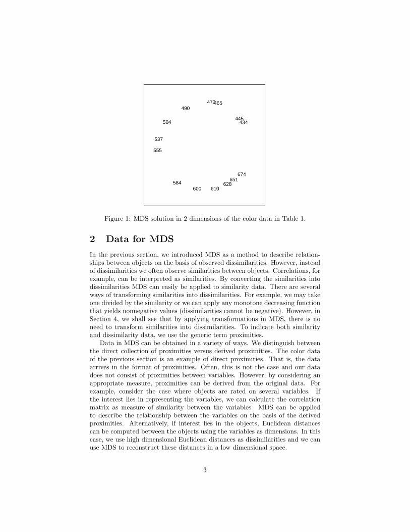
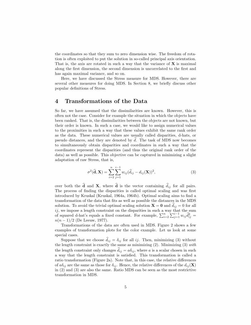
n(n− 1)/2 (De Leeuw, 1977).Transformations of the data are often used in MDS. Figure 2 shows a few

examples of transformation plots for the color example. Let us look at somespecial cases.

Suppose that we choose d̂ij = δij for all ij. Then, minimizing (3) withoutthe length constraint is exactly the same as minimizing (2). Minimizing (3) withthe length constraint only changes d̂ij = aδij , where a is a scalar chosen in sucha way that the length constraint is satisfied. This transformation is called aratio transformation (Figure 2a). Note that, in this case, the relative differencesof aδij are the same as those for δij . Hence, the relative differences of the dij(X)in (2) and (3) are also the same. Ratio MDS can be seen as the most restrictivetransformation in MDS.

5

dij

.0 .2 .4 .6 .8 1.0.0

.2

.4

.6

.8

1.0

1.2

δij

ˆ

dij

.0 .2 .4 .6 .8 1.0.0

.2

.4

.6

.8

1.0

1.2

δij

ˆ dij

.0 .2 .4 .6 .8 1.0.0

.2

.4

.6

.8

1.0

1.2

δij

ˆ

dij

.0 .2 .4 .6 .8 1.0.0

δij

ˆ

.2

.4

.6

.8

1.0

1.2

1.4

a. Ratio b. Interval

c. Ordinal d. Spline

Figure 2: Four transformations often used in MDS.

An obvious extension to the ratio transformation is obtained by allowingthe d̂ij to be a linear transformation of the δij . That is, d̂ij = a + bδij , forsome unknown values of a and b. Figure 2b depicts an interval transformation.This transformation may be chosen if there is reason to believe that δij = 0does not have any particular interpretation. An interval transformation thatis almost horizontal reveals little about the data as different dissimilarities aretransformed to similar disparities. In such a case, the constant term will domi-nate the d̂ij ’s. On the other hand, a good interval transformation is obtained ifthe line is not horizontal and the constant term is reasonably small with respectto the rest.

For ordinal MDS, the d̂ij are only required to have the same rank orderas δij . That is, if for two pairs of objects ij and kl we have δij ≤ δkl thenthe corresponding disparities must satisfy d̂ij ≤ d̂kl. An example of an ordinaltransformation in MDS is given in Figure 2c. Typically, an ordinal transforma-tion shows a step function. Similar to the case for interval transformations, itis not a good sign if the transformation plot shows a horizontal line. Moreover,if the transformation plot only exhibits a few steps, ordinal MDS does not usefiner information available in the data. Ordinal MDS is particularly suited if theoriginal data are rank orders. To compute an ordinal transformation a methodcalled monotone regression can be used.

A monotone spline transformation offers more freedom than an intervaltransformation, but never more than an ordinal transformation. The advan-tage of a spline transformation over an ordinal transformation is that it will

6

yield a smooth transformation. Figure 2d shows an example of a spline trans-formation. A spline transformation is built on two ideas. First, the range of theδij ’s can be subdivided into connected intervals. Then, for each interval, thedata are transformed using a polynomial of a specified degree. For example, asecond-degree polynomial imposes that d̂ij = aδ2

ij +bδij +c. The special featureof a spline is that at the connections of the intervals, the so-called interior knots,the two polynomials connect smoothly. The spline transformation in Figure 2dwas obtained by choosing one interior knot at .90 and by using second-degreepolynomials. For MDS it is important that the transformation is monotoneincreasing. This requirement is automatically satisfied for monotone splines orI-Splines (see, Ramsay, 1988; Borg & Groenen, 1997). For choosing a transfor-mation in MDS it suffices to know that a spline transformation is smooth andnonlinear. The amount of nonlinearity is governed by the number of interiorknots specified. Unless the number of dissimilarities is very large, a few interiorknots for a second-degree spline usually works well.

There are several reasons to use transformations in MDS. One reason con-cerns the fit of the data in low dimensionality. By choosing a transformationthat is less restrictive than the ratio transformation a better fit may be obtained.Alternatively, there may exist theoretical reasons why a transformation of thedissimilarities is desired. Ordered from most to least restrictive transformation,we start with ratio, then interval, spline, and ordinal.

If the data are dissimilarities, then it is necessary that a transformation ismonotone increasing (as in Figure 2) so that pairs with higher dissimilaritiesare indeed modelled by larger distances. Conversely, if the data are similarities,then the transformation should be monotone decreasing so that more similarpairs are modelled by smaller distances. A ratio transformation is not possiblefor similarities. The reason is that the d̂ij ’s must be nonnegative. This impliesthat the transformation must include an intercept.

In the MDS literature, one often encounters the terms metric and nonmetricMDS. Metric MDS refers to the ratio and interval transformations, whereas allother transformations such as ordinal and spline transformations are covered bythe term nonmetric MDS. We believe, however, that it is better to refer directlyto the type of transformation that is used.

There exist other a-priori transformations of the data that are not optimalin the sense described above. That is transformations that are not obtainedby minimizing (3). The advantage of optimal transformations is that the exactform of the transformation is unknown and determined optimally together withthe MDS configuration.

5 Diagnostics

In order to assess the quality of the MDS solution we can study the differencesbetween the MDS solution and the data. One convenient way to do this is byinspecting the so-called Shepard diagram.

A Shepard diagram shows both the transformation and the error. Let

7

Proximities

Dis

tanc

es a

nd d

ispa

ritie

s

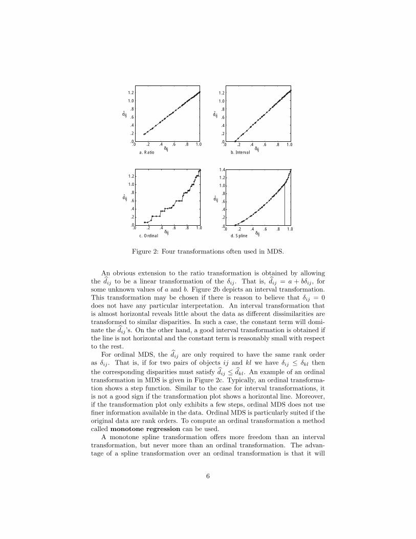
Figure 3: Shepard diagram for ordinal MDS of the color data, where the prox-imities are dissimilarities.

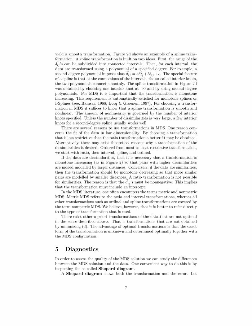
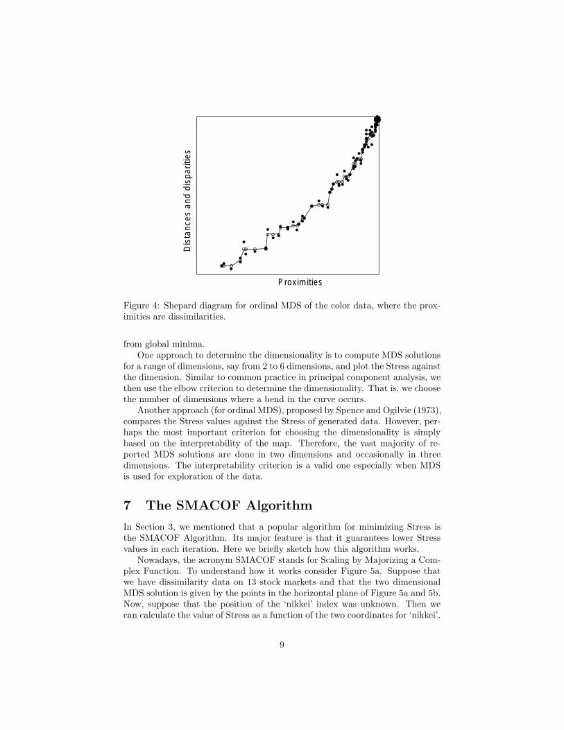
pij denotes the proximity between objects i and j. Then, a Shepard dia-gram plots simultaneously the pairs (pij , dij(X)) and (pij , d̂ij). In Figure 3,solid points denote the pairs (pij , dij(X)) and open circles represent the pairs(pij , d̂ij). By connecting the open circles a line is obtained representing therelationship between the proximities and the disparities which is equivalent tothe transformation plots in Figure 2. The vertical distances between the openand closed circles are equal to d̂ij − dij(X), that is, they give the errors of rep-resentation for each pair of objects. Hence, the Shepard diagram can be usedto inspect both the residuals of the MDS solution and the transformation. Out-liers can be detected as well as possible systematic deviations. Figure 3 givesthe Shepard diagram for the ratio MDS solution of Figure 1 using the colordata. We see that all the errors corresponding to low proximities are positivewhereas the errors for the higher proximities are all negative. This kind of het-eroscedasticity suggests the use of a more liberal transformation. Figure 4 givesthe Shepard diagram for an ordinal transformation. As the solid points arecloser to the line connecting the open circles, we may indeed conclude that theheteroscedasticity has gone and that the fit has become better.

6 Choosing the Dimensionality

Several methods have been proposed to choose the dimensionality of the MDSsolution. However, no definite strategy is present. Unidimensional scaling,that is, p = 1 (with ratio transformation) has to be treated with special carebecause the usual MDS algorithms will end up in local minima that can be far

8

Proximities

Dis

tanc

es a

nd d

ispa

ritie

s

Figure 4: Shepard diagram for ordinal MDS of the color data, where the prox-imities are dissimilarities.

from global minima.One approach to determine the dimensionality is to compute MDS solutions

for a range of dimensions, say from 2 to 6 dimensions, and plot the Stress againstthe dimension. Similar to common practice in principal component analysis, wethen use the elbow criterion to determine the dimensionality. That is, we choosethe number of dimensions where a bend in the curve occurs.

Another approach (for ordinal MDS), proposed by Spence and Ogilvie (1973),compares the Stress values against the Stress of generated data. However, per-haps the most important criterion for choosing the dimensionality is simplybased on the interpretability of the map. Therefore, the vast majority of re-ported MDS solutions are done in two dimensions and occasionally in threedimensions. The interpretability criterion is a valid one especially when MDSis used for exploration of the data.

7 The SMACOF Algorithm

In Section 3, we mentioned that a popular algorithm for minimizing Stress isthe SMACOF Algorithm. Its major feature is that it guarantees lower Stressvalues in each iteration. Here we briefly sketch how this algorithm works.

Nowadays, the acronym SMACOF stands for Scaling by Majorizing a Com-plex Function. To understand how it works consider Figure 5a. Suppose thatwe have dissimilarity data on 13 stock markets and that the two dimensionalMDS solution is given by the points in the horizontal plane of Figure 5a and 5b.Now, suppose that the position of the ‘nikkei’ index was unknown. Then wecan calculate the value of Stress as a function of the two coordinates for ‘nikkei’.

9

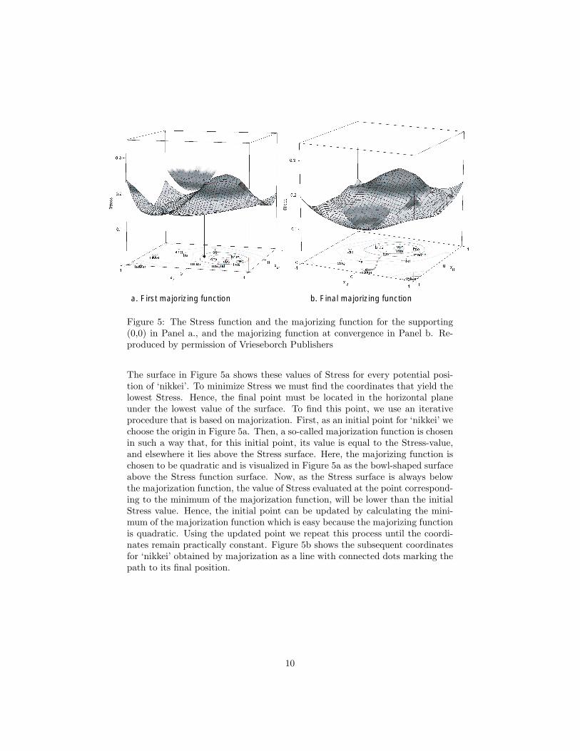
a. First majorizing function b. Final majorizing function

Figure 5: The Stress function and the majorizing function for the supporting(0,0) in Panel a., and the majorizing function at convergence in Panel b. Re-produced by permission of Vrieseborch Publishers

The surface in Figure 5a shows these values of Stress for every potential posi-tion of ‘nikkei’. To minimize Stress we must find the coordinates that yield thelowest Stress. Hence, the final point must be located in the horizontal planeunder the lowest value of the surface. To find this point, we use an iterativeprocedure that is based on majorization. First, as an initial point for ‘nikkei’ wechoose the origin in Figure 5a. Then, a so-called majorization function is chosenin such a way that, for this initial point, its value is equal to the Stress-value,and elsewhere it lies above the Stress surface. Here, the majorizing function ischosen to be quadratic and is visualized in Figure 5a as the bowl-shaped surfaceabove the Stress function surface. Now, as the Stress surface is always belowthe majorization function, the value of Stress evaluated at the point correspond-ing to the minimum of the majorization function, will be lower than the initialStress value. Hence, the initial point can be updated by calculating the mini-mum of the majorization function which is easy because the majorizing functionis quadratic. Using the updated point we repeat this process until the coordi-nates remain practically constant. Figure 5b shows the subsequent coordinatesfor ‘nikkei’ obtained by majorization as a line with connected dots marking thepath to its final position.

10

8 Alternative measures for doing Multidimen-sional Scaling

In addition to the raw Stress measure introduced in Section 3, there exist othermeasures for doing Stress. Here we give a short overview of some of the mostpopular alternatives. First, we discuss normalized raw Stress,

σ2n(d̂,X) =

∑ni=2

∑i−1j=1 wij(d̂ij − dij(X))2

∑ni=2

∑i−1j=1 wij d̂2

ij

, (4)

which is simply raw Stress divided by the sum of squared dissimilarities. Theadvantage of this measure over raw Stress is that its value is independent of thescale and the number of dissimilarities. Thus, multiplying the dissimilarities bya positive factor will not change (4) at a local minimum, whereas the coordinateswill be the same up to the same factor.

The second measure is Kruskal’s Stress-1 formula

σ1(d̂,X) =

(∑ni=2

∑i−1j=1 wij(d̂ij − dij(X))2

∑ni=2

∑i−1j=1 wijd2

ij(X)

)1/2

, (5)

which is equal to the square root of raw Stress divided by the sum of squareddistances. This measure is of importance because many MDS programs andpublications report this value. It can be proved that at a local minimum ofσ2

n(d̂,X), σ1(d̂,X) also has a local minimum with the same configuration up toa multiplicative constant. In addition, the square root of normalized raw Stressis equal to Stress-1 (Borg & Groenen, 1997).

A third measure is Kruskal’s Stress-2, which is similar to Stress-1 exceptthat the denominator is based on the variance of the distances instead of thesum of squares. Stress-2 can be used to avoid the situation where all distancesare almost equal.

A final measure that seems reasonably popular is called S-Stress (imple-mented in the program ALSCAL) and it measures the sum of squared er-ror between squared distances and squared dissimilarities (Takane, Young, &De Leeuw, 1977). The disadvantage of this measure is that it tends to givesolutions in which large dissimilarities are overemphasized and the small dis-similarities are not well represented.

9 Pitfalls

If missing dissimilarities are present, a special problem may occur for certainpatterns of missing dissimilarities. For example, if it is possible to split theobjects in two or more sets such that the between-set weights wij are all zero,we are dealing with independent MDS problems, one for each set. If this situa-tion is not recognized, you may inadvertently interpret the missing between setdistances. With only a few missing values, this situation is unlikely to happen.

11

q q q q q q q q q q q q q q q q q q q q q q q q q q q q q qq

qq

qq

qq

q qq

qq

q

q

qq

q

q

qqq

q

q q

q qq

q

qq

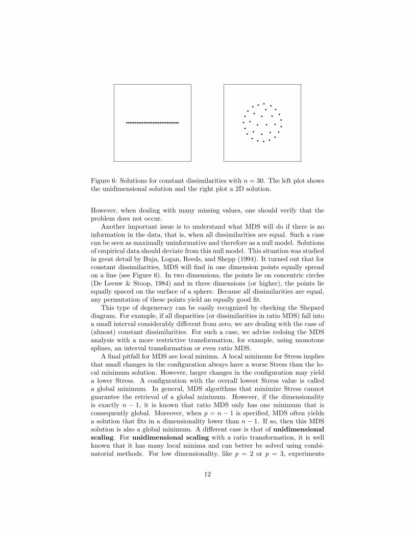
Figure 6: Solutions for constant dissimilarities with n = 30. The left plot showsthe unidimensional solution and the right plot a 2D solution.

However, when dealing with many missing values, one should verify that theproblem does not occur.

Another important issue is to understand what MDS will do if there is noinformation in the data, that is, when all dissimilarities are equal. Such a casecan be seen as maximally uninformative and therefore as a null model. Solutionsof empirical data should deviate from this null model. This situation was studiedin great detail by Buja, Logan, Reeds, and Shepp (1994). It turned out that forconstant dissimilarities, MDS will find in one dimension points equally spreadon a line (see Figure 6). In two dimensions, the points lie on concentric circles(De Leeuw & Stoop, 1984) and in three dimensions (or higher), the points lieequally spaced on the surface of a sphere. Because all dissimilarities are equal,any permutation of these points yield an equally good fit.

This type of degeneracy can be easily recognized by checking the Sheparddiagram. For example, if all disparities (or dissimilarities in ratio MDS) fall intoa small interval considerably different from zero, we are dealing with the case of(almost) constant dissimilarities. For such a case, we advise redoing the MDSanalysis with a more restrictive transformation, for example, using monotonesplines, an interval transformation or even ratio MDS.

A final pitfall for MDS are local minima. A local minimum for Stress impliesthat small changes in the configuration always have a worse Stress than the lo-cal minimum solution. However, larger changes in the configuration may yielda lower Stress. A configuration with the overall lowest Stress value is calleda global minimum. In general, MDS algorithms that minimize Stress cannotguarantee the retrieval of a global minimum. However, if the dimensionalityis exactly n − 1, it is known that ratio MDS only has one minimum that isconsequently global. Moreover, when p = n − 1 is specified, MDS often yieldsa solution that fits in a dimensionality lower than n − 1. If so, then this MDSsolution is also a global minimum. A different case is that of unidimensionalscaling. For unidimensional scaling with a ratio transformation, it is wellknown that it has many local minima and can better be solved using combi-natorial methods. For low dimensionality, like p = 2 or p = 3, experiments

12

indicated that the number of different local minima ranges from a few to severalthousands. For an overview of issues concerning local minima in ratio MDS, werefer to Groenen and Heiser (1996) and Groenen, Heiser, and Meulman (1999).

When transformations are used, there are fewer local minima and the proba-bility of finding a global minimum increases. As a general strategy, we advice touse multiple random starts (say 100 random starts) and retain the solution withthe lowest Stress. If most random starts end in the same candidate minimum,then there probably only exist few local minima. However, if the random startsend in many different local minima, the data exhibit a serious local minimumproblem. In that case, it is advisable to increase the number of random startsand retain the best solution.

References

Borg, I., & Groenen, P. J. F. (1997). Modern multidimensional scaling: Theoryand applications. New York: Springer.

Buja, A., Logan, B. F., Reeds, J. R., & Shepp, L. A. (1994). Inequalitiesand positive-definite functions arising from a problem in multidimensionalscaling. The Annals of Statistics, 22, 406–438.

De Leeuw, J. (1977). Applications of convex analysis to multidimensionalscaling. In J. R. Barra, F. Brodeau, G. Romier, & B. van Cutsem (Eds.),Recent developments in statistics (pp. 133–145). Amsterdam, The Nether-lands: North-Holland.

De Leeuw, J. (1988). Convergence of the majorization method for multidimen-sional scaling. Journal of Classification, 5, 163–180.

De Leeuw, J., & Heiser, W. J. (1980). Multidimensional scaling with restrictionson the configuration. In P. R. Krishnaiah (Ed.), Multivariate analysis(Vol. V, pp. 501–522). Amsterdam, The Netherlands: North-Holland.

De Leeuw, J., & Stoop, I. (1984). Upper bounds of Kruskal’s Stress. Psychome-trika, 49, 391–402.

Ekman, G. (1954). Dimensions of color vision. Journal of Psychology, 38,467–474.

Gower, J. C., & Legendre, P. (1986). Metric and Euclidean properties ofdissimilarity coefficients. Journal of Classification, 3, 5–48.

Groenen, P. J. F., & Heiser, W. J. (1996). The tunneling method for globaloptimization in multidimensional scaling. Psychometrika, 61, 529–550.

Groenen, P. J. F., Heiser, W. J., & Meulman, J. J. (1999). Global optimizationin least-squares multidimensional scaling by distance smoothing. Journalof Classification, 16, 225-254.

13

Kruskal, J. B. (1964a). Multidimensional scaling by optimizing goodness of fitto a nonmetric hypothesis. Psychometrika, 29, 1–27.

Kruskal, J. B. (1964b). Nonmetric multidimensional scaling: A numericalmethod. Psychometrika, 29, 115–129.

Meulman, J. J., Heiser, W. J., & SPSS. (1999). Spss categories 10.0. Chicago:SPSS.

Ramsay, J. O. (1988). Monotone regression splines in action. Statistical Science,3 (4), 425–461.

Spence, I., & Ogilvie, J. C. (1973). A table of expected stress values for randomrankings in nonmetric multidimensional scaling. Multivariate BehavioralResearch, 8, 511–517.

Takane, Y., Young, F. W., & De Leeuw, J. (1977). Nonmetric individualdifferences multidimensional scaling: An alternating least-squares methodwith optimal scaling features. Psychometrika, 42, 7–67.

14