Multifactorial inheritance with selection

Acta Math. Hungar., 139 (1–2) (2013), 160–182DOI: 10.1007/s10474-012-0248-x

First published online August 1, 2012

MULTIFACTORIAL INHERITANCE WITHSELECTION

B. GERENCSER1,∗, B. RATH2 and G. TUSNADY1

1Alfred Renyi Institute of Mathematics, Hungarian Academy of Sciences,H-1364 Budapest, Pf. 127, Hungary

e-mails: [email protected], [email protected]

2ETH Zurich, Zurich, Switzerlande-mail: [email protected]

(Received December 28, 2011; revised March 21, 2012; accepted March 23, 2012)

Abstract. We present an alternative model for multifactorial inheritance.By changing the way the malformation (and selection) is determined from thegenetic information, we arrive at a model that can be properly handled in themathematical sense. This includes the proof of population convergence and com-putation of conditional malformation probabilities in a closed form. We alsopresent a comparison to similar models and results of fitting our model to Hun-garian data.

1. Introduction

The concept of multifactorial inheritance goes back to Francis Galton, acontemporary of Gregor Johann Mendel (see Karlin [4]). Instead of the caseinvestigated by Mendel, where the appearance of a congenital malformationis controlled by a single gene, in multifactorial inheritance the number ofgenes involved is large or infinite. As a result their effect is concentrated ina virtual quantity, the liability having standard normal distribution. Thejoint distribution of the liabilities of members of a family is also normal withcovariances

cov (X,Y ) =h2

2d,

determined by the remove degrees of the relationship where h is the her-itability of the malformation and d is the degree of relationship. In the

∗ Corresponding author.Key words and phrases: multifactorial inheritance, birth defect, balance of selection and mu-

tation.Mathematics Subject Classification: primary 62P10, secondary 92D25.

0236-5294/$20.00 c© 2012 Akademiai Kiado, Budapest, Hungary

mailto:[email protected]



MULTIFACTORIAL INHERITANCE WITH SELECTION 161

simplest case of h = d = 1 the conditional probability that a first order rel-ative of a malformed person has the malformation is roughly

√p, where p is

the population incidence of the malformation. This approximation is due toA. W. F. Edwards [2]. The multifactorial model was tested on Hungariandata by Czeizel and Tusnady [1] which work was criticized by Kari Sankara-narayanan because the effect of selection was neglected. He organized agroup to solve the problem and some preliminary results were published bymembers of the group [6] while Tusnady tested the new model on originaldata [7]. Unfortunately a question remained unsettled: the stability of theproposed model. Here we offer a partial solution of the problem.

Let X and Y be the liabilities of the parents, then the liability of theirchild is

Z =X + Y

2+ U,

where U is a normal variable with expectation zero and variance 12 . The

main observation of Sankaranarayanan was that in the case of selection thebad genes causing the malformation simply flow out from the population likethe water from a bathtub. It is the mutation which can supplant the badgenes. The effect in the model may be represented by changing the expec-tation of U to some positive number to balance the effect of selection. Asusual, let L = Z + V be the liability of the investigated child, where V is theenvironmental effect with appropriate variance, and let us postulate that theappearance of the malformation is equivalent with the event L > T , whereT is the threshold. (The random variables X , Y , U , V are independent.)

The effect of selection may be represented in the model by a secondthreshold S > T such that if L > S then there will be no descendant for theperson having liability L. The stability of the model means that startingwith an arbitrary distribution on parents in course of generations the dis-tribution of the liability goes to a limit which is independent of the originaldistribution. This is observed for computer simulations but we have no the-oretical proof. Instead we turn to the case of finitely many genes. In thiscase the environmental effect may be represented with a Poisson variablewith an appropriate parameter, any bad gene will be given to the child withprobability 1

2 , and the effect of mutation is also a Poisson variable. In thegeneral case let p(L) be the probability that a person with liability L hasthe malformation. (L may be identified in this case with a natural num-ber coming partly from bad genes and partly from quantized environmentaleffects with the same habit as bad genes.) If p(L) = 1 iff L � T , the situ-ation is the same as in the continuous case but if p(L) = 1 − ρL with some0 < ρ < 1, then the question of stability turns to be solvable.

Let us say we are thinning a Poisson variable if we represent it withballs and kill independently the balls with a certain probability. It is a well

Acta Mathematica Hungarica 139, 2013

162 B. GERENCSER, B. RATH and G. TUSNADY

known fact that the thinning of a Poisson variable results in a Poisson vari-able again. Let Z be a Poisson variable with parameter λ and let it bethinned independently into random variables X1 and Y1 with probabilitiesp and q accordingly. Let the random variables X2 and Y2 be Poisson withparameters (1 − p)λ and (1 − q)λ and independent of the earlier randomvariables. The joint distribution of

X = X1 + X2, Y = Y1 + Y2

is somewhat cumbersome:

P (X = x, Y = y) =∞∑

z=0

Pois (z, λ)[ z∑

i=0

Bin (z, p, i) Pois(x − i, (1 − p)λ)]

×[ z∑

j=0

Bin (z, q, j) Pois(y − j, (1 − q)λ)].

but its generating function is easily found. This observation is the drivingforce in our calculations on the conditional probabilities for pairs of relatives.

In Section 2 we present the working model, in Section 3 we prove themain theorem, in Section 4 we develop the conditional probabilities for themalformation in the relatives of an affected person. In Section 5 the theory isapplied on the Hungarian data, and in Section 6 the conclusions are drawn.

2. The working model

We consider a population with sexual reproduction, selection, syn-chronous generations on a short time frame in the evolutionary sense. Weassume all relevant loci have the same effect in view of the birth defect, sothe only thing we keep track of is the number of mutant genes one has. Toget the genetic information of offsprings, we need recombination, mutation,and selection.

During recombination we assume crossovers may happen, and there is alow number of mutant genes, that is, each of them is inherited independentlywith probability 1/2. If the two parents have x and y mutant genes, the childwill receive a random number from the Binom (x + y, 1/2) distribution.

The child is affected by additional mutation, this is represented by addingan independent Poisson (μ) random variable to the inherited mutant genecount.

Given the number of mutant genes the child has, we have to find outtwo things: whether he/she is affected by the disorder and whether he/sheis fertile (and viable). We assume each mutant gene may cause the disorderto appear or the loss of fertility. There is an ordering of the two symptoms,



a gene causing the loss of fertility also causes the disorder to appear. Theprobability of a single gene not causing the disorder is denoted by Δ, andthe probability of not inhibiting fertility is ρ. Clearly ρ > Δ. Once again,each gene has a random effect on the individual in the following way:

• with probability Δ it has no effect,• with probability ρ − Δ it causes the individual to be affected by the

disorder, but has no effect on fertility,• with probability 1 − ρ it causes the individual to be affected by the

disorder and lose fertility.We need to easily refer to the combination of these operations. For a pair

of distribution of mutant genes (Pf , Pm), let us denote the female distribu-tion of the next generation by Tf (Pf , Pm). We use the analogous notation forthe male counterpart. We vaguely use T k

f (Pf , Pm) for the female distributionafter k generations (although we should use Tf

(Tf (Pf , Pm), Tm(Pf , Pm)

)in-

stead of T 2f (Pf , Pm)).

3. Stationary genotype distribution

This section deals with the long-term behavior of the genotype distri-bution. It is rather clear that if there is no selection which has the role offiltering out the mutant genes, then their number will grow unboundedly.Consequently, to have a chance of stationarity, we need ρ < 1. We claimthat in this case the distribution of mutant genes in the population stabi-lizes over time. We assume there is a separate set of parameters for females(μf , ρf , Δf ) and males (μm, ρm,Δm). We do not see biological evidence forμf and μm to differ but it does no harm to include it in our study, and weget a more general result.

Theorem 1. If ρf , ρm < 1 then for any pair Pf , Pm of initial distri-butions of mutant genes, the distributions of T k

f (Pf , Pm), T km(Pf , Pm) will

converge in distribution to a pair of limiting Poisson distributions with pa-rameters

λf =ρfρm(μm − μf ) + 2ρfμf

2 − ρf − ρm, λm =

ρfρm(μf − μm) + 2ρmμm

2 − ρf − ρm,

for females and males, respectively, when k → ∞.

Proof. We work with generating functions. We say that P = (pi)∞i=0 is

a probability distribution on N if pi � 0 and∑∞

i=0 pi = 1. Denote by P theset of probability distributions on N. For P ∈ P and x ∈ [0, 1] let us define

GP (x) =∞∑

i=0

pixi.



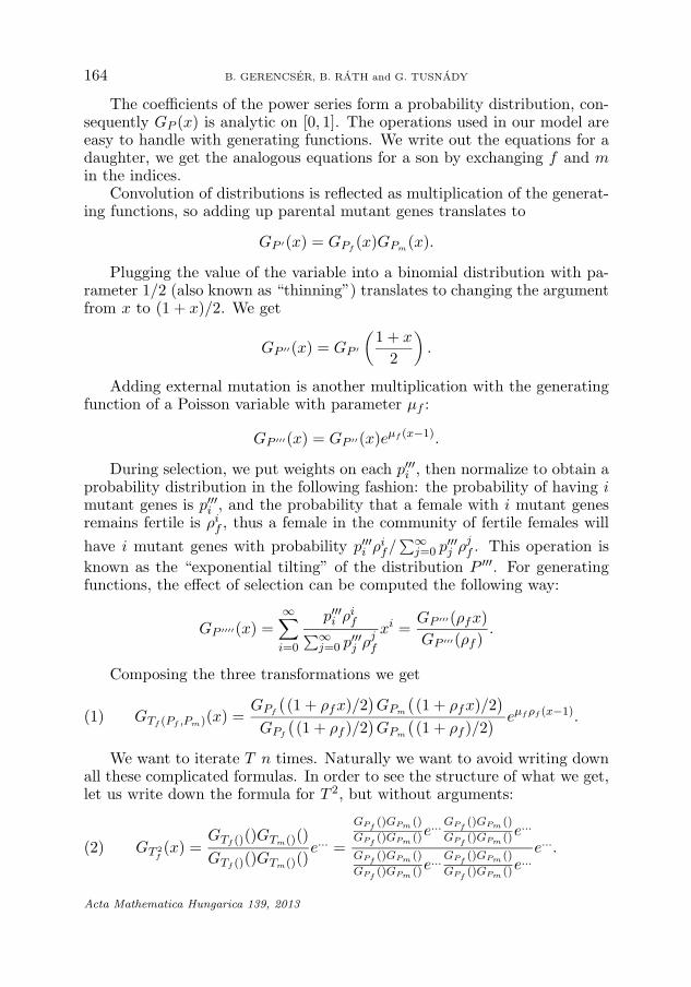
The coefficients of the power series form a probability distribution, con-sequently GP (x) is analytic on [0, 1]. The operations used in our model areeasy to handle with generating functions. We write out the equations for adaughter, we get the analogous equations for a son by exchanging f and min the indices.

Convolution of distributions is reflected as multiplication of the generat-ing functions, so adding up parental mutant genes translates to

GP ′ (x) = GPf(x)GPm

(x).

Plugging the value of the variable into a binomial distribution with pa-rameter 1/2 (also known as “thinning”) translates to changing the argumentfrom x to (1 + x)/2. We get

GP ′ ′ (x) = GP ′

(1 + x

2

).

Adding external mutation is another multiplication with the generatingfunction of a Poisson variable with parameter μf :

GP ′ ′ ′ (x) = GP ′ ′ (x)eμf (x−1).

During selection, we put weights on each p′ ′ ′i , then normalize to obtain a

probability distribution in the following fashion: the probability of having imutant genes is p′ ′ ′

i , and the probability that a female with i mutant genesremains fertile is ρi

f , thus a female in the community of fertile females willhave i mutant genes with probability p′ ′ ′

i ρif/

∑∞j=0 p′ ′ ′

j ρjf . This operation is

known as the “exponential tilting” of the distribution P ′ ′ ′. For generatingfunctions, the effect of selection can be computed the following way:

GP ′ ′ ′ ′ (x) =∞∑

i=0

p′ ′ ′i ρi

f∑∞

j=0 p′ ′ ′j ρj

f

xi =GP ′ ′ ′ (ρfx)GP ′ ′ ′ (ρf )

.

Composing the three transformations we get

(1) GTf (Pf ,Pm)(x) =GPf

((1 + ρfx)/2

)GPm

((1 + ρfx)/2

)

GPf

((1 + ρf )/2

)GPm

((1 + ρf )/2

) eμf ρf (x−1).

We want to iterate T n times. Naturally we want to avoid writing downall these complicated formulas. In order to see the structure of what we get,let us write down the formula for T 2, but without arguments:

(2) GT 2f(x) =

GTf ()()GTm()()GTf ()()GTm()()

e... =

GPf()GPm ()

GPf()GPm ()e

... GPf()GPm ()

GPf()GPm ()e

...

GPf()GPm ()

GPf()GPm ()e

... GPf()GPm ()

GPf()GPm ()e

...e....



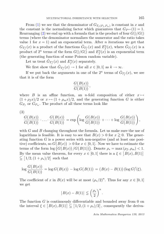
From (1) we see that the denominator of GTf (Pf ,Pm) is constant in x andthe constant is the normalizing factor which guarantees that GP ′ ′ ′ ′ (1) = 1.Rearranging (2) we end up with a formula that is the product of four G()/G()terms (where the denominator normalizes the numerator and the ratio takesvalue 1 for x = 1) and an exponential term. After n iterations we get thatGT n

f(x) is a product of the functions GT n

f(x) and En

f (x), where GT nf(x) is a

product of 2n terms of the form G()/G() and Enf (x) is an exponential term

(the generating function of some Poisson random variable).Let us treat GT n

f(x) and En

f (x) separately.We first show that GT n

f(x) → 1 for all x ∈ [0, 1] as k → ∞.

If we put back the arguments in one of the 2n terms of GT nf(x), we see

that it is of the form

G(B(x)

)

G(B(1)

) ,

where B is an affine function, an n-fold composition of either x �→(1 + ρfx)/2 or x �→ (1 + ρmx)/2, and the generating function G is eitherGPf

or GPm. The product of all these terms look like

G(B(x)

)

G(B(1)

) · . . . · G(B(x)

)

G(B(1)

) = exp

(log

G(B(x)

)

G(B(1)

) + · · · + logG

(B(x)

)

G(B(1)

))

,

(3)

with G and B changing throughout the formula. Let us make sure the use oflogarithms is feasible. It is easy to see that B(x) > 0 for x � 0. The gener-ating function G is a power series with non-negative (and at least one posi-tive) coefficients, so G

(B(x)

)> 0 for x ∈ [0, 1]. Now we have to estimate the

terms of the form log (G(B(x)

)/G

(B(1)

)). Denote ρ∗ = max (ρf , ρm) < 1.

By the mean value theorem, for every x ∈ [0, 1] there is a ξ ∈[B(x), B(1)

]

�[1/2, (1 + ρ∗)/2

]such that

logG

(B(x)

)

G(B(1)

) = log G(B(x)

)− log G

(B(1)

)=

(B(x) − B(1)

)(log G)′(ξ).

The coefficient of x in B(x) will be at most (ρ∗/2)n. Thus for any x ∈ [0, 1]we get

∣∣B(x) − B(1)∣∣ �

(ρ∗2

)n

.

The function G is continuously differentiable and bounded away from 0 onthe interval ξ ∈

[B(x), B(1)

]�

[1/2, (1 + ρ∗)/2

], consequently the deriva-



tive of the logarithm can be bounded in absolute value by some C. In theend we get

∣∣∣∣∣logG

(B(x)

)

G(B(1)

)∣∣∣∣∣ < C

(ρ∗2

)n

.

Adding up 2n of such terms gives the bound∣∣∣∣∣log

G(B(x)

)

G(B(1)

) + · · · + logG

(B(x)

)

G(B(1)

)∣∣∣∣∣ � Cρn

∗ .

This tends to 0 for all x ∈ [0, 1], thus the product on the left-hand side of (3)converges to 1 as n → ∞. Observe that the exponential term in En

f (x) doesnot depend on the initial distributions Pf , Pm. Thus we have just shownthat the only part depending on the initial distributions vanishes. Con-sequently the convergence and the potential limit does not depend on theinitial distributions.

It is now enough to show a pair of distributions satisfying

(Pf , Pm) =(Tf (Pf , Pm), Tf (Pf , Pm)

),

as the previous reasoning ensures that the trivial convergence of this caseimplies convergence for any initial generating functions to this fixed point.We search among Poisson distributions because this family is closed for allthe transformations we use. The pair (λf , λm) is invariant exactly when

λf =(

λf + λm

2+ μf

)ρf , λm =

(λf + λm

2+ μm

)ρm.

Taking the average of the two equations results in a simple expression for(λf +λm)/2, plugging it back gives us the parameters stated in the theorem.

To conclude we use the fact that the convergence of a sequence of gen-erating functions to a generating function on [0, 1] implies the convergenceof the corresponding probability distributions (see e.g. Mukherjea et al. [5]).�

We should note that the proof strongly relies on the specific choice ofselection which we can conveniently handle using generating functions. Aswe mentioned in the introduction, it makes sense to consider different func-tions determining the risk based on the mutant gene count. However, it isunclear how one should modify the proof to resolve the alternative cases.

4. Theoretical disorder probabilities

From the previous section we learn that it makes sense to assume thepopulation to be in the stationary state. It is easy to check that the num-



ber of mutant genes a newborn has follows a Poisson distribution with thefollowing parameters depending on the gender:

λf + λm

2+ μf =

λf

ρf,

λf + λm

2+ μm =

λm

ρm.

Consequently his/her probability of being healthy is

pf = exp

(λf

Δf − 1ρf

), pm = exp

(λm

Δm − 1ρm

).

Similarly, the probability of being fertile is

pf = exp

(λf

ρf − 1ρf

), pm = exp

(λm

ρm − 1ρm

).

However, if we look at a family tree at once, we see a complex multidimen-sional joint distribution. We want to answer simple questions like “Whatis the (conditional) probability of an aunt of a malformed child being af-fected?”.

We claim that we can get a closed form expression on any reasonableconditional probabilities like above. The resulting formulas often becomeenormous, but there is a way to derive them with reasonable effort.

We would like a general iterative computational scheme that can be usedfor most cases. The idea is to draw a graph of the family tree, transform itto simpler graphs while building the formula for the probability.

We include the possible dependence on the gender of the patient. There-fore the parameters we have are

μf , μm, ρf , ρm,Δf ,Δm.

The parameters of the stationary distributions are

λf =ρfρm(μm − μf ) + 2ρfμf

2 − ρf − ρm, λm =

ρfρm(μf − μm) + 2ρmμm

2 − ρf − ρm.

From now on to reduce the number of formulas, we use x, y, . . . for onegender or another, thus μx or λy is the parameter corresponding to the ap-propriate gender. In addition we use x′ for the gender different from x.

4.1. Representing graphs. First, let us visualize the situation. Wemay draw a family tree with some additional information.

We use Fig. 1 as an example. Suppose x = m, y = m, z = f for a mo-ment. The circles in the graph represent members or couples of the family.



Fig. 1: Healthy boy and aunt (or similar)

In this case B is the male patient we start at, A is the mother, C is the fa-ther. D represents the paternal grandparents together. We do not separatethem as we use only the joint genetic information of them. The last memberE is an aunt.

The genetic information moves in the following way. Each line representsa parental relation, so each gene is inherited downwards independently withprobability 1/2. The values above the circles show where additional mutantgenes enter the system. We always mean a Poisson random variable withthe parameter being the value indicated. These are obviously μu for mostpeople, and λu or λf + λm for the people or couples we start with.

The event we want to investigate is coded in the values below the circles.They show a per-gene probability for mutant genes that the actual personcomplies with the event. In the figure above we have Δu in two positionswhich means we want the patient and the aunt (or uncle) to be healthy. Theρy under C is an implied restriction, as we need the father (or mother) tobe fertile for the graph to be valid. Some places have no value indicated, wehave no restriction there, we may also write 1 to these places.

This way we can only express events requiring some to be healthy, someto be fertile, but these are the ones that are easy to directly compute. By ba-sic inclusion-exclusion formulas we can also handle events about some beingaffected or infertile. To compute conditional probabilities we simply need todivide two of such probabilities.

Now let us get into computational details to work through our plan.

4.2. Processing graphs. We can handle the simplest graph possible:

Fig. 2: Basic graph



The probability of the event described by this basic graph is

∞∑

i=0

ηi

i!e−ηαi = exp

(η(α − 1)

).

We introduce a few graph operations so we can transform complex graphsinto simpler ones. Observe that if a final descendant receives mutant genesfrom multiple sources, they pose independent threats, so we can split thegraph as pictured below.

Fig. 3: Splitting a graph

The other operation we use is to merge a child to the parent. Considerthe following setting:

Fig. 4: Parent and child

We condition on the number of mutant genes the parent has, supposeit is c. Then the distribution of mutant genes the child inherits follows aBinom (c, 1/2) distribution. So the probability that the child behaves ac-cording to the event is

c∑

i=0

(c

i

) (12

)c

αi =(

1 + α

2

)c

.

This is an exponential term in c, so we do not change the overall probabilityof the event if we omit the child but multiply the risk factor of the parentby (α + 1)/2.

It is easy to see that any acyclic family tree can be reduced to containonly a few copies of the simplest one-node graph.



Fig. 5: Merging a child

4.3. Siblings. Let us start with the simplest case, computing condi-tional probabilities for first order relatives. We want to find out the con-ditional probability of a sibling of a malformed child being affected. Fig. 6shows the graph for the sibling.

Fig. 6: Healthy patient and sibling

Let us use the notation scheme pAC , this stands for the probability of Abeing affected by the risk and C not (and we do not count on others). Thismeans the conditional probability qS we need is

qS =pAC

pA

.

Using inclusion-exclusion formulas we have

pAC = 1 − pA − pC + pAC , pA = 1 − pA.

The method in the previous section allows us to compute these prob-abilities. When computing pA, we replace the risk of C by 1. The graphdecomposition is shown in Fig. 7. By symmetry we can calculate pC analo-gously. We show the graph decomposition for computing pAC in Fig. 8.

We do not aim for the simplest expressions, we rather leave it in a formthat is easier to check.

pA = exp((

μx +λf + λm

2

)(Δx − 1)

),

pC = exp((

μy +λf + λm

2

)(Δy − 1)

),



Fig. 7: Graph decomposition to compute pA

Fig. 8: Graph decomposition to compute pAC

pAC = exp(

μx(Δx − 1) + μy(Δy − 1) +λm + λf

4((Δx + 1)(Δy + 1) − 4

)).

In case of complete selection and symmetric gender roles, i.e.

Δm = Δf = ρm = ρf = ρ, λf = λm = λ, and μm = μf = μ,

the conditional probability qS is

qS = 2 − 1 − e−t

1 − e−μ,

where

t = 2μ(1 − 1

4ρ(1 − ρ)

),

and ρ = λλ+μ . Surprisingly qs depends on ρ through the term ρ(1 − ρ). In

this case the population prevalence simplifies to

pA = 1 − exp((λ + μ)(ρ − 1)

)= 1 − exp

(λ − (λ + μ)

)= 1 − exp (−μ).

thus ρ is a free parameter and qS is a symmetric function of ρ regarding theswap ρ = 1 − ρ. We are curious whether there is a direct explanation forthis symmetry. When μ is small and ρ = 1

2 , then λ = μ and a bad gene israre. An affected child gets a bad gene fifty-fifty either from mutation orfrom one of his/her parents. In the second case the sibling gets the bad genefrom the affected parent with half probability and the bad gene is expressedagain with probability half. Accordingly qS is close to 1

8 . We shall refer tothis parametrization as standard model.



4.4. Parent. Next we calculate the conditional probability for a par-ent being affected, which is also fairly simple. See Fig. 9 for the describinggraph. The only novelty is the Δy/ρy risk of the parent. It is easy to see thatthis is the risk of not being affected by the disorder conditioned on beingfertile.

Fig. 9: Healthy patient and parent

qP =pBC

pB

=1 − pB − pC + pBC

1 − pB,

pB = exp((

μx +λf + λm

2

)(Δx − 1)

),

pC = exp

(λy

(Δy

ρy− 1

)),

pBC = exp

((μx +

λy′

2

)(Δx − 1) + λy

(Δy

ρy

(Δx + 1

2

)− 1

)).

In the standard model, when ρf = ρm = Δf = Δm = 1/2 and μf = μm

is small, we get qP = 0. This is rather clear because this special case impliescomplete selection.

4.5. Grandparent. Let us move on to higher order relatives, startingwith grandparents. Fig. 10 shows the actual graph to be processed. Theconditional probability can be expressed as

qG =pBCD

pBC

=pC − pBC − pCD + pBCD

pC − pBC,

pC = exp((

μy +λf + λm

2

)(ρy − 1)

),

pBC = exp((

μx +λy′

2

)(Δx − 1) +

(μy +

λf + λm

2

) (ρy

Δx + 12

− 1))

,



Fig. 10: Healthy patient and grandparent

pCD = exp((

μy +λz′

2

)(ρy − 1) + λz

(Δz

ρz

(ρy + 1

2

)− 1

)),

pBCD = exp

⎛

⎝(

μx +λy′

2

)(Δx − 1) +

(μy +

λz′

2

) (ρy

Δx + 12

− 1)

+ λz

(Δz

ρz

(ρy

Δx+12 + 12

)− 1

) ⎞

⎠.

In the standard model we get qG = 0 as we expect because of the com-plete selection.

4.6. Aunt and uncle. Let us turn to investigating aunts and uncles.We use Fig. 1 for the calculation. The conditional probability can be ex-pressed as

qA =pBCE

pBC

=pC − pBC − pCE + pBCE

pC − pBC.

We can compute the occurring probabilities as before. Without going intodetails, we get

pC = exp((

μy +λf + λm

2

)(ρy − 1)

),

pBC = exp((

λy′

2+ μx

)(Δx − 1) +

(μy +

λf + λm

2

) (ρy

Δx + 12

− 1))

,

pCE = exp(

μy(ρy − 1) + μz(Δz − 1)

+ (λf + λm)(

(ρy + 1)(Δz + 1)4

− 1))

,



pBCE = exp

⎛

⎝μz(Δz − 1) +(

μx +λy′

2

)(Δx − 1) + μy

(ρy

Δx + 12

− 1)

+λf + λm

4

((ρy

Δx + 12

+ 1)

(Δz + 1) − 4)⎞

⎠.

Plugging these back gives us the conditional probability we were lookingfor.

In the standard model the number of halving factors is 5:– the affected child might get the bad gene by mutation,– or by the parent out of link to aunt-uncle,– the parent in the link to aunt-uncle might get the bad gene by muta-

tion,– the grandparents need not to pass it to another child,– who needs not to express the malformation.We get qA = 1/32 as well by using the expressions above for the standard

model.

4.7. Cousin. To compute the analogous conditional probability forcousins, we will use Fig. 11 below.

Fig. 11: Healthy patient and cousin

Using the same method, we want to compute

qC =pBCEF

pBCE

=pCE − pBCE − pCEF + pBCEF

pCE − pBCE= 1 − pCEF − pBCEF

pCE − pBCE.

For the individual probabilities in this setting we get

pCE = exp(

μy(ρy − 1) + μz(ρz − 1) +λf + λm

4((ρy + 1)(ρz + 1) − 4

)),



pBCE = exp

⎛

⎝(

μx +λy′

2

)(Δx − 1) + μz(ρz − 1) + μy

(ρy

Δx + 12

− 1)

+λm + λf

4

((ρy

Δx + 12

+ 1)

(ρz + 1) − 4)⎞

⎠,

pCEF = exp

⎛

⎝(

μv +λz′

2

)(Δv − 1) + μy(ρy − 1) + μz

(ρz

Δv + 12

− 1)

+λm + λf

4

((ρz

Δv + 12

+ 1)

(ρy + 1) − 4)⎞

⎠,

pBCEF = exp

⎛

⎝(

μx +λy′

2

)(Δx − 1) +

(μv +

λz′

2

)(Δv − 1)

+ μy

(ρy

Δx + 12

− 1)

+ μz

(ρz

Δv + 12

− 1)

+λf + λm

4

((ρy

Δx + 12

+ 1) (

ρzΔv + 1

2+ 1

)− 4

)⎞

⎠.

These are rather cumbersome formulas, but in the standard model, weget qC = 1/124. At first this is a bit surprising, because by counting thenumber of halving factors as before, we get 1/27 = 1/128. We should notethat checking a cousin for the disorder implies he is already born, that is,his parents are fertile. Conditioning on this accounts for a division by 31/32which brings us to the correct value.

5. Validation of the model

It is an important milestone to have a model which we can handle, westill have to check how well does it follow biological principles and how doesit fit the population. Let us recall the notations introduced in Section 4:

p = P (subject is affected), qS = P (sibling is affected | subject is affected).

The initial requirement for a model with inheritance is to have high condi-tional probabilities for first order relatives, in other words qS � p. To test



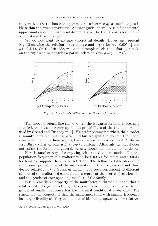
this, we will try to choose the parameters to increase qS as much as possi-ble within the given constraints. Another guideline we use is a fundamentalapproximation on multifactorial disorders given by the Edwards formula [2]which states that qS ≈ √

p.We do not want to go into theoretical details, let us just present

Fig. 12 showing the relation between log p and log qS for μ ∈ [0.005, 1] andρ ∈ [0.5, 1). On the left side, we assume complete selection, that is, ρ = Δ,on the right side we consider a partial selection with ρ = (1 + Δ)/2.

Fig. 12: Model probabilities and the Edwards formula

The upper diagonal line shows where the Edwards formula is preciselysatisfied, the lower one corresponds to probabilities of the Gaussian modelused by Czeizel and Tusnady in [1]. We prefer parameters where the disorderis mainly inherited, that is, λ � μ. Thus we split the domain the modelsweeps through into three regions, the values we can reach while λ � 10μ, orjust 10μ > λ � μ, or only μ � λ (top to bottom). Although the model doesnot satisfy the formula in general, we may choose the parameters to do so.

Here is another way of comparing with the Gaussian model. Let thepopulation frequency of a malformation be 0.00071 for males and 0.00317for females, suppose there is no selection. The following table shows theconditional probabilities of the malformation in the first, second and thirddegree relatives in the Gaussian model. The rows correspond to differentgenders of the malformed child, columns represent the degree of relationshipand the gender of corresponding member of the family.

It is a remarkable property of the multifactorial threshold model that arelative with the gender of larger frequency of a malformed child with thegender of smaller frequency has the maximal conditional probability. Thereason for the property is that the malformed child with smaller frequencyhas larger liability shifting the liability of his family upwards. The relatives



I I II II III IIIM F M F M F

M 0.0393 0.1149 0.0076 0.0276 0.0024 0.0195F 0.0232 0.0749 0.0055 0.0204 0.0014 0.0087

Table 1: Conditional probabilities in the Gaussian model without selection

with gender of larger frequency is evaluated with a smaller threshold whichresults in the mentioned property. The following table gives the conditionalprobabilities for the case with complete selection for the Gaussian model.


M 0.0365 0.1025 0.0085 0.0255 0.0032 0.0113F 0.0242 0.0739 0.0063 0.0234 0.0020 0.0088

Table 2: Conditional probabilities in the Gaussian model with complete selection

We compare these values with those coming from the Poisson model. Weassume μf = μm, and use the remaining degree of freedom to get the high-est conditional probabilities as mentioned in the beginning of this section.Having no selection means ρf = ρm = 1 but in this case we cannot applyTheorem 1. We rather choose ρf = ρm = 1 − ε for some small ε > 0 to allowonly negligible selection, but stay within the conditions of Theorem 1.


M 0.1124 0.5015 0.0566 0.2523 0.1475 0.1722F 0.1123 0.5012 0.0565 0.2521 0.1473 0.1721

Table 3: Conditional probabilities in the Poisson model with negligible selection

With complete selection:


M 0.0452 0.2017 0.0135 0.0603 0.0342 0.0418F 0.0452 0.2015 0.0135 0.0602 0.0342 0.0418

Table 4: Conditional probabilities in the Poisson model with complete selection

The reassuring fact we see is that we can set the conditional probabilitieseven higher than in the Gaussian model while leaving population probabili-ties unchanged.



Fig. 13: Model family

Next, we perform a Monte Carlo simulation on a model family given inFig. 13. We fix that A2, A4, A6, A8, B6 are women, A1, A3, A5, A7, B3are men. The following numbers in Table 5 are probabilities conditionedon C5 having the malformation. We generated a large number of familiesstarting from A1–A8 and only selected those where C5 was born and hadthe malformation. This explains the zeros in the first lines as they are allparents and consequently they are healthy. This does not hold for B1 as weallow him/her to be infertile thus C1 might not be born.

Gender ofrelative index A1 A2 A3 A4 A5 A6 A7 A8

M M 0.00000 0.00000 0.00000 0.00000 0.00000 0.00000 0.00000 0.00000M F 0.00000 0.00000 0.00000 0.00000 0.00000 0.00000 0.00000 0.00000F M 0.00000 0.00000 0.00000 0.00000 0.00000 0.00000 0.00000 0.00000F F 0.00000 0.00000 0.00000 0.00000 0.00000 0.00000 0.00000 0.00000

B1 B2 B3 B4 B5 B6 B7 B8

M M 0.00100 0.00071 0.00000 0.01853 0.00752 0.00000 0.00077 0.00077M F 0.00079 0.00064 0.00000 0.01890 0.00887 0.00000 0.00069 0.00068F M 0.00295 0.00305 0.00000 0.08952 0.03948 0.00000 0.00288 0.00293F F 0.00334 0.00290 0.00000 0.08458 0.03906 0.00000 0.00306 0.00310

C1 C2 C3 C4 C5 C6 C7 C8

M M 0.00701 0.00684 0.00813 0.04489 1.00000 0.04284 0.00221 0.00290M F 0.00706 0.00657 0.00717 0.04408 0.00000 0.04392 0.00310 0.00312F M 0.03072 0.03130 0.03076 0.18805 0.00000 0.19658 0.01346 0.01445F F 0.02944 0.02999 0.02988 0.19319 1.00000 0.19074 0.01485 0.01411

Table 5: Conditional probabilities in the Poisson model with complete selection

The gender of the affected child has seemingly no effect beyond random-ness. One explanation for this phenomena is that in case of rare malfor-mations the only effect that the affected child might cause is that he/shehas a bad gene which is independent of gender differences. Using this setupalso allows us to numerically compute more elaborate conditional and jointprobabilities.


MULTIFACTORIAL INHERITANCE WITH SELECTION 179pop

table

no

page

type

of

Sex

freq

No

Fath

erM

oth

erB

roth

erSis

ter

ICC

A1000

mM

Mm

MM

mM

Mm

MM

20

71

ASB

Boy

2.2

2134

134

00.0

134

00.0

102

12.3

86

22.8

Gir

l3.5

9309

309

00.0

309

00.0

210

54.0

177

45.3

30

96

CL(P

)B

oy1.3

3369

304

33.6

304

56.9

143

16

5.7

121

03.9

Gir

l0.7

7200

161

32.4

166

74.9

80

14.4

89

44.1

35

114

CH

PS

Boy

2.1

8112

112

10.5

112

21.4

48

22.0

38

21.1

Gir

l0.6

936

36

00.5

36

11.4

15

31.3

10

00.8

43

134

VSD

Boy

1.7

2180

180

10.4

180

21.8

121

02.6

109

22.1

Gir

l1.4

1197

197

00.5

197

32.3

96

22.2

81

11.6

56

166

CD

H-B

BB

oy11.9

6422

422

76.3

422

20

32.2

125

20

22.6

126

20

32.9

Gir

l39

1345

1345

96.4

1345

46

32.7

421

29

34.3

398

79

72.4

57

170

CD

H-C

BB

oy8.1

375

75

10.4

75

27.3

22

24.8

21

77.0

Gir

l50.5

7304

304

00.4

304

13

7.3

89

66.8

75

14

17.0

69

195

ST

EV

Boy

1.6

5118

118

42.7

118

31.5

61

42.6

60

12.2

Gir

l0.8

256

56

12.5

56

01.3

29

22.0

30

31.9

Pate

rnal

Mate

rnal

Pate

rnal

Mate

rnal

cousi

ns

uncl

eaunt

uncl

eaunt

Boy

Gir

lB

oyG

irl

mM

Mm

MM

mM

Mm

MM

mM

Mm

MM

mM

Mm

MM

ASB

Boy

306

04.5

260

16.6

290

14.3

302

07.6

387

05.7

447

011.3

283

04.2

307

17.8

Gir

l505

17.4

512

012.9

497

37.3

534

013.5

850

212.6

785

219.9

606

39.0

621

315.8

CL(P

)B

oy283

33.6

307

32.3

383

05.5

366

23.3

362

14.6

374

02.8

365

14.7

387

22.9

Gir

l163

12.1

198

11.5

172

32.7

200

22.0

174

02.2

219

11.6

156

22.0

166

01.3

CH

PS

Boy

153

03.1

146

01.0

180

13.6

166

11.2

130

22.6

136

00.9

154

13.0

144

11.0

Gir

l42

00.9

33

00.3

42

00.9

39

00.4

31

00.6

28

00.2

45

10.9

31

00.2

VSD

Boy

272

34.3

225

53.0

214

33.4

214

02.9

261

14.1

248

23.3

192

03.0

181

12.4

Gir

l208

33.3

168

12.2

188

43.0

209

32.8

239

03.8

168

12.3

175

02.8

174

02.3

CD

H-B

BB

oy675

229.7

609

11

92.7

561

729.4

600

895.3

602

429.3

666

58

103.8

544

726.6

544

35

84.9

Gir

l1676

771.5

1473

25

222.6

1530

569.4

1607

55

246.2

1643

50

79.7

1637

128

255.0

1333

52

64.8

1282

172

199.8

CD

H-C

BB

oy60

02.4

45

09.0

60

03.1

45

09.4

42

12.0

44

69.0

42

12.0

45

69.2

Gir

l273

210.5

263

652.2

273

111.3

263

652.8

197

49.2

203

12

41.5

197

49.2

204

12

41.7

ST

EV

Boy

140

02.3

161

21.5

141

02.2

151

11.3

131

12.0

130

01.1

148

22.3

121

01.0

Gir

l86

21.5

70

00.7

69

01.1

84

00.8

72

01.1

67

00.6

55

20.8

55

20.5

Tabl

e6:

Num

ber

ofre

lative

s(m

),num

ber

ofaffec

ted

rela

tive

sin

Hunga

rian

data

(M),

expe

cted

num

ber

ofaffec

ted

rela

tive

sfo

rth

e

Poisso

nm

odel

(M)



Another way to qualify the power of the Poisson model is to check itsgoodness-of-fit on the Hungarian data. In Table 6 we show the Poissonmodel fitted to 7 different data sets. The population data were gatheredand published by Czeizel and Tusnady [1].

In Table 7 we present the goodness-of-fit values for the same data. Wecalculate the weighted average of the divergences for each relative. Fromanother viewpoint, this is the normalized log-likelihood loss when changingreal frequencies to the predicted probabilities.

disorderGOF for GOF for

all relatives first order relatives

ASB 0.012189 0.000615CLP 0.005341 0.008989

CHPS 0.007234 0.007099VSD 0.005122 0.003212

CDH-BB 0.031767 0.002309CDH-CB 0.050819 0.007456STEV 0.007865 0.007432

Table 7: Goodness-of-fit of the Poisson model to Hungarian data

Finally let us present the parameter values for the best fit in Table 8.

disorder μm μf ρm ρf Δm Δf λm λf

ASB 0.015 0.026 0.018 0.010 0.018 0.010 0.00027 0.00026CLP 0.012 0.0075 0.019 0.143 5.0e-14 0.085 0.00024 0.0012

CHPS 0.020 0.006 0.069 0.078 0.061 0.00052 0.0015 0.00052VSD 0.016 0.013 0.0040 0.023 1.7e-17 1.3e-17 6.2e-5 0.00031

CDH-BB 0.036 0.175 0.028 0.142 3.4e-32 0.105 0.0014 0.027CDH-CB 0.030 0.237 0.010 0.137 6.5e-16 0.102 0.00050 0.035STEV 0.015 0.0073 0.091 0.048 0.047 1.2e-14 0.0015 0.00039

Table 8: Parameters of the Poisson model for Hungarian data

We present in Table 6 the observed occurrences M together with theirexpected numbers M because these pairs offer the most plausible insightinto goodness-of-fit. As it is transparent the majority of M -s are close to Mwith the exception of third degree relatives.

Accordingly, the first kind errors given in Table 7 are encouragingly smallwith the only exception of CDH-CB for all relatives. This body of Hungarianfamily data is less reliable because the lack of sound agreement of diagnosisof congenital dislocation of hip for different generations in XXth centurycountryside in Hungary.

Honestly we were quite shocked by the extremely small frequencies inTable 8. Only after understanding the dynamics of the standard model can



we state that the Poisson model offers rather acceptable fit for Hungariandata. The only question remained is the relation of Poisson model withextremely low presence of bad genes in population with the Mendelian modelwith dominance where the probability of expression of the malformation isaround 1/2.

6. Conclusion

Let us denote by bk the probability that a fertile person has k bad genes.Then the distribution of bad genes in the next generation has the form

ck =∑

i=1

∑

j=1

H(i, j, k)bibj ,

where the kernel H is determined by biology. As it was shown in Tusnady [7]with an example, bilinear transformations of this form may be chaotic evenif all the elements of H are positive. In the paper Hatvani et al. [3], thecase of continuous time is investigated. It is shown that the stability of apositive bilinear operator is not ensured by the positivity of the kernel, butno example was found having chaotic attractor.

The form of selection investigated in the present paper is fortunate andensures stability. The goodness-of-fit to population data is acceptable, theonly problems are the extraordinarily small values for the parameter λ. Thismeans that the number of bad genes is usually zero, and the appearanceof a single bad gene causes the malformation or selection. Still, the low λdoes not necessarily mean that the number of genes involved is small. Aswe mentioned in the introduction, we qualify our solution partial. It is afirst acceptable solution for the problem resulting in a sound and practicallyapplicable model. Still, the stability of the models with threshold remainsopen.

In a certain way the Poisson setup is richer than the Gaussian one as theexpression of the malformation is randomized. The situation of this modelis close to dominant Mendelian inheritance with restricted expression. If theprobability of the expression depends on the gender then the situation israther complex. In the standard model the conditional probabilities resem-ble the formulas of Gaussian correlations. However, when allowing genderdifferences in the parameters the Poisson model becomes richer: conditionalprobabilities (of a relative being affected when the child is affected) showstronger gender dependence in the Poisson model than in the Gaussian one.Now we are facing the question, whether the Poisson model incorporatedwith environmental effects offer a substantially better goodness-of-fit thanthe Gaussian one.


182 B. GERENCSER, B. RATH and G. TUSNADY: MULTIFACTORIAL INHERITANCE . . .

Acknowledgements. We would like to express our thanks to VilloCsiszar for her helpful and inspiring comments. We would also like to thankGyorgy Michaletzky for his support on performing the numerical investiga-tions of the models.

We are grateful to the anonymous referee for his/her thorough and de-tailed review which we believe helped us to significantly improve the clarityand the quality of this paper.

References

[1] E. Czeizel and G. Tusnady, Aetiological Studies of Isolated Common Congenital Ab-normalities in Hungary, Akademiai Kiado (Budapest, 1984).

[2] J. Edwards, The genetic basis of common disease, Am. J. Med., 34 (1963), 627–638.[3] L. Hatvani, F. Tookos and G. Tusnady, A mutation-selection-recombination model in

population genetics, Dyn. Syst. Appl., 18 (2009), 335–362.[4] S. Karlin, Models of multifactorial inheritance: I, multivariate formulations and basic

convergence results* 1, Theor. Popul. Biol., 15 (1979), 308–355.[5] A. Mukherjea, M. Rao and S. Suen, A note on moment generating functions, Stat.

Probab. Lett., 76 (2006), 1185–1189.[6] K. Sankaranarayanan, N. Yasuda, R. Chakraborty, G. Tusnady and A. Czeizel, Ionizing

radiation and genetic risks. V. Multifactorial diseases: A review of epidemio-logical and genetic aspects of congenital abnormalities in man and of modelson maintenance of quantitative traits in populations, Mutat. Res., Rev. Genet.Toxicol., 317 (1994), 1–23.

[7] G. Tusnady, Mutation and selection, Magy. Tud., 7 (1997), 792–805 (in Hungarian).


Documents

Multifactorial inheritance with selection