Acknowledgments

Our interest in fractal modeling was spurred during our graduate yearsat Yale by conversations with Benoıt Mandelbrot, the father of fractalgeometry. This interaction evolved into the collaborative development ofthe Multifractal Model of Asset Returns (MMAR), which was originallycirculated in three Cowles Foundation Discussion Papers (Calvet, Fisher,and Mandelbrot, 1997). The core of this work was eventually published inthe Review of Economics and Statistics in 2002.

In order to develop practical applications such as volatility forecast-ing and pricing, we then independently developed a Markov model withmultifrequency characteristics, which we called the Markov-switching mul-tifractal (MSM). We first presented MSM, both in discrete and continuoustime, at the 1999 National Bureau of Economic Research Summer Insti-tute organized by Francis Diebold and Kenneth West, and published thiswork in the corresponding special issue of Journal of Econometrics. MSMstimulated a flow of subsequent research on the econometric and pricingapplications of multifrequency volatility risk, which we are now presentingin this book.

Many of the chapters draw heavily from earlier publications in academicjournals. The presentation of discrete-time MSM in Chapter 3 follows “Howto Forecast Long-Run Volatility: Regime-Switching and the Estimation ofMultifractal Processes,”presented in 2002 at the CIRANO Conference onExtremal Events in Finance, organized by Rene Garcia and Eric Renault,and published in the Journal of Financial Econometrics. Multivariate MSMin Chapter 4 was presented in September 2003 at the Penn-IGIER confer-ence organized by Francis Diebold and Carlo Favero, and appeared in theJournal of Econometrics under the title “Volatility Comovement: A Multi-frequency Approach.” This article is joint with Samuel Thompson, a formerHarvard colleague now at Arrowstreet Capital, L.P.

Chapters 6 and 8 follow the Review of Economics and Statistics article“Multifractality in Asset Returns: Theory and Evidence.” The discussionof continuous-time MSM in Chapter 7 is a thoroughly revised version ofthe Journal of Econometrics publication “Forecasting Multifractal Volatil-ity.” Chapter 9 is based on “Multifrequency News and Stock Returns,”which was first presented at Wharton in March 2003 and appeared in theJournal of Financial Economics. Chapter 10 borrows from “MultifrequencyJump-Diffusions: An Equilibrium Approach,” which was prepared for the2005 NSF/CEME Conference in Honor of Gerard Debreu organized byChris Shannon at UC Berkeley and was published in Journal of Mathe-matical Economics. We have liberally added and subtracted from theseearlier papers in order to produce a coherent book.

x Acknowledgments

We would like to thank many colleagues and friends who have contributedto the development of the multifrequency research presented in this book.We are especially grateful to John Campbell and Francis Diebold for theircontinued support over the past decade. During our graduate years, the fac-ulty of Yale University gave us insightful feedback, and John Geanakoplos,Peter Phillips, Robert Shiller and Christopher Sims in particular providedus with invaluable help. We thank Samuel B. Thompson for the fruitful col-laboration on which Chapter 4 is based. We also acknowledge the generoushelp of Karim Abadir, Andrew Abel, Torben Andersen, Donald Andrews,Tim Bollerslev, Michael Brandt, Andrea Buraschi, Bernard Cornet, WalterDistaso, Darrell Duffie, Robert Engle, Francesco Franzoni, Rene Garcia,William Goetzmann, James Hamilton, Lars Hansen, Oliver Hart, JeanJacod, Guido Kuersteiner, Guy Laroque, Oliver Linton, Eric Maskin, NourMeddahi, Andrew Metrick, Marcelo Moreira, Jacques Olivier, Jack Porter,Stephen Ross, Jose Scheinkman, Neil Shephard, Bruno Solnik, RobertStambaugh, Jeremy Stein, James Stock, Jessica Wachter, Kenneth West,Amir Yaron, Paolo Zaffaroni, Stanley Zin, and our current and formercolleagues at Harvard, HEC Paris, Imperial College London, New YorkUniversity, and the University of British Columbia.

We thank Karen Maloney, our editor at Elsevier, who encouraged usto write this book and displayed considerable enthusiasm throughout theduration of this project. We are also grateful to Roxana Boboc and MelindaRitchie for their patient assistance.

Last but not least, we thank our families for their love and kind supportwhile this work was under way. This book is dedicated to them.

Foreword

The study of financial markets has become one of the most active and pro-ductive empirical endeavors in the social sciences. A cynic, or a trainedeconomist, might say that the volume of financial research reflects the highprice that market participants are willing to pay for it, but there are alsodeep intellectual reasons for the interest in financial market data.

First, these data are abundant at all frequencies from tick-by-tick data atone extreme, to century-by-century data at the other, and across multiplecorrelated assets. Such data abundance is atypical in the social sciences,and it compensates to some degree for the fact that the data are generatedby the interactions of investors rather than by controlled experiments.

Second, the uncertainty that financial econometricians face when esti-mating their models is the same uncertainty that investors face when theytrade in asset markets and determine market prices. As Campbell, Lo,and MacKinlay (1997) express it, “The random fluctuations that requirethe use of statistical theory to estimate and test financial models are inti-mately related to the uncertainty on which those models are based.” Thisgives financial modelling a special relevance to market participants. Intel-lectually, it poses the challenge of building stochastic equilibrium modelsin which the second and higher moments of random shocks determine thefirst moments of asset returns.

As financial econometricians have explored the properties of asset returndata over the past 30 years, they have uncovered some fascinating regulari-ties. First, measured at high frequencies, the distribution of asset returns isvery far from normal; there is excess kurtosis, a strong tendency for returnsto stay either very close to the mean or far from it. Investors were forcefullyreminded of the non-normality of stock returns when stock prices crashedin October 1987, although the basic facts were already well established inthe academic literature.1 This non-normality diminishes when returns aremeasured over longer time intervals.

Second, conditioning information can be used to predict both first andsecond moments of asset returns. The predictability in first moments issubtle, as one would expect given the fundamental insight of the efficientmarkets hypothesis, that competition among investors ensures modest trad-ing profits so that most price variation is driven by the arrival of news. Thepredictability in second moments, on the other hand, is obvious even to a

1I vividly remember delivering a technical lecture on excess kurtosis at Princeton

during the morning of October 19, 1987. A student at the back of the room put up hishand and said “Professor Campbell, are you aware that the Dow is down 200 points?”I was not.

xii Foreword

casual observer. A vast literature on this phenomenon has documented thatconditional volatility can move suddenly but also varies persistently, so thattime-varying volatility is apparent both within the trading day and acrossdecades. Movements in conditional volatility often appear to be correlatedwith asset returns themselves.

A direct way to model changing second moments is to write down aprocess for the volatility of returns, conditional on past returns and possiblyother information available to an econometrician. In the early 1980’s RobertEngle followed this direct approach when he proposed the ARCH model.This seminal contribution was recognized in 2003 by the award to Engle ofthe Nobel Memorial Prize in Economic Sciences.

While the ARCH framework is a natural way to model changing volatil-ity, it does not offer an integrated explanation of return phenomena at dif-ferent frequencies. It explains high-frequency non-normality by exogenousnon-normal shocks, and persistence of volatility using a slowly decaying(fractionally integrated) volatility process. Each of these features must bechosen separately to match different aspects of financial market data.

An alternative approach, which has attracted interest in recent years, isto write down a process for a latent state variable that is not observableto the econometrician.2 The simplest version of this “stochastic volatil-ity” approach assumes that, conditional on the state variable, returns arenormally distributed with a volatility governed by the state variable, andthat the state variable follows a smooth autoregressive process. Since thestate variable is unobserved, returns are not in general normal conditionalon observed information, so in principle a smoothly evolving stochasticvolatility model can explain a wide variety of asset pricing phenomena. Inpractice, however, empirical analyses of stochastic volatility models findthat additional jumps are needed to fit the data: jumps in volatility, toaccommodate sudden changes in volatility, and jumps in prices, to gen-erate the extreme non-normality observed in high-frequency return data.Correlation between these jumps causes sudden movements in asset pricesto predict subsequent volatility (Duffie, Pan, and Singleton, 2000, Eraker;Johannes, and Polson, 2003).

Once stochastic volatility is allowed to jump, it becomes natural to con-sider a discrete-state regime-switching model of the sort introduced to theeconomics literature by Hamilton (1988, 1989). Regime-switching modelsare particularly appealing because they are tractable both for econome-tricians and for financial economists solving asset pricing models.3 Given

2For surveys, see Ghysels, Harvey, and Renault (1996) or Andersen and Benzoni

(2008).3Mehra and Prescott (1985) used a regime-switching model in their seminal paper

on the equity premium puzzle. Garcia, Meddahi, and Tedongap (2008) use a regime-switching model to analyze several models that have been popular in the recent literatureon consumption-based asset pricing.

Foreword xiii

the richness of financial data, however, one would like to allow for manypossible states in volatility. Until recently, this requirement has barred theuse of regime-switching models in volatility modelling, because the numberof parameters in regime-switching models increases with the square of thenumber of states, so the models become unusable very quickly as new statesare added.

The research that Laurent Calvet and Adlai Fisher present in this volumeis exciting because it breaks this barrier, and does so in a way that pro-vides a unified explanation of many of the stylized facts of asset pricing. TheMarkov-Switching Multifractal (MSM) model assumes that volatility is theproduct of a large number of discrete variables, each of which can randomlyswitch to a new value drawn from a common distribution. The variables areordered by their switching probability, which increases smoothly from low-frequency to high-frequency volatility components. Volatility jumps whena regime switch occurs, and the change in volatility can be extremely per-sistent if the switch affects a low-frequency component of volatility. Themodel has only four parameters even if it has many more volatility compo-nents and an enormous number of states. This parsimony makes the modela strong performer in forecasting volatility out of sample.

Because the MSM is easy to embed in a general equilibrium asset pricingframework, Calvet and Fisher are able to calculate the effects on pricesof jumps in the volatility of fundamentals when investors are risk-averse.They find that exogenous jumps in fundamental volatility cause endogenousjumps in asset prices, providing an attractive economic explanation of thejump correlations documented by Eraker, Johannes, and Polson (2003)among others.

The appeal of the multifractal approach becomes clear when one con-siders its various applications together. Calvet, Fisher, and their coauthorshave published a series of papers on multifractal volatility, but the impor-tance of the work is much easier to see when it is presented in aunified manner in this volume. Multifractal volatility modelling is a majoradvance, and this book is a milestone in the modern literature on financialeconometrics.

John Y. CampbellHarvard University

June 2008

Credits and Copyright Exceptions

Chapter 3 : The material in this chapter appeared in an earlier form inJournal of Financial Econometrics, 2, L. E. Calvet and A. J. Fisher, ‘Howto Forecast Long-Run Volatility: Regime-Switching and the Estimation ofMultifractal Processes,’ pp. 49–83, Copyright c© 2004, with permission fromOxford University Press.

Chapter 4 : The material in this chapter appeared in an earlier formin Journal of Econometrics, 131, L. E. Calvet, A. J. Fisher, andS. Thompson, ‘Volatility Comovement: A Multifrequency Approach,’pp. 179–215, Copyright c© 2006, with permission from Elsevier.

Chapter 6 : Adapted from L. E. Calvet and A. J. Fisher, ‘Multifractalityin Asset Returns: Theory and Evidence,’ The Review of Economics andStatistics, 84:3 (August, 2002), pp. 381–406. Copyright c© 2002 by thePresident and Fellows of Harvard College and the Massachusetts Instituteof Technology.

Chapter 7 : Thoroughly revised version from Journal of Econometrics,105, L. E. Calvet and A. J. Fisher. ‘Forecasting Multifractal Volatility,’pp. 27–58, Copyright c© 2001, with permission from Elsevier.

Chapter 8 : Adapted from L. E. Calvet and A. J. Fisher, ‘Multifractalityin Asset Returns: Theory and Evidence,’ The Review of Economics andStatistics, 84:3 (August, 2002), pp. 381–406. Copyright c© 2002 by thePresident and Fellows of Harvard College and the Massachusetts Instituteof Technology.

Chapter 9 : The material in this chapter appeared in an earlier form inJournal of Financial Economics, 86, L. E. Calvet and A. J. Fisher. ‘Multi-frequency News and Stock Returns,’ pp. 178–212, Copyright c© 2007, withpermission from Elsevier.

Chapter 10 : The material in this chapter appeared in an earlier form inJournal of Mathematical Economics, 44, L. E. Calvet and A. J. Fisher.‘Multifrequency Jump-Diffusions: An Equilibrium Approach,’ pp. 207–226,Copyright c© 2008, with permission from Elsevier.

1Introduction

Financial markets are uniquely complicated systems, combining theinteractions of thousands of individuals and institutions and generatingat every instant the prices to buy and sell claims to future uncertain cashflows. The timing of dividends, coupons, and other payoffs varies widelyacross assets, and valuations are correspondingly driven by news as diverseas short-run weather forecasts (Roll, 1984a) or technological breakthroughsthat may take decades to come to fruition (Greenwood and Jovanovic,1999; Pastor and Veronesi, 2008). Market participants adopt a variety oftrading strategies and investment horizons. High-frequency speculators,arbitrageurs, and day traders attempt to exploit opportunities over thevery short run, while insurance companies, pension funds and 401(k) partic-ipants have investment objectives spanning several decades. Furthermore,the recent diffusion of algorithmic trading techniques implies that evenlong-run investors now routinely engage in sophisticated high-frequencytransactions.

The complexity of asset markets is matched by the rich dynamic proper-ties of the return data that they produce, and quantifying risk has been forover a century one of the leading topics of investigation in finance. For someresearchers, the pure scientific challenge of understanding this intricateenvironment is sufficient motivation. At the same time, the potential pecu-niary rewards to improved modeling of financial data are substantial. Thefields of portfolio management and asset pricing require an accurate view ofthe statistical properties of asset returns. Risk managers must quantify theexposure of trading positions and portfolios of contingent claims. Optionvalues are largely determined by market forecasts of future volatility.The models we develop in this book capture empirically relevant andseemingly disparate features of financial returns in a single, parsimoniousframework.

1.1 Empirical Properties of Financial Returns

One well-known property of financial volatility is its persistence. Whenreturns are substantially positive or negative on a given day, further

2 1. Introduction

large movements are likely to follow.1 In 1982, Robert Engle conciselymodeled time-varying volatility in his seminal publication on autoregressiveconditional heteroskedasticity (ARCH), which laid the foundation for his2003 Nobel Memorial Prize in Economic Sciences.2 Subsequent researchshowed that volatility clustering can remain substantial over very long hori-zons (Ding, Granger, and Engle, 1993), and that an accurate representationmay require the possibility of extreme changes, or jumps, in volatility (e.g.,Duffie, Pan, and Singleton, 2000). Under conditions where volatility is bothhighly persistent and highly variable, we should expect volatility fluctua-tions to have substantial valuation and risk management implications.

Asset prices themselves can change by large amounts in short periodsof time, a phenomenon often described as tail risk. In continuous-time set-tings, such extreme events can be modeled as jumps (Press, 1967; Merton,1976), or as sudden bursts of volatility (Mandelbrot and Taylor, 1967;Rosenberg, 1972; Clark, 1973). In discrete time, postulating a thick-tailedconditional distribution of returns can achieve a similar effect (Boller-slev, 1987). Extreme returns have been a pervasive feature of financialmarkets throughout their history, and recent turbulence (e.g., Greenspan,2007) suggests that tail risk will continue to be important in the newcentury.

A deeper understanding of financial returns can be obtained by inves-tigating their characteristics at various frequencies. For instance, the per-sistence and variability of financial volatility can be apparent whether oneobserves returns at intradaily, daily, weekly, monthly, yearly, or decennialintervals. That is, as casual observation suggests, there are volatile decadesand quiet decades, volatile years and quiet years, and so on. Intuitionsuggests that these features are important for volatility forecasting, andthat improved filtering can be used to distinguish between cycles of differentdurations.

The multifrequency nature of volatility is consistent with the intuitionthat economic shocks have highly heterogeneous degrees of persistence. Forexample, liquidity shocks tend to be sudden and transitory, but their dura-tion is quite random. The liquidity crisis that started in the fall of 2007 isstill in progress as we are writing these lines in April 2008. Volatility also

1Early suggestions of volatility persistence and corroborative empirical evidence forvarious financial series appear in Osborne (1962), Mandelbrot (1963), Fama (1965, 1970),Beaver (1968), Kassouf (1969), Praetz (1969), Fisher and Lorie (1970), Fielitz (1971),Black and Scholes (1972), Rosenberg (1972), Officer (1973), Hsu, Miller, and Wichern(1974), Black (1976), Latane and Rendleman (1976), and Schmalensee and Trippi (1978).Additional evidence is provided by, among others, Akgiray (1989), Baillie and Bollerslev(1989), Bollerslev (1987), Chou (1988), Diebold and Nerlove (1989), French, Schwert, andStambaugh (1987), McCurdy and Morgan (1987), Milhoj (1987), Poterba and Summers(1986), Schwert (1989), and Taylor (1982).

2See Diebold (2004) for a discussion of Engle’s contributions.

1.1 Empirical Properties of Financial Returns 3

varies over horizons of a few years, for instance in conjunction with earningsand business cycles (e.g., Schwert, 1989; Hamilton and Lin, 1996). At longerhorizons, slow variations in macroeconomic volatility, or uncertainty aboutoil reserves, technology, and global security can affect volatility over a gen-eration or longer (e.g., Bansal and Yaron, 2004; Lettau, Ludvigson, andWachter, 2004).

This heterogeneity is accompanied by important nonlinearities. Forinstance, the unconditional distribution of returns varies nonlinearly asthe frequency of observation changes (e.g., Campbell, Lo, and MacKinlay,1997, Chapter 1). At short horizons, returns tend to be either close to themean or to take large values. By contrast, for longer horizons the bell andthe tails of the return distribution become thinner, while the intermediateregions gain mass. These nonlinearities are also apparent in the behavior ofreturn moments, as documented by the expanding literature on power vari-ation. In many financial series, the moments of the absolute value of returnsvary as a power function of the frequency of observation. Additionally, thegrowth rate of the qth moment is a nonlinear and strictly concave functionof q, a feature consistent with the nonlinear variations of the return distri-bution with the sampling horizon (e.g., Andersen et al., 2001; Barndorff-Nielsen and Shephard, 2003; Calvet and Fisher, 2002a; Calvet, Fisher, andMandelbrot, 1997; Galluccio et al., 1997; Ghashghaie et al., 1996; Pasquiniand Serva, 1999, 2000; Richards, 2000; Vandewalle and Ausloos, 1998;Vassilicos, Demos, and Tata, 1993).

In equity markets, the unconditional distribution of returns is negativelyskewed, since large negative returns are more frequently observed than largepositive returns. Moreover, as pointed out by Fischer Black (1976), volatil-ity is typically higher after a stock market fall than after a stock marketrise, so stock returns are negatively correlated with future volatility. Blackhypothesized that this effect could be caused by financial leverage, whichrises after the market value of a firm declines thereby tending to exacerbaterisk in the residual equity claim. The financial leverage channel is gener-ally regarded as too small, however, to fully account for the skewness ofequity index returns (e.g., Schwert, 1989; Aydemir, Gallmeyer, and Holli-field, 2006). An alternative explanation focuses on feedback between newsabout future volatility and current prices (Abel, 1988; Barsky, 1989; French,Schwert, and Stambaugh, 1987; Pindyck, 1984). When market participantsrevise upward their forecasts of future dividend volatility, they tend to pricedown the stock, creating a negative correlation between current returns andfuture volatility. Intuition suggests that heterogeneous horizons can play animportant role in this context. High-frequency volatility shocks can capturethe dynamics of typical variations, while lower-frequency movements cangenerate extreme returns through the feedback channel. Multifrequencyshocks may therefore be helpful to understanding the skewness and kurtosisof asset returns.

4 1. Introduction

1.2 Modeling Multifrequency Volatility

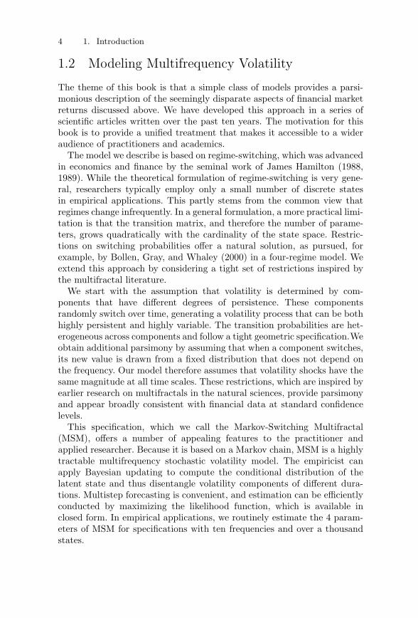
The theme of this book is that a simple class of models provides a parsi-monious description of the seemingly disparate aspects of financial marketreturns discussed above. We have developed this approach in a series ofscientific articles written over the past ten years. The motivation for thisbook is to provide a unified treatment that makes it accessible to a wideraudience of practitioners and academics.

The model we describe is based on regime-switching, which was advancedin economics and finance by the seminal work of James Hamilton (1988,1989). While the theoretical formulation of regime-switching is very gene-ral, researchers typically employ only a small number of discrete statesin empirical applications. This partly stems from the common view thatregimes change infrequently. In a general formulation, a more practical limi-tation is that the transition matrix, and therefore the number of parame-ters, grows quadratically with the cardinality of the state space. Restric-tions on switching probabilities offer a natural solution, as pursued, forexample, by Bollen, Gray, and Whaley (2000) in a four-regime model. Weextend this approach by considering a tight set of restrictions inspired bythe multifractal literature.

We start with the assumption that volatility is determined by com-ponents that have different degrees of persistence. These componentsrandomly switch over time, generating a volatility process that can be bothhighly persistent and highly variable. The transition probabilities are het-erogeneous across components and follow a tight geometric specification.Weobtain additional parsimony by assuming that when a component switches,its new value is drawn from a fixed distribution that does not depend onthe frequency. Our model therefore assumes that volatility shocks have thesame magnitude at all time scales. These restrictions, which are inspired byearlier research on multifractals in the natural sciences, provide parsimonyand appear broadly consistent with financial data at standard confidencelevels.

This specification, which we call the Markov-Switching Multifractal(MSM), offers a number of appealing features to the practitioner andapplied researcher. Because it is based on a Markov chain, MSM is a highlytractable multifrequency stochastic volatility model. The empiricist canapply Bayesian updating to compute the conditional distribution of thelatent state and thus disentangle volatility components of different dura-tions. Multistep forecasting is convenient, and estimation can be efficientlyconducted by maximizing the likelihood function, which is available inclosed form. In empirical applications, we routinely estimate the 4 param-eters of MSM for specifications with ten frequencies and over a thousandstates.

1.2 Modeling Multifrequency Volatility 5

Our research shows that MSM can outperform some of the most reli-able forecasting models currently in use, including Generalized ARCH(“GARCH,” Bollerslev, 1986) and related models, both in- and out-of-sample. These improvements are especially pronounced in the medium andlong run, and have been confirmed and extended in a variety of financialseries (e.g., Bacry, Kozhemyak, and Muzy, 2008; Lux, 2008). MSM alsocaptures well the power variation or “moment-scaling” of returns, worksequally well in discrete time and in continuous time, and generalizes tomultivariate settings.

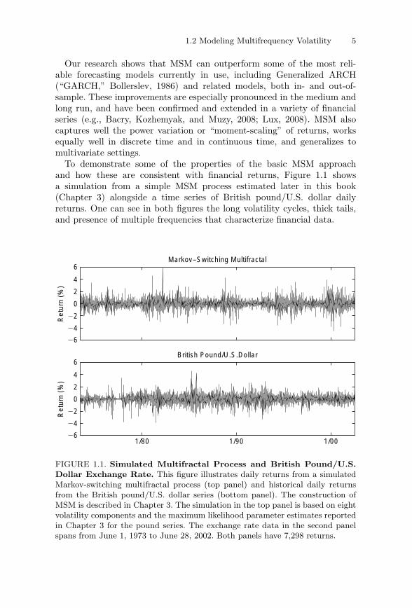
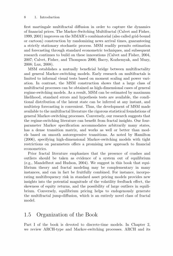
To demonstrate some of the properties of the basic MSM approachand how these are consistent with financial returns, Figure 1.1 showsa simulation from a simple MSM process estimated later in this book(Chapter 3) alongside a time series of British pound/U.S. dollar dailyreturns. One can see in both figures the long volatility cycles, thick tails,and presence of multiple frequencies that characterize financial data.

26

24

22

0

2

4

6

1/80 1/90 1/00

British Pound/U.S.Dollar

Ret

urn

(%)

Ret

urn

(%)

26

24

22

0

2

4

6Markov–Switching Multifractal

FIGURE 1.1. Simulated Multifractal Process and British Pound/U.S.Dollar Exchange Rate. This figure illustrates daily returns from a simulatedMarkov-switching multifractal process (top panel) and historical daily returnsfrom the British pound/U.S. dollar series (bottom panel). The construction ofMSM is described in Chapter 3. The simulation in the top panel is based on eightvolatility components and the maximum likelihood parameter estimates reportedin Chapter 3 for the pound series. The exchange rate data in the second panelspans from June 1, 1973 to June 28, 2002. Both panels have 7,298 returns.

6 1. Introduction

1.3 Pricing Multifrequency Risk

We explore the pricing implications of multifrequency risk by embed-ding MSM within an economic equilibrium framework. We assume thatfundamentals, such as dividend news, are subject to multifrequency volatil-ity risk, and we value the resulting cash flow stream in a standardconsumption-based model, as developed in Lucas (1978) and surveyedin Campbell (2003). The assumption that fundamentals are exposed tomultifrequency risk seems reasonable given the heterogeneity of the newsthat drive financial returns, and the pervasive evidence of multifractalityin weather patterns and other natural phenomena affecting the economy.Because MSM has a Markov structure, the resulting equilibrium is tractableand can be estimated by maximizing the likelihood of the excess returnseries, which is again available in closed form.

The MSM equilibrium model can capture the extreme realizations ofactual equity returns. In examples calibrated to U.S. aggregate equity, smallbut persistent changes in dividend news volatility generate substantial pricemovements, which are comparable in size to the most extreme histori-cal returns. Multifrequency risk also helps to explain the large differencebetween dividend and stock volatility that has long presented a puzzle toresearchers (Shiller, 1981). For instance, in a classic paper John Campbelland Ludger Hentschel (1992) use a quadratic GARCH specification to fitdividend news, and show that the variance of returns exceeds the varianceof dividends by about 1 to 2%. They attribute this modest amplification tothe property of GARCH-type specifications that the volatility of volatilitycan only be large if volatility itself is large. In our multifrequency environ-ment, the variance of returns exceeds the variance of dividends by about20 to 40%, which brings us substantially closer to the amplification levelsobserved in practice.

Multifrequency risk is easily incorporated into the drift of fundamen-tals, such as aggregate consumption and dividend news. As in the work ofRavi Bansal and Amir Yaron (2004), we can use a reasonable level of riskaversion to match the equity premium and still generate a substantialcontribution of equilibrium feedback to dividend volatility. The exten-sion also offers a pure regime-switching formulation of long-run risks ina multifrequency environment.

In order to match the skewness of equity returns, we consider economiesin which the volatility state is not directly observable by market partici-pants. We derive the novel theoretical result that investors should learnabruptly about volatility increases (bad news) but slowly about volatilitydecreases (good news). Learning about a volatility increase should beabrupt because outliers are highly improbable if in fact volatility remainslow. By contrast, realizations near the mean are a likely outcome under

1.4 Contributions to Multifractal Literature 7

any volatility scenario, and hence investors should learn slowly about avolatility decrease. This learning asymmetry is a powerful source of negativeskewness in returns.

Our learning results complement earlier research by Pietro Veronesi onhow information quality affects stock returns. Whereas Veronesi (2000)considers learning about the latent drift in a two-state Lucas economy, ourinvestors receive signals about an arbitrary number of dividend volatilitycomponents. By incorporating multiple shocks of heterogeneous durations,we obtain a structural learning model that can be applied to higher-frequency stock returns, in contrast to the lower-frequency calibrationstypically considered in the learning literature. More broadly, multifre-quency equilibrium modeling can be viewed as a first step toward bringingtogether the lower-frequency macro-finance and higher-frequency financialeconometrics literatures.

Examining the equilibrium implications of multifrequency risk in con-tinuous time provides additional insights. We consider an economy inwhich consumption and dividends follow continuous Ito diffusions. Markovswitches in the drift or volatility of fundamentals induce endogenous jumpsin equilibrium prices, in contrast to the exogenous price discontinuities typ-ically postulated in the literature. The multifrequency specification furthergenerates many small jumps, a few moderate jumps, and rare large jumps,while also producing additional features such as correlation between jumpsin volatility and prices. Previous literature also emphasizes the empiricalappeal of these properties, but generally assumes that they are exogenousfeatures of the price process (e.g., Bakshi, Cao, and Chen, 1997; Bates,2000; Duffie, Pan, and Singleton, 2000; Eraker, 2004; Eraker, Johannes,and Polson, 2003; Madan, Carr, and Chang, 1998). In our equilibrium,when the number of volatility components goes to infinity, the stock priceweakly converges to the sum of a continuous multifractal diffusion and aninfinite intensity pure jump process, producing a new stochastic processthat we call a multifractal jump-diffusion.

1.4 Contributions to Multifractal Literature

The research described in this book makes several contributions to theextensive literature on fractals and multifractals. Earlier work in thenatural sciences had focused on developing multifractal measures to rep-resent the distribution of physical quantities, such as the distribution ofminerals in the Earth’s crust or the distribution of energy in turbulentdissipation. New frontiers of research were opened by the developmentof multifractal diffusions. Specifically, the Multifractal Model of AssetReturns (“MMAR,” Calvet, Fisher, and Mandelbrot, 1997) proposed the

8 1. Introduction

first martingale multifractal diffusion in order to capture the dynamicsof financial prices. The Markov-Switching Multifractal (Calvet and Fisher,1999, 2001) improves on the MMAR’s combinatorial (also called grid-boundor cartoon) construction by randomizing news arrival times, guaranteeinga strictly stationary stochastic process. MSM readily permits estimationand forecasting through standard econometric techniques, and subsequentresearch continues to build on these innovations (Calvet and Fisher, 2004,2007; Calvet, Fisher, and Thompson 2006; Bacry, Kozhemyak, and Muzy,2008; Lux, 2008).

MSM establishes a mutually beneficial bridge between multifractalityand general Markov-switching models. Early research on multifractals islimited to informal visual tests based on moment scaling and power vari-ation. In contrast, the MSM construction shows that a large class ofmultifractal processes can be obtained as high-dimensional cases of generalregime-switching models. As a result, MSM can be estimated by maximumlikelihood, standard errors and hypothesis tests are available, the condi-tional distribution of the latent state can be inferred at any instant, andmultistep forecasting is convenient. Thus, the development of MSM madeavailable to the multifractal literature the rigorous statistical foundations ofgeneral Markov-switching processes. Conversely, our research suggests thatthe regime-switching literature can benefit from fractal insights. Our four-parameter Markov specification accommodates arbitrarily many states,has a dense transition matrix, and works as well or better than mod-els based on smooth autoregressive transitions. As noted by Hamilton(2006), specifying high-dimensional Markov-switching models with tightrestrictions on parameters offers a promising new approach to financialeconometrics.

Prior fractal literature emphasizes that the presence of crashes andoutliers should be taken as evidence of a system out of equilibrium(e.g., Mandelbrot and Hudson, 2004). We suggest in this book that equi-librium theory and fractal modeling may be complementary in manyinstances, and can in fact be fruitfully combined. For instance, incorpo-rating multifrequency risk in standard asset pricing models provides newinsights into the potential magnitude of the volatility feedback effect, theskewness of equity returns, and the possibility of large outliers in equili-brium. Conversely, equilibrium pricing helps to endogenously generatethe multifractal jump-diffusion, which is an entirely novel class of fractalmodel.

1.5 Organization of the Book

Part I of the book is devoted to discrete-time models. In Chapter 2,we review ARCH-type and Markov-switching processes. ARCH and its

1.5 Organization of the Book 9

numerous variants, which are now essential to financial market practitioners,are based on smooth linear variations in volatility and a single decay ratein basic formulations. Markov-switching models have become increasinglyuseful in financial econometrics and represent one of the foundations of ourapproach. Chapter 3 introduces the workhorse of the book, the Markov-Switching Multifractal (MSM), which permits a rich diversity of volatilityshocks. MSM produces good volatility forecasts, especially at longer hori-zons, and outperforms standard processes in- and out-of-sample. Chapter 4establishes that the approach easily generalizes to several assets. In an empir-ical application, multivariate MSM provides reasonable estimates of thevalue-at-risk inherent in a single currency or a portfolio of currencies.

Part II shows that multifrequency modeling works equally well in contin-uous time. Chapter 5 provides background material on self-similar processesand multifractal measures. Self-similar processes, such as Brownian motionand Levy stable processes, assume that the unconditional distribution ofreturns is identical across all time horizons, and do not adequately controlfor time-varying volatility. These models do, however, foreshadow certainaspects of the multifrequency approach that we develop in subsequent chap-ters. Multifractal measures were first applied in the natural sciences, andprovide another building block of the MSM approach. Chapter 6 presentsthe earliest multifractal diffusion, the MMAR, defined as a Brownianmotion in trading time, where trading time is the cumulative distributionfunction of a multifractal measure obtained by recursively reallocating masswithin a finite time interval.

Chapter 7 shows that the discrete-time MSM approach developed inChapter 3 easily extends to continuous time and solves the nonstationar-ity problems inherent in the MMAR. We demonstrate weak convergenceof the discrete-time construction to the continuous-time process, and theconnection between the parameters is available in closed form. The limitMSM process contains an infinite number of frequencies and its samplepaths are characterized by a continuum of local scales. Chapter 8 presentsempirical evidence on the power variation of returns at various frequenciesand demonstrates its consistency with the multifractal model.

Part III of the book derives equilibrium implications of multifrequencyvolatility. In the discrete-time approach of Chapter 9, we assume that thevolatility of dividend news follows an MSM process and we derive theendogenous stock return process. We find that variations in multifrequencyvolatility shocks can have substantial feedback effects on overall financialvolatility. We also show that learning about volatility is a powerful sourceof endogenous skewness in returns, and develop a multifrequency versionof long-run risk. Chapter 10 considers equilibrium stock returns in contin-uous time, focusing on endogenous jump-diffusions and convergence to amultifractal jump-diffusion. Unless stated otherwise, all proofs are in theAppendix.

10 1. Introduction

The book should be accessible to practitioners working on risk manage-ment and volatility forecasting applications. It is also suited for researchersin economics, finance, econometrics, and statistics, or natural scientistsand general readers interested in fractal modeling. Graduate students ineconomics and finance, as well as advanced undergraduates with solid foun-dations in econometrics, may find useful ideas and inspiration for futureresearch.

2Background: Discrete-Time VolatilityModeling

In this chapter, we briefly discuss several common approaches to modelingfinancial volatility, including GARCH, stochastic volatility, and Markov-switching formulations. Our goal is not to provide a complete survey, but tobriefly introduce key models that facilitate the development of MSM and pro-vide comparisons. Excellent surveys of the literature can be found in Boller-slev, Engle, and Nelson (1994), Engle (2004), Ghysels, Harvey, and Renault(1996), Hamilton (2006), Hamilton and Raj (2002), and Shephard (2005).

2.1 Autoregressive Volatility Modeling

The most common approach to volatility modeling builds on the general-ized autoregressive conditional heteroskedasticity (GARCH) class (Engle,1982; Bollerslev, 1986), in which volatility follows a smooth autoregressivetransition. Let rt denote the log return of a financial asset, such as anexchange rate, between dates t − 1 and t. Under GARCH(p, q), the returnis specified as

rt = h1/2t εt,

where ht denotes the conditional variance of rt at date t − 1, and εt

is an independently and identically distributed (i.i.d.) random variablewith zero mean and unit variance. The conditional variance ht follows theautoregressive process:

ht = ω +p∑

i=1

βiht−i +q∑

j=1

αjr2t−j ,

and is therefore a smooth deterministic function of past squared returns.The noise εt can be a standard normal (Engle, 1982; Bollerslev, 1986).In order to better capture the outliers of financial series, researchers haveconsidered numerous extensions where εt has a distribution with thicker

14 2. Background: Discrete-Time Volatility Modeling

tails than the Gaussian, such as the Student-t (Bollerslev, 1987), the gen-eralized error distribution (Nelson, 1991), or nonparametric specifications(Engle and Gonzalez-Rivera, 1991).1

The GARCH conditional variance ht is known to the econometricianat date t − 1, and the conditional distribution of the period-t return, rt =h

1/2t εt, is a rescaled version of the noise εt. When the specification for εt has

a closed-form density, the conditional distribution of rt and more generallythe likelihood of the return series r1, . . . , rT are available in closed form,which facilitates maximum likelihood estimation.

Because GARCH variance follows a smooth autoregressive transition,standard specifications have difficulty capturing the sudden changes involatility exhibited by many financial series. For this reason, econometri-cians have considered extensions, called stochastic volatility models,2 inwhich volatility is hit by separate shocks:

ln(ht) = ω +p∑

i=1

βi ln(ht−i) +q∑

j=1

αjr2t−j + ηt.

The noise ηt is realized at date t jointly with the return rt. If the econometri-cian has access only to returns, the volatility state is not directly observableand must be imputed. Consequently, the density of rt = h

1/2t εt is unavail-

able in closed form and estimation proceeds by moment-based inference orsimulation. As will be discussed in Chapter 3, the multifrequency approachalso incorporates volatility-specific shocks. In contrast to standard stochas-tic volatility models, however, our model generates a closed-form likelihood,which permits convenient and efficient likelihood-based estimation.

1Extensions and applications ofGARCH infinance and economics have been the objectof a vast literature, which includes, among many other contributions, Baillie and Bollerslev(1989), Barone-Adesi, Engle, and Mancini (2008), Bera and Lee (1992), Bollerslev, Chou,and Kroner (1992), Bollerslev, Engle, and Nelson (1994), Campbell and Hentschel (1992),Chou, Engle, and Kane (1992), Diebold (1988), Drost and Nijman (1993), Engle (2002a,2004), Engle and Rangel (2008), Engle and Ng (1993), Engle, Lilien, and Robins (1987),French, Schwert, and Stambaugh (1987), Gallant and Tauchen (1989), Gallant, Hsieh,and Tauchen (1991), Gallant, Rossi, and Tauchen (1992, 1993), Geweke (1989), Glosten,Jagannathan, and Runkle (1993), Gourieroux and Montfort (1992), Nelson (1989, 1990,1991), Nijman and Palm (1993), Pagan and Hong (1991), Pagan and Schwert (1990), Rossi(1996), Schwert (1989), Sentana (1995), and Zakoian (1994).

2Contributions to the stochastic volatility literature include Andersen (1994, 1996),Andersen and Sørensen (1996), Andersen, Benzoni, and Lund (2002), Bakshi, Cao, andChen (1997), Barndorff-Nielsen and Shephard (2001, 2003), Bates (1996), Chernov,Gallant, Ghysels, and Tauchen (2003), Clark (1973), Eraker (2001), Eraker, Johannesand Polson (2003), Gallant, Hsieh, and Tauchen (1997), Ghysels, Harvey, and Renault(1996), Harvey, Ruiz, and Shephard (1994), Heston (1993), Hull and White (1987),Jacquier, Polson, and Rossi (1994, 2004), Johannes, Polson, and Stroud (2002), Jones(2003), Kim, Shephard, and Chib (1998), Melino and Turnbull (1990), Renault andTouzi (1996), Rosenberg (1972), Shephard (2005), Stein and Stein (1991), Taylor (1982,1986), and Wiggins (1987).

2.1 Autoregressive Volatility Modeling 15

Standard GARCH models provide good forecasts of short-run volatil-ity dynamics, but often have difficulties capturing lower-frequency cycles.Consider, for instance, GARCH(1, 1), which is one of the best perform-ing models in the GARCH literature (e.g., Akgiray, 1989; Andersen andBollerslev, 1998a; Hansen and Lunde, 2005; Pagan and Schwert, 1990; Westand Cho, 1995). Volatility follows

ht = ω + βht−1 + αr2t−1,

and forward iteration implies

ht = ω + αr2t−1 + β(ω + αr2

t−2 + βht−2)

=ω

1 − β+ α

∞∑

i=1

βi−1r2t−i.

A volatility shock declines at a single exponential rate β. In practice, thisimplies that GARCH(1, 1) picks up the short-run autocorrelation in volatil-ity but cannot easily capture longer cycles. More generally, stationarityplaces practical limits on the type of lower-frequency cycles that can becaptured by a GARCH(p, q) model.

For this reason, econometricians have considered volatility models thatincorporate stronger persistence in squared returns. Specifically, while typ-ical ARCH/GARCH processes have weak persistence, long memory insquared returns is a characteristic feature of fractionally integrated GARCH(Baillie, Bollerslev, and Mikkelsen, 1996)3 and long-memory stochasticvolatility (Breidt, Crato, and de Lima, 1998; Comte and Renault, 1998;Harvey, 1998; Robinson and Zaffaroni, 1998).4 Long-memory processes cap-ture very low-frequency cycles in financial or other data by permittingslowly declining autocorrelations of a hyperbolic form at long horizons. Bycontrast, short-memory processes are characterized by the fast exponentialdeclines of autocorrelations. Long memory was first analyzed in the con-text of fractional integration of Brownian motion by Mandelbrot (1965a)and Mandelbrot and van Ness (1968).5 It has been documented in squaredand absolute returns for many financial data sets (Dacorogna et al., 1993;Ding, Granger, and Engle, 1993; Taylor, 1986). We refer the reader toBaillie (1996), Beran (1994), and Robinson (2003) for excellent surveys oflong memory in econometrics and statistics.

3Ding and Granger (1996) develop the related Long Memory ARCH process.4Additional contributions include Deo and Hurvich (2001), Deo, Hurvich, and Lu

(2006), Goncalves da Silva and Robinson (2007), Hurvich, Moulines, and Soulier (2005),Hurvich and Ray (2003), Robinson (2001), and Zaffaroni (2007).

5Granger and Joyeux (1980) and Hosking (1981) advanced the use of long memoryin economics by introducing a discrete-time counterpartof fractional Brownian motion,the autoregressive fractionally integrated moving average (ARFIMA) process.

16 2. Background: Discrete-Time Volatility Modeling

Another important strand of the ARCH literature attempts to jointlycapture volatility dynamics in several financial markets. MultivariateGARCH, pioneered by Kraft and Engle (1982) and Bollerslev, Engle, andWooldridge (1988), is perhaps the most commonly used class of models,and has been extended in many directions.6 In Chapter 4 we show how tomodel multifrequency shocks in a multi-asset environment.

2.2 Markov-Switching Models

In contrast to the GARCH volatility models discussed earlier, stochasticregime-switching models permit the conditional mean and variance of finan-cial returns to depend on an unobserved latent “state” that may changeunpredictably. The application of regime-switching models in economics andfinance was pioneered by Hamilton (1988, 1989, 1990), and a rich literaturehas emerged.7

The general approach considers a latent state Mt ∈{m1, ..., md

}, where

the positive integer d describes the number of possible states. Returns aregiven by

rt = μ(Mt) + σ(Mt) εt,

where μ(Mt) and σ(Mt) are, respectively, the state-dependent conditionalmean and variance of returns. The dynamics of the Markov chain Mt

are fully characterized by the transition matrix A = (ai,j)1≤i,j≤d withcomponents aij = P(Mt+1 = mj |Mt = mi).

Estimation and forecasting methods for regime-switching models are nowstandard. We provide details specific to our setting in the individual chap-ters, and the interested reader may refer to Hamilton (1994, Chapter 22)for further discussion of the general approach.

6Examples include Bollerslev (1990), Diebold and Nerlove (1989), Engle (1987,2002b), Engle and Kroner (1995), Engle and Mezrich (1996), Engle, Ng, and Rothschild(1990), Kraft and Engle (1982), and Ledoit, Santa-Clara, and Wolf (2003).

7The likelihood-based estimation of Markov-switching processes was developed byLindgren (1978) and Baum et al. (1980) in the statistics literature. Hamilton (1988, 1989,1990) introduced these processes to the economics literature and spurred the developmentof a large body of research. Contributions to the original version of the model advanceestimation and testing (Albert and Chib, 1993; Garcia, 1998; Hansen, 1992; Shephard,1994), and investigate a wide range of empirical applications (e.g., Hamilton, 1988; Garciaand Perron, 1996). The approach has been extended to incorporate GARCH transitions(Cai, 1994; Gray, 1996; Hamilton and Susmel, 1994; Kim, 1994; Kim and Nelson, 1999;Klaassen, 2002), vector processes (Hamilton and Lin, 1996; Hamilton and Perez-Quiros,1996), and time-varying transition probabilities (Diebold, Lee, and Weinbach, 1994;Durland and McCurdy, 1994; Filardo, 1994; Maheu and McCurdy, 2000; Perez-Quirosand Timmermann, 2000). See Hamilton and Raj (2002) and Hamilton (2006) for a survey.

2.2 Markov-Switching Models 17

In typical applications, researchers use Markov switching to modellow-frequency variations and rely on other techniques for shorter-rundynamics. For example, Markov-switching ARCH and GARCH processesseparately specify regime shifts at low frequencies, smooth autoregressivevolatility transitions at midrange frequencies, and a thick-tailed condi-tional distribution of returns at high-frequency (Cai, 1994; Hamilton andSusmel, 1994; Gray, 1996; Klaassen, 2002). In Chapter 3, we develop theMarkov-Switching Multifractal approach based on pure regime-switching atall frequencies, and we compare this model with earlier Markov-switchingformulations.

3The Markov-Switching Multifractal(MSM) in Discrete Time

In this chapter, we present the discrete-time version of the main modelin this book, the Markov-Switching Multifractal (MSM). MSM closelymatches the intuition that a range of economic uncertainties with vary-ing degrees of persistence impact financial markets. Using a tight setof restrictions inspired by the multifractal literature, we define a pureregime-switching specification with multiple frequencies, arbitrarily manystates, and a dense transition matrix. The MSM construction is strikinglyparsimonious as it requires only four parameters.

MSM volatility is derived by multiplying together a finite number ofrandom first-order Markov components. We assume for parsimony that thevolatility components are identical except for differences in their switch-ing probabilities, which follow an approximately geometric progression.The construction delivers a multifrequency stochastic volatility model witha closed-form likelihood, enabling us for the first time to apply a stan-dard econometric toolkit to estimating and forecasting using a multifractalmodel.

An empirical investigation of four daily currency series shows that MSMperforms well in comparison with leading forecasting models, includingGARCH(1,1), both in- and out-of-sample. In the data, MSM has a higherlikelihood than GARCH for all currencies, and the improvement is statisti-cally significant. Since both models have the same number of parameters, themultifractal is also preferred by standard selection criteria. Out-of-sample,MSM matches the accuracy of GARCH forecasts at very short horizonssuch as one day, and provides substantially better forecasts at longer hori-zons, such as 20 to 50 business days. We also demonstrate that the multi-fractal model improves on Markov-switching GARCH (MS-GARCH) andfractionally integrated GARCH (FIGARCH) out of sample.

Traditional Markov-switching approaches such as MS-GARCH useregime-switching only for low-frequency events, while also using linearautoregressive transitions at medium frequencies and a thick-tailed con-ditional distribution of returns. By contrast, MSM captures long-memoryfeatures, intermediate frequency volatility dynamics, and thick tails inreturns all with a single regime-switching approach. It is noteworthy that

This chapter is based on an earlier paper: “How to Forecast Long-Run Volatility: Regime-Switching and the Estimation of Multifractal Processes” (with A. Fisher), Econometrics,2: 49–83, Spring 2004.

20 3. The Markov-Switching Multifractal (MSM) in Discrete Time

a single mechanism can play all three of these roles so effectively, and theinnovation that achieves this surprising economy of modeling technique isbased on scale-invariance.

3.1 The MSM Model of Stochastic Volatility

3.1.1 DefinitionWe consider a financial series Pt defined in discrete time on the regular gridt = 0, 1, 2, . . . ,∞. In applications, Pt will be the price of a financial asset orexchange rate. Let rt ≡ ln(Pt/Pt−1) denote the log-return. The economy isdriven by a first-order Markov state vector with k components:

Mt =(M1,t;M2,t; . . . ;Mk,t

)∈ R

k+.

The components of Mt have the same marginal distribution but evolve atdifferent frequencies, as we now explain.

Assume that the volatility state vector has been constructed up to datet−1. For each k∈{1, . . . , k}, the next period multiplier Mk,t is drawn froma fixed distribution M with probability γk, and is otherwise equal to itsprevious value: Mk,t =Mk,t−1. The dynamics of Mk,t can be summarized as

Mk,t drawn from distribution M with probability γk

Mk,t = Mk,t−1 with probability 1 − γk,

where the switching events and new draws from M are assumed to beindependent across k and t. We require that the distribution of M has apositive support and unit mean: M ≥ 0 and E(M) = 1.

Under these assumptions, the random multipliers Mk,t are persistent andnonnegative, and satisfy E(Mk,t) = 1. The multipliers differ in their transi-tion probabilities γk but not in their marginal distribution M . Componentsof different frequencies are mutually independent; that is, the variablesMk,t and Mk′,t′ are independent if k differs from k′. These features greatlycontribute to the parsimony of the model.

We model stochastic volatility by

σ(Mt) ≡ σ

⎛

⎝k∏

i=1

Mk,t

⎞

⎠1/2

,

where σ is a positive constant. Returns rt are then

rt = σ(Mt)εt, (3.1)

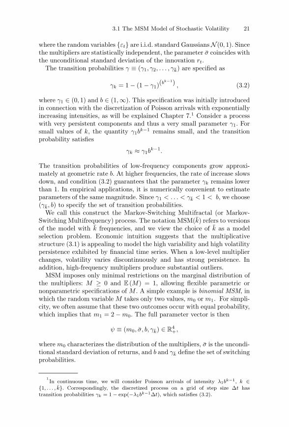
3.1 The MSM Model of Stochastic Volatility 21

where the random variables {εt} are i.i.d. standard Gaussians N (0, 1). Sincethe multipliers are statistically independent, the parameter σ coincides withthe unconditional standard deviation of the innovation rt.

The transition probabilities γ ≡ (γ1, γ2, . . . , γk) are specified as

γk = 1 − (1 − γ1)(bk−1) , (3.2)

where γ1 ∈ (0, 1) and b ∈ (1,∞). This specification was initially introducedin connection with the discretization of Poisson arrivals with exponentiallyincreasing intensities, as will be explained Chapter 7.1 Consider a processwith very persistent components and thus a very small parameter γ1. Forsmall values of k, the quantity γ1b

k−1 remains small, and the transitionprobability satisfies

γk ≈ γ1bk−1.

The transition probabilities of low-frequency components grow approxi-mately at geometric rate b. At higher frequencies, the rate of increase slowsdown, and condition (3.2) guarantees that the parameter γk remains lowerthan 1. In empirical applications, it is numerically convenient to estimateparameters of the same magnitude. Since γ1 < . . . < γk < 1 < b, we choose(γk, b) to specify the set of transition probabilities.

We call this construct the Markov-Switching Multifractal (or Markov-Switching Multifrequency) process. The notation MSM(k) refers to versionsof the model with k frequencies, and we view the choice of k as a modelselection problem. Economic intuition suggests that the multiplicativestructure (3.1) is appealing to model the high variability and high volatilitypersistence exhibited by financial time series. When a low-level multiplierchanges, volatility varies discontinuously and has strong persistence. Inaddition, high-frequency multipliers produce substantial outliers.

MSM imposes only minimal restrictions on the marginal distribution ofthe multipliers: M ≥ 0 and E (M) = 1, allowing flexible parametric ornonparametric specifications of M . A simple example is binomial MSM, inwhich the random variable M takes only two values, m0 or m1. For simpli-city, we often assume that these two outcomes occur with equal probability,which implies that m1 = 2 − m0. The full parameter vector is then

ψ ≡ (m0, σ, b, γk) ∈ R4+,

where m0 characterizes the distribution of the multipliers, σ is the uncondi-tional standard deviation of returns, and b and γk define the set of switchingprobabilities.

1In continuous time, we will consider Poisson arrivals of intensity λ1bk−1, k ∈

{1, . . . , k}. Correspondingly, the discretized process on a grid of step size Δt hastransition probabilities γk = 1 − exp(−λ1bk−1Δt), which satisfies (3.2).

22 3. The Markov-Switching Multifractal (MSM) in Discrete Time

We can naturally consider other parametric specifications for the dis-tribution M . For example, multinomial MSM extends binomial MSM byallowing any discrete distribution satisfying the positivity and unit meanrequirements. Continuous densities can also be useful. In Chapters 7 and 8we assume that the distribution of M is lognormal, which defines lognor-mal MSM. In the remainder of Chapter 3 and in Chapter 4, we will seethat even the simplest version of binomial MSM with equal probabilities issufficient to produce good results in- and out-of-sample.

3.1.2 Basic PropertiesMSM(k) permits the parsimonious specification of a high-dimensional statespace. Assume, for instance, that the distribution M is a binomial. Eachvolatility component Mk,t is either high or low, and the state vector Mt cantake 2k possible values. We will routinely work with models that have 10components, or 210 = 1,024 states. MSM is also remarkably parsimonious.In a general Markov chain, the size of the transition matrix is equal tothe square of the number of states. For instance, a Markov chain with 210

states generally needs to be parametrized by 210×210 or more than a millionelements. In contrast, binomial MSM only requires four parameters.

Because binomial MSM is a pure regime-switching model, we can use allthe tools that commonly apply to this class of processes. In the next sec-tion, we will review Bayesian updating and write the closed-form likelihoodfunction. This book therefore brings to the literature a class of stochas-tic volatility models that have multiple degrees of persistence and canbe estimated by maximum likelihood. The approach also creates a bridgebetween Markov-switching and multifractals, and permits the applicationof standard inference techniques to multifractal processes. The connectionbetween fractal modeling and MSM will become more apparent in Part II.

A representative return series is illustrated in Figure 3.1. The graphreveals large heterogeneity in volatility levels and substantial outliers. Thisis notable since the return process has by construction finite moments ofevery order. It would be easy to obtain thick tails by considering i.i.d. shocksεt with Paretian distributions. In this chapter, however, we focus on theGaussian case for several reasons. First, the likelihood is then availablein closed form. Second, we will show that even when εt is Gaussian, high-frequency regime switches are sufficient to mimic in finite samples the heavytails exhibited by financial data. Finally, the basic specification performswell relative to existing competitors and provides a useful benchmark forfuture refinements.

3.1.3 Low-Frequency Components and Long MemoryThe MSM construction permits low-frequency regime shifts and longvolatility cycles in sample paths. We will see that in exchange rate series,

3.1 The MSM Model of Stochastic Volatility 23

0 1000 2000 3000 4000 5000 6000 700025

22

0

2

5R

etur

n (%

)

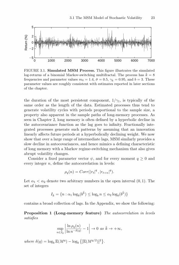
FIGURE 3.1. Simulated MSM Process. This figure illustrates the simulatedlog-returns of a binomial Markov-switching multifractal. The process has k = 8frequencies and parameter values m0 = 1.4, σ = 0.5, γk = 0.95, and b = 3. Theseparameter values are roughly consistent with estimates reported in later sectionsof the chapter.

the duration of the most persistent component, 1/γ1, is typically of thesame order as the length of the data. Estimated processes thus tend togenerate volatility cycles with periods proportional to the sample size, aproperty also apparent in the sample paths of long-memory processes. Asseen in Chapter 2, long memory is often defined by a hyperbolic decline inthe autocovariance function as the lag goes to infinity. Fractionally inte-grated processes generate such patterns by assuming that an innovationlinearly affects future periods at a hyperbolically declining weight. We nowshow that over a large range of intermediate lags, MSM similarly provides aslow decline in autocovariances, and hence mimics a defining characteristicof long memory with a Markov regime-switching mechanism that also givesabrupt volatility changes.

Consider a fixed parameter vector ψ, and for every moment q ≥ 0 andevery integer n, define the autocorrelation in levels:

ρq(n) = Corr(|rt|q , |rt+n|q).

Let α1 < α2 denote two arbitrary numbers in the open interval (0, 1). Theset of integers

Ik = {n : α1 logb(bk) ≤ logb n ≤ α2 logb(b

k)}

contains a broad collection of lags. In the Appendix, we show the following:

Proposition 1 (Long-memory feature) The autocorrelation in levelssatisfies

supn∈Ik

∣∣∣∣ln ρq(n)lnn−δ(q) − 1

∣∣∣∣ → 0 as k → +∞,

where δ(q) = logb E(Mq) − logb

{[E(Mq/2)]2

}.

24 3. The Markov-Switching Multifractal (MSM) in Discrete Time

Multifrequency volatility is therefore consistent over a large range of lagswith the hyperbolic autocorrelation exhibited by many financial series.2

The proof of this result builds on the decomposition of log autocorrela-tion:

ln ρq(n) ≈k∑

k=1

lnE(Mq/2

k,t Mq/2k,t+n)

E(Mq),

and the mean-reversion property:

E(Mq/2k,t M

q/2k,t+n) = E(Mq)(1 − γk)n + [E(Mq/2)]2[1 − (1 − γk)n].

We infer:

ln ρq(n) ≈k∑

k=1

ln1 + (bδ(q) − 1)(1 − γ∗)nbk−k

bδ(q) , (3.3)

where the transition probability γ∗ = γk is a fixed parameter. For any n ∈Ik, consider k(n) such that nbk(n)−k ≈ 1, or equivalently k(n) ≈ k−logb(n).The kth addend in (3.3) is negligible if k < k(n), and close to −δ(q) ln b ifk > k(n), implying

ln ρq(n) ≈ −δ(q)[k − k(n)] ln b,

or ln [ρq(n)] ≈ −δ(q) ln n. We also note that for n sufficiently large, theautocorrelation transitions smoothly from a hyperbolic to an exponentialrate of decline.

The proof of Proposition 1 is reminiscent of Granger (1980) and Robinson(1978), who generate long memory by aggregating first-order autoregressiveprocesses with heterogeneous coefficients.3 MSM components are similarlymean-reverting with diverse decay rates, and their product correspondinglyexhibits hyperbolic decay. The result also complements earlier researchthat has emphasized the difficulty of distinguishing between long mem-ory and structural change in finite samples (e.g., Bhattacharya, Gupta,and Waymire, 1983; Diebold and Inoue, 2001; Granger and Hyung, 1999;Hidalgo and Robinson, 1996; Klemes, 1974; Kunsch, 1986; Lobato andSavin, 1997). The structure provided by MSM permits direct analysis ofthe approximate shape of the autocorrelation function, and allows us toidentify the region of lags in which long memory-like behavior holds.

2See, for instance, Dacorogna et al. (1993), Ding, Granger, and Engle (1993), Baillie,

Bollerslev, and Mikkelsen (1996), and Gourieroux and Jasiak (2002).3Ding and Granger (1996) use similar aggregation insights to specify a model of

long-memory volatility.

3.2 Maximum Likelihood Estimation 25

MSM thus illustrates that a Markov chain can imitate one of the definingfeatures of long memory, a hyperbolic decline of the autocovariogram.4 Thecombination of long-memory behavior with sudden volatility movements inMSM has a natural appeal for financial econometrics.

3.2 Maximum Likelihood Estimation

When the multiplier M has a discrete distribution, there exist a finitenumber of volatility states. Standard filtering methods then provide thelikelihood function in closed form.

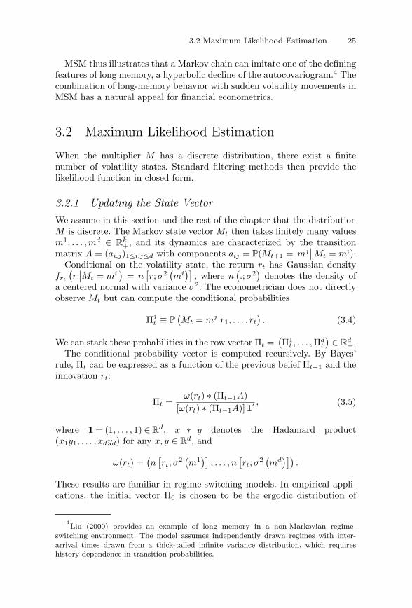
3.2.1 Updating the State VectorWe assume in this section and the rest of the chapter that the distributionM is discrete. The Markov state vector Mt then takes finitely many valuesm1, . . . , md ∈ R

k+, and its dynamics are characterized by the transition

matrix A = (ai,j)1≤i,j≤d with components aij = P(Mt+1 = mj∣∣ Mt = mi).

Conditional on the volatility state, the return rt has Gaussian densityfrt

(r∣∣Mt = mi

)= n

[r;σ2

(mi

)], where n

(.;σ2

)denotes the density of

a centered normal with variance σ2. The econometrician does not directlyobserve Mt but can compute the conditional probabilities

Πjt ≡ P

(Mt = mj |r1, . . . , rt

). (3.4)

We can stack these probabilities in the row vector Πt =(Π1

t , . . . ,Πdt

)∈ R

d+.

The conditional probability vector is computed recursively. By Bayes’rule, Πt can be expressed as a function of the previous belief Πt−1 and theinnovation rt:

Πt =ω(rt) ∗ (Πt−1A)

[ω(rt) ∗ (Πt−1A)]1′ , (3.5)

where 1 = (1, . . . , 1) ∈ Rd, x ∗ y denotes the Hadamard product

(x1y1, . . . , xdyd) for any x, y ∈ Rd, and

ω(rt) =(n

[rt;σ2 (

m1)] , . . . , n[rt;σ2 (

md)])

.

These results are familiar in regime-switching models. In empirical appli-cations, the initial vector Π0 is chosen to be the ergodic distribution of

4Liu (2000) provides an example of long memory in a non-Markovian regime-

switching environment. The model assumes independently drawn regimes with inter-arrival times drawn from a thick-tailed infinite variance distribution, which requireshistory dependence in transition probabilities.

26 3. The Markov-Switching Multifractal (MSM) in Discrete Time

the Markov process. Since the multipliers are mutually independent, theergodic distribution is given by Πj

0 =∏k

l=1 P(M = mjl ) for all j.

The multifrequency model can generate rich forecast dynamics. Considerthe vector of past and current returns

Rt = {r1, . . . , rt} .

For each k, the n-step component forecast E(Mk,t+n|Rt) monotonicallyreverts to E(M) = 1 as the time horizon n increases, but the volatility fore-casts E

(σ2 (Mt+n) |Rt

)need not be monotonic in n. Consider, for instance,

a state Mt with a low value of the transitory component Mk,t, and highvalues of M1,t, . . . , Mk−1,t. In such a state, current volatility σ2 (Mt) ishigh, but the volatility forecast E(σ2 (Mt+n) |Mt) can increase with n inthe short run before decreasing toward the long-run mean σ2 at longerhorizons. This suggests that MSM can provide finer filtering and forecaststhan a unifrequency model.

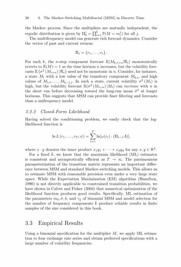
3.2.2 Closed-Form LikelihoodHaving solved the conditioning problem, we easily check that the log-likelihood function is

lnL (r1, . . . , rT ;ψ) =T∑

t=1

ln[ω(rt) · (Πt−1A)],

where x · y denotes the inner product x1y1 + · · · + xdyd for any x, y ∈ Rd.

For a fixed k, we know that the maximum likelihood (ML) estimatoris consistent and asymptotically efficient as T → ∞. The parsimoniousparameterization of the transition matrix represents an important differ-ence between MSM and standard Markov-switching models. This allows usto estimate MSM with reasonable precision even under a very large statespace. While the Expectation Maximization (EM) algorithm (Hamilton,1990) is not directly applicable to constrained transition probabilities, wehave shown in Calvet and Fisher (2004) that numerical optimization of thelikelihood function produces good results. Specifically, ML estimation ofthe parameters m0, σ, b, and γk of binomial MSM and model selection forthe number of frequency components k produce reliable results in finitesamples of the size considered in this book.

3.3 Empirical Results

Using a binomial specification for the multiplier M , we apply ML estima-tion to four exchange rate series and obtain preferred specifications with alarge number of volatility frequencies.

3.3 Empirical Results 27

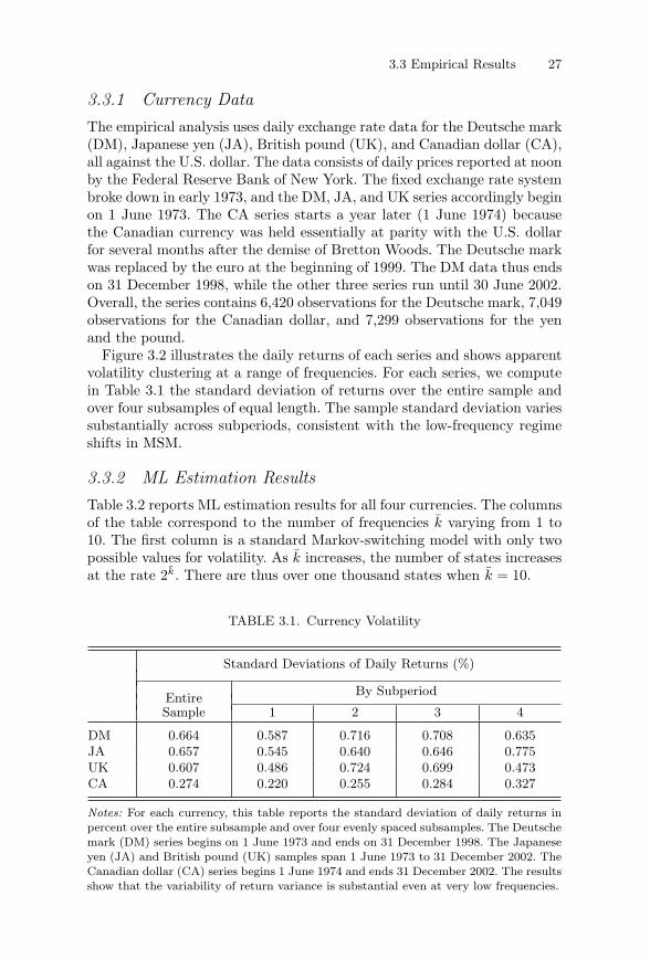
3.3.1 Currency DataThe empirical analysis uses daily exchange rate data for the Deutsche mark(DM), Japanese yen (JA), British pound (UK), and Canadian dollar (CA),all against the U.S. dollar. The data consists of daily prices reported at noonby the Federal Reserve Bank of New York. The fixed exchange rate systembroke down in early 1973, and the DM, JA, and UK series accordingly beginon 1 June 1973. The CA series starts a year later (1 June 1974) becausethe Canadian currency was held essentially at parity with the U.S. dollarfor several months after the demise of Bretton Woods. The Deutsche markwas replaced by the euro at the beginning of 1999. The DM data thus endson 31 December 1998, while the other three series run until 30 June 2002.Overall, the series contains 6,420 observations for the Deutsche mark, 7,049observations for the Canadian dollar, and 7,299 observations for the yenand the pound.

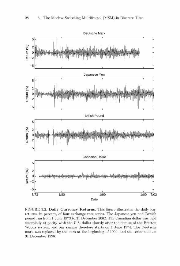
Figure 3.2 illustrates the daily returns of each series and shows apparentvolatility clustering at a range of frequencies. For each series, we computein Table 3.1 the standard deviation of returns over the entire sample andover four subsamples of equal length. The sample standard deviation variessubstantially across subperiods, consistent with the low-frequency regimeshifts in MSM.

3.3.2 ML Estimation ResultsTable 3.2 reports ML estimation results for all four currencies. The columnsof the table correspond to the number of frequencies k varying from 1 to10. The first column is a standard Markov-switching model with only twopossible values for volatility. As k increases, the number of states increasesat the rate 2k. There are thus over one thousand states when k = 10.

TABLE 3.1. Currency Volatility

Standard Deviations of Daily Returns (%)

By SubperiodEntireSample 1 2 3 4

DM 0.664 0.587 0.716 0.708 0.635JA 0.657 0.545 0.640 0.646 0.775UK 0.607 0.486 0.724 0.699 0.473CA 0.274 0.220 0.255 0.284 0.327

Notes: For each currency, this table reports the standard deviation of daily returns inpercent over the entire subsample and over four evenly spaced subsamples. The Deutschemark (DM) series begins on 1 June 1973 and ends on 31 December 1998. The Japaneseyen (JA) and British pound (UK) samples span 1 June 1973 to 31 December 2002. TheCanadian dollar (CA) series begins 1 June 1974 and ends 31 December 2002. The resultsshow that the variability of return variance is substantial even at very low frequencies.

28 3. The Markov-Switching Multifractal (MSM) in Discrete Time

25

22

0

2

5

British Pound

25

22

0

2

5

Japanese Yen

25

22

0

2

5

Deutsche Mark

6/73 1/80 1/90 1/00 7/02

25

22

0

2

5

Canadian Dollar

Ret

urn

(%)

Ret

urn

(%)

Ret

urn

(%)

Ret

urn

(%)

Date

FIGURE 3.2. Daily Currency Returns. This figure illustrates the daily log-returns, in percent, of four exchange rate series. The Japanese yen and Britishpound run from 1 June 1973 to 31 December 2002. The Canadian dollar was heldessentially at parity with the U.S. dollar shortly after the demise of the BrettonWoods system, and our sample therefore starts on 1 June 1974. The Deutschemark was replaced by the euro at the beginning of 1999, and the series ends on31 December 1998.

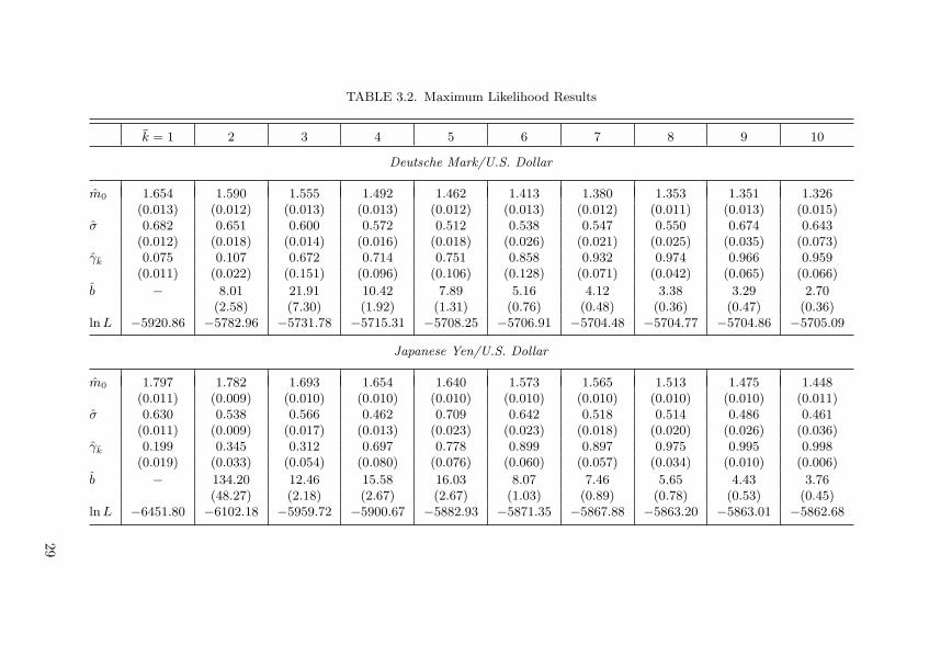
TABLE 3.2. Maximum Likelihood Results

k = 1 2 3 4 5 6 7 8 9 10

Deutsche Mark/U.S. Dollar

m0 1.654 1.590 1.555 1.492 1.462 1.413 1.380 1.353 1.351 1.326(0.013) (0.012) (0.013) (0.013) (0.012) (0.013) (0.012) (0.011) (0.013) (0.015)

σ 0.682 0.651 0.600 0.572 0.512 0.538 0.547 0.550 0.674 0.643(0.012) (0.018) (0.014) (0.016) (0.018) (0.026) (0.021) (0.025) (0.035) (0.073)

γk 0.075 0.107 0.672 0.714 0.751 0.858 0.932 0.974 0.966 0.959(0.011) (0.022) (0.151) (0.096) (0.106) (0.128) (0.071) (0.042) (0.065) (0.066)

b − 8.01 21.91 10.42 7.89 5.16 4.12 3.38 3.29 2.70(2.58) (7.30) (1.92) (1.31) (0.76) (0.48) (0.36) (0.47) (0.36)

ln L −5920.86 −5782.96 −5731.78 −5715.31 −5708.25 −5706.91 −5704.48 −5704.77 −5704.86 −5705.09

Japanese Yen/U.S. Dollar

m0 1.797 1.782 1.693 1.654 1.640 1.573 1.565 1.513 1.475 1.448(0.011) (0.009) (0.010) (0.010) (0.010) (0.010) (0.010) (0.010) (0.010) (0.011)

σ 0.630 0.538 0.566 0.462 0.709 0.642 0.518 0.514 0.486 0.461(0.011) (0.009) (0.017) (0.013) (0.023) (0.023) (0.018) (0.020) (0.026) (0.036)

γk 0.199 0.345 0.312 0.697 0.778 0.899 0.897 0.975 0.995 0.998(0.019) (0.033) (0.054) (0.080) (0.076) (0.060) (0.057) (0.034) (0.010) (0.006)

b − 134.20 12.46 15.58 16.03 8.07 7.46 5.65 4.43 3.76(48.27) (2.18) (2.67) (2.67) (1.03) (0.89) (0.78) (0.53) (0.45)

ln L −6451.80 −6102.18 −5959.72 −5900.67 −5882.93 −5871.35 −5867.88 −5863.20 −5863.01 −5862.68

29

British Pound/U.S. Dollar

m0 1.716 1.671 1.648 1.609 1.579 1.534 1.503 1.461 1.428 1.403(0.012) (0.011) (0.011) (0.011) (0.011) (0.012) (0.012) (0.011) (0.011) (0.009)

σ 0.609 0.590 0.513 0.467 0.421 0.468 0.389 0.384 0.374 0.370(0.009) (0.011) (0.016) (0.016) (0.017) (0.019) (0.014) (0.015) (0.022) (0.022)

γk 0.110 0.222 0.278 0.645 0.637 0.784 0.811 0.958 0.964 0.982(0.017) (0.034) (0.052) (0.080) (0.075) (0.078) (0.083) (0.052) (0.043) (0.031)

b − 19.90 14.29 12.51 11.02 8.32 6.72 5.23 4.08 3.45(5.19) (2.58) (2.00) (1.74) (1.15) (0.91) (0.69) (0.41) (0.32)

ln L −5960.18 −5724.37 −5622.73 −5570.02 −5537.80 −5523.64 −5516.89 −5515.37 −5515.28 −5514.94

Canadian Dollar/U.S. Dollar

m0 1.646 1.556 1.474 1.435 1.386 1.374 1.338 1.319 1.296 1.278(0.012) (0.012) (0.014) (0.015) (0.012) (0.013) (0.012) (0.016) (0.013) (0.012)

σ 0.280 0.278 0.293 0.263 0.251 0.295 0.282 0.262 0.259 0.262(0.005) (0.006) (0.014) (0.009) (0.010) (0.011) (0.013) (0.017) (0.015) (0.021)

γk 0.064 0.109 0.129 0.171 0.441 0.524 0.593 0.594 0.631 0.644(0.009) (0.016) (0.040) (0.062) (0.153) (0.128) (0.145) (0.151) (0.155) (0.158)

b − 10.92 4.76 3.95 4.02 4.08 3.11 2.72 2.35 2.11(3.12) (1.15) (0.83) (0.76) (0.58) (0.39) (0.39) (0.25) (0.18)

ln L −271.01 −129.80 −105.16 −91.32 −88.41 −84.73 −84.03 −83.40 −83.06 −83.00

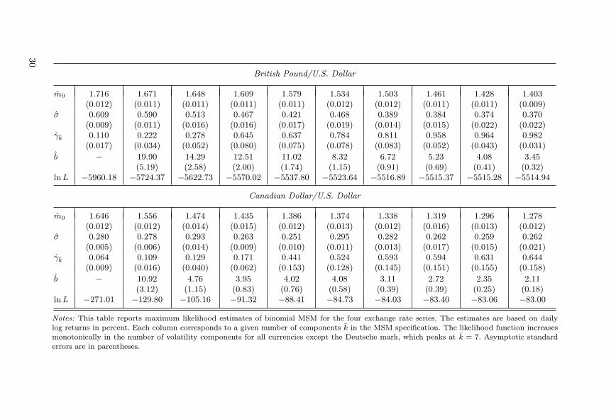
Notes: This table reports maximum likelihood estimates of binomial MSM for the four exchange rate series. The estimates are based on dailylog returns in percent. Each column corresponds to a given number of components k in the MSM specification. The likelihood function increasesmonotonically in the number of volatility components for all currencies except the Deutsche mark, which peaks at k = 7. Asymptotic standarderrors are in parentheses.

30

3.3 Empirical Results 31

We begin by examining the DM data. The multiplier parameter m0 tendsto decline with k because with a larger number of components, less variabil-ity is required in each Mk,t to match the fluctuations in volatility exhibitedby the data. The estimates of σ vary across k with no particular pattern.Standard errors of σ increase with k, consistent with the idea that long-runaverages are difficult to identify in models permitting long volatility cycles.We next examine the frequency parameters γk and b. When k = 1, the sin-gle multiplier has a duration slightly lower than two weeks. As k increases,the switching probability of the highest frequency multiplier increases untila switch occurs about once a day for large k. At the same time, the esti-mate b decreases steadily with k. When k = 10, we infer from (3.2) thatthe lowest frequency multiplier has a duration approximately equal to tenyears, or about one-third the sample size. Thus, as k increases, the rangeof frequencies spreads out, while the spacing between frequencies becomestighter.

The other currencies generate parameter estimates with similar proper-ties. In all cases, m0 tends to decrease with k. The values of m0, and thus theimportance of stochastic volatility, are largest for JA and UK and smallestfor CA. Variability across k in the estimates of σ is also greatest for JA andUK and least for CA. As k increases, the most transitory multiplier switchesmore often and the spacing between frequencies becomes tighter for all cur-rencies. The most persistent multiplier has the longest duration for the yen atapproximately three times the sample size and the smallest for the Canadiandollar at approximately one-tenth the sample size.

For large k, the estimated MSM(k)

processes generate substantial out-liers despite having finite moments of every order. For each currency, weuse the estimated process with k = 10 frequencies to generate ten thousandpaths of the same length as the data, and we compute a Hill (1975) tailindex α for each simulated path.5 Basing the index on 100 order statistics,the empirical tail index and the average α in the simulated samples are,respectively, equal to 4.74 and 4.34 (DM), 3.91 and 3.75 (JA), 4.59 and 4.03

5The tail index measures the rate of decline in the extremes of a distribution. For

example, given a Paretian tail satisfying P (X > x) ∼ kx−α for large x, the characteristicexponent, or tail index, is α, and only moments of order up to α are finite. If Xn1 ≤Xn2 ≤ . . . ≤ Xnn are the order statistics of {Xt}n

t=1 in ascending order, then Hill’s(1975) tail estimator is

αs =

⎛⎝1

s

s∑j=1

ln Xn,n−j+1 − ln Xn,n−s

⎞⎠

−1

.

This estimator is consistent and asympotically normal (Hall, 1982). Related estimatorsof the tail index are proposed by Pickands (1975) and de Haan and Resnick (1980).Applications in finance and extensions include Gabaix et al. (2003, 2006), Hols and deVries (1991), Jansen and de Vries (1991), Kearns and Pagan (1997), Loretan and Phillips(1994), Quintos, Fan, and Phillips (2001), and Wagner and Marsh (2005).

32 3. The Markov-Switching Multifractal (MSM) in Discrete Time

(UK), and 4.40 and 4.79 (CA). Furthermore, for all currencies we cannot atthe 10% level reject equality of the simulated and empirical tail statistics.This result is caused by the variations in volatility in the estimated models.The distribution of returns in MSM is a mixture of Gaussians, which hasfinite moments of every order. With the highest frequency multipliers tak-ing new values almost daily, this mixture appears to be more than sufficientto capture the tail characteristics of the data, even in a sample containingthirty years of daily observations.6

We finally examine the behavior of the log-likelihood function as thenumber of frequencies k increases from 1 to 10. For each currency, thelikelihood goes up substantially at low k and in most cases continues toincrease at a decreasing rate. The only exception to the monotonic increasein likelihood occurs in the DM series, for which the likelihood reaches a peakat k = 7. In all other cases, the likelihood reaches a maximum at k = 10.This behavior of the likelihood confirms that fluctuations in volatility occurwith heterogeneous degrees of persistence, and explicitly incorporating alarger number of frequencies results in a better fit.

3.3.3 Model SelectionWe now examine the statistical significance of the differences in likelihoodsacross estimated MSM(k) processes. Consider two models MSM(k) andMSM(k′), k = k′, with respective densities f and g. The processes arenonnested and have log-likelihood difference:

√T (lnLf

T − lnLgT ) =

1√T

T∑

t=1

lnf(rt |r1, . . . , rt−1 )g(rt |r1, . . . , rt−1 )

.

Consider the null hypothesis that the models have identical unconditionalexpected log-likelihoods. When the observations {rt} are i.i.d., Vuong (1989)shows that the difference ln Lf

T − lnLgT is asymptotically normal under the

null. In addition, the variance of this difference is consistently estimated bythe sample variance of the addends ln[f(rt |r1, . . . , rt−1 )/g(rt |r1, . . . , rt−1 )].Since the observations {rt} are typically not i.i.d. in financial applications,in the Appendix we construct a heteroskedasticity and autocorrelation con-sistent (HAC) version of the Vuong test. Our discussion is a simplified versionof the broader approach proposed by Rivers and Vuong (2002).

For each k ∈ {1, . . . , 9}, we test in Table 3.3 the null hypothesis thatMSM(k) and MSM(10) fit the data equally well. Since HAC-adjusted

6An extensive literature investigates the close connection between mixtures and fat

tails. For instance, Student and Cauchy distributions can be represented as mixtures ofnormals (e.g., Andrews and Mallows, 1974; Blattberg and Gonedes, 1974; Praetz, 1972),and the distinction between mixtures and Paretian distributions is therefore difficult tomake in practice (e.g., Kon, 1984). Furthermore, MSM mimics long-memory behavior,which impacts tail index estimation (e.g., Kearns and Pagan, 1997).

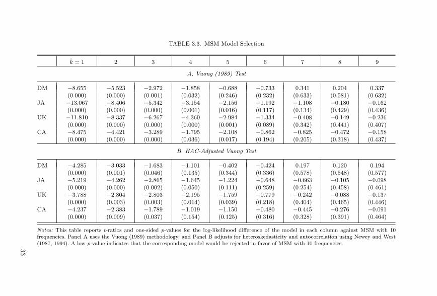
TABLE 3.3. MSM Model Selection

k = 1 2 3 4 5 6 7 8 9

A. Vuong (1989) Test

DM −8.655 −5.523 −2.972 −1.858 −0.688 −0.733 0.341 0.204 0.337(0.000) (0.000) (0.001) (0.032) (0.246) (0.232) (0.633) (0.581) (0.632)

JA −13.067 −8.406 −5.342 −3.154 −2.156 −1.192 −1.108 −0.180 −0.162(0.000) (0.000) (0.000) (0.001) (0.016) (0.117) (0.134) (0.429) (0.436)

UK −11.810 −8.337 −6.267 −4.360 −2.984 −1.334 −0.408 −0.149 −0.236(0.000) (0.000) (0.000) (0.000) (0.001) (0.089) (0.342) (0.441) (0.407)

CA −8.475 −4.421 −3.289 −1.795 −2.108 −0.862 −0.825 −0.472 −0.158(0.000) (0.000) (0.000) (0.036) (0.017) (0.194) (0.205) (0.318) (0.437)

B. HAC-Adjusted Vuong Test

DM −4.285 −3.033 −1.683 −1.101 −0.402 −0.424 0.197 0.120 0.194(0.000) (0.001) (0.046) (0.135) (0.344) (0.336) (0.578) (0.548) (0.577)

JA −5.219 −4.262 −2.865 −1.645 −1.224 −0.648 −0.663 −0.105 −0.098(0.000) (0.000) (0.002) (0.050) (0.111) (0.259) (0.254) (0.458) (0.461)

UK −3.788 −2.804 −2.803 −2.195 −1.759 −0.779 −0.242 −0.088 −0.137(0.000) (0.003) (0.003) (0.014) (0.039) (0.218) (0.404) (0.465) (0.446)

CA −4.237 −2.383 −1.789 −1.019 −1.150 −0.480 −0.445 −0.276 −0.091(0.000) (0.009) (0.037) (0.154) (0.125) (0.316) (0.328) (0.391) (0.464)

Notes: This table reports t-ratios and one-sided p-values for the log-likelihood difference of the model in each column against MSM with 10frequencies. Panel A uses the Vuong (1989) methodology, and Panel B adjusts for heteroskedasticity and autocorrelation using Newey and West(1987, 1994). A low p-value indicates that the corresponding model would be rejected in favor of MSM with 10 frequencies.

33

34 3. The Markov-Switching Multifractal (MSM) in Discrete Time

tests tend to perform poorly in small samples,7 we compute t-ratios andone-sided p-values using both the original and the HAC-adjusted methods.For k ∈ {1, 2, 3}, the log-likelihood difference is significant at the 1% levelin the nonadjusted case (Table 3.3A) and at the 5% level in the HAC case(Table 3.3B). This represents strong evidence that MSM(10) significantlyoutperforms models with one to three frequencies. For k ∈ {4, 5}, we rejectthe null at the 5% (nonadjusted) and 20% (HAC-adjusted) levels in almostall cases. These results provide substantial evidence that MSM(10) out-performs models with four or five frequencies. Lower significance levels areobtained for larger values of k, and the overall conclusion is that MSMworks better for larger numbers of frequencies. For this reason and for con-sistency in the remaining analysis, we henceforth focus on the MSM(k = 10)process for all currencies.

3.4 Comparison with Alternative Models

We now compare the multifractal model with GARCH(1,1) and Markov-switching GARCH, which are among the best traditional models forvolatility forecasting. The multifractal is then compared with fractionallyintegrated GARCH in order to assess the connection between long memoryand forecasting performance.

The alternative processes have the form rt = h1/2t εt, where ht is the

conditional variance of rt at date t − 1, and {εt} are i.i.d. Student innova-tions with unit variance and ν degrees of freedom. GARCH(1,1) assumesthe recursion ht+1 = ω + αr2

t + βht, as described in Chapter 2. MS-GARCH combines short-run autoregressive dynamics with low-frequencyregime shifts. A latent state st ∈ {1, 2} follows a first-order Markov processwith transition probabilities

pij = P (st+1 = j| st = i) .

In every period, the econometrician observes the return rt but not thelatent st. For i = {1, 2}, let ht+1(i) = V art(rt+1|st+1 = i) be the varianceof rt+1 conditional on st+1 = i and past returns {rs}t

s=1. The quantityht is latent in every period, and the econometrician can similarly defineEt [ht(st) |st+1 = i ] , the expectation of ht conditional on st+1 = i and pastreturns. Klaassen (2002) assumes the conditional dynamics:

ht+1(i) = ωi + αir2t + βiEt [ht(st) |st+1 = i ] . (3.6)

Klaassen shows that this model provides better forecasts for three of theexchange rates considered in this chapter (DM, JA, and UK) than the

7See, for example, Andrews (1991), Andrews and Monahan (1992), and den Haan

and Levin (1997).

3.4 Comparison with Alternative Models 35

earlier Markov-Switching GARCH formulation of Gray (1996), and alsopermits analytical multistep forecasting.

3.4.1 In-Sample ComparisonTable 3.4 presents the ML estimates of GARCH and MS-GARCH. Thecoefficient 1/ν is the inverse of the degrees of freedom in the Student dis-tribution. Each coefficient σi, i = 1, 2, represents the standard deviation ofreturns conditional on the volatility state: σ2

i = ωi/(1 − αi − βi).Table 3.5 shows that MSM has a higher likelihood than GARCH for

all exchange rates, even though both processes have the same number ofparameters. MS-GARCH uses nine parameters as compared to four witheither GARCH or MSM. Using the Schwarz BIC criterion to adjust for thisdifference, the multifractal model is indistinguishable from MS-GARCH inthe UK data and is preferred for DM and CA.

As suggested by Vuong (1989), we evaluate the statistical significanceof BIC differences. The last two columns of Table 3.5 test the alterna-tive models against MSM under this metric.8 We again give p-values forboth the original version of the test and a HAC-adjusted variant. For thestandard test, the in-sample performance of MSM over GARCH is highlysignificant for the mark, the yen, and the pound, and somewhat signifi-cant for the Canadian dollar. The HAC adjustments produce analogousbut slightly weaker results. Overall, the in-sample analysis suggests thatthe multifractal matches the performance MS-GARCH and significantlyoutperforms GARCH(1,1).

3.4.2 Out-of-Sample ForecastsWe now investigate the out-of-sample performance of the competing modelsover forecasting horizons ranging from 1 to 50 days. For each currency, weestimate the three processes on the beginning of the series, and we use thelast 12 years of data (or approximately half the sample) for out-of-samplecomparison.

In Table 3.6, we report the results for one-day forecasts. The first twocolumns correspond to the Mincer–Zarnowitz regressions of squared returnson their forecasts9:

r2t = γ0 + γ1Et−1(r2

t ) + ut.

8A BIC test of GARCH against the multifractal model is identical to a likelihood

test since both have the same number of parameters.9The forecasting regressions used by Mincer and Zarnowitz (1969) are common in

the financial econometrics literature. See, for instance, Andersen and Bollerslev (1998a),Andersen, Bollerslev, Diebold, and Labys (2003), Andersen, Bollerslev, and Meddahi(2005), Pagan and Schwert (1990), and West and Cho (1995).

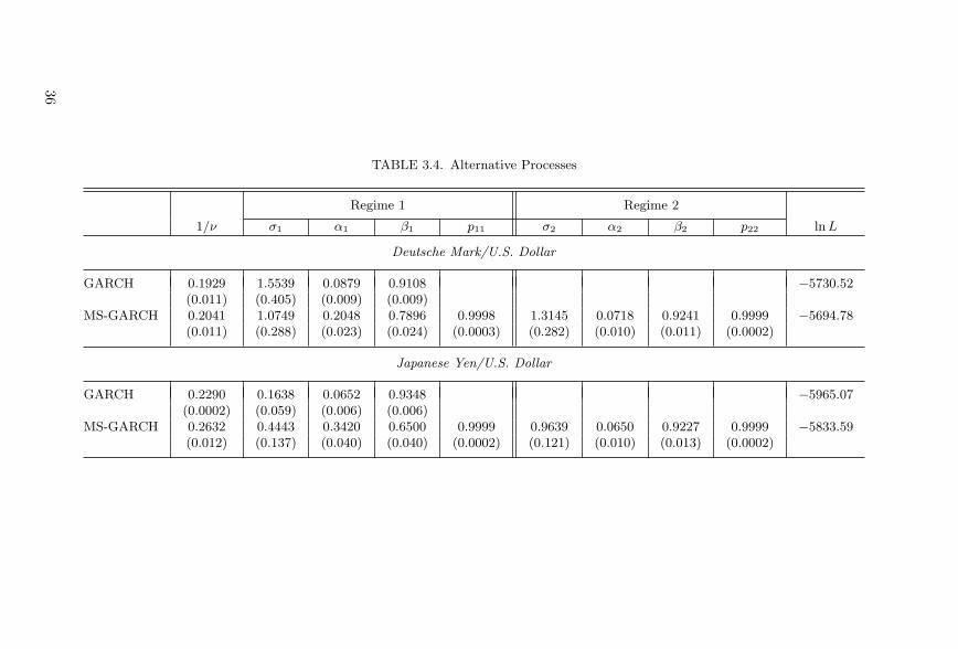
TABLE 3.4. Alternative Processes

Regime 1 Regime 2

1/ν σ1 α1 β1 p11 σ2 α2 β2 p22 ln L

Deutsche Mark/U.S. Dollar

GARCH 0.1929 1.5539 0.0879 0.9108 −5730.52(0.011) (0.405) (0.009) (0.009)

MS-GARCH 0.2041 1.0749 0.2048 0.7896 0.9998 1.3145 0.0718 0.9241 0.9999 −5694.78(0.011) (0.288) (0.023) (0.024) (0.0003) (0.282) (0.010) (0.011) (0.0002)

Japanese Yen/U.S. Dollar

GARCH 0.2290 0.1638 0.0652 0.9348 −5965.07(0.0002) (0.059) (0.006) (0.006)

MS-GARCH 0.2632 0.4443 0.3420 0.6500 0.9999 0.9639 0.0650 0.9227 0.9999 −5833.59(0.012) (0.137) (0.040) (0.040) (0.0002) (0.121) (0.010) (0.013) (0.0002)

36

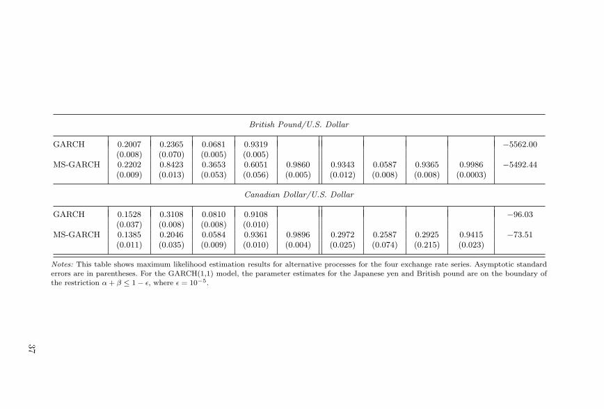
British Pound/U.S. Dollar

GARCH 0.2007 0.2365 0.0681 0.9319 −5562.00(0.008) (0.070) (0.005) (0.005)

MS-GARCH 0.2202 0.8423 0.3653 0.6051 0.9860 0.9343 0.0587 0.9365 0.9986 −5492.44(0.009) (0.013) (0.053) (0.056) (0.005) (0.012) (0.008) (0.008) (0.0003)

Canadian Dollar/U.S. Dollar

GARCH 0.1528 0.3108 0.0810 0.9108 −96.03(0.037) (0.008) (0.008) (0.010)

MS-GARCH 0.1385 0.2046 0.0584 0.9361 0.9896 0.2972 0.2587 0.2925 0.9415 −73.51(0.011) (0.035) (0.009) (0.010) (0.004) (0.025) (0.074) (0.215) (0.023)

Notes: This table shows maximum likelihood estimation results for alternative processes for the four exchange rate series. Asymptotic standarderrors are in parentheses. For the GARCH(1,1) model, the parameter estimates for the Japanese yen and British pound are on the boundary ofthe restriction α + β ≤ 1 − ε, where ε = 10−5.

37

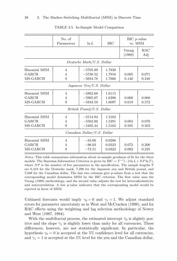
38 3. The Markov-Switching Multifractal (MSM) in Discrete Time

TABLE 3.5. In-Sample Model Comparison

No. of BIC p-valueParameters ln L BIC vs. MSM

Vuong HAC(1989) Adj

Deutsche Mark/U.S. Dollar

Binomial MSM 4 −5705.09 1.7830GARCH 4 −5730.52 1.7910 0.005 0.071MS-GARCH 9 −5694.78 1.7866 0.140 0.248

Japanese Yen/U.S. Dollar

Binomial MSM 4 −5862.68 1.6115GARCH 4 −5965.07 1.6396 0.000 0.008MS-GARCH 9 −5833.59 1.6097 0.619 0.572

British Pound/U.S. Dollar

Binomial MSM 4 −5514.94 1.5162GARCH 4 −5562.00 1.5291 0.004 0.070MS-GARCH 9 −5492.44 1.5162 0.505 0.503

Canadian Dollar/U.S. Dollar

Binomial MSM 4 −83.00 0.0286GARCH 4 −96.03 0.0323 0.072 0.200MS-GARCH 9 −73.51 0.0322 0.092 0.235

Notes: This table summarizes information about in-sample goodness of fit for the threemodels. The Bayesian Information Criterion is given by BIC = T −1(−2 ln L+NP ln T ),where NP is the number of free parameters in the specification. The sample lengths Tare 6,419 for the Deutsche mark, 7,298 for the Japanese yen and British pound, and7,048 for the Canadian dollar. The last two columns give p-values from a test that thecorresponding model dominates MSM by the BIC criterion. The first value uses theVuong (1989) methodology, and the second value adjusts the test for heteroskedasticityand autocorrelation. A low p-value indicates that the corresponding model would berejected in favor of MSM.

Unbiased forecasts would imply γ0 = 0 and γ1 = 1. We adjust standarderrors for parameter uncertainty as in West and McCracken (1998), and forHAC effects using the weighting and lag selection methodology of Neweyand West (1987, 1994).

With the multifractal process, the estimated intercept γ0 is slightly pos-itive and the slope γ1 is slightly lower than unity for all currencies. Thesedifferences, however, are not statistically significant. In particular, thehypothesis γ0 = 0 is accepted at the 5% confidence level for all currencies,and γ1 = 1 is accepted at the 5% level for the yen and the Canadian dollar,

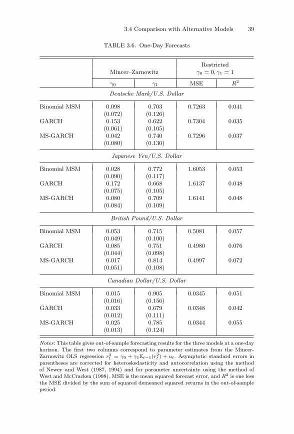
3.4 Comparison with Alternative Models 39

TABLE 3.6. One-Day Forecasts

RestrictedMincer–Zarnowitz γ0 = 0, γ1 = 1

γ0 γ1 MSE R2

Deutsche Mark/U.S. Dollar

Binomial MSM 0.098 0.703 0.7263 0.041(0.072) (0.126)

GARCH 0.153 0.622 0.7304 0.035(0.061) (0.105)

MS-GARCH 0.042 0.740 0.7296 0.037(0.080) (0.130)

Japanese Yen/U.S. Dollar

Binomial MSM 0.028 0.772 1.6053 0.053(0.090) (0.117)

GARCH 0.172 0.668 1.6137 0.048(0.075) (0.105)

MS-GARCH 0.080 0.709 1.6141 0.048(0.084) (0.109)

British Pound/U.S. Dollar

Binomial MSM 0.053 0.715 0.5081 0.057(0.049) (0.100)

GARCH 0.085 0.751 0.4980 0.076(0.044) (0.098)

MS-GARCH 0.017 0.814 0.4997 0.072(0.051) (0.108)

Canadian Dollar/U.S. Dollar

Binomial MSM 0.015 0.905 0.0345 0.051(0.016) (0.156)

GARCH 0.033 0.679 0.0348 0.042(0.012) (0.111)

MS-GARCH 0.025 0.785 0.0344 0.055(0.013) (0.124)

Notes: This table gives out-of-sample forecasting results for the three models at a one-dayhorizon. The first two columns correspond to parameter estimates from the Mincer-Zarnowitz OLS regression r2

t = γ0 + γ1Et−1(r2t ) + ut. Asymptotic standard errors in

parentheses are corrected for heteroskedasticity and autocorrelation using the methodof Newey and West (1987, 1994) and for parameter uncertainty using the method ofWest and McCracken (1998). MSE is the mean squared forecast error, and R2 is one lessthe MSE divided by the sum of squared demeaned squared returns in the out-of-sampleperiod.

40 3. The Markov-Switching Multifractal (MSM) in Discrete Time

and at the 1% level for the mark and the pound. The Mincer–Zarnowitzregressions show little evidence of bias in MSM forecasts.

The regression coefficients are slightly worse with GARCH(1,1). Inter-cepts are further away from zero for all currencies, and slopes are furtheraway from unity for three currencies. These biases are statistically signifi-cant. The hypotheses γ0 = 0 and γ1 = 1 are rejected at the 5% level in sevenout of eight cases. Since 0 < γ1 < 1, these results suggest that GARCHforecasts are too variable and can be improved by the linear smoothing ruleγ0 + γ1Et−1(r2

t ).Markov-switching GARCH improves on the out-of-sample performance

of GARCH(1,1). We accept that γ0 = 0 at the 5% confidence level for allcurrencies and that γ1 = 1 at the 1% level for DM, UK, and CA. Further-more, the regression estimates are best with MS-GARCH for two currencies(DM and UK) and with the multifractal for the other two. We also report inTable 3.6 two standard measures of goodness of fit: the mean squared error(MSE) and the restricted R2 coefficient.10 The multifractal produces thebest forecasting R2 for the mark and the yen. On the other hand, GARCHproduces better results for the pound and MS-GARCH for the Canadiandollar. To summarize the one-day forecast results, binomial MSM appearsto slightly dominate GARCH(1,1) and to produce results comparable toMS-GARCH.

Multistep forecasts provide stronger empirical differences between thethree models. Following Andersen and Bollerslev (1998a), the depen-dent variable is the sum of squared daily returns over n days, RVt,n =∑t

s=t−n+1 r2s . In Table 3.7, we report the results of the Mincer–Zarnowitz

regression:

RVt,n = γ0 + γ1Et−n (RVt,n) + ut

for n = 20 days. Because the average size of returns increases with thesampling interval, the estimated intercepts γ0 are larger in Table 3.7 thanin Table 3.6. For each currency, the multifractal produces point estimatesof γ0 and γ1 that are closest to their preferred values. We also accept thehypotheses γ0 = 0 and γ1 = 1 in all cases at the 5% confidence level.In contrast, for the other models each currency leads to a strong rejec-tion of either one hypothesis (MS-GARCH) or both (GARCH) at the 5%confidence level. The reported MSE and R2 further confirm that the multi-fractal provides the best 20-day forecasts for all currencies. The differenceis particularly large in the case of the DM and JA. The R2 coefficient is

10The mean squared error (MSE) quantifies the forecast errors in the out-of-sample

period: MSE = K−1 ∑Tt=T−K+1

(r2t − Et−1r2

t

)2, where K is the number of daysin the out-of-sample period. The out-of-sample coefficient of determination is R2 =1 − MSE/TSS, where TSS is the out-of-sample variance of squared returns: TSS =

K−1 ∑Tt=T−K+1

(r2t −

∑Ti=T−K+1 r2

i /K)2

.

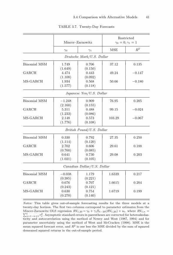
3.4 Comparison with Alternative Models 41

TABLE 3.7. Twenty-Day Forecasts

RestrictedMincer–Zarnowitz γ0 = 0, γ1 = 1

γ0 γ1 MSE R2

Deutsche Mark/U.S. Dollar

Binomial MSM 1.749 0.706 37.12 0.135(1.649) (0.150)

GARCH 4.474 0.443 49.24 −0.147(1.108) (0.092)

MS-GARCH 1.934 0.568 50.66 −0.180(1.577) (0.118)

Japanese Yen/U.S. Dollar

Binomial MSM −1.248 0.909 76.95 0.205(2.160) (0.155)

GARCH 5.311 0.488 99.15 −0.024(1.233) (0.086)

MS-GARCH 2.148 0.573 103.29 −0.067(1.776) (0.108)

British Pound/U.S. Dollar

Binomial MSM 0.330 0.792 27.35 0.250(1.114) (0.120)

GARCH 2.702 0.606 29.61 0.188(0.760) (0.085)

MS-GARCH 0.641 0.730 29.08 0.203(1.021) (0.105)

Canadian Dollar/U.S. Dollar

Binomial MSM −0.038 1.179 1.6339 0.217(0.385) (0.221)

GARCH 0.676 0.707 1.6615 0.204(0.243) (0.121)

MS-GARCH 0.630 0.754 1.6719 0.199(0.270) (0.140)

Notes: This table gives out-of-sample forecasting results for the three models at atwenty-day horizon. The first two columns correspond to parameter estimates from theMincer-Zarnowitz OLS regression RVt,20 = γ0 + γ1Et−20(RVt,20) + ut, where RVt,n =∑t

s=t−n+1 r2s . Asymptotic standard errors in parentheses are corrected for heteroskedas-

ticity and autocorrelation using the method of Newey and West (1987, 1994) and forparameter uncertainty using the method of West and McCracken (1998). MSE is themean squared forecast error, and R2 is one less the MSE divided by the sum of squareddemeaned squared returns in the out-of-sample period.

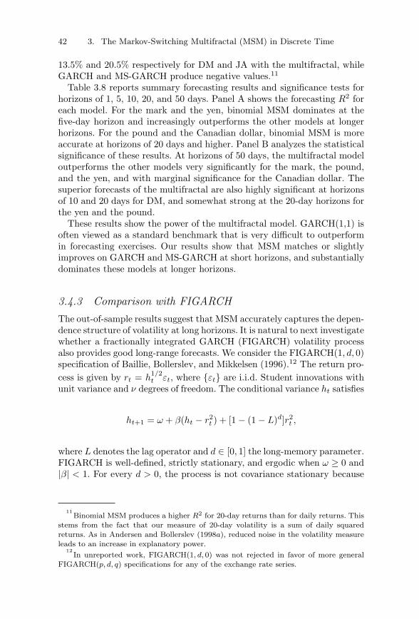
42 3. The Markov-Switching Multifractal (MSM) in Discrete Time

13.5% and 20.5% respectively for DM and JA with the multifractal, whileGARCH and MS-GARCH produce negative values.11

Table 3.8 reports summary forecasting results and significance tests forhorizons of 1, 5, 10, 20, and 50 days. Panel A shows the forecasting R2 foreach model. For the mark and the yen, binomial MSM dominates at thefive-day horizon and increasingly outperforms the other models at longerhorizons. For the pound and the Canadian dollar, binomial MSM is moreaccurate at horizons of 20 days and higher. Panel B analyzes the statisticalsignificance of these results. At horizons of 50 days, the multifractal modeloutperforms the other models very significantly for the mark, the pound,and the yen, and with marginal significance for the Canadian dollar. Thesuperior forecasts of the multifractal are also highly significant at horizonsof 10 and 20 days for DM, and somewhat strong at the 20-day horizons forthe yen and the pound.

These results show the power of the multifractal model. GARCH(1,1) isoften viewed as a standard benchmark that is very difficult to outperformin forecasting exercises. Our results show that MSM matches or slightlyimproves on GARCH and MS-GARCH at short horizons, and substantiallydominates these models at longer horizons.

3.4.3 Comparison with FIGARCHThe out-of-sample results suggest that MSM accurately captures the depen-dence structure of volatility at long horizons. It is natural to next investigatewhether a fractionally integrated GARCH (FIGARCH) volatility processalso provides good long-range forecasts. We consider the FIGARCH(1, d, 0)specification of Baillie, Bollerslev, and Mikkelsen (1996).12 The return pro-cess is given by rt = h

1/2t εt, where {εt} are i.i.d. Student innovations with

unit variance and ν degrees of freedom. The conditional variance ht satisfies

ht+1 = ω + β(ht − r2t ) + [1 − (1 − L)d]r2

t ,

where L denotes the lag operator and d ∈ [0, 1] the long-memory parameter.FIGARCH is well-defined, strictly stationary, and ergodic when ω ≥ 0 and|β| < 1. For every d > 0, the process is not covariance stationary because

11Binomial MSM produces a higher R2 for 20-day returns than for daily returns. This

stems from the fact that our measure of 20-day volatility is a sum of daily squaredreturns. As in Andersen and Bollerslev (1998a), reduced noise in the volatility measureleads to an increase in explanatory power.

12In unreported work, FIGARCH(1, d, 0) was not rejected in favor of more general

FIGARCH(p, d, q) specifications for any of the exchange rate series.

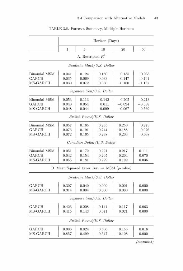
3.4 Comparison with Alternative Models 43

TABLE 3.8. Forecast Summary, Multiple Horizons

Horizon (Days)

1 5 10 20 50

A. Restricted R2

Deutsche Mark/U.S. Dollar

Binomial MSM 0.041 0.124 0.160 0.135 0.038GARCH 0.035 0.069 0.033 −0.147 −0.761MS-GARCH 0.039 0.072 0.030 −0.180 −1.137

Japanese Yen/U.S. Dollar

Binomial MSM 0.053 0.113 0.142 0.205 0.213GARCH 0.048 0.054 0.011 −0.024 −0.358MS-GARCH 0.048 0.044 −0.009 −0.067 −0.569

British Pound/U.S. Dollar

Binomial MSM 0.057 0.165 0.235 0.250 0.273GARCH 0.076 0.191 0.244 0.188 −0.026MS-GARCH 0.072 0.165 0.238 0.203 0.038

Canadian Dollar/U.S. Dollar

Binomial MSM 0.051 0.172 0.221 0.217 0.111GARCH 0.042 0.154 0.205 0.204 0.070MS-GARCH 0.055 0.181 0.229 0.199 0.036

B. Mean Squared Error Test vs. MSM (p-value)

Deutsche Mark/U.S. Dollar

GARCH 0.307 0.040 0.009 0.001 0.000MS-GARCH 0.314 0.004 0.000 0.000 0.000

Japanese Yen/U.S. Dollar

GARCH 0.426 0.208 0.144 0.117 0.063MS-GARCH 0.415 0.143 0.071 0.021 0.000

British Pound/U.S. Dollar

GARCH 0.906 0.824 0.606 0.156 0.016MS-GARCH 0.857 0.499 0.547 0.108 0.000

(continued)

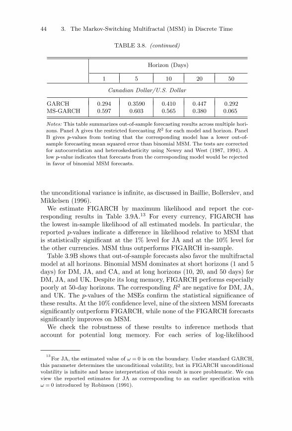
44 3. The Markov-Switching Multifractal (MSM) in Discrete Time

TABLE 3.8. (continued)

Horizon (Days)

1 5 10 20 50

Canadian Dollar/U.S. Dollar

GARCH 0.294 0.3590 0.410 0.447 0.292MS-GARCH 0.597 0.603 0.565 0.380 0.065

Notes: This table summarizes out-of-sample forecasting results across multiple hori-zons. Panel A gives the restricted forecasting R2 for each model and horizon. PanelB gives p-values from testing that the corresponding model has a lower out-of-sample forecasting mean squared error than binomial MSM. The tests are correctedfor autocorrelation and heteroskedasticity using Newey and West (1987, 1994). Alow p-value indicates that forecasts from the corresponding model would be rejectedin favor of binomial MSM forecasts.

the unconditional variance is infinite, as discussed in Baillie, Bollerslev, andMikkelsen (1996).

We estimate FIGARCH by maximum likelihood and report the cor-responding results in Table 3.9A.13 For every currency, FIGARCH hasthe lowest in-sample likelihood of all estimated models. In particular, thereported p-values indicate a difference in likelihood relative to MSM thatis statistically significant at the 1% level for JA and at the 10% level forthe other currencies. MSM thus outperforms FIGARCH in-sample.

Table 3.9B shows that out-of-sample forecasts also favor the multifractalmodel at all horizons. Binomial MSM dominates at short horizons (1 and 5days) for DM, JA, and CA, and at long horizons (10, 20, and 50 days) forDM, JA, and UK. Despite its long memory, FIGARCH performs especiallypoorly at 50-day horizons. The corresponding R2 are negative for DM, JA,and UK. The p-values of the MSEs confirm the statistical significance ofthese results. At the 10% confidence level, nine of the sixteen MSM forecastssignificantly outperform FIGARCH, while none of the FIGARCH forecastssignificantly improves on MSM.

We check the robustness of these results to inference methods thataccount for potential long memory. For each series of log-likelihood

13For JA, the estimated value of ω = 0 is on the boundary. Under standard GARCH,

this parameter determines the unconditional volatility, but in FIGARCH unconditionalvolatility is infinite and hence interpretation of this result is more problematic. We canview the reported estimates for JA as corresponding to an earlier specification withω = 0 introduced by Robinson (1991).

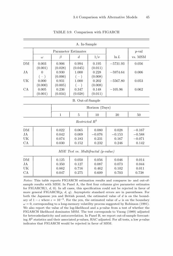
3.4 Comparison with Alternative Models 45

TABLE 3.9. Comparison with FIGARCH

A. In-Sample

Parameter Estimates p-val

ω β d 1/ν ln L vs. MSM

DM 0.003 0.906 0.994 0.195 −5731.93 0.056(0.001) (0.028) (0.045) (0.011)

JA 0 0.930 1.000 0.228 −5974.64 0.006( – ) (0.006) ( – ) (0.008)

UK 0.000 0.931 1.000 0.202 −5567.80 0.053(0.000) (0.005) ( – ) (0.008)

CA 0.005 0.236 0.347 0.148 −105.96 0.062(0.001) (0.034) (0.028) (0.011)

B. Out-of-Sample

Horizon (Days)

1 5 10 20 50

Restricted R2

DM 0.022 0.065 0.080 0.028 −0.167JA 0.042 0.009 −0.076 −0.153 −0.588UK 0.074 0.183 0.231 0.167 −0.071CA 0.030 0.152 0.232 0.246 0.142

MSE Test vs. Multifractal (p-value)

DM 0.125 0.050 0.056 0.046 0.014JA 0.350 0.127 0.087 0.073 0.044UK 0.882 0.716 0.462 0.102 0.011CA 0.047 0.275 0.609 0.703 0.738

Notes: This table reports FIGARCH estimation results and compares in- and out-of-sample results with MSM. In Panel A, the first four columns give parameter estimatesfor FIGARCH(1, d, 0). In all cases, this specification could not be rejected in favor ofmore general FIGARCH(p, d, q). Asymptotic standard errors are in parentheses. Forboth the Japanese yen and British pound, the estimated value of d is on the bound-ary of 1 − ε where ε = 10−5. For the yen, the estimated value of ω is on the boundaryω = 0, corresponding to a long-memory volatility process suggested by Robinson (1991).We also report the value of the log-likelihood and a p-value from a test of whether theFIGARCH likelihood dominates MSM. The test corresponds to Vuong (1989) adjustedfor heteroskedasticity and autocorrelation. In Panel B, we report out-of-sample forecast-ing R2 statistics and their associated p-values, HAC adjusted. For all tests, a low p-valueindicates that FIGARCH would be rejected in favor of MSM.

46 3. The Markov-Switching Multifractal (MSM) in Discrete Time

differences, we calculate local Whittle estimates14 of d and obtain values ofapproximately −0.08 for DM, 0.08 for JA, −0.05 for UK and 0.09 for CA.15

These statistics are insignificant or marginally significant. We then use thememory autocorrelation consistent (MAC) estimation method developedby Peter Robinson (2005) to calculate alternative variance estimates forthe log-likelihood differences and assess statistical significance.16 Thesep-values are respectively equal to 0.0001 (DM), 0.015 (JA), 0.01 (UK)and 0.077 (CA), again suggesting that the MSM outperforms FIGARCHin-sample. We similarly check robustness of the MSE difference testsreported in Panel B to MAC adjustment, and find moderate attenuation oft-statistics and movement of p-values toward 0.5 for long horizons. Overall,the results reported in this section support the good performance of MSMrelative to FIGARCH both in- and out-of-sample.

3.5 Discussion

This chapter presents the Markov-Switching Multifractal, which suggestsan expanded role for regime-switching in volatility modeling. Traditionalregime-switching approaches such as MS-GARCH augment low-frequencyswitches with midrange GARCH transitions and a thick-tailed conditionaldistribution of returns. By contrast, MSM effectively captures the rele-vant empirical features of financial data at all horizons with the singlemechanism of multifrequency regime-switching.

The original research on which this chapter is based showed for thefirst time how to use standard econometric tools to estimate multifrac-tal processes with confidence intervals on parameters, test hypotheses, andconduct multistep volatility forecasting. We compare the performance ofthe multifractal model with leading volatility models such as GARCH,MS-GARCH, and FIGARCH. Like MSM, these models conveniently per-mit maximum likelihood estimation and analytical forecasting. In-sample,binomial MSM has significantly higher likelihood than either GARCH orFIGARCH even though these processes have the same number of param-eters. Out-of-sample, MSM matches or outperforms all three comparison

14The local Whittle estimator of d was proposed and developed by Kunsch (1987) and

Robinson (1995b). Additional contributions on the asymptotic properties of the estima-tor, modifications, and discussions of robustness under alternative specifications of longmemory include Hurvich and Chen (2000), Phillips (1999), Phillips and Shimotsu (2004),Shimotsu and Phillips (2005, 2006), and Velasco (1999). The long-memory parameter dmay also be estimated by log periodogram regression (Geweke and Porter-Hudak, 1983;Robinson, 1995a; Hurvich, Deo, and Brodsky, 1998; Andrews and Guggenberger, 2003).

15We use a bandwidth equal to T 0.6 in all of our estimates.

16Abadir, Distaso, and Giraitis (2008) provide a detailed assessment of the asymptotic

properties and robustness of the MAC estimator.

3.5 Discussion 47

models at short horizons and substantially dominates at 20- to 50-dayhorizons. The recent study by Lux (2008) confirms many of these findings.

Researchers often focus on applications of immediate practical valuewhen assessing statistical models. Correspondingly, this chapter has shownthat MSM performs well by several standard metrics. In the remainder ofthis book, we show that MSM extends easily to multivariate applications,generalizes naturally to continuous time while capturing the power varia-tions exhibited by many financial series, and incorporates productively intoexisting asset pricing frameworks in both discrete and continuous time.

4Multivariate MSM

Joint movements in volatility across asset markets influence the distributionof returns at the portfolio level and therefore play an important role in riskmanagement, portfolio selection, and derivative pricing. Comovements involatility also help our understanding of financial markets and shed lighton issues such as contagion and the transmission of shocks through thefinancial system (e.g., Engle, Ito, and Lin, 1990).

This chapter begins by investigating possible linkages between the MSMvolatility components of three currencies and several macroeconomic andfinancial indicators over the 1973–2003 period. We find no robust patternbetween MSM components and variables such as inflation, money supply,interest rates, industrial production, and stock market volatility. On theother hand, oil and gold prices both correlate positively with currencyvolatility over the past three decades, consistent with the view that thesecommodities may act as proxies for global economic and political risk.

Across currency pairs, volatility components from different series withsimilar frequencies tend to move together, while components with verydifferent frequencies display less correlation. These findings motivate theconstruction of a bivariate model of volatility. This specification, calledbivariate MSM, is parsimonious as the number of parameters is independentof k. Positive semidefiniteness of the covariance matrix is guaranteed byconstruction. Furthermore, the likelihood function can be written in closedform, and maximum likelihood estimation can be implemented for relativelysmall state spaces. To accommodate a large number of frequencies, wedevelop a particle filter that permits convenient inference and forecastingusing simulations. Monte Carlo experiments confirm the good performanceof this approach, which broadens the range of computationally tractableMSM specifications.

We estimate the bivariate model by maximum likelihood, and we verifythat the goodness of fit increases with the number of volatility components.Likelihood ratio tests also confirm that the main assumptions of the modelare empirically valid. Bivariate MSM compares favorably to constant cor-relation GARCH (CC-GARCH) in-sample. Out-of-sample, bivariate MSMcaptures well the conditional distribution of a variety of currency portfoliosand provides reasonable measures of value-at-risk.

This chapter is based on an earlier paper: “Volatility Comovement: A MultifrequencyApproach” (with A. Fisher and S. Thompson), Journal of Econometrics, 131: 179–215,March 2006.

50 4. Multivariate MSM

4.1 Comovement of Univariate VolatilityComponents

4.1.1 Comovement of Exchange Rate VolatilityThe empirical analysis investigates daily returns on the Deutsche mark(DM), Japanese yen (JA), and British pound (UK), all against theU.S. dollar. As in Chapter 3, the returns are imputed from noon dailyprices reported by the Federal Reserve Bank of New York. The Deutschemark is spliced with the euro at the beginning of 1999. Each series runsbetween 1 June 1973 and 30 October 2003, and contains 7,635 observations.

For each currency, we estimate MSM by maximum likelihood on theentire sample, and we report the results in Table 4.1. These univariateresults are similar to those reported in Chapter 3 even though the sampleused for ML estimation is slightly longer.

Using the ML estimates, we compute for each currency the smoothedstate probabilities P

(Mt = mj |r1, . . . , rT

)as in Kim (1994).1 We also cal-

culate the expectation of the individual multipliers conditional on the entiresample:

Mk,t = E(Mk,t|r1, . . . , rT ) (4.1)

and report in Table 4.2 the correlations of the smoothed components Mk,t.The first panel shows that different components of the DM series aremoderately correlated, and correlation decreases in the distance betweenfrequencies.2 Untabulated results for the pound and yen series are similar.The second and third panels of Table 4.2 show comovement of the markcomponents with the yen and the pound. Correlation between the smoothedbeliefs Mα

k,t and Mβk′,t of two currencies tends to be high when k and

k′ are close, and low otherwise. This suggests that the volatility compo-nents of two exchange rates are most correlated when their frequencies aresimilar.

The interpretation is slightly complicated by the fact that the set ofvolatility frequencies is not identical across currencies. To address this issue,we introduce a simple bivariate model in which currencies are statisticallyindependent but have identical frequency parameters b and γk. The log-likelihood of the two series is

L(rαt ;mα

0 , σα, b, γk) + L(rβt ;mβ

0 , σβ , b, γk), (4.2)

1The smoothed state probabilities (4.1) are conditioned on all available data, while

the filtered probabilities given in equation (3.4) are based only on information availableup to date t. See Hamilton (1994) for further discussion.

2Since the econometrician does not directly observe the multipliers, correlation in

smoothed beliefs is not inconsistent with the assumed independence of the unobservedcomponents Mk,t and Mk′,t, k �= k′.

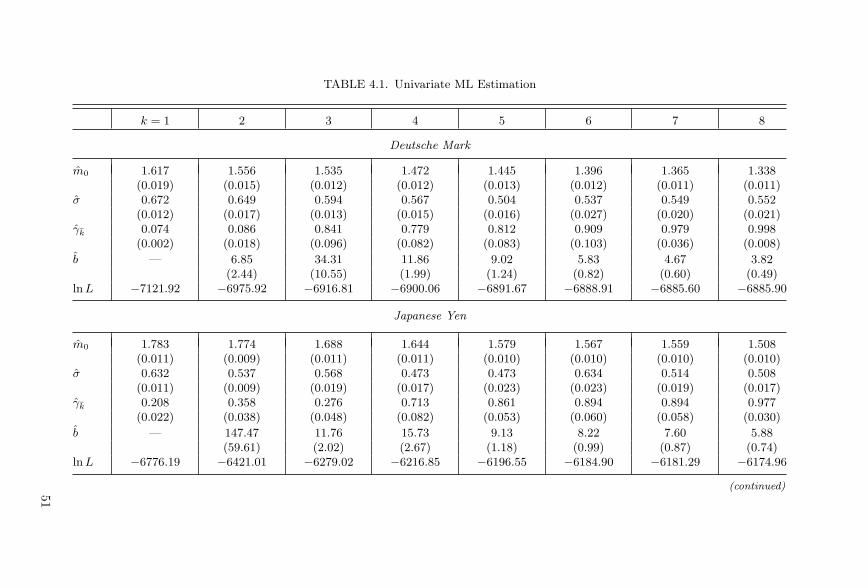
TABLE 4.1. Univariate ML Estimation

k = 1 2 3 4 5 6 7 8

Deutsche Mark

m0 1.617 1.556 1.535 1.472 1.445 1.396 1.365 1.338(0.019) (0.015) (0.012) (0.012) (0.013) (0.012) (0.011) (0.011)

σ 0.672 0.649 0.594 0.567 0.504 0.537 0.549 0.552(0.012) (0.017) (0.013) (0.015) (0.016) (0.027) (0.020) (0.021)

γk 0.074 0.086 0.841 0.779 0.812 0.909 0.979 0.998(0.002) (0.018) (0.096) (0.082) (0.083) (0.103) (0.036) (0.008)

b — 6.85 34.31 11.86 9.02 5.83 4.67 3.82(2.44) (10.55) (1.99) (1.24) (0.82) (0.60) (0.49)

ln L −7121.92 −6975.92 −6916.81 −6900.06 −6891.67 −6888.91 −6885.60 −6885.90

Japanese Yen

m0 1.783 1.774 1.688 1.644 1.579 1.567 1.559 1.508(0.011) (0.009) (0.011) (0.011) (0.010) (0.010) (0.010) (0.010)

σ 0.632 0.537 0.568 0.473 0.473 0.634 0.514 0.508(0.011) (0.009) (0.019) (0.017) (0.023) (0.023) (0.019) (0.017)

γk 0.208 0.358 0.276 0.713 0.861 0.894 0.894 0.977(0.022) (0.038) (0.048) (0.082) (0.053) (0.060) (0.058) (0.030)

b — 147.47 11.76 15.73 9.13 8.22 7.60 5.88(59.61) (2.02) (2.67) (1.18) (0.99) (0.87) (0.74)

ln L −6776.19 −6421.01 −6279.02 −6216.85 −6196.55 −6184.90 −6181.29 −6174.96

(continued)51

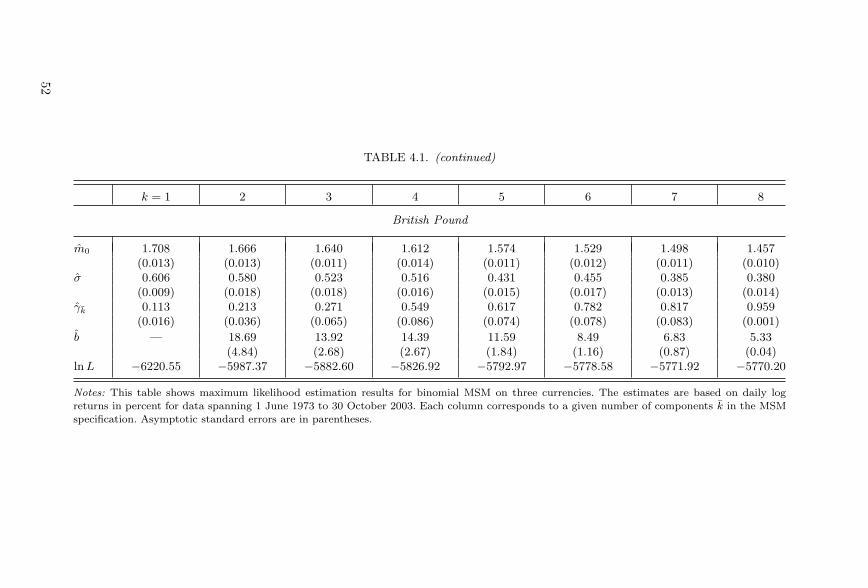
TABLE 4.1. (continued)

k = 1 2 3 4 5 6 7 8

British Pound

m0 1.708 1.666 1.640 1.612 1.574 1.529 1.498 1.457(0.013) (0.013) (0.011) (0.014) (0.011) (0.012) (0.011) (0.010)

σ 0.606 0.580 0.523 0.516 0.431 0.455 0.385 0.380(0.009) (0.018) (0.018) (0.016) (0.015) (0.017) (0.013) (0.014)

γk 0.113 0.213 0.271 0.549 0.617 0.782 0.817 0.959(0.016) (0.036) (0.065) (0.086) (0.074) (0.078) (0.083) (0.001)

b — 18.69 13.92 14.39 11.59 8.49 6.83 5.33(4.84) (2.68) (2.67) (1.84) (1.16) (0.87) (0.04)

ln L −6220.55 −5987.37 −5882.60 −5826.92 −5792.97 −5778.58 −5771.92 −5770.20

Notes: This table shows maximum likelihood estimation results for binomial MSM on three currencies. The estimates are based on daily logreturns in percent for data spanning 1 June 1973 to 30 October 2003. Each column corresponds to a given number of components k in the MSMspecification. Asymptotic standard errors are in parentheses.

52

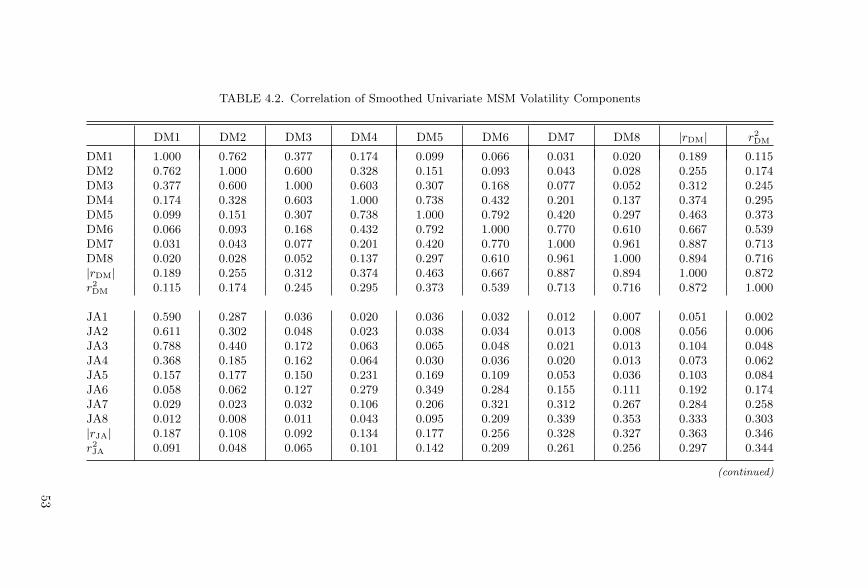
TABLE 4.2. Correlation of Smoothed Univariate MSM Volatility Components

DM1 DM2 DM3 DM4 DM5 DM6 DM7 DM8 |rDM| r2DM

DM1 1.000 0.762 0.377 0.174 0.099 0.066 0.031 0.020 0.189 0.115DM2 0.762 1.000 0.600 0.328 0.151 0.093 0.043 0.028 0.255 0.174DM3 0.377 0.600 1.000 0.603 0.307 0.168 0.077 0.052 0.312 0.245DM4 0.174 0.328 0.603 1.000 0.738 0.432 0.201 0.137 0.374 0.295DM5 0.099 0.151 0.307 0.738 1.000 0.792 0.420 0.297 0.463 0.373DM6 0.066 0.093 0.168 0.432 0.792 1.000 0.770 0.610 0.667 0.539DM7 0.031 0.043 0.077 0.201 0.420 0.770 1.000 0.961 0.887 0.713DM8 0.020 0.028 0.052 0.137 0.297 0.610 0.961 1.000 0.894 0.716|rDM| 0.189 0.255 0.312 0.374 0.463 0.667 0.887 0.894 1.000 0.872r2DM 0.115 0.174 0.245 0.295 0.373 0.539 0.713 0.716 0.872 1.000

JA1 0.590 0.287 0.036 0.020 0.036 0.032 0.012 0.007 0.051 0.002JA2 0.611 0.302 0.048 0.023 0.038 0.034 0.013 0.008 0.056 0.006JA3 0.788 0.440 0.172 0.063 0.065 0.048 0.021 0.013 0.104 0.048JA4 0.368 0.185 0.162 0.064 0.030 0.036 0.020 0.013 0.073 0.062JA5 0.157 0.177 0.150 0.231 0.169 0.109 0.053 0.036 0.103 0.084JA6 0.058 0.062 0.127 0.279 0.349 0.284 0.155 0.111 0.192 0.174JA7 0.029 0.023 0.032 0.106 0.206 0.321 0.312 0.267 0.284 0.258JA8 0.012 0.008 0.011 0.043 0.095 0.209 0.339 0.353 0.333 0.303|rJA| 0.187 0.108 0.092 0.134 0.177 0.256 0.328 0.327 0.363 0.346r2JA 0.091 0.048 0.065 0.101 0.142 0.209 0.261 0.256 0.297 0.344

(continued)

53

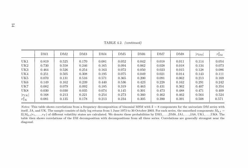
TABLE 4.2. (continued)

DM1 DM2 DM3 DM4 DM5 DM6 DM7 DM8 |rDM| r2DM

UK1 0.819 0.525 0.170 0.081 0.052 0.042 0.018 0.011 0.114 0.054UK2 0.730 0.558 0.246 0.165 0.094 0.062 0.028 0.018 0.134 0.073UK3 0.464 0.526 0.254 0.163 0.072 0.050 0.023 0.015 0.128 0.086UK4 0.251 0.505 0.308 0.195 0.075 0.049 0.021 0.014 0.143 0.111UK5 0.070 0.131 0.516 0.571 0.365 0.200 0.091 0.062 0.213 0.169UK6 0.149 0.162 0.239 0.440 0.536 0.423 0.228 0.162 0.291 0.242UK7 0.082 0.079 0.092 0.185 0.319 0.463 0.431 0.362 0.407 0.354UK8 0.030 0.030 0.035 0.074 0.145 0.301 0.473 0.488 0.471 0.409|rUK| 0.168 0.213 0.221 0.254 0.273 0.360 0.462 0.462 0.564 0.524r2UK 0.081 0.135 0.178 0.213 0.234 0.305 0.390 0.391 0.508 0.571

Notes: This table shows correlations from a frequency decomposition of binomial MSM with k = 8 components for the univariate DM series withitself, JA, and UK. The sample consists of daily log returns from 1 June 1973 to 30 October 2003. For each series, the smoothed components Mk,t =E(Mk,t|r1, . . . , rT ) of different volatility states are calculated. We denote these probabilities by DM1, . . . ,DM8, JA1, . . . ,JA8, UK1, . . . ,UK8. Thetable then shows correlations of the DM decomposition with decompositions from all three series. Correlations are generally strongest near thediagonal.

54

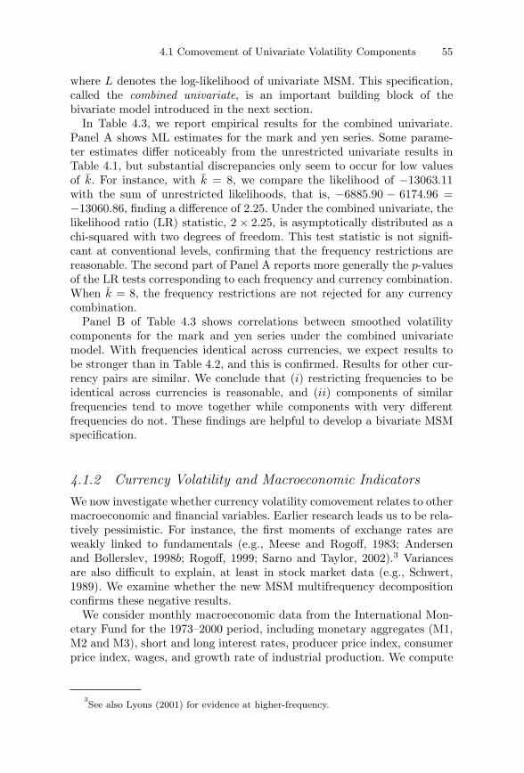
4.1 Comovement of Univariate Volatility Components 55

where L denotes the log-likelihood of univariate MSM. This specification,called the combined univariate, is an important building block of thebivariate model introduced in the next section.

In Table 4.3, we report empirical results for the combined univariate.Panel A shows ML estimates for the mark and yen series. Some parame-ter estimates differ noticeably from the unrestricted univariate results inTable 4.1, but substantial discrepancies only seem to occur for low valuesof k. For instance, with k = 8, we compare the likelihood of −13063.11with the sum of unrestricted likelihoods, that is, −6885.90 − 6174.96 =−13060.86, finding a difference of 2.25. Under the combined univariate, thelikelihood ratio (LR) statistic, 2 × 2.25, is asymptotically distributed as achi-squared with two degrees of freedom. This test statistic is not signifi-cant at conventional levels, confirming that the frequency restrictions arereasonable. The second part of Panel A reports more generally the p-valuesof the LR tests corresponding to each frequency and currency combination.When k = 8, the frequency restrictions are not rejected for any currencycombination.

Panel B of Table 4.3 shows correlations between smoothed volatilitycomponents for the mark and yen series under the combined univariatemodel. With frequencies identical across currencies, we expect results tobe stronger than in Table 4.2, and this is confirmed. Results for other cur-rency pairs are similar. We conclude that (i) restricting frequencies to beidentical across currencies is reasonable, and (ii) components of similarfrequencies tend to move together while components with very differentfrequencies do not. These findings are helpful to develop a bivariate MSMspecification.

4.1.2 Currency Volatility and Macroeconomic IndicatorsWe now investigate whether currency volatility comovement relates to othermacroeconomic and financial variables. Earlier research leads us to be rela-tively pessimistic. For instance, the first moments of exchange rates areweakly linked to fundamentals (e.g., Meese and Rogoff, 1983; Andersenand Bollerslev, 1998b; Rogoff, 1999; Sarno and Taylor, 2002).3 Variancesare also difficult to explain, at least in stock market data (e.g., Schwert,1989). We examine whether the new MSM multifrequency decompositionconfirms these negative results.

We consider monthly macroeconomic data from the International Mon-etary Fund for the 1973–2000 period, including monetary aggregates (M1,M2 and M3), short and long interest rates, producer price index, consumerprice index, wages, and growth rate of industrial production. We compute

3See also Lyons (2001) for evidence at higher-frequency.

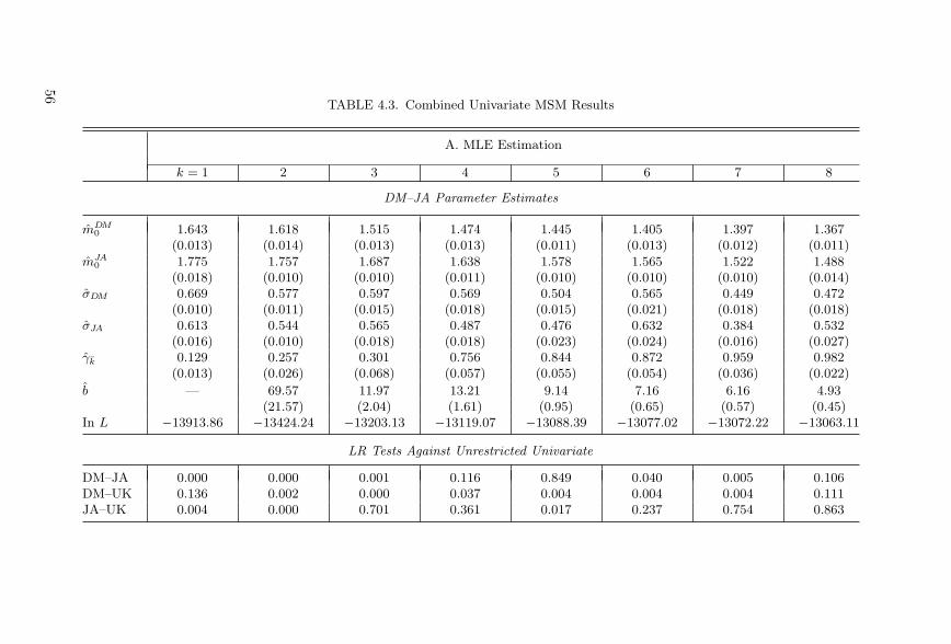
TABLE 4.3. Combined Univariate MSM Results

A. MLE Estimation

k = 1 2 3 4 5 6 7 8

DM–JA Parameter Estimates

mDM0 1.643 1.618 1.515 1.474 1.445 1.405 1.397 1.367

(0.013) (0.014) (0.013) (0.013) (0.011) (0.013) (0.012) (0.011)mJA

0 1.775 1.757 1.687 1.638 1.578 1.565 1.522 1.488(0.018) (0.010) (0.010) (0.011) (0.010) (0.010) (0.010) (0.014)

σDM 0.669 0.577 0.597 0.569 0.504 0.565 0.449 0.472(0.010) (0.011) (0.015) (0.018) (0.015) (0.021) (0.018) (0.018)

σJA 0.613 0.544 0.565 0.487 0.476 0.632 0.384 0.532(0.016) (0.010) (0.018) (0.018) (0.023) (0.024) (0.016) (0.027)

γk 0.129 0.257 0.301 0.756 0.844 0.872 0.959 0.982(0.013) (0.026) (0.068) (0.057) (0.055) (0.054) (0.036) (0.022)

b — 69.57 11.97 13.21 9.14 7.16 6.16 4.93(21.57) (2.04) (1.61) (0.95) (0.65) (0.57) (0.45)

In L −13913.86 −13424.24 −13203.13 −13119.07 −13088.39 −13077.02 −13072.22 −13063.11

LR Tests Against Unrestricted Univariate

DM–JA 0.000 0.000 0.001 0.116 0.849 0.040 0.005 0.106DM–UK 0.136 0.002 0.000 0.037 0.004 0.004 0.004 0.111JA–UK 0.004 0.000 0.701 0.361 0.017 0.237 0.754 0.863

56

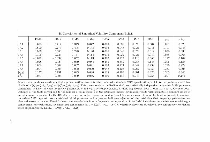
B. Correlation of Smoothed Volatility Component Beliefs

DM1 DM2 DM3 DM4 DM5 DM6 DM7 DM8 |rDM| r2DM

JA1 0.628 0.714 0.349 0.072 0.009 0.038 0.020 0.007 0.081 0.028JA2 0.690 0.774 0.405 0.135 0.016 0.048 0.027 0.011 0.101 0.043JA3 0.595 0.686 0.228 0.140 0.018 0.049 0.028 0.012 0.078 0.033JA4 0.306 0.234 0.147 0.114 0.036 0.022 0.027 0.013 0.065 0.065JA5 −0.019 −0.034 0.052 0.113 0.302 0.227 0.116 0.056 0.117 0.102JA6 0.028 0.023 0.040 0.084 0.255 0.352 0.258 0.145 0.206 0.186JA7 0.008 0.009 0.007 0.021 0.103 0.224 0.342 0.294 0.299 0.274JA8 0.004 0.004 0.002 0.009 0.048 0.123 0.287 0.353 0.333 0.304|rJA| 0.177 0.191 0.093 0.088 0.128 0.193 0.301 0.326 0.363 0.346r2JA 0.087 0.094 0.039 0.066 0.100 0.156 0.243 0.254 0.297 0.344

Notes: Panel A shows maximum likelihood estimation results for the combined univariate MSM specification, which for two series α and β haslikelihood L(rα

t ; mα0 , σα, b, γk)+L(rβ

t ; mβ0 , σβ , b, γk). This corresponds to the likelihood of two statistically independent univariate MSM processes

constrained to have the same frequency parameters b and γk. The sample consists of daily log returns from 1 June 1973 to 30 October 2003.Columns of the table correspond to the number of frequencies k in the estimated model. Estimation results with asymptotic standard errors inparentheses are presented for the DM-JA currency pair only. The second part of Panel A shows p-values from a likelihood ratio test of combinedunivariate MSM against two unrestricted MSM processes. A low p-value indicates rejection of the restriction that frequency parameters areidentical across currencies. Panel B then shows correlations from a frequency decomposition of the DM-JA combined univariate model with eightcomponents. For each series, the smoothed components Mk,t = E(Mk,t|r1, . . . , rT ) of volatility states are calculated. For convenience, we denotethese probabilities by DM1, . . . ,DM8, JA1, . . . ,JA8.

57

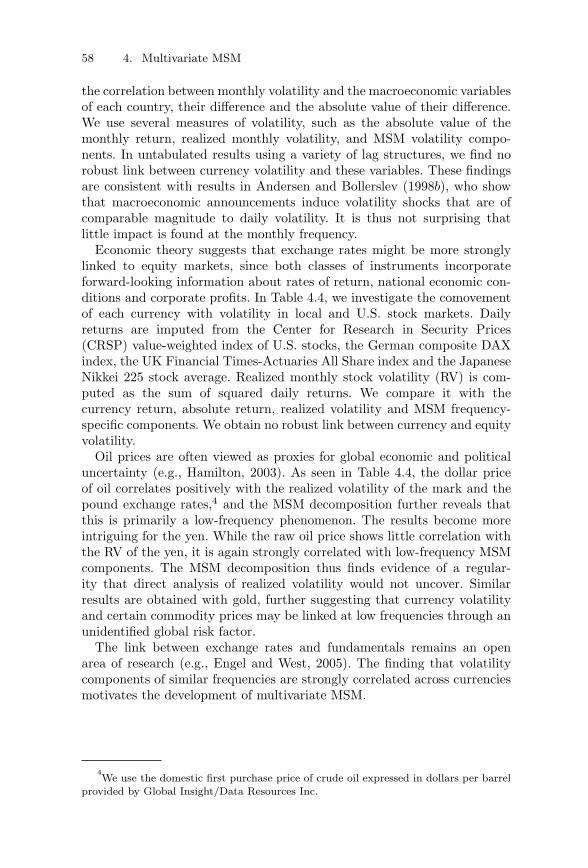
58 4. Multivariate MSM

the correlation between monthly volatility and the macroeconomic variablesof each country, their difference and the absolute value of their difference.We use several measures of volatility, such as the absolute value of themonthly return, realized monthly volatility, and MSM volatility compo-nents. In untabulated results using a variety of lag structures, we find norobust link between currency volatility and these variables. These findingsare consistent with results in Andersen and Bollerslev (1998b), who showthat macroeconomic announcements induce volatility shocks that are ofcomparable magnitude to daily volatility. It is thus not surprising thatlittle impact is found at the monthly frequency.

Economic theory suggests that exchange rates might be more stronglylinked to equity markets, since both classes of instruments incorporateforward-looking information about rates of return, national economic con-ditions and corporate profits. In Table 4.4, we investigate the comovementof each currency with volatility in local and U.S. stock markets. Dailyreturns are imputed from the Center for Research in Security Prices(CRSP) value-weighted index of U.S. stocks, the German composite DAXindex, the UK Financial Times-Actuaries All Share index and the JapaneseNikkei 225 stock average. Realized monthly stock volatility (RV) is com-puted as the sum of squared daily returns. We compare it with thecurrency return, absolute return, realized volatility and MSM frequency-specific components. We obtain no robust link between currency and equityvolatility.

Oil prices are often viewed as proxies for global economic and politicaluncertainty (e.g., Hamilton, 2003). As seen in Table 4.4, the dollar priceof oil correlates positively with the realized volatility of the mark and thepound exchange rates,4 and the MSM decomposition further reveals thatthis is primarily a low-frequency phenomenon. The results become moreintriguing for the yen. While the raw oil price shows little correlation withthe RV of the yen, it is again strongly correlated with low-frequency MSMcomponents. The MSM decomposition thus finds evidence of a regular-ity that direct analysis of realized volatility would not uncover. Similarresults are obtained with gold, further suggesting that currency volatilityand certain commodity prices may be linked at low frequencies through anunidentified global risk factor.

The link between exchange rates and fundamentals remains an openarea of research (e.g., Engel and West, 2005). The finding that volatilitycomponents of similar frequencies are strongly correlated across currenciesmotivates the development of multivariate MSM.

4We use the domestic first purchase price of crude oil expressed in dollars per barrel

provided by Global Insight/Data Resources Inc.

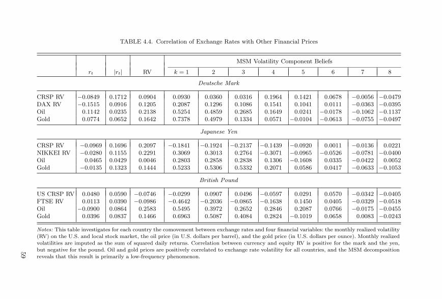
TABLE 4.4. Correlation of Exchange Rates with Other Financial Prices

MSM Volatility Component Beliefs

rt |rt| RV k = 1 2 3 4 5 6 7 8

Deutsche Mark

CRSP RV −0.0849 0.1712 0.0904 0.0930 0.0360 0.0316 0.1964 0.1421 0.0678 −0.0056 −0.0479DAX RV −0.1515 0.0916 0.1205 0.2087 0.1296 0.1086 0.1541 0.1041 0.0111 −0.0363 −0.0395Oil 0.1142 0.0235 0.2138 0.5254 0.4859 0.2685 0.1649 0.0241 −0.0178 −0.1062 −0.1137Gold 0.0774 0.0652 0.1642 0.7378 0.4979 0.1334 0.0571 −0.0104 −0.0613 −0.0755 −0.0497

Japanese Yen

CRSP RV −0.0969 0.1696 0.2097 −0.1841 −0.1924 −0.2137 −0.1439 −0.0920 0.0011 −0.0136 0.0221NIKKEI RV −0.0280 0.1155 0.2291 0.3069 0.3013 0.2764 −0.3071 −0.0965 −0.0526 −0.0781 −0.0400Oil 0.0465 0.0429 0.0046 0.2803 0.2858 0.2838 0.1306 −0.1608 0.0335 −0.0422 0.0052Gold −0.0135 0.1323 0.1444 0.5233 0.5306 0.5332 0.2071 0.0586 0.0417 −0.0633 −0.1053

British Pound

US CRSP RV 0.0480 0.0590 −0.0746 −0.0299 0.0907 0.0496 −0.0597 0.0291 0.0570 −0.0342 −0.0405FTSE RV 0.0113 0.0390 −0.0986 −0.4642 −0.2036 −0.0865 −0.1638 0.1450 0.0405 −0.0329 −0.0518Oil −0.0900 0.0864 0.2583 0.5495 0.3972 0.2652 0.2846 0.2087 0.0766 −0.0175 −0.0455Gold 0.0396 0.0837 0.1466 0.6963 0.5087 0.4084 0.2824 −0.1019 0.0658 0.0083 −0.0243

Notes: This table investigates for each country the comovement between exchange rates and four financial variables: the monthly realized volatility(RV) on the U.S. and local stock market, the oil price (in U.S. dollars per barrel), and the gold price (in U.S. dollars per ounce). Monthly realizedvolatilities are imputed as the sum of squared daily returns. Correlation between currency and equity RV is positive for the mark and the yen,but negative for the pound. Oil and gold prices are positively correlated to exchange rate volatility for all countries, and the MSM decompositionreveals that this result is primarily a low-frequency phenomenon.

59

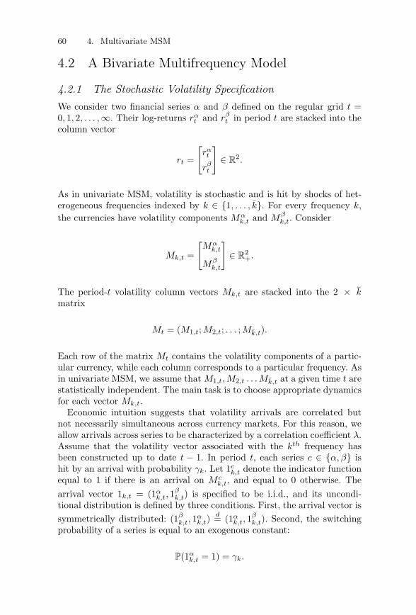
60 4. Multivariate MSM

4.2 A Bivariate Multifrequency Model

4.2.1 The Stochastic Volatility SpecificationWe consider two financial series α and β defined on the regular grid t =0, 1, 2, . . . ,∞. Their log-returns rα

t and rβt in period t are stacked into the

column vector

rt =

[rαt

rβt

]∈ R

2.

As in univariate MSM, volatility is stochastic and is hit by shocks of het-erogeneous frequencies indexed by k ∈ {1, . . . , k}. For every frequency k,the currencies have volatility components Mα

k,t and Mβk,t. Consider

Mk,t =

[Mα

k,t

Mβk,t

]∈ R

2+.

The period-t volatility column vectors Mk,t are stacked into the 2 × kmatrix

Mt = (M1,t;M2,t; . . . ;Mk,t).

Each row of the matrix Mt contains the volatility components of a partic-ular currency, while each column corresponds to a particular frequency. Asin univariate MSM, we assume that M1,t, M2,t . . . Mk,t at a given time t arestatistically independent. The main task is to choose appropriate dynamicsfor each vector Mk,t.

Economic intuition suggests that volatility arrivals are correlated butnot necessarily simultaneous across currency markets. For this reason, weallow arrivals across series to be characterized by a correlation coefficient λ.Assume that the volatility vector associated with the kth frequency hasbeen constructed up to date t − 1. In period t, each series c ∈ {α, β} ishit by an arrival with probability γk. Let 1c

k,t denote the indicator functionequal to 1 if there is an arrival on M c

k,t, and equal to 0 otherwise. Thearrival vector 1k,t = (1α

k,t, 1βk,t) is specified to be i.i.d., and its uncondi-

tional distribution is defined by three conditions. First, the arrival vector issymmetrically distributed: (1β

k,t, 1αk,t)

d= (1αk,t, 1

βk,t). Second, the switching

probability of a series is equal to an exogenous constant:

P(1αk,t = 1) = γk.

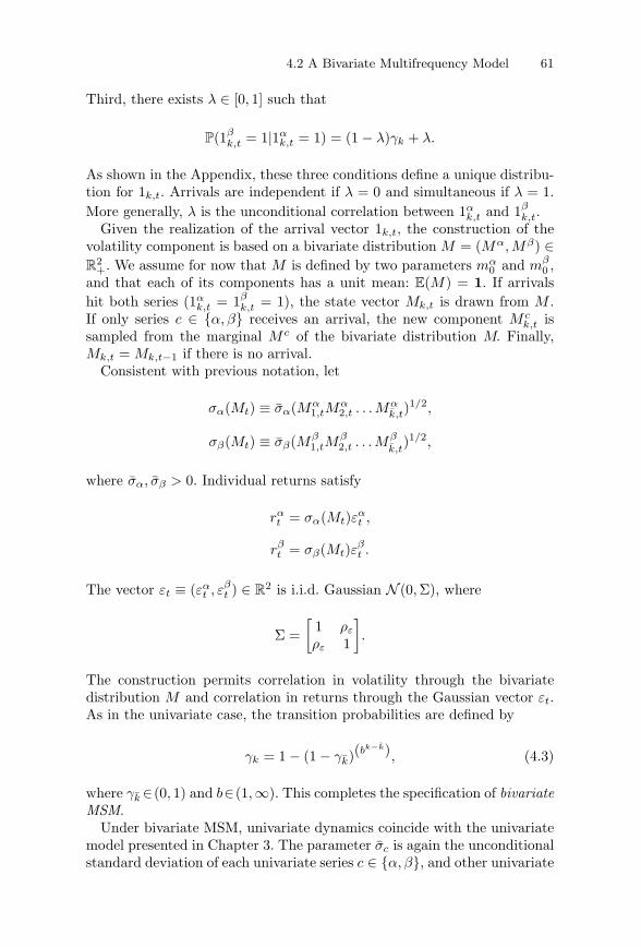
4.2 A Bivariate Multifrequency Model 61

Third, there exists λ ∈ [0, 1] such that

P(1βk,t = 1|1α

k,t = 1) = (1 − λ)γk + λ.

As shown in the Appendix, these three conditions define a unique distribu-tion for 1k,t. Arrivals are independent if λ = 0 and simultaneous if λ = 1.

More generally, λ is the unconditional correlation between 1αk,t and 1β

k,t.Given the realization of the arrival vector 1k,t, the construction of the

volatility component is based on a bivariate distribution M = (Mα, Mβ) ∈R

2+. We assume for now that M is defined by two parameters mα

0 and mβ0 ,

and that each of its components has a unit mean: E(M) = 1. If arrivalshit both series (1α

k,t = 1βk,t = 1), the state vector Mk,t is drawn from M .

If only series c ∈ {α, β} receives an arrival, the new component M ck,t is

sampled from the marginal M c of the bivariate distribution M. Finally,Mk,t = Mk,t−1 if there is no arrival.

Consistent with previous notation, let

σα(Mt) ≡ σα(Mα1,tM

α2,t . . . Mα

k,t)1/2,

σβ(Mt) ≡ σβ(Mβ1,tM

β2,t . . . Mβ

k,t)1/2,

where σα, σβ > 0. Individual returns satisfy

rαt = σα(Mt)εα

t ,

rβt = σβ(Mt)ε

βt .

The vector εt ≡ (εαt , εβ

t ) ∈ R2 is i.i.d. Gaussian N (0,Σ), where

Σ =[

1 ρε

ρε 1

].

The construction permits correlation in volatility through the bivariatedistribution M and correlation in returns through the Gaussian vector εt.As in the univariate case, the transition probabilities are defined by

γk = 1 − (1 − γk)(bk−k), (4.3)

where γk ∈(0, 1) and b∈(1,∞). This completes the specification of bivariateMSM.

Under bivariate MSM, univariate dynamics coincide with the univariatemodel presented in Chapter 3. The parameter σc is again the unconditionalstandard deviation of each univariate series c ∈ {α, β}, and other univariate

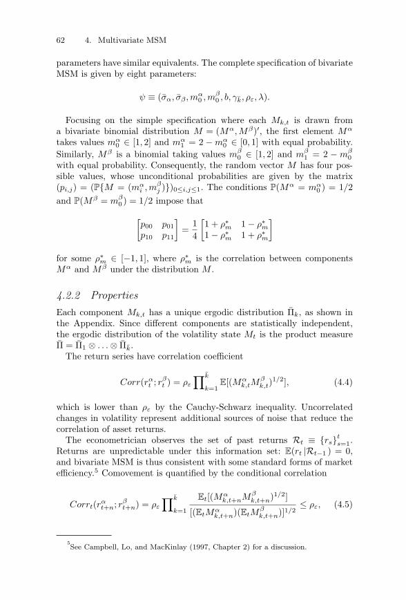
62 4. Multivariate MSM

parameters have similar equivalents. The complete specification of bivariateMSM is given by eight parameters:

ψ ≡ (σα, σβ , mα0 , mβ

0 , b, γk, ρε, λ).

Focusing on the simple specification where each Mk,t is drawn froma bivariate binomial distribution M = (Mα, Mβ)′, the first element Mα

takes values mα0 ∈ [1, 2] and mα

1 = 2 − mα0 ∈ [0, 1] with equal probability.

Similarly, Mβ is a binomial taking values mβ0 ∈ [1, 2] and mβ

1 = 2 − mβ0

with equal probability. Consequently, the random vector M has four pos-sible values, whose unconditional probabilities are given by the matrix(pi,j) = (P{M = (mα

i , mβj )})0≤i,j≤1. The conditions P(Mα = mα

0 ) = 1/2and P(Mβ = mβ

0 ) = 1/2 impose that

[p00 p01p10 p11

]=

14

[1 + ρ∗

m 1 − ρ∗m

1 − ρ∗m 1 + ρ∗

m

]

for some ρ∗m ∈ [−1, 1], where ρ∗

m is the correlation between componentsMα and Mβ under the distribution M .

4.2.2 PropertiesEach component Mk,t has a unique ergodic distribution Πk, as shown inthe Appendix. Since different components are statistically independent,the ergodic distribution of the volatility state Mt is the product measureΠ = Π1 ⊗ . . . ⊗ Πk.

The return series have correlation coefficient

Corr(rαt ; rβ

t ) = ρε

∏k

k=1E[(Mα

k,tMβk,t)

1/2], (4.4)

which is lower than ρε by the Cauchy-Schwarz inequality. Uncorrelatedchanges in volatility represent additional sources of noise that reduce thecorrelation of asset returns.

The econometrician observes the set of past returns Rt ≡ {rs}ts=1.

Returns are unpredictable under this information set: E(rt |Rt−1 ) = 0,and bivariate MSM is thus consistent with some standard forms of marketefficiency.5 Comovement is quantified by the conditional correlation

Corrt(rαt+n; rβ

t+n) = ρε

∏k

k=1

Et[(Mαk,t+nMβ

k,t+n)1/2]

[(EtMαk,t+n)(EtM

βk,t+n)]1/2

≤ ρε, (4.5)

5See Campbell, Lo, and MacKinlay (1997, Chapter 2) for a discussion.

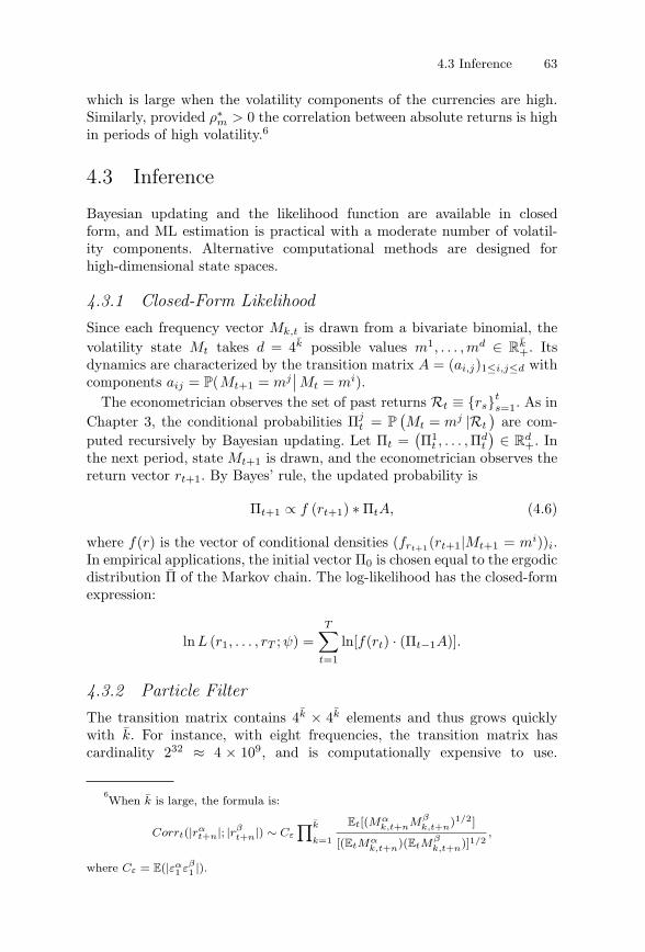
4.3 Inference 63

which is large when the volatility components of the currencies are high.Similarly, provided ρ∗

m > 0 the correlation between absolute returns is highin periods of high volatility.6

4.3 Inference

Bayesian updating and the likelihood function are available in closedform, and ML estimation is practical with a moderate number of volatil-ity components. Alternative computational methods are designed forhigh-dimensional state spaces.

4.3.1 Closed-Form LikelihoodSince each frequency vector Mk,t is drawn from a bivariate binomial, thevolatility state Mt takes d = 4k possible values m1, . . . , md ∈ R

k+. Its

dynamics are characterized by the transition matrix A = (ai,j)1≤i,j≤d withcomponents aij = P(Mt+1 = mj

∣∣ Mt = mi).The econometrician observes the set of past returns Rt ≡ {rs}t

s=1. As inChapter 3, the conditional probabilities Πj

t = P(Mt = mj |Rt

)are com-

puted recursively by Bayesian updating. Let Πt =(Π1

t , . . . ,Πdt

)∈ R

d+. In

the next period, state Mt+1 is drawn, and the econometrician observes thereturn vector rt+1. By Bayes’ rule, the updated probability is

Πt+1 ∝ f (rt+1) ∗ ΠtA, (4.6)

where f(r) is the vector of conditional densities (frt+1(rt+1|Mt+1 = mi))i.In empirical applications, the initial vector Π0 is chosen equal to the ergodicdistribution Π of the Markov chain. The log-likelihood has the closed-formexpression:

lnL (r1, . . . , rT ;ψ) =T∑

t=1

ln[f(rt) · (Πt−1A)].

4.3.2 Particle FilterThe transition matrix contains 4k × 4k elements and thus grows quicklywith k. For instance, with eight frequencies, the transition matrix hascardinality 232 ≈ 4 × 109, and is computationally expensive to use.

6When k is large, the formula is:

Corrt(|rαt+n|; |rβ

t+n|) ∼ Cε

∏k

k=1

Et[(Mαk,t+nMβ

k,t+n)1/2]

[(EtMαk,t+n)(EtM

βk,t+n)]1/2

,

where Cε = E(|εα1 εβ

1 |).

64 4. Multivariate MSM

Following the literature on Markov chains,7 we now propose a simulation-based inference methodology based on a particle filter, a recursive algorithmthat generates independent draws

M(1)t , . . . , M

(B)t

from the conditional distribution Πt.We begin at t = 0 by drawing B states from the ergodic distribution

Π. For any t ≥ 0, assume that M(1)t , . . . , M

(B)t have been independently

sampled from Πt. Given a new return rt+1, we rewrite the updating formula(4.6) as

Πjt+1 ∝ frt+1

(rt+1|Mt+1 = mj

) d∑

i=1

P(Mt+1 = mj |Mt = mi

)Πi

t.

We obtain M(1)t+1, . . . , M

(B)t+1 by simulating each M

(b)t one-step forward and

reweighting using an importance sampler. Specifically:

1. Simulate the Markov chain one-step ahead to obtain M(1)t+1 given

M(1)t . Repeat B times to generate B draws M

(1)t+1, . . . , M

(B)t+1 . This prelim-

inary step only uses information available at date t and must therefore beadjusted to account for the new return.

2. Draw a random number q from 1 to B with probability

P(q = b) ≡frt+1(rt+1|Mt+1 = M

(b)t+1)∑B

b′=1 frt+1(rt+1|Mt+1 = M(b′)t+1)

.

The vector M(1)t+1 = M

(q)t+1 is a draw from Πt+1. Repeat B times to obtain

B draws M(1)t+1, . . . , M

(B)t+1 .

This recursive procedure provides a discrete approximation to Bayesianupdating, which is computationally convenient in large state spaces.

4.3.3 Simulated LikelihoodWe can use the particle filter to compute the likelihood function.Each one-step ahead density satisfies f(rt|Rt−1) =

∑di=1 f(rt|Mt = mi)

7See, for instance, Chib, Nardari, and Shephard (2002), Jacquier, Polson, and Rossi

(1994), and Pitt and Shephard (1999).

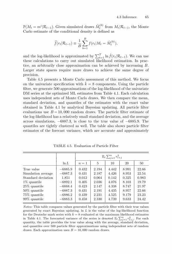
4.3 Inference 65

P(Mt = mi|Rt−1). Given simulated draws M(b)t from Mt|Rt−1, the Monte

Carlo estimate of the conditional density is defined as

f(rt|Rt−1) ≡ 1B

B∑

b=1

f(rt|Mt = M(b)t ),

and the log-likelihood is approximated by∑T

t=1 ln f(rt|Rt−1). We can usethese calculations to carry out simulated likelihood estimation. In prac-tice, an arbitrarily close approximation can be achieved by increasing B.Larger state spaces require more draws to achieve the same degree ofprecision.

Table 4.5 presents a Monte Carlo assessment of this method. We focuson the univariate specification with k = 8 components. Using the particlefilter, we generate 500 approximations of the log-likelihood of the univariateDM series at the optimized ML estimates from Table 4.1. Each calculationuses independent sets of Monte Carlo draws. We then compare the mean,standard deviation, and quantiles of the estimates with the exact valueobtained in Table 4.1 by analytical Bayesian updating. All particle filterevaluations use B = 10, 000 random draws. The particle filter estimate ofthe log-likelihood has a relatively small standard deviation, and the averageacross simulations, −6887.3, is close to the true value of −6885.9. Thequantiles are tightly clustered as well. The table also shows particle filterestimates of the forecast variance, which are accurate and approximately

TABLE 4.5. Evaluation of Particle Filter

Et

∑nj=1 r2

t+j

ln L n = 1 5 10 20 50

True value −6885.9 0.432 2.194 4.442 8.991 22.66Simulation average −6887.3 0.431 2.187 4.426 8.953 22.54Standard deviation 1.851 0.012 0.064 0.142 0.325 0.9831% quantile −6892.1 0.405 2.036 4.076 8.103 19.7925% quantile −6888.4 0.423 2.147 4.338 8.747 21.9750% quantile −6887.3 0.431 2.191 4.435 8.957 22.6675% quantile −6886.2 0.439 2.231 4.525 9.179 23.2399% quantile −6883.3 0.458 2.330 4.739 9.633 24.42

Notes: This table compares values generated by the particle filter with their true valuesgenerated by exact Bayesian updating. ln L is the value of the log-likelihood functionfor the Deutsche mark series with k = 8 evaluated at the maximum likelihood estimatesin Table 4.1. The forecasted variance of the series is denoted Et

∑nj=1 r2

t+j . For eachquantity, the table provides the true value along with the average, standard deviation,and quantiles over 500 particle filter approximations using independent sets of randomdraws. Each approximation uses B = 10, 000 random draws.

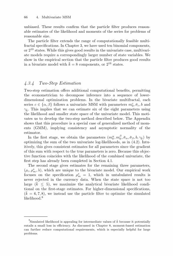
66 4. Multivariate MSM

unbiased. These results confirm that the particle filter produces reason-able estimates of the likelihood and moments of the series for problems ofreasonable size.

The particle filter extends the range of computationally feasible multi-fractal specifications. In Chapter 3, we have used ten binomial components,or 210 states. While this gives good results in the univariate case, multivari-ate models require a correspondingly larger number of state variables. Weshow in the empirical section that the particle filter produces good resultsin a bivariate model with k = 8 components, or 216 states.

4.3.4 Two-Step EstimationTwo-step estimation offers additional computational benefits, permittingthe econometrician to decompose inference into a sequence of lower-dimensional optimization problems. In the bivariate multifractal, eachseries c ∈ {α, β} follows a univariate MSM with parameters mc

0, σc, b andγk. This implies that we can estimate six of the eight parameters usingthe likelihood and smaller state space of the univariate model. This moti-vates us to develop the two-step method described below. The Appendixshows that this procedure is a special case of generalized method of mom-ents (GMM), implying consistency and asymptotic normality of theestimator.

In the first stage, we obtain the parameters (mα0 , mβ

0 , σα, σβ , b, γk) byoptimizing the sum of the two univariate log-likelihoods, as in (4.2). Intu-itively, this gives consistent estimates for all parameters since the gradientof this sum with respect to the true parameters is zero. Because this objec-tive function coincides with the likelihood of the combined univariate, thefirst step has already been completed in Section 4.1.

The second stage gives estimates for the remaining three parameters,(ρε, ρ

∗m, λ), which are unique to the bivariate model. Our empirical work

focuses on the specification ρ∗m = 1, which in untabulated results is

never rejected in the currency data. When the state space is not toolarge (k ≤ 5), we maximize the analytical bivariate likelihood condi-tional on the first-stage estimates. For higher-dimensional specifications,(k = 6, 7, 8), we instead use the particle filter to optimize the simulatedlikelihood.8

8Simulated likelihood is appealing for intermediate values of k because it potentially

entails a small loss in efficiency. As discussed in Chapter 8, moment-based estimationcan further reduce computational requirements, which is especially helpful for largeproblems.

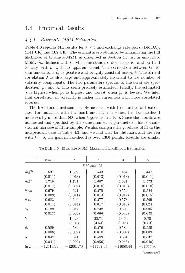
4.4 Empirical Results 67

4.4 Empirical Results

4.4.1 Bivariate MSM EstimatesTable 4.6 reports ML results for k ≤ 5 and exchange rate pairs (DM,JA),(DM,UK) and (JA,UK). The estimates are obtained by maximizing the fulllikelihood of bivariate MSM, as described in Section 4.3. As in univariateMSM, m0 declines with k, while the standard deviations σα and σβ tendto vary with k, with no apparent trend. The correlation between Gaus-sian innovations ρε is positive and roughly constant across k. The arrivalcorrelation λ is also large and approximately invariant to the number ofvolatility components. The two parameters specific to the bivariate spec-ification, ρε and λ, thus seem precisely estimated. Finally, the estimatedλ is highest when ρε is highest and lowest when ρε is lowest. We inferthat correlation in volatility is higher for currencies with more correlatedreturns.

The likelihood functions sharply increase with the number of frequen-cies. For instance, with the mark and the yen series, the log-likelihoodincreases by more than 800 when k goes from 1 to 5. Since the models arenonnested and specified by the same number of parameters, this is a sub-stantial increase of fit in-sample. We also compare the goodness of fit to theindependent case in Table 4.3, and we find that for the mark and the yenwith k = 5, the gain in likelihood is over 1300 points. Results are similar

TABLE 4.6. Bivariate MSM: Maximum Likelihood Estimation

k = 1 2 3 4 5

DM and JA

mDM0 1.637 1.589 1.543 1.484 1.447

(0.011) (0.013) (0.013) (0.013) (0.011)mJA

0 1.718 1.701 1.667 1.621 1.573(0.011) (0.009) (0.010) (0.010) (0.010)

σDM 0.679 0.621 0.575 0.559 0.524(0.009) (0.011) (0.014) (0.017) (0.015)

σJA 0.683 0.649 0.577 0.573 0.509(0.011) (0.014) (0.017) (0.018) (0.024)

γk 0.122 0.217 0.732 0.828 0.905(0.013) (0.022) (0.066) (0.049) (0.038)

b — 16.23 23.71 13.60 8.70(3.09) (4.54) (1.48) (0.83)

ρε 0.580 0.589 0.576 0.580 0.580(0.008) (0.009) (0.010) (0.009) (0.009)

λ 0.647 0.641 0.589 0.634 0.637(0.041) (0.039) (0.056) (0.048) (0.049)

ln L −12519.99 −12001.70 −11797.05 −11688.44 −11655.80

(continued)

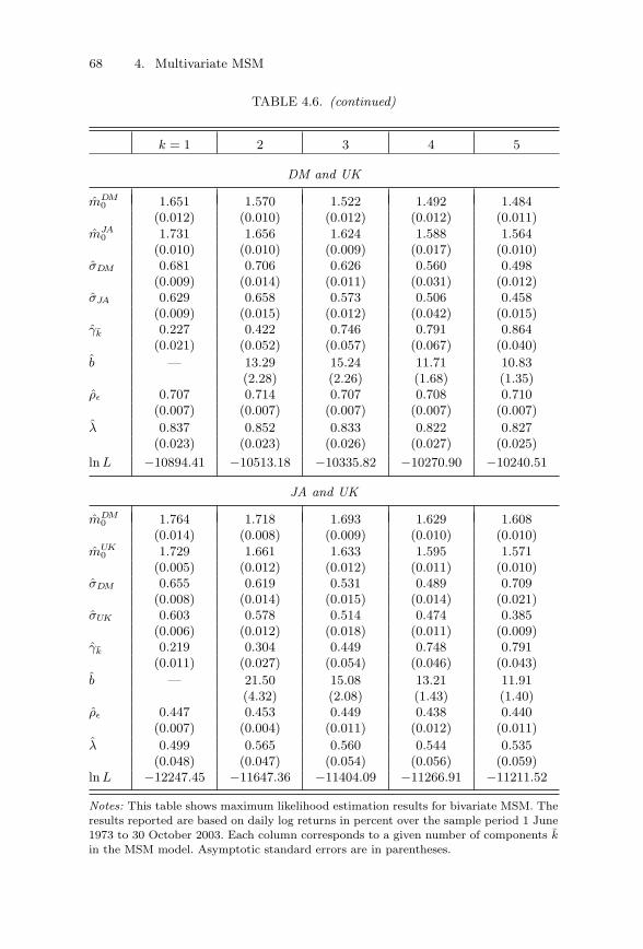
68 4. Multivariate MSM

TABLE 4.6. (continued)

k = 1 2 3 4 5

DM and UK

mDM0 1.651 1.570 1.522 1.492 1.484

(0.012) (0.010) (0.012) (0.012) (0.011)mJA

0 1.731 1.656 1.624 1.588 1.564(0.010) (0.010) (0.009) (0.017) (0.010)

σDM 0.681 0.706 0.626 0.560 0.498(0.009) (0.014) (0.011) (0.031) (0.012)

σJA 0.629 0.658 0.573 0.506 0.458(0.009) (0.015) (0.012) (0.042) (0.015)

γk 0.227 0.422 0.746 0.791 0.864(0.021) (0.052) (0.057) (0.067) (0.040)

b — 13.29 15.24 11.71 10.83(2.28) (2.26) (1.68) (1.35)

ρε 0.707 0.714 0.707 0.708 0.710(0.007) (0.007) (0.007) (0.007) (0.007)

λ 0.837 0.852 0.833 0.822 0.827(0.023) (0.023) (0.026) (0.027) (0.025)

ln L −10894.41 −10513.18 −10335.82 −10270.90 −10240.51

JA and UK

mDM0 1.764 1.718 1.693 1.629 1.608

(0.014) (0.008) (0.009) (0.010) (0.010)mUK

0 1.729 1.661 1.633 1.595 1.571(0.005) (0.012) (0.012) (0.011) (0.010)

σDM 0.655 0.619 0.531 0.489 0.709(0.008) (0.014) (0.015) (0.014) (0.021)

σUK 0.603 0.578 0.514 0.474 0.385(0.006) (0.012) (0.018) (0.011) (0.009)

γk 0.219 0.304 0.449 0.748 0.791(0.011) (0.027) (0.054) (0.046) (0.043)

b — 21.50 15.08 13.21 11.91(4.32) (2.08) (1.43) (1.40)

ρε 0.447 0.453 0.449 0.438 0.440(0.007) (0.004) (0.011) (0.012) (0.011)

λ 0.499 0.565 0.560 0.544 0.535(0.048) (0.047) (0.054) (0.056) (0.059)

ln L −12247.45 −11647.36 −11404.09 −11266.91 −11211.52

Notes: This table shows maximum likelihood estimation results for bivariate MSM. Theresults reported are based on daily log returns in percent over the sample period 1 June1973 to 30 October 2003. Each column corresponds to a given number of components kin the MSM model. Asymptotic standard errors are in parentheses.

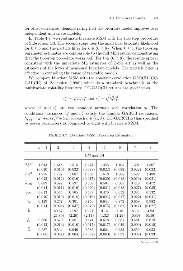
4.4 Empirical Results 69

for other currencies, demonstrating that the bivariate model improves overindependent univariate models.

In Table 4.7, we reestimate bivariate MSM with the two-step procedureof Subsection 4.3. The second stage uses the analytical bivariate likelihoodfor k ≤ 5 and the particle filter for k ∈ {6, 7, 8}. When k ≤ 5, the two-stepparameter estimates are comparable to the full ML results, demonstratingthat the two-step procedure works well. For k ∈ {6, 7, 8}, the results appearconsistent with the univariate ML estimates of Table 4.1 as well as theestimates of the lower dimensional bivariate models. The particle filter iseffective in extending the range of tractable models.

We compare bivariate MSM with the constant correlation GARCH (CC-GARCH) of Bollerslev (1990), which is a standard benchmark in themultivariate volatility literature. CC-GARCH returns are specified as

rαt =

√hα

t εαt and rβ

t =√

hβt εβ

t ,

where εαt and εβ

t are two standard normals with correlation ρε. Theconditional variances hα

t and hβt satisfy the familiar GARCH recursions:

hct+1 = ωc+ac(εc

t)2+bch

ct for each c ∈ {α, β}. CC-GARCH is thus specified

by seven parameters as compared to eight with bivariate MSM.

TABLE 4.7. Bivariate MSM: Two-Step Estimation

k = 1 2 3 4 5 6 7 8

DM and JA

mDM0 1.643 1.618 1.515 1.474 1.445 1.405 1.397 1.367

(0.020) (0.019) (0.022) (0.023) (0.022) (0.022) (0.022) (0.022)mJA

0 1.775 1.757 1.687 1.638 1.578 1.565 1.522 1.488(0.013) (0.012) (0.016) (0.017) (0.020) (0.018) (0.019) (0.021)

σDM 0.669 0.577 0.597 0.569 0.504 0.565 0.449 0.472(0.014) (0.011) (0.019) (0.020) (0.021) (0.018) (0.027) (0.035)

σJA 0.613 0.544 0.565 0.487 0.476 0.632 0.384 0.532(0.010) (0.010) (0.018) (0.016) (0.021) (0.017) (0.022) (0.041)

γk 0.129 0.257 0.301 0.756 0.844 0.872 0.959 0.982(0.014) (0.024) (0.037) (0.072) (0.075) (0.081) (0.047) (0.027)

b — 69.57 11.97 13.21 9.14 7.16 6.16 4.93(21.80) (2.20) (2.11) (1.32) (1.29) (0.86) (0.56)

ρε 0.566 0.570 0.581 0.574 0.578 0.581 0.581 0.618(0.013) (0.014) (0.016) (0.017) (0.017) (0.049) (0.009) (0.010)

λ 0.587 0.544 0.646 0.585 0.624 0.633 0.659 0.633(0.065) (0.067) (0.064) (0.082) (0.080) (0.032) (0.038) (0.023)

(continued)

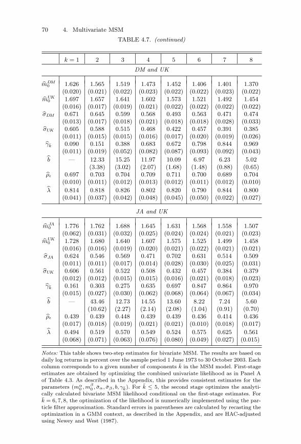
70 4. Multivariate MSM

TABLE 4.7. (continued)

k = 1 2 3 4 5 6 7 8

DM and UK

mDM0 1.626 1.565 1.519 1.473 1.452 1.406 1.401 1.370

(0.020) (0.021) (0.022) (0.023) (0.022) (0.022) (0.023) (0.022)mUK

0 1.697 1.657 1.641 1.602 1.573 1.521 1.492 1.454(0.016) (0.017) (0.019) (0.021) (0.022) (0.022) (0.022) (0.022)

σDM 0.671 0.645 0.599 0.568 0.493 0.563 0.471 0.474(0.013) (0.017) (0.018) (0.021) (0.018) (0.018) (0.028) (0.033)

σUK 0.605 0.588 0.515 0.468 0.422 0.457 0.391 0.385(0.011) (0.015) (0.015) (0.016) (0.017) (0.020) (0.019) (0.026)

γk 0.090 0.151 0.388 0.683 0.672 0.798 0.844 0.969(0.011) (0.019) (0.052) (0.082) (0.087) (0.093) (0.092) (0.043)

b — 12.33 15.25 11.97 10.09 6.97 6.23 5.02(3.38) (3.02) (2.07) (1.68) (1.48) (0.88) (0.65)

ρε 0.697 0.703 0.704 0.709 0.711 0.700 0.689 0.704(0.010) (0.011) (0.012) (0.013) (0.012) (0.011) (0.012) (0.010)

λ 0.814 0.818 0.826 0.802 0.820 0.790 0.844 0.800(0.041) (0.037) (0.042) (0.048) (0.045) (0.050) (0.022) (0.027)

JA and UK

mJA0 1.776 1.762 1.688 1.645 1.631 1.568 1.558 1.507

(0.062) (0.031) (0.032) (0.025) (0.024) (0.024) (0.021) (0.023)mUK

0 1.728 1.680 1.640 1.607 1.575 1.525 1.499 1.458(0.016) (0.016) (0.019) (0.020) (0.021) (0.022) (0.021) (0.021)

σJA 0.624 0.546 0.569 0.471 0.702 0.631 0.514 0.509(0.011) (0.011) (0.017) (0.014) (0.028) (0.030) (0.025) (0.031)

σUK 0.606 0.561 0.522 0.508 0.432 0.457 0.384 0.379(0.012) (0.012) (0.015) (0.015) (0.016) (0.021) (0.018) (0.023)

γk 0.161 0.303 0.275 0.635 0.697 0.847 0.864 0.970(0.015) (0.027) (0.030) (0.062) (0.068) (0.064) (0.067) (0.034)

b — 43.46 12.73 14.55 13.60 8.22 7.24 5.60(10.62) (2.27) (2.14) (2.08) (1.04) (0.91) (0.70)

ρε 0.439 0.439 0.448 0.439 0.439 0.436 0.414 0.436(0.017) (0.018) (0.019) (0.021) (0.021) (0.010) (0.018) (0.017)

λ 0.494 0.519 0.570 0.549 0.524 0.575 0.625 0.561(0.068) (0.071) (0.063) (0.076) (0.080) (0.049) (0.027) (0.015)

Notes: This table shows two-step estimates for bivariate MSM. The results are based ondaily log returns in percent over the sample period 1 June 1973 to 30 October 2003. Eachcolumn corresponds to a given number of components k in the MSM model. First-stageestimates are obtained by optimizing the combined univariate likelihood as in Panel Aof Table 4.3. As described in the Appendix, this provides consistent estimates for theparameters (mα

0 , mβ0 , σα, σβ , b, γk). For k ≤ 5, the second stage optimizes the analyti-

cally calculated bivariate MSM likelihood conditional on the first-stage estimates. Fork = 6, 7, 8, the optimization of the likelihood is numerically implemented using the par-ticle filter approximation. Standard errors in parentheses are calculated by recasting theoptimization in a GMM context, as described in the Appendix, and are HAC-adjustedusing Newey and West (1987).

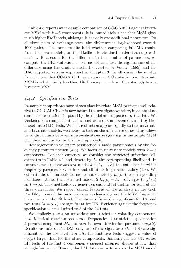
4.4 Empirical Results 71

Table 4.8 reports an in-sample comparison of CC-GARCH against bivari-ate MSM with k = 5 components. It is immediately clear that MSM givesmuch higher likelihoods, although it has only one additional parameter. Forall three pairs of exchange rates, the difference in log-likelihood exceeds1000 points. The same results hold whether comparing full ML resultsfrom the two models, or the likelihoods obtained under two-step esti-mation. To account for the difference in the number of parameters, wecompute the BIC statistic for each model, and test the significance of thedifference using the original method suggested by Vuong (1989) and theHAC-adjusted version explained in Chapter 3. In all cases, the p-valuefrom the test that CC-GARCH has a superior BIC statistic to multivariateMSM is substantially less than 1%. In-sample evidence thus strongly favorsbivariate MSM.

4.4.2 Specification TestsIn-sample comparisons have shown that bivariate MSM performs well rela-tive to CC-GARCH. It is now natural to investigate whether, in an absolutesense, the restrictions imposed by the model are supported by the data. Weweaken one assumption at a time, and we assess improvement in fit by like-lihood ratio (LR) tests. When a restriction applies equally to the univariateand bivariate models, we choose to test on the univariate series. This allowsus to distinguish between misspecifications originating in univariate MSMand those unique to the bivariate approach.

Heterogeneity in volatility persistence is made parsimonious by the fre-quency parameterization (4.3). We focus on univariate models with k = 8components. For each currency, we consider the restricted univariate MLestimates in Table 4.1 and denote by Lr the corresponding likelihood. Incontrast, we call unrestricted model k ∈ {1, . . . , k} the extension in whichfrequency parameter γk is free and all other frequencies satisfy (4.3). Weestimate the kth unrestricted model and denote by Lu(k) the correspondinglikelihood. Under the restricted model, 2[Lu(k) − Lr] converges to χ2 (1)as T → ∞. This methodology generates eight LR statistics for each of thethree currencies. We report salient features of the analysis in the text.For DM, none of the tests provides evidence against the MSM frequencyrestrictions at the 1% level. One statistic (k = 6) is significant for JA, andtwo tests (k = 6, 7) are significant for UK. Evidence against the frequencyspecification is thus limited to 3 of the 24 tests.

We similarly assess on univariate series whether volatility componentshave identical distributions across frequencies. Unrestricted specificationk permits component Mk,t to have its own distribution parameter m0(k).Results are mixed. For DM, only two of the eight tests (k = 1, 6) are sig-nificant at the 1% level. For JA, the first five tests suggest a value ofm0(k) larger than for the other components. Similarly for the UK series,LR tests of the first 4 components suggest stronger shocks at low thanat high-frequency. Overall, the DM data seems to match the MSM model

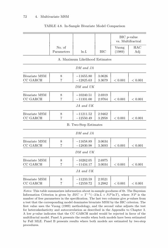
72 4. Multivariate MSM

TABLE 4.8. In-Sample Bivariate Model Comparison

BIC p-valuevs. Multifractral

No. of Vuong HACParameters ln L BIC (1989) Adj

A. Maximum Likelihood Estimates

DM and JA

Bivariate MSM 8 −11655.80 3.0626CC GARCH 7 −12825.63 3.3679 < 0.001 < 0.001

DM and UK

Bivariate MSM 8 −10240.51 2.6919CC GARCH 7 −11331.00 2.9764 < 0.001 < 0.001

JA and UK

Bivariate MSM 8 −11211.52 2.9462CC GARCH 7 −12550.49 3.2958 < 0.001 < 0.001

B. Two-Step Estimates

DM and JA

Bivariate MSM 8 −11658.89 3.0634CC GARCH 7 −12830.98 3.3693 < 0.001 < 0.001

DM and UK

Bivariate MSM 8 −10262.05 2.6975CC GARCH 7 −11434.17 3.0034 < 0.001 < 0.001

JA and UK

Bivariate MSM 8 −11233.59 2.9521CC GARCH 7 −12559.72 3.2982 < 0.001 < 0.001

Notes: This table summarizes information about in-sample goodness of fit. The BayesianInformation Criterion is given by BIC = T −1(−2 ln L + NP ln T ), where NP is thenumber of free parameters in the specification. The last two columns give p-values froma test that the corresponding model dominates bivariate MSM by the BIC criterion. Thefirst value uses the Vuong (1989) methodology, and the second value adjusts the testfor heteroskedasticity and autocorrelation as described in the Appendix to Chapter 3.A low p-value indicates that the CC GARCH model would be rejected in favor of themultifractal model. Panel A presents the results when both models have been estimatedby Full MLE. Panel B presents results where both models are estimated by two-stepprocedures.

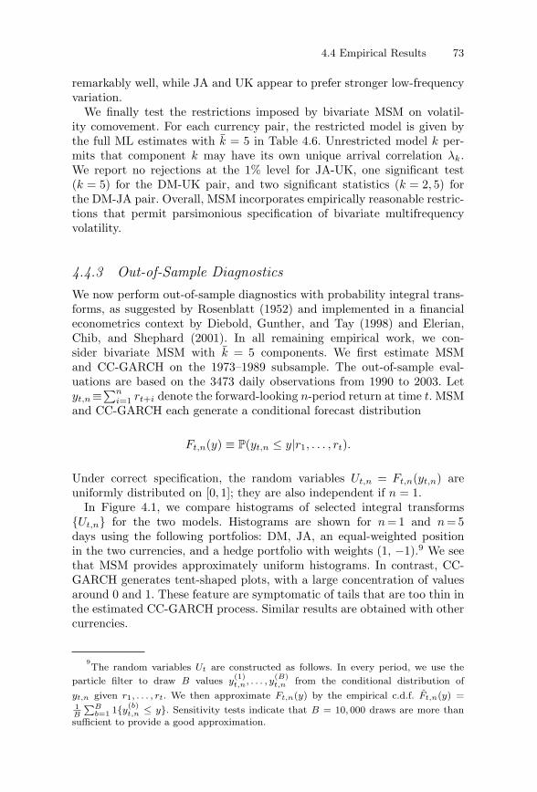
4.4 Empirical Results 73

remarkably well, while JA and UK appear to prefer stronger low-frequencyvariation.

We finally test the restrictions imposed by bivariate MSM on volatil-ity comovement. For each currency pair, the restricted model is given bythe full ML estimates with k = 5 in Table 4.6. Unrestricted model k per-mits that component k may have its own unique arrival correlation λk.We report no rejections at the 1% level for JA-UK, one significant test(k = 5) for the DM-UK pair, and two significant statistics (k = 2, 5) forthe DM-JA pair. Overall, MSM incorporates empirically reasonable restric-tions that permit parsimonious specification of bivariate multifrequencyvolatility.

4.4.3 Out-of-Sample DiagnosticsWe now perform out-of-sample diagnostics with probability integral trans-forms, as suggested by Rosenblatt (1952) and implemented in a financialeconometrics context by Diebold, Gunther, and Tay (1998) and Elerian,Chib, and Shephard (2001). In all remaining empirical work, we con-sider bivariate MSM with k = 5 components. We first estimate MSMand CC-GARCH on the 1973–1989 subsample. The out-of-sample eval-uations are based on the 3473 daily observations from 1990 to 2003. Letyt,n ≡

∑ni=1 rt+i denote the forward-looking n-period return at time t. MSM

and CC-GARCH each generate a conditional forecast distribution

Ft,n(y) ≡ P(yt,n ≤ y|r1, . . . , rt).

Under correct specification, the random variables Ut,n = Ft,n(yt,n) areuniformly distributed on [0, 1]; they are also independent if n = 1.

In Figure 4.1, we compare histograms of selected integral transforms{Ut,n} for the two models. Histograms are shown for n = 1 and n = 5days using the following portfolios: DM, JA, an equal-weighted positionin the two currencies, and a hedge portfolio with weights (1, −1).9 We seethat MSM provides approximately uniform histograms. In contrast, CC-GARCH generates tent-shaped plots, with a large concentration of valuesaround 0 and 1. These feature are symptomatic of tails that are too thin inthe estimated CC-GARCH process. Similar results are obtained with othercurrencies.

9The random variables Ut are constructed as follows. In every period, we use the

particle filter to draw B values y(1)t,n, . . . , y

(B)t,n from the conditional distribution of

yt,n given r1, . . . , rt. We then approximate Ft,n(y) by the empirical c.d.f. Ft,n(y) =1B

∑Bb=1 1{y

(b)t,n ≤ y}. Sensitivity tests indicate that B = 10, 000 draws are more than

sufficient to provide a good approximation.

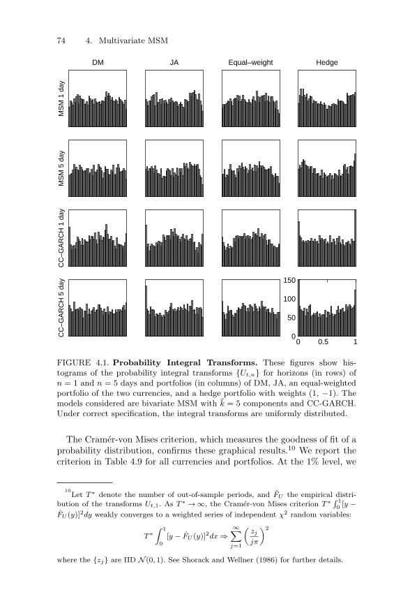
74 4. Multivariate MSM

DMM

SM

1 d

ayJA Equal–weight Hedge

MS

M 5

day

CC

–GA

RC

H 1

day

CC

–GA

RC

H 5

day

0 0.5 10

50

100

150

FIGURE 4.1. Probability Integral Transforms. These figures show his-tograms of the probability integral transforms {Ut,n} for horizons (in rows) ofn = 1 and n = 5 days and portfolios (in columns) of DM, JA, an equal-weightedportfolio of the two currencies, and a hedge portfolio with weights (1, −1). Themodels considered are bivariate MSM with k = 5 components and CC-GARCH.Under correct specification, the integral transforms are uniformly distributed.

The Cramer-von Mises criterion, which measures the goodness of fit of aprobability distribution, confirms these graphical results.10 We report thecriterion in Table 4.9 for all currencies and portfolios. At the 1% level, we

10Let T ∗ denote the number of out-of-sample periods, and FU the empirical distri-

bution of the transforms Ut,1. As T ∗ → ∞, the Cramer-von Mises criterion T ∗ ∫ 10 [y −

FU (y)]2dy weakly converges to a weighted series of independent χ2 random variables:

T ∗∫ 1

0[y − FU (y)]2dx ⇒

∞∑j=1

(zj

jπ

)2

where the {zj} are IID N (0, 1). See Shorack and Wellner (1986) for further details.

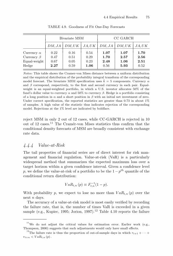
4.4 Empirical Results 75

TABLE 4.9. Goodness of Fit One-Day Forecasts

Bivariate MSM CC GARCH

DM, JA DM, UK JA, UK DM, JA DM, UK JA, UK

Currency α 0.22 0.16 0.54 1.07 1.07 1.70Currency β 0.47 0.51 0.29 1.70 2.57 2.56Equal-weight 0.67 0.05 0.23 2.48 1.06 2.51Hedge 2.27 0.59 1.06 0.56 5.93 0.52

Notes: This table shows the Cramer-von Mises distance between a uniform distributionand the empirical distribution of the probability integral transform of the correspondingmodel forecast. The bivariate MSM specification uses k = 5 components. Currency αand β correspond, respectively, to the first and second currency in each pair. Equal-weight is an equal-weighted portfolio, in which a U.S. investor allocates 50% of thefund’s dollar value to currency α and 50% to currency β. Hedge is a portfolio consistingof a long position in α and a short position in β with an initial net investment of zero.Under correct specification, the reported statistics are greater than 0.73 in about 1%of samples. A high value of the statistic thus indicates rejection of the correspondingmodel. Rejections at the 1% level are indicated by boldface.

reject MSM in only 2 out of 12 cases, while CC-GARCH is rejected in 10out of 12 cases.11 The Cramer-von Mises statistics thus confirm that theconditional density forecasts of MSM are broadly consistent with exchangerate data.

4.4.4 Value-at-RiskThe tail properties of financial series are of direct interest for risk man-agement and financial regulation. Value-at-risk (VaR) is a particularlywidespread method that summarizes the expected maximum loss over atarget horizon within a given confidence interval. Given a confidence levelp, we define the value-at-risk of a portfolio to be the 1− pth quantile of theconditional return distribution:

V aRt,n (p) ≡ F−1t,n (1 − p).

With probability p, we expect to lose no more than V aRt,n (p) over thenext n days.

The accuracy of a value-at-risk model is most easily verified by recordingthe failure rate, that is, the number of times VaR is exceeded in a givensample (e.g., Kupiec, 1995; Jorion, 1997).12 Table 4.10 reports the failure

11We do not adjust the critical values for estimation error. Earlier work (e.g.,

Thompson, 2000) suggests that such adjustments would only have small effects.12

The failure rate is thus the proportion of out-of-sample days in which rt+1 + · · · +rt+n < V aRt,n (p) .

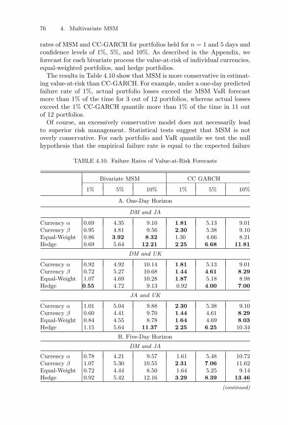
76 4. Multivariate MSM

rates of MSM and CC-GARCH for portfolios held for n = 1 and 5 days andconfidence levels of 1%, 5%, and 10%. As described in the Appendix, weforecast for each bivariate process the value-at-risk of individual currencies,equal-weighted portfolios, and hedge portfolios.

The results in Table 4.10 show that MSM is more conservative in estimat-ing value-at-risk than CC-GARCH. For example, under a one-day predictedfailure rate of 1%, actual portfolio losses exceed the MSM VaR forecastmore than 1% of the time for 3 out of 12 portfolios, whereas actual lossesexceed the 1% CC-GARCH quantile more than 1% of the time in 11 outof 12 portfolios.

Of course, an excessively conservative model does not necessarily leadto superior risk management. Statistical tests suggest that MSM is notoverly conservative. For each portfolio and VaR quantile we test the nullhypothesis that the empirical failure rate is equal to the expected failure

TABLE 4.10. Failure Rates of Value-at-Risk Forecasts

Bivariate MSM CC GARCH

1% 5% 10% 1% 5% 10%

A. One-Day Horizon

DM and JA

Currency α 0.69 4.35 9.10 1.81 5.13 9.01Currency β 0.95 4.81 9.56 2.30 5.38 9.10Equal-Weight 0.86 3.92 8.32 1.30 4.66 8.21Hedge 0.69 5.64 12.21 2.25 6.68 11.81

DM and UK

Currency α 0.92 4.92 10.14 1.81 5.13 9.01Currency β 0.72 5.27 10.68 1.44 4.61 8.29Equal-Weight 1.07 4.69 10.28 1.87 5.18 8.98Hedge 0.55 4.72 9.13 0.92 4.00 7.00

JA and UK

Currency α 1.01 5.04 9.88 2.30 5.38 9.10Currency β 0.60 4.41 9.70 1.44 4.61 8.29Equal-Weight 0.84 4.55 8.78 1.64 4.69 8.03Hedge 1.15 5.64 11.37 2.25 6.25 10.34

B. Five-Day Horizon

DM and JA

Currency α 0.78 4.21 9.57 1.61 5.48 10.72Currency β 1.07 5.30 10.55 2.31 7.06 11.62Equal-Weight 0.72 4.44 8.50 1.64 5.25 9.14Hedge 0.92 5.42 12.16 3.29 8.39 13.46

(continued)

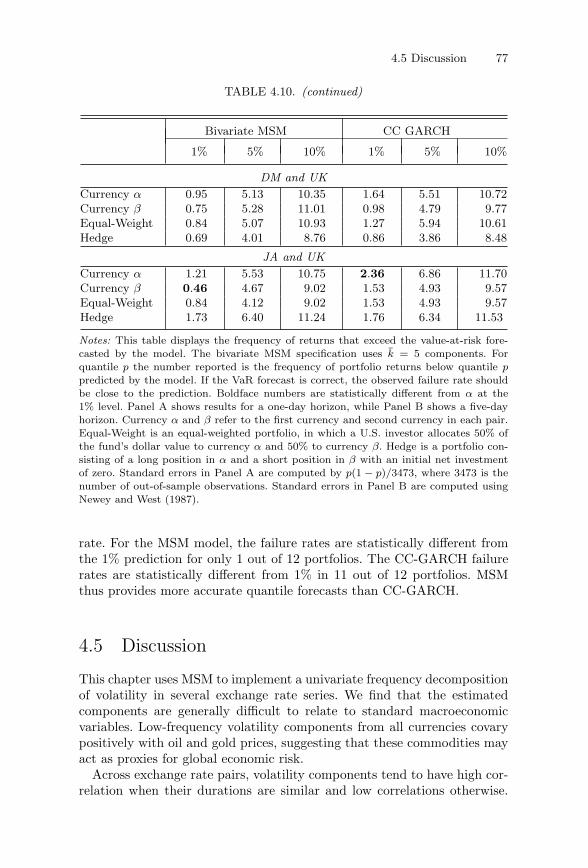
4.5 Discussion 77

TABLE 4.10. (continued)

Bivariate MSM CC GARCH

1% 5% 10% 1% 5% 10%

DM and UKCurrency α 0.95 5.13 10.35 1.64 5.51 10.72Currency β 0.75 5.28 11.01 0.98 4.79 9.77Equal-Weight 0.84 5.07 10.93 1.27 5.94 10.61Hedge 0.69 4.01 8.76 0.86 3.86 8.48

JA and UKCurrency α 1.21 5.53 10.75 2.36 6.86 11.70Currency β 0.46 4.67 9.02 1.53 4.93 9.57Equal-Weight 0.84 4.12 9.02 1.53 4.93 9.57Hedge 1.73 6.40 11.24 1.76 6.34 11.53

Notes: This table displays the frequency of returns that exceed the value-at-risk fore-casted by the model. The bivariate MSM specification uses k = 5 components. Forquantile p the number reported is the frequency of portfolio returns below quantile ppredicted by the model. If the VaR forecast is correct, the observed failure rate shouldbe close to the prediction. Boldface numbers are statistically different from α at the1% level. Panel A shows results for a one-day horizon, while Panel B shows a five-dayhorizon. Currency α and β refer to the first currency and second currency in each pair.Equal-Weight is an equal-weighted portfolio, in which a U.S. investor allocates 50% ofthe fund’s dollar value to currency α and 50% to currency β. Hedge is a portfolio con-sisting of a long position in α and a short position in β with an initial net investmentof zero. Standard errors in Panel A are computed by p(1 − p)/3473, where 3473 is thenumber of out-of-sample observations. Standard errors in Panel B are computed usingNewey and West (1987).

rate. For the MSM model, the failure rates are statistically different fromthe 1% prediction for only 1 out of 12 portfolios. The CC-GARCH failurerates are statistically different from 1% in 11 out of 12 portfolios. MSMthus provides more accurate quantile forecasts than CC-GARCH.

4.5 Discussion

This chapter uses MSM to implement a univariate frequency decompositionof volatility in several exchange rate series. We find that the estimatedcomponents are generally difficult to relate to standard macroeconomicvariables. Low-frequency volatility components from all currencies covarypositively with oil and gold prices, suggesting that these commodities mayact as proxies for global economic risk.

Across exchange rate pairs, volatility components tend to have high cor-relation when their durations are similar and low correlations otherwise.

78 4. Multivariate MSM

This finding motivates the development of bivariate MSM, a multifrequencymodel of comovement in stochastic volatility and covariation in financialprices. The model permits a parsimonious specification of bivariate shockswith heterogeneous durations, capturing the economic intuition that sharedfundamentals may have different innovation frequencies. Bayesian updat-ing and the likelihood function are always available in closed form, butare practical only when the state space is of moderate size. We developa particle filter suitable for larger state spaces, and demonstrate its goodperformance in inference and forecasting. Bivariate MSM performs wellin- and out-of-sample relative to a standard benchmark, CC-GARCH. Like-lihood ratio tests also confirm some of the principal restrictions of themodel. The bivariate MSM framework permits us to conduct inferenceand forecasting for good-performing pure regime-switching models with216 states and only eight parameters.

The bivariate MSM model investigated in this Chapter generalizes tothe multivariate case with many assets, as is discussed in the Appendix.We can consider either an arbitrary arrival correlation matrix across assetmarkets, which might be useful for applications with a relatively smallnumber of assets. Alternatively, we propose a factor model of multifre-quency stochastic volatility, which is specified by a number of volatilityparameters that grows linearly in the number of assets. Estimation can beconducted by maximizing the closed-form likelihood or by implementingthe particle filter methodology.

5Background: Continuous-TimeVolatility Modeling, Fractal Processes,and Multifractal Measures

This chapter provides background material for the continuous-timemultifractal volatility models that are fully developed in the remainderof Part II (Chapters 6–8), and in Chapter 10 of Part III. Our goal is notto survey the literature in any area, but to provide a brief introduction tothe continuous-time concepts employed in the rest of the book.

Much of the background information given here is directly useful tounderstanding the first multifractal diffusion, the MMAR. Specifically, timedeformation and multifractal measures are critical building blocks for theMMAR. The less directly related but nonetheless important self-similarprocesses, which have a long history in finance, are cousins of the multi-fractal diffusions considered in the remainder of Part II. The MMAR isdiscussed in Chapter 6.

Chapter 7 takes an alternative path to generating a multifractal diffu-sion by following continuous-time versions of the MSM processes developedin Chapter 3 to their weak limit. This approach bypasses the need towork with combinatorial multifractal measures constructed on a fixed grid.Continuous-time MSM has the same moment-scaling properties as theMMAR, and Chapter 8 confirms these predictions in currency and equitydata.

In this background review, we also briefly discuss jump-diffusion modelsof financial prices. Jump-diffusions are particularly relevant in Chapter 10,where we obtain endogenous discontinuities in prices and other appealingfeatures by using equilibrium valuation.

82 5. Background: Continuous-Time Volatility Modeling

5.1 Continuous-Time Models of Asset Prices

5.1.1 Brownian Motion, Time Deformation,and Jump-Diffusions

The Brownian motion (Bachelier, 1900) is the workhorse of continuous-time finance theory.1 Among many examples, Black and Scholes (1973)and Merton (1973) specify the log-price of a financial asset as a Brownianmotion with constant drift and volatility. While highly tractable in theore-tical applications, the Brownian motion representation assumes inde-pendent Gaussian increments and thus cannot capture the outliers andvolatility cycles exhibited by typical financial returns.

The Brownian motion is conveniently extended by considering deforma-tions of clock time, as suggested by Bochner (1949):

Definition 5.1 (Time deformation and compound process) Let{B(t)} be a stochastic process, and θ(t) an increasing function of clocktime t. We call

X(t) ≡ B[θ(t)]

a compound process, and θ(t) the trading time or time-deformationprocess.

When the process B is a martingale, innovations in trading time may speedup or slow down the process X(t) without influencing its direction. Com-pounding can thus separate the direction and the size of price movements,and has been used to model the unobserved natural time scale of eco-nomic series (Clark, 1973; Mandelbrot and Taylor, 1967; Stock, 1987, 1988).In Chapters 6 and 7, we show how compounding can be used to definemultifractal diffusions.

To account for thick tails in asset returns and the corresponding impliedvolatility smiles in near-maturity options, another approach used in con-tinuous time is to incorporate jumps in financial prices.2 For example,Merton (1976) assumes that the stock price follows an exogenous

1We refer the reader to Baxter and Rennie (1996), Bjork (2004), Cochrane (2005),Cont and Tankov (2003), Dana and Jeanblanc (2007), Dothan (1990), Duffie (1988,2001), Hunt and Kennedy (2004), Ingersoll (1987), Karatzas and Shreve (2001), Merton(1990), Musiela and Rutkowski (2007), Neftci (2000), Nielsen (1999), Shreve (2005), andWilmott (2006), among others, for excellent book length treatments of the continuous-time finance literature.

2Numerous studies provide evidence for jumps in the valuation of stocks and otherfinancial securities, based on the series of either the assets themselves or their derivativeclaims, against increasingly broad diffusion alternatives. See, for example, Ait-Sahalia(2002), Ait-Sahalia and Jacod (2008), Andersen, Benzoni, and Lund (2002), Andersen,

5.1 Continuous-Time Models of Asset Prices 83

jump-diffusion with constant volatility. Subsequent research considerseconometric refinements such as stochastic volatility, priced jumps, jumpsin volatility, correlation between jumps in returns and volatility, and infiniteactivity.3 Among numerous contributions, Bakshi, Cao, and Chen (1997)and Bates (2000) investigate price processes with exogenous jumps andstochastic volatility, and conclude that additional discontinuities in volatil-ity are necessary to match option valuations. Duffie, Pan, and Singleton(2000) analyze an extension with discrete volatility changes while exoge-nously specifying the relation between volatility and returns. A related lineof research (e.g., Madan, Carr, and Chang, 1998) considers pure jump pro-cesses characterized by infinite activity with many small events and fewerlarge discontinuities. In all of this literature, jumps in valuations and theirrelation to volatility are exogenously specified.4 In Chapter 10, we use equi-librium valuation to generate price jumps linked endogenously to volatilitychanges, and derive an inverse relation between the size and frequency ofprice discontinuities in a multifrequency environment.

5.1.2 Self-Similar (Fractal) ProcessesThe French mathematician Benoıt Mandelbrot has long recommendeddeparting from Ito diffusions in favor of adopting fat-tailed “fractal” pro-cesses. This alternative modeling approach builds on the concept of scaleinvariance. In a 1963 publication, Mandelbrot suggested that the shapeof the distribution of returns should be invariant when the time scale ischanged:

Definition 5.2 (Self-similar process) A random process {X(t)} thatsatisfies

{X(ct1), . . . , X (ctk)} d={cHX(t1), . . . , cHX(tk)

}

for some H > 0 and all c, k, t1, . . . , tk ≥ 0, is called self-similar orself-affine. The number H is the self-similarity index, or scaling exponent,of the process {X(t)}.

Bollerslev, and Diebold (2007), Ball and Torous (1985), Barndorff-Nielsen and Shephard(2004, 2006), Bates (1996, 2000), Carr, Geman, Madan, and Yor (2002), Carr and Wu(2003), Eraker (2004), Eraker, Johannes, and Polson (2003), Huang and Tauchen (2005),Jarrow and Rosenfeld (1984), Jorion (1988), Maheu and McCurdy (2004), and Press(1967).

3Jump processes are classified as having finite or infinite activity depending onwhether the number of jumps in a bounded time interval is finite or infinite.

4Other applications of jump processes in finance include Barndorff-Nielsen (1998),Eberlein, Keller, and Prause (1998), Liu, Pan, and Wang (2005), Naik and Lee (1990),and Pan (2002).

84 5. Background: Continuous-Time Volatility Modeling

The Brownian motion is self-similar with H = 1/2. Besides the Brownianmotion, the Levy-stable process and the fractional Brownian motion are themain examples of self-similar processes in finance. Embrechts and Maejima(2002), Mandelbrot (1997), and Samorodnitsky and Taqqu (1994) providethorough discussions of self-similar processes in finance and the naturalsciences, and we briefly review two important examples.

The stable processes of Paul Levy (1924) are characterized by fat tails inthe unconditional distribution of returns. They have been widely appliedin financial econometrics to model a variety of commodity, equity and cur-rency prices (e.g., Blattberg and Gonedes, 1974; Fama, 1963, 1965; Famaand Roll, 1971; Fielitz, 1976; Granger and Morgenstern, 1970; Koedijk andKool, 1992; Mandelbrot, 1963, 1967; Officer, 1972; Phillips, McFarland, andMcMahon, 1996; Samuelson, 1967, 1976). A problem with Levy-stable pro-cesses in financial applications is that they imply infinite variance, whichappears to be empirically inaccurate in typical financial data. Moreover,the Levy-stable model assumes that increments are independent throughtime, which is at odds with substantial empirical evidence of time-varyingvolatility.

The fractional Brownian motion (FBM), introduced by Kolmogorov(1940) and Mandelbrot (1965a), has continuous sample paths as wellas Gaussian and possibly dependent increments. A fractional Brownianmotion BH (t) is an ordinary Brownian motion for H = 1/2, is antiper-sistent when 0 < H < 1/2, and persistent with long memory in returnswhen 1/2 < H < 1. The FBM has been widely used in hydrology andclimatology, as reviewed in Samorodnitsky and Taqqu (1994). Applicationsin finance are limited by the fact that the FBM does not disentangle longmemory in volatility from long memory in returns. Chapters 6 and 7 showthat multifractal volatility modeling resolves this difficulty.

Empirical evidence suggests that many financial series are not self-similar, but instead have thinner tails and become less peaked in the bellswhen the sampling interval increases (e.g., Campbell, Lo, and MacKinlay,1996, Chapter 1). The volatility models in Chapters 6 and 7 capture thisnonlinearity, as well as thick tails and long-memory volatility persistence,by building on a generalized form of scaling that has been developed in themultifractal literature.

5.2 Multifractal Measures

The history of multifractals begins in the natural sciences, wheremultifractal measures have proven useful in numerous applications.5 We

5The literature on applications of multifractals includes wide-ranging contributionsacross many areas of study. A survey is beyond the scope of this book, but examplesinclude agronomy (Kravchenko, Bullock, and Boast, 2000; Zeleke and Si, 2004), astronomy

5.2 Multifractal Measures 85

now review the simplest multifractal, the binomial measure on a compactinterval, which generalizes to random multiplicative measures.

5.2.1 The Binomial MeasureFractals are sets that can be constructed by iterating a simple transfor-mation. Well-known examples include the Cantor set, which is constructedby recursively eliminating the middle third of intervals, or the Koch flake,which is obtained by recursively transforming segments into tent-shapedcurves. Mandelbrot (1982) provides a classic exposition of fractals and theirapplications in the natural sciences.

Analogous to fractal sets, multifractal measures are built by iteratinga simple transformation. The binomial measure6 on [0, 1] provides a sim-ple example, and is easily derived as the limit of a multiplicative cascade.Consider the uniform probability measure μ0 on the unit interval and twopositive numbers m0 and m1 adding up to 1. In the first step of the cas-cade, we define a measure μ1 by uniformly spreading the mass m0 on theleft subinterval [0, 1/2], and the mass m1 on the right subinterval [1/2, 1].The density of μ1 is a step function, as illustrated in Figure 5.1a.

In the second stage of the cascade, we split the interval [0, 1/2] intotwo subintervals of equal length. The left subinterval [0, 1/4] is allocateda fraction m0 of μ1[0, 1/2], while the right subinterval [1/4, 1/2] receives afraction m1. Applying a similar procedure to [1/2, 1], we obtain a measure

(Borgani, 1995; Jones et al., 1988, 2004; Martinez, 1999; Pietronero, 1987; Valdarnini,Borgani, and Provenzale, 1992), ecology (Borda-de-Agua, Hubbell, and MacAllister,2002; Drake and Weishampel, 2001; Kirkpatrick and Weishampel, 2005), geology andgeochemistry (Agterberg, 2007; Cheng, 1999; Cheng and Agterberg, 1995; de Wijs,1951; Goncalves, 2001; Paredes and Elorza, 1999; Xie and Bao, 2004), genetics (Gutier-rez, Rodriguez, and Abramson, 2001; Tino, 2002; Yu, Anh, and Lao, 2003), hydrology(Boufadel et al., 2000; Koscielny-Bunde et al., 2006; Labat, Mangin, and Ababou, 2002;Liu and Moltz, 1997; Pandey, Lovejoy, and Schertzer, 1998), meteorology (Carvalho,Lavallee, and Jones, 2002; Deidda, 2000; Lilley et al., 2006; Lovejoy and Schertzer, 2006;Olsson and Niemczynowicz, 1996; Schertzer and Lovejoy, 1987; Tessier, Lovejoy, andSchertzer, 1994), biology and medicine (Cornforth and Jelinek, 2008; Fernandez et al.,1999; Oprisan, Ardelean, and Frangopol, 2000; Smith, Lange, and Marks, 1996; Stojic,Reljin, and Reljin, 2006; Takahashi et al., 2004), network traffic modeling (Atzori, Aste,and Isola, 2006; Gilbert, Willinger, and Feldmann, 1999; Krishna, Gadre, and Desai,2003; Riedi et al., 1999), seismology (Geilikman, Golubeva, and Pisarenko, 1990; Godanoand Caruso, 1995; Nakaya and Hashimoto, 2002; Molchan and Kronrod, 2007; Sornetteand Ouillon, 2005), soil science (Dathe, Tarquis, and Perrier, 2006; Folorunso et al.,1994; Grout, Tarquis, and Wiesner, 1998; Martin and Montero, 2002; Posadas et al.,2003), and turbulence (Frisch and Parisi, 1985; Kolmogorov, 1962; Mandelbrot 1972,1974; Meneveau and Sreenivasan, 1987, 1991; Muzy, Bacry, and Arneodo, 1991; Yaglom,1966). For further discussion of some of these areas, see Davis et al. (1994), Mandelbrot(1989, 1999), Sornette (2004), and Stanley and Meakin (1988).

6The binomial is sometimes called the Bernoulli or Besicovitch measure.

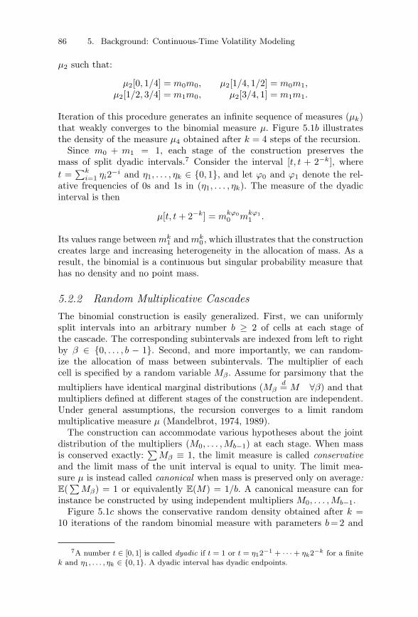
86 5. Background: Continuous-Time Volatility Modeling

μ2 such that:

μ2[0, 1/4] = m0m0, μ2[1/4, 1/2] = m0m1,μ2[1/2, 3/4] = m1m0, μ2[3/4, 1] = m1m1.

Iteration of this procedure generates an infinite sequence of measures (μk)that weakly converges to the binomial measure μ. Figure 5.1b illustratesthe density of the measure μ4 obtained after k = 4 steps of the recursion.

Since m0 + m1 = 1, each stage of the construction preserves themass of split dyadic intervals.7 Consider the interval [t, t + 2−k], wheret =

∑ki=1 ηi2−i and η1, . . . , ηk ∈ {0, 1}, and let ϕ0 and ϕ1 denote the rel-

ative frequencies of 0s and 1s in (η1, . . . , ηk). The measure of the dyadicinterval is then

μ[t, t + 2−k] = mkϕ00 mkϕ1

1 .

Its values range between mk1 and mk

0 , which illustrates that the constructioncreates large and increasing heterogeneity in the allocation of mass. As aresult, the binomial is a continuous but singular probability measure thathas no density and no point mass.

5.2.2 Random Multiplicative CascadesThe binomial construction is easily generalized. First, we can uniformlysplit intervals into an arbitrary number b ≥ 2 of cells at each stage ofthe cascade. The corresponding subintervals are indexed from left to rightby β ∈ {0, . . . , b − 1}. Second, and more importantly, we can random-ize the allocation of mass between subintervals. The multiplier of eachcell is specified by a random variable Mβ . Assume for parsimony that the

multipliers have identical marginal distributions (Mβd= M ∀β) and that

multipliers defined at different stages of the construction are independent.Under general assumptions, the recursion converges to a limit randommultiplicative measure μ (Mandelbrot, 1974, 1989).

The construction can accommodate various hypotheses about the jointdistribution of the multipliers (M0, . . . , Mb−1) at each stage. When massis conserved exactly:

∑Mβ ≡ 1, the limit measure is called conservative

and the limit mass of the unit interval is equal to unity. The limit mea-sure μ is instead called canonical when mass is preserved only on average:E(

∑Mβ) = 1 or equivalently E(M) = 1/b. A canonical measure can for

instance be constructed by using independent multipliers M0, . . . , Mb−1.Figure 5.1c shows the conservative random density obtained after k =

10 iterations of the random binomial measure with parameters b = 2 and

7A number t ∈ [0, 1] is called dyadic if t = 1 or t = η12−1 + · · · + ηk2−k for a finitek and η1, . . . , ηk ∈ {0, 1}. A dyadic interval has dyadic endpoints.

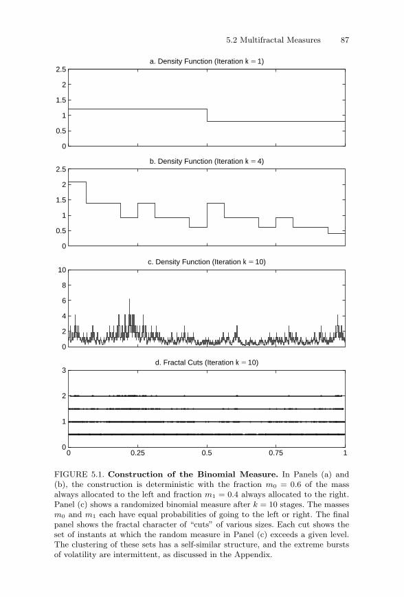
5.2 Multifractal Measures 87

0

0.5

1

1.5

2

2.5a. Density Function (Iteration k 5 1)

0

0.5

1

1.5

2

2.5b. Density Function (Iteration k 5 4)

0

2

4

6

8

10c. Density Function (Iteration k 5 10)

0 0.25 0.5 0.75 10

1

2

3d. Fractal Cuts (Iteration k 5 10)

FIGURE 5.1. Construction of the Binomial Measure. In Panels (a) and(b), the construction is deterministic with the fraction m0 = 0.6 of the massalways allocated to the left and fraction m1 = 0.4 always allocated to the right.Panel (c) shows a randomized binomial measure after k = 10 stages. The massesm0 and m1 each have equal probabilities of going to the left or right. The finalpanel shows the fractal character of “cuts” of various sizes. Each cut shows theset of instants at which the random measure in Panel (c) exceeds a given level.The clustering of these sets has a self-similar structure, and the extreme burstsof volatility are intermittent, as discussed in the Appendix.

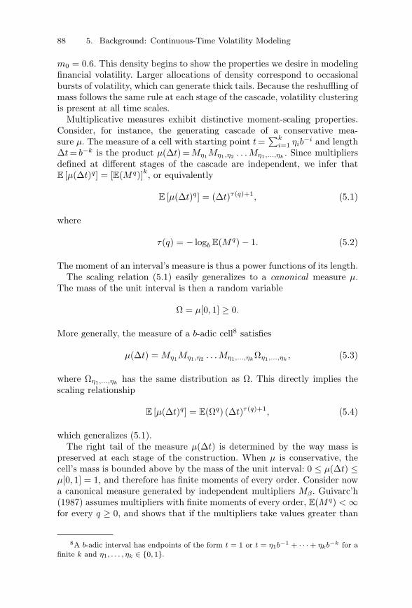
88 5. Background: Continuous-Time Volatility Modeling

m0 = 0.6. This density begins to show the properties we desire in modelingfinancial volatility. Larger allocations of density correspond to occasionalbursts of volatility, which can generate thick tails. Because the reshuffling ofmass follows the same rule at each stage of the cascade, volatility clusteringis present at all time scales.

Multiplicative measures exhibit distinctive moment-scaling properties.Consider, for instance, the generating cascade of a conservative mea-sure μ. The measure of a cell with starting point t =

∑ki=1 ηib

−i and lengthΔt = b−k is the product μ(Δt) = Mη1Mη1,η2 . . . Mη1,...,ηk

. Since multipliersdefined at different stages of the cascade are independent, we infer thatE [μ(Δt)q] = [E(Mq)]k, or equivalently

E [μ(Δt)q] = (Δt)τ(q)+1, (5.1)

where

τ(q) = − logb E(Mq) − 1. (5.2)

The moment of an interval’s measure is thus a power functions of its length.The scaling relation (5.1) easily generalizes to a canonical measure μ.

The mass of the unit interval is then a random variable

Ω = μ[0, 1] ≥ 0.

More generally, the measure of a b-adic cell8 satisfies

μ(Δt) = Mη1Mη1,η2 . . . Mη1,...,ηkΩη1,...,ηk

, (5.3)

where Ωη1,...,ηkhas the same distribution as Ω. This directly implies the

scaling relationship

E [μ(Δt)q] = E(Ωq) (Δt)τ(q)+1, (5.4)

which generalizes (5.1).The right tail of the measure μ(Δt) is determined by the way mass is

preserved at each stage of the construction. When μ is conservative, thecell’s mass is bounded above by the mass of the unit interval: 0 ≤ μ(Δt) ≤μ[0, 1] = 1, and therefore has finite moments of every order. Consider nowa canonical measure generated by independent multipliers Mβ . Guivarc’h(1987) assumes multipliers with finite moments of every order, E(Mq) < ∞for every q ≥ 0, and shows that if the multipliers take values greater than

8A b-adic interval has endpoints of the form t = 1 or t = η1b−1 + · · · + ηkb−k for afinite k and η1, . . . , ηk ∈ {0, 1}.

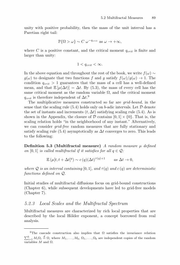
5.2 Multifractal Measures 89

unity with positive probability, then the mass of the unit interval has aParetian right tail:

P{Ω > ω} ∼ C ω−qcrit as ω → +∞,

where C is a positive constant, and the critical moment qcrit is finite andlarger than unity:

1 < qcrit < ∞.

In the above equation and throughout the rest of the book, we write f(ω) ∼g(ω) to designate that two functions f and g satisfy f(ω)/g(ω) → 1. Thecondition qcrit > 1 guarantees that the mass of a cell has a well-definedmean, and that E [μ(Δt)] = Δt. By (5.3), the mass of every cell has thesame critical moment as the random variable Ω, and the critical momentqcrit is therefore independent of Δt.9

The multiplicative measures constructed so far are grid-bound, in thesense that the scaling rule (5.4) holds only on b-adic intervals. Let D denotethe set of instants and increments (t, Δt) satisfying scaling rule (5.4). As isshown in the Appendix, the closure of D contains [0, 1] × {0}. That is, thescaling relation holds “in the neighborhood of any instant.” Alternatively,we can consider grid-free random measures that are fully stationary andsatisfy scaling rule (5.4) asymptotically as Δt converges to zero. This leadsto the following:

Definition 5.3 (Multifractal measure) A random measure μ definedon [0, 1] is called multifractal if it satisfies for all q ∈ Q:

E (μ[t, t + Δt]q) ∼ c (q)(Δt)τ(q)+1 as Δt → 0,

where Q is an interval containing [0, 1], and τ(q) and c (q) are deterministicfunctions defined on Q.

Initial studies of multifractal diffusions focus on grid-bound constructions(Chapter 6), while subsequent developments have led to grid-free models(Chapter 7).

5.2.3 Local Scales and the Multifractal SpectrumMultifractal measures are characterized by rich local properties that aredescribed by the local Holder exponent, a concept borrowed from realanalysis.

9The cascade construction also implies that Ω satisfies the invariance relation∑bi=1 MiΩi

d= Ω, where M1, . . . , Mb, Ω1, . . . , Ωb are independent copies of the randomvariables M and Ω.

90 5. Background: Continuous-Time Volatility Modeling

Definition 5.4 (Local Holder exponent) Let g be a function definedon the neighborhood of a given date t. The number

α(t) = Sup {β ≥ 0 : |g(t + t) − g(t)| = O(|t|β) as t → 0}

is called the local Holder exponent or local scale of g at t.

The Holder exponent describes the local variability of the function at apoint in time. Heuristically, we can express the infinitesimal variations ofthe function as being of order |dg| ≈ (dt)α(t) around instant t. Lower valuesof α(t) correspond to more abrupt variations. The exponent α(t) is non-negative when the function g is bounded around t, as is always the case inthis book. The definition readily extends to measures on the real line. Ata given date t, a measure simply has the local exponent of its cumulativedistribution function.

We can compute Holder exponents for many functions and processes.For instance, the local scale of a function is 0 at points of discontinuityand 1 at (nonsingular) differentiable points. On the other hand, the uniquescale α(t) = 1/2 is observed on the jagged sample paths of a Brownianmotion or of a continuous Ito diffusion.10 Similarly, a fractional BrownianBH(t) is characterized by a unique exponent α(t) = H. Thus, the continuousprocesses typically used in finance each have a unique Holder exponent. Incontrast, multifractal measures contain a continuum of local scales.

The mathematics literature has developed a convenient representation forthe distribution of Holder exponents in a multifractal. From Definition 5.4,the Holder exponent α(t) is the limit inferior of the ratio

ln |g(t,t)|/ ln(t) as t → 0,

where g(t,t) ≡ g(t+t)−g(t). This suggests estimating the distributionof the local scale α(t) at a random instant. For increasing k ≥ 1, we parti-tion the unit interval into bk subintervals [ti, ti + Δt] of length t = b−k,and calculate for each subinterval the coarse Holder exponent

αk(ti) ≡ ln |g(ti,t)|/ lnt.

This operation generates a set {αk(ti)} of bk observations.We divide the range of α’s into small intervals of length α, and denote

by Nk(α) the number of coarse exponents contained between α and α+α.It would then seem natural to calculate a histogram with the relativefrequencies Nk(α)/bk, which converge as k → ∞ to the probability that a

10More precisely, the set {t : α(t) �= 1/2} of instants with a local scale different from1/2 has a Hausdorff-Besicovitch measure (and therefore a Lebesgue measure) equal tozero. This set can thus be neglected in our analysis. See Kahane (1997) for a survey ofthis topic.

5.2 Multifractal Measures 91

random instant t has Holder exponent α. Using this method, the histogramwould degenerate into a spike because multifractals typically have a dom-inant exponent α0, in the sense that α(t) = α0 at almost every instant.Mandelbrot (1974, 1989) instead suggested

Definition 5.5 (Multifractal spectrum) The limit

f(α) ≡ lim(

lnNk(α)ln bk

)as k → ∞ (5.5)

represents a renormalized probability distribution of local Holder exponents,and is called the multifractal spectrum.

For instance if b = 3 and Nk(α) = 2k, the frequency Nk(α)/bk = (2/3)k

converges to zero as k → ∞, while the ratio lnNk(α)/ ln bk = ln 2/ ln 3 is apositive constant. The multifractal spectrum helps to identify events thathappen many times in the construction but at a vanishing frequency.

The quantity f(α) coincides with the fractal (or Hausdorff-Besicovitch)dimension of the set of instants having local Holder exponent α, T (α) ={t : α(t) = α}, as was shown by Frisch and Parisi (1985) and Halsey et al.(1986). For various levels of α, Figure 5.1d illustrates the subintervals withcoarse exponent αk(ti) < α. When the number of iterations k is sufficientlylarge, these “cuts” display a self-similar structure. The Appendix providesa more detailed discussion of this interpretation.

5.2.4 The Spectrum of Multiplicative MeasuresLarge Deviation Theory can be used to derive closed-form expressions forthe multifractal spectrum of multiplicative measures. Let μ denote a con-servative measure on the unit interval. The mass of a b-adic subinterval oflength Δt = b−k is the product μ[t, t + Δt] = Mη1Mη1,η2 . . . Mη1,...,ηk

. Thecoarse exponent αk(t) = lnμ[t, t + Δt]/ ln Δt can therefore be written asthe equal-weighted average

αk =1k

k∑

i=1

Vi, (5.6)

where Vi ≡ − logb Mη1,...,ηi . We interpret coarse Holder exponents as drawsof the random variable αk.

By the Strong Law of Large Numbers, αk converges almost surely to11

α0 = E(V1) = −E( logb M) > 1. (5.7)

11The relation −E ( logb M) > 1 follows from Jensen’s inequality and E (M) = 1/b.

92 5. Background: Continuous-Time Volatility Modeling

As k → ∞, almost all coarse exponents are contained in a small neigh-borhood of α0. Although the standard histogram Nk(α)/bk collapses to aspike at α0, the other coarse exponents are nonetheless important. In fact,most of the mass concentrates on intervals with Holder exponents that arebounded away from α0.12 Information on these “rare events” is containedin the tail of the random variable αk.

Tail behavior is the object of Large Deviation Theory. In 1938, HaraldCramer established the following theorem under conditions that weregradually weakened.

Proposition 2 (Cramer’s theorem) Let {Vk} denote a sequence of i.i.d.random variables. Then as k → ∞,

1k

ln P

{1k

k∑

i=1

Vi > α

}→ inf

q

(ln

[E eq(α−V1)

]), (5.8)

for any α > E(V1).

Proofs can be found in Billingsley (1979), Dembo and Zeitouni (1998), andvan der Vaart (1998).

Cramer’s theorem provides information about the tail behavior of coarseHolder exponents. We can apply (5.8) to (5.6), and infer that the tail distri-bution satisfies

1k

logb P (αk > α) → infq

[αq + logb E(Mq)].

As discussed in the Appendix, this limiting result implies:

Proposition 3 (Multifractal spectrum and scaling function) Themultifractal spectrum f(α) is the Legendre transform

f(α) = infq

[αq − τ(q)] (5.9)

of the scaling function τ(q).

This result holds for both conservative and canonical measures.The proposition leads immediately to explicit formulas for the spec-

trum. For instance, assume the multiplier distribution M is lognormal

12Let Tk denote the set of b-adic cells with local exponents greater than (1 + α0)/2.When k is large, Tk contains “almost all” cells, but its mass:

∑t∈Tk

(Δt)αk(t) ≤ bk(Δt)(α0+1)/2 = b−k(α0−1)/2

converges to zero as k goes to infinity.

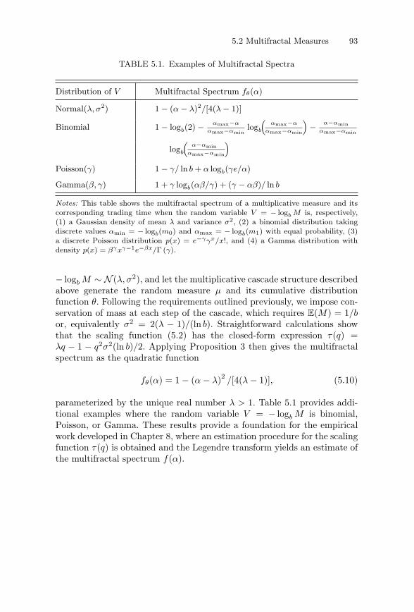
5.2 Multifractal Measures 93

TABLE 5.1. Examples of Multifractal Spectra

Distribution of V Multifractal Spectrum fθ(α)

Normal(λ, σ2) 1 − (α − λ)2/[4(λ − 1)]

Binomial 1 − logb(2) − αmax−α

αmax−αminlogb

(αmax−α

αmax−αmin

)− α−αmin

αmax−αmin

logb

(α−αmin

αmax−αmin

)

Poisson(γ) 1 − γ/ ln b + α logb(γe/α)

Gamma(β, γ) 1 + γ logb(αβ/γ) + (γ − αβ)/ ln b

Notes: This table shows the multifractal spectrum of a multiplicative measure and itscorresponding trading time when the random variable V = − logb M is, respectively,(1) a Gaussian density of mean λ and variance σ2, (2) a binomial distribution takingdiscrete values αmin = − logb(m0) and αmax = − logb(m1) with equal probability, (3)a discrete Poisson distribution p(x) = e−γγx/x!, and (4) a Gamma distribution withdensity p(x) = βγxγ−1e−βx/Γ (γ).

− logb M ∼ N (λ, σ2), and let the multiplicative cascade structure describedabove generate the random measure μ and its cumulative distributionfunction θ. Following the requirements outlined previously, we impose con-servation of mass at each step of the cascade, which requires E(M) = 1/bor, equivalently σ2 = 2(λ − 1)/(ln b). Straightforward calculations showthat the scaling function (5.2) has the closed-form expression τ(q) =λq − 1 − q2σ2(ln b)/2. Applying Proposition 3 then gives the multifractalspectrum as the quadratic function

fθ(α) = 1 − (α − λ)2 /[4(λ − 1)], (5.10)

parameterized by the unique real number λ > 1. Table 5.1 provides addi-tional examples where the random variable V = − logb M is binomial,Poisson, or Gamma. These results provide a foundation for the empiricalwork developed in Chapter 8, where an estimation procedure for the scalingfunction τ(q) is obtained and the Legendre transform yields an estimate ofthe multifractal spectrum f(α).

6Multifractal Diffusions ThroughTime Deformation and the MMAR

This chapter shows that multifractal diffusions can be created bycompounding a standard Brownian motion with a multifractal time defor-mation. The resulting price process is a semimartingale with a finitevariance, which precludes investors from making arbitrage profits in thesense of Harrison and Kreps (1979). The multifractal time deformationalso implies that the moments of returns scale as a power function ofthe frequency of observation, a property that has been extensively docu-mented in many financial time series. The time deformation approach wasused to define the first multifractal diffusion with uncorrelated increments,the Multifractal Model of Asset Returns (“MMAR,” Calvet, Fisher, andMandelbrot, 1997), which is also reviewed in this chapter. We will discussin Chapter 7 another leading example, continuous-time MSM.

In the MMAR, the multifractal time deformation is the cumulativedistribution function (c.d.f.) of a random multiplicative cascade. Theconstruction produces the moment-scaling, thick tails, and long-memoryvolatility persistence exhibited by many financial time series. The MMARsubstantially improves on traditional fractal specifications. In addition tothe semimartingale property, the MMAR accommodates flexible tail behav-iors with the highest finite moment taking any value greater than two. Themodel also captures the nonlinear changes in the unconditional distributionof returns at various sampling frequencies, while retaining the parsimonyand tractability of fractal approaches.

The MMAR provides a fundamentally new class of stochastic processesfor financial applications. In particular, the multifractal model is a diffusionthat lies outside the class of Ito processes. While the sample paths of Itodiffusions vary locally as (dt)1/2, the MMAR generates the richer class(dt)α(t) with the local scale α(t) taking a continuum of values in any finiteinterval.

6.1 Multifractal Processes

Consistent with the definition of multifractal measures, we can define amultifractal process by its moment-scaling properties:

This chapter is based on an earlier paper: “Multifractality in Asset Returns: Theory andEvidence” (with A. Fisher), Review of Economics and Statistics, 84: 381–406, August 2002.

96 6. Multifractal Diffusions Through Time Deformation and the MMAR

Definition 6.1 (Multifractal process) A stochastic process {X(t)} iscalled multifractal if it has stationary increments and satisfies the momentscaling rule

E (|X(t + Δt) − X(t)|q) ∼ cX(q) (Δt)τX(q)+1 (6.1)

as Δt converges to zero.

The function τX(q) is called the scaling function. Setting q = 0 in condition(6.1), we see that all scaling functions have the same intercept τX(0) = −1.We verify in the Appendix that the scaling function τX(q) is weakly concave,a direct implication of Holder’s inequality.

A self-similar process has a linear scaling function τX(q). The invariancecondition X(t) d= tHX(1) implies E (|X(t)|q) = tHq

E (|X(1)|q), and thescaling rule (6.1) therefore holds with

τX(q) = Hq − 1.

Since the intercept τX(0) =−1 is fixed, a linear scaling function is fullydetermined by its slope H. For this reason, self-similar processes are oftencalled uniscaling or unifractal. As discussed in Chapter 5, self-similar pro-cesses do not capture the changing distribution of returns at differenthorizons that is typical of most financial data. In this book, we focus on mul-tiscaling processes, which have a nonlinear and therefore strictly concavescaling function τX(q).

6.2 Multifractal Time Deformation

We now show how multiscaling multifractal processes can be obtainedthrough time deformation. Consider the price of a financial asset P (t) ona bounded interval [0, T ], and define the log-price process

X(t) ≡ lnP (t) − lnP (0).

We model X(t) by compounding a Brownian motion with a multifractaltrading time:

Condition 1 X(t) is a compound process

X(t) ≡ B[θ(t)],

where B(t) is a Brownian motion, and θ(t) is a stochastic time deformation.

Condition 2 The time deformation θ(t) is the cumulative distributionfunction (c.d.f.) of a multifractal measure μ defined on [0, T ].

6.2 Multifractal Time Deformation 97

Condition 3 The processes {B(t)} and {θ(t)} are independent.

Condition 1 can be easily generalized to permit time deformation of thefractional Brownian motion BH(t), as we show in Section 6.4. Condition 2specifies trading time θ(t) = μ[0, t] as the c.d.f. of a multifractal measure.This is a general condition that nests a variety of specifications includingthe MMAR (Section 6.3) and continuous-time MSM (Chapter 7). By defi-nition of a multifractal measure (see Chapter 5), the critical moment oftrading time qcrit(θ) is greater than unity:

qcrit(θ) > 1.

Condition 3 ensures that the unconditional distribution of returns issymmetric. Weakening this assumption could allow correlation betweenvolatility and returns, as in EGARCH (Nelson, 1991) and Glosten,Jagannathan, and Runkle (1993). In Part III, we pursue an alternativeapproach to generating a link between volatility and prices by usingequilibrium valuation.

Under Conditions 1–3, the moments of the compound process aregiven by:

E [|X(t)|q] = E[θ(t)q/2]E [|B(1)|q]. (6.2)

By Definition 5.3, the trading time θ satisfies the relation E[θ(t)q]∼ cθ(q)tτθ(q)+1. Return moments therefore scale as a power function of thefrequency of observation:

E [|X(t)|q] ∼ cX(q)tτX(q)+1 as t → 0, (6.3)

where τX(q) = τθ(q/2) and cX(q) = cθ(q/2)E [|B(1)|q]. These results aresummarized by:

Proposition 4 (Multifractality of price process) The time-deformedlog-price X(t) is a multifractal process with scaling function τX(q) ≡τθ(q/2).

We note that the multifractal trading time θ controls the tails of theprice and return processes. By (6.2), the q-th moment of the log-priceexists if and only if the time deformation has a moment of order q/2,implying that

qcrit(X) = 2qcrit(θ) > 2.

Multifractal diffusions obtained as time-deformed Brownian motions thushave finite variance, but are otherwise consistent with a wide range ofpotential tail behaviors as we will observe in the examples below.

98 6. Multifractal Diffusions Through Time Deformation and the MMAR

A multifractal diffusion resulting from Conditions 1–3 also has anappealing autocorrelation structure:

Proposition 5 (Martingale property) The price {P (t)} is a semi-martingale with respect to its natural filtration, and the process {X(t)}is a martingale with finite variance and uncorrelated increments.

The assumptions thus imply that asset returns have a white spectrum,a property that has been extensively discussed in the market efficiencyliterature.1

Since the price P (t) is a semimartingale, stochastic integration can beused to calculate the gains from trading multifractal assets. Consider, forinstance, the two-asset economy consisting of the multifractal security withprice P (t), and a riskless bond with constant rate of return r. Follow-ing Harrison and Kreps (1979), we can analyze if arbitrage profits can bemade by frequently rebalancing a portfolio of these two securities. Thesemimartingale property of Proposition 5 directly implies

Proposition 6 (No arbitrage) There are no arbitrage opportunities inthe two-asset economy.

Thus, multifractal diffusions can be embedded in standard economiesand are consistent with the basic requirements of equilibrium valuation.Part III of this book considers equilibrium valuation in greater detail.

6.3 The Multifractal Model of Asset Returns

The Multifractal Model of Asset Returns (MMAR) is obtained as a specialcase of the time-deformation conditions above. Specifically, we narrow thesecond condition:

Condition 2 ’ (The MMAR) The trading time θ (t) is the cumulativedistribution function of a random multiplicative cascade μ.

The MMAR specification was developed and empirically investigated inCalvet, Fisher, and Mandelbrot (1997) and Calvet and Fisher (2002a). Wenow discuss some of its additional properties.

6.3.1 Unconditional Distribution of ReturnsTail behavior is controlled by the multiplicative cascade. If μ is conservative,trading time is bounded and the log-price has finite moments of every

1See Campbell, Lo, and MacKinlay (1997) for a discussion of these concepts.

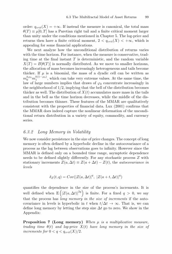
6.3 The Multifractal Model of Asset Returns 99

order: qcrit(X) = +∞. If instead the measure is canonical, the total massθ(T ) ≡ μ[0, T ] has a Paretian right tail and a finite critical moment largerthan unity under the conditions mentioned in Chapter 5. The log-price andreturns then have a finite critical moment, 2 < qcrit(X) < +∞, which isappealing for some financial applications.

We next analyze how the unconditional distribution of returns varieswith the time horizon. For instance, when the measure is conservative, trad-ing time at the final instant T is deterministic, and the random variableX(T ) = B[θ(T )] is normally distributed. As we move to smaller horizons,the allocation of mass becomes increasingly heterogeneous and tails becomethicker. If μ is a binomial, the mass of a dyadic cell can be written asmkϕ0

0 mk(1−ϕ0)1 , which can take very extreme values. At the same time, the

law of large numbers implies that draws of ϕ0 concentrate increasingly inthe neighborhood of 1/2, implying that the bell of the distribution becomesthicker as well. The distribution of X(t) accumulates more mass in the tailsand in the bell as the time horizon decreases, while the middle of the dis-tribution becomes thinner. These features of the MMAR are qualitativelyconsistent with the properties of financial data. Lux (2001) confirms thatthe MMAR does indeed capture the nonlinear deformation of the uncondi-tional return distribution in a variety of equity, commodity, and currencyseries.

6.3.2 Long Memory in VolatilityWe now consider persistence in the size of price changes. The concept of longmemory is often defined by a hyperbolic decline in the autocovariance of aprocess as the lag between observations goes to infinity. However since theMMAR is defined only on a bounded time range, asymptotic dependenceneeds to be defined slightly differently. For any stochastic process Z withstationary increments Z(a,Δt) ≡ Z(a + Δt) − Z(t), the autocovariance inlevels

δZ(t, q) = Cov(|Z(a,Δt)|q, |Z(a + t, Δt)|q)

quantifies the dependence in the size of the process’s increments. It iswell defined when E

(|Z(a,Δt)|2q

)is finite. For a fixed q > 0, we say

that the process has long memory in the size of increments if the auto-covariance in levels is hyperbolic in t when t/Δt → ∞. That is, we candefine long memory by letting the step size Δt go to zero. We show in theAppendix:

Proposition 7 (Long memory) When μ is a multiplicative measure,trading time θ(t) and log-price X(t) have long memory in the size ofincrements for 0 < q < qcrit(X)/2.

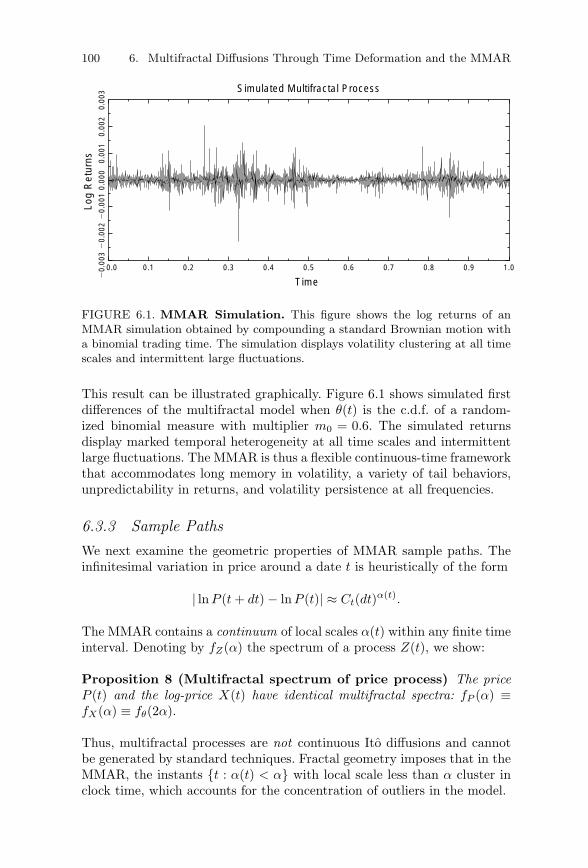
100 6. Multifractal Diffusions Through Time Deformation and the MMAR

Simulated Multifractal ProcessLo

g R

etur

ns

Time0.0

20.

003

20.

002

20.

001

0.00

00.

001

0.00

20.

003

0.1 0.2 0.3 0.4 0.5 0.6 0.7 0.8 0.9 1.0

FIGURE 6.1. MMAR Simulation. This figure shows the log returns of anMMAR simulation obtained by compounding a standard Brownian motion witha binomial trading time. The simulation displays volatility clustering at all timescales and intermittent large fluctuations.

This result can be illustrated graphically. Figure 6.1 shows simulated firstdifferences of the multifractal model when θ(t) is the c.d.f. of a random-ized binomial measure with multiplier m0 = 0.6. The simulated returnsdisplay marked temporal heterogeneity at all time scales and intermittentlarge fluctuations. The MMAR is thus a flexible continuous-time frameworkthat accommodates long memory in volatility, a variety of tail behaviors,unpredictability in returns, and volatility persistence at all frequencies.

6.3.3 Sample PathsWe next examine the geometric properties of MMAR sample paths. Theinfinitesimal variation in price around a date t is heuristically of the form

| lnP (t + dt) − lnP (t)| ≈ Ct(dt)α(t).

The MMAR contains a continuum of local scales α(t) within any finite timeinterval. Denoting by fZ(α) the spectrum of a process Z(t), we show:

Proposition 8 (Multifractal spectrum of price process) The priceP (t) and the log-price X(t) have identical multifractal spectra: fP (α) ≡fX(α) ≡ fθ(2α).

Thus, multifractal processes are not continuous Ito diffusions and cannotbe generated by standard techniques. Fractal geometry imposes that in theMMAR, the instants {t : α(t) < α} with local scale less than α cluster inclock time, which accounts for the concentration of outliers in the model.

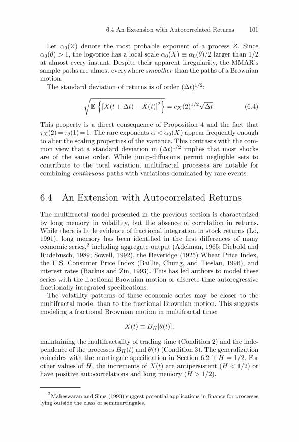
6.4 An Extension with Autocorrelated Returns 101

Let α0(Z) denote the most probable exponent of a process Z. Sinceα0(θ) > 1, the log-price has a local scale α0(X) ≡ α0(θ)/2 larger than 1/2at almost every instant. Despite their apparent irregularity, the MMAR’ssample paths are almost everywhere smoother than the paths of a Brownianmotion.

The standard deviation of returns is of order (Δt)1/2:√

E

{[X(t + Δt) − X(t)]2

}= cX(2)1/2

√Δt. (6.4)

This property is a direct consequence of Proposition 4 and the fact thatτX(2) = τθ(1) = 1. The rare exponents α < α0(X) appear frequently enoughto alter the scaling properties of the variance. This contrasts with the com-mon view that a standard deviation in (Δt)1/2 implies that most shocksare of the same order. While jump-diffusions permit negligible sets tocontribute to the total variation, multifractal processes are notable forcombining continuous paths with variations dominated by rare events.

6.4 An Extension with Autocorrelated Returns

The multifractal model presented in the previous section is characterizedby long memory in volatility, but the absence of correlation in returns.While there is little evidence of fractional integration in stock returns (Lo,1991), long memory has been identified in the first differences of manyeconomic series,2 including aggregate output (Adelman, 1965; Diebold andRudebusch, 1989; Sowell, 1992), the Beveridge (1925) Wheat Price Index,the U.S. Consumer Price Index (Baillie, Chung, and Tieslau, 1996), andinterest rates (Backus and Zin, 1993). This has led authors to model theseseries with the fractional Brownian motion or discrete-time autoregressivefractionally integrated specifications.

The volatility patterns of these economic series may be closer to themultifractal model than to the fractional Brownian motion. This suggestsmodeling a fractional Brownian motion in multifractal time:

X(t) ≡ BH [θ(t)],

maintaining the multifractality of trading time (Condition 2) and the inde-pendence of the processes BH(t) and θ(t) (Condition 3). The generalizationcoincides with the martingale specification in Section 6.2 if H = 1/2. Forother values of H, the increments of X(t) are antipersistent (H < 1/2) orhave positive autocorrelations and long memory (H > 1/2).

2Maheswaran and Sims (1993) suggest potential applications in finance for processes

lying outside the class of semimartingales.

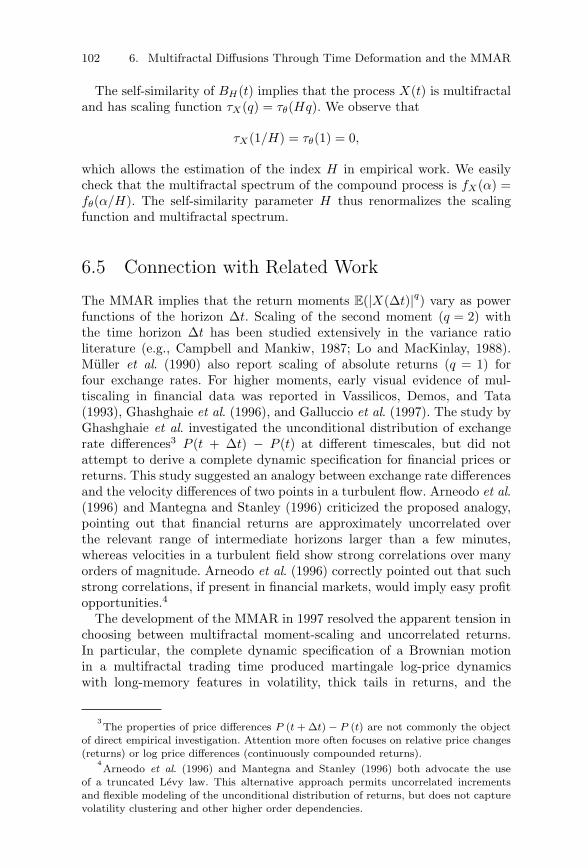
102 6. Multifractal Diffusions Through Time Deformation and the MMAR

The self-similarity of BH(t) implies that the process X(t) is multifractaland has scaling function τX(q) = τθ(Hq). We observe that

τX(1/H) = τθ(1) = 0,

which allows the estimation of the index H in empirical work. We easilycheck that the multifractal spectrum of the compound process is fX(α) =fθ(α/H). The self-similarity parameter H thus renormalizes the scalingfunction and multifractal spectrum.

6.5 Connection with Related Work

The MMAR implies that the return moments E(|X(Δt)|q) vary as powerfunctions of the horizon Δt. Scaling of the second moment (q = 2) withthe time horizon Δt has been studied extensively in the variance ratioliterature (e.g., Campbell and Mankiw, 1987; Lo and MacKinlay, 1988).Muller et al. (1990) also report scaling of absolute returns (q = 1) forfour exchange rates. For higher moments, early visual evidence of mul-tiscaling in financial data was reported in Vassilicos, Demos, and Tata(1993), Ghashghaie et al. (1996), and Galluccio et al. (1997). The study byGhashghaie et al. investigated the unconditional distribution of exchangerate differences3 P (t + Δt) − P (t) at different timescales, but did notattempt to derive a complete dynamic specification for financial prices orreturns. This study suggested an analogy between exchange rate differencesand the velocity differences of two points in a turbulent flow. Arneodo et al.(1996) and Mantegna and Stanley (1996) criticized the proposed analogy,pointing out that financial returns are approximately uncorrelated overthe relevant range of intermediate horizons larger than a few minutes,whereas velocities in a turbulent field show strong correlations over manyorders of magnitude. Arneodo et al. (1996) correctly pointed out that suchstrong correlations, if present in financial markets, would imply easy profitopportunities.4

The development of the MMAR in 1997 resolved the apparent tension inchoosing between multifractal moment-scaling and uncorrelated returns.In particular, the complete dynamic specification of a Brownian motionin a multifractal trading time produced martingale log-price dynamicswith long-memory features in volatility, thick tails in returns, and the

3The properties of price differences P (t + Δt) − P (t) are not commonly the object

of direct empirical investigation. Attention more often focuses on relative price changes(returns) or log price differences (continuously compounded returns).

4Arneodo et al. (1996) and Mantegna and Stanley (1996) both advocate the use

of a truncated Levy law. This alternative approach permits uncorrelated incrementsand flexible modeling of the unconditional distribution of returns, but does not capturevolatility clustering and other higher order dependencies.

6.6 Discussion 103

moment-scaling properties that characterize multifractals. Furthermore,this definition of a multifractal price process permitted the recovery ofa realistic stochastic generating mechanism that was simulated and com-pared with other competing models of returns. These informal MonteCarlo tests were made rigorous in Calvet and Fisher (2002a) by using aglobal test statistic based on simulated moments, as will be discussed inChapter 8.

6.6 Discussion

Time deformation provides a powerful tool to construct multifractal pro-cesses out of general multifractal measures. The first example of thistechnique in the literature is the Multifractal Model of Asset Returns,which incorporates the outliers and volatility persistence exhibited bymany financial time series, as well as a rich pattern of local variationsand moment-scaling properties.

The MMAR provides a fundamentally new class of diffusions to bothfinance and mathematics. These diffusions have potentially uncorrelatedincrements and continuous sample paths but lie outside the Ito class.Whereas standard processes can be characterized by a single local scale thatdescribes the local growth rate of variation, sample paths of multifractalprocesses contain a continuum of local Holder exponents within any timeinterval.

The main drawback of the MMAR is that the construction of tradingtime on a grid results in a nonstationary model, which creates an obsta-cle for typical financial applications such as volatility forecasting. Thenext chapter corrects this difficulty by randomizing the instants at whichvolatility components change.

7Continuous-Time MSM

This chapter develops the Markov-Switching Multifractal in continuoustime. Consistent with the discrete-time construction in Chapter 3, wespecify volatility at a given instant t as the multiplicative product of afinite number of random components. A Poisson process of fixed intensityγk can trigger switches in a given volatility component k, and heteroge-neous frequencies are parsimoniously incorporated into the construction byassuming that the arrival intensities γk follow a tight geometric progres-sion. Continuous-time MSM is naturally defined on an unbounded timedomain, which is a substantial improvement over the MMAR. It also gen-erates volatility clustering on a wide frequency range, corresponding to theintuition that economic factors such as technology shocks, business andearnings cycles, and liquidity shocks have different time scales.

When the number of components goes to infinity, the limiting price pro-cess displays complex features. Local volatility becomes degenerate, butthe time-deformation process is a positive martingale that has a nonde-generate quadratic variation over finite intervals. As in the MMAR, thelimit multifractal time deformation generates continuous sample paths withclustering and long memory in volatility. Furthermore, continuous-timeMSM improves on the MMAR by producing strictly stationary increments,which is crucial to facilitate estimation and forecasting in common financialapplications.

We complete the link with the discrete-time MSM processes developedin Chapter 3 by showing that an appropriately chosen sequence of discreteprocesses weakly converges to continuous-time MSM as the grid step sizegoes to zero. This ensures that the discrete model provides a consistent setof filters for continuous-time MSM. The chapter thus demonstrates thatthe Markov-switching approach works equally well in discrete time and incontinuous time, and that it is straightforward to go back and forth betweenthe two formulations.

We close the chapter by discussing the link between MSM and recentrelated stochastic volatility approaches that have been developed in thephysics, mathematics, and econometrics literatures.

This chapter is based on an earlier paper: “Forecasting Multifractal Volatility” (withA. Fisher), Econometrics, 105: 27–58, November 2006.

106 7. Continuous-Time MSM

7.1 MSM with Finitely Many Components

This section introduces a grid-free multifrequency diffusion. Analogous tothe approach discussed in Chapter 3, the continuous-time construction isbased on the Markov state vector

Mt = (M1,t;M2,t; . . . ;Mk,t) ∈ Rk+, t ∈ [0,+∞).

Given the Markov state Mt at date t, the dynamics over an infinitesimalinterval are defined as follows. For each k ∈ {1, . . . , k}, a change in Mk,t

may be triggered by a Poisson arrival with intensity γk:

Mk,t+dt drawn from distribution M with probability γkdtMk,t+dt = Mk,t with probability 1 − γkdt.

The Poisson arrivals and new draws from M are independent across k andt. As with any process driven by Poisson arrivals, the sample paths of acomponent Mk,t are cadlag, that is, are right-continuous and have a limitpoint to the left of any instant.1 The construction can accommodate anydistribution M with unit mean and positive support.

The arrival intensities follow the geometric progression:

γk = γ1bk−1, k ∈ {1, . . . , k}. (7.1)

The parameter γ1 determines the persistence of the lowest frequency com-ponent, and b > 1 the spacing between component frequencies. The inten-sity sequence is thus exactly geometric in continuous time, and in theAppendix we show that its discretization on a time grid leads to thediscrete-time definition (3.2).

The log-price X (t) = lnP (t) − lnP (0) has a constant drift g andstochastic volatility

σ(Mt) ≡ σ

⎛

⎝k∏

k=1

Mk,t

⎞

⎠1/2

, (7.2)

where σ is a positive constant. The process X(t) is formally defined as

Xt ≡ gt +∫ t

0σ(Ms)dZ(s),

where Z is a standard Brownian. The stochastic integral exists sinceE

[∫ t

0 σ2(Ms)ds]

= σ2t < ∞. Equivalently, the log-price satisfies the

1Cadlag is a French acronym for continue a droite, limites a gauche. We refer the

reader to Billingsley (1999) for further details.

7.2 MSM with Countably Many Components 107

stochastic differential equation

dXt ≡ gdt + σ(Mt)dZ(t). (7.3)

Continuous-time MSM is fully specified by the distribution M and theparameters (g, σ, γ1, b). It has strictly stationary increments, and thusresolves the grid-bound nonstationarity of the MMAR. Continuous-timeMSM can be easily integrated into an equilibrium framework, as will beshown in Chapter 10.

Figure 7.1 illustrates the construction when the distribution M is abinomial. The top panel shows the lowest frequency component M1,t, thesecond panel shows the product M1,tM2,t, and the third panel, σ2(Mt) ≡σ2M1,tM2,t . . . Mk,t, where σ = 1 and k = 12. The fourth and fifth panelsdisplay the corresponding returns and prices. The returns show pronouncedpeaks and intermittent bursts of volatility, accommodating a broad rangeof long-run, medium-run, and short-run dynamics.

Continuous-time MSM provides a parsimonious diffusion with Markov-switching volatility and multiple frequencies. The model fits naturallywithin the finance literature on Ito diffusions and regime-switching whenthe number of frequencies is finite. In particular, we can then apply toMSM all the tools that have been developed for general Markov processes(e.g., Ethier and Kurtz, 1986; Rogers and Williams, 2000). The model alsoeasily extends to the multivariate case, as is discussed in the Appendix.

7.2 MSM with Countably Many Components

In this section, we investigate how the price diffusion evolves as k → ∞and components of increasingly high frequency are added into the statevector. Two apparently contradictory observations can be made. On theone hand, Figure 7.1 suggests that the volatility process σ(Mt) exhibitsincreasingly extreme behavior as k increases. On the other hand, the priceprocess appears relatively insensitive to higher-frequency components. Wenow show how these two observations can be reconciled by deriving thelimit behavior of the price dynamics.

7.2.1 Limiting Time DeformationLet Mt = (Mk,t)∞

k=1 ∈ R∞+ be an MSM state process with countably many

frequencies, parameters (g, σ, γ1, b), and fixed multiplier distribution M .The process Mt is defined for t ∈ [0,∞), and has mutually independentcomponents. Each component Mk,t is characterized by the arrival intensityγk = γ1b

k−1. For a finite k, stochastic volatility is the product of the firstk components of the state vector: σk(Mt) ≡ σ(M1,tM2,t . . . Mk,t)1/2.

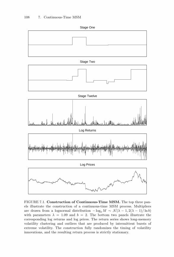
108 7. Continuous-Time MSM

Stage One

Stage Two

Stage Twelve

Log Returns

Log Prices

FIGURE 7.1. Construction of Continuous-Time MSM. The top three pan-els illustrate the construction of a continuous-time MSM process. Multipliersare drawn from a lognormal distribution − logb M ∼ N (λ − 1, 2(λ − 1)/ ln b)with parameters λ = 1.09 and b = 2. The bottom two panels illustrate thecorresponding log returns and log prices. The return series shows long-memoryvolatility clustering and outliers that are produced by intermittent bursts ofextreme volatility. The construction fully randomizes the timing of volatilityinnovations, and the resulting return process is strictly stationary.

7.2 MSM with Countably Many Components 109

Since instantaneous volatility σk(Mt) depends on an increasing numberof components, the differential representation (7.3) becomes unwieldyas k → ∞. We instead characterize dividend dynamics by the timedeformation

θk(t) ≡∫ t

0σ2

k(Ms)ds. (7.4)

Given a fixed instant t, the sequence {θk(t)}∞k=1 is a positive martingale

with bounded expectation. By the martingale convergence theorem, therandom variable θk(t) converges to a limit distribution when k → ∞.A similar argument applies to any vector sequence {θk(t1); . . . ; θk(td)},guaranteeing that the stochastic process θk has at most one limit point.

We verify that a limit process does indeed exist by checking that thesequence (θk)k is tight2 on any bounded time interval [0, T ]. Intuitively,tightness prevents the process from oscillating too wildly as k → ∞. Weassume

Condition 4 E(M2) < b.

which restricts fluctuations in the time deformation by requiring thatvolatility shocks be sufficiently small or have durations decreasing suffi-ciently fast. In the Appendix we prove:

Proposition 9 (Time deformation with countably manyfrequencies) Under Condition 4, the sequence (θk)k weakly converges toa process θ∞ in the space of continuous functions on [0, T ]. Furthermore,supk E

[θ2

k(t)]

< ∞ for every fixed t.

Additional intuition is gained by considering why we work with the time-deformation process θ∞ rather than attempt to take the pointwise limitof the integrand σ2

k(Mt) in Equation (7.4). By the Law of Large Numbers,

σ2k(Ms) = exp (

∑k lnMk,s) converges almost surely to zero as k→∞, which

might suggest that the limit trading time θ∞ degenerates to zero. In fact,the limit trading time θ∞ is not zero, which can be confirmed by notingthat for every fixed t > 0, E [θk(t)] = σ2t, supk E

[θ2

k(t)

]< ∞, and therefore

E [θ∞(t)] = σ2t > 0.

To understand why the trading time θ∞ remains positive even thoughvolatility σk(Mt) goes to zero almost surely as k → ∞, consider theimportance of rare events. On any finite interval, large realizations of

2We refer the reader to Billingsley (1999), Pollard (1984), and Davidson (1994) for

book-length treatments of the weak convergence of stochatic processes.

110 7. Continuous-Time MSM

volatility σk(Mt) appear sufficiently frequently to guarantee that the inte-gral (7.4) does not vanish. The trading time of continuous-time MSM thusprovides an example in which the Lebesgue dominated convergence theo-rem does not apply. The importance of rare events for the trading timeθ∞ will have natural consequences for the local variations of MSM samplepaths, as we will discuss in the next subsection.

Trading time θ∞(t) exhibits moment-scaling for small values of t. Weprove in the Appendix:

Proposition 10 (Moment scaling) The qth moment of trading timesatisfies

E {[θ∞(t)q]} ∼ cqtτθ(q)+1 as t → 0

where τθ(q) = − logb [E(Mq)] + q − 1 and cq is a positive constant.

The scaling function τθ(q) is concave by Holder’s inequality.3

Trading time is easily extended to the infinite time domain [0,∞). Con-sider the space D[0,∞) of cadlag functions defined on [0,∞), and let d◦

∞denote the Skorohod distance. Proposition 9 then directly leads to:

Corollary 1 (Unbounded time domain) If E(M2) < b, the sequence(θk)k weakly converges as k → ∞ to a measure θ∞ defined on the metricspace (D[0,∞), d◦

∞). The sample paths of θ∞ are continuous almost surely.

The ability to define trading time over an unbounded interval is a sub-stantial advantage of the Markov construction over the MMAR.

7.2.2 Multifractal Price DiffusionAs components of increasingly high frequencies are added into the statevector, the MSM diffusions considered in Section 7.1 converge to a weaklimit, which can be represented by X(t) ≡ gt + B[θ∞(t)]. The processes{B(t)} and {θ∞(t)} are again independent, and:

Condition 2” (Continuous-time MSM) The trading time θ∞ is anMSM time deformation with countably many frequencies.

The limiting MSM diffusion X(t) improves on the MMAR in two relatedways. First, the new model is a grid-free process in which volatility compo-nents switch at random instants and not at predetermined points of time.Second, X(t) can be interpreted as a stochastic volatility model with aMarkov latent state defined on an unbounded time domain.

3The multiplier satisfies the normalization conditions E(M) = 1/b in the MMAR and

E(M) = 1 in MSM. This leads to slightly different relations between τθ(q) and E(Mq).

7.2 MSM with Countably Many Components 111

In addition to these improvements, the limiting MSM diffusion sharesmany of the appealing properties of the MMAR. The compound processB[θ∞(t)] is a martingale because the increments of the Brownian motionB have unpredictable signs. The price process P (t) = exp[X(t)] is thena semimartingale, which precludes arbitrage in the presence of a risk-freebond. The scaling properties of trading time given in Proposition 10 implythat returns satisfy asymptotic moment scaling:

E [|X(t)|q] ∼ CqtτX(q)+1 as t → 0, (7.5)

where τX(q) ≡ τθ(q/2).4 Figure 7.2 uses Monte Carlo simulations to showthat this property also holds remarkably well for finite time increments.In the next chapter, we show that many financial time series, includingexchange rates and equities, exhibit moment-scaling.

Another important feature captured by MSM is long memory in volatil-ity. In Chapter 6, we introduced a quantitative description of long memoryfor a continuous-time process defined on a bounded time interval. Con-sistent with this approach, we show in Figure 7.3 that autocovariances ofsquared returns decline hyperbolically in simulated MSM data.

Finally, following the discussion of the importance of rare events totrading time in the previous subsection, the local variations of MSM arealmost everywhere smoother than the (dt)1/2 variations of an Ito process.Furthermore, despite continuity of the sample paths most of the varia-tion within any finite interval occurs on a set of instants with Lebesguemeasure zero. Thus, analogous to the quadratic variations (6.4) of theMMAR discussed previously, “rare events” are important to understandingthe variations of continuous-time MSM.

7.2.3 Connection between Discrete-Time andContinuous-Time Versions of MSM

We now analyze how continuous-time MSM relates to the discrete-timemodel presented in Chapter 3. Specifically, we establish that a rescaledversion of discrete-time MSM converges to continuous-time MSM whenthe number of frequencies goes to infinity.

Consider the following definitions:

Continuous-Time Construction. We continue to denote by θ∞ an MSMtrading time defined on a bounded interval [0, T ]. It is specified by (σ, γ1, b)and a fixed distribution M. We also assume that there exists q > 0 suchthat τθ(q) > 0.5

4If the drift g differs from zero, the scaling rule holds if τ(q) + 1 < q. Violations

of this inequality occur on an interval [0, q], q < 2, when the distribution M satisfiesE(logb M) < −1.

5This property holds under Condition 4 because one can easily check that τθ(q) is

strictly positive for q = 2 if and only if E(M2) < b. More generally, since τθ(1) = 0, the

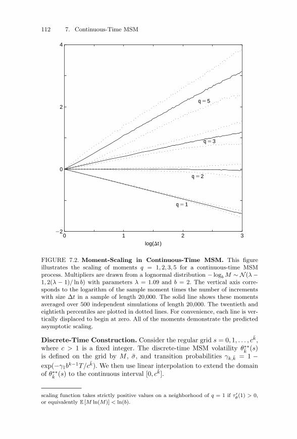
112 7. Continuous-Time MSM

0 1 2 322

0

2

4

log(Dt )

q 5 1

q 5 2

q 5 3

q 5 5

FIGURE 7.2. Moment-Scaling in Continuous-Time MSM. This figureillustrates the scaling of moments q = 1, 2, 3, 5 for a continuous-time MSMprocess. Multipliers are drawn from a lognormal distribution − logb M ∼ N (λ −1, 2(λ − 1)/ ln b) with parameters λ = 1.09 and b = 2. The vertical axis corre-sponds to the logarithm of the sample moment times the number of incrementswith size Δt in a sample of length 20,000. The solid line shows these momentsaveraged over 500 independent simulations of length 20,000. The twentieth andeightieth percentiles are plotted in dotted lines. For convenience, each line is ver-tically displaced to begin at zero. All of the moments demonstrate the predictedasymptotic scaling.

Discrete-Time Construction. Consider the regular grid s = 0, 1, . . . , ck,where c > 1 is a fixed integer. The discrete-time MSM volatility θ∗∗

k(s)

is defined on the grid by M , σ, and transition probabilities γk,k = 1 −exp(−γ1b

k−1T/ck). We then use linear interpolation to extend the domainof θ∗∗

k(s) to the continuous interval [0, ck].

scaling function takes strictly positive values on a neighborhood of q = 1 if τ ′θ(1) > 0,

or equivalently E [M ln(M)] < ln(b).

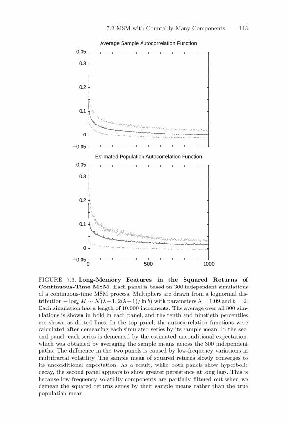
7.2 MSM with Countably Many Components 113

Average Sample Autocorrelation Function

20.05

0

0.1

0.2

0.3

0.35

0 500 1000

Estimated Population Autocorrelation Function

20.05

0

0.1

0.2

0.3

0.35

FIGURE 7.3. Long-Memory Features in the Squared Returns ofContinuous-Time MSM. Each panel is based on 300 independent simulationsof a continuous-time MSM process. Multipliers are drawn from a lognormal dis-tribution − logb M ∼ N (λ−1, 2(λ−1)/ ln b) with parameters λ = 1.09 and b = 2.Each simulation has a length of 10,000 increments. The average over all 300 sim-ulations is shown in bold in each panel, and the tenth and ninetieth percentilesare shown as dotted lines. In the top panel, the autocorrelation functions werecalculated after demeaning each simulated series by its sample mean. In the sec-ond panel, each series is demeaned by the estimated unconditional expectation,which was obtained by averaging the sample means across the 300 independentpaths. The difference in the two panels is caused by low-frequency variations inmultifractal volatility. The sample mean of squared returns slowly converges toits unconditional expectation. As a result, while both panels show hyperbolicdecay, the second panel appears to show greater persistence at long lags. This isbecause low-frequency volatility components are partially filtered out when wedemean the squared returns series by their sample means rather than the truepopulation mean.

114 7. Continuous-Time MSM

Rescaled Version. The discretized trading time θ∗k

is defined on the timeinterval [0, T ] by

θ∗k(t) = θ∗∗

k (tck/T ).

The process θ∗k

is continuous and piecewise linear.

We provide two alternative conditions under which the sequence oftrading times {θ∗

k}∞

k=1 weakly converge to the process θ∞.

Condition 5 b < c.

Condition 6 E(M2)b < c2.

Condition 5 requires that the number of grid points grows faster than thevolatility frequencies, whereas Condition 6 allows the grid size to grow atan identical or slower rate than the volatility frequencies. When b = c,this assumption reduces to E(M2) < b, which was used in the proof ofProposition 9. In the Appendix we show:

Proposition 11 (Weak convergence) Under Condition 5 or Condition6, the sequence {θ∗

k}∞

k=1 of discretized trading times weakly converges to thecontinuous-time process θ∞.

The weak convergence of the discretized trading times to θ∞ implies thatdiscrete-time MSM can be used to forecast volatility, as in Chapter 3, andthe forecast will be consistent for the continuous-time version of the modelunder an appropriate sequence of increasingly refined discretizations. Thisresult is appealing as it implies that researchers may easily move back andforth between discrete time, where applied work is often more natural, andcontinuous time, where theory is sometimes more convenient.

7.3 MSM with Dependent Arrivals

The MSM formulations considered thus far assume that arrivals and mul-tipliers are independent across frequencies. We have also used in Calvetand Fisher (1999, 2001) a related construction that permits dependence inthe arrival times of different components. Specifically, we assumed that ifan arrival occurs in component k at instant t, then arrivals are triggeredin all higher-frequency components k′ > k. Weak convergence of this“dependent” construction also holds under Conditions 5 and 6.

This variant might be useful in economic settings in which a lower-frequency arrival may impact higher-frequency components. For instance, aterrorist attack or unexpected military offensive may simultaneously trigger

Connection with Related Work 115

switches in volatility components of different durations. We further discussthis “dependent” construction in the Appendix.

7.4 Connection with Related Work

The development of the MMAR (Calvet, Fisher, and Mandelbrot, 1997)prompted researchers to construct multifractal processes that satisfy sta-tionarity of increments, which is a useful property for financial applications.We correspondingly developed continuous-time MSM in Calvet and Fisher(1999), which was presented at the of National Bureau of Economic Res-earch Summer Institute in 1999 and later appeared in the special issueof Journal of Econometrics from that conference. In this subsection wereview alternative approaches that have been developed in the physics,mathematics and econometrics literatures.

Multifractal literature

Emmanuel Bacry, Jean Delour, and Jean-Francois Muzy introduceda model they label the “Multifractal Random Walk” (MRW) in a series ofphysics publications (e.g., Muzy, Delour, and Bacry, 2000; Bacry, Delour,and Muzy, 2001; Muzy and Bacry, 2002). Given a finite grid of instants withstep size Δ, the MRW XΔ(t) is the step-wise constant stochastic process:

XΔ(t) = σ√

Δ[tΔ−1]∑

i=0

eωΔ(iΔ)εi (7.6)

where [x] denotes the greatest integer smaller than x, εi is a Gaussian whitenoise N (0, 1), and ωΔ(t) is a Gaussian process. The random variables ωΔ(t)are identically distributed, with mean

E (ωΔ(t)) = −λ2 ln(

T1

Δ

), (7.7)

and covariance

Cov (ωΔ(t);ωΔ(t + τ)) =

⎧⎨

⎩

λ2 (ln (T1/Δ) + 1 − τ/Δ) if τ ≤ Δ,λ2 ln (T1/τ) if Δ ≤ τ ≤ T1,0 if τ > T1.

In MRW, log volatility is normal and decays at a logarithmic rate on arange of frequencies. A multifractal diffusion X is obtained by taking thelimit of XΔ as the step size goes to zero.

The MRW is intimately connected to MSM with lognormal multipliers.As in Section 7.2.3, consider a discrete-time MSM return process on a grid

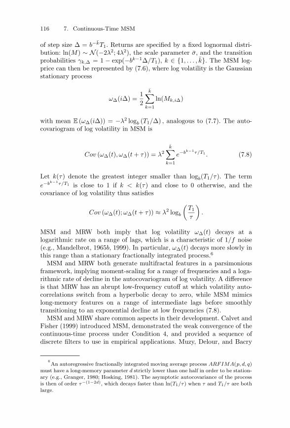
116 7. Continuous-Time MSM

of step size Δ = b−kT1. Returns are specified by a fixed lognormal distri-bution: ln(M) ∼ N (−2λ2; 4λ2), the scale parameter σ, and the transitionprobabilities γk,Δ = 1 − exp(−bk−1Δ/T1), k ∈ {1, . . . , k}. The MSM log-price can then be represented by (7.6), where log volatility is the Gaussianstationary process

ωΔ(iΔ) =12

k∑

k=1

ln(Mk,iΔ)

with mean E (ωΔ(iΔ)) = −λ2 logb (T1/Δ) , analogous to (7.7). The auto-covariogram of log volatility in MSM is

Cov (ωΔ(t), ωΔ(t + τ)) = λ2k∑

k=1

e−bk−1τ/T1 . (7.8)

Let k(τ) denote the greatest integer smaller than logb(T1/τ). The terme−bk−1τ/T1 is close to 1 if k < k(τ) and close to 0 otherwise, and thecovariance of log volatility thus satisfies

Cov (ωΔ(t);ωΔ(t + τ)) ≈ λ2 logb

(T1

τ

).

MSM and MRW both imply that log volatility ωΔ(t) decays at alogarithmic rate on a range of lags, which is a characteristic of 1/f noise(e.g., Mandelbrot, 1965b, 1999). In particular, ωΔ(t) decays more slowly inthis range than a stationary fractionally integrated process.6

MSM and MRW both generate multifractal features in a parsimoniousframework, implying moment-scaling for a range of frequencies and a loga-rithmic rate of decline in the autocovariogram of log volatility. A differenceis that MRW has an abrupt low-frequency cutoff at which volatility auto-correlations switch from a hyperbolic decay to zero, while MSM mimicslong-memory features on a range of intermediate lags before smoothlytransitioning to an exponential decline at low frequencies (7.8).

MSM and MRW share common aspects in their development. Calvet andFisher (1999) introduced MSM, demonstrated the weak convergence of thecontinuous-time process under Condition 4, and provided a sequence ofdiscrete filters to use in empirical applications. Muzy, Delour, and Bacry

6An autoregressive fractionally integrated moving average process ARFIMA(p, d, q)

must have a long-memory parameter d strictly lower than one half in order to be station-ary (e.g., Granger, 1980; Hosking, 1981). The asymptotic autocovariance of the processis then of order τ−(1−2d), which decays faster than ln(T1/τ) when τ and T1/τ are bothlarge.

7.4 Connection with Related Work 117

(2000) introduced MRW, and Bacry and Muzy (2003) used Condition 4to demonstrate the existence of a weak limit for their process. Calvet andFisher (2002b, 2004) and Calvet, Fisher, and Thompson (2006) demon-strated the use of econometric techniques such as maximum likelihoodestimation, simulated method of moments estimation, particle filtering,and closed-form multistep forecasting. In a similar vein to Calvet andFisher (2002b, 2004), Bacry, Kozhemyak, and Muzy (2008) show that MRWoutperforms standard GARCH-type specifications out-of-sample, whichconfirms the findings of Chapter 3 and Lux (2008).

MRW and a related approach by Barral and Mandelbrot (2002) incor-porate a continuum of time scales and do not require a “dilation param-eter” b, which provides elegance to the mathematical construct. In theseapproaches, trading time can be represented as an integral over a cone in thespace of scales and time.7 It remains an open question whether these math-ematical generalizations provide meaningful empirical differences comparedto MSM.

By contrast, MSM is based on Markov-switching and offers theadvantages of such models, including a closed-form likelihood function.8

Chapters 3 and 4 showed that in typical applications the MSM likeli-hood function levels off in the range of eight to ten volatility components,9

which suggests that improvements of the likelihood function are likely to belimited as k goes to infinity and the dilation parameter b correspondinglygoes to unity. The tractable Markov-switching state space representationalso aids the integration of MSM into asset pricing models, as will be seenin Part III.

The literature on multifractal volatility therefore continues to advanceon a number of fronts. While the methodologies used by researchers mayslightly differ, a salient common theme is that multifractal methods provideaccurate forecasts of volatility and estimates of value-at-risk. We anticipatethat these methods will continue to prove useful in financial applicationsin coming years.

Alternative stochastic volatility specifications

MSM and the multifractal processes discussed previously are stochas-tic volatility (SV) models that share certain moment-scaling properties.

7See the Appendix for further discussion.

8Calvet and Fisher (2002b) shows that the efficiency gains from ML estimation are

substantial relative to a variety of simulated method of moments estimators, and theimprovement in estimation efficiency confirmed by Lux (2008).

9Improvements in forecasting accuracy for MSM specifications with up to fifteen com-

ponents are found in Lux (2008). These results are obtained in a restricted setting wherethe dilation parameter b and lowest volatility component frequency γ1 are arbitrarilyfixed, due to difficulty identifying these parameters with method of moments estimation.In Chapter 3, we are able to estimate these parameters with reasonable precision usingthe likelihood function.

118 7. Continuous-Time MSM

Among the broader set of SV models, the long-memory stochastic volatil-ity (LMSV) models mentioned in Chapter 2 (e.g., Breidt, Crato, andde Lima, 1998; Comte and Renault, 1998; Harvey, 1998; Robinson andZaffaroni, 1998) have in common with multifractals slowly decliningautocovariograms of squared returns.

Recent developments in the LMSV literature have confirmed thatimprovements in volatility prediction can be obtained by models with long-memory features. Rohit Deo, Clifford Hurvich, and Yi Lu (2006) considera specification in which log volatility follows an autoregressive fractionallyintegrated moving average (ARFIMA) process:

Φ(L)(1 − L)dσ2t = Θ(L)ηt,

where L denotes the lag operator, ηt is IID N (0, σ2η), 0 < d < 0.5, and Φ

and Θ are polynomials with all roots outside the unit circle. The authorsestimate the model by maximizing the frequency domain quasi maximumlikelihood, derive an optimal multistep linear predictor, and show thatthis approach outperforms GARCH and component GARCH models10 athorizons of up to 4 weeks. These results confirm the potential benefits ofaccounting for low-frequency volatility fluctuations.

A related approach by Ole Barndorff-Nielsen and Neil Shephard (2001)specifies volatility as a weighted sum of independent Ornstein-Uhlenbeck(O-U) processes with heterogeneous persistence rates

σ2(t) =k∑

k=1

wkσ2k(t), (7.9)

where the weights wk are positive and sum to unity. Each process σ2k(t)

follows

d[σ2

k(t)]

= −λkσ2k(t)dt + dzk(λkt), (7.10)

where the {zk(t)} are independent non-Gaussian subordinators (that is,have nonnegative, independent and stationary increments).11 The compo-nents σ2

k therefore exhibit occasional upward jumps but otherwise revert

10Ding and Granger (1996) and Engle and Lee (1999) develop GARCH models with

multiple components. Empirical applications typically focus on the case of two volatilityfactors, representing long- and short-run fluctuations. Stochastic volatility specificationswith two components have also been shown to improve on single-factor specificationsunder a variety of in-sample diagnostics (Alizadeh, Brandt, and Diebold, 2002; Bates,2000; Bollerslev and Zhou, 2002; Chacko and Viceira, 2003; Chernov et al., 2003; Gallant,Hsu, and Tauchen, 1999; Xu and Taylor, 1994). Out-of-sample, a two-component volatil-ity model is useful for forecasting volatility at long horizons (Brandt and Jones, 2006),for option pricing (Christoffersen, Jacobs, and Wang, 2008), and for cross-sectional stockpricing (Adrian and Rosenberg, 2008).

11Bookstaber and Pomerantz (1989) consider a single-frequency version of the

Barndorff-Nielsen and Shephard model.

7.5 Discussion 119

toward zero at rate λk. An advantage of this approach is that closed-formexpressions are available for option pricing, as pursued by Nicolato andVenardos (2003).

Some of the features of the Barndorff-Nielsen and Shephard approachare similar to MSM. Volatility is hit by shocks of multiple durations, andthe autocorrelation function of returns is a sum of exponentials:

Corr(σ2(t);σ2(t + n)) =k∑

k=1

wke−λkn,

which can approximate a hyperbolic decay and mimic long memory,consistent with Proposition 1. Similar to MSM, the approach also has impli-cations for the power variation of returns, as discussed in Barndorff-Nielsenand Shephard (2003).

The O-U specification (7.10) implies the asymmetry that volatility com-ponents occasionally jump upward and otherwise slowly decline towardzero. In MSM, components remain constant until an arrival triggers thedraw of a new value, but as is the case with an O-U process, the conditionalexpectation of a future volatility state Et(Mk,t+n) = 1+ (1−γk)n(Mk,t−1)converges to the long-run mean.

As in other component SV models, the Barndorff-Nielsen specificationrequires a potentially large number of parameters as the dimensionality ofthe state space grows. This contrasts with the small number of parametersin MSM, obtained by imposing empirically verifiable restrictions acrossdifferent time scales. As is typical of other SV models, superposed Ornstein-Uhlenbeck volatility does not have a closed form likelihood, and inference istypically recommended to proceed by Monte Carlo Markov chain (MCMC)or other simulation-based methods. A unique characteristic of MSM amongSV models is that a large number of volatility components may be specifiedwith a small number of parameters, while also permitting a closed-formlikelihood function and convenient multistep forecasting.

7.5 Discussion

Continuous-time MSM is a multifrequency diffusion with fully stationaryincrements and heterogeneous volatility components, which can be natu-rally defined on an unbounded time domain. The instants of changes involatility components are randomly generated by a sequence of Poissonarrival processes with increasing frequencies. The model parsimoniouslycaptures the volatility persistence, moment-scaling, and thick tails thatcharacterize many financial time series, and is also consistent with the dif-ferent time scales of economic variables such as technology shocks, businessand earnings cycles, and liquidity shocks.

120 7. Continuous-Time MSM

MSM implies semimartingale prices and precludes arbitrage in a standardtwo-asset setting. Squared returns have long memory, and the highest finitemoment of returns may take any value greater than two. This wide rangeof tail behaviors is fully provided by intermittent bursts of volatility anddoes not require separate modeling of the tails. Forecasting is facilitated bydiscrete MSM which has a finite state space and a simple Markov structure.We show that the discretize model weakly converges to continuous-timeMSM as the grid step size goes to zero, ensuring that the discrete filtersare consistent in estimation and forecasting applications.

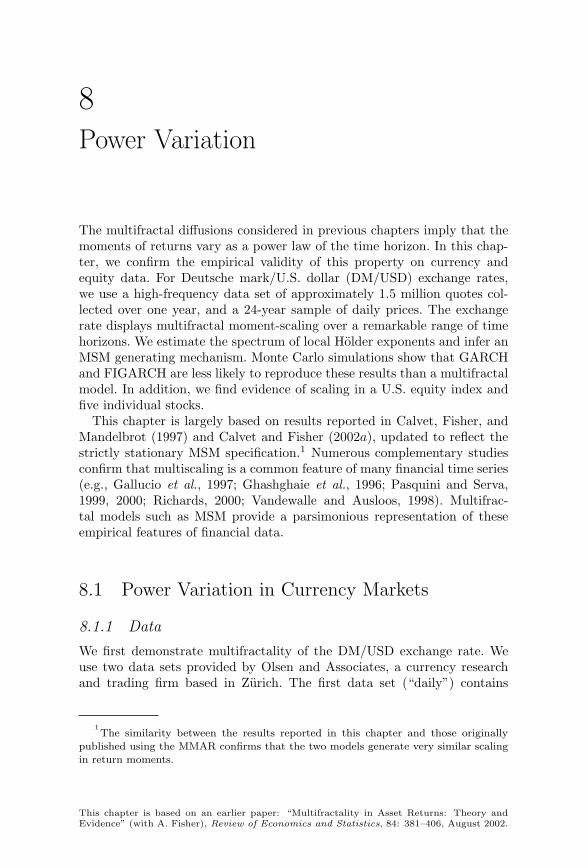
8Power Variation

The multifractal diffusions considered in previous chapters imply that themoments of returns vary as a power law of the time horizon. In this chap-ter, we confirm the empirical validity of this property on currency andequity data. For Deutsche mark/U.S. dollar (DM/USD) exchange rates,we use a high-frequency data set of approximately 1.5 million quotes col-lected over one year, and a 24-year sample of daily prices. The exchangerate displays multifractal moment-scaling over a remarkable range of timehorizons. We estimate the spectrum of local Holder exponents and infer anMSM generating mechanism. Monte Carlo simulations show that GARCHand FIGARCH are less likely to reproduce these results than a multifractalmodel. In addition, we find evidence of scaling in a U.S. equity index andfive individual stocks.

This chapter is largely based on results reported in Calvet, Fisher, andMandelbrot (1997) and Calvet and Fisher (2002a), updated to reflect thestrictly stationary MSM specification.1 Numerous complementary studiesconfirm that multiscaling is a common feature of many financial time series(e.g., Gallucio et al., 1997; Ghashghaie et al., 1996; Pasquini and Serva,1999, 2000; Richards, 2000; Vandewalle and Ausloos, 1998). Multifrac-tal models such as MSM provide a parsimonious representation of theseempirical features of financial data.

8.1 Power Variation in Currency Markets

8.1.1 DataWe first demonstrate multifractality of the DM/USD exchange rate. Weuse two data sets provided by Olsen and Associates, a currency researchand trading firm based in Zurich. The first data set (“daily”) contains

1The similarity between the results reported in this chapter and those originally

published using the MMAR confirms that the two models generate very similar scalingin return moments.

This chapter is based on an earlier paper: “Multifractality in Asset Returns: Theory andEvidence” (with A. Fisher), Review of Economics and Statistics, 84: 381–406, August 2002.

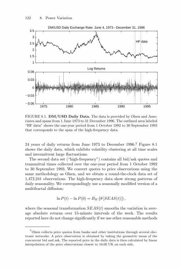
122 8. Power Variation

1

1.5

2

2.5

3

3.5DM/USD Daily Exchange Rate: June 4, 1973 – December 31, 1996

HF data

1975 1980 1985 1990 199520.06

20.03

0

0.03

0.06Log Returns

FIGURE 8.1. DM/USD Daily Data. The data is provided by Olsen and Asso-ciates and spans from 1 June 1973 to 31 December 1996. The outlined area labeled“HF data” shows the one-year period from 1 October 1992 to 30 September 1993that corresponds to the span of the high-frequency data.

24 years of daily returns from June 1973 to December 1996.2 Figure 8.1shows the daily data, which exhibits volatility clustering at all time scalesand intermittent large fluctuations.

The second data set (“high-frequency”) contains all bid/ask quotes andtransmittal times collected over the one-year period from 1 October 1992to 30 September 1993. We convert quotes to price observations using thesame methodology as Olsen, and we obtain a round-the-clock data set of1,472,241 observations. The high-frequency data show strong patterns ofdaily seasonality. We correspondingly use a seasonally modified version of amultifractal diffusion:

lnP (t) − lnP (0) = BH {θ [SEAS(t)]} ,

where the seasonal transformation SEAS(t) smooths the variation in aver-age absolute returns over 15-minute intervals of the week. The resultsreported here do not change significantly if we use other reasonable methods

2Olsen collects price quotes from banks and other institutions through several elec-

tronic networks. A price observation is obtained by taking the geometric mean of theconcurrent bid and ask. The reported price in the daily data is then calculated by linearinterpolation of the price observations closest to 16:00 UK on each side.

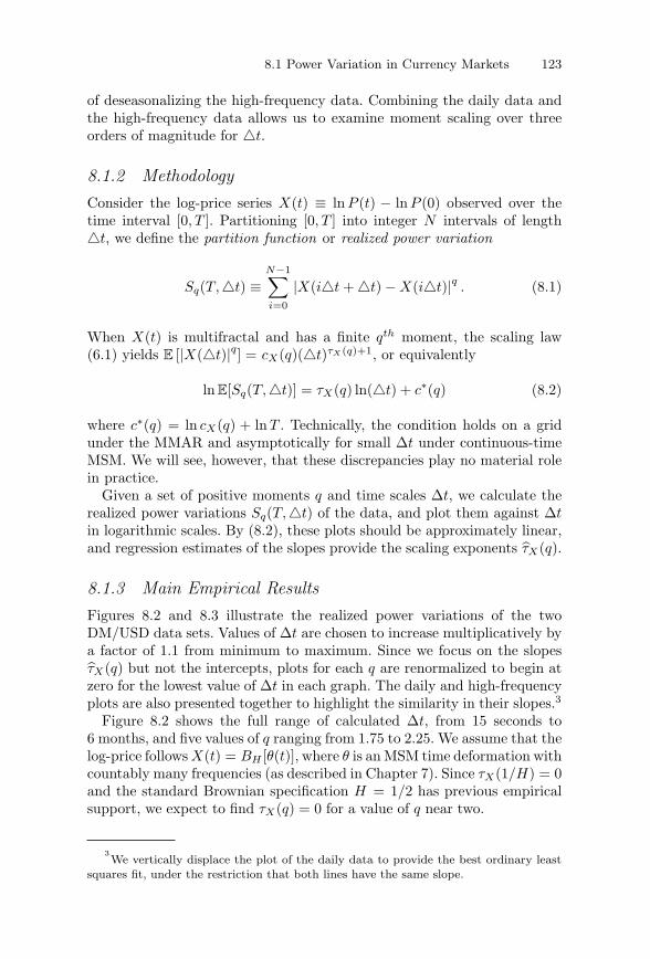
8.1 Power Variation in Currency Markets 123

of deseasonalizing the high-frequency data. Combining the daily data andthe high-frequency data allows us to examine moment scaling over threeorders of magnitude for �t.

8.1.2 MethodologyConsider the log-price series X(t) ≡ lnP (t) − lnP (0) observed over thetime interval [0, T ]. Partitioning [0, T ] into integer N intervals of length�t, we define the partition function or realized power variation

Sq(T, �t) ≡N−1∑

i=0

|X(i�t + �t) − X(i�t)|q . (8.1)

When X(t) is multifractal and has a finite qth moment, the scaling law(6.1) yields E [|X(�t)|q] = cX(q)(�t)τX(q)+1, or equivalently

ln E[Sq(T, �t)] = τX(q) ln(�t) + c∗(q) (8.2)

where c∗(q) = ln cX(q) + lnT . Technically, the condition holds on a gridunder the MMAR and asymptotically for small Δt under continuous-timeMSM. We will see, however, that these discrepancies play no material rolein practice.

Given a set of positive moments q and time scales Δt, we calculate therealized power variations Sq(T, �t) of the data, and plot them against Δtin logarithmic scales. By (8.2), these plots should be approximately linear,and regression estimates of the slopes provide the scaling exponents τX(q).

8.1.3 Main Empirical ResultsFigures 8.2 and 8.3 illustrate the realized power variations of the twoDM/USD data sets. Values of Δt are chosen to increase multiplicatively bya factor of 1.1 from minimum to maximum. Since we focus on the slopesτX(q) but not the intercepts, plots for each q are renormalized to begin atzero for the lowest value of Δt in each graph. The daily and high-frequencyplots are also presented together to highlight the similarity in their slopes.3

Figure 8.2 shows the full range of calculated Δt, from 15 seconds to6 months, and five values of q ranging from 1.75 to 2.25. We assume that thelog-price follows X(t) = BH [θ(t)], where θ is an MSM time deformation withcountably many frequencies (as described in Chapter 7). Since τX(1/H) = 0and the standard Brownian specification H = 1/2 has previous empiricalsupport, we expect to find τX(q) = 0 for a value of q near two.

3We vertically displace the plot of the daily data to provide the best ordinary least

squares fit, under the restriction that both lines have the same slope.

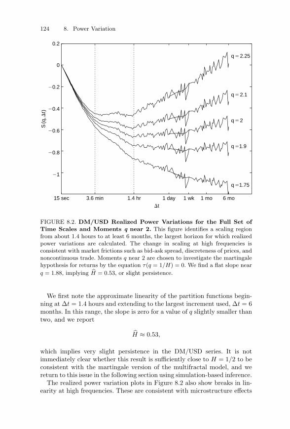
124 8. Power Variation

15 sec 3.6 min 1.4 hr 1 day 1 wk 1 mo 6 mo

0

20.2

20.4

20.6

20.8

21

0.2

Dt

S(q

,Dt)

q 51.75

q 51.9

q 5 2

q 5 2.1

q 5 2.25

FIGURE 8.2. DM/USD Realized Power Variations for the Full Set ofTime Scales and Moments q near 2. This figure identifies a scaling regionfrom about 1.4 hours to at least 6 months, the largest horizon for which realizedpower variations are calculated. The change in scaling at high frequencies isconsistent with market frictions such as bid-ask spread, discreteness of prices, andnoncontinuous trade. Moments q near 2 are chosen to investigate the martingalehypothesis for returns by the equation τ(q = 1/H) = 0. We find a flat slope nearq = 1.88, implying H = 0.53, or slight persistence.

We first note the approximate linearity of the partition functions begin-ning at Δt = 1.4 hours and extending to the largest increment used, Δt = 6months. In this range, the slope is zero for a value of q slightly smaller thantwo, and we report

H ≈ 0.53,

which implies very slight persistence in the DM/USD series. It is notimmediately clear whether this result is sufficiently close to H = 1/2 to beconsistent with the martingale version of the multifractal model, and wereturn to this issue in the following section using simulation-based inference.

The realized power variation plots in Figure 8.2 also show breaks in lin-earity at high frequencies. These are consistent with microstructure effects

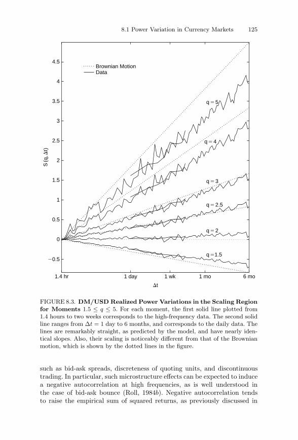
8.1 Power Variation in Currency Markets 125

1.4 hr 1 day 1 wk 1 mo 6 mo

0

0.5

20.5

1

1.5

2

2.5

3

3.5

4

4.5

Dt

S(q

,Dt)

q 51.5

q 5 2

q 5 2.5

q 5 3

q 5 4

q 5 5

Brownian MotionData

FIGURE 8.3. DM/USD Realized Power Variations in the Scaling Regionfor Moments 1.5 ≤ q ≤ 5. For each moment, the first solid line plotted from1.4 hours to two weeks corresponds to the high-frequency data. The second solidline ranges from Δt = 1 day to 6 months, and corresponds to the daily data. Thelines are remarkably straight, as predicted by the model, and have nearly iden-tical slopes. Also, their scaling is noticeably different from that of the Brownianmotion, which is shown by the dotted lines in the figure.

such as bid-ask spreads, discreteness of quoting units, and discontinuoustrading. In particular, such microstructure effects can be expected to inducea negative autocorrelation at high frequencies, as is well understood inthe case of bid-ask bounce (Roll, 1984b). Negative autocorrelation tendsto raise the empirical sum of squared returns, as previously discussed in

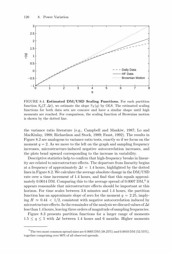
126 8. Power Variation

0 1 2 3 4 5 6 7 8

0

21

0.5

20.5

1

1.5

2

2.5

3

q

�(q

)

Brownian MotionHF DataDaily Data

FIGURE 8.4. Estimated DM/USD Scaling Functions. For each partitionfunction Sq(T, Δt), we estimate the slope τX(q) by OLS. The estimated scalingfunctions for both data sets are concave and have a similar shape until highmoments are reached. For comparison, the scaling function of Brownian motionis shown by the dotted line.

the variance ratio literature (e.g., Campbell and Mankiw, 1987; Lo andMacKinlay, 1988; Richardson and Stock, 1989; Faust, 1992). The results inFigure 8.2 are analogous to variance ratio tests, exactly so if we focus on themoment q = 2. As we move to the left on the graph and sampling frequencyincreases, microstructure-induced negative autocorrelation increases, andthe plots bend upward corresponding to the increase in variability.

Descriptive statistics help to confirm that high-frequency breaks in linear-ity are related to microstructure effects. The departure from linearity beginsat a frequency of approximately Δt = 1.4 hours, highlighted by the dottedlines in Figure 8.2. We calculate the average absolute change in the DM/USDrate over a time increment of 1.4 hours, and find that this equals approxi-mately 0.0014 DM. Comparing this to the average spread of 0.0007 DM,4 itappears reasonable that microstructure effects should be important at thishorizon. For time scales between 3.6 minutes and 1.4 hours, the partitionfunction has an approximate slope of zero for the moment q = 2.25, imply-ing H ≈ 0.44 < 1/2, consistent with negative autocorrelation induced bymicrostructure effects. In the remainder of the analysiswediscardvalues ofΔtless than 1.4 hours, leaving three orders ofmagnitude of sampling frequencies.

Figure 8.3 presents partition functions for a larger range of moments1.5 ≤ q ≤ 5 with Δt between 1.4 hours and 6 months. Higher moments

4The two most common spread sizes are 0.0005 DM (38.25%) and 0.0010 DM (52.55%),

together comprising over 90% of all observed spreads.

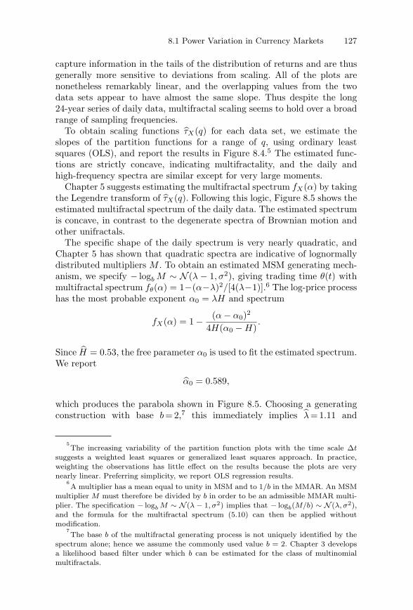
8.1 Power Variation in Currency Markets 127

capture information in the tails of the distribution of returns and are thusgenerally more sensitive to deviations from scaling. All of the plots arenonetheless remarkably linear, and the overlapping values from the twodata sets appear to have almost the same slope. Thus despite the long24-year series of daily data, multifractal scaling seems to hold over a broadrange of sampling frequencies.

To obtain scaling functions τX(q) for each data set, we estimate theslopes of the partition functions for a range of q, using ordinary leastsquares (OLS), and report the results in Figure 8.4.5 The estimated func-tions are strictly concave, indicating multifractality, and the daily andhigh-frequency spectra are similar except for very large moments.

Chapter 5 suggests estimating the multifractal spectrum fX(α) by takingthe Legendre transform of τX(q). Following this logic, Figure 8.5 shows theestimated multifractal spectrum of the daily data. The estimated spectrumis concave, in contrast to the degenerate spectra of Brownian motion andother unifractals.

The specific shape of the daily spectrum is very nearly quadratic, andChapter 5 has shown that quadratic spectra are indicative of lognormallydistributed multipliers M . To obtain an estimated MSM generating mech-anism, we specify − logb M ∼ N (λ − 1, σ2), giving trading time θ(t) withmultifractal spectrum fθ(α) = 1−(α−λ)2/[4(λ−1)].6 The log-price processhas the most probable exponent α0 = λH and spectrum

fX(α) = 1 − (α − α0)2

4H(α0 − H).

Since H = 0.53, the free parameter α0 is used to fit the estimated spectrum.We report

α0 = 0.589,

which produces the parabola shown in Figure 8.5. Choosing a generatingconstruction with base b = 2,7 this immediately implies λ = 1.11 and

5The increasing variability of the partition function plots with the time scale Δt

suggests a weighted least squares or generalized least squares approach. In practice,weighting the observations has little effect on the results because the plots are verynearly linear. Preferring simplicity, we report OLS regression results.

6A multiplier has a mean equal to unity in MSM and to 1/b in the MMAR. An MSM

multiplier M must therefore be divided by b in order to be an admissible MMAR multi-plier. The specification − logb M ∼ N (λ − 1, σ2) implies that − logb(M/b) ∼ N (λ, σ2),and the formula for the multifractal spectrum (5.10) can then be applied withoutmodification.

7The base b of the multifractal generating process is not uniquely identified by the

spectrum alone; hence we assume the commonly used value b = 2. Chapter 3 developsa likelihood based filter under which b can be estimated for the class of multinomialmultifractals.

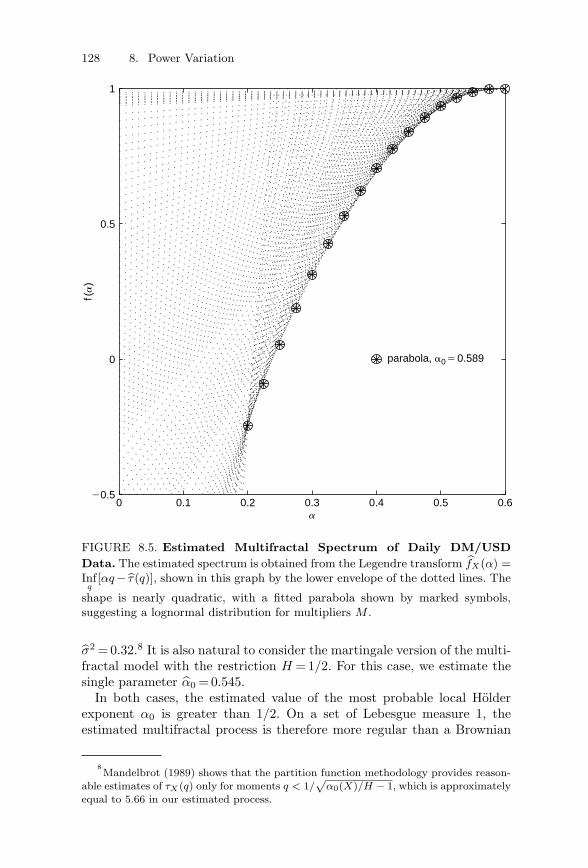
128 8. Power Variation

0 0.1 0.2 0.3 0.4 0.5 0.6

0

0.5

20.5

1f(

�)

parabola, a05 0.589

�

FIGURE 8.5. Estimated Multifractal Spectrum of Daily DM/USDData. The estimated spectrum is obtained from the Legendre transform fX(α) =Inf

q[αq − τ(q)], shown in this graph by the lower envelope of the dotted lines. The

shape is nearly quadratic, with a fitted parabola shown by marked symbols,suggesting a lognormal distribution for multipliers M .

σ2 = 0.32.8 It is also natural to consider the martingale version of the multi-fractal model with the restriction H = 1/2. For this case, we estimate thesingle parameter α0 = 0.545.

In both cases, the estimated value of the most probable local Holderexponent α0 is greater than 1/2. On a set of Lebesgue measure 1, theestimated multifractal process is therefore more regular than a Brownian

8Mandelbrot (1989) shows that the partition function methodology provides reason-

able estimates of τX(q) only for moments q < 1/√

α0(X)/H − 1, which is approximatelyequal to 5.66 in our estimated process.

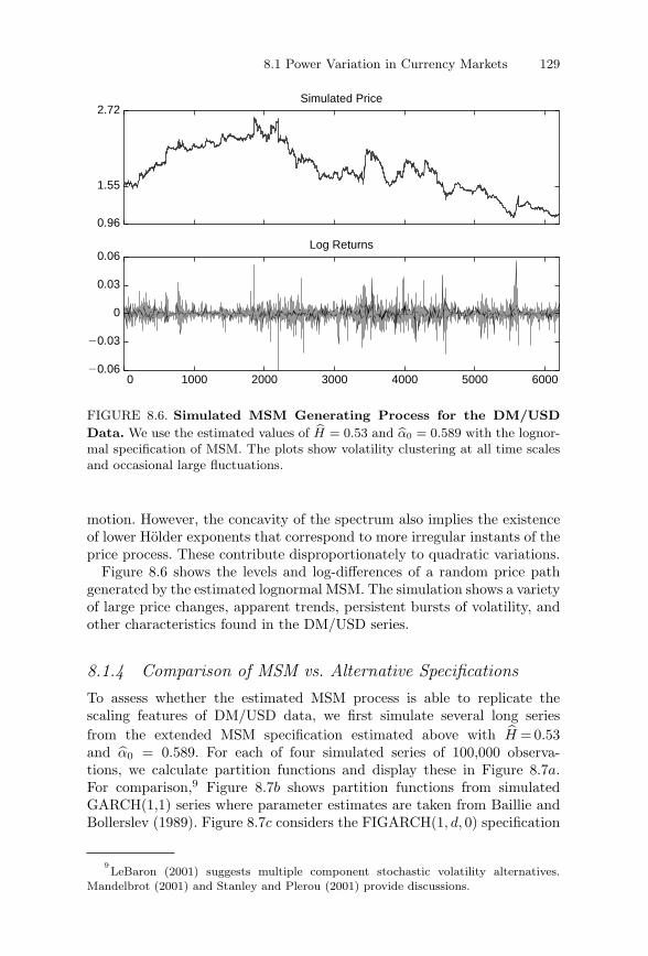
8.1 Power Variation in Currency Markets 129

0.96

1.55

2.72Simulated Price

0 1000 2000 3000 4000 5000 600020.06

20.03

0

0.03

0.06Log Returns

FIGURE 8.6. Simulated MSM Generating Process for the DM/USDData. We use the estimated values of H = 0.53 and α0 = 0.589 with the lognor-mal specification of MSM. The plots show volatility clustering at all time scalesand occasional large fluctuations.

motion. However, the concavity of the spectrum also implies the existenceof lower Holder exponents that correspond to more irregular instants of theprice process. These contribute disproportionately to quadratic variations.

Figure 8.6 shows the levels and log-differences of a random price pathgenerated by the estimated lognormal MSM. The simulation shows a varietyof large price changes, apparent trends, persistent bursts of volatility, andother characteristics found in the DM/USD series.

8.1.4 Comparison of MSM vs. Alternative SpecificationsTo assess whether the estimated MSM process is able to replicate thescaling features of DM/USD data, we first simulate several long seriesfrom the extended MSM specification estimated above with H = 0.53and α0 = 0.589. For each of four simulated series of 100,000 observa-tions, we calculate partition functions and display these in Figure 8.7a.For comparison,9 Figure 8.7b shows partition functions from simulatedGARCH(1,1) series where parameter estimates are taken from Baillie andBollerslev (1989). Figure 8.7c considers the FIGARCH(1, d, 0) specification

9LeBaron (2001) suggests multiple component stochastic volatility alternatives.

Mandelbrot (2001) and Stanley and Plerou (2001) provide discussions.

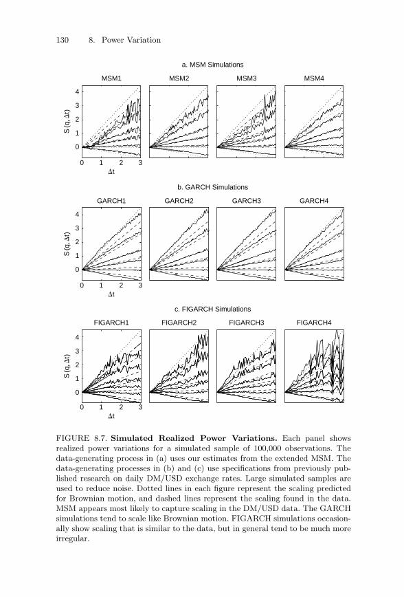
130 8. Power Variation

0 1 2 3

0

1

2

3

4

Dt

S(q

,Dt)

MSM1 MSM2 MSM3 MSM4

a. MSM SimulationsS

(q,D

t)

0 1 2 3

0

1

2

3

4

Dt

GARCH4GARCH1 GARCH2 GARCH3

b. GARCH Simulations

S(q

,Dt)

0 1 2 3

0

1

2

3

4

Dt

FIGARCH1 FIGARCH2 FIGARCH3 FIGARCH4

c. FIGARCH Simulations

FIGURE 8.7. Simulated Realized Power Variations. Each panel showsrealized power variations for a simulated sample of 100,000 observations. Thedata-generating process in (a) uses our estimates from the extended MSM. Thedata-generating processes in (b) and (c) use specifications from previously pub-lished research on daily DM/USD exchange rates. Large simulated samples areused to reduce noise. Dotted lines in each figure represent the scaling predictedfor Brownian motion, and dashed lines represent the scaling found in the data.MSM appears most likely to capture scaling in the DM/USD data. The GARCHsimulations tend to scale like Brownian motion. FIGARCH simulations occasion-ally show scaling that is similar to the data, but in general tend to be much moreirregular.

8.1 Power Variation in Currency Markets 131

of Baillie, Bollerslev, and Mikkelsen (1996). The figure shows that theMSM partition functions are approximately linear and close to the slopesof the DM/USD data. By contrast, the GARCH(1, 1) partition functionsare fairly linear, but their apparent slope is similar to the predicted slopeof Brownian motion rather than the data. This is symptomatic of shortmemory in GARCH models. Over long time periods, temporal clusteringdisappears, and GARCH scales like a Brownian motion. The FIGARCHpartition function plots appear more irregular than those of MSM and thedata.

We now provide a more systematic assessment of ability to replicate thescaling features of DM/USD data. The analysis focuses on four processes:the extended MSM (with arbitrary H), the martingale MSM (H = 1/2),FIGARCH, and GARCH. These models are, respectively, indexed by m ∈{1, . . . , 4}. For each model m, we simulate J = 10,000 paths with thesame length T = 6,118 as the DM/USD data. We denote each path byY m

j = {Y mj,t}T

t=1, (1 ≤ j ≤ J), and we focus the analysis on the moments q ∈Q= {0.5, 1, 2, 3, 5}. For each path and each q, an OLS regression providesa slope estimate τ(q, Y m

j ) and the corresponding sum of squared errorsSSE(q, Y m

j ). Tables 8.1 and 8.2 report the percentiles of these statistics foreach model. The distributions of the reported statistics appear unimodal,with smoothly declining tails.

Table 8.1 shows that the extended MSM is very close to the data in bothits theoretically predicted slopes τ0 and the mean slopes τ . Furthermore, theestimated slopes from the DM/USD data are well within the central bells ofthe simulated slope distributions generated by the extended MSM. For themartingale version of MSM, the estimated slopes from the DM/USD dataare generally close to the model slopes, but for low moments the statisticsfrom the data are in the upper tail of the simulated distribution for themodel.

Table 8.2 analyzes the variability of the simulated partition functionsaround their slopes. The extended and martingale versions of the MSMyield nearly identical results. For low moments, the data falls well withinthe likely range of the SSE statistic for both models. For high moments,the partition functions are typically more variable for the simulated MSMthan for the data. Overall, MSM appears to successfully match the mainscaling features of the data.

Comparing GARCH and FIGARCH to these results, Tables 8.1 and 8.2confirm that the GARCH partition functions, while linear, have very dif-ferent slopes than the DM/USD data. The simulated FIGARCH slopesimprove over the GARCH slopes, but are not as close to the data as themultifractal model. The SSEs from the data, reported in Table 8.2, are alsofar in the tails of their distributions generated under FIGARCH. Thus, thetwo MSM specifications appear more likely to replicate the scaling featuresof the exchange rate data than alternative models.

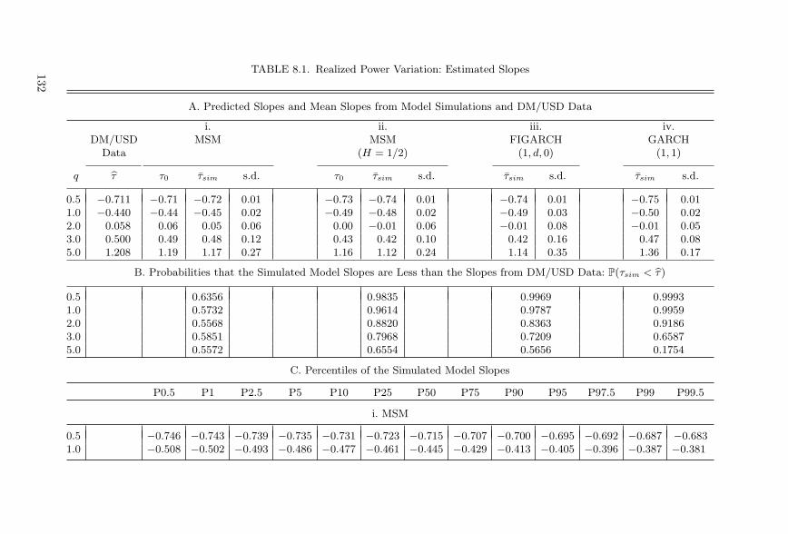
TABLE 8.1. Realized Power Variation: Estimated Slopes

A. Predicted Slopes and Mean Slopes from Model Simulations and DM/USD Data

i. ii. iii. iv.DM/USD MSM MSM FIGARCH GARCH

Data (H = 1/2) (1, d, 0) (1, 1)

q τ τ0 τsim s.d. τ0 τsim s.d. τsim s.d. τsim s.d.

0.5 −0.711 −0.71 −0.72 0.01 −0.73 −0.74 0.01 −0.74 0.01 −0.75 0.011.0 −0.440 −0.44 −0.45 0.02 −0.49 −0.48 0.02 −0.49 0.03 −0.50 0.022.0 0.058 0.06 0.05 0.06 0.00 −0.01 0.06 −0.01 0.08 −0.01 0.053.0 0.500 0.49 0.48 0.12 0.43 0.42 0.10 0.42 0.16 0.47 0.085.0 1.208 1.19 1.17 0.27 1.16 1.12 0.24 1.14 0.35 1.36 0.17

B. Probabilities that the Simulated Model Slopes are Less than the Slopes from DM/USD Data: P(τsim < τ)

0.5 0.6356 0.9835 0.9969 0.99931.0 0.5732 0.9614 0.9787 0.99592.0 0.5568 0.8820 0.8363 0.91863.0 0.5851 0.7968 0.7209 0.65875.0 0.5572 0.6554 0.5656 0.1754

C. Percentiles of the Simulated Model Slopes

P0.5 P1 P2.5 P5 P10 P25 P50 P75 P90 P95 P97.5 P99 P99.5

i. MSM

0.5 −0.746 −0.743 −0.739 −0.735 −0.731 −0.723 −0.715 −0.707 −0.700 −0.695 −0.692 −0.687 −0.6831.0 −0.508 −0.502 −0.493 −0.486 −0.477 −0.461 −0.445 −0.429 −0.413 −0.405 −0.396 −0.387 −0.381

132

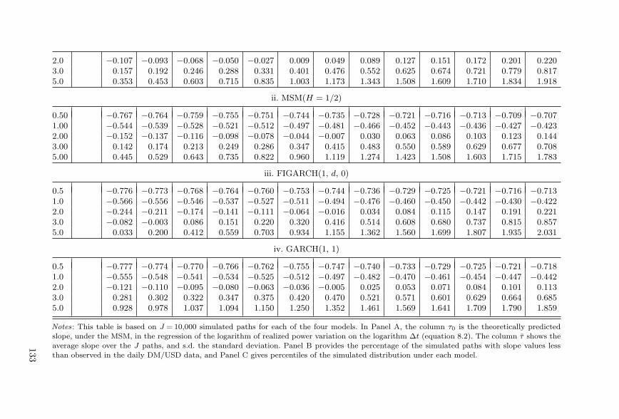
2.0 −0.107 −0.093 −0.068 −0.050 −0.027 0.009 0.049 0.089 0.127 0.151 0.172 0.201 0.2203.0 0.157 0.192 0.246 0.288 0.331 0.401 0.476 0.552 0.625 0.674 0.721 0.779 0.8175.0 0.353 0.453 0.603 0.715 0.835 1.003 1.173 1.343 1.508 1.609 1.710 1.834 1.918

ii. MSM(H = 1/2)

0.50 −0.767 −0.764 −0.759 −0.755 −0.751 −0.744 −0.735 −0.728 −0.721 −0.716 −0.713 −0.709 −0.7071.00 −0.544 −0.539 −0.528 −0.521 −0.512 −0.497 −0.481 −0.466 −0.452 −0.443 −0.436 −0.427 −0.4232.00 −0.152 −0.137 −0.116 −0.098 −0.078 −0.044 −0.007 0.030 0.063 0.086 0.103 0.123 0.1443.00 0.142 0.174 0.213 0.249 0.286 0.347 0.415 0.483 0.550 0.589 0.629 0.677 0.7085.00 0.445 0.529 0.643 0.735 0.822 0.960 1.119 1.274 1.423 1.508 1.603 1.715 1.783

iii. FIGARCH(1, d, 0)

0.5 −0.776 −0.773 −0.768 −0.764 −0.760 −0.753 −0.744 −0.736 −0.729 −0.725 −0.721 −0.716 −0.7131.0 −0.566 −0.556 −0.546 −0.537 −0.527 −0.511 −0.494 −0.476 −0.460 −0.450 −0.442 −0.430 −0.4222.0 −0.244 −0.211 −0.174 −0.141 −0.111 −0.064 −0.016 0.034 0.084 0.115 0.147 0.191 0.2213.0 −0.082 −0.003 0.086 0.151 0.220 0.320 0.416 0.514 0.608 0.680 0.737 0.815 0.8575.0 0.033 0.200 0.412 0.559 0.703 0.934 1.155 1.362 1.560 1.699 1.807 1.935 2.031

iv. GARCH(1, 1)

0.5 −0.777 −0.774 −0.770 −0.766 −0.762 −0.755 −0.747 −0.740 −0.733 −0.729 −0.725 −0.721 −0.7181.0 −0.555 −0.548 −0.541 −0.534 −0.525 −0.512 −0.497 −0.482 −0.470 −0.461 −0.454 −0.447 −0.4422.0 −0.121 −0.110 −0.095 −0.080 −0.063 −0.036 −0.005 0.025 0.053 0.071 0.084 0.101 0.1133.0 0.281 0.302 0.322 0.347 0.375 0.420 0.470 0.521 0.571 0.601 0.629 0.664 0.6855.0 0.928 0.978 1.037 1.094 1.150 1.250 1.352 1.461 1.569 1.641 1.709 1.790 1.859

Notes: This table is based on J = 10,000 simulated paths for each of the four models. In Panel A, the column τ0 is the theoretically predictedslope, under the MSM, in the regression of the logarithm of realized power variation on the logarithm Δt (equation 8.2). The column τ shows theaverage slope over the J paths, and s.d. the standard deviation. Panel B provides the percentage of the simulated paths with slope values lessthan observed in the daily DM/USD data, and Panel C gives percentiles of the simulated distribution under each model.

133

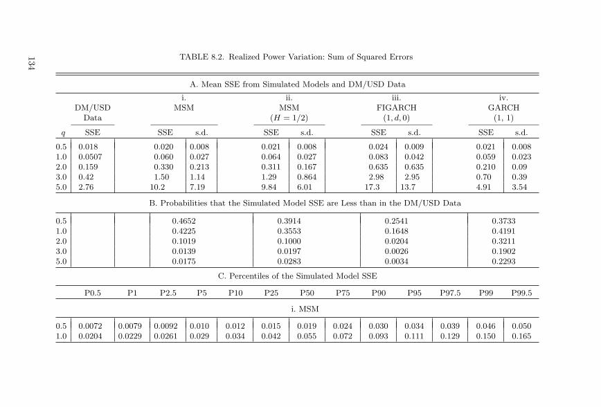
TABLE 8.2. Realized Power Variation: Sum of Squared Errors

A. Mean SSE from Simulated Models and DM/USD Data

i. ii. iii. iv.DM/USD MSM MSM FIGARCH GARCH

Data (H = 1/2) (1, d, 0) (1, 1)

q SSE SSE s.d. SSE s.d. SSE s.d. SSE s.d.

0.5 0.018 0.020 0.008 0.021 0.008 0.024 0.009 0.021 0.0081.0 0.0507 0.060 0.027 0.064 0.027 0.083 0.042 0.059 0.0232.0 0.159 0.330 0.213 0.311 0.167 0.635 0.635 0.210 0.093.0 0.42 1.50 1.14 1.29 0.864 2.98 2.95 0.70 0.395.0 2.76 10.2 7.19 9.84 6.01 17.3 13.7 4.91 3.54

B. Probabilities that the Simulated Model SSE are Less than in the DM/USD Data

0.5 0.4652 0.3914 0.2541 0.37331.0 0.4225 0.3553 0.1648 0.41912.0 0.1019 0.1000 0.0204 0.32113.0 0.0139 0.0197 0.0026 0.19025.0 0.0175 0.0283 0.0034 0.2293

C. Percentiles of the Simulated Model SSE

P0.5 P1 P2.5 P5 P10 P25 P50 P75 P90 P95 P97.5 P99 P99.5

i. MSM

0.5 0.0072 0.0079 0.0092 0.010 0.012 0.015 0.019 0.024 0.030 0.034 0.039 0.046 0.0501.0 0.0204 0.0229 0.0261 0.029 0.034 0.042 0.055 0.072 0.093 0.111 0.129 0.150 0.165

134

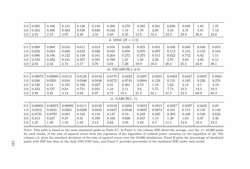
2.0 0.095 0.106 0.121 0.136 0.158 0.206 0.279 0.395 0.561 0.698 0.849 1.05 1.273.0 0.352 0.396 0.462 0.530 0.630 0.842 1.18 1.78 2.69 3.44 4.31 5.81 7.125.0 2.25 2.52 2.97 3.46 4.16 5.68 8.25 12.5 18.4 23.2 28.9 36.8 42.8

ii. MSM (H = 1/2)

0.5 0.008 0.008 0.010 0.011 0.013 0.016 0.020 0.025 0.031 0.036 0.040 0.048 0.0531.0 0.022 0.024 0.028 0.032 0.036 0.045 0.058 0.076 0.097 0.113 0.131 0.155 0.1842.0 0.096 0.106 0.122 0.138 0.161 0.204 0.272 0.375 0.511 0.622 0.752 0.92 1.113.0 0.333 0.382 0.441 0.507 0.591 0.768 1.07 1.58 2.26 2.87 3.63 4.93 6.115.0 2.04 2.34 2.74 3.17 3.76 5.04 7.26 10.9 16.3 20.4 25.5 33.8 38.1

iii. FIGARCH(1, d, 0)

0.5 0.00873 0.00969 0.0112 0.0126 0.0144 0.0179 0.0229 0.0287 0.0355 0.0403 0.0447 0.0507 0.05611.0 0.026 0.0291 0.034 0.0386 0.0448 0.0572 0.0745 0.0984 0.129 0.155 0.185 0.228 0.2762.0 0.126 0.14 0.165 0.192 0.227 0.31 0.461 0.73 1.18 1.62 2.14 3.1 4.183.0 0.453 0.527 0.64 0.751 0.931 1.34 2.11 3.6 5.75 7.74 10.3 14.3 19.45.0 2.99 3.42 4.13 4.94 6.07 8.73 13.5 21.4 32.1 41.5 52.4 68.9 85.3

iv. GARCH(1, 1)

0.5 0.00804 0.00872 0.00995 0.0111 0.0128 0.0159 0.0202 0.0254 0.0315 0.0357 0.0397 0.0455 0.051.0 0.0212 0.0232 0.0265 0.0299 0.0343 0.0427 0.0546 0.0697 0.0874 0.101 0.115 0.135 0.1492.0 0.0725 0.0793 0.091 0.103 0.116 0.147 0.19 0.249 0.325 0.383 0.449 0.548 0.6243.0 0.214 0.237 0.27 0.31 0.356 0.456 0.608 0.827 1.13 1.39 1.64 2.07 2.465.0 1.25 1.39 1.59 1.83 2.14 2.84 3.95 5.83 8.5 11.1 13.9 18.4 23.2

Notes: This table is based on the same simulated paths as Table 8.1. In Panel A, the column SSE shows the average, over the J =10,000 pathsfor each model, of the sum of squared errors from the regression of the logarithm of realized power variation on the logarithm of Δt. Thecolumn s.d. gives the standard deviation of the sum of squared errors over the 10,000 simulations. Panel B gives the percentage of simulatedpaths with SSE less than in the daily DM/USD data, and Panel C provides percentiles of the simulated SSE under each model.

135

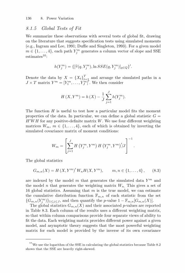
136 8. Power Variation

8.1.5 Global Tests of FitWe summarize these observations with several tests of global fit, drawingon the literature that suggests specification tests using simulated moments(e.g., Ingram and Lee, 1991; Duffie and Singleton, 1993). For a given modelm ∈ {1, . . . , 4}, each path Y m

j generates a column vector of slope and SSEestimates10:

h(Y mj ) = {[τ(q, Y m

j ), lnSSE(q, Y mj )]q∈Q}′.

Denote the data by X = {Xt}Tt=1 and arrange the simulated paths in a

J × T matrix Y m = [Y m1 , . . . , Y m

J ]′. We then consider

H (X, Y m) = h (X) − 1J

J∑

j=1

h(Y mj ).

The function H is useful to test how a particular model fits the momentproperties of the data. In particular, we can define a global statistic G =H ′WH for any positive-definite matrix W . We use four different weightingmatrices Wm, m ∈ {1, . . . , 4}, each of which is obtained by inverting thesimulated covariance matrix of moment conditions:

Wm =

⎡

⎣J∑

j=1

H(Y m

j , Y m)H

(Y m

j , Y m)′/J

⎤

⎦−1

.

The global statistics

Gm,n(X) = H (X, Y m)′WnH(X, Y m), m, n ∈ {1, . . . , 4} , (8.3)

are indexed by the model m that generates the simulated data Y m andthe model n that generates the weighting matrix Wn. This gives a set of16 global statistics. Assuming that m is the true model, we can estimatethe cumulative distribution function Fm,n of each statistic from the set{Gm,n(Y m

j )}1≤j≤J , and then quantify the p-value 1 − Fm,n[Gm,n(X)].The global statistics Gm,n(X) and their associated p-values are reported

in Table 8.3. Each column of the results uses a different weighting matrix,so that within column comparisons provide four separate views of ability tofit the data. Each weighting matrix provides different power against a givenmodel, and asymptotic theory suggests that the most powerful weightingmatrix for each model is provided by the inverse of its own covariance

10We use the logarithm of the SSE in calculating the global statistics because Table 8.2

shows that the SSE are heavily right-skewed.

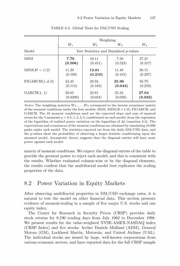
8.2 Power Variation in Equity Markets 137

TABLE 8.3. Global Tests for DM/USD Scaling

WeightingW1 W2 W3 W4

Model Test Statistics and Simulated p-values

MSM 7.70 10.11 7.50 27.21(0.506) (0.451) (0.523) (0.317)

MSM(H = 1/2) 11.29 12.81 11.49 20.15(0.199) (0.210) (0.185) (0.297)

FIGARCH(1, d, 0) 24.45 28.94 25.96 58.79(0.114) (0.163) (0.043) (0.259)

GARCH(1, 1) 20.65 22.81 25.34 27.04(0.0290) (0.024) (0.030) (0.032)

Notes: The weighting matrices W1, . . . , W4 correspond to the inverse covariance matrixof the moment conditions under the four models: MSM, MSM(H =1/2), FIGARCH, andGARCH. The 10 moment conditions used are the expected slope and sum of squarederrors for the 5 moments q = 0.5, 1, 2, 3, 5, conditioned on each model, from the regressionof the logarithm of realized power variation on the logarithm of Δt (equation 8.2). Theexpectations and covariances of the moment conditions are obtained by simulating 10,000paths under each model. The statistics reported are from the daily DM/USD data, andthe p-values show the probability of observing a larger statistic conditioning upon theassumed model. Asymptotic theory suggests that the diagonal entries will have mostpower against each model.

matrix of moment conditions. We expect the diagonal entries of the table toprovide the greatest power to reject each model, and this is consistent withthe results. Whether evaluated column-wise or by the diagonal elements,the results confirm that the multifractal model best replicates the scalingproperties of the data.

8.2 Power Variation in Equity Markets

After observing multifractal properties in DM/USD exchange rates, it isnatural to test the model on other financial data. This section presentsevidence of moment-scaling in a sample of five major U.S. stocks and oneequity index.

The Center for Research in Security Prices (CRSP) provides dailystock returns for 9,190 trading days from July 1962 to December 1998.We present results for the value-weighted NYSE-AMEX-NASDAQ index(CRSP Index) and five stocks: Archer Daniels Midland (ADM), GeneralMotors (GM), Lockheed Martin, Motorola, and United Airlines (UAL).The individual stocks are issued by large, well-known corporations fromvarious economic sectors, and have reported data for the full CRSP sample

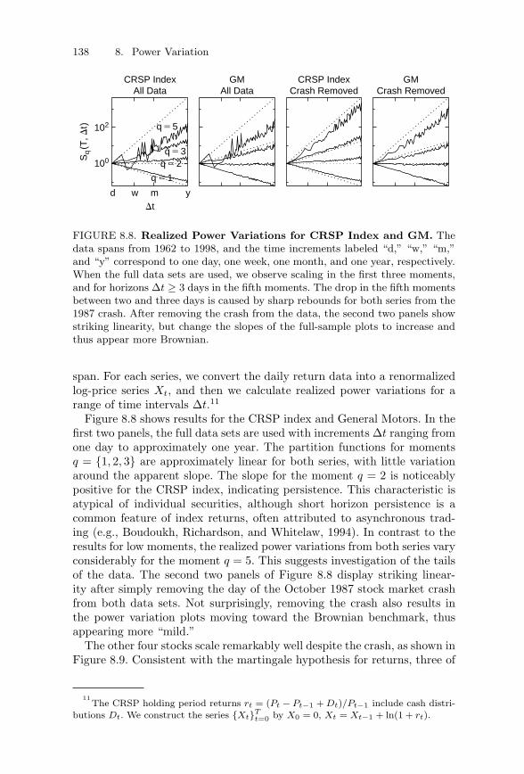
138 8. Power Variation

d w m y

100

102

CRSP IndexAll Data

Sq(T

, Dt)

q 5 1

q 5 2q 5 3

q 5 5

GMAll Data

CRSP IndexCrash Removed

GMCrash Removed

Dt

FIGURE 8.8. Realized Power Variations for CRSP Index and GM. Thedata spans from 1962 to 1998, and the time increments labeled “d,” “w,” “m,”and “y” correspond to one day, one week, one month, and one year, respectively.When the full data sets are used, we observe scaling in the first three moments,and for horizons Δt ≥ 3 days in the fifth moments. The drop in the fifth momentsbetween two and three days is caused by sharp rebounds for both series from the1987 crash. After removing the crash from the data, the second two panels showstriking linearity, but change the slopes of the full-sample plots to increase andthus appear more Brownian.

span. For each series, we convert the daily return data into a renormalizedlog-price series Xt, and then we calculate realized power variations for arange of time intervals Δt.11

Figure 8.8 shows results for the CRSP index and General Motors. In thefirst two panels, the full data sets are used with increments Δt ranging fromone day to approximately one year. The partition functions for momentsq = {1, 2, 3} are approximately linear for both series, with little variationaround the apparent slope. The slope for the moment q = 2 is noticeablypositive for the CRSP index, indicating persistence. This characteristic isatypical of individual securities, although short horizon persistence is acommon feature of index returns, often attributed to asynchronous trad-ing (e.g., Boudoukh, Richardson, and Whitelaw, 1994). In contrast to theresults for low moments, the realized power variations from both series varyconsiderably for the moment q = 5. This suggests investigation of the tailsof the data. The second two panels of Figure 8.8 display striking linear-ity after simply removing the day of the October 1987 stock market crashfrom both data sets. Not surprisingly, removing the crash also results inthe power variation plots moving toward the Brownian benchmark, thusappearing more “mild.”

The other four stocks scale remarkably well despite the crash, as shown inFigure 8.9. Consistent with the martingale hypothesis for returns, three of

11The CRSP holding period returns rt = (Pt − Pt−1 + Dt)/Pt−1 include cash distri-

butions Dt. We construct the series {Xt}Tt=0 by X0 = 0, Xt = Xt−1 + ln(1 + rt).

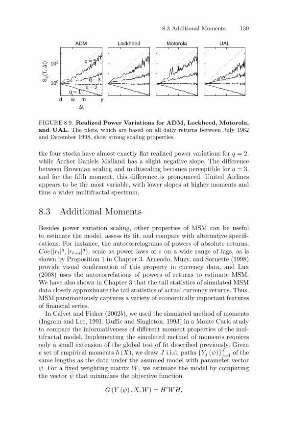
8.3 Additional Moments 139

ADM

q 5 1q 5 2

q 5 3

q 5 5

Lockheed Motorola UAL

d w m y

100

102

Sq(T

, Dt)

Dt

FIGURE 8.9. Realized Power Variations for ADM, Lockheed, Motorola,and UAL. The plots, which are based on all daily returns between July 1962and December 1998, show strong scaling properties.

the four stocks have almost exactly flat realized power variations for q = 2,while Archer Daniels Midland has a slight negative slope. The differencebetween Brownian scaling and multiscaling becomes perceptible for q = 3,and for the fifth moment, this difference is pronounced. United Airlinesappears to be the most variable, with lower slopes at higher moments andthus a wider multifractal spectrum.

8.3 Additional Moments

Besides power variation scaling, other properties of MSM can be usefulto estimate the model, assess its fit, and compare with alternative specifi-cations. For instance, the autocorrelograms of powers of absolute returns,Cov(|rt|q, |rt+s|q), scale as power laws of s on a wide range of lags, as isshown by Proposition 1 in Chapter 3. Arneodo, Muzy, and Sornette (1998)provide visual confirmation of this property in currency data, and Lux(2008) uses the autocorrelations of powers of returns to estimate MSM.We have also shown in Chapter 3 that the tail statistics of simulated MSMdata closely approximate the tail statistics of actual currency returns. Thus,MSM parsimoniously captures a variety of economically important featuresof financial series.

In Calvet and Fisher (2002b), we used the simulated method of moments(Ingram and Lee, 1991; Duffie and Singleton, 1993) in a Monte Carlo studyto compare the informativeness of different moment properties of the mul-tifractal model. Implementing the simulated method of moments requiresonly a small extension of the global test of fit described previously. Givena set of empirical moments h (X), we draw J i.i.d. paths {Yj (ψ)}J

j=1 of thesame lengths as the data under the assumed model with parameter vectorψ. For a fixed weighting matrix W , we estimate the model by computingthe vector ψ that minimizes the objective function

G (Y (ψ) , X, W ) = H ′WH,

140 8. Power Variation

where

H (X, Y (ψ)) = h (X) − 1J

J∑

j=1

h [Yj (ψ)] ,

and Y (ψ) is a matrix containing all of the simulated paths Yj .12

In order to assess the properties of different simulated method ofmoments estimators, we repeatedly simulated time series from a fixed MSMprocess, and then applied the simulation estimator to each series usingdifferent sets of moment conditions. The moment conditions we used in esti-mation can be divided into four categories: 1) moments based on the scalingproperties of realized power variations (implemented previously in thischapter); 2) moments based on the hyperbolic decline of the covariance ofthe qth absolute moment of returns Cov(|rt|q, |rt+s|q); 3) higher-frequencyautocovariances, as suggested by Andersen and Sørensen (1996) and anearly version of Lux (2008); and 4) estimated tail statistics of absolutereturns.13 We focused on comparing the ability of each of these sets ofmoment conditions to consistently and efficiently estimate the binomialparameter m0.

Our findings demonstrated that each of the four types of moment condi-tions are individually informative, giving approximately unbiased estimatesof the binomial parameter m0. Turning to efficiency, moments based on thehyperbolic decline of the covariogram and the tail index produced lowerroot-mean-square errors than estimators based on either power variationscaling or high-frequency autocovariances. By combining the tail index andestimates of power law decline from the autocovariograms we obtaineda root-mean-square-error for m0 approximately 50% larger than for themaximally efficient ML estimator discussed in Chapter 3.14

12All random draws used to generate the simulations are held constant as ψ varies in

order to obtain a smooth objective function.13

The power variation moments included the estimated slopes τ(q) and SSE forq ∈ {0.5, 1, 2, 3, 5} from the linear regressions (8.2). For autocovariograms, follow-ing Proposition 1 in Chapter 3 we regress the log autocovariance ln Cov(|rt|q , |rt+s|q)against the lag ln(s), and obtain the corresponding slopes and the SSE for the set ofmoments q described previously. We similarly estimated the hyperbolic rate of decline dq

in the autocovariograms by implementing the log-periodogram regression of Geweke andPorter-Hudak (1983). Using bias reduction methods such as Andrews and Guggenberger(2003) did not appreciably affect the results, which is not surprising because the simu-lated method of moments matches estimated parameters against estimated parameters.The high-frequency autocovariances we used focused on lags of 1, 2, 4, and 8 days. Thetail index was estimated by linear fit of the empirical cumulative density function, inlogarithms, of the 100 largest absolute returns. The Monte Carlo study used a samplesize of 5,000 and k = 8, normalized σ to 1, and set b = 2.5, m0 = 1.4, γk = 0.386.

14Given sufficient computing power one can of course match the efficiency of the MLE

estimator using the particle filter described in Chapter 4. In the current chapter we focusinstead on moments that emphasize some of the important economic properties of MSM.

8.4 Discussion 141

The availability of multiple types of moments suggests extending theglobal tests of fit discussed in the previous subsection. Correspondingly, weapplied the global test (8.3) using tail index and covariogram moments,with a set of MSM models having k varying from 1 to 10 and parame-ters taken from the ML estimates for each of the four currency datasetsdescribed in Chapter 3.15 Specifications with a low number of componentsk were rejected with high confidence in all datasets, but specifications withk large were not rejected in three of the four exchange rate series. Thus,whether evaluated by power variation scaling, declines of autocovariograms,or tail statistics, the properties of MSM appear consistent with financialdata.

8.4 Discussion

The empirical analysis in this chapter indicates that multifractal moment-scaling is a prominent feature of many financial series. Over a range ofobservational frequencies from approximately two hours to 180 days, andover a time series spanning 24 years, realized power variations of DM/USDexchange rate returns grow approximately like a power law in the timestep. We obtain an estimate of the multifractal spectrum by a Legendretransform of the moments’ growth rates. We simulate the implied processand confirm that the multifractal model replicates the moment behaviorfound in the data. We also demonstrate scaling behavior in an equity indexand five major U.S. stocks.

Beyond our research on moment-scaling in 1997, numerous complemen-tary studies confirm that multiscaling is exhibited by many financial timeseries, focusing on a variety of aspects of the data including power vari-ations, autocovariograms, and tail distributions (e.g., Pasquini and Serva,1999, 2000; Richards, 2000; Vandewalle and Ausloos, 1998). In addition, theliterature on power variation, while often having a slightly different empha-sis, has independently confirmed some of these characteristics of financialdata (e.g., Andersen, Bollerslev, Diebold, and Labys, 2001; Barndorff-Nielsen and Shephard, 2003). MSM is thus consistent with numerousimportant properties of financial returns.

In addition to the method of moments (this chapter) and particle filter(Chapter 4), MSM also may be estimated using its closed form likelihood(Chapters 3 and 4). In Part III, we show how MSM can be produc-tively incorporated into asset pricing frameworks in both discrete andcontinuous time.

15The specific moments used were the slopes and SSE from log covariogram regressions

with q = 1, 2, 4 and two tail statistics, estimated from the largest 100 and 2400 absolutereturns.

9Multifrequency News and StockReturns

In the final part of this book, encompassing Chapters 9 and 10, weexplore the implications of multifrequency risk for the valuation of finan-cial assets. We assume that fundamentals are subject to multifrequencyrisk, and derive the resulting price dynamics in a consumption-basedasset equilibrium framework, as developed in Lucas (1978) and sur-veyed in Campbell (2003). The multifrequency approach allows us toapply consumption-based modeling to high-frequency data, and can beviewed as a first step toward bridging the gap between the macro financeand financial econometrics literatures. For readers who are not famil-iar with consumption-based asset pricing, the models presented in thissection provide examples of martingale pricing, in which dividend newsand the stochastic discount factor are driven by components of multiplefrequencies. Other pricing kernels can of course be considered in appli-cations. The present chapter focuses on the valuation of equity claimsin discrete-time economies, while Chapter 10 examines endogenous jumpsin stock prices in continuous time.

The assumption that fundamentals are subjected to multifrequency riskseems reasonable given the heterogeneity of the news that drive financialreturns. At short horizons, corporate and macroeconomic announcements(e.g., MacKinlay, 1997; Andersen, Bollerslev, Diebold, and Vega, 2003),weather news (Roll, 1984a), and analyst reports (e.g., Womack, 1996)affect investor forecasts of future cash flows and discount rates, and in turnthe dynamics of daily returns. Equity markets also price lower-frequencyfundamentals such as demographics (Abel, 2003), technological innovation(Pastor and Veronesi, 2008), and variations in consumption, dividends, andmacroeconomic uncertainty (Bansal and Yaron, 2004; Lettau, Ludvigson,and Wachter, 2004).1 As has been discussed in Chapter 5, there is also

1Other examples of financial news operating at different frequencies include the

relatively high-frequency impact of liquidity uncertainty (Gennotte and Leland, 1990),intermediate contributions from political cycles (Santa-Clara and Valkanov, 2003), andlow-frequency uncertainty regarding exhaustible energy resources.

This chapter is based on an earlier paper: “Multifrequency News and Stock Returns” (withA. Fisher), Journal of Financial Economics, 86: 178–212, October 2007.

146 9. Multifrequency News and Stock Returns

pervasive evidence of multifractality in weather patterns and other naturalphenomena affecting the economy.

We develop a parsimonious asset pricing equilibrium model with exoge-nous shocks of heterogeneous durations. A consumer receives an exogenousconsumption stream and prices a flow of dividends with MSM volatil-ity dynamics.2 The model generates volatility feedback, the property thatupward revisions to anticipated future volatility tend to decrease currentreturns. Consistent with a multifrequency perspective, previous researchinvestigates volatility feedback at a range of different horizons. For example,French, Schwert, and Stambaugh (1987), Campbell and Hentschel (1992,hereafter CH), and Wu (2001) assess feedback effects in daily, weekly, andmonthly data, while Pindyck (1984), Poterba and Summers (1986), Bansaland Yaron (2004), and Lettau, Ludvigson, and Wachter (2004) emphasizevolatility movements at the business cycle range and beyond.3 Intuitionsuggests that a multifrequency approach can be useful in this contextsince high-frequency volatility shocks can help to capture the dynam-ics of typical day-to-day variations, while lower-frequency movementscan generate the strong feedback required to fit the most extreme dailyreturns.

We estimate the model by maximum likelihood on an index of U.S.equities over the period 1926 to 2003, and find that using six toeight volatility frequencies provides significant improvements relative tolower-dimensional settings. The model improves in-sample on earlier spec-ifications of single-frequency news arrivals (CH), even though it uses fewerparameters. The multifrequency equilibrium also generates substantiallylarger feedback than previous research. For instance, CH find that feedbackamplifies the volatility of dividend news by only about 1 to 2%, dependingon the sample. With our MSM specification, feedback rises with the num-ber of components and the likelihood function, increasing to between 20and 40% for the preferred specifications. Hence, the multifrequency equi-librium model generates an unconditional feedback that is 10 to 40 timeslarger than in previous literature.

2Following Hamilton (1989), researchers have used regime-switching to help explain

financial phenomena, including stock market volatility, return predictability, the relationbetween conditional risk and return, the term structure of interest rates, and the recentgrowth of the stock market. Contributions include Abel (1999), Bansal and Zhou (2002),Cecchetti, Lam, and Mark (1990), David (1997), Hung (1994), Kandel and Stambaugh(1990), Lettau, Ludvigson, and Wachter (2004), Turner, Startz, and Nelson (1989),Veronesi (1999, 2000, 2004), Wachter (2006), and Whitelaw (2000).

3General equilibrium investigation of volatility feedback was pioneered by Barsky

(1989) in a two-period setting and Abel (1988) in the dynamic case. French, Schwert, andStambaugh (1987) and CH use GARCH-type processes to show that ex post returns arenegatively affected by positive innovations in volatility. Bekaert and Wu (2000) providefurther support for this hypothesis.

9.1 An Asset Pricing Model with Regime-Switching Dividends 147

We next investigate the pricing implications of investor learning aboutvolatility. We observe that investors may learn quickly about volatilityincreases, because a single extreme fluctuation is highly improbable withlow volatility. By contrast, learning about reduced risk takes time becauseobservations near the mean are a relatively likely outcome regardless ofthe true state. Thus, bad news about volatility is incorporated into pricesquickly, while good news is assimilated slowly. As a consequence, informa-tion quality controls a novel trade-off between endogenous skewness andkurtosis, and economies with intermediate signal precisions best capturethe higher moments of daily stock returns. These results complement ear-lier research by Veronesi (2000) on how information quality affects stockreturns. Whereas Veronesi considers learning about the drift in a two-stateLucas economy, our investors receive signals about an arbitrary number ofdividend volatility components. By incorporating multiple shocks of hetero-geneous durations, we obtain a structural learning model that is empiricallyrelevant for higher-frequency daily stock returns.4

We finally extend the multifrequency equilibrium to include long-run con-sumption risk, as in Bansal and Yaron (2004) and Lettau, Ludvigson, andWachter (2004). With a relative risk aversion as low as α = 10, the modelgenerates a sizeable equity premium while maintaining substantial endoge-nous feedback. This extension offers a pure regime-switching formulationof long-run risks in a multifrequency environment.

9.1 An Asset Pricing Model withRegime-Switching Dividends

This section develops a discrete-time consumption-based equilibrium withregime shifts in the mean and volatility of dividend growth. The demandfor financial assets is modeled by a utility-maximizing representative agentwho receives and consumes an exogenous income flow, as in Lucas (1978).The model generates a negative relation between volatility and prices forall preference parameters.

4Empirical implementation of learning models tends to focus on lower frequencies.

For example, Veronesi (2004) calibrates to yearly returns and considers horizons rangingfrom 20 to 200 years. Lettau, Ludvigson, and Wachter (2004) similarly consider highlypersistent shocks with durations of about three decades. David (1997) and Brennan andXia (2001) calibrate to a monthly frequency. Guidolin and Timmermann (2003) developestimation and forecasting for a model of learning about the drift on a binomial lattice,and apply this to pricing options at a weekly frequency. At a monthly frequency, Turner,Startz, and Nelson (1989) and Kim, Morley, and Nelson (2004) consider learning aboutvolatility in a two-state specification with feedback effects, where the signals that driveinvestor learning are not specified.

148 9. Multifrequency News and Stock Returns

9.1.1 Preferences, Consumption, and DividendsWe consider an exchange economy defined on the regular grid t = 0, 1,2, . . . ,∞. As in Epstein and Zin (1989) and Weil (1989), the representativeagent has isoelastic recursive utility

Ut ={

(1 − δ)C1−α

θt + δ[Et(U1−α

t+1 )]1θ

} θ1−α

,

where α is the coefficient of relative risk aversion, ψ is the elasticityof intertemporal substitution (EIS), and θ = (1 − α)/(1 − ψ−1). Whenα = ψ−1, the specification reduces to expected utility.

The agent receives an exogenous consumption stream {Ct}. The log-consumption ct = lnCt follows a random walk with constant drift andvolatility,

ct − ct−1 = gc + σcεc,t, (9.1)

where the shocks εc,t are i.i.d. standard normal. This standard specifica-tion is consistent with the empirical evidence that consumption growthis approximately i.i.d. in postwar U.S. consumption data (e.g., Campbell,2003). In Section 9.5, we extend the model to allow for small but highlypersistent components in consumption, as in Bansal and Yaron (2004).5

The volatility feedback literature suggests that aggregate stock pricesdecrease with the volatility of dividend news. When the stock market is aclaim on aggregate consumption, a negative relation arises in equilibriumonly for specific preferences. For Epstein-Zin-Weil utility, volatility reducesprices only if θ < 0,6 which necessitates that the EIS and risk aversionare either both strictly larger than unity (α > 1 and ψ > 1) or bothstrictly lower than unity (α < 1 and ψ < 1), as noted by Bansal andYaron (2004) and Lettau, Ludvigson, and Wachter (2004). While there isabundant evidence that α > 1, the empirical validity of the EIS restrictionhas not been settled.7

We resolve this ambiguity by (i) separating dividends from consumption,and (ii) permitting that dividend volatility shocks do not simultaneously

5Arguments in favor of long-run consumption risks are given by Bansal and Lundblad

(2002), Bansal, Khatchatrian, and Yaron (2005), and Lettau, Ludvigson, and Wachter(2004).

6As the Appendix shows, the aggregate consumption claim has a constant price-

dividend ratio Pc that satisfiesPc

1 + Pc= δ exp

[(1 − ψ−1)gc + (1 − α)2σ2

c/(2θ)].

The equilibrium price decreases with volatility if and only if θ < 0.7Attanasio and Weber (1993), Vissing-Jørgensen (2002), and Bansal and Yaron

(2004) report estimates of ψ larger than one, while Campbell and Mankiw (1989),Campbell (2003), and Yogo (2004) find that ψ is small and in many cases statisticallyindistinguishable from zero.

9.1 An Asset Pricing Model with Regime-Switching Dividends 149

impact consumption. The log-dividend dt = ln Dt follows a random walkwith state-dependent drift and volatility,

dt − dt−1 = μd(Mt) − σ2d(Mt)

2+ σd(Mt)εd,t, (9.2)

where εd,t is i.i.d. standard normal and correlated with εc,t. The state Mt

is a first-order Markov vector with k < ∞ elements. We will later assumethat Mt follows an MSM(k), but for now the vector Mt is a general Markovprocess. The drift μd and volatility σd are deterministic functions of thestate Mt, and the Ito term σ2

d(Mt)/2 guarantees that expected dividendgrowth E[Dt/Dt−1|Mt] = eμd(Mt) is controlled only by μd(Mt). We leavethe exact specification of drift and volatility fully general in the rest of thissection.

The model separates stock returns from aggregate consumption growthand the stochastic discount factor. This common assumption (e.g.,Campbell, 1996; Campbell and Cochrane, 1999) is consistent with theimperfect correlation between real consumption growth and real dividendgrowth. For instance, Campbell (2003) reports correlation estimates lessthan 0.5 in U.S. data, while Bansal and Yaron (2004) report and use in cal-ibration a value of approximately 0.55. The disconnect between dt and ct isreasonable because corporate profits account for a small portion of nationalincome. In U.S. data, corporate profits and personal consumption, respec-tively, account for approximately 10% and 70% of national income overthe period 1929 to 2002. Consumption and dividend shocks should thus becorrelated but not identical.

9.1.2 Asset Pricing under Complete InformationWe begin by assuming that the agent directly observes the true state ofthe economy and has the full information set It = {(Cs, Ds, Ms); s ≤ t}.This assumption holds if agents observe the macroeconomic quantitiesdetermining the state or obtain Mt by engaging in fundamental research.

The stochastic discount factor satisfies

SDFt+1 = δ′(

Ct+1

Ct

)−α

, (9.3)

where δ′ = δ{E[(Ct+1/Ct)1−α]} 1

θ −1, as shown in the Appendix. This expres-sion is proportional to the stochastic discount factor obtained underexpected utility (θ = 1), suggesting that the elasticity of intertemporalsubstitution affects the interest rate but not the price of risk.

The interest rate rf = − ln Et(SDFt+1) is constant:

rf = − ln δ + gc/ψ − [α + (α − 1)/ψ]σ2c/2. (9.4)

150 9. Multifrequency News and Stock Returns

Consistent with earlier research (e.g., Hung, 1994), the equilibriumprice-dividend ratio is controlled by the Markov state: Pt/Dt = Q(Mt).The gross return on the stock,

Dt+1 + Pt+1

Pt=

Dt+1

Dt

1 + Q(Mt+1)Q(Mt)

, (9.5)

satisfies the Euler equation

δ′E

[(Ct+1

Ct

)−αDt+1

Dt

1 + Q(Mt+1)Q(Mt)

∣∣∣∣∣ It

]= 1.

The price-dividend ratio therefore solves the fixed-point equation

Q(Mt) = Et

{[1 + Q(Mt+1)]eμd(Mt+1)−rf −αρc,dσcσd(Mt+1)

}, (9.6)

where ρc,d ≡ Corr(εc,t, εd,t) > 0 denotes the constant correlation betweenthe Gaussian noises in consumption and dividends. When the volatility{σd(Mt)} is persistent, a large standard deviation of dividend growth ata given date t implies a low contemporaneous price-dividend ratio.8 Highvolatility therefore feeds into low asset prices for any choices of the relativerisk aversion α and the EIS ψ.

When the Markov vector Mt takes a finite number of values m1, . . . , md,the equilibrium price-dividend ratio can be computed numerically forevery state Q(m1), . . . , Q(md) by solving the fixed-point equation (9.6).Econometric inference is straightforward. While the investor observes thetrue state Mt, we assume as in Campbell and Hentschel (1992) that theeconometrician observes only excess returns and thus has the smallerinformation set Rt = {rs}t

s=1 . By (9.5), the log excess return rt+1 ≡ln((Dt+1 + Pt+1)/Pt) − rf is determined by the price-dividend ratio andthe realization of dividend growth:

rt+1 = ln1 + Q(Mt+1)

Q(Mt)+ μd(Mt+1) − rf − σ2

d(Mt+1)2

+ σd(Mt+1)εd,t+1.

(9.7)

The likelihood function L(r1, . . . , rT ) has the closed-form expression givenin the Appendix.

8Forward iteration implies Q(Mt) = Et

∑+∞n=1[Πn

h=1eμd(Mt+h)−rf −αρc,dσcσd(Mt+h)].

9.2 Volatility Feedback with Multifrequency Shocks 151

9.2 Volatility Feedback with MultifrequencyShocks

We now apply the above equilibrium to the case of multifrequency dividendnews.

9.2.1 Multifrequency Dividend NewsWe assume that the volatility of dividend news follows a binomial MSMprocess (m0, σd, b, γk), as in Chapter 3. That is, given a state vector Mt =(M1,t; M2,t; . . . ; Mk,t) ∈ R

k+, volatility is specified by

σd(Mt) ≡ σd

⎛

⎝k∏

k=1

Mk,t

⎞

⎠1/2

, (9.8)

where σd > 0 is constant. The components Mk,t take two possible values,m0 ∈ [1, 2] and 2 − m0 ∈ [0, 1], with equal probability, and the transition

probabilities γk are parameterized by γk = 1 − (1 − γk)(bk−k) . Consistentwith empirical evidence, the first component may have transitions measuredin years or even decades, corresponding to low-frequency shocks to tech-nology or demographics. Medium-run components might represent businesscycle fluctuations, and high-frequency components may capture liquidityor other transient effects. We need not specify the source of these fluctu-ations in advance. As in earlier chapters, the number of components andtheir frequencies will be inferred directly from returns.

Following earlier research (e.g., CH), we initially restrict the dividendgrowth rate to be constant:

μd(Mt) ≡ μd.

We later extend the empirical implementation to include a state-dependentdrift in dividend news.

The MSM volatility specification has a number of appealing properties inthe context of equity modeling. Low-frequency multipliers deliver persistentand discrete switches, consistent with evidence of apparent nonstationarityin stock returns (e.g., Schwert, 1989; Pagan and Schwert, 1990). High-frequency multipliers give additional outliers through their direct effect onthe tails of the dividend news process. Furthermore, multiplicative inter-action implies that total volatility can quickly switch from an extremeto a normal level, as has been observed in equity data (e.g., Schwert,1990a). We expect that these features of MSM will help to fit U.S. stockreturns over a long time span as well as to generate substantial volatilityfeedback.

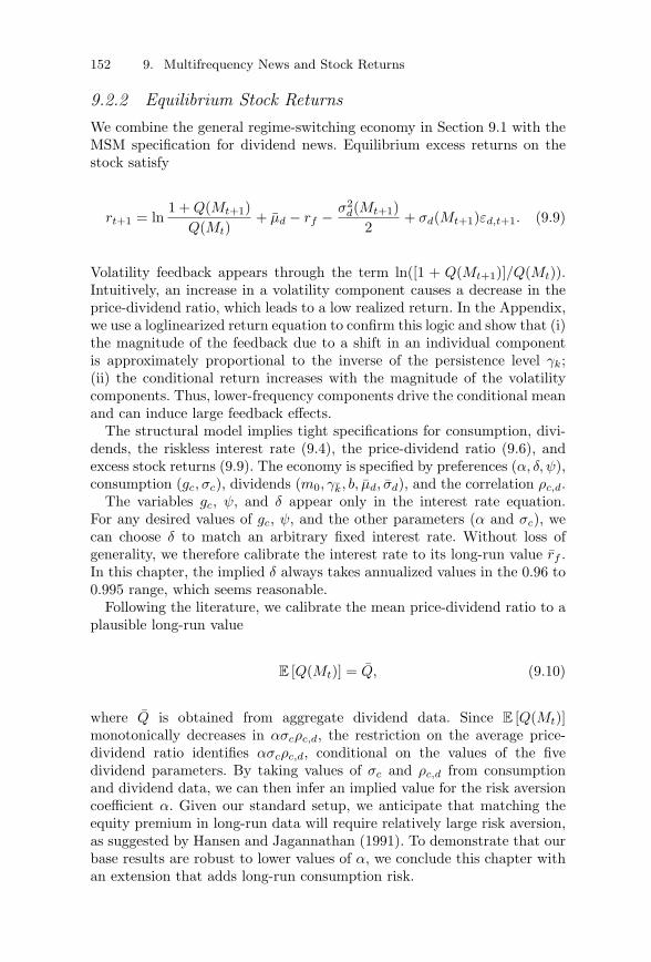
152 9. Multifrequency News and Stock Returns

9.2.2 Equilibrium Stock ReturnsWe combine the general regime-switching economy in Section 9.1 with theMSM specification for dividend news. Equilibrium excess returns on thestock satisfy

rt+1 = ln1 + Q(Mt+1)

Q(Mt)+ μd − rf − σ2

d(Mt+1)2

+ σd(Mt+1)εd,t+1. (9.9)

Volatility feedback appears through the term ln([1 + Q(Mt+1)]/Q(Mt)).Intuitively, an increase in a volatility component causes a decrease in theprice-dividend ratio, which leads to a low realized return. In the Appendix,we use a loglinearized return equation to confirm this logic and show that (i)the magnitude of the feedback due to a shift in an individual componentis approximately proportional to the inverse of the persistence level γk;(ii) the conditional return increases with the magnitude of the volatilitycomponents. Thus, lower-frequency components drive the conditional meanand can induce large feedback effects.

The structural model implies tight specifications for consumption, divi-dends, the riskless interest rate (9.4), the price-dividend ratio (9.6), andexcess stock returns (9.9). The economy is specified by preferences (α, δ, ψ),consumption (gc, σc), dividends (m0, γk, b, μd, σd), and the correlation ρc,d.

The variables gc, ψ, and δ appear only in the interest rate equation.For any desired values of gc, ψ, and the other parameters (α and σc), wecan choose δ to match an arbitrary fixed interest rate. Without loss ofgenerality, we therefore calibrate the interest rate to its long-run value rf .In this chapter, the implied δ always takes annualized values in the 0.96 to0.995 range, which seems reasonable.

Following the literature, we calibrate the mean price-dividend ratio to aplausible long-run value

E [Q(Mt)] = Q, (9.10)

where Q is obtained from aggregate dividend data. Since E [Q(Mt)]monotonically decreases in ασcρc,d, the restriction on the average price-dividend ratio identifies ασcρc,d, conditional on the values of the fivedividend parameters. By taking values of σc and ρc,d from consumptionand dividend data, we can then infer an implied value for the risk aversioncoefficient α. Given our standard setup, we anticipate that matching theequity premium in long-run data will require relatively large risk aversion,as suggested by Hansen and Jagannathan (1991). To demonstrate that ourbase results are robust to lower values of α, we conclude this chapter withan extension that adds long-run consumption risk.

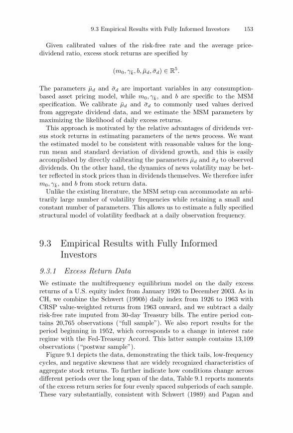
9.3 Empirical Results with Fully Informed Investors 153

Given calibrated values of the risk-free rate and the average price-dividend ratio, excess stock returns are specified by

(m0, γk, b, μd, σd) ∈ R5.

The parameters μd and σd are important variables in any consumption-based asset pricing model, while m0, γk, and b are specific to the MSMspecification. We calibrate μd and σd to commonly used values derivedfrom aggregate dividend data, and we estimate the MSM parameters bymaximizing the likelihood of daily excess returns.

This approach is motivated by the relative advantages of dividends ver-sus stock returns in estimating parameters of the news process. We wantthe estimated model to be consistent with reasonable values for the long-run mean and standard deviation of dividend growth, and this is easilyaccomplished by directly calibrating the parameters μd and σd to observeddividends. On the other hand, the dynamics of news volatility may be bet-ter reflected in stock prices than in dividends themselves. We therefore inferm0, γk, and b from stock return data.

Unlike the existing literature, the MSM setup can accommodate an arbi-trarily large number of volatility frequencies while retaining a small andconstant number of parameters. This allows us to estimate a fully specifiedstructural model of volatility feedback at a daily observation frequency.

9.3 Empirical Results with Fully InformedInvestors

9.3.1 Excess Return DataWe estimate the multifrequency equilibrium model on the daily excessreturns of a U.S. equity index from January 1926 to December 2003. As inCH, we combine the Schwert (1990b) daily index from 1926 to 1963 withCRSP value-weighted returns from 1963 onward, and we subtract a dailyrisk-free rate imputed from 30-day Treasury bills. The entire period con-tains 20,765 observations (“full sample”). We also report results for theperiod beginning in 1952, which corresponds to a change in interest rateregime with the Fed-Treasury Accord. This latter sample contains 13,109observations (“postwar sample”).

Figure 9.1 depicts the data, demonstrating the thick tails, low-frequencycycles, and negative skewness that are widely recognized characteristics ofaggregate stock returns. To further indicate how conditions change acrossdifferent periods over the long span of the data, Table 9.1 reports momentsof the excess return series for four evenly spaced subperiods of each sample.These vary substantially, consistent with Schwert (1989) and Pagan and

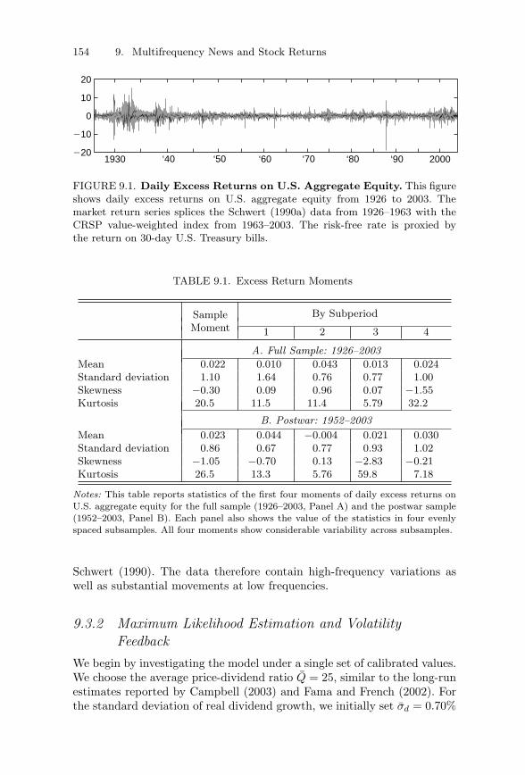
154 9. Multifrequency News and Stock Returns

1930 ‘40 ‘50 ‘60 ‘70 ‘80 ‘90 2000220

210

0

10

20

FIGURE 9.1. Daily Excess Returns on U.S. Aggregate Equity. This figureshows daily excess returns on U.S. aggregate equity from 1926 to 2003. Themarket return series splices the Schwert (1990a) data from 1926–1963 with theCRSP value-weighted index from 1963–2003. The risk-free rate is proxied bythe return on 30-day U.S. Treasury bills.

TABLE 9.1. Excess Return Moments

SampleMoment

By Subperiod

1 2 3 4

A. Full Sample: 1926–2003Mean 0.022 0.010 0.043 0.013 0.024Standard deviation 1.10 1.64 0.76 0.77 1.00Skewness −0.30 0.09 0.96 0.07 −1.55Kurtosis 20.5 11.5 11.4 5.79 32.2

B. Postwar: 1952–2003Mean 0.023 0.044 −0.004 0.021 0.030Standard deviation 0.86 0.67 0.77 0.93 1.02Skewness −1.05 −0.70 0.13 −2.83 −0.21Kurtosis 26.5 13.3 5.76 59.8 7.18

Notes: This table reports statistics of the first four moments of daily excess returns onU.S. aggregate equity for the full sample (1926–2003, Panel A) and the postwar sample(1952–2003, Panel B). Each panel also shows the value of the statistics in four evenlyspaced subsamples. All four moments show considerable variability across subsamples.

Schwert (1990). The data therefore contain high-frequency variations aswell as substantial movements at low frequencies.

9.3.2 Maximum Likelihood Estimation and VolatilityFeedback

We begin by investigating the model under a single set of calibrated values.We choose the average price-dividend ratio Q = 25, similar to the long-runestimates reported by Campbell (2003) and Fama and French (2002). Forthe standard deviation of real dividend growth, we initially set σd = 0.70%

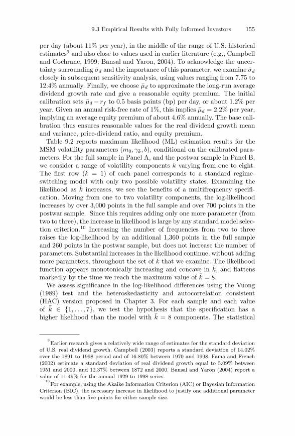
9.3 Empirical Results with Fully Informed Investors 155

per day (about 11% per year), in the middle of the range of U.S. historicalestimates9 and also close to values used in earlier literature (e.g., Campbelland Cochrane, 1999; Bansal and Yaron, 2004). To acknowledge the uncer-tainty surrounding σd and the importance of this parameter, we examine σd

closely in subsequent sensitivity analysis, using values ranging from 7.75 to12.4% annually. Finally, we choose μd to approximate the long-run averagedividend growth rate and give a reasonable equity premium. The initialcalibration sets μd − rf to 0.5 basis points (bp) per day, or about 1.2% peryear. Given an annual risk-free rate of 1%, this implies μd = 2.2% per year,implying an average equity premium of about 4.6% annually. The base cali-bration thus ensures reasonable values for the real dividend growth meanand variance, price-dividend ratio, and equity premium.

Table 9.2 reports maximum likelihood (ML) estimation results for theMSM volatility parameters (m0, γk, b), conditional on the calibrated para-meters. For the full sample in Panel A, and the postwar sample in Panel B,we consider a range of volatility components k varying from one to eight.The first row (k = 1) of each panel corresponds to a standard regime-switching model with only two possible volatility states. Examining thelikelihood as k increases, we see the benefits of a multifrequency specifi-cation. Moving from one to two volatility components, the log-likelihoodincreases by over 3,000 points in the full sample and over 700 points in thepostwar sample. Since this requires adding only one more parameter (fromtwo to three), the increase in likelihood is large by any standard model selec-tion criterion.10 Increasing the number of frequencies from two to threeraises the log-likelihood by an additional 1,360 points in the full sampleand 260 points in the postwar sample, but does not increase the number ofparameters. Substantial increases in the likelihood continue, without addingmore parameters, throughout the set of k that we examine. The likelihoodfunction appears monotonically increasing and concave in k, and flattensmarkedly by the time we reach the maximum value of k = 8.

We assess significance in the log-likelihood differences using the Vuong(1989) test and the heteroskedasticity and autocorrelation consistent(HAC) version proposed in Chapter 3. For each sample and each valueof k ∈ {1, . . . , 7}, we test the hypothesis that the specification has ahigher likelihood than the model with k = 8 components. The statistical

9Earlier research gives a relatively wide range of estimates for the standard deviation

of U.S. real dividend growth. Campbell (2003) reports a standard deviation of 14.02%over the 1891 to 1998 period and of 16.80% between 1970 and 1998. Fama and French(2002) estimate a standard deviation of real dividend growth equal to 5.09% between1951 and 2000, and 12.37% between 1872 and 2000. Bansal and Yaron (2004) report avalue of 11.49% for the annual 1929 to 1998 series.

10For example, using the Akaike Information Criterion (AIC) or Bayesian Information

Criterion (BIC), the necessary increase in likelihood to justify one additional parameterwould be less than five points for either sample size.

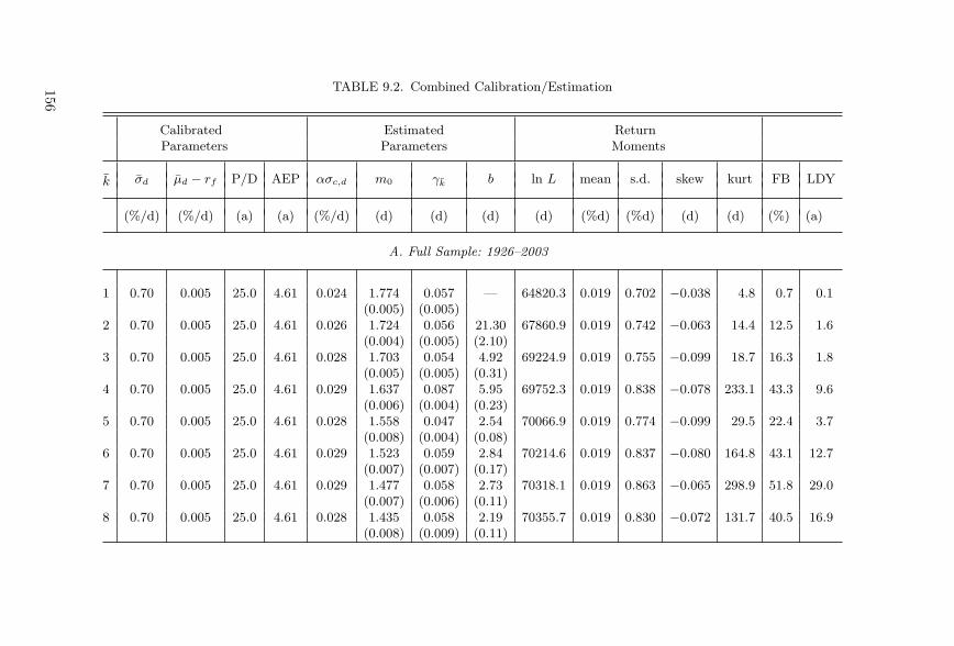
TABLE 9.2. Combined Calibration/Estimation

Calibrated Estimated ReturnParameters Parameters Moments

k σd μd − rf P/D AEP ασc,d m0 γk b ln L mean s.d. skew kurt FB LDY

(%/d) (%/d) (a) (a) (%/d) (d) (d) (d) (d) (%d) (%d) (d) (d) (%) (a)

A. Full Sample: 1926–2003

1 0.70 0.005 25.0 4.61 0.024 1.774 0.057 — 64820.3 0.019 0.702 −0.038 4.8 0.7 0.1(0.005) (0.005)

2 0.70 0.005 25.0 4.61 0.026 1.724 0.056 21.30 67860.9 0.019 0.742 −0.063 14.4 12.5 1.6(0.004) (0.005) (2.10)

3 0.70 0.005 25.0 4.61 0.028 1.703 0.054 4.92 69224.9 0.019 0.755 −0.099 18.7 16.3 1.8(0.005) (0.005) (0.31)

4 0.70 0.005 25.0 4.61 0.029 1.637 0.087 5.95 69752.3 0.019 0.838 −0.078 233.1 43.3 9.6(0.006) (0.004) (0.23)

5 0.70 0.005 25.0 4.61 0.028 1.558 0.047 2.54 70066.9 0.019 0.774 −0.099 29.5 22.4 3.7(0.008) (0.004) (0.08)

6 0.70 0.005 25.0 4.61 0.029 1.523 0.059 2.84 70214.6 0.019 0.837 −0.080 164.8 43.1 12.7(0.007) (0.007) (0.17)

7 0.70 0.005 25.0 4.61 0.029 1.477 0.058 2.73 70318.1 0.019 0.863 −0.065 298.9 51.8 29.0(0.007) (0.006) (0.11)

8 0.70 0.005 25.0 4.61 0.028 1.435 0.058 2.19 70355.7 0.019 0.830 −0.072 131.7 40.5 16.9(0.008) (0.009) (0.11)

156

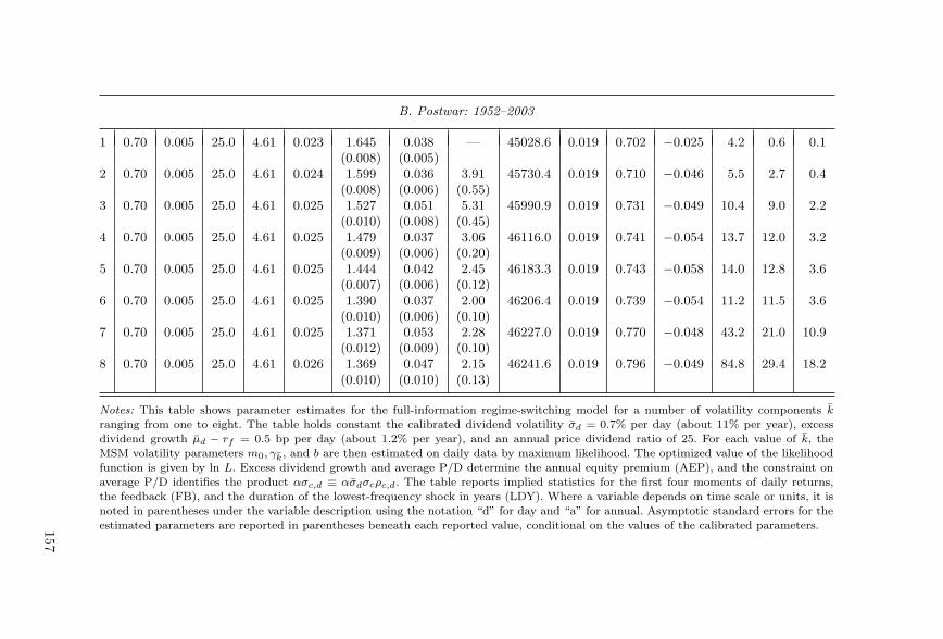
B. Postwar: 1952–2003

1 0.70 0.005 25.0 4.61 0.023 1.645 0.038 — 45028.6 0.019 0.702 −0.025 4.2 0.6 0.1(0.008) (0.005)

2 0.70 0.005 25.0 4.61 0.024 1.599 0.036 3.91 45730.4 0.019 0.710 −0.046 5.5 2.7 0.4(0.008) (0.006) (0.55)

3 0.70 0.005 25.0 4.61 0.025 1.527 0.051 5.31 45990.9 0.019 0.731 −0.049 10.4 9.0 2.2(0.010) (0.008) (0.45)

4 0.70 0.005 25.0 4.61 0.025 1.479 0.037 3.06 46116.0 0.019 0.741 −0.054 13.7 12.0 3.2(0.009) (0.006) (0.20)

5 0.70 0.005 25.0 4.61 0.025 1.444 0.042 2.45 46183.3 0.019 0.743 −0.058 14.0 12.8 3.6(0.007) (0.006) (0.12)

6 0.70 0.005 25.0 4.61 0.025 1.390 0.037 2.00 46206.4 0.019 0.739 −0.054 11.2 11.5 3.6(0.010) (0.006) (0.10)

7 0.70 0.005 25.0 4.61 0.025 1.371 0.053 2.28 46227.0 0.019 0.770 −0.048 43.2 21.0 10.9(0.012) (0.009) (0.10)

8 0.70 0.005 25.0 4.61 0.026 1.369 0.047 2.15 46241.6 0.019 0.796 −0.049 84.8 29.4 18.2(0.010) (0.010) (0.13)

Notes: This table shows parameter estimates for the full-information regime-switching model for a number of volatility components kranging from one to eight. The table holds constant the calibrated dividend volatility σd = 0.7% per day (about 11% per year), excessdividend growth μd − rf = 0.5 bp per day (about 1.2% per year), and an annual price dividend ratio of 25. For each value of k, theMSM volatility parameters m0, γk, and b are then estimated on daily data by maximum likelihood. The optimized value of the likelihoodfunction is given by ln L. Excess dividend growth and average P/D determine the annual equity premium (AEP), and the constraint onaverage P/D identifies the product ασc,d ≡ ασdσcρc,d. The table reports implied statistics for the first four moments of daily returns,the feedback (FB), and the duration of the lowest-frequency shock in years (LDY). Where a variable depends on time scale or units, it isnoted in parentheses under the variable description using the notation “d” for day and “a” for annual. Asymptotic standard errors for theestimated parameters are reported in parentheses beneath each reported value, conditional on the values of the calibrated parameters.157

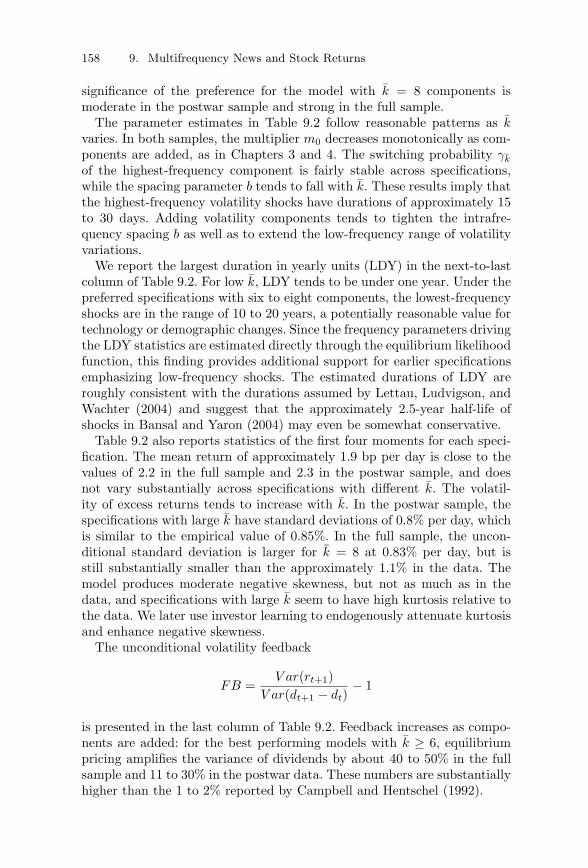
158 9. Multifrequency News and Stock Returns

significance of the preference for the model with k = 8 components ismoderate in the postwar sample and strong in the full sample.

The parameter estimates in Table 9.2 follow reasonable patterns as kvaries. In both samples, the multiplier m0 decreases monotonically as com-ponents are added, as in Chapters 3 and 4. The switching probability γk

of the highest-frequency component is fairly stable across specifications,while the spacing parameter b tends to fall with k. These results imply thatthe highest-frequency volatility shocks have durations of approximately 15to 30 days. Adding volatility components tends to tighten the intrafre-quency spacing b as well as to extend the low-frequency range of volatilityvariations.

We report the largest duration in yearly units (LDY) in the next-to-lastcolumn of Table 9.2. For low k, LDY tends to be under one year. Under thepreferred specifications with six to eight components, the lowest-frequencyshocks are in the range of 10 to 20 years, a potentially reasonable value fortechnology or demographic changes. Since the frequency parameters drivingthe LDY statistics are estimated directly through the equilibrium likelihoodfunction, this finding provides additional support for earlier specificationsemphasizing low-frequency shocks. The estimated durations of LDY areroughly consistent with the durations assumed by Lettau, Ludvigson, andWachter (2004) and suggest that the approximately 2.5-year half-life ofshocks in Bansal and Yaron (2004) may even be somewhat conservative.

Table 9.2 also reports statistics of the first four moments for each speci-fication. The mean return of approximately 1.9 bp per day is close to thevalues of 2.2 in the full sample and 2.3 in the postwar sample, and doesnot vary substantially across specifications with different k. The volatil-ity of excess returns tends to increase with k. In the postwar sample, thespecifications with large k have standard deviations of 0.8% per day, whichis similar to the empirical value of 0.85%. In the full sample, the uncon-ditional standard deviation is larger for k = 8 at 0.83% per day, but isstill substantially smaller than the approximately 1.1% in the data. Themodel produces moderate negative skewness, but not as much as in thedata, and specifications with large k seem to have high kurtosis relative tothe data. We later use investor learning to endogenously attenuate kurtosisand enhance negative skewness.

The unconditional volatility feedback

FB =V ar(rt+1)

V ar(dt+1 − dt)− 1

is presented in the last column of Table 9.2. Feedback increases as compo-nents are added: for the best performing models with k ≥ 6, equilibriumpricing amplifies the variance of dividends by about 40 to 50% in the fullsample and 11 to 30% in the postwar data. These numbers are substantiallyhigher than the 1 to 2% reported by Campbell and Hentschel (1992).

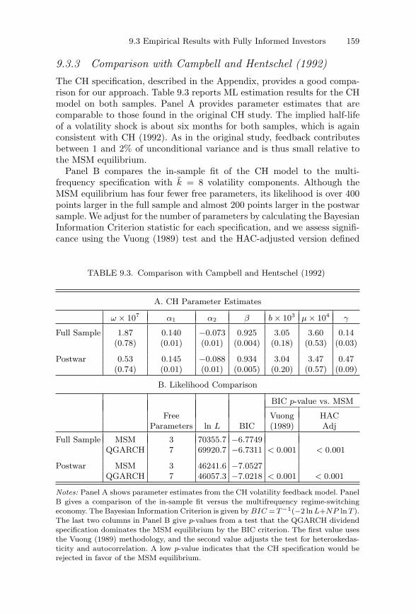
9.3 Empirical Results with Fully Informed Investors 159

9.3.3 Comparison with Campbell and Hentschel (1992)The CH specification, described in the Appendix, provides a good compa-rison for our approach. Table 9.3 reports ML estimation results for the CHmodel on both samples. Panel A provides parameter estimates that arecomparable to those found in the original CH study. The implied half-lifeof a volatility shock is about six months for both samples, which is againconsistent with CH (1992). As in the original study, feedback contributesbetween 1 and 2% of unconditional variance and is thus small relative tothe MSM equilibrium.

Panel B compares the in-sample fit of the CH model to the multi-frequency specification with k = 8 volatility components. Although theMSM equilibrium has four fewer free parameters, its likelihood is over 400points larger in the full sample and almost 200 points larger in the postwarsample. We adjust for the number of parameters by calculating the BayesianInformation Criterion statistic for each specification, and we assess signifi-cance using the Vuong (1989) test and the HAC-adjusted version defined

TABLE 9.3. Comparison with Campbell and Hentschel (1992)

A. CH Parameter Estimates

ω × 107 α1 α2 β b × 103 μ × 104 γ

Full Sample 1.87 0.140 −0.073 0.925 3.05 3.60 0.14(0.78) (0.01) (0.01) (0.004) (0.18) (0.53) (0.03)

Postwar 0.53 0.145 −0.088 0.934 3.04 3.47 0.47(0.74) (0.01) (0.01) (0.005) (0.20) (0.57) (0.09)

B. Likelihood Comparison

BIC p-value vs. MSM

Free Vuong HACParameters ln L BIC (1989) Adj

Full Sample MSM 3 70355.7 −6.7749QGARCH 7 69920.7 −6.7311 < 0.001 < 0.001

Postwar MSM 3 46241.6 −7.0527QGARCH 7 46057.3 −7.0218 < 0.001 < 0.001

Notes: Panel A shows parameter estimates from the CH volatility feedback model. PanelB gives a comparison of the in-sample fit versus the multifrequency regime-switchingeconomy. The Bayesian Information Criterion is given by BIC = T −1(−2 ln L+NP ln T ).The last two columns in Panel B give p-values from a test that the QGARCH dividendspecification dominates the MSM equilibrium by the BIC criterion. The first value usesthe Vuong (1989) methodology, and the second value adjusts the test for heteroskedas-ticity and autocorrelation. A low p-value indicates that the CH specification would berejected in favor of the MSM equilibrium.

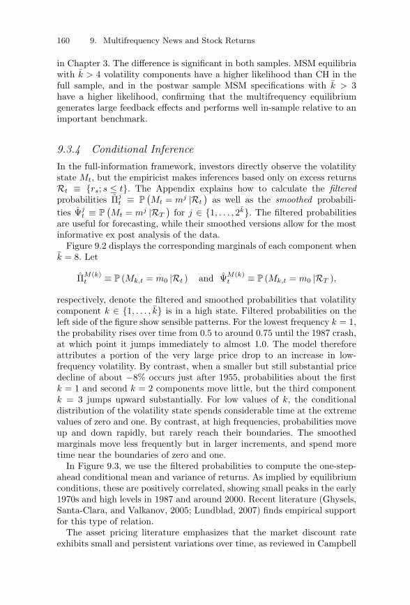
160 9. Multifrequency News and Stock Returns

in Chapter 3. The difference is significant in both samples. MSM equilibriawith k > 4 volatility components have a higher likelihood than CH in thefull sample, and in the postwar sample MSM specifications with k > 3have a higher likelihood, confirming that the multifrequency equilibriumgenerates large feedback effects and performs well in-sample relative to animportant benchmark.

9.3.4 Conditional InferenceIn the full-information framework, investors directly observe the volatilitystate Mt, but the empiricist makes inferences based only on excess returnsRt ≡ {rs; s ≤ t}. The Appendix explains how to calculate the filteredprobabilities Πj

t ≡ P(Mt = mj |Rt

)as well as the smoothed probabili-

ties Ψjt ≡ P

(Mt = mj |RT

)for j ∈ {1, . . . , 2k}. The filtered probabilities

are useful for forecasting, while their smoothed versions allow for the mostinformative ex post analysis of the data.

Figure 9.2 displays the corresponding marginals of each component whenk = 8. Let

ΠM(k)t ≡ P (Mk,t = m0 |Rt ) and ΨM(k)

t ≡ P (Mk,t = m0 |RT ),

respectively, denote the filtered and smoothed probabilities that volatilitycomponent k ∈ {1, . . . , k} is in a high state. Filtered probabilities on theleft side of the figure show sensible patterns. For the lowest frequency k = 1,the probability rises over time from 0.5 to around 0.75 until the 1987 crash,at which point it jumps immediately to almost 1.0. The model thereforeattributes a portion of the very large price drop to an increase in low-frequency volatility. By contrast, when a smaller but still substantial pricedecline of about −8% occurs just after 1955, probabilities about the firstk = 1 and second k = 2 components move little, but the third componentk = 3 jumps upward substantially. For low values of k, the conditionaldistribution of the volatility state spends considerable time at the extremevalues of zero and one. By contrast, at high frequencies, probabilities moveup and down rapidly, but rarely reach their boundaries. The smoothedmarginals move less frequently but in larger increments, and spend moretime near the boundaries of zero and one.

In Figure 9.3, we use the filtered probabilities to compute the one-step-ahead conditional mean and variance of returns. As implied by equilibriumconditions, these are positively correlated, showing small peaks in the early1970s and high levels in 1987 and around 2000. Recent literature (Ghysels,Santa-Clara, and Valkanov, 2005; Lundblad, 2007) finds empirical supportfor this type of relation.

The asset pricing literature emphasizes that the market discount rateexhibits small and persistent variations over time, as reviewed in Campbell

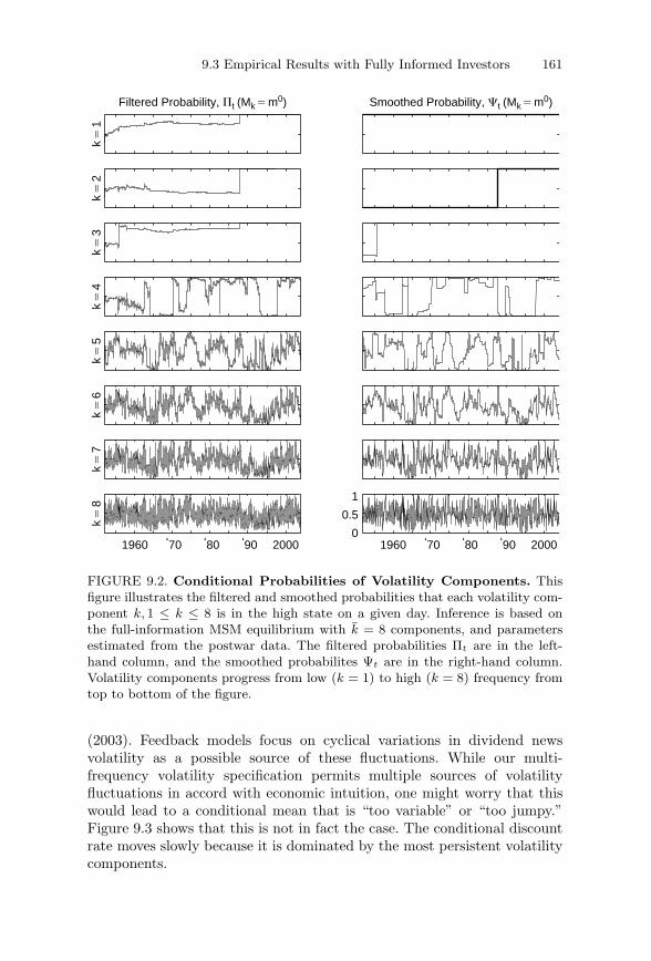
9.3 Empirical Results with Fully Informed Investors 161

k5

1k

52

k5

3k

54

k5

5k

56

k5

7k

58

Filtered Probability, Pt (Mk5 m0) Smoothed Probability, Ct (Mk5 m0)

1960 ‘70 ‘80 ‘90 2000 1960 ‘70 ‘80 ‘90 20000

0.5

1

FIGURE 9.2. Conditional Probabilities of Volatility Components. Thisfigure illustrates the filtered and smoothed probabilities that each volatility com-ponent k, 1 ≤ k ≤ 8 is in the high state on a given day. Inference is based onthe full-information MSM equilibrium with k = 8 components, and parametersestimated from the postwar data. The filtered probabilities Πt are in the left-hand column, and the smoothed probabilites Ψt are in the right-hand column.Volatility components progress from low (k = 1) to high (k = 8) frequency fromtop to bottom of the figure.

(2003). Feedback models focus on cyclical variations in dividend newsvolatility as a possible source of these fluctuations. While our multi-frequency volatility specification permits multiple sources of volatilityfluctuations in accord with economic intuition, one might worry that thiswould lead to a conditional mean that is “too variable” or “too jumpy.”Figure 9.3 shows that this is not in fact the case. The conditional discountrate moves slowly because it is dominated by the most persistent volatilitycomponents.

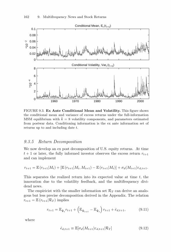
162 9. Multifrequency News and Stock Returns

0

0.02

0.04

0.06

0.08

0.1Conditional Mean, Et (rt +1)

Conditional Volatility, Vart (rt +1)

*102

2

*102

4

1960 1970 1980 1990 20000

2

4

6

8

FIGURE 9.3. Ex Ante Conditional Mean and Volatility. This figure showsthe conditional mean and variance of excess returns under the full-informationMSM equilibrium with k = 8 volatility components, and parameters estimatedfrom postwar data. Conditioning information is the ex ante information set ofreturns up to and including date t.

9.3.5 Return DecompositionWe now develop an ex post decomposition of U.S. equity returns. At timet + 1 or later, the fully informed investor observes the excess return rt+1and can implement

rt+1 = E (rt+1|Mt) + [E (rt+1|Mt, Mt+1) − E (rt+1|Mt)] + σd(Mt+1)εd,t+1.

This separates the realized return into its expected value at time t, theinnovation due to the volatility feedback, and the multifrequency divi-dend news.

The empiricist with the smaller information set RT can derive an analo-gous but less precise decomposition derived in the Appendix. The relationrt+1 = E (rt+1|RT ) implies

rt+1 = EΨtrt+1 +

(EΨt+1

− EΨt

)rt+1 + ed,t+1, (9.11)

where

ed,t+1 ≡ E[σd(Mt+1)εd,t+1|RT ] (9.12)

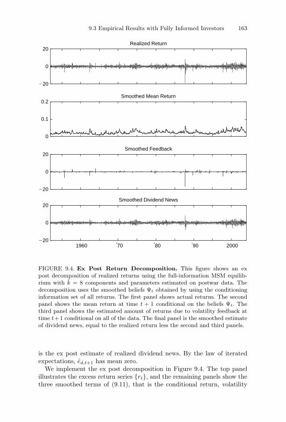
9.3 Empirical Results with Fully Informed Investors 163

0

20

220

Realized Return

0

0.1

0.2Smoothed Mean Return

0

20

220

Smoothed Feedback

1960 ‘70 ‘80 ‘90 2000

0

20

220

Smoothed Dividend News

FIGURE 9.4. Ex Post Return Decomposition. This figure shows an expost decomposition of realized returns using the full-information MSM equilib-rium with k = 8 components and parameters estimated on postwar data. Thedecomposition uses the smoothed beliefs Ψt obtained by using the conditioninginformation set of all returns. The first panel shows actual returns. The secondpanel shows the mean return at time t + 1 conditional on the beliefs Ψt. Thethird panel shows the estimated amount of returns due to volatility feedback attime t+1 conditional on all of the data. The final panel is the smoothed estimateof dividend news, equal to the realized return less the second and third panels.

is the ex post estimate of realized dividend news. By the law of iteratedexpectations, ed,t+1 has mean zero.

We implement the ex post decomposition in Figure 9.4. The top panelillustrates the excess return series {rt}, and the remaining panels show thethree smoothed terms of (9.11), that is the conditional return, volatility

164 9. Multifrequency News and Stock Returns

feedback, and dividend news. The smoothed conditional return in the sec-ond panel of Figure 9.4 shows small persistent variations, very much likethe ex ante conditional return in Figure 9.3. By contrast, the smoothedfeedback in the third panel appears in intermittent bursts. On most days itis small, but its occurrences coincide with the most substantial variationsin the series, and on these days it contributes a large portion of realizedreturns. These features are consistent with the intuition that low-frequencyvolatility changes are infrequent but have a large price impact. This ex postanalysis attributes over half of the 1987 crash to volatility feedback.

In the bottom panel of Figure 9.4, the residual ed,t+1 is the filtered versionof a symmetric MSM process. We calculate its sample moments and findvariance of 0.635, skewness of −0.123, and kurtosis of 8.00. Relative tothe actual return data, the residual variance is approximately 16% smaller,skewness is 88% smaller, and kurtosis is 79% smaller. These findings suggestthat endogenous volatility feedback plays an important role in explainingthe higher moments of returns in our sample.

9.3.6 Alternative CalibrationsWe now examine the robustness of the results to alternative calibrationsof the main economic parameters. Specifically, we explore different val-ues of the calibrated mean μd and standard deviation σd of dividendgrowth and of the average price-dividend ratio Q. For each alterna-tive calibration, we reestimate the volatility parameters (m0, γk, b) of theMSM equilibrium with k = 8 components using the constrained likelihoodfunction.

We also assess how likely each model is to generate return momentssimilar to the data. For each specification, we simulate 1,000 paths of thesame length as the data and calculate the fraction of paths for which a givenstatistic (mean, variance, skewness, kurtosis) exceeds the correspondingempirical moment.

The results of the estimations and simulated p-values are reported inTable 9.4. The first four rows in each panel hold σd constant at 0.7% per day,but allow for varying combinations of Q ∈ {25, 30} and μd−rf ∈ {0.5, 1.0}bp per day, or 1.2% and 2.4% on an annual basis. Increasing the price-dividend ratio Q leads to a lower equity premium (through the Gordongrowth formula), which decreases feedback. To partially compensate, theestimates of m0 and b increase slightly, implying somewhat larger and morepersistent volatility shocks. Overall, the effect of the lower equity premiumdominates, and the feedback measure FB declines as the average price-dividend ratio increases. Similarly, raising the dividend growth rate μd

augments the equity premium and the magnitude of price shocks. Theparameters m0 and b decrease to partially compensate, and the net effect onfeedback is positive. The likelihood tends to increase with μd and decreasewith Q, and thus favors specifications with a larger feedback.

9.4 Learning about Volatility and Endogenous Skewness 165

The final three rows in each panel hold μd and Q constant at their originalvalues and allow dividend volatility σd to increase to 0.8% per day (approx-imately 12.4% annually) or to decrease to 0.6 or 0.5% per day (9.3 and 7.7%annually). These changes in dividend volatility have a considerable impact.When σd is low, the model needs to generate large feedback in order to bet-ter approximate the volatility of excess stock returns. Generally, this tendsto favor larger and more persistent volatility shocks. In the full sample, themodel with σd = 0.5 generates extremely large kurtosis (1,481) and verypersistent shocks (LDY = 160 years); the estimated feedback is over 150%.Larger values of σd generate more moderate feedback in the range of 30 to50%, and have substantially higher likelihood. In the postwar period, forwhich average return volatility is not as high, the model better accommo-dates low values of σd. The highest likelihood in the postwar data occursin the base case in which σd = 0.7.

The simulated p-values show that the model captures well the meanreturn. The empirical skewness is more negative than expected under themodel, but typically within the range of values that can be generated withour sample sizes. In the postwar period, the return volatility is lower thanimplied by the model, but the p-values are not significant. In the full sam-ple, the p-values for the second moment are significant at the 5% level.All of the full-sample specifications and some of the postwar specificationshave significant p-values for a kurtosis that is too large. In summary, largefeedback effects are robust across different calibrations, but kurtosis canbecome excessive when dividend volatility is very low. In the next section,we maintain the symmetric MSM dividend process and show that learn-ing about stochastic volatility can be a powerful method to endogenouslyamplify negative skewness and reduce kurtosis.

9.4 Learning about Volatility and EndogenousSkewness

Financial economists have long considered that investors observe only noisysignals about fundamentals, and a large literature has investigated howBayesian learning about future cash flows and discount rates can affectasset prices and other equilibrium outcomes (e.g., Brennan, 1998; Brennanand Xia, 2001; David, 1997; Guidolin and Timmermann, 2003; Pastor andVeronesi, 2008; Timmermann, 1993, 1996; Veronesi, 1999, 2000, 2004). Fol-lowing this tradition, we assume in this section that investors receive onlyimperfect signals about the volatility state vector Mt. Signal quality con-trols a trade-off between endogenous skewness and kurtosis: as informationquality deteriorates, returns exhibit less kurtosis and more negative skew-ness. We show that (i) the size of the volatility feedback effect is not highlysensitive to the learning environment, and (ii) intermediate informationlevels best capture the higher moments of stock returns.

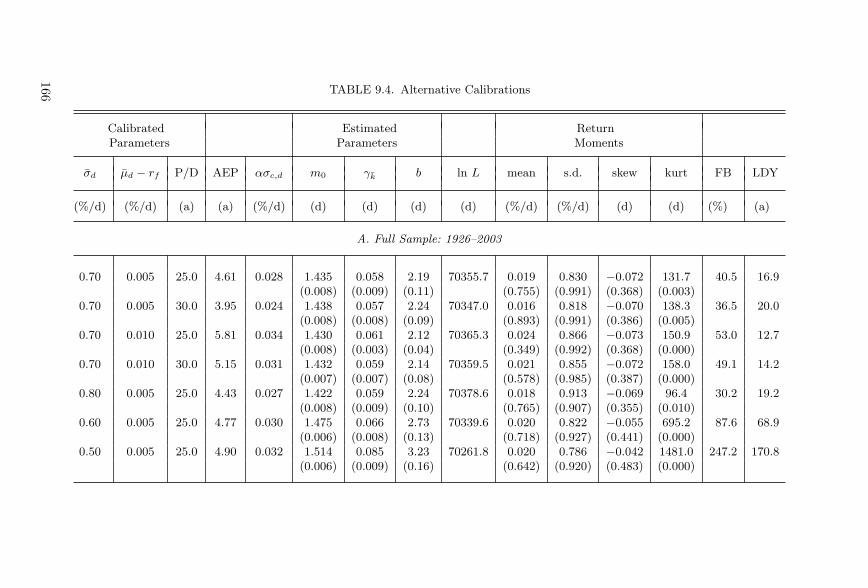
TABLE 9.4. Alternative Calibrations

Calibrated Estimated ReturnParameters Parameters Moments

σd μd − rf P/D AEP ασc,d m0 γk b ln L mean s.d. skew kurt FB LDY

(%/d) (%/d) (a) (a) (%/d) (d) (d) (d) (d) (%/d) (%/d) (d) (d) (%) (a)

A. Full Sample: 1926–2003

0.70 0.005 25.0 4.61 0.028 1.435 0.058 2.19 70355.7 0.019 0.830 −0.072 131.7 40.5 16.9(0.008) (0.009) (0.11) (0.755) (0.991) (0.368) (0.003)

0.70 0.005 30.0 3.95 0.024 1.438 0.057 2.24 70347.0 0.016 0.818 −0.070 138.3 36.5 20.0(0.008) (0.008) (0.09) (0.893) (0.991) (0.386) (0.005)

0.70 0.010 25.0 5.81 0.034 1.430 0.061 2.12 70365.3 0.024 0.866 −0.073 150.9 53.0 12.7(0.008) (0.003) (0.04) (0.349) (0.992) (0.368) (0.000)

0.70 0.010 30.0 5.15 0.031 1.432 0.059 2.14 70359.5 0.021 0.855 −0.072 158.0 49.1 14.2(0.007) (0.007) (0.08) (0.578) (0.985) (0.387) (0.000)

0.80 0.005 25.0 4.43 0.027 1.422 0.059 2.24 70378.6 0.018 0.913 −0.069 96.4 30.2 19.2(0.008) (0.009) (0.10) (0.765) (0.907) (0.355) (0.010)

0.60 0.005 25.0 4.77 0.030 1.475 0.066 2.73 70339.6 0.020 0.822 −0.055 695.2 87.6 68.9(0.006) (0.008) (0.13) (0.718) (0.927) (0.441) (0.000)

0.50 0.005 25.0 4.90 0.032 1.514 0.085 3.23 70261.8 0.020 0.786 −0.042 1481.0 247.2 170.8(0.006) (0.009) (0.16) (0.642) (0.920) (0.483) (0.000)

166

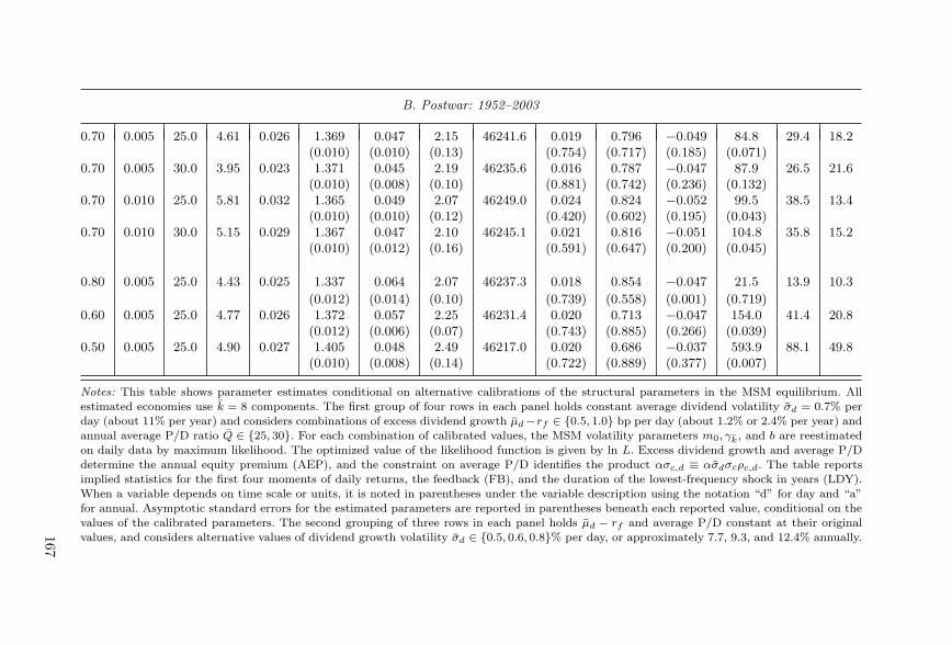
B. Postwar: 1952–2003

0.70 0.005 25.0 4.61 0.026 1.369 0.047 2.15 46241.6 0.019 0.796 −0.049 84.8 29.4 18.2(0.010) (0.010) (0.13) (0.754) (0.717) (0.185) (0.071)

0.70 0.005 30.0 3.95 0.023 1.371 0.045 2.19 46235.6 0.016 0.787 −0.047 87.9 26.5 21.6(0.010) (0.008) (0.10) (0.881) (0.742) (0.236) (0.132)

0.70 0.010 25.0 5.81 0.032 1.365 0.049 2.07 46249.0 0.024 0.824 −0.052 99.5 38.5 13.4(0.010) (0.010) (0.12) (0.420) (0.602) (0.195) (0.043)

0.70 0.010 30.0 5.15 0.029 1.367 0.047 2.10 46245.1 0.021 0.816 −0.051 104.8 35.8 15.2(0.010) (0.012) (0.16) (0.591) (0.647) (0.200) (0.045)

0.80 0.005 25.0 4.43 0.025 1.337 0.064 2.07 46237.3 0.018 0.854 −0.047 21.5 13.9 10.3(0.012) (0.014) (0.10) (0.739) (0.558) (0.001) (0.719)

0.60 0.005 25.0 4.77 0.026 1.372 0.057 2.25 46231.4 0.020 0.713 −0.047 154.0 41.4 20.8(0.012) (0.006) (0.07) (0.743) (0.885) (0.266) (0.039)

0.50 0.005 25.0 4.90 0.027 1.405 0.048 2.49 46217.0 0.020 0.686 −0.037 593.9 88.1 49.8(0.010) (0.008) (0.14) (0.722) (0.889) (0.377) (0.007)

Notes: This table shows parameter estimates conditional on alternative calibrations of the structural parameters in the MSM equilibrium. Allestimated economies use k = 8 components. The first group of four rows in each panel holds constant average dividend volatility σd = 0.7% perday (about 11% per year) and considers combinations of excess dividend growth μd −rf ∈ {0.5, 1.0} bp per day (about 1.2% or 2.4% per year) andannual average P/D ratio Q ∈ {25, 30}. For each combination of calibrated values, the MSM volatility parameters m0, γk, and b are reestimatedon daily data by maximum likelihood. The optimized value of the likelihood function is given by ln L. Excess dividend growth and average P/Ddetermine the annual equity premium (AEP), and the constraint on average P/D identifies the product ασc,d ≡ ασdσcρc,d. The table reportsimplied statistics for the first four moments of daily returns, the feedback (FB), and the duration of the lowest-frequency shock in years (LDY).When a variable depends on time scale or units, it is noted in parentheses under the variable description using the notation “d” for day and “a”for annual. Asymptotic standard errors for the estimated parameters are reported in parentheses beneath each reported value, conditional on thevalues of the calibrated parameters. The second grouping of three rows in each panel holds μd − rf and average P/D constant at their originalvalues, and considers alternative values of dividend growth volatility σd ∈ {0.5, 0.6, 0.8}% per day, or approximately 7.7, 9.3, and 12.4% annually.167

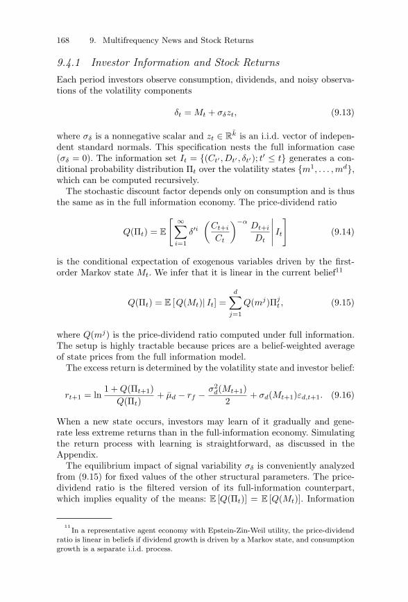
168 9. Multifrequency News and Stock Returns

9.4.1 Investor Information and Stock ReturnsEach period investors observe consumption, dividends, and noisy observa-tions of the volatility components

δt = Mt + σδzt, (9.13)

where σδ is a nonnegative scalar and zt ∈ Rk is an i.i.d. vector of indepen-

dent standard normals. This specification nests the full information case(σδ = 0). The information set It = {(Ct′ , Dt′ , δt′); t′ ≤ t} generates a con-ditional probability distribution Πt over the volatility states {m1, . . . , md},which can be computed recursively.

The stochastic discount factor depends only on consumption and is thusthe same as in the full information economy. The price-dividend ratio

Q(Πt) = E

[ ∞∑

i=1

δ′i(

Ct+i

Ct

)−αDt+i

Dt

∣∣∣∣∣ It

](9.14)

is the conditional expectation of exogenous variables driven by the first-order Markov state Mt. We infer that it is linear in the current belief11

Q(Πt) = E [Q(Mt)| It] =d∑

j=1

Q(mj)Πjt , (9.15)

where Q(mj) is the price-dividend ratio computed under full information.The setup is highly tractable because prices are a belief-weighted averageof state prices from the full information model.

The excess return is determined by the volatility state and investor belief:

rt+1 = ln1 + Q(Πt+1)

Q(Πt)+ μd − rf − σ2

d(Mt+1)2

+ σd(Mt+1)εd,t+1. (9.16)

When a new state occurs, investors may learn of it gradually and gene-rate less extreme returns than in the full-information economy. Simulatingthe return process with learning is straightforward, as discussed in theAppendix.

The equilibrium impact of signal variability σδ is conveniently analyzedfrom (9.15) for fixed values of the other structural parameters. The price-dividend ratio is the filtered version of its full-information counterpart,which implies equality of the means: E [Q(Πt)] = E [Q(Mt)]. Information

11In a representative agent economy with Epstein-Zin-Weil utility, the price-dividend

ratio is linear in beliefs if dividend growth is driven by a Markov state, and consumptiongrowth is a separate i.i.d. process.

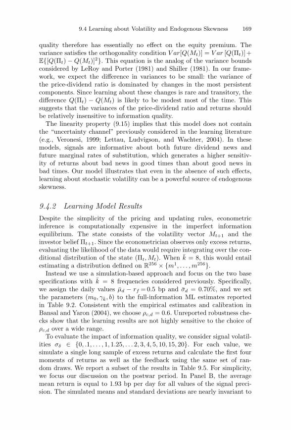
9.4 Learning about Volatility and Endogenous Skewness 169

quality therefore has essentially no effect on the equity premium. Thevariance satisfies the orthogonality condition V ar[Q(Mt)] = V ar [Q(Πt)]+E{[Q(Πt) − Q(Mt)]2}. This equation is the analog of the variance boundsconsidered by LeRoy and Porter (1981) and Shiller (1981). In our frame-work, we expect the difference in variances to be small: the variance ofthe price-dividend ratio is dominated by changes in the most persistentcomponents. Since learning about these changes is rare and transitory, thedifference Q(Πt) − Q(Mt) is likely to be modest most of the time. Thissuggests that the variances of the price-dividend ratio and returns shouldbe relatively insensitive to information quality.

The linearity property (9.15) implies that this model does not containthe “uncertainty channel” previously considered in the learning literature(e.g., Veronesi, 1999; Lettau, Ludvigson, and Wachter, 2004). In thesemodels, signals are informative about both future dividend news andfuture marginal rates of substitution, which generates a higher sensitiv-ity of returns about bad news in good times than about good news inbad times. Our model illustrates that even in the absence of such effects,learning about stochastic volatility can be a powerful source of endogenousskewness.

9.4.2 Learning Model ResultsDespite the simplicity of the pricing and updating rules, econometricinference is computationally expensive in the imperfect informationequilibrium. The state consists of the volatility vector Mt+1 and theinvestor belief Πt+1. Since the econometrician observes only excess returns,evaluating the likelihood of the data would require integrating over the con-ditional distribution of the state (Πt, Mt). When k = 8, this would entailestimating a distribution defined on R

256 × {m1, . . . , m256}.Instead we use a simulation-based approach and focus on the two base

specifications with k = 8 frequencies considered previously. Specifically,we assign the daily values μd − rf = 0.5 bp and σd = 0.70%, and we setthe parameters (m0, γk, b) to the full-information ML estimates reportedin Table 9.2. Consistent with the empirical estimates and calibration inBansal and Yaron (2004), we choose ρc,d = 0.6. Unreported robustness che-cks show that the learning results are not highly sensitive to the choice ofρc,d over a wide range.

To evaluate the impact of information quality, we consider signal volatil-ities σδ ∈ {0, .1, . . . , 1, 1.25, . . . 2, 3, 4, 5, 10, 15, 20}. For each value, wesimulate a single long sample of excess returns and calculate the first fourmoments of returns as well as the feedback using the same set of ran-dom draws. We report a subset of the results in Table 9.5. For simplicity,we focus our discussion on the postwar period. In Panel B, the averagemean return is equal to 1.93 bp per day for all values of the signal preci-sion. The simulated means and standard deviations are nearly invariant to

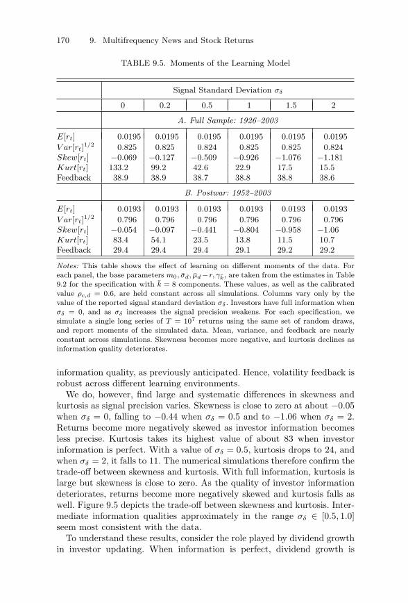
170 9. Multifrequency News and Stock Returns

TABLE 9.5. Moments of the Learning Model

Signal Standard Deviation σδ

0 0.2 0.5 1 1.5 2

A. Full Sample: 1926–2003

E[rt] 0.0195 0.0195 0.0195 0.0195 0.0195 0.0195V ar[rt]1/2 0.825 0.825 0.824 0.825 0.825 0.824Skew[rt] −0.069 −0.127 −0.509 −0.926 −1.076 −1.181Kurt[rt] 133.2 99.2 42.6 22.9 17.5 15.5Feedback 38.9 38.9 38.7 38.8 38.8 38.6

B. Postwar: 1952–2003

E[rt] 0.0193 0.0193 0.0193 0.0193 0.0193 0.0193V ar[rt]1/2 0.796 0.796 0.796 0.796 0.796 0.796Skew[rt] −0.054 −0.097 −0.441 −0.804 −0.958 −1.06Kurt[rt] 83.4 54.1 23.5 13.8 11.5 10.7Feedback 29.4 29.4 29.4 29.1 29.2 29.2

Notes: This table shows the effect of learning on different moments of the data. Foreach panel, the base parameters m0, σd, μd −r, γk, are taken from the estimates in Table9.2 for the specification with k = 8 components. These values, as well as the calibratedvalue ρc,d = 0.6, are held constant across all simulations. Columns vary only by thevalue of the reported signal standard deviation σδ . Investors have full information whenσδ = 0, and as σδ increases the signal precision weakens. For each specification, wesimulate a single long series of T = 107 returns using the same set of random draws,and report moments of the simulated data. Mean, variance, and feedback are nearlyconstant across simulations. Skewness becomes more negative, and kurtosis declines asinformation quality deteriorates.

information quality, as previously anticipated. Hence, volatility feedback isrobust across different learning environments.

We do, however, find large and systematic differences in skewness andkurtosis as signal precision varies. Skewness is close to zero at about −0.05when σδ = 0, falling to −0.44 when σδ = 0.5 and to −1.06 when σδ = 2.Returns become more negatively skewed as investor information becomesless precise. Kurtosis takes its highest value of about 83 when investorinformation is perfect. With a value of σδ = 0.5, kurtosis drops to 24, andwhen σδ = 2, it falls to 11. The numerical simulations therefore confirm thetrade-off between skewness and kurtosis. With full information, kurtosis islarge but skewness is close to zero. As the quality of investor informationdeteriorates, returns become more negatively skewed and kurtosis falls aswell. Figure 9.5 depicts the trade-off between skewness and kurtosis. Inter-mediate information qualities approximately in the range σδ ∈ [0.5, 1.0]seem most consistent with the data.

To understand these results, consider the role played by dividend growthin investor updating. When information is perfect, dividend growth is

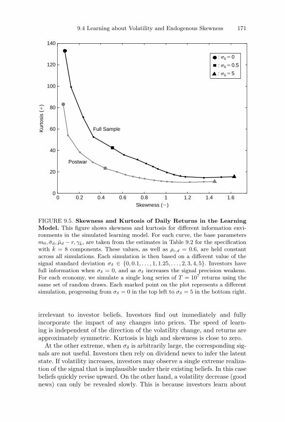
9.4 Learning about Volatility and Endogenous Skewness 171

0 0.2 0.4 0.6 0.8 1 1.2 1.4 1.60

20

40

60

80

100

120

140

Postwar

Full Sample

: sd 5 0

: sd 5 0.5

: sd 5 5

Skewness (2)

Kur

tosi

s (1

)

FIGURE 9.5. Skewness and Kurtosis of Daily Returns in the LearningModel. This figure shows skewness and kurtosis for different information envi-ronments in the simulated learning model. For each curve, the base parametersm0, σd, μd − r, γk, are taken from the estimates in Table 9.2 for the specificationwith k = 8 components. These values, as well as ρc,d = 0.6, are held constantacross all simulations. Each simulation is then based on a different value of thesignal standard deviation σδ ∈ {0, 0.1, . . . , 1, 1.25, . . . , 2, 3, 4, 5}. Investors havefull information when σδ = 0, and as σδ increases the signal precision weakens.For each economy, we simulate a single long series of T = 107 returns using thesame set of random draws. Each marked point on the plot represents a differentsimulation, progressing from σδ = 0 in the top left to σδ = 5 in the bottom right.

irrelevant to investor beliefs. Investors find out immediately and fullyincorporate the impact of any changes into prices. The speed of learn-ing is independent of the direction of the volatility change, and returns areapproximately symmetric. Kurtosis is high and skewness is close to zero.

At the other extreme, when σδ is arbitrarily large, the corresponding sig-nals are not useful. Investors then rely on dividend news to infer the latentstate. If volatility increases, investors may observe a single extreme realiza-tion of the signal that is implausible under their existing beliefs. In this casebeliefs quickly revise upward. On the other hand, a volatility decrease (goodnews) can only be revealed slowly. This is because investors learn about

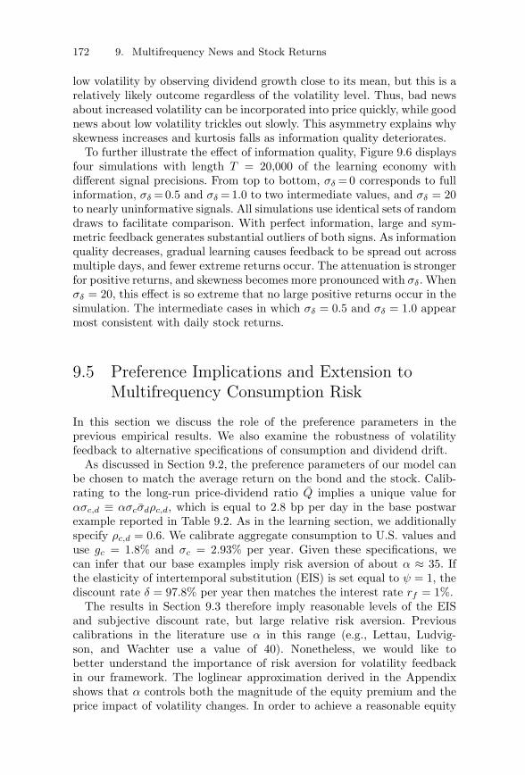
172 9. Multifrequency News and Stock Returns

low volatility by observing dividend growth close to its mean, but this is arelatively likely outcome regardless of the volatility level. Thus, bad newsabout increased volatility can be incorporated into price quickly, while goodnews about low volatility trickles out slowly. This asymmetry explains whyskewness increases and kurtosis falls as information quality deteriorates.

To further illustrate the effect of information quality, Figure 9.6 displaysfour simulations with length T = 20,000 of the learning economy withdifferent signal precisions. From top to bottom, σδ = 0 corresponds to fullinformation, σδ = 0.5 and σδ = 1.0 to two intermediate values, and σδ = 20to nearly uninformative signals. All simulations use identical sets of randomdraws to facilitate comparison. With perfect information, large and sym-metric feedback generates substantial outliers of both signs. As informationquality decreases, gradual learning causes feedback to be spread out acrossmultiple days, and fewer extreme returns occur. The attenuation is strongerfor positive returns, and skewness becomes more pronounced with σδ. Whenσδ = 20, this effect is so extreme that no large positive returns occur in thesimulation. The intermediate cases in which σδ = 0.5 and σδ = 1.0 appearmost consistent with daily stock returns.

9.5 Preference Implications and Extension toMultifrequency Consumption Risk

In this section we discuss the role of the preference parameters in theprevious empirical results. We also examine the robustness of volatilityfeedback to alternative specifications of consumption and dividend drift.

As discussed in Section 9.2, the preference parameters of our model canbe chosen to match the average return on the bond and the stock. Calib-rating to the long-run price-dividend ratio Q implies a unique value forασc,d ≡ ασcσdρc,d, which is equal to 2.8 bp per day in the base postwarexample reported in Table 9.2. As in the learning section, we additionallyspecify ρc,d = 0.6. We calibrate aggregate consumption to U.S. values anduse gc = 1.8% and σc = 2.93% per year. Given these specifications, wecan infer that our base examples imply risk aversion of about α ≈ 35. Ifthe elasticity of intertemporal substitution (EIS) is set equal to ψ = 1, thediscount rate δ = 97.8% per year then matches the interest rate rf = 1%.

The results in Section 9.3 therefore imply reasonable levels of the EISand subjective discount rate, but large relative risk aversion. Previouscalibrations in the literature use α in this range (e.g., Lettau, Ludvig-son, and Wachter use a value of 40). Nonetheless, we would like tobetter understand the importance of risk aversion for volatility feedbackin our framework. The loglinear approximation derived in the Appendixshows that α controls both the magnitude of the equity premium and theprice impact of volatility changes. In order to achieve a reasonable equity

9.5 Preference Implications and Extension to Multifrequency Consumption Risk 173

Full Information (sd5 0)

Intermediate Information (sd5 0.5)

Intermediate Information (sd5 1.0)

0 0.5 1 1.5 23104

0

10

210

220

20

Ret

urns

(%

)

Poor Information (sd5 20)

FIGURE 9.6. Simulations of Daily Excess Returns in the LearningModel. This figure shows learning economy simulations with length T = 20, 000.All simulations are based on the base parameters estimated from the full sam-ple with k = 8 components: m0 = 1.435, σd = 0.70% per day, μ − rf = 0.5 bpper day, γk = 0.058, and b = 2.19. All simulations also use the identical set ofrandom draws for dividends, signal noises, and multipliers. The only value thatchanges across the panels is the signal variability parameter, σδ. The top panelwhere σδ = 0 corresponds to full investor information; the middle two panelsshow intermediate signal precision; and in the final panel information qualityis poor. Noise in the investor signals attenuates extreme feedback realizations,but attenuation is stronger for positive than negative realizations. This gener-ates increasingly negative skewness and reduces kurtosis as information qualitydeteriorates.

174 9. Multifrequency News and Stock Returns

premium using a lower risk aversion, we need an additional source of riskin stock returns.

Small but persistent variations in the drift and volatility of consumptionhave been empirically documented by Bansal and Lundblad (2002), Bansal,Khatchatrian, and Yaron (2005), and Lettau, Ludvigson, and Wachter(2004). Bansal and Yaron (2004) demonstrate that these variations helpto solve the equity premium puzzle. They calibrate a model in which anautoregressive state with a half-life of about 2.5 years drives the drift andvolatility of consumption. Lettau, Ludvigson, and Wachter estimate a four-state regime-switching model in which the good state has a duration of over30 years.

This earlier research motivates the following extension of our asset pricingmodel. Consumption growth exhibits regime shifts in drift and volatility:

ct − ct−1 = gc(M ′t) + σc(M ′

t)εc,t,

where {εc,t} is i.i.d. N (0, 1) and M ′t ∈ R

�+ is a multifrequency state vector

with components. Each component of the state M ′t takes the values mc0 >

1 and 2 − mc0 with equal probability. Drift and volatility are specified by

gc(M ′t) ≡ gc − λc

�∑

k=1

(M ′k,t − 1)

σc(M ′t) ≡ σc(M ′

1,t...M′�,t)

1/2.

Consumption volatility is the product of the components M ′k,t, as in the

dividend news process. We define the drift, on the other hand, as the sumof the state components, which permits a symmetric distribution aroundgc. Similarly, the dividend growth process (9.2) exhibits regime switches indrift

μd(Mt) = μd − λd

k∑

k=1

(Mk,t − 1),

as well as the usual MSM volatility (9.8).The extended specification allows us to capture the variations in macro-

economic risk that have been documented at various frequencies in the lit-erature. When λc > 0, a high M ′

k,t implies both a low drift and a highervolatility, consistent with empirical evidence on business cycles. We assume ≤ k, consistent with the idea of consumption smoothing at short horizons.For instance, consumption may be affected by business cycles, technology,and demographic shocks, but not by shorter-lived shocks that can affectdividend news. For simplicity, we assume that the consumption and volatil-ity components are perfectly correlated; that is, M ′

k,t = mc0 if and only

9.5 Preference Implications and Extension to Multifrequency Consumption Risk 175

if Mk,t = m0 for every k. Asset prices are easily derived as shown in theAppendix.

We calibrate the model using statistics reported by Bansal and Yaron(2004). We set aggregate consumption to gc = 1.80% per year and σc =2.89% per year, and dividends satisfy μd = gc and σd = 0.80% per day.There are = 4 consumption components and k = 5 dividend components.We choose the dividend volatility parameter m0 = 1.50, which is close tothe values estimated in Table 9.2, and set mc0 = 1.40. The drift parameterλc satisfies λc(mc0 − 1) = 0.30% on an annualized basis, implying thatthe state-dependent consumption drift varies between 0.6 and 3% per year.Similarly, the dividend drift switches are specified by λd(m0 − 1) = 0.5%,implying state-dependent drifts varying between −0.7 and 4.3% per year.We set the correlation ρc,d to 0.64, and frequencies are specified by b =2.4 and 1/γ1 = 20 years. The duration of the consumption componentstherefore ranges between 1.44 and 20 years, while the shortest dividendduration is 0.6 years. The coefficient of relative risk aversion is α = 10, andthe other preference parameters are ψ = 1.5 and δ = 0.993.

The dynamics of consumption are consistent with the existing literatureand evidence. The standard deviation of consumption growth is almostidentical to the value used by Bansal and Yaron, and consumption growthautocorrelations are 0.032 at a one-year horizon, 0.015 over five years, and0.009 over ten years. These values would be hard to distinguish from whitenoise and are in fact much lower than the autocorrelations in Bansal andYaron. Similarly, the variance ratios do not exceed 1.21 over a 10-year hori-zon, again lower than the values in Bansal and Yaron. Hence, the consump-tion specification appears to be consistent with earlier empirical evidence.

We first shut down the stochastic volatility of dividends by forcing m0 =1.0 and consequently σd(Mt) = σd. This yields a risk premium of 2.16%,an average price-dividend ratio equal to 46.7, and an average risk-free rateequal to 1.02% per year. The variance of the stock return is 4.2% higherthan the dividend variance; that is, FB = 4.2%.

We then reintroduce stochastic volatility in dividends by specifyingm0 = 1.50. The consumption process, stochastic discount factor, and inter-est rate regimes are unchanged. The equity premium on the stock increasesto 3.29%, and the price-dividend ratio falls to 31.1. The price-dividendregimes vary between 22.9 and 37.7. The feedback increases to 25.9%,which is more than six times larger than when dividend volatility is con-stant. The marginal contribution of multifrequency dividend volatility toreturn volatility is thus 25.9%− 4.2% = 21.7%, which is comparable to thefeedback estimates obtained with i.i.d. consumption and high risk aversion.

In sum, by incorporating long-run risks in consumption, we can use alower risk aversion (α = 10) to match the equity premium and still generatea substantial contribution of dividend volatility feedback. The exten-sion also offers a pure regime-switching formulation of long-run risks ina multifrequency environment, opening new directions for future research.

176 9. Multifrequency News and Stock Returns

9.6 Discussion

In this chapter, we develop a tractable asset pricing framework withmultifrequency shocks to fundamentals and discount rates, focusing on adividend news specification with constant mean, multifrequency stochas-tic volatility, and conditionally Gaussian noise. The structural equilibriumwith three free parameters accounts for endogenous skewness, thick tails,time-varying volatility, and sizeable feedback in over 80 years of daily stockreturns.

Two economic mechanisms play important roles. First, endogenousvolatility feedback amplifies dividend variance by 20 to 40% in favoredspecifications, or 10 to 40 times the feedback obtained in the previousliterature (e.g., Campbell and Hentschel, 1992). Feedback from persistentcomponents helps to capture extreme returns, while higher-frequency vari-ations match day-to-day volatility movements. Second, investor learninggenerates substantial endogenous skewness. Building on Veronesi (2000), weconsider investor signals about the volatility state and show that informa-tion quality creates a trade-off between skewness and kurtosis. Intermediateinformation environments best match the data.

The chapter illustrates that a multifrequency approach helps connect thelow-frequency macro-finance and learning literatures with higher-frequencyfinancial econometrics. Convergence of these areas follows from bringingmultifrequency shocks into pure regime-switching economies, which tradi-tionally offer three major benefits: (i) asset pricing is straightforward ina Markov chain setup; (ii) the econometrics of regime-switching, based onsimple filtering theory, is well understood; and (iii) learning is easily incor-porated by using similar filtering techniques. The multifrequency approachexpands the practical range of equilibrium regime-switching economies froma few states to several hundred and from lower frequencies to daily returns.

We develop an extension based on joint modeling of multifrequencyregime switches in consumption and dividends. This generates large feed-back and a reasonable equity premium with moderate values of relativerisk aversion. This framework offers potential for further development,particularly in modeling the impact of long-run risks on high-frequencyfinancial data.

10Multifrequency Jump-Diffusions

The multifractal diffusions considered in Part II are exogenously specifiedand have continuous sample paths. We now endogenize the price pro-cess by considering a continuous-time version of the exchange economydeveloped in Chapter 9. Dividends and consumption follow continuous dif-fusions, but their drift rates and volatilities can undergo discrete Markovswitches. These regime changes in fundamentals trigger endogenous jumpsin asset prices, consistent with the well-known property that discretearrivals of information about cash flows and discount rates can cause pricediscontinuities in equilibrium.

When dividends follow a continuous-time MSM, the construction gen-erates a new class of stochastic processes, which we call multifrequencyjump-diffusions. The stock price displays endogenous jumps of heteroge-neous frequencies, and the largest discontinuities are triggered by the mostpersistent volatility shocks. The model thus produces many small jumpsand fewer large jumps, as in Madan, Carr, and Chang (1998), Carr, Geman,Madan, and Yor (2002), and others. Our equilibrium model contributes tothe literature on jump and Levy processes by endogenizing the heterogeneityof jump sizes, and the association between jump-size and frequency.

We investigate the limiting behavior of the economy when the number ofvolatility components goes to infinity. As in Chapter 7, the dividend processweakly converges to a multifractal diffusion with continuous sample paths.We also show that the equilibrium price-dividend ratio converges to an infi-nite intensity pure jump process with heterogeneous frequencies. Prices arethen the sum of a continuous multifractal diffusion and an infinite intensity,pure jump process, yielding a new stochastic process that we accordinglycall a multifractal jump-diffusion. A jump in the stock price occurs in theneighborhoodofany instant,but theprocess is continuousalmost everywhere.

For simplicity, the chapter focuses mainly on time-separable preferences.The stochastic discount factor is then continuous, and endogenous jumpsin stock valuations are “unpriced” in the sense that they do not affectexpected excess stock returns (e.g., Merton, 1976). In the final section,we obtain priced jumps and endogenous discontinuities in the stochasticdiscount factor by assuming nonseparable preferences, as in Epstein andZin (1989), Weil (1989), and Duffie and Epstein (1992). This extensionprovides additional flexibility in structural modeling of jump-diffusions.

This chapter is based on an earlier paper: “Multifrequency Jump-Diffusions: An Equili-brium Approach” (with A. Fisher), Journal of Mathematical Economics, 44: 207–261,January 2008.

178 10. Multifrequency Jump-Diffusions

10.1 An Equilibrium Model with EndogenousPrice Jumps

This section develops a continuous-time equilibrium model with regime-shifts in the drift and volatility of fundamentals. We do not require thatthe state follows an MSM process, and the setup developed in this sectioncan therefore be used directly in other contexts.

10.1.1 Preferences, Information, and IncomeWe consider an exchange economy with a single consumption good definedon the set of instants t ∈ [0,∞). The information structure is representedby a filtration {Ft} on the probability space (Ω,F , P).

The economy is specified by two independent stochastic processes:a bivariate Brownian motion Zt = (ZY (t), ZD(t)) ∈ R

2 and a random statevector Mt ∈ R

k+, where k is a finite integer. The processes Z and M are

mutually independent and adapted to the filtration {Ft}. The bivariateBrownian Z has zero mean and covariance matrix

(1 ρY,D

ρY,D 1

),

where the correlation coefficient ρY,D = Cov(dZY , dZD)/dt is strictly pos-itive. The vector Mt is a stationary Markov process with right-continuoussample paths.

The economy is populated by a finite set of identical investorsh ∈ {1, . . . , H}, who have homogeneous information, preferences, andendowments. Investors observe the realization of the processes Z and M ,and have information set It = {(Zs, Ms); s ≤ t}. The common utility isgiven by

Ut = E

[∫ +∞

0e−δsu(ct+s)ds

∣∣∣∣ It

],

where the discount rate is a positive constant: δ ∈ (0,∞). The Bernoulliutility u(·) is twice continuously differentiable and satisfies the usualmonotonicity and concavity conditions: u′ > 0 and u′′ < 0. Furthermore,the Inada conditions hold: limc→0 u′(c) = +∞ and limc→+∞ u′(c) = 0.

Every agent continuously receives the exogenous endowment stream Yt ∈(0,∞). The process Yt is identical across the population and follows ageometric Brownian motion with stochastic drift and volatility. Specifically,let gY (·) and σY (·) denote deterministic measurable functions defined onR

k+ and taking values on the real line.

10.1 An Equilibrium Model with Endogenous Price Jumps 179

Condition 7 (Income) The moments E

[∫ t

0 |gY (Ms)| ds]

and E

[∫ t

0 σ2Y

(Ms)ds] are finite, and the exogenous income stream is given by

ln(Yt) ≡ ln(Y0) +∫ t

0

[gY (Ms) − σ2

Y (Ms)2

]ds +

∫ t

0σY (Ms)dZY (s)

at every instant t ∈ [0,∞).

The moment conditions guarantee that the stochastic integrals are welldefined. By Ito’s lemma, the income flow satisfies the stochastic differentialequation

dYt

Yt= gY (Mt)dt + σY (Mt)dZY (t). (10.1)

10.1.2 Financial Markets and EquilibriumAgents can trade two financial assets: a bond and a stock. The bond hasan instantaneous rate of return rf (t), which is endogenously determined inequilibrium. Its net supply is equal to zero.

The stock is a claim on the stochastic dividend stream {Dt}t≥0.

Condition 8 (Dividend process) The dividend stream is given by:

ln(Dt) ≡ ln(D0) +∫ t

0

[gD(Ms) − σ2

D(Ms)2

]ds +

∫ t

0σD(Ms)dZD(s),

where gD(·) and σD(·) are measurable functions defined on Rk+ and valued

in R such that E

[∫ t

0 |gD(Ms)| ds]

< ∞ and E

[∫ t

0 σ2D(Ms)ds

]< ∞ for

all t.

We infer from Ito’s lemma:

dDt

Dt= gD(Mt)dt + σD(Mt)dZD(t). (10.2)

The dividend process Dt has continuous sample paths, but its drift andvolatility can exhibit discontinuities. Every agent is initially endowed withNs ∈ R+ units of stock, where one unit represents one claim on the flowDt. We treat the difference Yt −NsDt as the nontradable component of theendowment flow.1

1Distinguishing between aggregate endowment flow and dividends on public equity iscommon in asset pricing settings. For example, Brennan and Xia (2001) invoke nontradedlabor income as a wedge between the aggregate endowment flow and dividends. In our

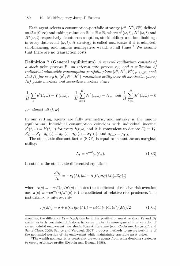
180 10. Multifrequency Jump-Diffusions

Each agent selects a consumption-portfolio strategy (ch, Nh, Bh) definedon Ω× [0,∞) and taking values on R+×R×R, where ch(ω, t), Nh(ω, t) andBh(ω, t) respectively denote consumption, stockholdings and bondholdingsin every date-event (ω, t). A strategy is called admissible if it is adapted,self-financing, and implies nonnegative wealth at all times.2 We assumethat there are no transaction costs.

Definition 7 (General equilibrium) A general equilibrium consists ofa stock price process P , an interest rate process rf , and a collection ofindividual admissible consumption-portfolio plans (ch, Nh, Bh)1≤h≤H , suchthat (i) for every h, (ch, Nh, Bh) maximizes utility over all admissible plans;(ii) goods markets and securities markets clear:

1H

∑

h

ch(t, ω) = Y (t, ω),1H

H∑

h=1

Nh(t, ω) = Ns, and1H

H∑

h=1

Bh(t, ω) = 0

for almost all (t, ω).

In our setting, agents are fully symmetric, and autarky is the uniqueequilibrium. Individual consumption coincides with individual income:ch(t, ω) = Y (t, ω) for every h,t, ω, and it is convenient to denote Ct ≡ Yt,ZC ≡ ZY , gC (.) ≡ gY (.) , σC (.) ≡ σY (.), and ρC,D ≡ ρY,D.

The stochastic discount factor (SDF) is equal to instantaneous marginalutility:

Λt = e−δtu′(Ct). (10.3)

It satisfies the stochastic differential equation:

dΛt

Λt= −rf (Mt)dt − α(Ct)σC(Mt)dZC(t),

where α(c) ≡ −cu′′(c)/u′(c) denotes the coefficient of relative risk aversionand π(c) ≡ −cu′′′(c)/u′′(c) is the coefficient of relative risk prudence. Theinstantaneous interest rate

rf (Mt) = δ + α(Ct)gC(Mt) − α(Ct)π(Ct)σ2C(Mt)/2 (10.4)

economy, the difference Yt − NsDt can be either positive or negative since Yt and Dt

are imperfectly correlated diffusions: hence we prefer the more general interpretation ofan unmodeled endowment flow shock. Recent literature (e.g., Cochrane, Longstaff, andSanta-Clara, 2008; Santos and Veronesi, 2005) proposes methods to ensure positivity ofthe nontraded portion of the endowment while maintaining tractable asset prices.

2The wealth nonnegativity constraint prevents agents from using doubling strategiesto create arbitrage profits (Dybvig and Huang, 1988).

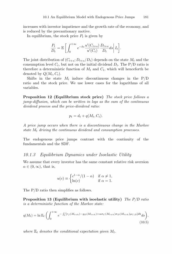
10.1 An Equilibrium Model with Endogenous Price Jumps 181

increases with investor impatience and the growth rate of the economy, andis reduced by the precautionary motive.

In equilibrium, the stock price Pt is given by

Pt

Dt= E

[∫ +∞

0e−δs u′(Ct+s)

u′(Ct)Dt+s

Dtds

∣∣∣∣ It

].

The joint distribution of (Ct+s;Dt+s/Dt) depends on the state Mt and theconsumption level Ct, but not on the initial dividend Dt. The P/D ratio istherefore a deterministic function of Mt and Ct, which will henceforth bedenoted by Q(Mt, Ct).

Shifts in the state Mt induce discontinuous changes in the P/Dratio and the stock price. We use lower cases for the logarithms of allvariables.

Proposition 12 (Equilibrium stock price) The stock price follows ajump-diffusion, which can be written in logs as the sum of the continuousdividend process and the price-dividend ratio:

pt = dt + q(Mt, Ct).

A price jump occurs when there is a discontinuous change in the Markovstate Mt driving the continuous dividend and consumption processes.

The endogenous price jumps contrast with the continuity of thefundamentals and the SDF.

10.1.3 Equilibrium Dynamics under Isoelastic UtilityWe assume that every investor has the same constant relative risk aversionα ∈ (0,∞), that is,

u(c) ≡{

c1−α/(1 − α) if α �= 1,ln(c) if α = 1.

The P/D ratio then simplifies as follows.

Proposition 13 (Equilibrium with isoelastic utility) The P/D ratiois a deterministic function of the Markov state:

q(Mt) = ln Et

(∫ +∞

0e−

∫ s0 [rf (Mt+h)−gD(Mt+h)+ασC(Mt+h)σD(Mt+h)ρC,D]dhds

)

,

(10.5)

where Et denotes the conditional expectation given Mt.

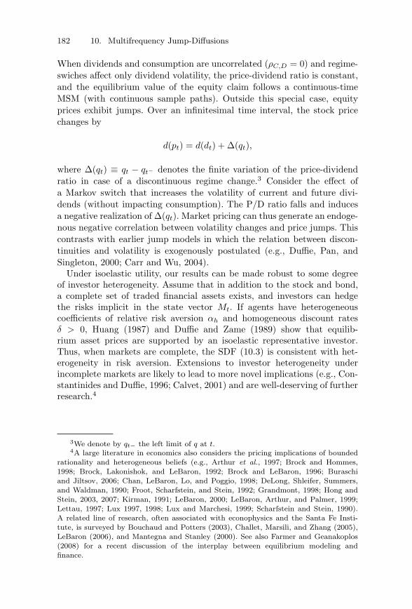
182 10. Multifrequency Jump-Diffusions

When dividends and consumption are uncorrelated (ρC,D = 0) and regime-swiches affect only dividend volatility, the price-dividend ratio is constant,and the equilibrium value of the equity claim follows a continuous-timeMSM (with continuous sample paths). Outside this special case, equityprices exhibit jumps. Over an infinitesimal time interval, the stock pricechanges by

d(pt) = d(dt) + Δ(qt),

where Δ(qt) ≡ qt − qt− denotes the finite variation of the price-dividendratio in case of a discontinuous regime change.3 Consider the effect ofa Markov switch that increases the volatility of current and future divi-dends (without impacting consumption). The P/D ratio falls and inducesa negative realization of Δ(qt). Market pricing can thus generate an endoge-nous negative correlation between volatility changes and price jumps. Thiscontrasts with earlier jump models in which the relation between discon-tinuities and volatility is exogenously postulated (e.g., Duffie, Pan, andSingleton, 2000; Carr and Wu, 2004).

Under isoelastic utility, our results can be made robust to some degreeof investor heterogeneity. Assume that in addition to the stock and bond,a complete set of traded financial assets exists, and investors can hedgethe risks implicit in the state vector Mt. If agents have heterogeneouscoefficients of relative risk aversion αh and homogeneous discount ratesδ > 0, Huang (1987) and Duffie and Zame (1989) show that equilib-rium asset prices are supported by an isoelastic representative investor.Thus, when markets are complete, the SDF (10.3) is consistent with het-erogeneity in risk aversion. Extensions to investor heterogeneity underincomplete markets are likely to lead to more novel implications (e.g., Con-stantinides and Duffie, 1996; Calvet, 2001) and are well-deserving of furtherresearch.4

3We denote by qt− the left limit of q at t.4A large literature in economics also considers the pricing implications of bounded

rationality and heterogeneous beliefs (e.g., Arthur et al., 1997; Brock and Hommes,1998; Brock, Lakonishok, and LeBaron, 1992; Brock and LeBaron, 1996; Buraschiand Jiltsov, 2006; Chan, LeBaron, Lo, and Poggio, 1998; DeLong, Shleifer, Summers,and Waldman, 1990; Froot, Scharfstein, and Stein, 1992; Grandmont, 1998; Hong andStein, 2003, 2007; Kirman, 1991; LeBaron, 2000; LeBaron, Arthur, and Palmer, 1999;Lettau, 1997; Lux 1997, 1998; Lux and Marchesi, 1999; Scharfstein and Stein, 1990).A related line of research, often associated with econophysics and the Santa Fe Insti-tute, is surveyed by Bouchaud and Potters (2003), Challet, Marsili, and Zhang (2005),LeBaron (2006), and Mantegna and Stanley (2000). See also Farmer and Geanakoplos(2008) for a recent discussion of the interplay between equilibrium modeling andfinance.

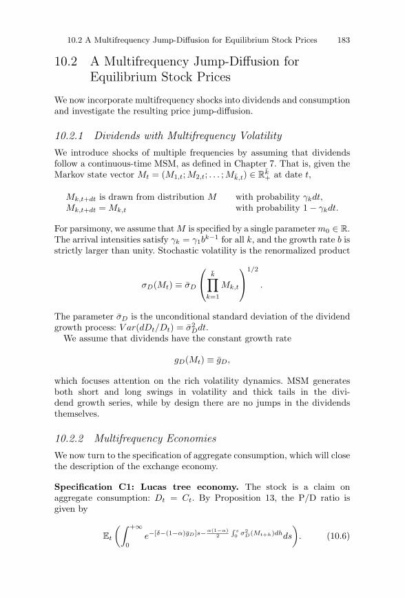
10.2 A Multifrequency Jump-Diffusion for Equilibrium Stock Prices 183

10.2 A Multifrequency Jump-Diffusion forEquilibrium Stock Prices

We now incorporate multifrequency shocks into dividends and consumptionand investigate the resulting price jump-diffusion.

10.2.1 Dividends with Multifrequency VolatilityWe introduce shocks of multiple frequencies by assuming that dividendsfollow a continuous-time MSM, as defined in Chapter 7. That is, given theMarkov state vector Mt = (M1,t;M2,t; . . . ;Mk,t) ∈ R

k+ at date t,

Mk,t+dt is drawn from distribution M with probability γkdt,Mk,t+dt = Mk,t with probability 1 − γkdt.

For parsimony, we assume that M is specified by a single parameter m0 ∈ R.The arrival intensities satisfy γk = γ1b

k−1 for all k, and the growth rate b isstrictly larger than unity. Stochastic volatility is the renormalized product

σD(Mt) ≡ σD

⎛

⎝k∏

k=1

Mk,t

⎞

⎠1/2

.

The parameter σD is the unconditional standard deviation of the dividendgrowth process: V ar(dDt/Dt) = σ2

Ddt.We assume that dividends have the constant growth rate

gD(Mt) ≡ gD,

which focuses attention on the rich volatility dynamics. MSM generatesboth short and long swings in volatility and thick tails in the divi-dend growth series, while by design there are no jumps in the dividendsthemselves.

10.2.2 Multifrequency EconomiesWe now turn to the specification of aggregate consumption, which will closethe description of the exchange economy.

Specification C1: Lucas tree economy. The stock is a claim onaggregate consumption: Dt = Ct. By Proposition 13, the P/D ratio isgiven by

Et

(∫ +∞

0e−[δ−(1−α)gD]s− α(1−α)

2

∫ s0 σ2

D(Mt+h)dhds

). (10.6)

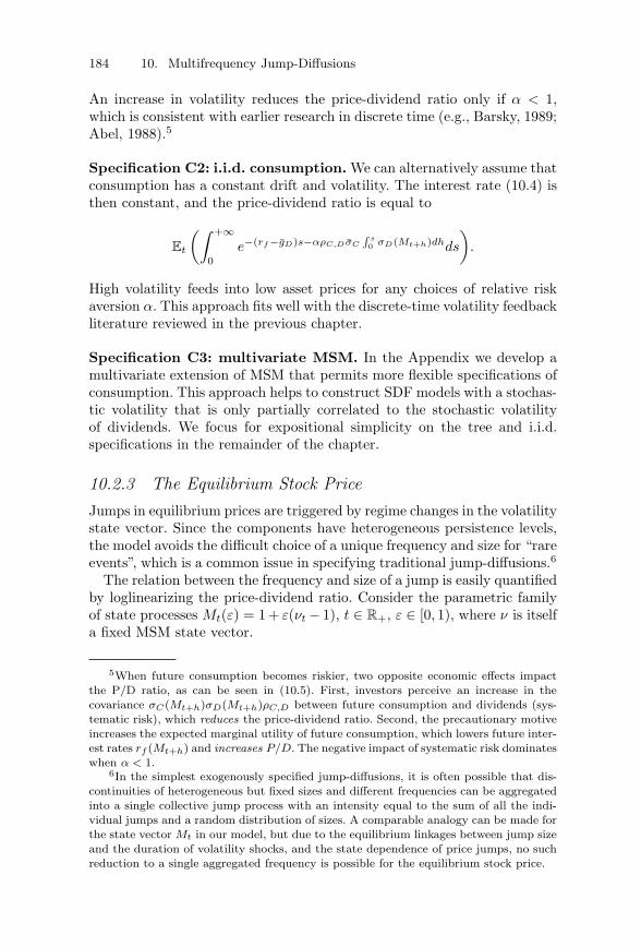
184 10. Multifrequency Jump-Diffusions

An increase in volatility reduces the price-dividend ratio only if α < 1,which is consistent with earlier research in discrete time (e.g., Barsky, 1989;Abel, 1988).5

Specification C2: i.i.d. consumption. We can alternatively assume thatconsumption has a constant drift and volatility. The interest rate (10.4) isthen constant, and the price-dividend ratio is equal to

Et

(∫ +∞

0e−(rf −gD)s−αρC,DσC

∫ s0 σD(Mt+h)dhds

).

High volatility feeds into low asset prices for any choices of relative riskaversion α. This approach fits well with the discrete-time volatility feedbackliterature reviewed in the previous chapter.

Specification C3: multivariate MSM. In the Appendix we develop amultivariate extension of MSM that permits more flexible specifications ofconsumption. This approach helps to construct SDF models with a stochas-tic volatility that is only partially correlated to the stochastic volatilityof dividends. We focus for expositional simplicity on the tree and i.i.d.specifications in the remainder of the chapter.

10.2.3 The Equilibrium Stock PriceJumps in equilibrium prices are triggered by regime changes in the volatilitystate vector. Since the components have heterogeneous persistence levels,the model avoids the difficult choice of a unique frequency and size for “rareevents”, which is a common issue in specifying traditional jump-diffusions.6

The relation between the frequency and size of a jump is easily quantifiedby loglinearizing the price-dividend ratio. Consider the parametric familyof state processes Mt(ε) = 1 + ε(νt − 1), t ∈ R+, ε ∈ [0, 1), where ν is itselfa fixed MSM state vector.

5When future consumption becomes riskier, two opposite economic effects impactthe P/D ratio, as can be seen in (10.5). First, investors perceive an increase in thecovariance σC(Mt+h)σD(Mt+h)ρC,D between future consumption and dividends (sys-tematic risk), which reduces the price-dividend ratio. Second, the precautionary motiveincreases the expected marginal utility of future consumption, which lowers future inter-est rates rf (Mt+h) and increases P/D. The negative impact of systematic risk dominateswhen α < 1.

6In the simplest exogenously specified jump-diffusions, it is often possible that dis-continuities of heterogeneous but fixed sizes and different frequencies can be aggregatedinto a single collective jump process with an intensity equal to the sum of all the indi-vidual jumps and a random distribution of sizes. A comparable analogy can be made forthe state vector Mt in our model, but due to the equilibrium linkages between jump sizeand the duration of volatility shocks, and the state dependence of price jumps, no suchreduction to a single aggregated frequency is possible for the equilibrium stock price.

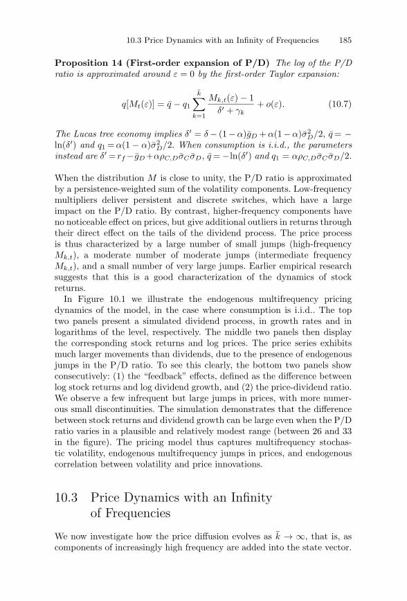
10.3 Price Dynamics with an Infinity of Frequencies 185

Proposition 14 (First-order expansion of P/D) The log of the P/Dratio is approximated around ε = 0 by the first-order Taylor expansion:

q[Mt(ε)] = q − q1

k∑

k=1

Mk,t(ε) − 1δ′ + γk

+ o(ε). (10.7)

The Lucas tree economy implies δ′ = δ − (1 − α)gD + α(1 − α)σ2D/2, q = −

ln(δ′) and q1 =α(1 − α)σ2D/2. When consumption is i.i.d., the parameters

instead are δ′ = rf −gD+αρC,DσC σD, q = −ln(δ′) and q1 = αρC,DσC σD/2.

When the distribution M is close to unity, the P/D ratio is approximatedby a persistence-weighted sum of the volatility components. Low-frequencymultipliers deliver persistent and discrete switches, which have a largeimpact on the P/D ratio. By contrast, higher-frequency components haveno noticeable effect on prices, but give additional outliers in returns throughtheir direct effect on the tails of the dividend process. The price processis thus characterized by a large number of small jumps (high-frequencyMk,t), a moderate number of moderate jumps (intermediate frequencyMk,t), and a small number of very large jumps. Earlier empirical researchsuggests that this is a good characterization of the dynamics of stockreturns.

In Figure 10.1 we illustrate the endogenous multifrequency pricingdynamics of the model, in the case where consumption is i.i.d.. The toptwo panels present a simulated dividend process, in growth rates and inlogarithms of the level, respectively. The middle two panels then displaythe corresponding stock returns and log prices. The price series exhibitsmuch larger movements than dividends, due to the presence of endogenousjumps in the P/D ratio. To see this clearly, the bottom two panels showconsecutively: (1) the “feedback” effects, defined as the difference betweenlog stock returns and log dividend growth, and (2) the price-dividend ratio.We observe a few infrequent but large jumps in prices, with more numer-ous small discontinuities. The simulation demonstrates that the differencebetween stock returns and dividend growth can be large even when the P/Dratio varies in a plausible and relatively modest range (between 26 and 33in the figure). The pricing model thus captures multifrequency stochas-tic volatility, endogenous multifrequency jumps in prices, and endogenouscorrelation between volatility and price innovations.

10.3 Price Dynamics with an Infinityof Frequencies

We now investigate how the price diffusion evolves as k → ∞, that is, ascomponents of increasingly high frequency are added into the state vector.

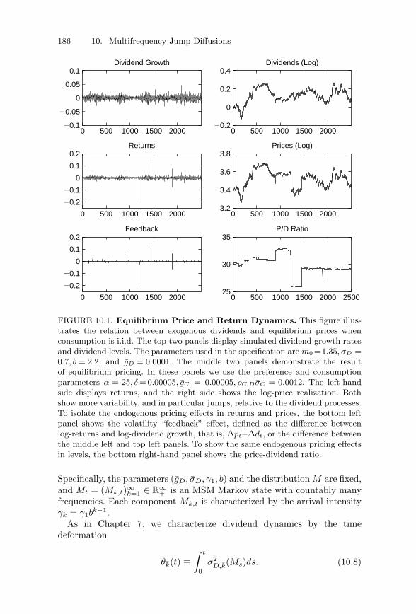
186 10. Multifrequency Jump-Diffusions

0 500 1000 1500 2000

20.2

20.1

0

0.1

0.2Returns

0 500 1000 1500 20003.2

3.4

3.6

3.8Prices (Log)

0 500 1000 1500 2000 0 500 1000 1500 2000

20.2

20.1

0

0.1

0.2Feedback

250025

30

35P/D Ratio

0 500 1000 1500 200020.1

20.05

0

0.05

0.1Dividend Growth

0 500 1000 1500 200020.2

0

0.2

0.4Dividends (Log)

FIGURE 10.1. Equilibrium Price and Return Dynamics. This figure illus-trates the relation between exogenous dividends and equilibrium prices whenconsumption is i.i.d. The top two panels display simulated dividend growth ratesand dividend levels. The parameters used in the specification are m0 =1.35, σD =0.7, b = 2.2, and gD = 0.0001. The middle two panels demonstrate the resultof equilibrium pricing. In these panels we use the preference and consumptionparameters α = 25, δ =0.00005, gC = 0.00005, ρC,DσC = 0.0012. The left-handside displays returns, and the right side shows the log-price realization. Bothshow more variability, and in particular jumps, relative to the dividend processes.To isolate the endogenous pricing effects in returns and prices, the bottom leftpanel shows the volatility “feedback” effect, defined as the difference betweenlog-returns and log-dividend growth, that is, Δpt−Δdt, or the difference betweenthe middle left and top left panels. To show the same endogenous pricing effectsin levels, the bottom right-hand panel shows the price-dividend ratio.

Specifically, the parameters (gD, σD, γ1, b) and the distribution M are fixed,and Mt = (Mk,t)∞

k=1 ∈ R∞+ is an MSM Markov state with countably many

frequencies. Each component Mk,t is characterized by the arrival intensityγk = γ1b

k−1.As in Chapter 7, we characterize dividend dynamics by the time

deformation

θk(t) ≡∫ t

0σ2

D,k(Ms)ds. (10.8)

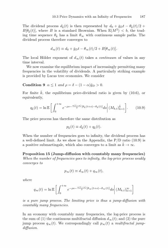
10.3 Price Dynamics with an Infinity of Frequencies 187

The dividend process dk(t) is then represented by d0 + gDt − θk(t)/2 +B[θk(t)], where B is a standard Brownian. When E(M2) < b, the trad-ing time sequence θk has a limit θ∞ with continuous sample paths. Thedividend process therefore converges to

d∞(t) ≡ d0 + gDt − θ∞(t)/2 + B[θ∞(t)].

The local Holder exponent of d∞(t) takes a continuum of values in anytime interval.

We now examine the equilibrium impact of increasingly permitting manyfrequencies in the volatility of dividends. A particularly striking exampleis provided by Lucas tree economies. We consider

Condition 9 α ≤ 1 and ρ = δ − (1 − α)gD > 0.

For finite k, the equilibrium price-dividend ratio is given by (10.6), orequivalently,

qk(t) = ln E

[∫ +∞

0e−ρs− α(1−α)

2 [θk(t+s)−θk(t)]ds

∣∣∣∣ (Mk,t)kk=1

]. (10.9)

The price process has therefore the same distribution as

pk(t) ≡ dk(t) + qk(t).

When the number of frequencies goes to infinity, the dividend process hasa well-defined limit. As we show in the Appendix, the P/D ratio (10.9) isa positive submartingale, which also converges to a limit as k → ∞.

Proposition 15 (Jump-diffusion with countably many frequencies)When the number of frequencies goes to infinity, the log-price process weaklyconverges to

p∞(t) ≡ d∞(t) + q∞(t),

where

q∞(t) = ln E

[∫ +∞

0e−ρs− α(1−α)

2 [θ∞(t+s)−θ∞(t)]ds

∣∣∣∣ (Mk,t)∞k=1

]

is a pure jump process. The limiting price is thus a jump-diffusion withcountably many frequencies.

In an economy with countably many frequencies, the log-price process isthe sum of (1) the continuous multifractal diffusion d∞(t); and (2) the purejump process q∞(t). We correspondingly call p∞(t) a multifractal jump-diffusion.

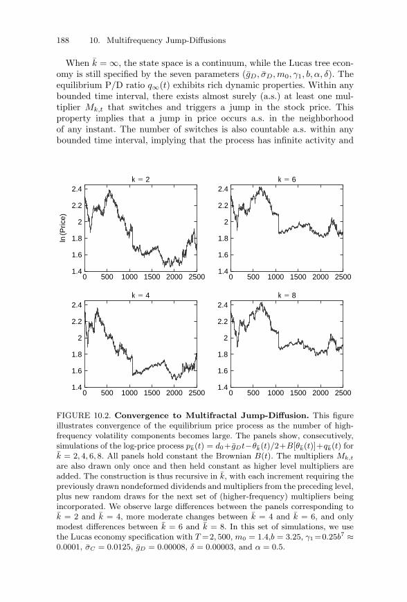
188 10. Multifrequency Jump-Diffusions

When k = ∞, the state space is a continuum, while the Lucas tree econ-omy is still specified by the seven parameters (gD, σD, m0, γ1, b, α, δ). Theequilibrium P/D ratio q∞(t) exhibits rich dynamic properties. Within anybounded time interval, there exists almost surely (a.s.) at least one mul-tiplier Mk,t that switches and triggers a jump in the stock price. Thisproperty implies that a jump in price occurs a.s. in the neighborhoodof any instant. The number of switches is also countable a.s. within anybounded time interval, implying that the process has infinite activity and

0 500 1000 1500 2000 25001.4

1.6

1.8

2

2.2

2.4k 5 2

ln(P

rice)

0 500 1000 1500 2000 25001.4

1.6

1.8

2

2.2

2.4k 5 6

1.4

1.6

1.8

2

2.2

2.4k 5 4

0 500 1000 1500 2000 25000 500 1000 1500 2000 25001.4

1.6

1.8

2

2.2

2.4k 5 8

FIGURE 10.2. Convergence to Multifractal Jump-Diffusion. This figureillustrates convergence of the equilibrium price process as the number of high-frequency volatility components becomes large. The panels show, consecutively,simulations of the log-price process pk(t) = d0+gDt−θk(t)/2+B[θk(t)]+qk(t) fork = 2, 4, 6, 8. All panels hold constant the Brownian B(t). The multipliers Mk,t

are also drawn only once and then held constant as higher level multipliers areadded. The construction is thus recursive in k, with each increment requiring thepreviously drawn nondeformed dividends and multipliers from the preceding level,plus new random draws for the next set of (higher-frequency) multipliers beingincorporated. We observe large differences between the panels corresponding tok = 2 and k = 4, more moderate changes between k = 4 and k = 6, and onlymodest differences between k = 6 and k = 8. In this set of simulations, we usethe Lucas economy specification with T =2, 500, m0 = 1.4,b = 3.25, γ1 =0.25b7 ≈0.0001, σC = 0.0125, gD = 0.00008, δ = 0.00003, and α = 0.5.

10.4 Recursive Utility and Priced Jumps 189

is continuous almost everywhere. Equilibrium valuation therefore generatesa limit P/D ratio that follows an infinite intensity pure jump process.

In Figure 10.2 we illustrate the convergence of the equilibrium priceprocesses as k becomes large. The first panel shows a simulation withk = 2 volatility components, and the following panels consecutively addhigher-frequency components to obtain paths with k = 4, k = 6, andk = 8 components. Consistent with the theoretical construction, the figureis obtained by randomly drawing a trajectory of the Brownian motion Bin stage k = 0, which is thereafter taken as fixed. Similarly, each multiplierMk,t is drawn only once, so that (Mk,t)k

k=1 does not vary when we movefrom stage k to stage k + 1. The figure suggests that the price processbecomes progressively insensitive to the addition of new high-frequencycomponents, and the sample path of the price process stabilizes. For low k,adding components has a significant impact, and as k increases the processconverges.

10.4 Recursive Utility and Priced Jumps

We showed in Chapter 9 that the equity premium can be matched with rea-sonable levels of risk aversion when investors have Epstein-Zin-Weil utilityand consumption undergoes regime switches. The recursive preference equi-librium easily generalizes to continuous time, permitting discontinuities inthe SDF and priced jumps, as we now show.

Agents have a stochastic differential utility Vt (Duffie and Epstein, 1992),which is specified by a normalized aggregator f(c, v) and satisfies the fixed-point equation

Vt = Et

[∫ T

t

f(Cs, Vs)ds + VT

](10.10)

for any instants T ≥ t ≥ 0. The aggregator is given by

f(c, v) ≡ δ

1 − ψ−1

c1−ψ−1 − [(1 − α)v]θ

[(1 − α)v]θ−1 ,

where α is the coefficient of relative risk aversion, ψ is the elasticity ofintertemporal substitution, and θ = (1 − ψ−1)/(1 − α). The case whereθ = 1 corresponds to isoelastic utility as considered previously.

Under the consumption process in Condition 7, the recursive utility hasfunctional form V (c, Mt) = ϕ(Mt)c1−α/(1 − α). 7 The stochastic discount

7The fixed-point equation (10.10) can be written as f(Ct, Vt)dt + Et(dVt) = 0.Let ϕ1, . . . , ϕd denote the value of ϕ in all possible states m1, . . . , md. The fixed-point

190 10. Multifrequency Jump-Diffusions

factor is then Λt = δ−1 exp[∫ t

0 fv(Cs, Vs)ds]fc(Ct, Vt) (Duffie and Epstein,

1992; Duffie and Skiadas, 1994), or equivalently

Λt = [ϕ(Mt)]1−θC−αt e− δ

θ t+δ(1− 1θ )

∫ t0 [ϕ(Ms)]−θds.

Consumption and the exponential expression are continuous. On the otherhand, the first factor in the equation is a function of ϕ(Mt), which dependson the Markov state and can therefore vary discontinuously throughtime. In the simplifying case where θ = 1 (power utility), the factor[ϕ(Mt)]1−θ drops out, and the SDF has continuous sample paths, reducingto Λt = e−δtC−α

t . On the other hand, if θ �= 1, the term [ϕ(Mt)]1−θ isdiscontinuous, and the marginal utility of consumption depends on thecurrent state. Discrete changes in the state vector Mt thus cause jumps inthe SDF.

Since switches in Mt trigger simultaneous jumps in the stochastic dis-count factor and the P/D ratio, they impact expected returns, and henceare“priced” in equilibrium. To see this, we denote by γ =

∑kk=1 γk the

intensity that at least one arrival occurs. Furthermore, let Et,A denote theexpectation operator conditional on (1) the investor information set It;and (2) the occurrence of at least one arrival between t and t + dt. Theconditional equity premium is then:

− 1dt

Et

(dΛt

Λt

dPt

Pt

)= ασC(Mt)σD(Mt)ρC,D + γEt,A

(−ΔΛt

Λt

ΔPt

Pt

).

When θ �= 1, the final term is generally nonzero, confirming that the possi-bility of a discontinuity modifies the expected return required by investorson the stock. Jumps represent a priced risk in equilibrium.

The ability of our framework to accommodate priced jumps is potentiallyuseful for empirical applications. For example, we have used nonseparablepreferences in Chapter 9 to obtain priced switches in a calibration thatsimultaneously fits, with reasonable levels of risk aversion, the equity pre-mium, equity volatility, and the drifts and volatilities of consumption anddividends. In a recent contribution, Bhamra, Kuehn, and Strebulaev (2006)extend this framework by considering levered claims on the priced asset.They find that the ability to capture priced jumps is empirically important

equation is then

δ

θ(ϕ1−θ

i − ϕi) + ϕi

[(1 − α)gC(mi) +

α(α − 1)2

σ2C(mi)

]+

∑j �=i

ai,j(ϕj − ϕi) = 0,

where ai,j = P(Mt+dt = mj |Mt = mi

)/dt. Existence and uniqueness can then be ana-

lyzed using standard methods.

10.5 Discussion 191

in simultaneously reconciling the equity premium, default spreads, andempirically observed default rates. We anticipate that future work will useour structural approach to modeling priced jumps in other applications,including, for example, pricing options and other derivatives.

10.5 Discussion

In this chapter, we develop a continuous-time asset pricing economy withendogenous multifrequency jumps in stock prices. Equilibrium valuationgives a number of appealing features that are often assumed exogenously inprevious literature, including: (1) heterogeneous jump sizes with many andfrequent small jumps and few large jumps; and (2) endogenous correlationbetween jumps in prices and volatility. Furthermore, jumps are priced inequilibrium under nonseparable preferences.

We consider the weak limit of our economic equilibrium as the num-ber of components driving fundamentals becomes large. Under appropriateconditions, the stock price converges to a new mathematical object calleda multifractal jump-diffusion. The equity value can be decomposed intothe continuous multifractal diffusion followed by the exogenous dividendprocess, and an infinite-intensity pure jump process corresponding toendogenous variations in the price-dividend ratio.

The chapter can be viewed as bridging a gap between exogenouslyspecified jump-diffusions and discrete-time equilibrium models of volatil-ity feedback, such as in Chapter 9. More generally, the model illustratesthat equilibrium is a powerful method to generate endogenous pricediscontinuities in financial economics.

11Conclusion

The Markov-switching approach to multifractal modeling offers aparsimonious and accurate statistical description of financial time seriesbased on the concept of scale-invariant multifrequency risk. In the mostbasic construction, MSM is driven by a Markov state vector with multiplecomponents, whose rescaled product defines total volatility. Each of thecomponents, or multipliers, can switch to a new level with a different prob-ability per unit time, generating volatility shocks of multiple frequencies.When an arrival does occur in a given multiplier, a new value is drawnfrom a fixed distribution independently of all other variables in the model.The marginal distributions of all volatility components are hence identical,which provides parsimony to MSM and finds empirical support at stan-dard confidence levels. The construction works equally well in discrete andcontinuous time, and easily extends to multivariate settings.

From a statistical point of view, elaborated in Parts I and II of thebook, MSM captures thick tails, long-memory features, and intertwinedvolatility cycles of heterogeneous durations. When volatility componentshave a discrete distribution, MSM is a latent Markov chain, and its para-meters can be estimated by maximizing the closed-form likelihood of thereturn series. Alternatively, return moments can be used to quickly cali-brate or estimate MSM. Once the parameters have been imputed, theapplied researcher can readily compute the conditional distribution of thevolatility state and returns at any instant. Bayesian updating permits filter-ing of volatility components, and the Markov construction implies tractablemultistep prediction. The research presented in this book and subsequentstudies have shown that MSM performs well in-sample, produces goodforecasts of volatility, and generates reliable estimates of the value-at-riskin a position or portfolio of assets.

MSM also captures the unconditional moments of returns, and in particu-lar the “power variations” of many financial series, which have been studiedextensively (e.g., Andersen et al., 2001; Barndorff-Nielsen and Shephard,2003; Calvet and Fisher, 2002a; Calvet, Fisher, and Mandelbrot, 1997;Galluccio et al., 1997; Ghashghaie et al., 1996; Pasquini and Serva, 1999,2000; Richards, 2000; Vandewalle and Ausloos, 1998; Vassilicos, Demos,and Tata, 1993). The multifractal model implies that the qth moment ofabsolute returns scales as a power function of the frequency of observation,

194 11. Conclusion

provided that the qth moment exists. Furthermore, across q the scalingexponents used in the power functions form a nonlinear strictly convex func-tion of q. Extensive research, including results presented in this book, showsthat these scaling properties hold in a variety of currency and equity series.

The transition between discrete- and continuous-time versions of MSM isremarkably straightforward, which is a substantial operational advantageof our approach. Additional insights can be gained from continuous-timeMSM by considering the limit time deformation when the number of high-frequency components goes to infinity. Because local volatility exhibitsincreasingly extreme fluctuations, the Lebesgue dominated convergencetheorem does not apply and in fact gives the misleading intuition that thelimit trading time converges to zero. By contrast, a correct analysis usingthe martingale convergence theorem and appropriate tightness conditionsimplies that the trading-time sequence converges to a nondegenerate timedeformation process. The limiting multifractal diffusion is driven by count-ably many components, and its sample paths contain a continuum of localHolder exponents in any time interval.

In Part III we show that MSM integrates easily into equilibrium models,providing a tractable framework within which to analyze the impact ofmultifrequency shocks on endogenous asset prices. We consider a con-sumption-based economy as in Lucas (1978) with MSM shocks to dividendnews, and in some cases, consumption growth. The presence of volatilityshocks of heterogeneous durations generates endogenous variations in theprice-dividend ratio, and the volatility of returns can be substantially higherthan the volatility of dividends. Investor learning endogenously generatesnegative skewness in stock returns because increases in volatility (bad news)tend to be revealed abruptly while decreases in volatility (good news) arelikely to be inferred gradually. Long-run risk is naturally present in MSM,and helps to generate equilibrium stock returns consistent with the equitypremium. In continuous time, volatility shocks of heterogeneous dura-tions lead to endogenous jumps in prices, with many small discontinuities,frequent moderate jumps, and rare extreme events. As the number ofvolatility components diverges to infinity, the continuous-time equilibriumapproach generates a new mathematical object, which is the sum ofa continuous multifractal diffusion and an infinite intensity pure jumpprocess. We call this new process a multifractal jump-diffusion.

Numerous applications, extensions, and research questions emerge natu-rally from the research developed in this book. For example, practitionersinterested in the implementation of MSM on real-time data can imputethe parameters of MSM by either maximizing the closed-form likelihood orusing a moment-based calibration, as illustrated in Chapter 8. The inferreddata generating process can be used to forecast volatility or produceestimates of value-at-risk. Lux (2008) provides additional discussion of sim-plified estimation and forecasting methods. Practitioners may also seekto use MSM to price options, for instance by considering multifrequency

11. Conclusion 195

variants of the Hull and White (1987) model. In ongoing research, we havefound evidence that MSM can be very helpful in pricing options and otherderivatives. We anticipate that applications of multifractals to derivativesvaluation will be a growth area in coming years.

Econometricians may be interested in further expanding and developingapplications of fractal-type methods. MSM illustrates that pure regime-switching models can match and in some cases outperform smoothlyautoregressive volatility processes. As suggested by Hamilton (2006), thegeneral approach of investigating high-dimensional but parsimonious andstructured regime-switching offers considerable promise and will likelyreceive further attention.

Theoretical researchers can use the models in this book to reexaminethe common view that wild fluctuations in financial markets are incon-sistent with the concept of economic equilibrium (e.g., Mandelbrot andHudson, 2004). As pointed out by Bansal and Yaron (2004), risk premiacan be high and returns volatile in a world where fundamentals are verypersistent. MSM equilibrium models accommodate these low-frequency fea-tures, while simultaneously providing sufficient realism at high frequenciesthat the model can be estimated using maximum likelihood on daily data.Through this approach, we are able to bring together aspects of both thehigh-frequency financial econometrics and lower-frequency macro-financeliteratures.

Recent literature in financial economics and asset management has gen-erated renewed interest in the modeling and pricing implications of rareevents (e.g., Barro, 2006; Taleb, 2007). MSM provides new insights onhow these risks can be specified and are likely to affect asset prices. Todevelop intuition, one can begin by considering a single-frequency MSMspecification with a very low value of γ1. Changes in the drift or volatil-ity of fundamentals are very rare, but produce extreme asset returns inequilibrium when they do occur. Estimation is course difficult in such anenvironment, as it is effectively based on very few observations or perhapsnone at all.

The multifractal setting implies that rare events need not be studied inisolation. In particular, the structure imposed by MSM, which appears tobe consistent with empirical evidence, suggests that variations at high andmedium frequencies may help to build a reasonable framework for lower-frequency events. From an intuitive point of view, gradations in size andfrequency exist even in the context of disaster, depression, and war, andmodels assuming a dichotomy between normal and catastrophic states canmiss such regularities. Furthermore given an existing MSM specification,one can easily contemplate adding in additional possibilities for rare eventsby either lowering the intensity of arrival γ1 of the most persistent compo-nent, or equivalently by assuming that some component of arrival intensityγ0 = γ1/b has not switched during recorded history. The structure of MSMallows the applied researcher to infer the likely size and price impact of

196 11. Conclusion

such shocks, and thus stress-test pricing and risk management models.The recent turbulence in the financial markets highlights the usefulnessof considering shocks larger than those that have been hitherto observed.

MSM offers the finance profession an opportunity to tie together variousphenomena that have been previously modeled in isolation. The interac-tion of shocks with heterogeneous frequencies is a potent source of pricedynamics that can explain financial data at all horizons with a very limi-ted number of parameters. We anticipate that future research will furtherdemonstrate the validity of this approach.

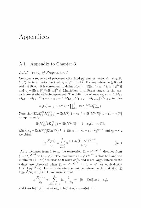
AAppendices

A.1 Appendix to Chapter 3

A.1.1 Proof of Proposition 1Consider a sequence of processes with fixed parameter vector ψ = (m0, σ,b, γ∗). Note in particular that γk = γ∗ for all k. For any integer n ≥ 0 andreal q ∈ [0,∞), it is convenient to define Kq(n) = E(|rt|q |rt+n|q)/[E(|rt|2q)]and cq = [E(|εt|q)]2/[E(|εt|2q)]. Multipliers in different stages of the cas-cade are statistically independent. The definition of returns, rt = σ(M1,t

M2,t . . . Mk,t)1/2εt and rt+n = σ(M1,t+nM2,t+n . . . Mk,t+n)1/2εt+n, implies

Kq(n) = cq[E(Mq)]−k∏k

k=1E(Mq/2

k,t Mq/2k,t+n).

Note that E(Mq/2k,t M

q/2k,t+n) = E(Mq)(1 − γk)n + [E(Mq/2)]2[1 − (1 − γk)n]

or equivalently

E(Mq/2k,t M

q/2k,t+n) = [E(Mq/2)]2 [1 + aq(1 − γk)n],

where aq = E(Mq)/[E(Mq/2)]2−1. Since 1 − γk = (1−γk)bk−k

and γk = γ∗,we obtain

lnKq(n)

cq=

k∑

k=1

ln1 + aq(1 − γ∗)nbk−k

1 + aq. (A.1)

As k increases from 1 to k, the expression (1 − γ∗)nbk−k

declines from(1−γ∗)nb1−k

to (1−γ∗)n. The maximum (1−γ∗)nb1−k

is close to 1 and theminimum (1 − γ∗)n is close to 0 when bk/n and n are large. Intermediatevalues are observed when (1 − γ∗)nbk−k ≈ 1 − γ∗, or equivalentlyk ≈ logb(bk/n). Let i(n) denote the unique integer such that i(n) ≤logb(bk/n) < i(n) + 1. We surmise that

lnKq(n)

cq≈

k∑

k=i(n)+1

ln1

1 + aq= −[k − i(n)] ln(1 + aq),

and thus ln [Kq(n)] ≈ −(logb n) ln(1 + aq) = −δ(q) ln n.

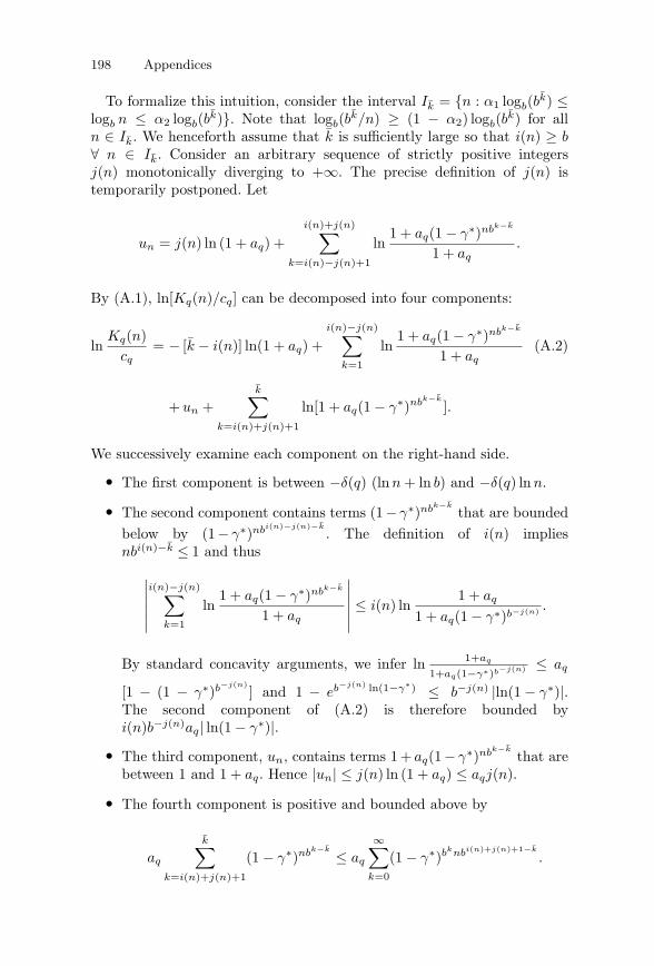
198 Appendices

To formalize this intuition, consider the interval Ik = {n : α1 logb(bk) ≤logb n ≤ α2 logb(bk)}. Note that logb(bk/n) ≥ (1 − α2) logb(bk) for alln ∈ Ik. We henceforth assume that k is sufficiently large so that i(n) ≥ b∀ n ∈ Ik. Consider an arbitrary sequence of strictly positive integersj(n) monotonically diverging to +∞. The precise definition of j(n) istemporarily postponed. Let

un = j(n) ln (1 + aq) +i(n)+j(n)∑

k=i(n)−j(n)+1

ln1 + aq(1 − γ∗)nbk−k

1 + aq.

By (A.1), ln[Kq(n)/cq] can be decomposed into four components:

lnKq(n)

cq= − [k − i(n)] ln(1 + aq) +

i(n)−j(n)∑

k=1

ln1 + aq(1 − γ∗)nbk−k

1 + aq(A.2)

+un +k∑

k=i(n)+j(n)+1

ln[1 + aq(1 − γ∗)nbk−k

].

We successively examine each component on the right-hand side.

• The first component is between −δ(q) (lnn + ln b) and −δ(q) ln n.

• The second component contains terms (1− γ∗)nbk−k

that are boundedbelow by (1− γ∗)nbi(n)−j(n)−k

. The definition of i(n) impliesnbi(n)−k ≤ 1 and thus

∣∣∣∣∣∣

i(n)−j(n)∑

k=1

ln1 + aq(1 − γ∗)nbk−k

1 + aq

∣∣∣∣∣∣≤ i(n) ln

1 + aq

1 + aq(1 − γ∗)b−j(n) .

By standard concavity arguments, we infer ln 1+aq

1+aq(1−γ∗)b−j(n) ≤ aq

[1 − (1 − γ∗)b−j(n)] and 1 − eb−j(n) ln(1−γ∗) ≤ b−j(n) |ln(1 − γ∗)|.

The second component of (A.2) is therefore bounded byi(n)b−j(n)aq| ln(1 − γ∗)|.

• The third component, un, contains terms 1 + aq(1 − γ∗)nbk−k

that arebetween 1 and 1 + aq. Hence |un| ≤ j(n) ln (1 + aq) ≤ aqj(n).

• The fourth component is positive and bounded above by

aq

k∑

k=i(n)+j(n)+1

(1 − γ∗)nbk−k ≤ aq

∞∑

k=0

(1 − γ∗)bknbi(n)+j(n)+1−k

.

A.1 Appendix to Chapter 3 199

We check that nbi(n)+j(n)+1−k ≥ 1 and bk ≥ k(b − 1). The fourthcomponent is therefore bounded above by aq

∑∞k=0(1 − γ∗)k(b−1) =

aq

1−(1−γ∗)b−1 .

This establishes that

∣∣∣∣lnKq(n)lnn−δ(q) − 1

∣∣∣∣ ≤c∗q + aqj(n) + aqi(n)b−j(n)| ln(1 − γ∗)|

δ(q) ln n,

where c∗q = δ(q) ln b + | ln cq| + aq/[1 − (1 − γ∗)(b−1)]. We now choose a

sequence j(n) such that the right-hand side of the inequality convergesto 0. More specifically, consider the unique integer such that1 j(n) ≤2 logb i(n) < j(n)+1. It is easy to check that i(n)b−j(n) = blogb i(n)−j(n) ≤ 1and j(n) ≤ 2 logb k. For all n ∈ Ik, the quantity

∣∣∣ ln Kq(n)ln n−δ(q) − 1

∣∣∣ is thereforebounded above by

ηk =1

k δ(q)α1 ln b

[2aq logb k + c∗

q + aq| ln(1 − γ∗)|], (A.3)

which is independent of n. We infer that supn∈Ik

∣∣∣ ln Kq(n)ln n−δ(q) − 1

∣∣∣ → 0 as

k → +∞.Finally, we observe that

∣∣∣∣ln ρq(n)lnn−δ(q) − 1

∣∣∣∣ ≤∣∣∣∣logb [ρq(n)/Kq(n)]

lnn−δ(q)

∣∣∣∣+∣∣∣∣lnKq(n)lnn−δ(q) − 1

∣∣∣∣.

The autocorrelation ρq(n) satisfies

1 ≤ Kq(n)ρq(n)

=1 − cq(1 + aq)−k

1 − cq(1 + aq)−k/Kq(n)≤ 1

1 − cq(1 + aq)−k/Kq(n). (A.4)

Equation (A.3) implies that for all n ∈ Ik, logb Kq(n) ≥ −δ(q)(1 + ηk)α2k,and thus

logb[Kq(n)/(1 + aq)−k] ≥ kδ(q)(1 − α2 − α2ηk). (A.5)

Combining (A.4) and (A.5), we conclude that supn∈Ik

∣∣∣ln Kq(n)ρq(n)

∣∣∣ → 0 andthat the Proposition holds.

1We check that when k is large enough, 1 ≤ j(n) ≤ i(n) and j(n) + i(n) ≤ k for

all n ∈ Ik.

200 Appendices

A.1.2 HAC-Adjusted Vuong TestWe consider the probability space (Ω,F , P0) and a stochastic process{rt}+∞

t=1 . Each rt is a random variable taking values on the real line. Forevery t, it is convenient to consider the vector of past values Rt−1 ={rs}t−1

s=1. The econometrician directly observes a finite number of reali-zations of rt but does not know the true data-generating process. Sheinstead considers two competing families of models specified by their condi-tional densities Mf = {f(rt|Rt−1, θ); θ ∈ Θ} and Mg = {g(rt|Rt−1, γ); γ ∈Γ}. These families may or may not contain the true data-generating pro-cess. The pseudo true value θ∗ specifies the model in Mf with the optimalKullback-Leibler Information Criterion:

θ∗ = arg maxθ∈Θ

E0[ln f(rt|Rt−1, θ)].

The pseudo true value γ∗ is similarly defined.Consider the log-likelihood functions:

LfT (θ) ≡

T∑

t=1

ln f(rt|Rt−1, θ), LgT (γ) ≡

T∑

t=1

ln g(rt|Rt−1, γ).

By definition, the ML estimators θT and γT maximize the functions LfT (θ)

and LgT (γ). The corresponding first-order conditions are

∂LfT

∂θ(θT ) = 0,

∂LgT

∂θ(γT ) = 0. (A.6)

We now examine the likelihood ratio

LRT (θT , γT ) = LfT (θT ) − Lg

T (γT ) =T∑

t=1

lnf(rt|Rt−1, θT )g(rt|Rt−1, γT )

.

By Equation (A.6), a second-order expansion of LRT implies that1√T

LRT (θT , γT ) = 1√T

LRT (θ∗, γ∗) + op(1), and thus

1√T

LRT (θT , γT ) =1√T

T∑

t=1

lnf(rt|Rt−1, θ

∗)g(rt|Rt−1, γ∗)

+ op(1).

Let at = ln[f(rt|Rt−1, θ∗)/g(rt|Rt−1, γ

∗)] and at = ln[f(rt|Rt−1, θT )/g(rt|Rt−1, γT )].

When the observations rt are i.i.d., the addends at are also i.i.d..If the models f and g have equal Kullback-Leibler Information crite-rion, the central limit theorem implies T−1/2LRT (θT , γT ) d→ N (0, σ2

∗),

A.2 Appendix to Chapter 4 201

where σ2∗ = V ar(at). The variance is consistently estimated by the sample

variance of {at}.In the non-i.i.d. case, we need to adjust for the correlation in the addends

at. Let σ2T = T−1∑T

s=1∑T

t=1 E(asat). We know that T−1/2LRT (θT , γT ) =σT Z + op(1), where Z is a standard Gaussian. Following Newey-West(1987), we estimate σT by

σ2T = Ω0 + 2

m∑

j=1

w(j, m)Ωj ,

where Ωj =∑T

t=j+1 atat−j/T denotes the sample covariance of {at}, andw(j, m) = 1 − j/(m + 1) is the Bartlett weight. We choose m using theautomatic lag selection method of Newey and West (1994).

A.2 Appendix to Chapter 4

A.2.1 Distribution of the Arrival VectorThe probability of a simultaneous switch is P(1α

k,t = 1βk,t = 1) = P(1α

k,t = 1)P(1β

k,t = 1|1αk,t = 1). The vector 1k,t therefore has unconditional distri-

bution:

Arrival on β No arrival on β

Arrival on α γk[(1 − λ)γk + λ] γk(1 − λ)(1 − γk)No arrival on α γk(1 − γk)(1 − λ) (1 − γk)[1 − γk(1 − λ)].

A.2.2 Ergodic Distribution of Volatility ComponentsThe bivariate process (Mα

k,t, Mβk,t) can take values s1 = sH,H = (mα

0 , mβ0 ),

s2 = sH,L = (mα0 , mβ

1 ), s3 = sL,H = (mα1 , mβ

0 ) and s4 = sL,L = (mα1 , mβ

1 ).The transition matrix is T = (tij), where tij = P(st+1 = sj |st = si). Itsatisfies

T =

⎡

⎢⎢⎢⎣

pk 1 − γk

2 − pk 1 − γk

2 − pk γk − 1 + pk

1 − γk

2 − qk qk γk − 1 + qk 1 − γk

2 − qk

1 − γk

2 − qk γk − 1 + qk qk 1 − γk

2 − qk

γk − 1 + pk 1 − γk

2 − pk 1 − γk

2 − pk pk

⎤

⎥⎥⎥⎦,

where

pk = 1 − γk + γk[(1 − λ)γk + λ]1 + ρ∗

m

4,

qk = 1 − γk + γk[(1 − λ)γk + λ]1 − ρ∗

m

4.

202 Appendices

Simple manipulation implies that the characteristic polynomial of T is

PT (x) = (1 − x)(1 − γk − x)2[2(pk + qk + γk) − 3 − x].

We easily check that |2(pk + qk + γk) − 3| < 1, and we infer that T has aunique ergodic distribution Πk = (ΠHH

k , ΠHLk , ΠLH

k , ΠLLk ). The symmetry

of the transition matrix implies that ΠHHk = ΠLL

k and ΠHLk = ΠLH

k . Weeasily check that ΠHH

k = 14

2−2qk−γk

2−(pk+qk)−γk, or equivalently

ΠHHk =

14

1 − (1 − ρ∗m)[(1 − λ)γk + λ]/2

1 − [(1 − λ)γk + λ]/2,

and finally note that ΠHLk = 1/2 − ΠHH

k . When ρ∗m > 0, the multipliers

are more likely to be either both high or both low: ΠHHk = ΠLL

k > 1/4 >ΠHL

k = ΠLHk .

A.2.3 Particle FilterAs discussed in the main text, the vectors M

(1)t+1, . . . , M

(B)t+1 are independent

draws from the probability distribution h(m) ≡ P(Mt+1 = m|Rt). Considera continuous function Y defined on R

k+ and taking values on the real

line. The conditional expectation E [Y (Mt+1)|Rt+1] =∑d

j=1 P(Mt+1 =mj |Rt+1) Y (mj) is conveniently rewritten as

E [Y (Mt+1)|Rt+1] =d∑

j=1

h(mj)P(Mt+1 = mj |Rt+1)

h(mj)Y (mj) .

The Monte Carlo approximation to this integral is

E [Y (Mt+1)|Rt+1] ≈ 1B

B∑

b=1

P(Mt+1 = M(b)t+1|Rt+1)

h(M (b)t+1)

Y (M (b)t+1).

Bayes’ rule implies

P(Mt+1 = M(b)t+1|Rt+1)

B h(M (b)t+1)

=frt+1(rt+1|Mt+1 = M

(b)t+1)

B frt+1 (rt+1|Rt).

Since frt+1 (rt+1|Rt) ≈ 1B

∑Bb′=1 frt+1(rt+1|M (b′)

t+1), we infer that

P(Mt+1 = M(b)t+1|Rt+1)

B h(M (b)t+1)

≈frt+1(rt+1|Mt+1 = M

(b)t+1)∑B

b′=1 frt+1(rt+1|Mt+1 = M(b′)t+1)

.

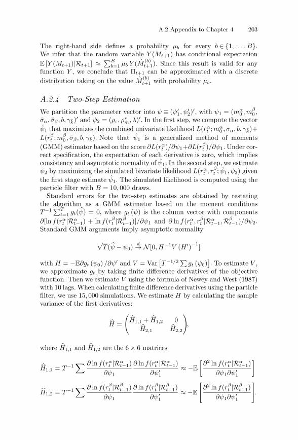
A.2 Appendix to Chapter 4 203

The right-hand side defines a probability μb for every b ∈ {1, . . . , B}.We infer that the random variable Y (Mt+1) has conditional expectationE [Y (Mt+1)|Rt+1] ≈

∑Bb=1 μb Y (M (b)

t+1). Since this result is valid for anyfunction Y , we conclude that Πt+1 can be approximated with a discretedistribution taking on the value M

(b)t+1 with probability μb.

A.2.4 Two-Step EstimationWe partition the parameter vector into ψ ≡ (ψ′

1, ψ′2)

′, with ψ1 = (mα0 , mβ

0 ,σα, σβ , b, γk)′ and ψ2 = (ρε, ρ

∗m, λ)′. In the first step, we compute the vector

ψ1 that maximizes the combined univariate likelihood L(rαt ;mα

0 , σα, b, γk)+L(rβ

t ;mβ0 , σβ , b, γk). Note that ψ1 is a generalized method of moments

(GMM) estimator based on the score ∂L(rαt )/∂ψ1+∂L(rβ

t )/∂ψ1. Under cor-rect specification, the expectation of each derivative is zero, which impliesconsistency and asymptotic normality of ψ1. In the second step, we estimateψ2 by maximizing the simulated bivariate likelihood L(rα

t , rβt ; ψ1, ψ2) given

the first stage estimate ψ1. The simulated likelihood is computed using theparticle filter with B = 10, 000 draws.

Standard errors for the two-step estimates are obtained by restatingthe algorithm as a GMM estimator based on the moment conditionsT−1∑T

t=1 gt(ψ) = 0, where gt (ψ) is the column vector with components∂[ln f(rα

t |Rαt−1) + ln f(rβ

t |Rβt−1)]/∂ψ1 and ∂ ln f(rα

t , rβt |Rα

t−1,Rβt−1)/∂ψ2.

Standard GMM arguments imply asymptotic normality

√T (ψ − ψ0)

d→ N [0, H−1V (H ′)−1]

with H = −E∂gt (ψ0) /∂ψ′ and V = Var[T−1/2∑ gt (ψ0)

]. To estimate V ,

we approximate gt by taking finite difference derivatives of the objectivefunction. Then we estimate V using the formula of Newey and West (1987)with 10 lags. When calculating finite difference derivatives using the particlefilter, we use 15, 000 simulations. We estimate H by calculating the samplevariance of the first derivatives:

H =

(H1,1 + H1,2 0

H2,1 H2,2

),

where H1,1 and H1,2 are the 6 × 6 matrices

H1,1 = T−1∑ ∂ ln f(rα

t |Rαt−1)

∂ψ1

∂ ln f(rαt |Rα

t−1)∂ψ′

1≈ −E

[∂2 ln f(rα

t |Rαt−1)

∂ψ1∂ψ′1

]

H1,2 = T−1∑ ∂ ln f(rβ

t |Rβt−1)

∂ψ1

∂ ln f(rβt |Rβ

t−1)∂ψ′

1≈ −E

[∂2 ln f(rβ

t |Rβt−1)

∂ψ1∂ψ′1

].

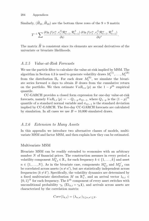
204 Appendices

Similarly, (H21, H22) are the bottom three rows of the 9 × 9 matrix

T−1∑ ∂ ln f(rα

t , rβt |Rα

t−1,Rβt−1)

∂ψ

∂ ln f(rαt , rβ

t |Rαt−1,R

βt−1)

∂ψ′ .

The matrix H is consistent since its elements are second derivatives of theunivariate or bivariate likelihoods.

A.2.5 Value-at-Risk ForecastsWe use the particle filter to calculate the value-at-risk implied by MSM. Thealgorithm in Section 4.3 is used to generate volatility draws M

(1)t , . . . , M

(B)t

from the distribution Πt. For each draw M(b)t , we simulate the bivari-

ate series forward n days to obtain B draws from the cumulative returnon the portfolio. We then estimate V aRt,n (p) as the 1 − pth empiricalquantile.

CC-GARCH provides a closed form expression for one-day value-at-riskforecasts, namely V aRt,1 (p) = − Q1−p σt|t−1, where Q1−p is the (1 − p)th

quantile of a standard normal variable and σt|t−1 is the standard deviationimplied by CC-GARCH. The five-day CC-GARCH forecasts are calculatedby simulation. In all cases we use B = 10,000 simulated draws.

A.2.6 Extension to Many AssetsIn this appendix we introduce two alternative classes of models, multi-variate MSM and factor MSM, and then explain how they can be estimated.

Multivariate MSM

Bivariate MSM can be readily extended to economies with an arbitrarynumber N of financial prices. The construction assumes in every period avolatility component Mn

k,t ∈ R+ for each frequency k ∈ {1, . . . , k} and assetn ∈ {1, . . . , N}. As in the bivariate case, components Mn

k,t and Mn′

k′,t canbe correlated across assets (n �=n′), but are statistically independent acrossfrequencies (k �= k′). Specifically, the volatility dynamics are determined bya fixed multivariate distribution M on R

N+ , and an arrival vector 1k,t ∈

{0, 1}N for each frequency. The kth component of every asset switches withunconditional probability γk (E1k,t = γk1), and arrivals across assets arecharacterized by the correlation matrix:

Corr(1k,t) = (λn,n′)1≤n,n′≤N .

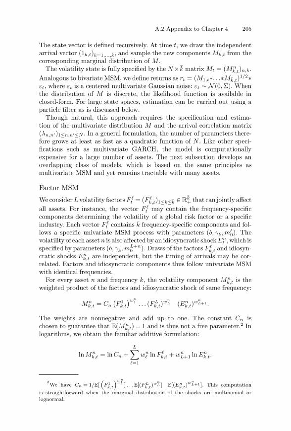
A.2 Appendix to Chapter 4 205

The state vector is defined recursively. At time t, we draw the independentarrival vector (1k,t)k=1,...,k, and sample the new components Mk,t from thecorresponding marginal distribution of M .

The volatility state is fully specified by the N × k matrix Mt = (Mnk,t)n,k.

Analogous to bivariate MSM, we define returns as rt = (M1,t∗. . .∗Mk,t)1/2∗εt, where εt is a centered multivariate Gaussian noise: εt ∼ N (0,Σ). Whenthe distribution of M is discrete, the likelihood function is available inclosed-form. For large state spaces, estimation can be carried out using aparticle filter as is discussed below.

Though natural, this approach requires the specification and estima-tion of the multivariate distribution M and the arrival correlation matrix(λn,n′)1≤n,n′≤N . In a general formulation, the number of parameters there-fore grows at least as fast as a quadratic function of N . Like other speci-fications such as multivariate GARCH, the model is computationallyexpensive for a large number of assets. The next subsection develops anoverlapping class of models, which is based on the same principles asmultivariate MSM and yet remains tractable with many assets.

Factor MSM

We consider L volatility factors F t = (F

k,t)1≤k≤k ∈ Rk+ that can jointly affect

all assets. For instance, the vector F t may contain the frequency-specific

components determining the volatility of a global risk factor or a specificindustry. Each vector F

t contains k frequency-specific components and fol-lows a specific univariate MSM process with parameters (b, γk, m

0). Thevolatility of each asset n is also affected by an idiosyncratic shock En

t , which isspecified by parameters (b, γk, mL+n

0 ). Draws of the factors F k,t and idiosyn-

cratic shocks Enk,t are independent, but the timing of arrivals may be cor-

related. Factors and idiosyncratic components thus follow univariate MSMwith identical frequencies.

For every asset n and frequency k, the volatility component Mnk,t is the

weighted product of the factors and idiosyncratic shock of same frequency:

Mnk,t = Cn

(F 1

k,t

)wn1 . . . (FL

k,t)wn

L (Enk,t)

wnL+1 .

The weights are nonnegative and add up to one. The constant Cn ischosen to guarantee that E(Mn

k,t) = 1 and is thus not a free parameter.2 Inlogarithms, we obtain the familiar additive formulation:

lnMnk,t = ln Cn +

L∑

=1

wn lnF

k,t + wnL+1 lnEn

k,t.

2We have Cn = 1/E[

(F 1

k,t

)wn1 ] . . . E[(F L

k,t)wn

L ] E[(Enk,t)

wnL+1 ]. This computation

is straightforward when the marginal distribution of the shocks are multinomial orlognormal.

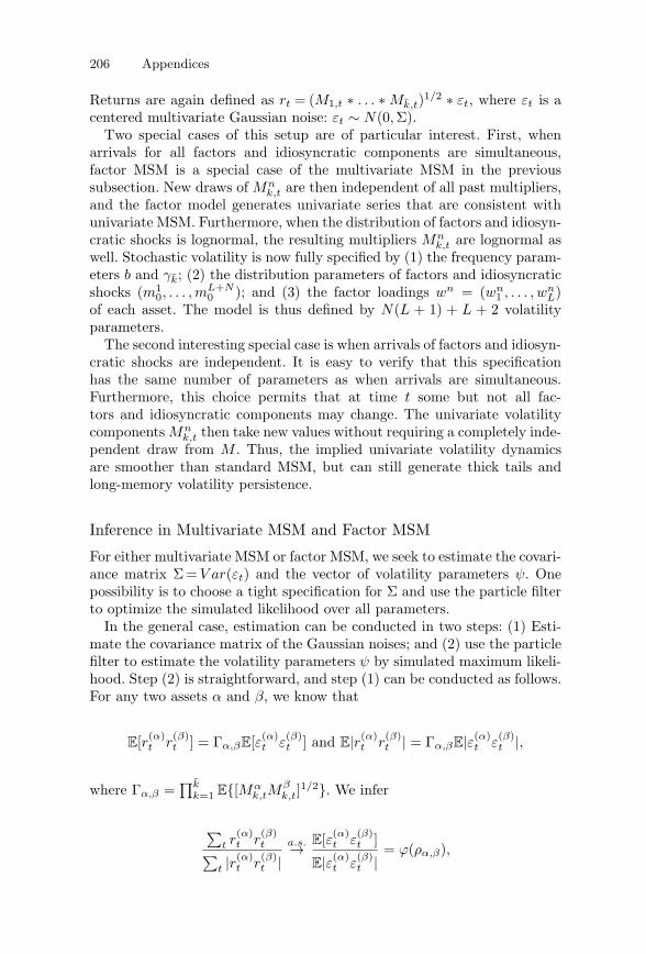
206 Appendices

Returns are again defined as rt = (M1,t ∗ . . . ∗ Mk,t)1/2 ∗ εt, where εt is acentered multivariate Gaussian noise: εt ∼ N(0,Σ).

Two special cases of this setup are of particular interest. First, whenarrivals for all factors and idiosyncratic components are simultaneous,factor MSM is a special case of the multivariate MSM in the previoussubsection. New draws of Mn

k,t are then independent of all past multipliers,and the factor model generates univariate series that are consistent withunivariate MSM. Furthermore, when the distribution of factors and idiosyn-cratic shocks is lognormal, the resulting multipliers Mn

k,t are lognormal aswell. Stochastic volatility is now fully specified by (1) the frequency param-eters b and γk; (2) the distribution parameters of factors and idiosyncraticshocks (m1

0, . . . , mL+N0 ); and (3) the factor loadings wn = (wn

1 , . . . , wnL)

of each asset. The model is thus defined by N(L + 1) + L + 2 volatilityparameters.

The second interesting special case is when arrivals of factors and idiosyn-cratic shocks are independent. It is easy to verify that this specificationhas the same number of parameters as when arrivals are simultaneous.Furthermore, this choice permits that at time t some but not all fac-tors and idiosyncratic components may change. The univariate volatilitycomponents Mn

k,t then take new values without requiring a completely inde-pendent draw from M . Thus, the implied univariate volatility dynamicsare smoother than standard MSM, but can still generate thick tails andlong-memory volatility persistence.

Inference in Multivariate MSM and Factor MSM

For either multivariate MSM or factor MSM, we seek to estimate the covari-ance matrix Σ = V ar(εt) and the vector of volatility parameters ψ. Onepossibility is to choose a tight specification for Σ and use the particle filterto optimize the simulated likelihood over all parameters.

In the general case, estimation can be conducted in two steps: (1) Esti-mate the covariance matrix of the Gaussian noises; and (2) use the particlefilter to estimate the volatility parameters ψ by simulated maximum likeli-hood. Step (2) is straightforward, and step (1) can be conducted as follows.For any two assets α and β, we know that

E[r(α)t r

(β)t ] = Γα,βE[ε(α)

t ε(β)t ] and E|r(α)

t r(β)t | = Γα,βE|ε(α)

t ε(β)t |,

where Γα,β =∏k

k=1 E{[Mαk,tM

βk,t]

1/2}. We infer

∑t r

(α)t r

(β)t∑

t |r(α)t r

(β)t |

a.s.→ E[ε(α)t ε

(β)t ]

E|ε(α)t ε

(β)t |

= ϕ(ρα,β),

A.3 Appendix to Chapter 5 207

where ρα,β = Corr[ε(α)t ; ε(β)

t ] and ϕ(ρ) ≡ π2

ρ√1−ρ2+ρ arcsin ρ

. The function ϕ

is strictly increasing and maps [−1, 1] onto [−1, 1]. A consistent estimatorof the correlation coefficient is therefore

ρα,β = ϕ−1

( ∑t r

(α)t r

(β)t∑

t |r(α)t r

(β)t |

).

The variance of the Gaussians is consistently estimated by σ2α =

1T

∑t[r

(α)t ]2. Since the covariance matrix defined by the above estimates

may not be positive definite, we then apply the methodology of Ledoit,Santa-Clara, and Wolf (2003) to obtain a positive semidefinite matrix Σ.

A.3 Appendix to Chapter 5

A.3.1 Properties of DConsider a fixed instant t ∈ [0, 1]. For all ε > 0, there exists a dyadic numbertn such that |tn − t| < ε. We can then find a number Δn = b−kn < ε forwhich (tn,Δn) ∈ D. In the plane R

2, the point (t, 0) is thus the limit of thesequence (tn,Δn) ∈ D. This establishes that the closure of D contains theset [0, 1] × {0}. The scaling relation (5.4) thus holds “in the neighborhoodof any instant.”

A.3.2 Interpretation of f(α) as a Fractal DimensionFractal geometry considers irregular and winding structures that are notwell described by their Euclidean length. For instance, a geographer mea-suring the length of a coastline will find very different results as sheincreases the precision of her measurement. In fact, the structure of thecoastline is usually so intricate that the measured length diverges to infin-ity as the geographer’s measurement scale goes to zero. For this reason,it is natural to introduce a new concept of dimension (Mandelbrot 1982).Given a precision level ε > 0, we consider coverings of the coastline withballs of diameter ε. Let N(ε) denote the smallest number of balls requiredfor such a covering. The approximate length of the coastline is defined byL(ε) = εN(ε). In many cases, N(ε) satisfies a power law as ε goes to zero:

N(ε) ∼ ε−D,

where D is a constant called the fractal dimension.Fractal dimension helps to analyze the structure of a fixed multifractal.

For any α ≥ 0, we can define the set T (α) of instants with Holder exponentα. As any subset of the real line, T (α) has a fractal dimension D(α), whichsatisfies 0 ≤D(α) ≤ 1. For a large class of multifractals, the dimension D(α)

208 Appendices

coincides with the multifractal spectrum f(α) (Frisch and Parisi, 1985;Halsey et al., 1986; Peyriere 1991).

In the case of measures, we can provide a heuristic interpretation ofthis result based on coarse Holder exponents. Denoting by N(α, Δt) thenumber of intervals [t, t + Δt] required to cover T (α), we infer fromEquation (5.5) that N(α, Δt) ∼ (Δt)−f(α). We then rewrite the total massμ[0, T ] =

∑μ(Δt) ∼

∑(Δt)α(t) and rearrange it as a sum over Holder

exponents:

μ[0, T ] ∼∫

(Δt)α−f(α)dα.

The integral is dominated by the contribution of the Holder exponent α1that minimizes α − f(α), and therefore

μ[0, T ] ∼ (Δt)α1−f(α1).

Since the total mass μ[0, T ] is positive, we infer that f(α1) = α1, andf(α) ≤ α for all α. When f is differentiable, the coefficient α1 also satisfiesf ′(α1) = 1. The spectrum f(α) then lies under the 45◦ line, with tangentialcontact at α = α1.

A.3.3 Heuristic Proof of Proposition 3Consider a conservative multiplicative measure μ. We subdivide the rangeof α’s into intervals of length Δα and denote by Nk(α) the number ofcoarse Holder exponents in between α and α+Δα. For large values of k, wewrite

1k

logb

[Nk(α)

bk

]∼ 1

klogb P {α < αk ≤ α + Δα}. (A.7)

We infer from (5.6) and Cramer’s theorem that for any α > α0

1k

logb P {αk > α} → infQ

logb

[E e(α−V1)Q

]. (A.8)

We consider the change of variables q = Q/ ln(b), and obtain:

1k

logb P {αk > α} → infq

logb

[E e(α−V1)q ln b

]

= infq

[αq + logb

(E e−V1q ln b

)]. (A.9)

Since the scaling function satisfies (5.2), the limit simplifies to infq

[αq −τ(q)]−1. Combining this with (5.5) and (A.7), it follows that the Propositionholds.

A.4 Appendix to Chapter 6 209

These arguments easily extend to a canonical measure μ. Given ab-adic instant t, the coarse exponent αk(t) = ln μ[t, t + Δt]/ ln Δt is thesum of a high-frequency component, −k−1 logb Ωη1,...,ηk

, and of the famil-iar low-frequency average αk,L(t) = − [logb Mη1 + · · · + logb Mη1,...,ηk

] /k.The exponent αk(t) converges almost surely to α0 = − E( logb M), andthe multifractal spectrum is again the Legendre transform of the scalingfunction τ(q).

A.4 Appendix to Chapter 6

A.4.1 Concavity of the Scaling Function τ(q)Consider two exponents q1, q2, two positive weights w1, w2 adding up toone, and the corresponding weighted average q = w1q1 + w2q2. Holder’sinequality implies

E (|X(t)|q) ≤ [E (|X(t)|q1)]w1 [E (|X(t)|q2)]w2 . (A.10)

Since E (|X(t)|q) ∼ cX(q)tτX(q) and [E (|X(t)|q1)]w1 [E (|X(t)|q2)]w2 ∼[cX(q1)]

w1 [cX(q2)]w2 tw1τX(q1)+w2τX(q2), we obtain

τX(q) ≥ w1τX(q1) + w2τX(q2), (A.11)

which establishes the concavity of τX .This proof also contains additional information on multifractal processes.

Assume that the moment-scaling relation (6.1) holds exactly for t ∈ [0,∞).Inequality (A.10) also holds as t goes to infinity, which implies the reverseof inequality (A.11). The function τX(q) is therefore linear. This establishesthat exact multiscaling with a nonlinear τX(q) can hold only on boundedtime intervals.

A.4.2 Proof of Proposition 5Let Ft and F ′

t denote the natural filtrations of {X(t)} and {X(t), θ(t)}.For any t, T, u, the independence of B and θ implies

E {X(t + T ) | F ′t, θ(t + T ) = u } = E {B(u) | F ′

t }

= B[θ(t)],

since {B(t)} is a martingale. Hence E [X(t + T ) | Ft ] = X(t). This estab-lishes that X(t) is a martingale and has uncorrelated increments. The priceP (t) is a smooth function of X(t) and is therefore a semimartingale.

210 Appendices

A.4.3 Proof of Proposition 7

Trading Time

Consider a canonical cascade after k ≥ 1 stages. Consistent with the nota-tion of Chapter 5, the interval [0, T ] is partitioned into cells of lengthΔt = b−kT , and I1 = [t1, t1 + Δt] and I2 = [t2, t2 + Δt] denote two dis-tinct b−adic cells with lower endpoints of the form t1/T = 0.η1 . . . ηk andt2/T = 0.ζ1 . . . ζk. Assume that the first l ≥ 1 terms are equal in the b-adicexpansions of t1/T and t2/T , so that ζ1 = η1, . . . , ζl = ηl, and ζl+1 �= ηl+1.The distance t = |t2 − t1| satisfies b−l−1 ≤ t/T < b−l, and the productμ(I1)qμ(I2)q, which is equal to

Ωqη1,..,ηk

Ωqζ1,..,ζk

(M2qη1

..M2qη1,..,ηl

)

(Mqη1,..,ηl+1

..Mqη1,..,ηk

) (Mqζ1,..,ζl+1

..Mqζ1,..,ζk

),

has mean [E(Ωq)]2 [E(M2q)]l[E(Mq)]2(k−l). We conclude that

Cov[μ(I1)q;μ(I2)q] = [E(Ωq)]2 [E(Mq)]2k{[(EM2q)/(EMq)2]l − 1

}

= C1(Δt)2τθ(q)+2[b−l[τθ(2q)−2τθ(q)−1] − 1

]

is bounded by two hyperbolic functions of t.

Log-Price

Since B(t) and θ(t) are independent processes, the conditional expectation

E { |X(0,Δt)X(t,Δt)|q| θ(Δt) = u1, θ(t) = u2, θ(t + Δt) = u3} , (A.12)

simplifies to |u1|q/2 |u3 − u2|q/2 [E |B(1)|q]2. Taking expectations, we inferthat

E [ |X(0,Δt)X(t,Δt)|q ] = E

[θ(0,Δt)q/2θ(t,Δt)q/2

][ E |B(1)|q ]2

declines hyperbolically.

A.4.4 Proof of Proposition 8Given a process Z, denote αZ(t) as its local scale at date t, and TZ(α) asthe set of instants with scale α. At any date, the infinitesimal variation ofthe log-price X(t + �t) − X(t) = B [θ(t + �t)] − B [θ(t)] satisfies

|X(t + �t) − X(t)| ∼ | θ(t + �t) − θ(t) |1/2 ∼ | �t |αθ(t)/2,

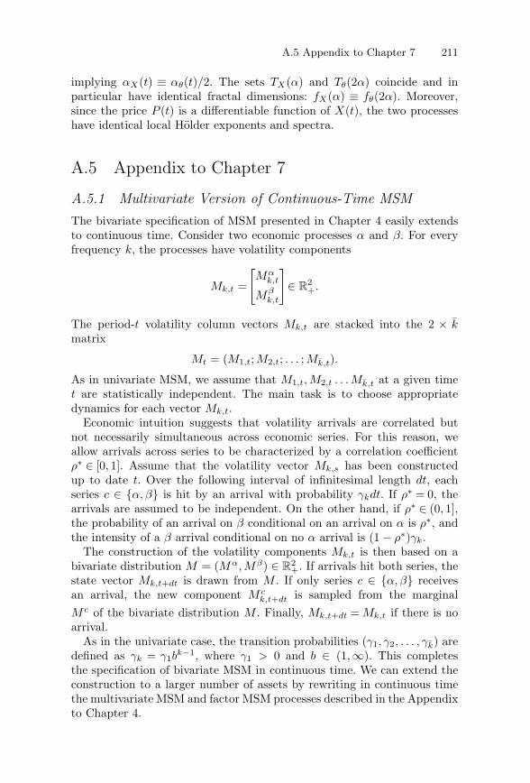
A.5 Appendix to Chapter 7 211

implying αX(t) ≡ αθ(t)/2. The sets TX(α) and Tθ(2α) coincide and inparticular have identical fractal dimensions: fX(α) ≡ fθ(2α). Moreover,since the price P (t) is a differentiable function of X(t), the two processeshave identical local Holder exponents and spectra.

A.5 Appendix to Chapter 7

A.5.1 Multivariate Version of Continuous-Time MSMThe bivariate specification of MSM presented in Chapter 4 easily extendsto continuous time. Consider two economic processes α and β. For everyfrequency k, the processes have volatility components

Mk,t =

[Mα

k,t

Mβk,t

]∈ R

2+.

The period-t volatility column vectors Mk,t are stacked into the 2 × kmatrix

Mt = (M1,t;M2,t; . . . ;Mk,t).

As in univariate MSM, we assume that M1,t, M2,t . . . Mk,t at a given timet are statistically independent. The main task is to choose appropriatedynamics for each vector Mk,t.

Economic intuition suggests that volatility arrivals are correlated butnot necessarily simultaneous across economic series. For this reason, weallow arrivals across series to be characterized by a correlation coefficientρ∗ ∈ [0, 1]. Assume that the volatility vector Mk,s has been constructedup to date t. Over the following interval of infinitesimal length dt, eachseries c ∈ {α, β} is hit by an arrival with probability γkdt. If ρ∗ = 0, thearrivals are assumed to be independent. On the other hand, if ρ∗ ∈ (0, 1],the probability of an arrival on β conditional on an arrival on α is ρ∗, andthe intensity of a β arrival conditional on no α arrival is (1 − ρ∗)γk.

The construction of the volatility components Mk,t is then based on abivariate distribution M = (Mα, Mβ) ∈ R

2+. If arrivals hit both series, the

state vector Mk,t+dt is drawn from M . If only series c ∈ {α, β} receivesan arrival, the new component M c

k,t+dt is sampled from the marginalM c of the bivariate distribution M . Finally, Mk,t+dt = Mk,t if there is noarrival.

As in the univariate case, the transition probabilities (γ1, γ2, . . . , γk) aredefined as γk = γ1b

k−1, where γ1 > 0 and b ∈ (1,∞). This completesthe specification of bivariate MSM in continuous time. We can extend theconstruction to a larger number of assets by rewriting in continuous timethe multivariate MSM and factor MSM processes described in the Appendixto Chapter 4.

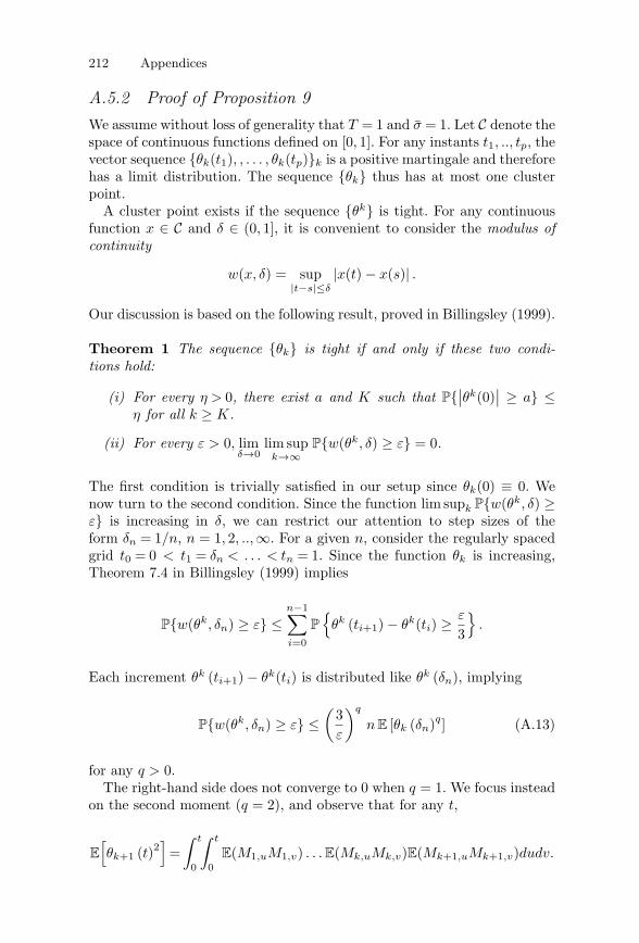
212 Appendices

A.5.2 Proof of Proposition 9We assume without loss of generality that T = 1 and σ = 1. Let C denote thespace of continuous functions defined on [0, 1]. For any instants t1, .., tp, thevector sequence {θk(t1), , . . . , θk(tp)}k is a positive martingale and thereforehas a limit distribution. The sequence {θk} thus has at most one clusterpoint.

A cluster point exists if the sequence {θk} is tight. For any continuousfunction x ∈ C and δ ∈ (0, 1], it is convenient to consider the modulus ofcontinuity

w(x, δ) = sup|t−s|≤δ

|x(t) − x(s)| .

Our discussion is based on the following result, proved in Billingsley (1999).

Theorem 1 The sequence {θk} is tight if and only if these two condi-tions hold:

(i) For every η > 0, there exist a and K such that P{∣∣θk(0)

∣∣ ≥ a} ≤η for all k ≥ K.

(ii) For every ε > 0, limδ→0

lim supk→∞

P{w(θk, δ) ≥ ε} = 0.

The first condition is trivially satisfied in our setup since θk(0) ≡ 0. Wenow turn to the second condition. Since the function lim supk P{w(θk, δ) ≥ε} is increasing in δ, we can restrict our attention to step sizes of theform δn = 1/n, n = 1, 2, ..,∞. For a given n, consider the regularly spacedgrid t0 = 0 < t1 = δn < . . . < tn = 1. Since the function θk is increasing,Theorem 7.4 in Billingsley (1999) implies

P{w(θk, δn) ≥ ε} ≤n−1∑

i=0

P

{θk (ti+1) − θk(ti) ≥ ε

3

}.

Each increment θk (ti+1) − θk(ti) is distributed like θk (δn), implying

P{w(θk, δn) ≥ ε} ≤(

3ε

)q

n E [θk (δn)q] (A.13)

for any q > 0.The right-hand side does not converge to 0 when q = 1. We focus instead

on the second moment (q = 2), and observe that for any t,

E

[θk+1 (t)2

]=∫ t

0

∫ t

0E(M1,uM1,v) . . . E(Mk,uMk,v)E(Mk+1,uMk+1,v)dudv.

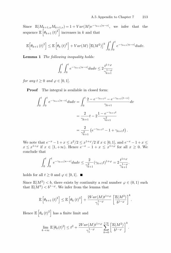
A.5 Appendix to Chapter 7 213

Since E(Mk+1,uMk+1,v) = 1 + V ar(M)e−γk+1|u−v|, we infer that the

sequence E

[θk+1 (t)2

]increases in k and that

E

[θk+1 (t)2

]≤ E

[θk (t)2

]+ V ar(M)

[E(M2)

]k∫ t

0

∫ t

0e−γk+1|u−v|dudv.

Lemma 1 The following inequality holds:

∫ t

0

∫ t

0e−γk+1|u−v|dudv ≤ 2

t1+ϕ

γ1−ϕk+1

for any t ≥ 0 and ϕ ∈ [0, 1].

Proof The integral is available in closed form:

∫ t

0

∫ t

0e−γk+1|u−v|dudv =

∫ t

0

2 − e−γk+1v − e−γk+1(t−v)

γk+1dv

=2

γk+1t − 2

1 − e−γk+1t

γ2k+1

=2

γ2k+1

(e−γk+1t − 1 + γk+1t

).

We note that e−x − 1 + x ≤ x2/2 ≤ x1+ϕ/2 if x ∈ [0, 1], and e−x − 1 + x ≤x ≤ x1+ϕ if x ∈ [1,+∞). Hence e−x − 1 + x ≤ x1+ϕ for all x ≥ 0. Weconclude that

∫ t

0

∫ t

0e−γk+1|u−v|dudv ≤ 2

γ2k+1

(γk+1t)1+ϕ = 2t1+ϕ

γ1−ϕk+1

.

holds for all t ≥ 0 and ϕ ∈ [0, 1]. ■

Since E(M2) < b, there exists by continuity a real number ϕ ∈ (0, 1) suchthat E(M2) < b1−ϕ. We infer from the lemma that

E

[θk+1 (t)2

]≤ E

[θk (t)2

]+

2V ar(M)t1+ϕ

γ1−ϕ1

[E(M2)b1−ϕ

]k

.

Hence E

[θk (t)2

]has a finite limit and

limk→∞

E [θk(t)2] ≤ t2 +2V ar(M)t1+ϕ

γ1−ϕ1

+∞∑

k=0

[E(M2)b1−ϕ

]k

.

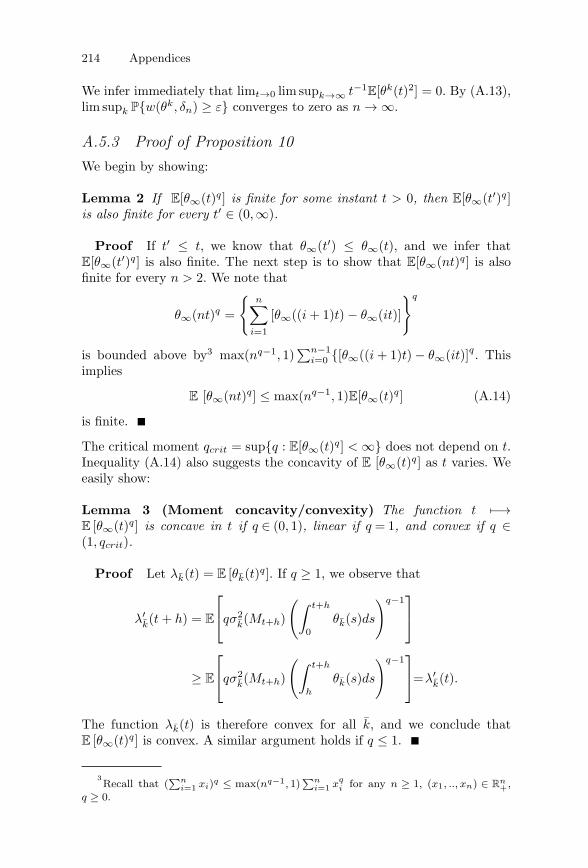
214 Appendices

We infer immediately that limt→0 lim supk→∞ t−1E[θk(t)2] = 0. By (A.13),

lim supk P{w(θk, δn) ≥ ε} converges to zero as n → ∞.

A.5.3 Proof of Proposition 10We begin by showing:

Lemma 2 If E[θ∞(t)q] is finite for some instant t > 0, then E[θ∞(t′)q]is also finite for every t′ ∈ (0,∞).

Proof If t′ ≤ t, we know that θ∞(t′) ≤ θ∞(t), and we infer thatE[θ∞(t′)q] is also finite. The next step is to show that E[θ∞(nt)q] is alsofinite for every n > 2. We note that

θ∞(nt)q =

{n∑

i=1

[θ∞((i + 1)t) − θ∞(it)]

}q

is bounded above by3 max(nq−1, 1)∑n−1

i=0 {[θ∞((i + 1)t) − θ∞(it)]q. Thisimplies

E [θ∞(nt)q] ≤ max(nq−1, 1)E[θ∞(t)q] (A.14)

is finite. ■

The critical moment qcrit = sup{q : E[θ∞(t)q] < ∞} does not depend on t.Inequality (A.14) also suggests the concavity of E [θ∞(t)q] as t varies. Weeasily show:

Lemma 3 (Moment concavity/convexity) The function t �−→E [θ∞(t)q] is concave in t if q ∈ (0, 1), linear if q = 1, and convex if q ∈(1, qcrit).

Proof Let λk(t) = E [θk(t)q]. If q ≥ 1, we observe that

λ′k(t + h) = E

⎡

⎣qσ2k(Mt+h)

(∫ t+h

0θk(s)ds

)q−1⎤

⎦

≥ E

⎡

⎣qσ2k(Mt+h)

(∫ t+h

h

θk(s)ds

)q−1⎤

⎦=λ′k(t).

The function λk(t) is therefore convex for all k, and we conclude thatE [θ∞(t)q] is convex. A similar argument holds if q ≤ 1. ■

3Recall that (

∑ni=1 xi)q ≤ max(nq−1, 1)

∑ni=1 xq

i for any n ≥ 1, (x1, .., xn) ∈ Rn+,

q ≥ 0.

A.5 Appendix to Chapter 7 215

For any k ∈ {1, . . .∞}, let Θk(γ1) denote the trading time θk(1) at t = 1in continuous-time MSM with frequency parameters γ1 and b.

Lemma 4 (Invariance property) Trading time satisfies

θ∞(t) d= tΘ∞(tγ1) (A.15)

for all t ∈ [0,∞) and γ1 > 0.

Proof For any finite k, trading time is given by θk(t) ≡∫ t

0 σ2k(Ms)ds.

Consider the change of variables u = s/t. We infer that

θk(t) ≡ t

∫ 1

0σ2

k(Mut)du.

The state vector M ′u = Mut is driven by arrivals of intensity tγ1, . . . ,

tγ1bk−1. We conclude that θk(t) d= tΘk(tγ1) for all k, implying θ∞(t) d=

tΘ∞(tγ1). ■

When the frequency γ is close to zero, the first-stage multiplier is constanton the unit interval with high probability, which suggests that Θ∞(γ) ≈M Θ∞(bγ) and thus E[Θ∞(γ)q] ≈ E(Mq) E[Θ∞(bγ)q]. This intuition canbe used to show:

Lemma 5 (Scaling) E [Θ∞(γ)q] ∼ E(Mq) E [Θ∞(bγ)q] as γ → 0.

Proof We consider g(γ) = E [Θ∞(γ)q]. Let t1 < . . . < tN denote thedates in the unit interval when a first-stage multiplier is drawn. We alsodefine t0 = 0 and tN+1 = 1. Simple conditioning implies

g(γ) = E(Mq) g(bγ) e−γ +∞∑

n=1

e−γγn

n!E [Θ∞(γ)q|N = n] .

As in the proof of lemma 2, the relation Θ∞(γ) =∑N

j=0 [θ∞(tj+1) − θ∞(tj)]implies

Θ∞(γ)q ≤ max[(N + 1)q−1, 1

] N∑

j=0

[θ∞(tj+1) − θ∞(tj)]q.

The conditional expectation E [Θ∞(γ)q|N = n] is therefore boundedabove by

max[(n + 1)q−1, 1

](n + 1)E(Mq)g(bγ).

216 Appendices

and thus

1 ≤ eγg(γ)E(Mq) g(bγ)

≤ 1 +∞∑

n=1

γn

n!(n + 1)max(q,1).

This implies g(γ) ∼ E(Mq) g(bγ) when γ → 0. ■

The qth moment of trading time satisfies E {[θ∞(t)]q} ∼ [E(Mq)/bq]E {[θ∞(bt)]q}. Combined with Lemma 3, this property implies thatE {[θ∞(t)]q} ∼ cqt

τθ(q)+1as t → 0. We also infer from Lemma 3 that

τθ(q) > 0 for all admissible moments greater than unity, implying thatτθ(qcrit) ≥ 0.

A.5.4 Proof of Corollary 1We know that the restriction of (θk) on any bounded subinterval [0, T ] isuniformly equicontinuous and has a continuous limiting process. Theorem16.8 in Billingsley (1999) implies that the sequence θk is also tight onD[0,∞). We conclude that the sequence θk converges in D[0,∞) to a limitprocess θ∞ with continuous sample paths.

A.5.5 Proof of Proposition 11Our proof is based on the following result, proved in Billingsley (1999).

Theorem 2 If

[θ∗k(t1), .., θ∗

k(tp)]d→ [θ(t1), .., θ(tp)] (A.16)

holds for all t1, .., tp, and if

limδ→0

lim supk→∞

P{w(θ∗k, δ) ≥ ε} = 0 (A.17)

for each positive ε, then θ∗k weakly converges to θ.

We successively establish the convergence of the marginals (A.16) and thetightness condition (A.17).

Convergence of the Marginals

The proof is based on coupled trading times. We assume without loss ofgenerality that T = 1 and σ = 1. Consider the sequence {θk}∞

k=1 used inthe construction of the continuous time trading time θ∞, and assume forsimplicity that {θk}∞

k=1 is defined on [0,∞). Stage k relies on the startingtime tk,0 = 0, and arrival times tk,n (n ≥ 1). The difference between twoconsecutive arrivals, Ek,n+1 = tk,n+1−tk,n, has an exponential distributionwith density γk exp(−γkt). By a slight abuse of notation, we denote by Mk,n

the value of the multiplier over the interval [tk,n; tk,n+1).

A.5 Appendix to Chapter 7 217

We can similarly construct a coupled trading time θ∗k

with discretizedarrival times. Let [x] denote for all x ∈ R the unique integer such that[x] ≤ x < [x] + 1. For a given integer c > 1, consider the uniform grid 0,1/ck, .., 1. We discretize the sequence {tk,n} on the grid by lettingsk,0 = 0, and

sk,n =n∑

i=1

[ckEk,i] + 1ck

for every n ≥ 1.

We observe that the random variable ck(sk,n+1 − sk,n) has a geometricdistribution with parameter γk,k = 1 − exp(−γ1b

k−1/ck) since

P

{sk,n+1 − sk,n =

m

ck

}= P

{m − 1

ck≤ Ek,n+1 <

m

ck

}= (1−γk,k)m−1γk,k.

The multiplier over [sk,n, sk,n+1) is set equal to the value Mk,n of themultiplier on the fixed interval [tk,n; tk,n+1) in the continuous construction.

Let N∗k denote the highest integer n such that sk,n < 1 in the kth stage

of the discrete-time construction. For any n1, .., nk, let Δ∗(n1, .., nk) be thelength of the largest subinterval of [0, 1] over which multipliers are givenby M1,n1 , . . . , Mk,nk

.4 We know that

θ∗k(1) =

N∗1∑

n1=0

. . .

N∗k∑

nk=0

M1,n1 . . . Mk,nkΔ∗(n1, .., nk).

For the continuous-time construction, we can similarly define Nk andΔ(n1, .., nk), and write

θk(1) =N1∑

n1=0

. . .

Nk∑

nk=0

M1,n1 . . . Mk,nkΔ(n1, .., nk).

Let Hk = max(N∗k , Nk). The intervals attached to a given set of multipliers

in the paired constructions differ in length by:

δn1,..,nk= Δ∗(n1, .., nk) − Δ(n1, .., nk).

With this notation, the discretized and continuous versions of trading timediffer by

θ∗k(1) − θk(1) =

H1∑

n1=0

. . .

Hk∑

nk=0

M1,n1 . . . Mk,nkδn1,..,nk

. (A.18)

4That is, Δ∗(n1, .., nk) is the length of the intersection of [sk,nk

; min(1, sk,nk+1)),k ∈ {1, .., k}.

218 Appendices

As is shown below, the first or second moment of∣∣θ∗

k(1) − θk(1)

∣∣ convergesto zero as k → ∞. Since this argument applies equally well to all timeintervals, we conclude that θ∗

k(t) d→ θ∞(t) for all t.

First Moment. We note that

E∣∣θ∗

k(1) − θk(1)∣∣ ≤ E

⎛

⎝∑

n1,...,nk

∣∣δn1,..,nk

∣∣

⎞

⎠.

The average number of nonzero mismatches δn1,..,nkin the unit interval

is of order bk, and their size is of order 1/ck. As in Calvet and Fisher(2001), we can therefore verify that the first moment E

∣∣θ∗k(1) − θk(1)

∣∣ isbounded above by a multiple of (b/c)k. Hence E

∣∣θ∗k(1) − θk(1)

∣∣ → 0 underCondition 5.

Second Moment. We note that

E

{[θ∗

k(1) − θk(1)]2} ≤

[E(M2)

]kE

⎛

⎝∑

m1,...,mk,n1,...,nk

δm1,..,mkδn1,..,nk

⎞

⎠.

(A.19)

The number of nonzero δm1,..,mkδn1,..,nk

is of order bk, while their size is of

order c−2k. We can verify that the second moment E

{[θ∗

k(1) − θk(1)

]2} is

bounded above by a multiple of[E(M2)b/c2

]k and therefore converges tozero under Condition 6.

Tightness

Let δ = c−l. As in the proof of Proposition 9, we infer from Theorem 7.4in Billingsley (1999) that for any k ≥ 1,

P{w(θ∗k, δ) ≥ ε} ≤ δ−1

P{θ∗

k(δ) ≥ ε/3}

.

Since θ∗k(δ) d→ θ∞(δ), the function lim supk P{w(θ∗

k, δ) ≥ ε} is bounded

above by δ−1P {θ∞ (δ) ≥ ε/3}. Given a number q > 0 satisfying τθ(q) > 0,

Chebyshev’s inequality implies that lim supk P{w(θ∗k, δ) ≥ ε} is bounded

above by (3/ε)q δ−1E [θ∞ (δ)q]. Letting δ → 0, we infer that δ−1

E [θ∞ (δ)q] ∼cqδ

τθ(q) → 0 and conclude that condition (A.17) is satisfied. We have thusestablished that θ∗

kweakly converges to θ∞ as k → ∞.

A.5.6 MSM with Dependent ArrivalsTo aid the discussion, let At denote the set of arrival instants forcomponent k. In Calvet and Fisher (1999, 2001), we specify that if anarrival occurs in component k at instant t, then arrivals are triggered inall higher-frequency components k′ > k. Hence Ak ⊆ Ak′ for all k′ > k.In addition, we assume that arrivals that are specific to stage-k can occur

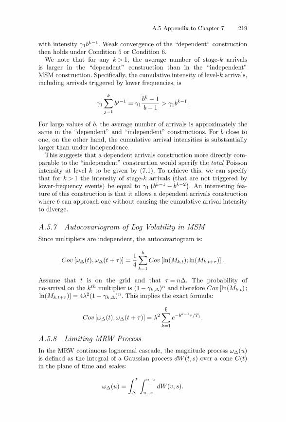
A.5 Appendix to Chapter 7 219

with intensity γ1bk−1. Weak convergence of the “dependent” construction

then holds under Condition 5 or Condition 6.We note that for any k > 1, the average number of stage-k arrivals

is larger in the “dependent” construction than in the “independent”MSM construction. Specifically, the cumulative intensity of level-k arrivals,including arrivals triggered by lower frequencies, is

γ1

k∑

j=1

bj−1 = γ1bk − 1b − 1

> γ1bk−1.

For large values of b, the average number of arrivals is approximately thesame in the “dependent” and “independent” constructions. For b close toone, on the other hand, the cumulative arrival intensities is substantiallylarger than under independence.

This suggests that a dependent arrivals construction more directly com-parable to the “independent” construction would specify the total Poissonintensity at level k to be given by (7.1). To achieve this, we can specifythat for k > 1 the intensity of stage-k arrivals (that are not triggered bylower-frequency events) be equal to γ1

(bk−1 − bk−2

). An interesting fea-

ture of this construction is that it allows a dependent arrivals constructionwhere b can approach one without causing the cumulative arrival intensityto diverge.

A.5.7 Autocovariogram of Log Volatility in MSMSince multipliers are independent, the autocovariogram is:

Cov [ωΔ(t), ωΔ(t + τ)] =14

k∑

k=1

Cov [ln(Mk,t); ln(Mk,t+τ )] .

Assume that t is on the grid and that τ = nΔ. The probability ofno-arrival on the kth multiplier is (1 − γk,Δ)n and therefore Cov [ln(Mk,t) ;ln(Mk,t+τ )] = 4λ2(1 − γk,Δ)n. This implies the exact formula:

Cov [ωΔ(t), ωΔ(t + τ)] = λ2k∑

k=1

e−bk−1τ/T1 .

A.5.8 Limiting MRW ProcessIn the MRW continuous lognormal cascade, the magnitude process ωΔ(u)is defined as the integral of a Gaussian process dW (t, s) over a cone C(t)in the plane of time and scales:

ωΔ(u) =∫ T

Δ

∫ u+s

u−s

dW (v, s).

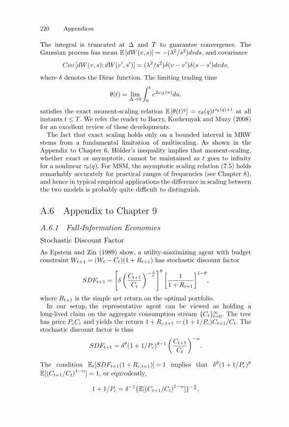
220 Appendices

The integral is truncated at Δ and T to guarantee convergence. TheGaussian process has mean E [dW (v, s)] = −(λ2/s2)dvds, and covariance

Cov [dW (v, s); dW (v′, s′)] = (λ2/s2)δ(v − v′)δ(s − s′)dvds,

where δ denotes the Dirac function. The limiting trading time

θ(t) = limΔ→0

∫ t

0e2ωΔ(u)du.

satisfies the exact moment-scaling relation E [θ(t)q] = cθ(q)tτθ(q)+1 at allinstants t ≤ T . We refer the reader to Bacry, Kozhemyak and Muzy (2008)for an excellent review of these developments.

The fact that exact scaling holds only on a bounded interval in MRWstems from a fundamental limitation of multiscaling. As shown in theAppendix to Chapter 6, Holder’s inequality implies that moment-scaling,whether exact or asymptotic, cannot be maintained as t goes to infinityfor a nonlinear τθ(q). For MSM, the asymptotic scaling relation (7.5) holdsremarkably accurately for practical ranges of frequencies (see Chapter 8),and hence in typical empirical applications the difference in scaling betweenthe two models is probably quite difficult to distinguish.

A.6 Appendix to Chapter 9

A.6.1 Full-Information Economies

Stochastic Discount Factor

As Epstein and Zin (1989) show, a utility-maximizing agent with budgetconstraint Wt+1 = (Wt − Ct)(1 + Rt+1) has stochastic discount factor

SDFt+1 =

[δ

(Ct+1

Ct

)− 1ψ

]θ [1

1 + Rt+1

]1−θ

,

where Rt+1 is the simple net return on the optimal portfolio.In our setup, the representative agent can be viewed as holding a

long-lived claim on the aggregate consumption stream {Ct}∞t=0. The tree

has price PcCt and yields the return 1 + Rc,t+1 = (1 + 1/Pc)Ct+1/Ct. Thestochastic discount factor is thus

SDFt+1 = δθ(1 + 1/Pc)θ−1(

Ct+1

Ct

)−α

.

The condition Et[SDFt+1(1 + Rc,t+1)] = 1 implies that δθ(1 + 1/Pc)θ

E[(Ct+1/Ct)1−α] = 1, or equivalently,

1 + 1/Pc = δ−1{E[(Ct+1/Ct)1−α]}− 1

θ .

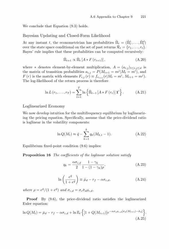
A.6 Appendix to Chapter 9 221

We conclude that Equation (9.3) holds.

Bayesian Updating and Closed-Form Likelihood

At any instant t, the econometrician has probabilities Πt = (Π1t , . . . , Π

dt )

over the state space conditional on the set of past returns Rt = {r1, . . . , rt}.Bayes’ rule implies that these probabilities can be computed recursively:

Πt+1 ∝ Πt [A ∗ F (rt+1)] , (A.20)

where ∗ denotes element-by-element multiplication, A = (ai,j)1≤i,j≤d isthe matrix of transition probabilities ai,j = P (Mt+1 = mj |Mt = mi), andF (r) is the matrix with elements Fi,j (r) ≡ frt+1(r|Mt = mi, Mt+1 = mj).The log-likelihood of the return process is therefore

lnL (r1, . . . , rT ) =T∑

t=1

ln{

Πt−1 [A ∗ F (rt)]1′}

. (A.21)

Loglinearized Economy

We now develop intuition for the multifrequency equilibrium by loglineariz-ing the pricing equation. Specifically, assume that the price-dividend ratiois loglinear in the volatility components:

lnQ(Mt) ≈ q −k∑

k=1

qk(Mk,t − 1). (A.22)

Equilibrium fixed-point condition (9.6) implies:

Proposition 16 The coefficients of the loglinear solution satisfy

qk =ασc,d

21 − γk

1 − (1 − γk)ρ, (A.23)

ln(

eq

1 + eq

)≡ μd − rf − ασc,d, (A.24)

where ρ = eq/(1 + eq) and σc,d = σcσdρc,d.

Proof By (9.6), the price-dividend ratio satisfies the loglinearizedEuler equation:

lnQ(Mt) = μd − rf − ασc,d + ln Et

{[1 + Q(Mt+1)]e−ασcρc,d[σd(Mt+1)−σd]

}.

(A.25)

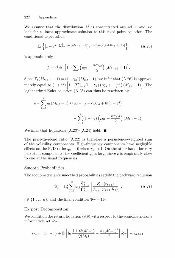
222 Appendices

We assume that the distribution M is concentrated around 1, and welook for a linear approximate solution to this fixed-point equation. Theconditional expectation

Et

{[1 + eq−

∑kk=1 qk(Mk,t+1−1)]e−ασcρc,d[σd(Mt+1)−σd]

}(A.26)

is approximately

(1 + eq)Et

[1 −

∑(ρqk +

ασc,d

2

)(Mk,t+1 − 1)

].

Since Et(Mk,t+1 − 1) = (1 − γk)(Mk,t − 1), we infer that (A.26) is approxi-

mately equal to (1 + eq)[1 −

∑kk=1(1 − γk)

(ρqk + ασc,d

2

)(Mk,t − 1)

]. The

loglinearized Euler equation (A.25) can thus be rewritten as:

q −k∑

k=1

qk(Mk,t − 1) ≈ μd − rf − ασc,d + ln(1 + eq)

−k∑

k=1

(1 − γk)(ρqk +

ασc,d

2

)(Mk,t − 1).

We infer that Equations (A.23)–(A.24) hold. ■

The price-dividend ratio (A.22) is therefore a persistence-weighted sumof the volatility components. High-frequency components have negligibleeffects on the P/D ratio: qk → 0 when γk → 1. On the other hand, for verypersistent components, the coefficient qk is large since ρ is empirically closeto one at the usual frequencies.

Smooth Probabilities

The econometrician’s smoothed probabilities satisfy the backward recursion

Ψit = Πi

t

d∑

j=1

aij

Ψjt+1

Πjt+1

[Fi,j (rt+1)

frt+1 (rt+1|Rt)

], (A.27)

i ∈ {1, . . . , d}, and the final condition ΨT = ΠT .

Ex post Decomposition

We condition the return Equation (9.9) with respect to the econometrician’sinformation set RT :

rt+1 = μd − rf + E

[ln

1 + Q(Mt+1)Q(Mt)

− σd(Mt+1)2

2

∣∣∣∣RT

]+ ed,t+1.

A.6 Appendix to Chapter 9 223

The definition of smoothed probabilities implies

rt+1 = μd − rf + EΨt+1

(ln[1 + Q(Mt+1)] − σd(Mt+1)2/2

)

− EΨtlnQ(Mt) + ed,t+1.

Since EΨtrt+1 = μd −rf +EΨt

(ln[1+Q(Mt+1)]−σd(Mt+1)2/2− lnQ(Mt)),we conclude that (9.11) holds.

The Campbell-Hentschel Model

The CH specification is based on a QGARCH(1, 2) process for dividendnews (Engle, 1990; Sentana, 1995). Excess returns satisfy

rt+1 = μ + γσ2t + (1 + 2λb)ηd,t+1 − λ

(η2

d,t+1 − σ2t

), (A.28)

where the dividend news ηd,t+1 is N(0, σ2

t

), with

σ2t = � + α1 (ηd,t − b)2 + α2 (ηd,t−1 − b)2 + βσ2

t−1,

λ =γρ (α1 + ρα2)

1 − ρ (α1 + ρα2 + β).

The parameter ρ is calibrated to the empirical price-dividend ratio, and thesevenparameters (μ, γ, �, α1, α2, b, β) are estimatedbymaximum likelihood.

The conditional return Etrt+1 = μ+γσ2t increases in conditional volatil-

ity and γ, which is related to risk aversion. Feedback appears in (A.28)through a quadratic term in dividend news, λ(2bηd,t+1 + σ2

t − η2d,t+1).

After an extreme innovation ηd,t+1, the investor knows that volatility willincrease, and price drops. The location parameter b differentiates QGARCHfrom traditional GARCH. When b > 0, negative dividend news ηd,t has ahigher impact on volatility than positive news of the same size.

A.6.2 Learning EconomiesConsider the volatility state and investor probability distribution (Mt,Πt)at the end of period t. The state of the economy in the following period iscomputed in three steps.

First, we compute the latent state of nature at date t+1. That is, we drawthe volatility state Mt+1 given Mt, and sample k +2 independent standardnormals (z1,t+1; . . . ; zk,t+1; εd,t+1; ηc,t+1). The Gaussian consumption noise

is εc,t+1 = ρc,dεd,t+1+√

1 − ρ2c,dηc,t+1. We then compute the consumption,

dividend, and signal in period t + 1.Second, we compute the corresponding investor belief. The investor

observes (δt+1, ct+1 − ct, dt+1 − dt) and uses Bayes’ rule to derive her

224 Appendices

new probability distribution over volatility states: Πjt+1 ∝ f(δt+1, ct+1 −

ct, dt+1 − dt|Mt+1 = mj)∑d

i=1 ai,jΠit.

Third, we compute the corresponding excess return using (9.16).

A.6.3 Multifrequency Consumption RiskIn the presence of consumption switches, the tree has price Pc(M ′

t)Ct, andthe stochastic discount factor is given by

SDFt+1 = δθ

[1 + Pc(M ′

t+1)Pc(M ′

t)

]θ−1(Ct+1

Ct

)−α

.

We index the consumption states by i = 1, . . . , N = 2. Let πi,j denote thetransition probability from state i to state j. The price-consumption ratiosatisfies the fixed-point equation

Pc(i) = δ

⎛

⎝N∑

j=1

πi,j [1 + Pc(j)]θe(1−α)gc(j)+σ2

c(j)(1−α)2/2

⎞

⎠1/θ

. (A.29)

The interest rate rf = − ln Et(SDFt+1) is then

rf (i) = −θ ln δ − ln

⎧⎨

⎩∑

j

πi,j

[1 + Pc(j)

Pc(i)

]θ−1

e−αgc(j)+α2σ2c(j)/2

⎫⎬

⎭ .

Finally, the price-dividend ratio of the stock satisfies the fixed-pointequation

Q(Mt) = δθEt

{[1 + Pc(M ′

t+1)Pc(M ′

t)

]θ−1

eφ(Mt+1,M ′t+1)[1 + Q(Mt+1)]

},

(A.30)

where φ(Mt+1, M ′t+1) = μd(Mt+1) − αgc(M ′

t+1) + α2σ2c (M ′

t+1) / 2 − ασc

(M ′t+1)σd(Mt+1)ρc,d.

A.7 Appendix to Chapter 10

A.7.1 Proof of Proposition 13The price-dividend ratio satisfies

Q(Mt) = E

(∫ +∞

0

Λt+s

Λt

Dt+s

Dtds

∣∣∣∣Mt

).

A.7 Appendix to Chapter 10 225

Since

d ln Λt =[−rf (Mt) − α2σ2

C(Mt)/2]dt − ασC(Mt)dZC(t),

d lnDt =[gD(Mt) − σ2

D(Mt)/2]dt + σD(Mt)dZD(t),

we infer that

lnΛt+s

Λt+ ln

Dt+s

Dt=∫ s

0

[gD(Mt+h) − rf (Mt+h)

− σ2D(Mt+h) + α2σ2

C(Mt+h)2

]dh

+∫ s

0[σD(Mt+h)dZD(t + h) − ασC(Mt+h)dZC(t + h)]

is conditionally Gaussian with mean∫ s

0

[gD(Mt+h) − rf (Mt+h) −

σ2D(Mt+h)+α2σ2

C(Mt+h)2

]dh and variance

∫ s

0 [α2σ2C(Mt+h) + σ2

D(Mt+h) −2αρC,DσC(Mt+h)σD(Mt+h)]dh. We then easily check that

E

(Λt+s

Λt

Dt+s

Dt

∣∣∣∣Mt

)= Ete

∫ s0 [gD(Mt+h)−rf (Mt+h)−αρC,DσC(Mt+h)σD(Mt+h)]dh.

A.7.2 Multivariate ExtensionsThe asset pricing models in the main text are based on univariate MSMand assume either i.i.d. consumption or Lucas tree economies. We nowintroduce an extension of MSM that permits intermediate comovements ofconsumption and dividends. As in multivariate MSM (see Chapter 4 andAppendix to Chapter 7), we assume that the consumption and dividendprocesses have constant drifts but stochastic volatilities

σC(Mt) = σC(Mα1,tM

α2,t . . . Mα

,t)1/2,

σD(Mt) = σD(Mβ1,tM

β2,t . . . Mβ

k,t)1/2,

where � ≤ k. The specification permits correlation in volatility across seriesthrough the bivariate distribution M and correlation in returns through theBrownian motions ZC and ZD. This flexible setup permits us to constructa more general class of jump-diffusions for stock prices. We note that themodel reduces to i.i.d. consumption if � = 0, and to a Lucas tree economyif � = k and multipliers are perfectly correlated.

226 Appendices

The generalized model might also be useful for option pricing. In ourenvironment, the price of a European option f(PT ) is therefore given by5

f0 = E0

[ΛT

Λ0f(PT )

].

As in Hull and White (1987), let f [(Mt)t∈[0,T ]] = E0 [ΛT f(PT )/Λ0|(Mt)t∈[0,T ]

]denote the option price conditional on the state history. The

law of iterated expectations implies f0 = E0f((Mt)t∈[0,T ]

), which can be

useful in empirical settings.

A.7.3 Proof of Proposition 14Given an initial state νt, the P/D ratio of the Lucas tree economy can bewritten as

Q(ε) = E

(∫ +∞

0e−δ′s− α(1−α)

2

∫ s0 (σ2

D[Mt+h(ε)]−σ2D)dhds

∣∣∣∣ νt

).

We note that Q(0) = 1/δ′. By the dominated convergence theorem, thefunction Q is differentiable and

Q′(0) = −q1E

⎧⎨

⎩

∫ +∞

0e−δ′s

⎡

⎣∫ s

0

k∑

k=1

(νk,t+h − 1)dh

⎤

⎦ ds

∣∣∣∣∣∣νt

⎫⎬

⎭.

Since Et(νk,t+h − 1) = e−γkh(νk,t − 1), we infer that

Q′(0) = −q1

k∑

k=1

(νk,t − 1)(∫ +∞

0e−δ′s

∫ s

0e−γkhdh ds

)

= −q1

k∑

k=1

νk,t − 1δ′(δ′ + γk)

.

Hence

Q(ε) = Q(0)

⎛

⎝1 − q1

k∑

k=1

νk,t − 1δ′ + γk

ε

⎞

⎠+ o(ε).

We take the log and conclude that (10.7) holds. A similar argument holdsin the i.i.d. consumption case.

5See Anderson and Raimondo (2005), David and Veronesi (2002), Garcia, Luger,

and Renault (2003) and Garleanu, Pedersen, and Poteshman (2006) for recent work onconsumption-based option pricing.

A.7 Appendix to Chapter 10 227

A.7.4 Proof of Proposition 15Consider

Qk(t) ≡ E

[∫ +∞

0e−ρse−λ[θk(t+s)−θk(t)]ds

∣∣∣∣Mt

],

where λ = α(1 − α)/2 > 0. We easily check that Qk(t) is a positive andbounded submartingale:

Qk(t) ≤ Ek

[Qk+1(t)

]≤ 1/ρ.

The P/D ratio Qk(t) therefore converges to a limit distribution, which wenow easily characterize.

Consider the function Φ : D[0,∞) → D[0,∞) defined for every cadlagfunction f by the integral transform

(Φf)(t) =∫ +∞

0exp {−ρs − λ[f(t + s) − f(t)]} ds.

The function Φ is bounded with respect to the Skorohod distance since(Φf)(t) ∈ [0, 1/ρ] for all t. We also check that it is continuous. Since θk →θ∞, we infer that Φθk weakly converges to Φθ∞. Hence, Qk(t) → Q∞(t),and the proposition holds.

References

Abadir, K. M., W. Distaso, and L. Giraitis. 2008. Two estimators of the long-runvariance: beyond short memory. Working paper. Imperial College London.

Abel, A. 1988. Stock prices under time-varying dividend risk: an exact solution inan infinite horizon general equilibrium model. Journal of Monetary Economics22: 375–95.

Abel, A. 1999. Risk premia and term premia in general equilibrium. Journal ofMonetary Economics 43: 3–33.

Abel, A. 2003. The effects of a baby boom on stock prices and capital accumulationin the presence of social security. Econometrica 71: 551–78.

Adelman, I. 1965. Long cycles: fact or artefact? American Economic Review 55:444–63.

Adrian, T. and J. Rosenberg. 2008. Stock returns and volatility: pricing the long-runand short-run components of market risk. Journal of Finance, forthcoming.

Agterberg, F. 2007. New applications of the model of de Wijs in regional geo-chemistry. Mathematical Geology 39: 1–25.

Ait-Sahalia, Y. 2002. Telling from discrete data whether the underlying continuous-time model is a diffusion. Journal of Finance 57: 2075–112.

Ait-Sahalia, Y. and J. Jacod. 2008. Testing for jumps in a discretely observedprocess. Annals of Statistics, forthcoming.

Akgiray, V. 1989. Conditional heteroskedasticity in time series of stock returns:evidence and forecasts. Journal of Business 62: 55–80.

Albert, J. and S. Chib. 1993. Bayes inference via Gibbs sampling of autoregressivetime series subject to Markov means and variance shifts. Journal of Business andEconomic Statistics 11: 1–15.

Alizadeh, S., M. Brandt, and F. X. Diebold. 2002. Range-based estimation ofstochastic volatility models. Journal of Finance 57: 1047–91.

Andersen, T. 1994. Stochastic autoregressive volatility: a framework for volatilitymodeling. Mathematical Finance 4: 75–102.

Andersen, T. 1996. Return volatility and trading volume: an information flow inter-pretation of stochastic volatility. Journal of Finance 51: 169–204.

Andersen, T. G. and L. Benzoni. 2008. Stochastic volatility. In Encyclopedia ofComplexity and System Science, ed. B. Mizrach. Springer.

Andersen, T., L. Benzoni, and J. Lund. 2002. An empirical investigation ofcontinuous-time models for equity returns. Journal of Finance 57: 1239–84.

Andersen, T. and T. Bollerslev. 1998a. Answering the skeptics: yes, standard vola-tility models do provide accurate forecasts. International Economic Review 39:885–905.

Andersen, T. and T. Bollerslev. 1998b. Deutsche-mark dollar volatility: intradayactivity patterns, macroeconomic announcements, and longer-run dependencies.Journal of Finance 53: 219–65.

Andersen, T., T. Bollerslev, and F. X. Diebold. 2007. Roughing it up: including jumpcomponents in the measurement, modeling, and forecasting of return volatility.Review of Economics and Statistics 89: 701–20.

230 References

Andersen, T., T. Bollerslev, F. X. Diebold, and P. Labys. 2001. The distribution ofrealized exchange rate volatility. Journal of the American Statistical Association96: 42–55.

Andersen, T., T. Bollerslev, F. X. Diebold, and P. Labys. 2003. Modeling andforecasting realized volatility. Econometrica 71: 579–625.

Andersen, T., T. Bollerslev, F. X. Diebold, and C. Vega. 2003. Real-time pricediscovery in foreign exchange. American Economic Review 93: 38–62.

Andersen, T., T. Bollerslev, and N. Meddahi. 2005. Correcting the errors: volatilityforecast evaluation using high-frequency data and realized volatilities. Econo-metrica 73: 279–96.

Andersen, T. and B. Sørensen. 1996. GMM estimation of a stochastic volatility model:a Monte Carlo study. Journal of Business and Economic Statistics 14: 328–52.

Anderson, R. M. and R. C. Raimondo. 2005. Market clearing and derivative pricing.Economic Theory 25: 21–34.

Andrews, D. F. and C. L. Mallows. 1974. Scale mixtures of normal distributions.Journal of the Royal Statistical Society B 36: 99–102.

Andrews, D. W. K. 1991. Heteroskedasticity and autocorrelation consistent covari-ance matrix estimation. Econometrica 59: 817–54.

Andrews, D. W. K. and P. Guggenberger. 2003. A bias-reduced log-periodogramregression for the long-memory parameter. Econometrica 71: 675–712.

Andrews, D. W. K. and C. Monahan. 1992. An improved heteroskedasticity andautocorrelation consistent covariance matrix estimator. Econometrica 60: 953–66.

Arneodo, A., J.-P. Bouchaud, R. Cont, J.-F. Muzy, M. Potters, and D. Sornette.1996. Comment on “Turbulent cascades in foreign exchange markets,” arXiv:cond-mat/9607120v1.

Arneodo, A., J.-F. Muzy, and D. Sornette. 1998. Direct causal cascade in the stockmarket. European Physical Journal B 2: 277–82.

Arthur, W. B., J. Holland, B. LeBaron, R. Palmer, and P. Tayler. 1997. Asset pricingunder endogenous expectations in an artificial stock market. In The Economy asan Evolving Complex System II, eds. W. B. Arthur, S. N. Durlauf, and D. Lane,pp. 15–44. Addison-Wesley.

Attanasio, O. and G. Weber. 1993. Consumption growth, the interest rate, andaggregation. Review of Economic Studies 60: 631–49.

Atzori, L., N. Aste, and M. Isola. 2006. Estimation of multifractal parameters intraffic measurement: an accuracy-based real-time approach. Computer Communi-cations 29: 1879–88.

Aydemir, A. C., M. Gallmeyer, and B. Hollifield. 2006. Financial leverage does notcause the leverage effect. Working paper. Texas A&M University and CarnegieMellon University.

Bachelier, L. 1900. Theory of speculation. In The Random Character of Stock MarketPrices, ed. P. Cootner. MIT Press, 1964, Reprint.

Backus, D. K. and S. E. Zin. 1993. Long memory inflation uncertainty: evidencefrom the term structure of interest rates. Journal of Money, Credit and Banking25: 681–700.

Bacry, E., J. Delour, and J.-F. Muzy. 2001. Multifractal random walks. PhysicalReview E 64: 026103–06.

Bacry, E., A. Kozhemyak, and J.-F. Muzy. 2008. Continuous cascade models forasset returns. Journal of Economic Dynamics and Control 32(1): 156–99.

Bacry, E. and J.-F. Muzy. 2003. Log-infinitely divisible multifractal processes.Communications in Mathematical Physics 236: 449–75.

Baillie, R. 1996. Long memory processes and fractional integration in econometrics.Journal of Econometrics 73: 5–59.

Baillie, R. and T. Bollerslev. 1989. The message in daily exchange rates: a conditionalvariance tale. Journal of Business and Economic Statistics 7: 297–305.

References 231

Baillie, R., T. Bollerslev, and H. O. Mikkelsen. 1996. Fractionally integrated gener-alized autoregressive conditional heteroscedasticity. Journal of Econometrics 74:3–30.

Baillie, R., C. F. Chung, and M. A. Tieslau. 1996. Analyzing inflation by the frac-tionally integrated ARFIMA-GARCH model. Journal of Applied Econometrics11: 23–40.

Bakshi, G., H. Cao, and X. Chen. 1997. Empirical performance of alternative optionpricing models. Journal of Finance 52: 2003–49.

Ball, C. and W. Torous. 1985. On jumps in common stock prices and their impacton call option pricing. Journal of Finance 40: 155–73.

Bansal, R., V. Khatchatrian, and A. Yaron. 2005. Interpretable asset markets?European Economic Review 49: 531–60.

Bansal, R. and C. Lundblad. 2002. Market efficiency, fundamental values, and thesize of the risk premium in global equity markets. Journal of Econometrics 109:195–237.

Bansal, R. and A. Yaron. 2004. Risks for the long run: a potential resolution of assetpricing puzzles. Journal of Finance 49: 1481–509.

Bansal, R. and H. Zhou. 2002. Term structure of interest rates with regime shifts.Journal of Finance 57: 1997–2043.

Barndorff-Nielsen, O. 1998. Processes of normal-inverse Gaussian type. Finance andStochastics 2: 41–68.

Barndorff-Nielsen, O. and N. Shephard. 2001. Non-Gaussian Ornstein-Uhlenbeck-based models and some of their uses in financial economics. Journal of the RoyalStatistical Society B 63: 167–241.

Barndorff-Nielsen, O. and N. Shephard. 2003. Realized power variation andstochastic volatility models. Bernoulli 9: 243–65.

Barndorff-Nielsen, O. and N. Shephard. 2004. Power and bipower variation withstochastic volatility and jumps. Journal of Financial Econometrics 2(1): 1–37.

Barndorff-Nielsen, O. and N. Shephard. 2006. Econometrics of testing for jumps infinancial econometrics using bipower variation. Journal of Financial Econometrics4: 1–30.

Barone-Adesi, G., R. F. Engle, and L. Mancini. 2008. A GARCH option pricingmodel with filtered historical simulation. Review of Financial Studies, forth-coming.

Barral, J. and B. B. Mandelbrot. 2002. Multifractal products of cylindrical pulses.Probability Theory and Related Fields 124: 409–30.

Barro, R. 2006. Rare disasters and asset markets in the twentieth century. QuarterlyJournal of Economics 121: 823–66.

Barsky, R. 1989. Why don’t the prices of stocks and bonds move together? AmericanEconomic Review 79: 1132–45.

Bates, D. 1996. Jumps and stochastic volatility: exchange rate process implicit inDeutsche Mark options. Review of Financial Studies 9: 69–107.

Bates, D. 2000. Post ’87 crash fears in the S&P 500 futures option market. Journalof Econometrics 94(1/2): 181–238.

Baum, L., T. Petrie, G. Soules, and N. Weiss. 1980. A maximization techniqueoccurring in the statistical analysis of probabilistic functions of Markov chains.Annals of Mathematical Statistics 41: 164–71.

Baxter, M. and A. Rennie. 1996. Financial Calculus: An Introduction to DerivativePricing. Cambridge University Press.

Beaver, W. 1968. The information content of annual earnings announcements.Journal of Accounting Research 6: 67–92.

Bekaert, G. and G. Wu. 2000. Asymmetric volatility and risk in equity markets.Review of Financial Studies 13: 1–42.

232 References

Bera, A. K. and S. Lee. 1992. Information matrix test, parameter heterogeneity andARCH: a synthesis. Review of Economic Studies 60: 229–40.

Beran, J. 1994. Statistics for Long-Memory Processes. Chapman and Hall.Beveridge, W. H. 1925. Weather and harvest cycles. Economic Journal 31: 429–52.Bhamra, H., L. Kuehn, and I. Strebulaev. 2006. The levered equity risk premium

and credit spreads: a unified framework. Working paper. University of BritishColumbia.

Bhattacharya, R., V. Gupta, and E. Waymire. 1983. The Hurst effect under trends.Journal of Applied Probability 20: 649–62.

Billingsley, P. 1979. Probability and Measure. John Wiley and Sons.Billingsley, P. 1999. Convergence of Probability Measures, 2nd edition. John Wiley

and Sons.Bjork, T. 2004. Arbitrage Theory in Continuous Time, 2nd edition. Oxford

University Press.Black, F. 1976. Studies of stock price volatility changes. Proceedings of the 1976

Meetings of the American Statistical Association, Business and Economical Statis-tics Section, pp. 177–81.

Black, F. and M. Scholes. 1972. The valuation of options contracts and a test ofmarket efficiency. Journal of Finance 27: 399–418.

Black, F. and M. Scholes. 1973. The pricing of options and corporate liabilities.Journal of Political Economy 81: 637–54.

Blattberg, R. and N. Gonedes. 1974. A comparison of stable and Studentdistributions as statistical models for stock prices. Journal of Business 47: 244–80.

Bochner, S. 1949. Diffusion equation and stochastic processes. Proceedings of theNational Academy of Science of the United States of America 85: 369–70.

Bollen, N., S. Gray, and R. Whaley. 2000. Regime switching in foreign exchangerates: evidence from currency option prices. Journal of Econometrics 94: 239–76.

Bollerslev, T. 1986. Generalized autoregressive conditional heteroskedasticity. Jour-nal of Econometrics 31: 307–27.

Bollerslev, T. 1987. A conditional heteroskedastic time series model for speculativeprices and rates of return. Review of Economics and Statistics 69: 542–47.

Bollerslev, T. 1990. Modeling the coherence in short-run nominal exchange rates:a multivariate generalized ARCH approach. Review of Economics and Statistics72: 498–505.

Bollerslev, T., R. Y. Chou, and K. F. Kroner. 1992. ARCH modeling in finance:a review of the theory and empirical evidence. Journal of Econometrics 52: 5–59.

Bollerslev, T., R. F. Engle, and D. Nelson. 1994. ARCH Models. In Handbook ofEconometrics, Vol. 4, eds. R. Engle, and D. McFadden. North-Holland.

Bollerslev, T., R. F. Engle, and J. Wooldridge. 1988. A capital asset pricing modelwith time varying covariances. Journal of Political Economy 96: 116–31.

Bollerslev, T. and H. Zhou. 2002. Estimating stochastic volatility diffusions usingconditional moments of integrated volatility. Journal of Econometrics 109: 33–65.

Bookstaber, R. M. and S. Pomerantz. 1989. An information-based model for marketvolatility. Financial Analysts Journal 45: 37–46.

Borda de Agua, L., S. Hubbell, and M. MacAllister. 2002. Species-area curves,diversity indices, and species abundance distributions: a multifractal analysis.The American Naturalist 159: 138–55.

Borgani, S. 1995. Scaling in the Universe. Physics Reports 251: 1–152.Bouchaud, J.-P. and M. Potters. 2003. Theory of Financial Risk and Derivative

Pricing. Cambridge University Press.Boudoukh, J., M. Richardson, and R. Whitelaw. 1994. A tale of three schools:

insights on autocorrelations of short-horizon stock returns. Review of FinancialStudies 7: 539–73.

References 233

Boufadel, M., S. Lu, S. Molz, and D. Lavallee. 2000. Multifractal scaling of theintrinsic permeability. Water Resources Research 36.

Brandt, M. and C. Jones. 2006. Volatility forecasting with range-based EGARCHmodels. Journal of Business and Economic Statistics 24: 470–86.

Breidt, J., N. Crato, and P. de Lima. 1998. The detection and estimation of long-memory in stochastic volatility. Journal of Econometrics 73: 325–48.

Brennan, M. 1998. The role of learning in dynamic portfolio decisions. EuropeanEconomic Review 1: 295–396.

Brennan, M. and Y. Xia. 2001. Stock price volatility and the equity premium.Journal of Monetary Economics 47: 249–83.

Brock, W. A. and C. H. Hommes. 1998. Heterogeneous beliefs and routes to chaosin a simple asset pricing model. Journal of Economic Dynamics and Control 22:1235–74.

Brock, W. A., J. Lakonishok, and B. LeBaron. 1992. Simple technical tradingrules and the stochastic properties of stock returns. Journal of Finance 47:1731–64.

Brock, W. A. and B. LeBaron. 1996. A dynamic structural model for stock returnvolatility and trading volume. Review of Economics and Statistics 78: 94–110.

Buraschi, A. and A. Jiltsov. 2006. Model uncertainty and option markets withheterogeneous beliefs. Journal of Finance 61: 2841–97.

Cai, J. 1994. A Markov model of switching-regime ARCH. Journal of Business andEconomic Statistics 12: 309–16.

Calvet, L. E. 2001. Incomplete markets and volatility. Journal of Economic Theory98: 295–38.

Calvet, L. E. and A. J. Fisher. 1999. Forecasting multifractal volatility. HarvardUniversity Working paper and NYU Department of Finance Working paper FIN-99–017. Available at http://w4.stern.nyu.edu/faculty/research.

Calvet, L. E. and A. J. Fisher. 2001. Forecasting multifractal volatility. Journal ofEconometrics 105: 27–58.

Calvet, L. E. and A. J. Fisher. 2002a. Multifractality in asset returns: theory andevidence. Review of Economics and Statistics 84: 381–406.

Calvet, L. E. and A. J. Fisher. 2002b. Regime-switching and the estimation of mul-tifractal processes. Available at http://www.cirano.qc.ca/realisations/grandesconferences/risques financiers/25-10-02/Calvet-Fisher.pdf.

Calvet, L. E. and A. J. Fisher. 2004. How to forecast long-run volatility: regime-switching and the estimation of multifractal processes. Journal of FinancialEconometrics 2: 49–83.

Calvet, L. E. and A. J. Fisher. 2007. Multifrequency news and stock returns. Journalof Financial Economics 86: 178–212.

Calvet, L. E. and A. J. Fisher. 2008. Multifrequency jump-diffusions: an equilibriumapproach. Journal of Mathematical Economics 44: 207–26.

Calvet, L. E., A. J. Fisher, and B. B. Mandelbrot. 1997. Cowles Foundation Dis-cussion Papers No. 1164–1166, Yale University. Papers available from http://cowles.econ.yale.edu or http://www.ssrn.com.

Calvet, L. E., A. J. Fisher, and S. B. Thompson. 2006. Volatility comovement:a multifrequency approach. Journal of Econometrics 131: 179–215.

Campbell, J. Y. 1996. Understanding risk and return. Journal of Political Economy104: 298–345.

Campbell, J. Y. 2003. Consumption-based asset pricing. In Handbook of theEconomics of Finance, eds. G. Constantinides, and M. Harris. North-Holland.

Campbell, J. Y. and J. Cochrane. 1999. By force of habit: a consumption-basedexplanation of aggregate stock market behavior. Journal of Political Economy107: 205–51.

234 References

Campbell, J. Y. and L. Hentschel. 1992. No news is good news: an asymmetricmodel of changing volatility in stock returns. Journal of Financial Economics 31:281–318.

Campbell, J. Y., A. Lo, and A. C. MacKinlay. 1997. The Econometrics of FinancialMarkets. Princeton University Press.

Campbell, J. Y. and N. G. Mankiw. 1987. Are output fluctuations transitory?Quarterly Journal of Economics 102: 857–80.

Campbell, J. Y. and N. G. Mankiw. 1989. Consumption, income and interest rates:reinterpreting the time series evidence. In NBER Macroeconomics Annual, eds.O. Blanchard, and S. Fischer, pp. 185–216. MIT Press.

Carr, P., H. Geman, D. Madan, and M. Yor. 2002. The fine structure of asset returns:an empirical investigation. Journal of Business, pp. 305–32.

Carr, P. and L. Wu. 2003. What type of process underlies options? A simple robusttest. Journal of Finance 58: 2581–2610.

Carr, P. and L. Wu. 2004. Time-changed Levy processes and option pricing. Journalof Financial Economics 71: 113–41.

Carvalho, L., D. Lavallee, and C. Jones. 2002. Multifractal properties of evolvingconvective systems over tropical South America. Geophysical Research Letters29(3): 1–4.

Cecchetti, S., P.-S. Lam, and N. Mark. 1990. Mean reversion in equilibrium assetprices. American Economic Review 80: 398–418.

Chacko, G. and L. Viceira. 2003. Spectral GMM estimation of continuous timeprocesses. Journal of Econometrics 116: 259–92.

Challet, D., M. Marsili, and Y.-C. Zhang. 2005. Minority Games. Oxford UniversityPress.

Chan, N. B., B. LeBaron, A. W. Lo, and T. Poggio. 1998. Information disseminationand aggregation in asset markets with simple intelligent traders. MIT ArtificialIntelligence Lab Technical Memorandum 1646.

Cheng, Q. 1999. Multifractality and spatial statistics. Computers and Geosciences25: 946–61.

Cheng, Q. and F. Agterberg. 1995. Multifractality modeling and spatial point pro-cesses. Mathematical Geology 27: 831–45.

Chernov, M., A. R. Gallant, E. Ghysels, and G. Tauchen. 2003. Alternative modelsof stock price dynamics. Journal of Econometrics 116: 225–57.

Chib, S., F. Nardari, and N. Shephard. 2002. Markov chain Monte Carlo methodsfor stochastic volatility models. Journal of Econometrics 108: 281–316.

Chou, R. 1988. Persistent volatility and stock returns – some empirical evidenceusing GARCH. Journal of Applied Econometrics 3: 279–94.

Chou, R., R. F. Engle, and A. Kane. 1992. Measuring risk-aversion from excessreturns on a stock index. Journal of Econometrics 52: 201–24.

Christoffersen, P., K. Jacobs, and Y. Wang. 2008. Option valuation with long-run and short-run volatility components. Journal of Financial Economics, forth-coming.

Clark, P. K. 1973. A subordinated stochastic process model with finite variance forspeculative prices. Econometrica 41: 135–56.

Cochrane, J. 2005. Asset Pricing. Princeton University Press.Cochrane, J., F. Longstaff, and P. Santa-Clara. 2008. Two trees. Review of Financial

Studies 21: 347–85.Comte, F. and E. Renault. 1998. Long memory in continuous time stochastic

volatility models. Mathematical Finance 8: 291–323.Constantinides, G. and D. Duffie. 1996. Asset pricing with heterogeneous consumers.

Journal of Political Economy 104: 219–40.Cont, R. and P. Tankov. 2003. Financial Modeling with Jump Processes. Chapman

and Hall/CRC Press.

References 235

Cornforth, D. and H. Jelinek. 2008. Automated classification reveals morphologicalfactors associated with dementia. Applied Soft Computing 8: 182–90.

Dacorogna, M., U. Muller, R. Nagler, R. Olsen, and O. Pictet. 1993. A geographicalmodel for the daily and weekly seasonal volatility in the foreign exchange market.Journal of International Money and Finance 12: 413–38.

Dana, R.-A. and M. Jeanblanc. 2007. Financial Markets in Continuous Time.Springer.

Dathe, A., A. Tarquis, and E. Perrier. 2006. Multifractal analysis of the pore-and solid-phases in binary two-dimensional images of natural porous structures.Geoderma 134: 318–26.

David, A. 1997. Fluctuating confidence in stock markets: implications for returnsand volatility. Journal of Financial and Quantitative Analysis 32: 427–62.

David, A. and P. Veronesi. 2002. Option prices with uncertain fundamentals.Working paper. Washington University and University of Chicago.

Davidson, J. 1994. Stochastic Limit Theory. Oxford University Press.Davis, A., A. Marshak, W. Wiscombe, and R. Cahalan. 1994. Multifractal charac-

terizations of nonstationarity and intermittency in geophysical fields: observed,retrieved, or simulated. Journal of Geophysical Research 99: 8055–72.

de Haan, L. and S. Resnick. 1980. A simple asymptotic estimate for the index of astable distribution. Journal of the Royal Statistical Society 42: 83–87.

de Wijs, H. 1951. Statistics of ore distribution, Part I. Geologie en Mijnbouw 13:365–75.

Deidda, R. 2000. Rainfall downscaling in a space-time multifractal framework. WaterResources Research 36: 1779–94.

DeLong, J. B., A. Shleifer, L. Summers, and R. Waldman. 1990. Positive feedbackinvestment strategies and destabilizing rational speculation. Journal of Finance45: 379–95.

Dembo, A. and O. Zeitouni. 1998. Large Deviations Techniques and Applications,2nd edition. Springer.

den Haan, W. and A. Levin. 1997. A practitioner’s guide to robust covariance matrixestimation. In Handbook of Statistics: Robust Inference, eds. G. S. Maddala, andC. R. Rao, Vol. 15. North-Holland.

Deo, C. and C. M. Hurvich. 2001. On the log periodogram regression estimator ofthe memory parameter in long memory stochastic volatility models. EconometricTheory 17: 686–710.

Deo, R. S., C. M. Hurvich, and Y. Lu. 2006. Forecasting realized volatility usinga long memory stochastic volatility model: estimation, prediction and seasonaladjustment. Journal of Econometrics 131: 29–58.

Diebold, F. X. 1988. Empirical Modeling of Exchange Rate Dynamics. Springer.Diebold, F. X. 2004. The Nobel Memorial Prize for Robert F. Engle. Scandinavian

Journal of Economics 106: 165–85.Diebold, F. X., T. A. Gunther, and S. A. Tay. 1998. Evaluating density forecasts,

with applications to financial risk management. International Economic Review39: 863–83.

Diebold, F. X. and A. Inoue. 2001. Long memory and regime switching. Journal ofEconometrics 105: 27–58.

Diebold, F. X., J.-H. Lee, and G. Weinbach. 1994. Regime switching with time-varying transition probabilities. In Nonstationary Time Series Analysis andCointegration, ed. C. Hargreaves. Oxford University Press.

Diebold, F. X. and M. Nerlove. 1989. The dynamics of exchange rate volatility: amultivariate latent factor ARCH model. Journal of Applied Econometrics 4: 1–21.

Diebold, F. X. and G. D. Rudebusch. 1989. Long memory and persistence inaggregate output. Journal of Monetary Economics 24: 189–209.

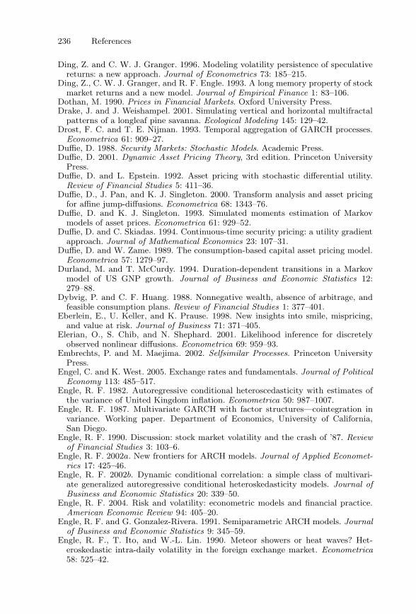
236 References

Ding, Z. and C. W. J. Granger. 1996. Modeling volatility persistence of speculativereturns: a new approach. Journal of Econometrics 73: 185–215.

Ding, Z., C. W. J. Granger, and R. F. Engle. 1993. A long memory property of stockmarket returns and a new model. Journal of Empirical Finance 1: 83–106.

Dothan, M. 1990. Prices in Financial Markets. Oxford University Press.Drake, J. and J. Weishampel. 2001. Simulating vertical and horizontal multifractal

patterns of a longleaf pine savanna. Ecological Modeling 145: 129–42.Drost, F. C. and T. E. Nijman. 1993. Temporal aggregation of GARCH processes.

Econometrica 61: 909–27.Duffie, D. 1988. Security Markets: Stochastic Models. Academic Press.Duffie, D. 2001. Dynamic Asset Pricing Theory, 3rd edition. Princeton University

Press.Duffie, D. and L. Epstein. 1992. Asset pricing with stochastic differential utility.

Review of Financial Studies 5: 411–36.Duffie, D., J. Pan, and K. J. Singleton. 2000. Transform analysis and asset pricing

for affine jump-diffusions. Econometrica 68: 1343–76.Duffie, D. and K. J. Singleton. 1993. Simulated moments estimation of Markov

models of asset prices. Econometrica 61: 929–52.Duffie, D. and C. Skiadas. 1994. Continuous-time security pricing: a utility gradient

approach. Journal of Mathematical Economics 23: 107–31.Duffie, D. and W. Zame. 1989. The consumption-based capital asset pricing model.

Econometrica 57: 1279–97.Durland, M. and T. McCurdy. 1994. Duration-dependent transitions in a Markov

model of US GNP growth. Journal of Business and Economic Statistics 12:279–88.

Dybvig, P. and C. F. Huang. 1988. Nonnegative wealth, absence of arbitrage, andfeasible consumption plans. Review of Financial Studies 1: 377–401.

Eberlein, E., U. Keller, and K. Prause. 1998. New insights into smile, mispricing,and value at risk. Journal of Business 71: 371–405.

Elerian, O., S. Chib, and N. Shephard. 2001. Likelihood inference for discretelyobserved nonlinear diffusions. Econometrica 69: 959–93.

Embrechts, P. and M. Maejima. 2002. Selfsimilar Processes. Princeton UniversityPress.

Engel, C. and K. West. 2005. Exchange rates and fundamentals. Journal of PoliticalEconomy 113: 485–517.

Engle, R. F. 1982. Autoregressive conditional heteroscedasticity with estimates ofthe variance of United Kingdom inflation. Econometrica 50: 987–1007.

Engle, R. F. 1987. Multivariate GARCH with factor structures—cointegration invariance. Working paper. Department of Economics, University of California,San Diego.

Engle, R. F. 1990. Discussion: stock market volatility and the crash of ’87. Reviewof Financial Studies 3: 103–6.

Engle, R. F. 2002a. New frontiers for ARCH models. Journal of Applied Economet-rics 17: 425–46.

Engle, R. F. 2002b. Dynamic conditional correlation: a simple class of multivari-ate generalized autoregressive conditional heteroskedasticity models. Journal ofBusiness and Economic Statistics 20: 339–50.

Engle, R. F. 2004. Risk and volatility: econometric models and financial practice.American Economic Review 94: 405–20.

Engle, R. F. and G. Gonzalez-Rivera. 1991. Semiparametric ARCH models. Journalof Business and Economic Statistics 9: 345–59.

Engle, R. F., T. Ito, and W.-L. Lin. 1990. Meteor showers or heat waves? Het-eroskedastic intra-daily volatility in the foreign exchange market. Econometrica58: 525–42.

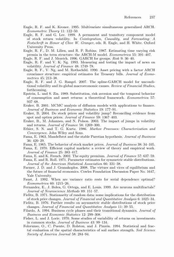
References 237

Engle, R. F. and K. Kroner. 1995. Multivariate simultaneous generalized ARCH.Econometric Theory 11: 122–50.

Engle, R. F. and G. Lee. 1999. A permanent and transitory component modelof stock return volatility. In Cointegration, Causality, and Forecasting: AFestschrift in Honor of Clive W. Granger, eds. R. Engle, and H. White. OxfordUniversity Press.

Engle, R. F., D. M. Lilien, and R. P. Robins. 1987. Estimating time varying riskpremia in the term structure: the ARCH-M model. Econometrica 55: 391–407.

Engle, R. F. and J. Mezrich. 1996. GARCH for groups. Risk 9: 36–40.Engle, R. F. and V. K. Ng. 1993. Measuring and testing the impact of news on

volatility. Journal of Finance 48: 1749–78.Engle, R. F., V. Ng, and M. Rothschild. 1990. Asset pricing with a factor ARCH

covariance structure: empirical estimates for Treasury bills. Journal of Econo-metrics 45: 213–38.

Engle, R. F. and J. G. Rangel. 2007. The spline-GARCH model for uncondi-tional volatility and its global macroeconomic causes. Review of Financial Studies,forthcoming.

Epstein, L. and S. Zin. 1989. Substitution, risk aversion and the temporal behaviorof consumption and asset returns: a theoretical framework. Econometrica 57:937–68.

Eraker, B. 2001. MCMC analysis of diffusion models with applications to finance.Journal of Business and Economic Statistics 19: 177–91.

Eraker, B. 2004. Do stock prices and volatility jump? Reconciling evidence fromspot and option prices. Journal of Finance 59: 1367–403.

Eraker, B., M. Johannes, and N. Polson. 2003. The impact of jumps in volatilityand returns. Journal of Finance 58: 1269–300.

Ethier, S. N. and T. G. Kurtz. 1986. Markov Processes: Characterization andConvergence. John Wiley and Sons.

Fama, E. 1963. Mandelbrot and the stable Paretian hypothesis. Journal of Business36: 420–29.

Fama, E. 1965. The behavior of stock market prices. Journal of Business 38: 34–105.Fama, E. 1970. Efficient capital markets: a review of theory and empirical work.

Journal of Finance 25: 383–417.Fama, E. and K. French. 2002. The equity premium. Journal of Finance 57: 637–59.Fama, E. and R. Roll. 1971. Parameter estimates for symmetric stable distributions.

Journal of the American Statistical Association 66: 331–38.Farmer, J. D. and J. Geanakoplos. 2008. The virtues and vices of equilibrium and

the future of financial economics. Cowles Foundation Discussion Paper No. 1647,Yale University.

Faust, J. 1992. When are variance ratio rests for serial dependence optimal?Econometrica 60: 1215–26.

Fernandez, E., J. Bolea, G. Ortega, and E. Louis. 1999. Are neurons multifractals?Journal of Neuroscience Methods 89: 151–57.

Fielitz, B. 1971. Stationarity of random data: some implications for the distributionof stock price changes. Journal of Financial and Quantitative Analysis 6: 1025–34.

Fielitz, B. 1976. Further results on asymmetric stable distributions of stock pricechanges. Journal of Financial and Quantitative Analysis 11: 39–55.

Filardo, A. 1994. Business cycle phases and their transitional dynamics. Journal ofBusiness and Economic Statistics 12: 299–308.

Fisher, L. and J. Lorie. 1970. Some studies of variability of returns on investmentsin common stocks. Journal of Business 43: 99–134.

Folorunso, O., C. Puente, D. Rolston, and J. Pinzon. 1994. Statistical and frac-tal evaluation of the spatial characteristics of soil surface strength. Soil ScienceSociety of America Journal 58: 284–94.

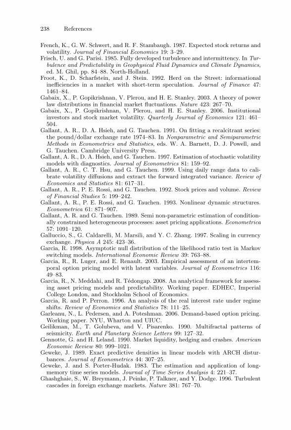
238 References

French, K., G. W. Schwert, and R. F. Stambaugh. 1987. Expected stock returns andvolatility. Journal of Financial Economics 19: 3–29.

Frisch, U. and G. Parisi. 1985. Fully developed turbulence and intermittency. In Tur-bulence and Predictability in Geophysical Fluid Dynamics and Climate Dynamics,ed. M. Ghil, pp. 84–88. North-Holland.

Froot, K., D. Scharfstein, and J. Stein. 1992. Herd on the Street: informationalinefficiencies in a market with short-term speculation. Journal of Finance 47:1461–84.

Gabaix, X., P. Gopikrishnan, V. Plerou, and H. E. Stanley. 2003. A theory of powerlaw distributions in financial market fluctuations. Nature 423: 267–70.

Gabaix, X., P. Gopikrishnan, V. Plerou, and H. E. Stanley. 2006. Institutionalinvestors and stock market volatility. Quarterly Journal of Economics 121: 461–504.

Gallant, A. R., D. A. Hsieh, and G. Tauchen. 1991. On fitting a recalcitrant series:the pound/dollar exchange rate 1974–83. In Nonparametric and SemiparametricMethods in Econometrics and Statistics, eds. W. A. Barnett, D. J. Powell, andG. Tauchen. Cambridge University Press.

Gallant, A. R., D. A. Hsieh, and G. Tauchen. 1997. Estimation of stochastic volatilitymodels with diagnostics. Journal of Econometrics 81: 159–92.

Gallant, A. R., C. T. Hsu, and G. Tauchen. 1999. Using daily range data to cali-brate volatility diffusions and extract the forward integrated variance. Review ofEconomics and Statistics 81: 617–31.

Gallant, A. R., P. E. Rossi, and G. Tauchen. 1992. Stock prices and volume. Reviewof Financial Studies 5: 199–242.

Gallant, A. R., P. E. Rossi, and G. Tauchen. 1993. Nonlinear dynamic structures.Econometrica 61: 871–907.

Gallant, A. R. and G. Tauchen. 1989. Semi non-parametric estimation of condition-ally constrained heterogeneous processes: asset pricing applications. Econometrica57: 1091–120.

Galluccio, S., G. Caldarelli, M. Marsili, and Y. C. Zhang. 1997. Scaling in currencyexchange. Physica A 245: 423–36.

Garcia, R. 1998. Asymptotic null distribution of the likelihood ratio test in Markovswitching models. International Economic Review 39: 763–88.

Garcia, R., R. Luger, and E. Renault. 2003. Empirical assessment of an intertem-poral option pricing model with latent variables. Journal of Econometrics 116:49–83.

Garcia, R., N. Meddahi, and R. Tedongap. 2008. An analytical framework for assess-ing asset pricing models and predictability. Working paper. EDHEC, ImperialCollege London, and Stockholm School of Economics.

Garcia, R. and P. Perron. 1996. An analysis of the real interest rate under regimeshifts. Review of Economics and Statistics 78: 111–25.

Garleanu, N., L. Pedersen, and A. Poteshman. 2006. Demand-based option pricing.Working paper. NYU, Wharton and UIUC.

Geilikman, M., T. Golubeva, and V. Pisarenko. 1990. Multifractal patterns ofseismicity. Earth and Planetary Science Letters 99: 127–32.

Gennotte, G. and H. Leland. 1990. Market liquidity, hedging and crashes. AmericanEconomic Review 80: 999–1021.

Geweke, J. 1989. Exact predictive densities in linear models with ARCH distur-bances. Journal of Econometrics 44: 307–25.

Geweke, J. and S. Porter-Hudak. 1983. The estimation and application of long-memory time series models. Journal of Time Series Analysis 4: 221–37.

Ghashghaie, S., W. Breymann, J. Peinke, P. Talkner, and Y. Dodge. 1996. Turbulentcascades in foreign exchange markets. Nature 381: 767–70.

References 239

Ghysels, E., A. Harvey, and E. Renault. 1996. Stochastic Volatility. In Handbook ofStatistics, eds. G. S. Maddala, and C. R. Rao, 14: 119–91. North-Holland.

Ghysels, E., P. Santa-Clara, and R. Valkanov. 2005. There is a risk-return trade-offafter all. Journal of Financial Economics 76: 509–48.

Gilbert, A., W. Willinger, and A. Feldmann. 1999. Scaling analysis of conservativecascades, with applications to network traffic. IEEE Transactions on InformationTheory 45: 971–91.

Glosten, L., R. Jagannathan, and D. Runkle. 1993. On the relation between theexpected value and the volatility of the nominal excess return on stocks. Journalof Finance 48: 1779–801.

Godano, C. and V. Caruso. 1995. Multifractal analysis of earthquake catalogues.Geophysical Journal International 121: 385–92.

Goncalves, M. 2001. Characterization of geochemical distributions using multifractalmodels. Mathematical Geology 33: 41–61.

Goncalves da Silva, A. and P. M. Robinson. 2007. Fractional cointegration instochastic volatility models. Econometric Theory, forthcoming.

Gourieroux, C. and J. Jasiak. 2002. Nonlinear autocorrelograms: an application tointer-trade durations. Journal of Time Series Analysis 23: 127–54.

Gourieroux, C. and A. Montfort. 1992. Qualitative threshold ARCH models. Journalof Econometrics 52: 159–99.

Grandmont, J. M. 1998. Expectations formation and stability of large socioeconomicsystems. Econometrica 66: 741–81.

Granger, C. W. J. 1980. Long-memory relationships and the aggregation of dynamicmodels. Journal of Econometrics 14: 227–38.

Granger, C. W. J. and N. Hyung. 1999. Occasional structural breaks and longmemory. Discussion paper 99–14, University of California, San Diego.

Granger, C. W. J. and R. Joyeux. 1980. An introduction to long memory time seriesmodels and fractional differencing. Journal of Time Series Analysis 1: 15–29.

Granger, C. W. J. and O. Morgenstern. 1970. Predictability of Stock Market Prices.Heath-Lexington, Lexington, MA.

Gray, S. 1996. Modeling the conditional distribution of interest rates as a regime-switching process. Journal of Financial Economics 42: 27–62.

Greenspan, A. 2007. The Age of Turbulence: Adventures in a New World. PenguinPress.

Greenwood, J. and B. Jovanovic. 1999. The information-technology revolution andthe stock market. American Economic Review 89: 116–22.

Grout, H., A. Tarquis, and M. Wiesner. 1998. Multifractal analysis of particle sizedistributions in soil. Environmental Science and Technology 32: 1176–82.

Guidolin, M. and A. Timmermann. 2003. Option prices under Bayesian learning:implied volatility dynamics and predictive densities. Journal of Economic Dynam-ics and Control 27: 717–69.

Guivarc’h, Y. 1987. Remarques sur les solutions d’une equation fonctionnelle nonlineaire de Benoıt Mandelbrot. Comptes Rendus de l’Academie des Sciences deParis 3051: 139.

Gutierrez, J., M. Rodriguez, and G. Abramson. 2001. Multifractal analysis of DNAsequences using a novel chaos-game representation. Physica A 300: 271–84.

Hall, P. 1982. On some simple estimates of an exponent of regular variations. Journalof the Royal Statistical Society Series B 44: 37–42.

Halsey, T. C., M. H. Jensen, L. P. Kadanoff, I. Procaccia, and B. I. Shraiman.1986. Fractal measures and their singularities: the characterization of strangesets. Physical Review Letters A 33: 1141.

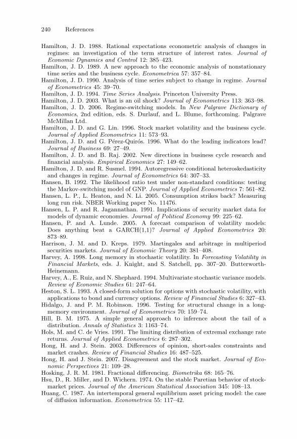
240 References

Hamilton, J. D. 1988. Rational expectations econometric analysis of changes inregimes: an investigation of the term structure of interest rates. Journal ofEconomic Dynamics and Control 12: 385–423.

Hamilton, J. D. 1989. A new approach to the economic analysis of nonstationarytime series and the business cycle. Econometrica 57: 357–84.

Hamilton, J. D. 1990. Analysis of time series subject to change in regime. Journalof Econometrics 45: 39–70.

Hamilton, J. D. 1994. Time Series Analysis. Princeton University Press.Hamilton, J. D. 2003. What is an oil shock? Journal of Econometrics 113: 363–98.Hamilton, J. D. 2006. Regime-switching models. In New Palgrave Dictionary of

Economics, 2nd edition, eds. S. Durlauf, and L. Blume, forthcoming. PalgraveMcMillan Ltd.

Hamilton, J. D. and G. Lin. 1996. Stock market volatility and the business cycle.Journal of Applied Econometrics 11: 573–93.

Hamilton, J. D. and G. Perez-Quiros. 1996. What do the leading indicators lead?Journal of Business 69: 27–49.

Hamilton, J. D. and B. Raj. 2002. New directions in business cycle research andfinancial analysis. Empirical Economics 27: 149–62.

Hamilton, J. D. and R. Susmel. 1994. Autoregressive conditional heteroskedasticityand changes in regime. Journal of Econometrics 64: 307–33.

Hansen, B. 1992. The likelihood ratio test under non-standard conditions: testingthe Markov-switching model of GNP. Journal of Applied Econometrics 7: 561–82.

Hansen, L. P., L. Heaton, and N. Li. 2005. Consumption strikes back? Measuringlong run risk. NBER Working paper No. 11476.

Hansen, L. P. and R. Jagannathan. 1991. Implications of security market data formodels of dynamic economies. Journal of Political Economy 99: 225–62.

Hansen, P. and A. Lunde. 2005. A forecast comparison of volatility models:Does anything beat a GARCH(1,1)? Journal of Applied Econometrics 20:873–89.

Harrison, J. M. and D. Kreps. 1979. Martingales and arbitrage in multiperiodsecurities markets. Journal of Economic Theory 20: 381–408.

Harvey, A. 1998. Long memory in stochastic volatility. In Forecasting Volatility inFinancial Markets, eds. J. Knight, and S. Satchell, pp. 307–20. Butterworth-Heinemann.

Harvey, A., E. Ruiz, and N. Shephard. 1994. Multivariate stochastic variance models.Review of Economic Studies 61: 247–64.

Heston, S. L. 1993. A closed-form solution for options with stochastic volatility, withapplications to bond and currency options. Review of Financial Studies 6: 327–43.

Hidalgo, J. and P. M. Robinson. 1996. Testing for structural change in a long-memory environment. Journal of Econometrics 70: 159–74.

Hill, B. M. 1975. A simple general approach to inference about the tail of adistribution. Annals of Statistics 3: 1163–74.

Hols, M. and C. de Vries. 1991. The limiting distribution of extremal exchange ratereturns. Journal of Applied Econometrics 6: 287–302.

Hong, H. and J. Stein. 2003. Differences of opinion, short-sales constraints andmarket crashes. Review of Financial Studies 16: 487–525.

Hong, H. and J. Stein. 2007. Disagreement and the stock market. Journal of Eco-nomic Perspectives 21: 109–28.

Hosking, J. R. M. 1981. Fractional differencing. Biometrika 68: 165–76.Hsu, D., R. Miller, and D. Wichern. 1974. On the stable Paretian behavior of stock-

market prices. Journal of the American Statistical Association 345: 108–13.Huang, C. 1987. An intertemporal general equilibrium asset pricing model: the case

of diffusion information. Econometrica 55: 117–42.

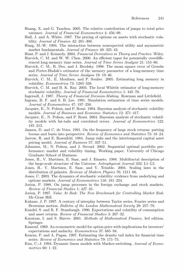
References 241

Huang, X. and G. Tauchen. 2005. The relative contribution of jumps to total pricevariance. Journal of Financial Econometrics 4: 456–99.

Hull, J. and A. White. 1987. The pricing of options on assets with stochastic vola-tility. Journal of Finance 42: 281–300.

Hung, M.-W. 1994. The interaction between nonexpected utility and asymmetricmarket fundamentals. Journal of Finance 49: 325–43.

Hunt, P. and J. Kennedy. 2004. Financial Derivatives in Theory and Practice. Wiley.Hurvich, C. M. and W. W. Chen. 2000. An efficient taper for potentially overdiffe-

renced long-memory time series. Journal of Time Series Analysis 21: 155–80.Hurvich, C. M., R. Deo, and J. Brodsky. 1998. The mean square error of Geweke

and Porter-Hudak’s estimator of the memory parameter of a long-memory timeseries. Journal of Time Series Analysis 19: 19–46.

Hurvich, C. M., E. Moulines, and P. Soulier. 2005. Estimating long memory involatility. Econometrica 73: 1283–328.

Hurvich, C. M. and B. K. Ray. 2003. The local Whittle estimator of long-memorystochastic volatility. Journal of Financial Econometrics 1: 445–70.

Ingersoll, J. 1987. Theory of Financial Decision-Making. Rowman and Littlefield.Ingram, B. F. and S. B. Lee. 1991. Simulation estimation of time series models.

Journal of Econometrics 47: 197–250.Jacquier, E., N. Polson, and P. Rossi. 1994. Bayesian analysis of stochastic volatility

models. Journal of Business and Economic Statistics 12: 371–417.Jacquier, E., N. Polson, and P. Rossi. 2004. Bayesian analysis of stochastic volatil-

ity models with fat-tails and correlated errors. Journal of Econometrics 122:185–212.

Jansen, D. and C. de Vries. 1991. On the frequency of large stock returns: puttingbooms and busts into perspective. Review of Economics and Statistics 73: 18–24.

Jarrow, R. and E. Rosenfeld. 1984. Jump risks and the intertemporal capital assetpricing model. Journal of Business 57: 337–51.

Johannes, M., N. Polson, and J. Stroud. 2002. Sequential optimal portfolio per-formance: market and volatility timing. Working paper. University of ChicagoGraduate School of Business.

Jones, B., V. Martinez, E. Saar, and J. Einasto. 1988. Multifractal description ofthe large-scale structure of the Universe. Astrophysical Journal 332: L1–L5.

Jones, B., V. Martinez, E. Saar, and V. Trimble. 2004. Scaling laws in thedistribution of galaxies. Reviews of Modern Physics 76: 1211–66.

Jones, C. 2003. The dynamics of stochastic volatility: evidence from underlying andoptions markets. Journal of Econometrics 116: 181–224.

Jorion, P. 1988. On jump processes in the foreign exchange and stock markets.Review of Financial Studies 1: 427–45.

Jorion, P. 1997. Value At Risk: The New Benchmark for Controlling Market Risk.Mc-Graw Hill.

Kahane, J. P. 1997. A century of interplay between Taylor series, Fourier series andBrownian motion. Bulletin of the London Mathematical Society 29: 257–79.

Kandel, S. and R. F. Stambaugh. 1990. Expectations and volatility of consumptionand asset returns. Review of Financial Studies 3: 207–32.

Karatzas, I. and S. Shreve. 2001. Methods of Mathematical Finance, 3rd edition.Springer.

Kassouf. 1969. An econometric model for option price with implications for investors’expectations and audacity. Econometrica 37: 685–94.

Kearns, P. and A. Pagan. 1997. Estimating the density tail index for financial timeseries. Review of Economics and Statistics 79: 171–75.

Kim, C.-J. 1994. Dynamic linear models with Markov-switching. Journal of Econo-metrics 60: 1–22.

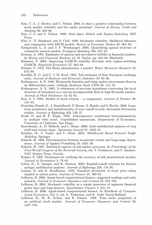
242 References

Kim, C.-J., J. Morley, and C. Nelson. 2004. Is there a positive relationship betweenstock market volatility and the equity premium? Journal of Money, Credit andBanking 36: 339–60.

Kim, C.-J. and C. Nelson. 1999. State-Space Models with Regime-Switching. MITPress.

Kim, S., N. Shephard, and S. Chib. 1998. Stochastic volatility: likelihood inferenceand comparison with ARCH models. Review of Economic Studies 65: 361–93.

Kirkpatrick, L. A. and J. F. Weishampel. 2005. Quantifying spatial structure ofvolumetric neutral models. Ecological Modeling 186: 312–25.

Kirman, A. 1991. Epidemics of opinion and speculative bubbles in financial markets.In Money and Financial Markets, ed. M. Taylor, pp. 354–68. Blackwell.

Klaassen, F. 2002. Improving GARCH volatility forecasts with regime-switchingGARCH. Empirical Economics 27: 363–94.

Klemes, V. 1974. The Hurst phenomenon: a puzzle? Water Resources Research 10:675–88.

Koedjik, K. G. and C. J. M. Kool. 1992. Tail estimates of East European exchangerates. Journal of Business and Economic Statistics 10: 83–96.

Kolmogorov, A. N. 1940. Wienersche Spiralen und einige andere interessante Kurvenim Hilbertschen raum. Doklady Akademii Nauk USSR 26: 115–18.

Kolmogorov, A. N. 1962. A refinement of previous hypotheses concerning the localstructure of turbulence in a viscous incompressible fluid at high Reynolds number.Journal of Fluid Mechanics 13: 82–85.

Kon, S. J. 1984. Models of stock returns – a comparison. Journal of Finance 39:147–65.

Koscielny-Bunde, E., J. Kantelhardt, P. Braun, A. Bunde, and S. Havlin. 2006. Long-term persistence and multifractality of river runoff records: detrended fluctuationstudies. Journal of Hydrology 322: 120–37.

Kraft, D. and R. F. Engle. 1982. Autoregressive conditional heteroskedasticityin multiple time series. Unpublished manuscript, Department of Economics,University of California, San Diego.

Kravchenko, A., D. Bullock, and C. Boast. 2000. Joint multifractal analyses of cropyield and terrain slope. Agronomy Journal 91: 1033–41.

Krishna, M., V. Gadre, and U. Desai. 2003. Multifractal Based Network TrafficModeling. Springer.

Kunsch, H. 1986. Discrimination between monotonic trends and long-range depen-dence. Journal of Applied Probability 23: 1025–30.

Kunsch, H. 1987. Statistical aspects of self-similar processes. In Proceedings of theFirst World Congress of the Bernoulli Society, eds. Y. Prokhorov, and V. Sasanov.VNU Science Press, Utrecht.

Kupiec, P. 1995. Techniques for verifying the accuracy of risk measurement models.Journal of Derivatives 2: 73–84.

Labat, D., A. Mangin, and R. Ababou. 2002. Rainfall-runoff relations for Karsticsprings: multifractal analyses. Journal of Hydrology 256: 176–95.

Latane, H. and R. Rendleman. 1976. Standard deviations of stock price ratiosimplied in option prices. Journal of Finance 31: 369–81.

LeBaron, B. 2000. Agent-based computational finance: suggested readings and earlyresearch. Journal of Economic Dynamics and Control 24: 679–702.

LeBaron, B. 2001. Stochastic volatility as a simple generator of apparent financialpower laws and long memory. Quantitative Finance 1: 621–31.

LeBaron, B. 2006. Agent-based computational finance. In Handbook of Computa-tional Economics, Vol. 2, eds. L. Tesfatsion, and K. Judd. North-Holland.

LeBaron, B., W. B. Arthur, and R. Palmer. 1999. Time series properties ofan artificial stock market. Journal of Economic Dynamics and Control 23:1487–516.

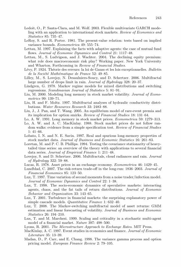
References 243

Ledoit, O., P. Santa-Clara, and M. Wolf. 2003. Flexible multivariate GARCH mode-ling with an application to international stock markets. Review of Economics andStatistics 85: 735–47.

LeRoy, S. and R. Porter. 1981. The present-value relation: tests based on impliedvariance bounds. Econometrica 49: 555–74.

Lettau, M. 1997. Explaining the facts with adaptive agents: the case of mutual fundflows. Journal of Economic Dynamics and Control 21: 1117–48.

Lettau, M., S. Ludvigson, and J. Wachter. 2004. The declining equity premium:what role does macroeconomic risk play? Working paper. New York Universityand Wharton. Forthcoming in Review of Financial Studies.

Levy, P. 1924. Theorie des erreurs: la loi de Gauss et les lois exceptionnelles. Bulletinde la Societe Mathematique de France 52: 49–85.

Lilley, M., S. Lovejoy, N. Desaulniers-Soucy, and D. Schertzer. 2006. Multifractallarge number of drops limit in rain. Journal of Hydrology 328: 20–37.

Lindgren, G. 1978. Markov regime models for mixed distributions and switchingregressions. Scandinavian Journal of Statistics 5: 81–91.

Liu, M. 2000. Modeling long memory in stock market volatility. Journal of Econo-metrics 99: 139–71.

Liu, H. and F. Moltz. 1997. Multifractal analyses of hydraulic conductivity distri-butions. Water Resources Research 33: 2483–88.

Liu, J., J. Pan, and T. Wang. 2005. An equilibrium model of rare-event premia andits implication for option smirks. Review of Financial Studies 18: 131–64.

Lo, A. W. 1991. Long memory in stock market prices. Econometrica 59: 1279–313.Lo, A. W. and A. C. MacKinlay. 1988. Stock market prices do not follow ran-

dom walks: evidence from a simple specification test. Review of Financial Studies1: 41–66.

Lobato, I. N. and N. E. Savin. 1997. Real and spurious long-memory properties ofstock market data. Journal of Business and Economic Statistics 16: 261–83.

Loretan, M. and P. C. B. Phillips. 1994. Testing the covariance stationarity of heavy-tailed time series: an overview of the theory with applications to several financialdata series. Journal of Empirical Finance 1: 211–48.

Lovejoy, S. and D. Schertzer. 2006. Multifractals, cloud radiances and rain. Journalof Hydrology 322: 59–88.

Lucas, R. 1978. Asset prices in an exchange economy. Econometrica 46: 1429–45.Lundblad, C. 2007. The risk-return trade-off in the long-run: 1836–2003. Journal of

Financial Economics 85: 123–50.Lux, T. 1997. Time variation of second moments from a noise trader/infection model.

Journal of Economic Dynamics and Control 22: 1–38.Lux, T. 1998. The socio-economic dynamics of speculative markets: interacting

agents, chaos, and the fat tails of return distributions. Journal of EconomicBehavior and Organization 33: 143–65.

Lux, T. 2001. Turbulence in financial markets: the surprising explanatory power ofsimple cascade models. Quantitative Finance 1: 632–40.

Lux, T. 2008. The Markov-switching multifractal model of asset returns: GMMestimation and linear forecasting of volatility. Journal of Business and EconomicStatistics 26: 194–210.

Lux, T. and M. Marchesi. 1999. Scaling and criticality in a stochastic multi-agentmodel of a financial market. Nature 397: 498–500.

Lyons, R. 2001. The Microstructure Approach to Exchange Rates. MIT Press.MacKinlay, A. C. 1997. Event studies in economics and finance. Journal of Economic

Literature 35: 13–39.Madan, D., P. Carr, and E. Chang. 1998. The variance gamma process and option

pricing model. European Finance Review 2: 79–105.

244 References

Maheswaran, S. and C. Sims. 1993. Empirical implications of arbitrage-free assetmarkets. In Models, Methods and Applications of Econometrics, ed. P. C. B.Phillips. Basil Blackwell.

Maheu, J. and T. McCurdy. 2000. Volatility dynamics under duration-dependentmixing. Journal of Empirical Finance 7: 345–72.

Maheu, J. and T. McCurdy. 2004. News arrival, jump dynamics, and volatilitycomponents for individual stock returns. Journal of Finance 59: 755–93.

Mandelbrot, B. B. 1963. The variation of certain speculative prices. Journal ofBusiness 36: 394–419.

Mandelbrot, B. B. 1965a. Une classe de processus stochastiques homothetiques asoi. Comptes Rendus de l’Academie des Sciences de Paris 260: 3274–77.

Mandelbrot, B. B. 1965b. Time varying channels, 1/f noises and the infrared catas-trophe, or: why does the low frequency energy sometimes seem infinite. ConferenceRecord of the 1st IEEE Annual Communications Convention, Boulder, Colorado.

Mandelbrot, B. B. 1967. The variation of some other speculative prices. Journal ofBusiness 40: 393–413.

Mandelbrot, B. B. 1972. Possible refinement of the lognormal hypothesis concerningthe distribution of energy dissipation in intermittent turbulence. In StatisticalModels and Turbulence, Lecture Note in Physics, eds. M. Rosenblatt, and C. VanAtta, 12: 333–51. Springer.

Mandelbrot, B. B. 1974. Intermittent turbulence in self-similar cascades: divergenceof high moments and dimension of the carrier. Journal of Fluid Mechanics 62:331–58.

Mandelbrot, B. B. 1982. The Fractal Geometry of Nature. Freeman.Mandelbrot, B. B. 1989. Multifractal measures, especially for the geophysicist. Pure

and Applied Geophysics 131: 5–42.Mandelbrot, B. B. 1997. Fractals and Scaling in Finance. Springer.Mandelbrot, B. B. 1999. Multifractals and 1/f Noise: Wild Self-Affinity in Physics.

Springer.Mandelbrot, B. B. 2001. Stochastic volatility, power laws, and long-memory. Quanti-

tative Finance 1: 558–59.Mandelbrot, B. B. and R. Hudson. 2004. The (Mis) behavior of Markets. Basic

Books.Mandelbrot, B. B. and H. W. Taylor. 1967. On the distribution of stock price

differences. Operations Research 15: 1057–62.Mandelbrot, B. B. and J. W. van Ness. 1968. Fractional Brownian motion, fractional

noises and application. SIAM Review 10: 422–37.Mantegna, R. and H. E. Stanley. 1996. Turbulence and financial markets. Nature

383: 587–88.Mantegna, R. and H. E. Stanley. 2000. An Introduction to Econophysics: Correla-

tions and Complexity in Finance. Cambridge University Press.Martin, M. and E. Montero. 2002. Laser diffraction and multifractal analysis for the

characterization of dry soil volume-size distributions. Soil & Tillage Research 64:113–23.

Martinez, V. 1999. Is the universe fractal? Science 284: 445–46.McCurdy, T. and I. Morgan. 1987. Tests of the martingale hypothesis for foreign

currency futures with time varying volatility. International Journal of Forecasting3: 131–48.

Meese, R. and K. Rogoff. 1983. Empirical exchange rate models of the seventies: dothey fit out of sample? Journal of International Economics 14: 3–24.

Mehra, R. and E. C. Prescott. 1985. The equity premium: a puzzle. Journal ofMonetary Economics 15: 145–61.

Melino, A. and S. M. Turnbull. 1990. Pricing foreign currency options with stochasticvolatility. Journal of Econometrics 45: 239–65.

References 245

Meneveau, C. and K. Sreenivasan. 1987. Simple multifractal cascade model for fullydeveloped turbulence. Physical Review Letters 59: 1424–27.

Meneveau, C. and K. Sreenivasan. 1991. The multifractal nature of turbulent energydissipation. Journal of Fluid Mechanics 224: 429–84.

Merton, R. 1973. Rational theory of option pricing. Bell Journal of Economics andManagement Science 4: 141–83.

Merton, R. C. 1976. Option pricing when underlying stock returns are discontinuous.Journal of Financial Economics 3: 125–44.

Merton, R. C. 1990. Continuous-Time Finance. Cambridge, Massachusetts, Black-well.

Milhoj, A. 1987. A conditional variance model for daily deviations of an exchangerate. Journal of Business and Economic Statistics 5: 99–103.

Mincer, J. and V. Zarnowitz. 1969. The evaluation of economic forecasts. In Eco-nomic Forecasts and Expectations, ed. J. Mincer. National Bureau of EconomicResearch, New York.

Molchan, G. and T. Kronrod. 2007. Seismic interevent time: a spatial scaling andmultifractality. Pure and Applied Geophysics 164: 75–96.

Muller, U., M. Dacorogna, R. Dave, O. Pictet, R. Olsen, and J. Ward. 1995. Fractalsand intrinsic time: a challenge to econometricians. Discussion Paper Presented atthe 1993 International Conference of the Applied Econometrics Association heldin Luxembourg.

Muller, U., M. Dacorogna, R. Olsen, O. Pictet, M. Schwarz, and C. Morgenegg.1990. Statistical study of foreign exchange rates, empirical evidence of a pricechange scaling law, and intraday analysis. Journal of Banking and Finance 14:1189–1208.

Musiela, M. and M. Rutkowski. 2007. Martingale Methods in Financial Modeling.2nd edition. Springer.

Muzy, J.-F. and E. Bacry. 2002. Multifractal stationary random measures and mul-tifractal random walks with log infinitely divisible scaling laws. Physical ReviewE 66: 056121.

Muzy, J.-F., E. Bacry, and A. Arneodo. 1991. Wavelets and multifractal formalismfor singular signals: application to turbulence data. Physical Review Letters 67:3515–18.

Muzy, J.-F., J. Delour, and E. Bacry. 2000. Modeling fluctuations of financial timeseries: from cascade process to stochastic volatility model. European PhysicalJournal B 17: 537–48.

Naik, V. and M. Lee. 1990. General equilibrium pricing of options on the marketportfolio with discontinuous returns. Review of Financial Studies 3: 493–521.

Nakaya, S. and T. Hashimoto. 2002. Temporal variation of multifractal properties ofseismicity in the region affected by the mainshock of the October 6, 2000 WesternTottori Prefecture, Japan, earthquake (M = 7.3). Geophysical Research Letters29(10): 1–4.

Neftci, S. 2000. Introduction to the Mathematics of Financial Derivatives, 2ndedition. Academic Press.

Nelson, D. 1989. Modeling stock market volatility changes. Proceedings from theAmerican Statistical Association, Business and Economics Statistics Section,93–98.

Nelson, D. 1990. ARCH models as diffusion aproximations. Journal of Econometrics45: 7–38.

Nelson, D. 1991. Conditional heteroskedasticity in asset returns: a new approach.Econometrica 45: 7–38.

Newey, W. and K. West. 1987. A simple, positive semi-definite, heteroskedasticityand autocorrelation consistent covariance matrix. Econometrica 55: 703–8.

246 References

Newey, W. and K. West. 1994. Automatic lag selection in covariance matrixestimation. Review of Economic Studies 61: 631–54.

Nicolato, E. and E. Venardos. 2003. Option pricing in stochastic volatility modelsof the Ornstein-Uhlenbeck type. Mathematical Finance 13: 445–66.

Nielsen, L. T. 1999. Pricing and Hedging of Derivative Securities. Oxford UniversityPress.

Nijman, T. and F. Palm. 1993. GARCH modeling of volatility: an introduction totheory and applications. In Advanced Lectures in Quantitative Economics, ed.A. J. de Zeeuw. Academic Press.

Officer, R. 1972. The distribution of stock returns. Journal of the AmericanStatistical Association 67: 807–12.

Officer, R. 1973. The variability of the market factor of the New York StockExchange. Journal of Business 46: 434–53.

Olsson, J. and J. Niemczynowicz. 1996. Multifractal analysis of daily spatial rainfalldistributions. Journal of Hydrology 187: 29–43.

Oprisan, S., A. Ardelean, and P. Frangopol. 2000. Self-organization and competitionin the immune response to cancer invasion: a phase-oriented computational modelof oncogenesis. Bioinformatics 16: 96–100.

Osborne, M. 1962. Periodic structure in the Brownian motion of stock prices.Operations Research 10: 345–79.

Pagan, A. and Y. Hong. 1991. Nonparametric estimation and the risk premium.In Nonparametric and Semiparametric Methods in Econometrics and Statistics,eds. W. A., Barnett, D. J. Powell, and G. Tauchen. Cambridge UniversityPress.

Pagan, A. and W. Schwert. 1990. Alternative models for conditional stock volatility.Journal of Econometrics 45: 267–90.

Pan, J. 2002. The jump-risk premia implicit in options: evidence from an integratedtime-series study. Journal of Financial Economics 63: 3–50.

Pandey, G., S. Lovejoy, and D. Schertzer. 1998. Multifractal analysis of daily riverflows including extremes for basins of five to two million square kilometers, oneday to seventy-five years. Journal of Hydrology 208: 62–81.

Paredes, C. and F. Elorza. 1999. Fractal and multifractal analysis of fracturedgeological media: surface-subsurface correlation. Computers and Geosciences 25:1081–96.

Pasquini, M. and M. Serva. 1999. Multiscale behavior of volatility autocorrelationsin a financial market. Economics Letters 65: 275–79.

Pasquini, M. and M. Serva. 2000. Clustering of volatility as a multiscale pheno-menon. European Physical Journal B 16: 195–201.

Pastor, L. and P. Veronesi. 2008. Technological revolutions and stock prices. Workingpaper. University of Chicago.

Perez-Quiros, G. and A. Timmermann. 2000. Firm size and cyclical variations instock returns. Journal of Finance 55: 1229–62.

Peyriere, J. 1991. Multifractal measures. In Proceedings of the NATO ASI “Proba-bilistic Stochastic Methods in Analysis, with Applications.”

Phillips, P. C. B. 1999. Discrete Fourier transforms of fractional processes. CowlesFoundation Discussion Paper no. 1243, Yale University.

Phillips, P. C. B., J. W. McFarland, and P. C. McMahon. 1996. Robust tests of for-ward exchange market efficiency with empirical evidence from the 1920’s. Journalof Applied Econometrics 11: 1–22.

Phillips, P. C. B. and K. Shimotsu. 2004. Local Whittle estimation in nonstationaryand unit root cases. Annals of Statistics 32: 656–92.

Pickands, J. 1975. Statistical inference using extreme order statistics. Annals ofStatistics 3: 119–31.

References 247

Pietronero, L. 1987. The fractal structure of the universe: correlations of galaxiesand clusters and the average mass density. Physica A 144: 257–84.

Pindyck, R. 1984. Risk, inflation, and the stock market. American Economic Review74: 334–51.

Pitt, M. and N. Shephard. 1999. Filtering via simulation: auxiliary particle filter.Journal of the American Statistical Association 94: 590–99.

Pollard, D. 1984. Convergence of Stochastic Processes. Springer.Posadas, A., D. Gimenez, R. Quiroz, and R. Protz. 2003. Multifractal charac-

terization of soil pore systems. Soil Science Society of America Journal 67:1351–69.

Poterba, J. and L. Summers. 1986. The persistence of volatility and stock marketfluctuations. American Economic Review 76: 1142–51.

Praetz, P. 1969. Australian share prices and the random walk hypothesis. AustralianJournal of Statistics 11: 123–39.

Praetz, P. 1972. The distribution of share price changes. Journal of Business 45:49–55.

Press, S. J. 1967. A compound events model for security prices. Journal of Business40: 317–35.

Quintos, C., Z. Fan, and P. C. B. Phillips. 2001. Structural change tests in tailbehavior and the Asian crisis. Review of Economic Studies 68: 633–63.

Raimondo, R. C. 2005. Market clearing, utility functions and securities prices.Economic Theory 25: 265–85.

Renault, E. and N. Touzi. 1996. Option hedging and implied volatilities in astochastic volatility model. Mathematical Finance 6: 279–302.

Richards, G. 2000. The fractal structure of exchange rates: measurement and fore-casting. Journal of International Financial Markets, Institutions and Money 10:163–80.

Richardson, M. and J. Stock. 1989. Drawing inferences from statistics based onmulti-year asset returns. Journal of Financial Economics 25: 323–48.

Riedi, R., M. Crouse, V. Ribeiro, and R. Baraniuk. 1999. A multifractal waveletmodel with application to network traffic. IEEE Transactions on InformationTheory 45: 992–1018.

Rivers, D. and Q. Vuong. 2002. Model selection tests for nonlinear dynamic models.Econometrics Journal 5(1): 1–39.

Robinson, P. M. 1978. Statistical inference for a random coefficient autoregressivemodel. Scandinavian Journal of Statistics 5: 163–68.

Robinson, P. M. 1991. Testing for strong serial correlation and dynamic conditionalheteroskedasticity in multiple regression. Journal of Econometrics 47: 67–84.

Robinson, P. M. 1995a. Log-periodogram regression of time series with long rangedependence. Annals of Statistics 23: 1048–72.

Robinson, P. M. 1995b. Gaussian semiparametric estimation of long range depen-dence. Annals of Statistics 23: 1630–61.

Robinson, P. M. 2001. The memory of stochastic volatility models. Journal ofEconometrics 101: 195–218.

Robinson, P. M. 2003. Time Series with Long Memory. Oxford University Press.Robinson, P. M. 2005. Robust covariance matrix estimation: HAC estimates with

long memory/antipersistence correction. Econometric Theory 21: 171–80.Robinson, P. M. and P. Zaffaroni. 1998. Nonlinear time series with long memory:

a model for stochastic volatility. Journal of Statistical Planning and Inference 68:359–71.

Rogers, L. C. G. and D. Williams. 2000. Diffusions, Markov Processes and Martin-gales. Cambridge University Press.

Rogoff, K. 1999. Perspectives on exchange rate volatility. In International CapitalFlows, ed. M. Feldstein, pp. 441–53. University of Chicago Press.

248 References

Roll, R. 1984a. Orange juice and the weather. American Economic Review 74:861–80.

Roll, R. 1984b. A simple implicit measure of the effective bid-ask spread in anefficient market. Journal of Finance 39: 1127–40.

Rosenberg, B. 1972. The behavior of random variables with nonstationary varianceand the distribution of security prices. Working paper. UC Berkeley. Reprintedin Shephard (2005).

Rosenblatt, M. 1952. Remarks on a multivariate transformation. Annals of Mathe-matical Statistics 23: 470–72.

Rossi, P. 1996. Modeling Stock Market Volatility: Bridging the Gap to ContinuousTime. Academic Press.

Samorodnitsky, G. and M. S. Taqqu. 1994. Stable Non-Gaussian Random Processes.Chapman and Hall.

Samuelson, P. 1967. Efficient portfolio selection for Pareto-Levy investments.Journal of Financial and Quantitative Analysis 2: 107–22.

Samuelson, P. 1976. Limited liability, short selling, bounded utility, and infinite-variance stable distributions. Journal of Financial and Quantitative Analysis 3:485–503.

Santa-Clara, P. and R. Valkanov. 2003. The presidential puzzle: political cycles andthe stock market. Journal of Finance 58: 1841–72.

Santos, T. and P. Veronesi. 2005. Labor income and predictable stock returns.Review of Financial Studies 19: 1–44.

Sarno, L. and M. Taylor. 2002. The Economics of Exchange Rates. CambridgeUniversity Press.

Scharfstein, D. and J. Stein. 1990. Herd behavior and investment. American Econo-mic Review 80: 465–79.

Schertzer, D. and S. Lovejoy. 1987. Physical modeling and analysis of rain and cloudsby anisotropic scaling of multiplicative processes. Journal of Geophysical Research92: 9693–714.

Schmalensee, R. and R. Trippi. 1978. Common stock volatility expectations impliedby option premia. Journal of Finance 33: 129–47.

Schwert, G. W. 1989. Why does stock market volatility change over time? Journalof Finance 44: 1115–53.

Schwert, G. W. 1990a. Stock volatility and the crash of ’87. Review of FinancialStudies 3: 77–102.

Schwert, G. W. 1990b. Indexes of United States stock prices from 1802 to 1987.Journal of Business 63: 399–426.

Sentana, E. 1995. Quadratic ARCH models. Review of Economic Studies 62:639–61.

Shephard, N. 1994. Partial non-Gaussian state space. Biometrika 81: 115–31.Shephard, N. 2005. Stochastic Volatility: Selected Readings, edited volume. Oxford

University Press.Shiller, R. 1981. Do stock prices move too much to be justified by subsequent changes

in dividends? American Economic Review 71: 421–36.Shimotsu, K. and P. C. B. Phillips. 2005. Exact local Whittle estimation of fractional

integration. Annals of Statistics 33: 1890–933.Shimotsu, K. and P. C. B. Phillips. 2006. Local Whittle estimation of fractional

integration and some of its variants. Journal of Econometrics 130: 209–33.Shorack, G. and J. Wellner. 1986. Empirical Processes with Applications to Statistics.

John Wiley and Sons.Shreve, S. 2005. Stochastic Calculus for Finance. Springer.Smith, T., G. Lange, and W. Marks. 1996. Fractal methods and results in cellular

morphology – dimensions, lacunarity, and multifractals. Journal of NeuroscienceMethods 69: 123–36.

References 249

Sornette, D. 2004. Critical Phenomena in Natural Sciences. Springer.Sornette, D. and G. Ouillon. 2005. Multifractal scaling of thermally activated

rupture processes. Physical Review Letters 94: 038501, 1–4.Sowell, F. B. 1992. Modeling long run behavior with the fractional ARIMA model.

Journal of Monetary Economics 29: 277–302.Stanley, H. E. and P. Meakin. 1988. Multifractal phenomena in physics and

chemistry. Nature 335: 405–09.Stanley, H. E. and V. Plerou. 2001. Scaling and universality in economics: empirical

results and theoretical interpretation. Quantitative Finance 1: 563–67.Stein, E. M. and J. Stein. 1991. Stock price distributions with stochastic volatility:

an analytic approach. Review of Financial Studies 4: 727–52.Stock, J. H. 1987. Measuring business cycle time. Journal of Political Economy 95:

1240–61.Stock, J. H. 1988. Estimating continuous time processes subject to time deformation.

Journal of the American Statistical Association 83: 77–85.Stock, J. and M. Watson. 2003. Has the business cycle changed? Evidence and

explanations. In Monetary Policy and Uncertainty, Federal Reserve Bank ofKansas City, 9–56.

Stojic, T., I. Reljin, and B. Reljin. 2006. Adaptation of multifractal analysisto segmentation of microcalcifications in digital mammograms. Physica A 367:494–508.

Takahashi, T., T. Murata, K. Narita, T. Hamada, H. Kosaka, M. Omori, K. Taka-hashi, H. Kimura, H. Yoshida, and Y. Wada. 2004. Quantitative evaluation ofage-related white matter microstructural changes on MRI by multifractal analysis.Journal of Neurological Science 225: 33–37.

Taleb, N. 2007. The Black Swan: The Impact of the Highly Improbable. RandomHouse.

Taylor, S. J. 1982. Financial returns modelled by the product of two stochasticprocesses – a study of daily sugar prices 1961–79. In Time Series Analysis: Theoryand Practice, ed. O. D. Andesron, 1: 203–26. North-Holland.

Taylor, S. J. 1986. Modeling Financial Time Series. John Wiley and Sons.Tessier, Y., S. Lovejoy, and D. Schertzer. 1994. The multifractal global raingage

network: analysis and simulation. Journal of Applied Meteorology 32: 223–350.Teverovsky, V. and M. S. Taqqu. 1997. Testing for long-range dependence in the

presence of shifting means or a slowly-varying declining trend using a variance-type estimator. Journal of Time Series Analysis 18: 279–304.

Thompson, S. B. 2000. Specification tests for continuous time models. University ofCalifornia at Berkeley, Ph.D. Dissertation (Chapter 3).

Timmermann, A. G. 1993. How learning in financial markets generates excessvolatility and predictability in stock prices. Quarterly Journal of Economics 108:1135–45.

Timmermann, A. G. 1996. Excess volatility and predictability of stock prices inautoregressive dividend models with learning. Review of Economic Studies 63:523–57.

Tino, P. 2002. Multifractal properties of Hao’s geometric representations of DNAsequences. Physica A 304: 480–94.

Turner, C., R. Startz, and C. Nelson. 1989. A Markov model of heteroskedasticity,risk and learning in the stock market. Journal of Financial Economics 25: 3–22.

Valdarnini, R., S. Borgani, and A. Provenzale. 1992. Multifractal properties ofcosmological N-body simulations. Astrophysical Journal 394: 422–41.

van der Vaart, A. W. 1998. Asymptotic Statistics. Cambridge University Press.Vandewalle, N. and M. Ausloos. 1998. Multi-affine analysis of typical currency

exchange rates. European Physical Journal B 4: 257–61.

250 References

Vassilicos, J. C., A. Demos, and F. Tata. 1993. No evidence of chaos but someevidence of multifractals in the foreign exchange and the stock market. In Appli-cations of Fractals and Chaos, eds. A. J. Crilly, R. A. Earnshaw, and H. Jones,pp. 249–65. Springer.

Velasco, C. 1999. Gaussian semiparametric estimation of non-stationary time series.Journal of Time Series Analysis 20: 87–127.

Veronesi, P. 1999. Stock market overreaction to bad news in good times: a rationalexpectations equilibrium model. Review of Financial Studies 12: 975–1007.

Veronesi, P. 2000. How does information quality affect stock returns? Journal ofFinance 55: 807–37.

Veronesi, P. 2004. The peso problem hypothesis and stock market returns. Journalof Economic Dynamics and Control 28: 707–25.

Vissing-Jørgensen, A. 2002. Limited asset market participation and the elasticity ofintertemporal substitution. Journal of Political Economy 110: 825–53.

Vuong, Q. 1989. Likelihood ratio tests for model selection and non-nested hypothe-ses. Econometrica 57: 307–33.

Wachter, J. 2006. A consumption-based model of the term–structure of interestrates. Journal of Financial Economics 79: 365–99.

Wagner, N. and T. Marsh. 2005. Measuring tail thickness under GARCH and anapplication to extreme exchange rate changes. Journal of Empirical Finance 12:165–85.

Weil, P. 1989. The equity premium puzzle and the risk-free rate puzzle. Journal ofMonetary Economics 24: 401–21.

West, K. and D. Cho. 1995. The predictive ability of several models of exchangerate volatility. Journal of Econometrics 69: 367–91.

West, K. and M. McCracken. 1998. Regression-based tests of predictive ability.International Economic Review 39: 817–40.

Whitelaw, R. 2000. Stock market risk and return: an equilibrium approach. Reviewof Financial Studies 13: 521–47.

Wiggins, J. B. 1987. Option values under stochastic volatility: theory and empiricalestimates. Journal of Financial Economics 19: 351–72.

Wilmott, P. 2006. Paul Wilmott on Quantitative Finance, 2nd edition. John Wileyand Sons.

Womack, K. 1996. Do brokerage analysts’ recommendations have investment value?Journal of Finance 51: 137–67.

Wu, G. 2001. The determinants of asymmetric volatility. Review of Financial Studies14: 837–59.

Xie, S. and Z. Bao. 2004. Fractal and multifractal properties of geochemical fields.Mathematical Geology 36: 847–64.

Xu, X. and S. J. Taylor. 1994. The term structure of volatility implied by foreignexchange options. Journal of Financial and Quantitative Analysis 29: 57–74.

Yaglom, A. M. 1966. On the influence of fluctuations in energy dissipation on theform of turbulence characteristics in the inertial range. Doklady Akademii NaukUSSR 166: 49.

Yogo, M. 2004. Estimating the elasticity of intertemporal substitution wheninstruments are weak. Review of Economics and Statistics 86: 797–810.

Yu, Z.-G., V. Anh, and K.-S. Lao. 2003. Multifractal and correlation analyses ofprotein sequences from complete genomes. Physical Review E 68: 021913, 1–10.

Zaffaroni, P. 2007. Memory and aggregation for models of changing volatility.Journal of Econometrics 136: 237–49.

Zakoian, J.-M. 1994. Threshold heteroskedastic models. Journal of EconomicDynamics and Control 18: 931–55.

Zeleke, T. and B. Si. 2004. Scaling properties of topographic indices and crop yield:multifractal and joint multifractal approaches. Agronomy Journal 96: 1082–90.

Index

A

ADM. See Archer Daniels MidlandAEP. See Annual equity premiumAggregate consumption, 172, 175Andersen, T., 40, 58, 140Annual equity premium (AEP), 167ARCH. See Autoregressive conditional

heteroskedasticityArcher Daniels Midland (ADM), 137ARFIMA process. See Autoregressive

fractionally integrated movingaverage process

Arneodo, A., 102, 139Asset markets, 1, 49, 78Asset prices, 2, 150, 175, 184

continuous-time models of, 82–84multifrequency shocks on, 194

Asset pricing modelunder complete information set,

149–150with regime-switching dividends,

147–150Asymptotic standard errors, 167Autocorrelation, 23, 125Autocorrelograms, 139Autocovariance function, 23Autocovariograms, 140n

of log volatility, 116, 219Autoregressive conditional

heteroskedasticity (ARCH), 2Autoregressive fractionally integrated

moving average (ARFIMA)process, 15n, 118

Autoregressive volatility modeling, 13–16

B

Bacry, E., 116, 117, 220Baillie, R., 15, 42, 44, 131Bakshi, G., 83Bansal, R., 6, 147, 148, 149, 174, 175, 195Barndorff-Nielsen, O., 118, 119Barral, J., 117Bates, D., 83Bayesian Information Criterion (BIC),

159, 159n, 165Bayes’ rule, 63Beran, J., 15Bernoulli measure, 85nBernoulli utility, 178Besicovitch measure, 85n

Beveridge, W. H., 101Billingsley, P., 92, 212, 216, 218Binomial measure, 85–86

construction of, 87Bivariate MSM, 49, 204

estimation results for, 67–71failure rates, 76maximum likelihood estimation, 67model comparison, 72specification, 62specification tests, 71–73two-step estimation, 66, 69–70

Bivariate multifrequency model, 60Black, F., 3, 82Bochner, S., 82Bollen, N., 4Bollerslev, T., 16, 40, 42, 44, 58, 69, 131Bond, 172, 179British pound (UK), 27, 31, 50British pound/U.S. dollar series, daily

returns from, 5Brownian motions, 15, 82, 96, 101, 131,

189. See also Fractional Brownianmotion (FBM)

bivariate, 178standard, 95, 100time-deformed, 97

C

Cadlag, 106nCalvet, L. E., 26, 98, 103, 114,

115, 116, 117, 121, 139, 218Campbell, J. Y., 6, 145, 149, 150,

154, 158–160Campbell-Hentschel (CH) model,

159–160, 223Canadian dollar (CA), 27, 31Canonical measure, 86Cao, H., 83Carr, P., 177Cash flows, 165Cauchy-Schwarz inequality, 62CC-GARCH. See Constant correlation

GARCHc.d.f. See Cumulative distribution

functionCenter for Research in Security Prices

(CRSP) index, 58, 137–138, 154Chang, E., 177Chebyshev’s inequality, 218

251

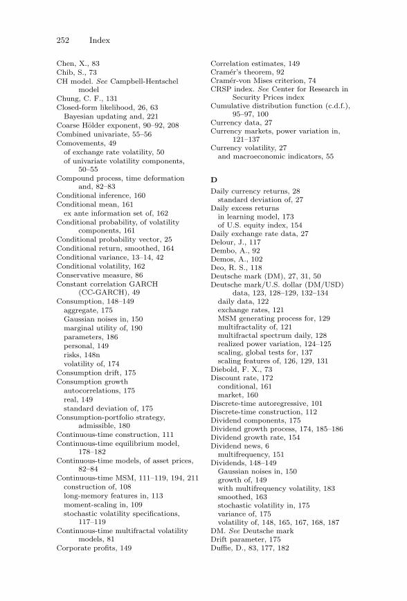
252 Index

Chen, X., 83Chib, S., 73CH model. See Campbell-Hentschel

modelChung, C. F., 131Closed-form likelihood, 26, 63

Bayesian updating and, 221Coarse Holder exponent, 90–92, 208Combined univariate, 55–56Comovements, 49

of exchange rate volatility, 50of univariate volatility components,

50–55Compound process, time deformation

and, 82–83Conditional inference, 160Conditional mean, 161

ex ante information set of, 162Conditional probability, of volatility

components, 161Conditional probability vector, 25Conditional return, smoothed, 164Conditional variance, 13–14, 42Conditional volatility, 162Conservative measure, 86Constant correlation GARCH

(CC-GARCH), 49Consumption, 148–149

aggregate, 175Gaussian noises in, 150marginal utility of, 190parameters, 186personal, 149risks, 148nvolatility of, 174

Consumption drift, 175Consumption growth

autocorrelations, 175real, 149standard deviation of, 175

Consumption-portfolio strategy,admissible, 180

Continuous-time construction, 111Continuous-time equilibrium model,

178–182Continuous-time models, of asset prices,

82–84Continuous-time MSM, 111–119, 194, 211

construction of, 108long-memory features in, 113moment-scaling in, 109stochastic volatility specifications,

117–119Continuous-time multifractal volatility

models, 81Corporate profits, 149

Correlation estimates, 149Cramer’s theorem, 92Cramer-von Mises criterion, 74CRSP index. See Center for Research in

Security Prices indexCumulative distribution function (c.d.f.),

95–97, 100Currency data, 27Currency markets, power variation in,

121–137Currency volatility, 27

and macroeconomic indicators, 55

D

Daily currency returns, 28standard deviation of, 27

Daily excess returnsin learning model, 173of U.S. equity index, 154

Daily exchange rate data, 27Delour, J., 117Dembo, A., 92Demos, A., 102Deo, R. S., 118Deutsche mark (DM), 27, 31, 50Deutsche mark/U.S. dollar (DM/USD)

data, 123, 128–129, 132–134daily data, 122exchange rates, 121MSM generating process for, 129multifractality of, 121multifractal spectrum daily, 128realized power variation, 124–125scaling, global tests for, 137scaling features of, 126, 129, 131

Diebold, F. X., 73Discount rate, 172

conditional, 161market, 160

Discrete-time autoregressive, 101Discrete-time construction, 112Dividend components, 175Dividend growth process, 174, 185–186Dividend growth rate, 154Dividend news, 6

multifrequency, 151Dividends, 148–149

Gaussian noises in, 150growth of, 149with multifrequency volatility, 183smoothed, 163stochastic volatility in, 175variance of, 175volatility of, 148, 165, 167, 168, 187

DM. See Deutsche markDrift parameter, 175Duffie, D., 83, 177, 182

Index 253

E

Economic intuition, 21, 60, 78, 161, 211Economic parameters, alternative

calibrations of, 164–165EIS. See Elasticity of intertemporal

substitutionElasticity of intertemporal substitution

(EIS), 148–150, 172Elerian, O., 73Embrechts, P., 84Engle, R. F., 2, 15Epstein, L., 148, 177, 220Epstein-Zin-Weil utility, 168n, 189Equilibrium dynamics, under isoelastic

utility, 181–182Equilibrium likelihood function, 158Equilibrium model

continuous-time, 178–182with endogenous price jumps, 178–182

Equilibrium price-dividend ratio,150, 187, 188

decrease in, 152numerical computation of, 150

Equilibrium stock prices, 181convergence of, 188multifrequency jump-diffusion, 183–185

Equity markets, 3, 58power variation in, 137–138

Equity premiumaverage, 154, 155effect of lower, 164increase of, 175magnitude of, 172

Equity returnsex post decomposition of, 162skewness of, 6, 8

Excess return. See also Daily excessreturns

determined, 168simulating single long sample of, 169

Excess return data, 153–154Excess return moments, 154Exchange economy, 148, 178Exchange rates

correlation of, 59DM/USD, 121

Expectation maximization (EM)algorithm, 26

Ex post decomposition, 222–223

F

Factor MSM, 205–207inference in, 206

Fama, E., 154FBM. See Fractional Brownian motionFederal Reserve Bank, 27Fed-treasury accord, 153

FIGARCH. See Fractionally integratedGARCH

Filtered probability, 160, 161Financial assets

demand for, 147log-price of, 82log return of, 13

Financial equilibrium, 179–182Financial leverage channel, 3Financial markets, 1, 179–182Financial returns

empirical properties of, 1–3unconditional distribution of, 3

First-order Markov vector, 20, 149,150, 168

Fisher, A. J., 26, 98, 103, 116, 117,121, 139, 218

Fractal dimension, 207Fractional Brownian motion (FBM),

84, 97in multifractal time, 101

Fractionally integrated GARCH(FIGARCH), 121, 131

estimation by maximum likelihood, 44partition function, 131vs. GARCH, 131–135vs. MSM, 42–46

Fractionally integrated processes, 23French, K., 154Frisch, U., 91Fully informed investors, empirical results

with, 153–165

G

Galluccio, S., 102GARCH. See Generalized autoregressive

conditional heteroskedasticityGaussian density, 25Gaussian process, 115, 116Geman, H., 177Generalized autoregressive conditional

heteroskedasticity (GARCH),5, 6, 13–15, 14n, 121

BIC test of, 35nmaximum likelihood estimation of,

35, 36–37multivariate, 16one-day forecasts, 39–40partition function, 131simulations, 130twenty-day forecasts, 41vs. FIGARCH, 131–135vs. MSM, 34–42

Generalized method of moments (GMM),66, 203

General motors (GM), 137–138Geometric progression, 106Ghashghaie, S., 102GM. See General motors

254 Index

GMM. See Generalized method ofmoments

Goodness of fit, 40Gordon growth formula, 164Granger, C. W. J., 24Gray, S., 4, 35Guivarc’h, Y., 88Gunther, T. A., 73

H

HAC. See Heteroskedasticity andautocorrelation consistent

HAC-adjusted Vuong test, 200–201Hadamard product, 25Halsey, T. C., 91Hamilton, J. D., 4, 8, 16, 17, 195Hansen, L. P., 152Harrison, J. M., 95, 98Hentschel, L., 6, 150, 158Heteroskedasticity and autocorrelation

consistent (HAC), 32, 38, 159nHigh-frequency components, 151, 185High-frequency multipliers, 151High-frequency volatility shocks, 3, 158Hill, B. M., 31Holder’s inequality, 96, 111, 209, 220Huang, C., 182Hull, J., 195, 226Hurvich, C. M., 118

I

Income flow, 147, 178–179Inference, 63–66

based on particle filter, 63–64in factor MSM, 206–207in multivariate MSM, 206–207

Interest rate, 149, 152, 172, 180, 184International Monetary Fund, 55Investor information, 168–169

full, 173intermediate, 173poor, 173

Investors, 171, 172, 178Isoelastic utility, 148

equilibrium dynamics under, 181–182

J

Jagannathan, R., 152Japanese yen (JA), 27, 31, 50Joint movements, 49Jump-diffusion, with countably many

frequencies, 187Jump processes, 83n

K

Khatchatrian, V., 174Klaassen, F., 34

Kolmogorov, A. N., 84Kozhemyak, A., 117, 220Kraft, D., 16Kreps, D., 95, 98Kurtosis, 158

calculating, 164of daily returns in learning model, 171endogenous, 165–172fall of, 170, 172, 173

L

Largest duration in yearly units (LDY),statistics of, 158

LDY. See Largest duration in yearly unitsLearning economy, 173, 223Learning model, 169–172

moments of, 170Ledoit, O., 207LeRoy, S., 169Lettau, M., 147, 148, 158Levy law, 102nLikelihood function, 63, 154. See also

Closed-form likelihoodequilibrium, 158optimized value of, 167simulated, 64

Likelihood ratio (LR), 55, 71Limiting MRW process, 219Limiting time deformation, 107–111Linearity property, 169Liquidity shocks, 2LMSV models. See Long-memory

stochastic volatility modelsLocal Holder exponent, 90–91, 194, 211Local Whittle estimator, 46Lockheed Martin, 137, 139Log consumption, 148Log-likelihood difference, 32, 34, 44Log-likelihood function, 26, 32Loglinear approximation, 172Loglinearized economy, 221Log-price

of financial assets, 82time-deformed, 97

Log-price process, 96convergence to, 187

Log volatility, 115, 116, 118autocovariogram of, 116, 219

Long-memory process, 15, 15n, 23–24, 99in non-Markovion regime switching

environment, 25nvolatility in, 99–100

Long-memory stochastic volatility(LMSV) models, 118

Long-run consumption risk, 148n, 152regime-switching formulation of, 175

Long-run price-dividend ratio, 172Low-frequency multipliers, 151, 185

Index 255

LR. See Likelihood ratioLu, Y., 118Lucas, R., 6, 145, 147, 194Lucas tree economy, 183, 185, 187, 188Ludvigson, S., 147, 158Lundblad, C., 174Lux, T., 99, 139, 140, 194

M

MAC method. See Memoryautocorrelation consistent method

Macroeconomic indicators, currencyvolatility and, 55

Madan, D., 177Maejima, M., 84Maheswaran, S., 101nMandelbrot, B. B., 15, 84, 85, 98, 117, 121Mantegna, R., 102Markov chain, 4, 16, 22, 25, 63, 64,

176, 193Markov process, 149, 150, 178, 181Markov state vector, 20, 25, 106, 183, 193Markov-switching GARCH

(MS-GARCH), 34maximum likelihood estimation of,

35, 36–37one-day forecasts, 39–40twenty-day forecasts, 41vs. MSM, 34–42

Markov-switching models, 16–17likelihood-based estimation of, 16n

Markov-switching multifractal (MSM),4, 8, 21, 105, 131

autocovariogram of log volatility in, 219binomial, 151bivariate. See Bivariate MSMcharacteristic of, 119in continuous-time. See

Continuous-time MSMwith countably many components,

107–114daily returns from, 5decomposition, 58with dependent arrivals, 114–115,

218–219in discrete time, 19–47, 112–114distribution of returns in, 32factor, 205–207failure rates, 76filtered version of symmetric, 164with finitely many components,

106–107forecasting across multiple horizons,

43–44generating process, for DM/USD

data, 129in-sample comparison, 35, 38long-run risk, 194

low-frequency components and longmemory with, 23–25

martingale version of, 131model selection, 32–34multivariate, 204–207multivariate extensions, 225–227one-day forecasts, 39out-of-sample forecasts, 35, 39parameters, 153partition functions, 131properties of, 5, 22–23sample paths, variations of, 110–111simulated log-returns of, 23of stochastic volatility, 20–25structure of, 195twenty-day forecasts, 41univariate, 60value-at-risk, 204volatility parameters, ML estimation

for, 155for volatility specification, 151vs. alternative specifications, 129–135vs. FIGARCH, 42–46vs. GARCH, 34–42vs. Markov-switching GARCH, 34–42

Markov-Switching Multifractal (MSM)equilibrium, 6, 159, 159n

free parameters of, 159full-information, 160, 161, 163volatility parameters of, 164

Markov-switching processes, 8Martingale property, 98Maximum likelihood (ML) estimation,

22, 25–26, 154–158bivariate MSM, 67in closed-form, 26combined calibration/estimation of,

155–157of GARCH, 35, 36–37of MS-GARCH, 35, 36–37results for currencies, 27, 28–32updating state vector, 25–26

McCracken, M., 38MCMC. See Monte Carlo Markov chainMean price-dividend ratio, 152Mean squared error (MSE), 40, 40n, 44Medium-run components, 151Memory autocorrelation consistent

(MAC) method, 46Merton, R. C., 82Mikkelsen, H. O., 42, 44, 131Mincer–Zarnowitz regressions, 35, 35n, 40MMAR. See Multifractal model of asset

returnsMoment-scaling, in continuous-time

MSM, 109Monte Carlo Markov chain (MCMC), 119Monte Carlo study, 139, 140nMonte Carlo tests, 103

256 Index

Motorola, 137, 139MRW. See Multifractal random walkMSE. See Mean squared errorMS-GARCH. See Markov-switching

GARCHMSM. See Markov-switching multifractalMuller, U., 102Multifractal deformation approach, 95Multifractal diffusions, 7, 89, 95, 97, 194Multifractality of price process, 97Multifractal jump-diffusion, 7, 177, 194

convergence to, 188Multifractal literature, 7–8, 115–117Multifractal measures, 81, 84, 89

binomial measure, 85–86multifractal spectrum of, 93random multiplicative cascades, 86–89

Multifractal model, 95, 101, 193with autocorrelated returns, 101–102

Multifractal model of asset returns(MMAR), 7, 95, 98–101, 115

development of, 102drawback of, 103features of, 99long memory in volatility, 99–100properties of, 98–101sample paths, 100–101unconditional distribution of returns,

98–99Multifractal price diffusion, 110–111Multifractal price process, 103Multifractal process, 95–96Multifractal random walk (MRW),

115–117Multifractal spectrum

of daily DM/USD data, 128local scales and, 89–91of multifractal measures, 93of price process, 100scaling function, 92

Multifractal time, Brownian motionin, 101

Multifractal time deformation, 95–98Multifractal trading time, 96Multifrequency consumption risk,

224–225preference implication and extension

to, 172Multifrequency economy, 183–184Multifrequency equilibrium model, 153Multifrequency jump-diffusions, 177–191

for equilibrium stock prices, 183–185Multifrequency risk

equilibrium implications of, 7pricing of, 6–7

Multifrequency shocks, 3on asset prices, 194

Multifrequency stochastic volatilitymodel, 19

Multifrequency volatility, 2, 24dividends with, 183modeling, 4–5

Multiplicative measures, spectrum of, 91Multistep forecasting, 4Multivariate GARCH, 16Multivariate MSM, 184, 204–205, 225

inference in, 206Muzy, J.-F., 116, 117, 139, 220

N

Newey, W., 38, 70, 77, 201, 203Nicolato, E., 119NYSE-AMEX-NASDAQ index, 137

O

Ordinary least squares (OLS), 127Ornstein-Uhlenbeck (O-U) processes,

118–119

P

Pagan, A., 153Pan, J., 83Paretian distributions, 22Parisi, G., 91Particle filter, 202–203

evaluation, 65inference based on, 63–64

Poisson process, 105Porter, R., 169Postwar data, 161–163Postwar sample, 155, 158–160

MSM specifications, 160Power variation

additional moments, 137–138in currency markets, 121–137data, 121–123in equity markets, 137–138global tests of fit, 136–137main empirical results, 123–129methodology, 123realized. See Realized power variation

Preference parameters, 172, 186Preferences, 148–149, 178–179Price differences, properties of, 102nPrice dividend ratio, 148n

average, 153. 154calibrated values of, 153computed, 168as deterministic function of

Markov state, 181discontinuous changes in, 181endogenous jumps in, 185equilibrium, 150, 187first-order expansion, 185increasing, 164loglinearizing, 184

Index 257

reduction of, 184risk premium of average, 175variance of, 169

Price jumps, 189–191application of, 190equilibrium model with endogenous,

178–182Price process, 95, 103, 187, 189

equilibrium, 188, 189log, 187multifractality of, 97stock, 180

Pricing dynamicswith an infinity of frequencies, 185endogenous multifrequency, 185–189

Pricing model, multifrequencyjumps in, 185

Probability integral transforms, 74Public equity, 179n

R

Random multiplicative cascades, 86–89Random walk, 148Realized monthly stock volatility (RV), 58Realized power variation

for CRSP index and GM, 138DM/USD, 124–125estimated slopes, 132–133FIGARCH simulations, 130GARCH simulations, 130MSM simulations, 130in scaling region for moments, 125for set of time scales and moments, 124sum of squared errors, 134–135

Recursive utility, 189–191Regime-switching models, 4, 22, 174

application of, 16estimation and forecasting methods for,

17Relative risk aversion, 172

coefficient of, 148, 152, 175, 180, 189Return decomposition, 162–164Return dynamics, equilibrium

price and, 186Return volatility, 165, 175Risk-free rate

annual, 155calibrated values of, 153proxied, 154

Rivers, D., 32Robinson, P. M., 15, 24, 46Rosenblatt, M., 73

S

Samorodnitsky, G., 84Santa-Clara, P., 207Scaling function, 92, 209Scholes, M., 82

Schwert, G. W., 153, 154SDF. See Stochastic discount factorSelf-similar process, 81, 83, 96Shephard, N., 73, 118, 119Shiller, R., 169Short memory processes, 15Sims, C., 101nSimulated likelihood, 64Singleton, K., 83Skewness, 164

of daily returns in learning model, 171increase of, 172negative, 158, 165, 170, 173

Smoothed probability, 160, 161, 222–223Sørensen, B., 140Sornette, D., 139SSE. See Sum of squared errorsStandard Brownian motion, 100Standard deviation

of consumption growth, 175of daily currency returns, 27of U.S. real dividend growth, 153–154,

155n, 183Stanley, H. E., 102Stochastic discount factor (SDF), 149,

168, 220price jumps in, 190

Stochastic process, 7, 82, 95–96,177–178, 200

Stochastic time deformation, 96Stochastic volatility, 31, 183

correlated, 184in dividends, 175long-memory, 15MSM model of, 20–25

Stochastic volatility (SV) models, 14,19, 22, 110, 118

Stochastic volatility literature, 14nStochastic volatility specifications,

117–119Stock, 137, 179, 183Stock market, 148Stock prices, 153, 180

change of, 182decrease of aggregate, 148equilibrium. See Equilibrium stock

pricesStock returns, 3, 7, 149, 168–169

conditional mean of, 160, 162equilibrium, 152–153gross, 150log excess, 150, 152, 153variance of, 160, 162, 175

Student distribution, 35Sum of squared errors (SSE), 131,

140n, 141nSV models. See Stochastic volatility

models

258 Index

T

Tail behavior, 95, 97, 98, 100Tail index, 31, 31nTail risk, 2Taqqu, M. S., 84Tata, F., 102Tay, S. A., 73Thompson, S. B., 117Tieslau, M. A., 131Time deformation, 81, 95, 98, 103

and compound process, 82–83multifractal, 96–98, 103stochastic, 96

Time-deformed Brownian motions, 97Time-deformed log-price, 97Trading time, 98, 110, 210Transition matrix, 63Two-asset economy, 98Two-state Lucas economy, drift in, 147

U

Uncertainty channel, 169Unifractal, 96Uniscaling, 96United Airlines (UAL), 137, 139U.S. dollar, 27

V

Value-at-risk (VaR), 75van der Vaart, A. W., 92van Ness, J. W., 15Vassilicos, J. C., 102Venardos, E., 119Veronesi, P., 7, 147, 176Volatility

arrival vector, 60comovements in, 49conditional distribution of, 160, 162dividends, 148, 165, 167, 187ergodic distribution of, 62of excess returns, 158feedback effect of, 165, 185, 186increase and decrease of, 171joint movements in, 49long memory in, 99–100properties, 62state vector, 165stochastic specification, 60–62

Volatility clustering, 2Volatility components, 49, 158, 193

comovements univariate of, 50–55conditional probabilities of, 161construction of, 61consumption of, 168correlated, 53, 174dividends of, 168ergodic distribution of, 201–202exchange rates, 50in high state, 160, 161magnitude of, 152mark and yen series, 55noisy observations of, 168varying, 154, 155

Volatility feedback, 154–158dividend, 175estimated, 165increase of, 158, 175with multifrequency shocks, 151–153robustness of, 170, 172smoothed, 163unconditional, 158

Volatility forecasting, 2Volatility shocks, 4, 15

half-life of, 159highest-frequency, 3, 158lowest-frequency, 158persistent, 165

Vuong, Q., 32, 35, 71, 72, 155, 159

W

Wachter, J., 147, 158Weil, P., 148, 177West, K., 38, 70, 77, 201, 203Whaley, R., 4White, A., 195, 226Wolf, M., 207Wooldridge, J., 16

Y

Yaron, A., 6, 147–149, 174, 175, 195Yor, M., 177

Z

Zame, W., 182Zeitouni, O., 92Zin, S., 148, 177, 220