Embed Size (px)
Citation preview
TDB − NLA Parallel Algorithms for Scientific Computing
Multigrid methods
Algebraic Multigrid methodsAlgebraic Multilevel Iteration
methods
– p. 1/25
Residual correction
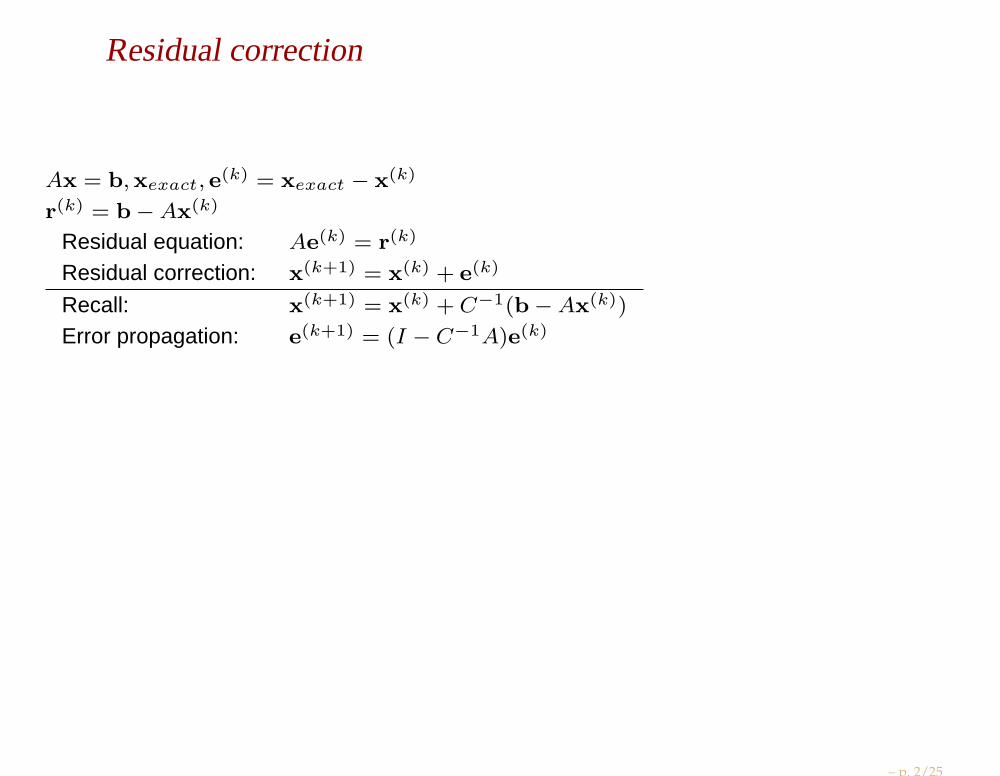
Ax = b,xexact, e(k) = xexact − x(k)
r(k) = b−Ax(k)
Residual equation: Ae(k) = r(k)
Residual correction: x(k+1) = x(k) + e(k)
Recall: x(k+1) = x(k) + C−1(b−Ax(k))
Error propagation: e(k+1) = (I − C−1A)e(k)
– p. 2/25
TDB − NLA Parallel Algorithms for Scientific Computing
Run Jacobi demo...
student/NLA/Demos/Module3/L5
– p. 3/25
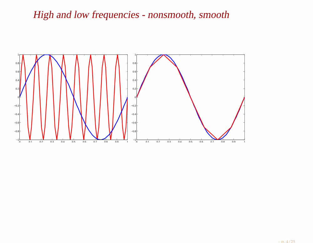
High and low frequencies - nonsmooth, smooth
0 0.1 0.2 0.3 0.4 0.5 0.6 0.7 0.8 0.9 1−1
−0.8
−0.6
−0.4
−0.2
0
0.2
0.4
0.6
0.8
1
0 0.1 0.2 0.3 0.4 0.5 0.6 0.7 0.8 0.9 1−1
−0.8
−0.6
−0.4
−0.2
0
0.2
0.4
0.6
0.8
1
– p. 4/25
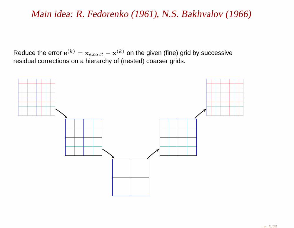
Main idea: R. Fedorenko (1961), N.S. Bakhvalov (1966)
Reduce the error e(k) = xexact − x(k) on the given (fine) grid by successiveresidual corrections on a hierarchy of (nested) coarser grids.
– p. 5/25
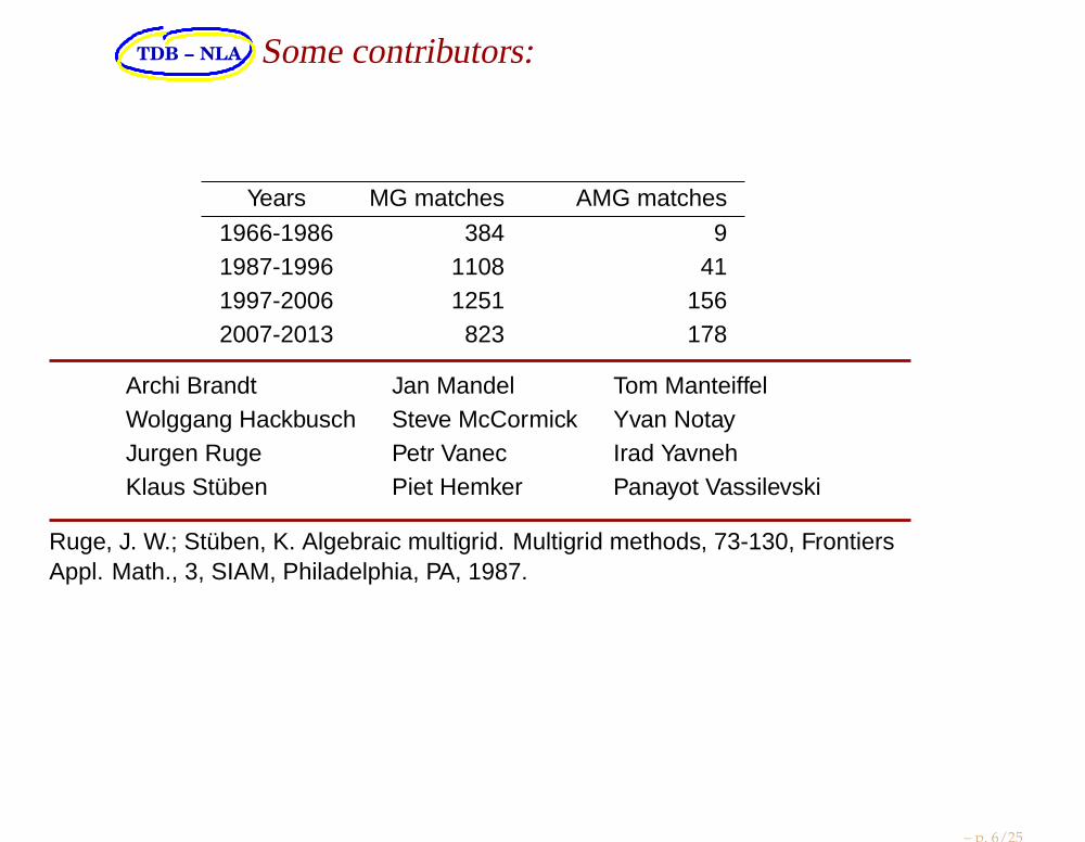
TDB − NLA Some contributors:
Years MG matches AMG matches
1966-1986 384 91987-1996 1108 411997-2006 1251 1562007-2013 823 178
Archi Brandt Jan Mandel Tom ManteiffelWolggang Hackbusch Steve McCormick Yvan NotayJurgen Ruge Petr Vanec Irad YavnehKlaus Stüben Piet Hemker Panayot Vassilevski
Ruge, J. W.; Stüben, K. Algebraic multigrid. Multigrid methods, 73-130, FrontiersAppl. Math., 3, SIAM, Philadelphia, PA, 1987.
– p. 6/25
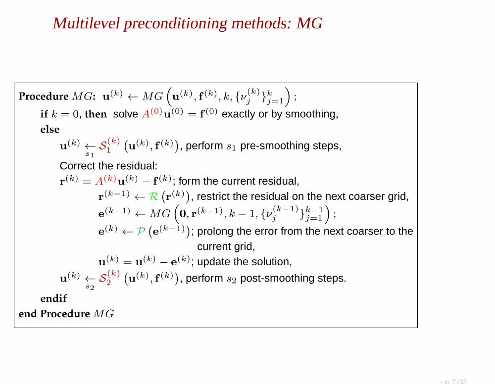
Multilevel preconditioning methods: MG
Procedure MG: u(k) ←MG(u(k), f (k), k, ν
(k)j
kj=1
);
if k = 0, then solve A(0)u(0) = f (0) exactly or by smoothing,else
u(k) ←s1S(k)1
(u(k), f (k)
), perform s1 pre-smoothing steps,
Correct the residual:r(k) = A(k)u(k) − f (k); form the current residual,
r(k−1) ← R(r(k)
), restrict the residual on the next coarser grid,
e(k−1) ←MG(0, r(k−1), k − 1, ν
(k−1)j k−1
j=1
);
e(k) ← P(e(k−1)
); prolong the error from the next coarser to the
current grid,u(k) = u(k) − e(k); update the solution,
u(k) ←s2S(k)2
(u(k), f (k)
), perform s2 post-smoothing steps.
endif
end Procedure MG
– p. 7/25
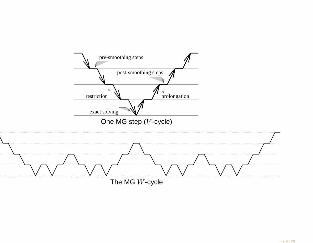
post-smoothing steps
pre-smoothing steps
exact solving
restriction prolongation
One MG step (V -cycle)
The MG W -cycle
– p. 8/25
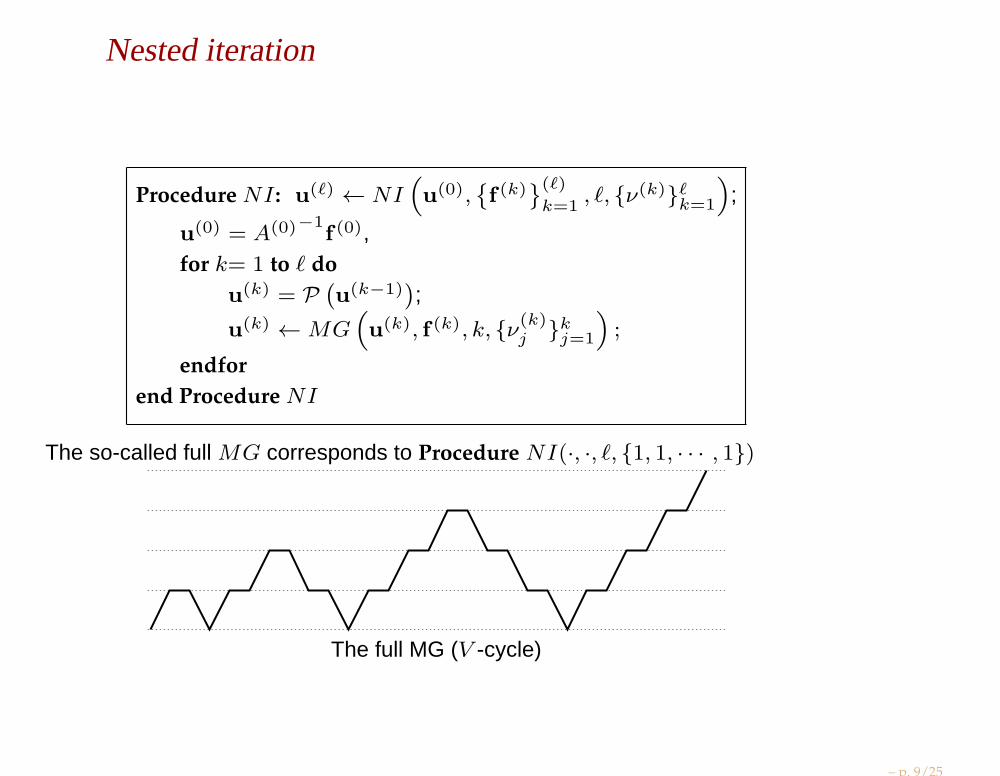
Nested iteration
Procedure NI : u(ℓ) ← NI(u(0),
f (k)
(ℓ)k=1
, ℓ, ν(k)ℓk=1
);
u(0) = A(0)−1f (0),
for k= 1 to ℓ do
u(k) = P(u(k−1)
);
u(k) ←MG(u(k), f (k), k, ν
(k)j
kj=1
);
endfor
end Procedure NI
The so-called full MG corresponds to Procedure NI(·, ·, ℓ, 1, 1, · · · , 1)
The full MG (V -cycle)
– p. 9/25
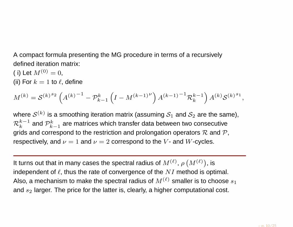
A compact formula presenting the MG procedure in terms of a recursivelydefined iteration matrix:( i) Let M(0) = 0,(ii) For k = 1 to ℓ, define
M(k) = S(k)s2(A(k)−1
− Pkk−1
(I −M(k−1)ν
)A(k−1)−1
Rk−1k
)A(k)S(k)
s1,
where S(k) is a smoothing iteration matrix (assuming S1 and S2 are the same),Rk−1
kand Pk
k−1 are matrices which transfer data between two consecutivegrids and correspond to the restriction and prolongation operators R and P ,respectively, and ν = 1 and ν = 2 correspond to the V - and W -cycles.
It turns out that in many cases the spectral radius of M(ℓ), ρ(M(ℓ)
), is
independent of ℓ, thus the rate of convergence of the NI method is optimal.Also, a mechanism to make the spectral radius of M(ℓ) smaller is to choose s1
and s2 larger. The price for the latter is, clearly, a higher computational cost.
– p. 10/25
MG ingredients
smoothers (many different)
Jacobi, weighted Jacobi (ωdiag(A), GS, SOR, SSOR, SPAI
restriction and prolongation operators
coarse level matrix (approximation properties)
– p. 11/25
47 of 119
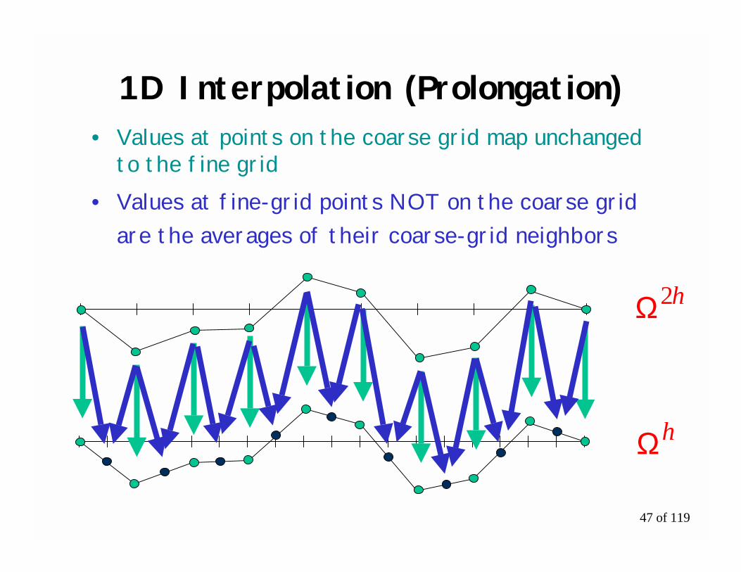
1D Interpolation (Prolongation)
Ωh
Ω2h
• Values at points on the coarse grid map unchangedto the fine grid
• Values at fine-grid points NOT on the coarse gridare the averages of their coarse-grid neighbors
52 of 119
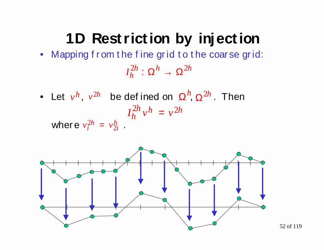
1D Restriction by injection• Mapping from the fine grid to the coarse grid:
• Let , be defined on , . Then
where .
vh v2h Ωh Ω2h
vv hi
hi 22 =
I hhhh
22 Ω→Ω:
vvI hhhh
22 =
53 of 119
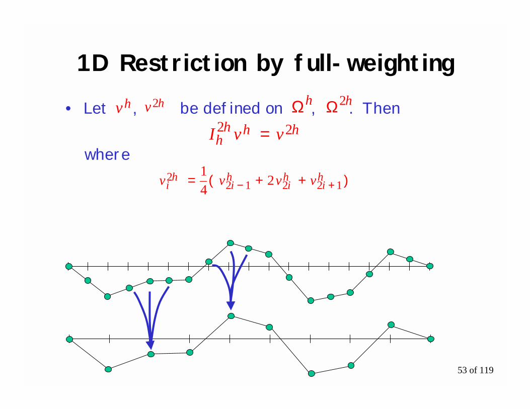
1D Restriction by full-weighting
• Let , be defined on , . Then
where
vh v2h Ωh Ω2h
vvvv hi
hi
hi
hi 122122 )++(= 2
41
+−
vvI hhhh
22 =
55 of 119
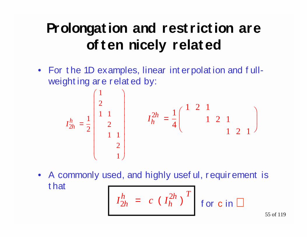
Prolongation and restriction areoften nicely related
• For the 1D examples, linear interpolation and full-weighting are related by:
• A commonly used, and highly useful, requirement isthat
for c in ℜIcI 22
Thh
hh )(=
I2hh
=
1211
211
21
21 I h
h2
=121
121121
41
56 of 119
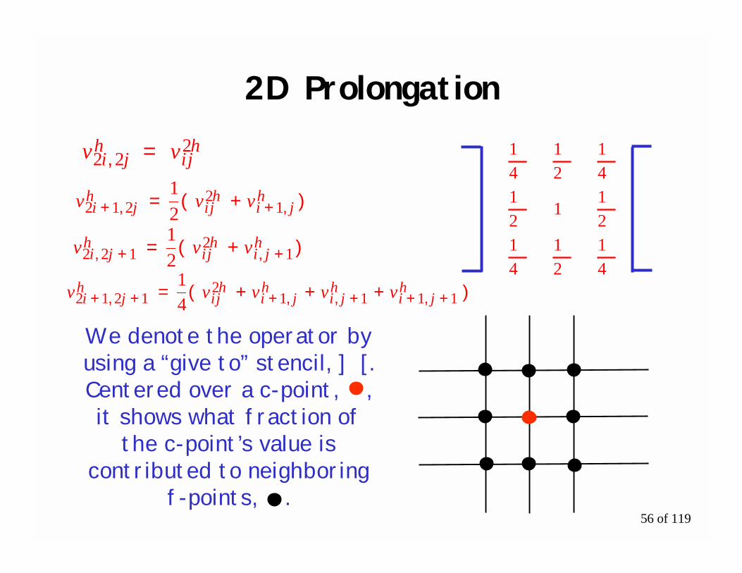
2D Prolongation
vv 222
hji
hji, =
vvv 12
212h
jihji
hji ,+,+ )+(=
21
vvv 12
122h
jihji
hji +,+, )+(=
21
vvvvv 11112
1212h
jih
jih
jihji
hji +,++,,++,+ )+++(=
41 4
121
41
21
121
41
21
41
We denote the operator byusing a “give to” stencil, ] [.Centered over a c-point, ,it shows what fraction of
the c-point’s value iscontributed to neighboring
f-points, .
57 of 119
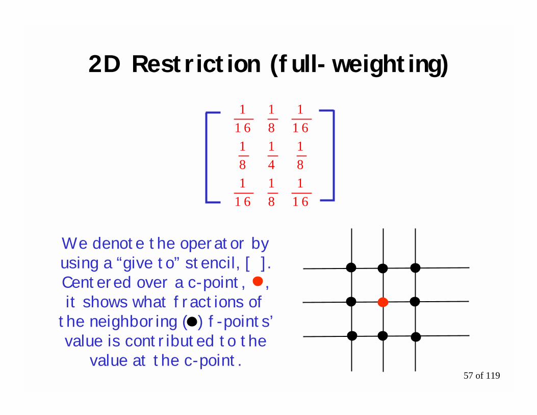
2D Restriction (full-weighting)
We denote the operator byusing a “give to” stencil, [ ].Centered over a c-point, ,it shows what fractions of
the neighboring ( ) f-points’value is contributed to the
value at the c-point.
611
81
611
81
41
81
611
81
611
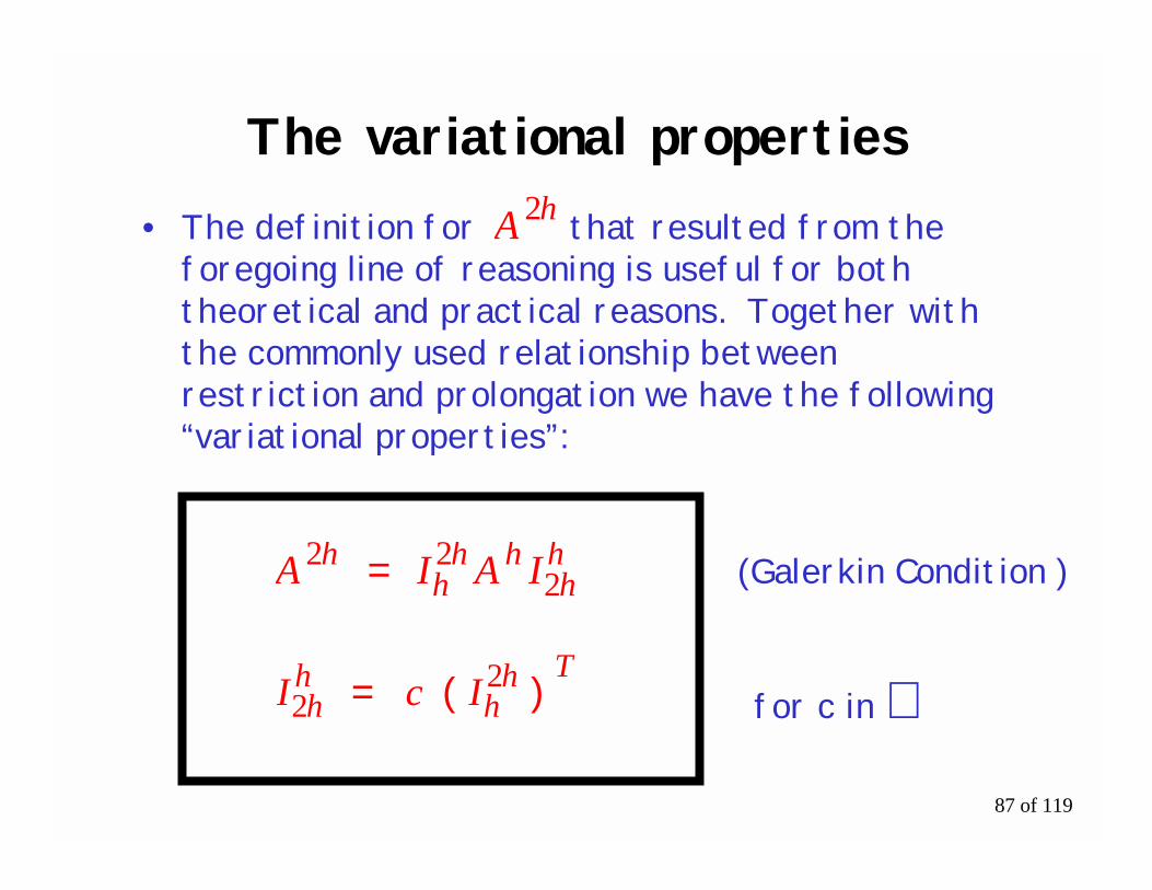
87 of 119
The variational properties• The definition for that resulted from the
foregoing line of reasoning is useful for boththeoretical and practical reasons. Together withthe commonly used relationship betweenrestriction and prolongation we have the following“variational properties”:
IAIA 222 h
hhh
hh =
IcI 22
Thh
hh )(=
(Galerkin Condition )
for c in ℜ
A 2h
MG: Rate of convergence and computational complexity
– p. 12/25
TDB − NLA Algebraic Multigrid
– p. 13/25
AMG demo ...AGMG http://homepages.ulb.ac.be/~ynotay/AGMG/
.../Projects/ComplexSymmetric
– p. 14/25
11
Lawrence Livermore National Laboratory
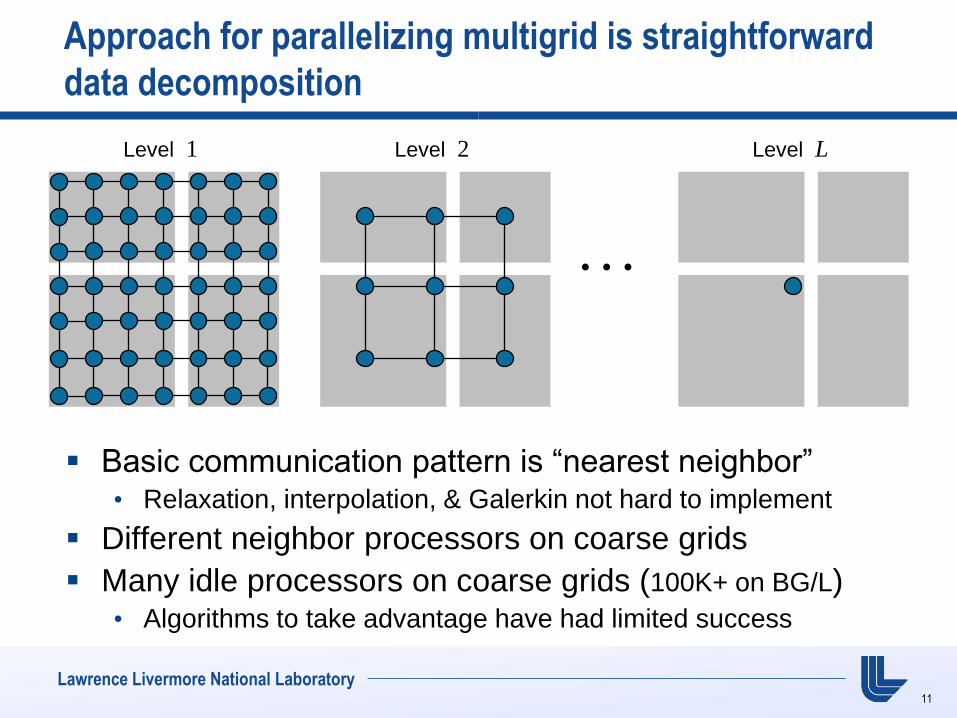
Approach for parallelizing multigrid is straightforward
data decomposition
Basic communication pattern is “nearest neighbor” • Relaxation, interpolation, & Galerkin not hard to implement
Different neighbor processors on coarse grids
Many idle processors on coarse grids (100K+ on BG/L) • Algorithms to take advantage have had limited success
Level 1
Level 2
Level L
12
Lawrence Livermore National Laboratory
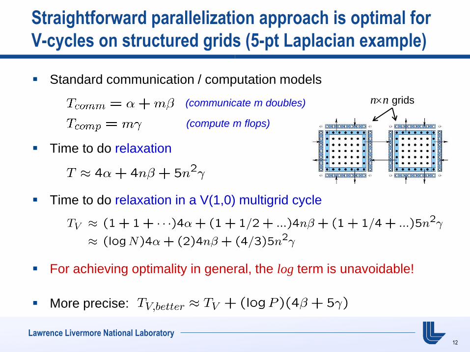
Straightforward parallelization approach is optimal for
V-cycles on structured grids (5-pt Laplacian example)
Standard communication / computation models
Time to do relaxation
Time to do relaxation in a V(1,0) multigrid cycle
For achieving optimality in general, the log term is unavoidable!
More precise:
(communicate m doubles)
(compute m flops)
nn grids
13
Lawrence Livermore National Laboratory
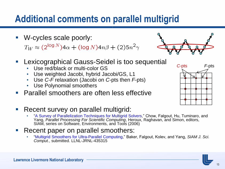
Additional comments on parallel multigrid
W-cycles scale poorly:
Lexicographical Gauss-Seidel is too sequential
• Use red/black or multi-color GS • Use weighted Jacobi, hybrid Jacobi/GS, L1 • Use C-F relaxation (Jacobi on C-pts then F-pts) • Use Polynomial smoothers
Parallel smoothers are often less effective
Recent survey on parallel multigrid: • “A Survey of Parallelization Techniques for Multigrid Solvers,” Chow, Falgout, Hu, Tuminaro, and
Yang, Parallel Processing For Scientific Computing, Heroux, Raghavan, and Simon, editors, SIAM, series on Software, Environments, and Tools (2006)
Recent paper on parallel smoothers: • “Multigrid Smoothers for Ultra-Parallel Computing,” Baker, Falgout, Kolev, and Yang, SIAM J. Sci.
Comput., submitted. LLNL-JRNL-435315
C-pts F-pts
14
Lawrence Livermore National Laboratory
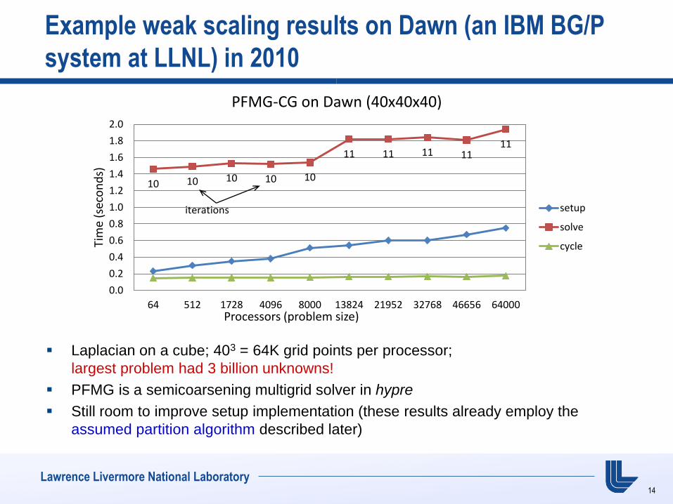
Example weak scaling results on Dawn (an IBM BG/P
system at LLNL) in 2010
Laplacian on a cube; 403 = 64K grid points per processor;
largest problem had 3 billion unknowns!
PFMG is a semicoarsening multigrid solver in hypre
Still room to improve setup implementation (these results already employ the
assumed partition algorithm described later)
10 10 10 10 10
11 11 11 11 11
0.0
0.2
0.4
0.6
0.8
1.0
1.2
1.4
1.6
1.8
2.0
64 512 1728 4096 8000 13824 21952 32768 46656 64000
Tim
e (s
eco
nd
s)
Processors (problem size)
PFMG-CG on Dawn (40x40x40)
setup
solve
cycle
iterations
15
Lawrence Livermore National Laboratory
Basic multigrid research challenge
Optimal O(N) multigrid methods don‟t exist for some applications, even in serial
Need to invent methods for these applications
However …
Some of the classical and most proven techniques used in multigrid methods don‟t parallelize • Gauss-Seidel smoothers are inherently sequential
• W-cycles have poor parallel scaling
Parallel computing imposes additional restrictions on multigrid algorithmic development
25
Lawrence Livermore National Laboratory
Choosing the coarse grid
In C-AMG, the coarse grid is a subset of the fine grid
The basic coarsening procedure is as follows:
• Define a strength matrix As by deleting weak connections in A
• First pass: Choose an independent set of fine-grid points based
on the graph of As
• Second pass: Choose additional points if needed to satisfy
interpolation requirements
Coarsening partitions the grid into C- and F-points
26
Lawrence Livermore National Laboratory
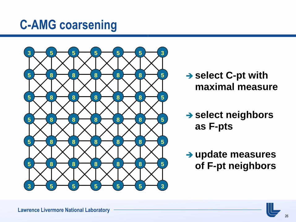
C-AMG coarsening
select C-pt with maximal measure
select neighbors as F-pts
update measures of F-pt neighbors
3 5 5 5 5 5 3
5 8 8 8 8 8 5
5 8 8 8 8 8 5
5 8 8 8 8 8 5
5 8 8 8 8 8 5
5 8 8 8 8 8 5
3 5 5 5 5 5 3
27
Lawrence Livermore National Laboratory
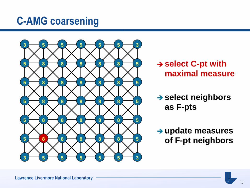
C-AMG coarsening
select C-pt with maximal measure
select neighbors as F-pts
update measures of F-pt neighbors
3 5 5 5 5 5 3
5 8 8 8 8 8 5
5 8 8 8 8 8 5
5 8 8 8 8 8 5
5 8 8 8 8 8 5
5 8 8 8 8 8 5
3 5 5 5 5 5 3
28
Lawrence Livermore National Laboratory
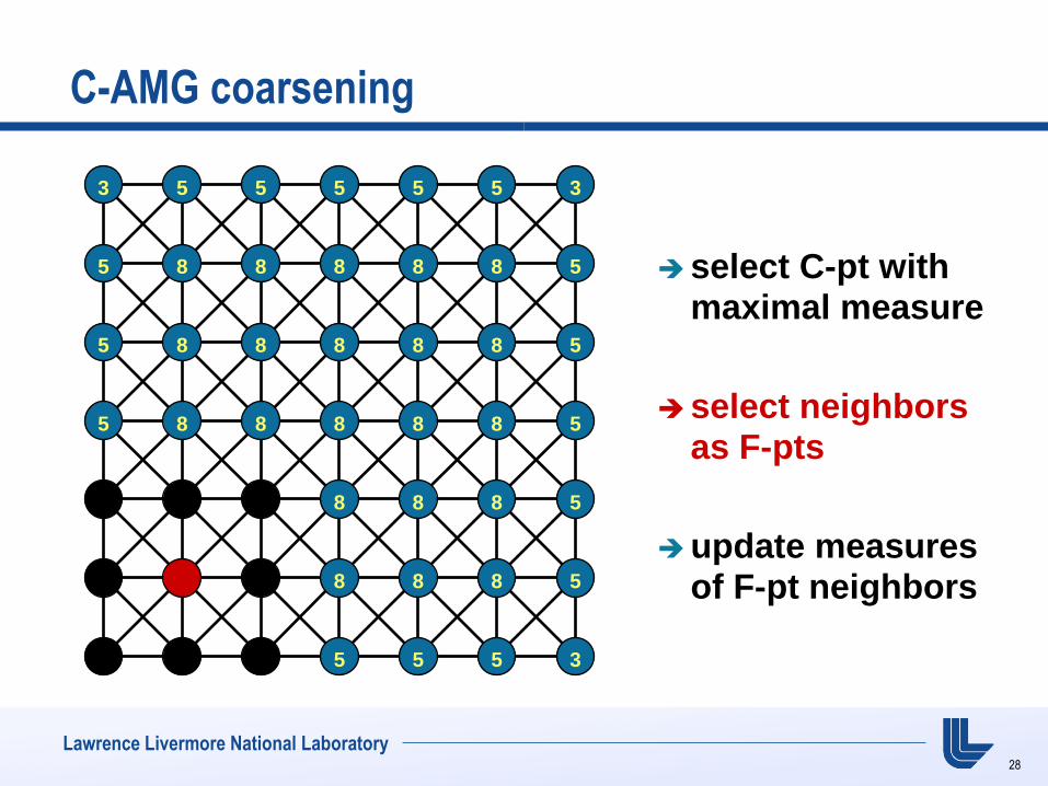
C-AMG coarsening
select C-pt with maximal measure
select neighbors as F-pts
update measures of F-pt neighbors
3 5 5 5 5 5 3
5 8 8 8 8 8 5
5 8 8 8 8 8 5
5 8 8 8 8 8 5
8 8 8 5
8 8 8 5
5 5 5 3
29
Lawrence Livermore National Laboratory
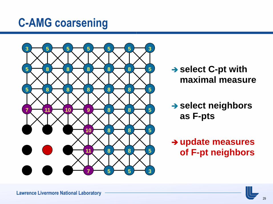
C-AMG coarsening
select C-pt with maximal measure
select neighbors as F-pts
update measures of F-pt neighbors
3 5 5 5 5 5 3
5 8 8 8 8 8 5
5 8 8 8 8 8 5
7 11 10 9 8 8 5
10 8 8 5
11 8 8 5
7 5 5 3
30
Lawrence Livermore National Laboratory
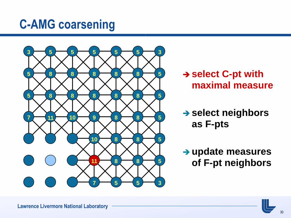
C-AMG coarsening
select C-pt with maximal measure
select neighbors as F-pts
update measures of F-pt neighbors
3 5 5 5 5 5 3
5 8 8 8 8 8 5
5 8 8 8 8 8 5
7 11 10 9 8 8 5
10 8 8 5
8 8 5
7 5 5 3
11
31
Lawrence Livermore National Laboratory
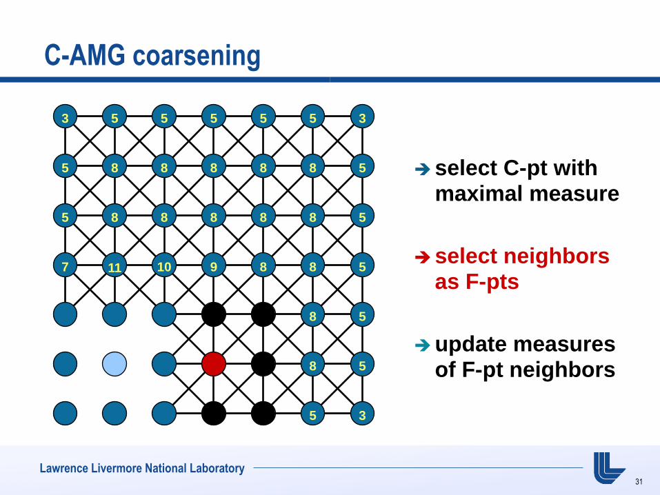
C-AMG coarsening
select C-pt with maximal measure
select neighbors as F-pts
update measures of F-pt neighbors
3 5 5 5 5 5 3
5 8 8 8 8 8 5
5 8 8 8 8 8 5
7 11 10 9 8 8 5
8 5
8 5
5 3
32
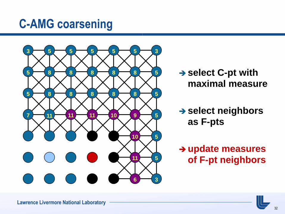
Lawrence Livermore National Laboratory
C-AMG coarsening
select C-pt with maximal measure
select neighbors as F-pts
update measures of F-pt neighbors
3 5 5 5 5 5 3
5 8 8 8 8 8 5
5 8 8 8 8 8 5
7 11 11 11 10 9 5
10 5
11 5
6 3
33
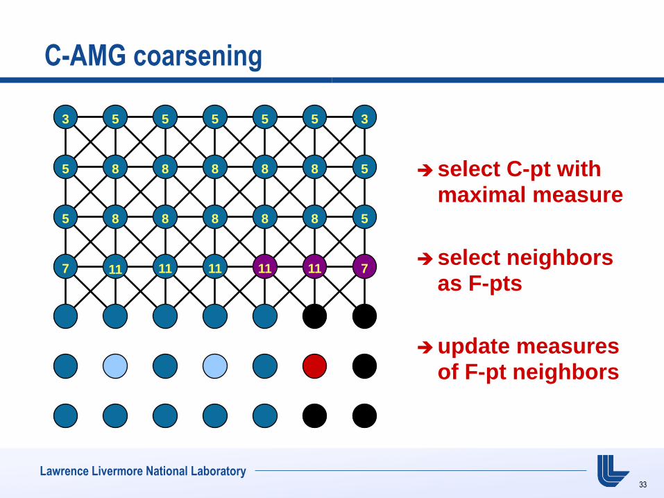
Lawrence Livermore National Laboratory
C-AMG coarsening
select C-pt with maximal measure
select neighbors as F-pts
update measures of F-pt neighbors
3 5 5 5 5 5 3
5 8 8 8 8 8 5
5 8 8 8 8 8 5
7 11 11 11 11 11 7
34
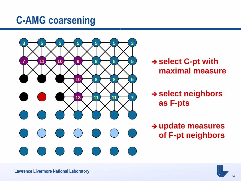
Lawrence Livermore National Laboratory
C-AMG coarsening
select C-pt with maximal measure
select neighbors as F-pts
update measures of F-pt neighbors
3 5 5 5 5 5 3
7 11 10 9 8 8 5
10 8 8 5
13 11 11 7
35
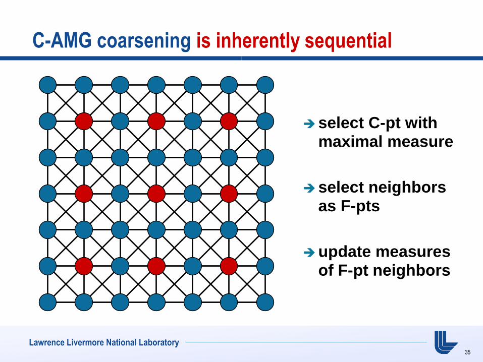
Lawrence Livermore National Laboratory
C-AMG coarsening is inherently sequential
select C-pt with maximal measure
select neighbors as F-pts
update measures of F-pt neighbors
44
Lawrence Livermore National Laboratory
Parallel Coarsening Algorithms
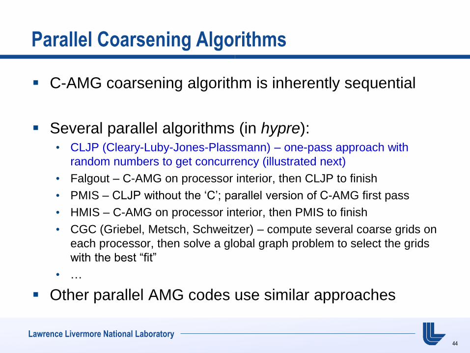
C-AMG coarsening algorithm is inherently sequential
Several parallel algorithms (in hypre): • CLJP (Cleary-Luby-Jones-Plassmann) – one-pass approach with
random numbers to get concurrency (illustrated next)
• Falgout – C-AMG on processor interior, then CLJP to finish
• PMIS – CLJP without the „C‟; parallel version of C-AMG first pass
• HMIS – C-AMG on processor interior, then PMIS to finish
• CGC (Griebel, Metsch, Schweitzer) – compute several coarse grids on
each processor, then solve a global graph problem to select the grids
with the best “fit”
• …
Other parallel AMG codes use similar approaches
45
Lawrence Livermore National Laboratory
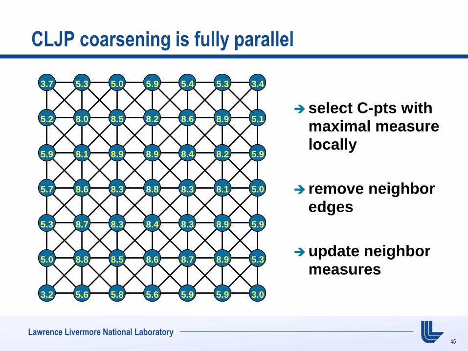
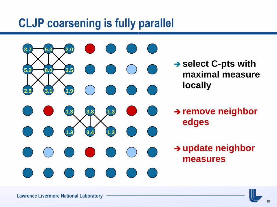
CLJP coarsening is fully parallel
select C-pts with maximal measure locally
remove neighbor edges
update neighbor measures
3.7 5.3 5.0 5.9 5.4 5.3 3.4
5.2 8.0 8.5 8.2 8.6 8.9 5.1
5.9 8.1 8.9 8.9 8.4 8.2 5.9
5.7 8.6 8.3 8.8 8.3 8.1 5.0
5.3 8.7 8.3 8.4 8.3 8.9 5.9
5.0 8.8 8.5 8.6 8.7 8.9 5.3
3.2 5.6 5.8 5.6 5.9 5.9 3.0

46
Lawrence Livermore National Laboratory
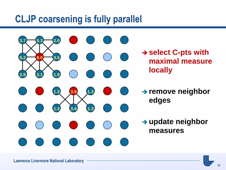
CLJP coarsening is fully parallel
select C-pts with maximal measure locally
remove neighbor edges
update neighbor measures
3.7 5.3 5.0 5.9 5.4 5.3 3.4
5.2 8.0 8.5 8.2 8.6 8.9 5.1
5.9 8.1 8.9 8.9 8.4 8.2 5.9
5.7 8.6 8.3 8.8 8.3 8.1 5.0
5.3 8.7 8.3 8.4 8.3 8.9 5.9
5.0 8.8 8.5 8.6 8.7 8.9 5.3
3.2 5.6 5.8 5.6 5.9 5.9 3.0
47
Lawrence Livermore National Laboratory
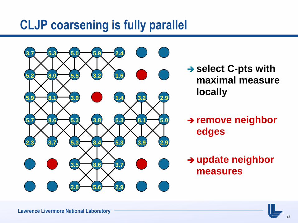
CLJP coarsening is fully parallel
select C-pts with maximal measure locally
remove neighbor edges
update neighbor measures
3.7 5.3 5.0 5.9 2.4
5.2 8.0 5.5 3.2 1.6
5.9 8.1 3.9 1.4 3.2 2.9
5.7 8.6 5.3 3.8 5.3 8.1 5.0
2.3 3.7 5.3 8.4 5.3 3.9 2.9
3.5 8.6 3.7
2.8 5.6 2.9
48
Lawrence Livermore National Laboratory
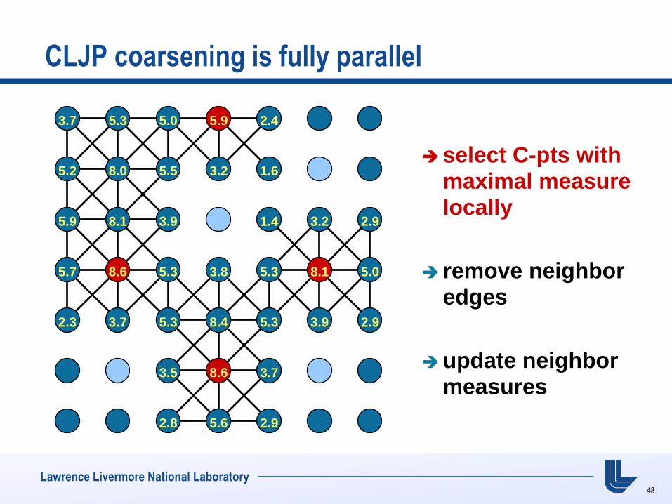
CLJP coarsening is fully parallel
select C-pts with maximal measure locally
remove neighbor edges
update neighbor measures
3.7 5.3 5.0 5.9 2.4
5.2 8.0 5.5 3.2 1.6
5.9 8.1 3.9 1.4 3.2 2.9
5.7 8.6 5.3 3.8 5.3 8.1 5.0
2.3 3.7 5.3 8.4 5.3 3.9 2.9
3.5 8.6 3.7
2.8 5.6 2.9
49
Lawrence Livermore National Laboratory
CLJP coarsening is fully parallel
select C-pts with maximal measure locally
remove neighbor edges
update neighbor measures
3.7 5.3 2.0
5.2 8.0 3.5
2.9 3.1 1.9
1.3 3.8 1.3
1.3 3.4 1.3
50
Lawrence Livermore National Laboratory
CLJP coarsening is fully parallel
select C-pts with maximal measure locally
remove neighbor edges
update neighbor measures
3.7 5.3 2.0
5.2 8.0 3.5
2.9 3.1 1.9
1.3 3.8 1.3
1.3 3.4 1.3
51
Lawrence Livermore National Laboratory
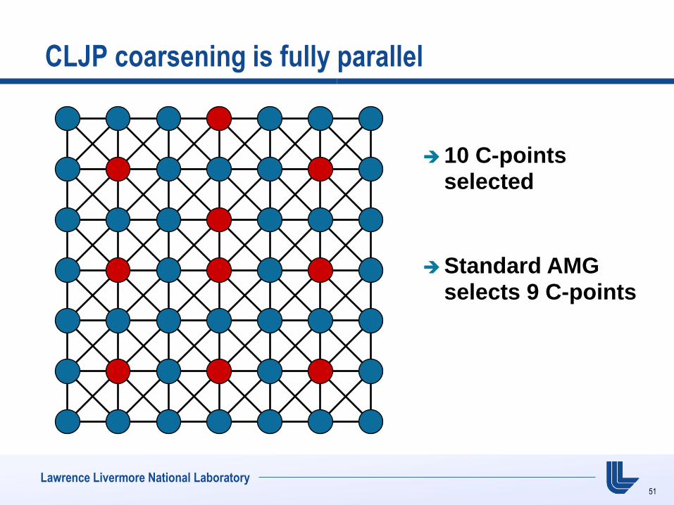
CLJP coarsening is fully parallel
10 C-points selected
Standard AMG selects 9 C-points
52
Lawrence Livermore National Laboratory
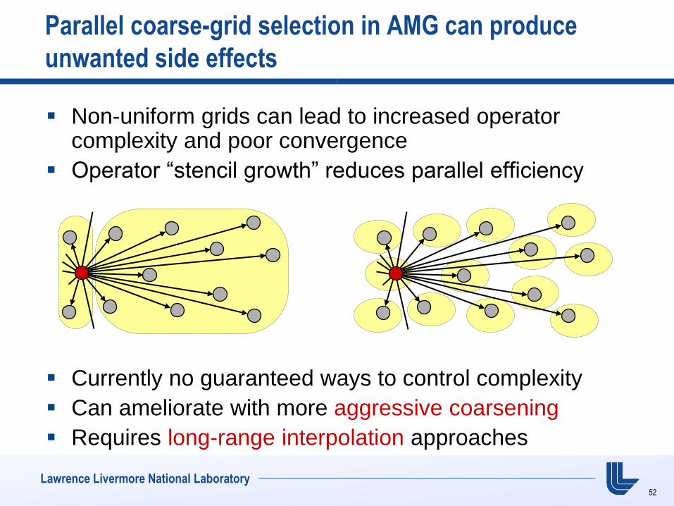
Parallel coarse-grid selection in AMG can produce
unwanted side effects
Non-uniform grids can lead to increased operator complexity and poor convergence
Operator “stencil growth” reduces parallel efficiency
Currently no guaranteed ways to control complexity
Can ameliorate with more aggressive coarsening
Requires long-range interpolation approaches
56
Lawrence Livermore National Laboratory
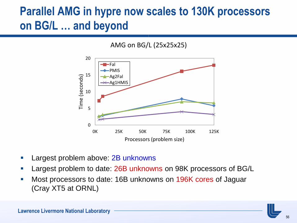
Parallel AMG in hypre now scales to 130K processors
on BG/L … and beyond
Largest problem above: 2B unknowns
Largest problem to date: 26B unknowns on 98K processors of BG/L
Most processors to date: 16B unknowns on 196K cores of Jaguar
(Cray XT5 at ORNL)
0
5
10
15
20
0K 25K 50K 75K 100K 125K
Tim
e (s
eco
nd
s)
Processors (problem size)
AMG on BG/L (25x25x25)
FalPMISAg2FalAg1HMIS
59
Lawrence Livermore National Laboratory
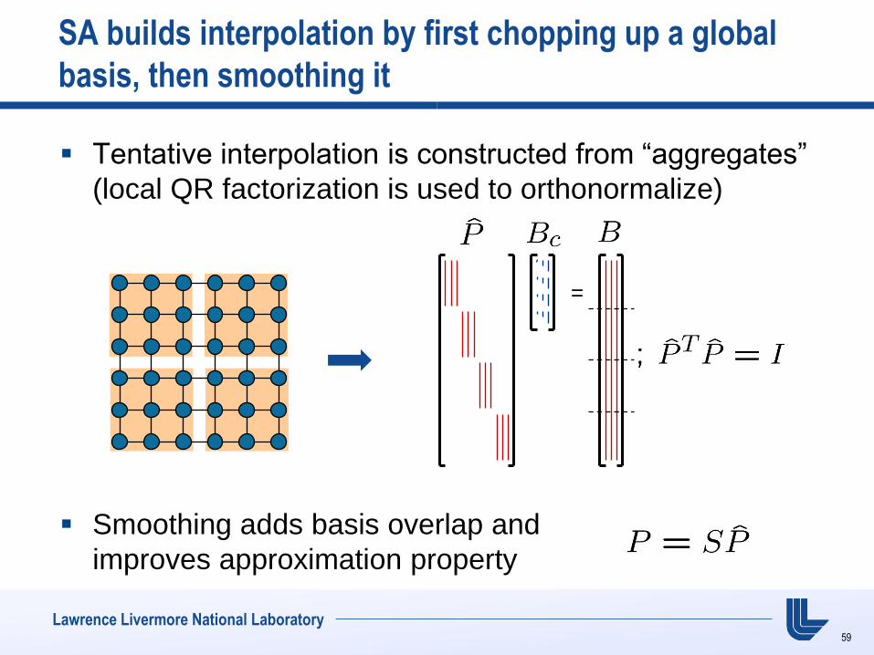
SA builds interpolation by first chopping up a global
basis, then smoothing it
Tentative interpolation is constructed from “aggregates”
(local QR factorization is used to orthonormalize)
Smoothing adds basis overlap and
improves approximation property
=
60
Lawrence Livermore National Laboratory
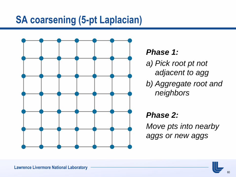
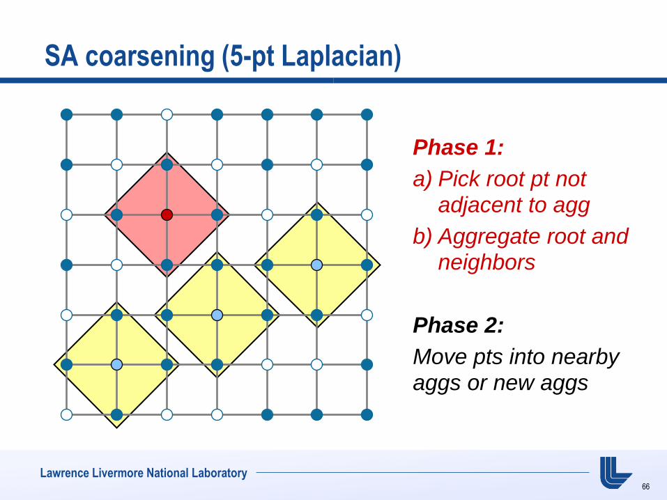
SA coarsening (5-pt Laplacian)
Phase 1:
a) Pick root pt not adjacent to agg
b) Aggregate root and neighbors
Phase 2:
Move pts into nearby
aggs or new aggs
61
Lawrence Livermore National Laboratory
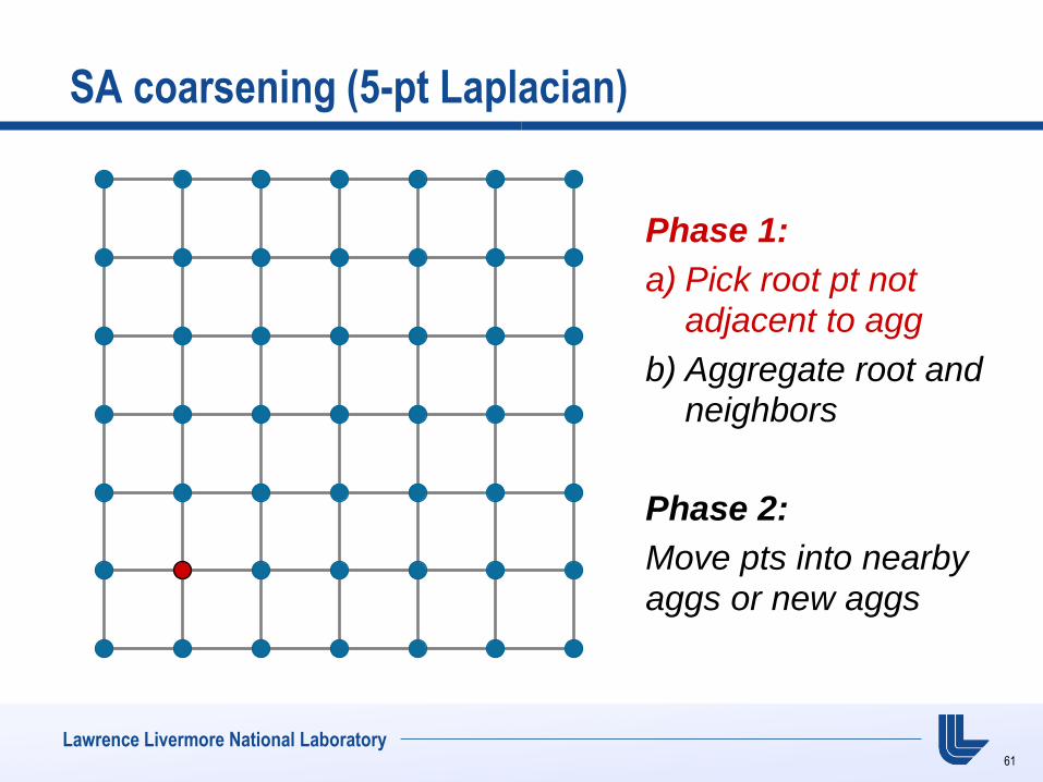
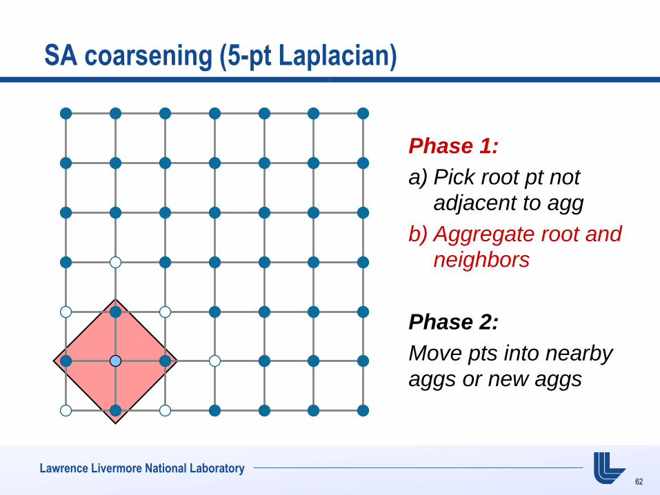
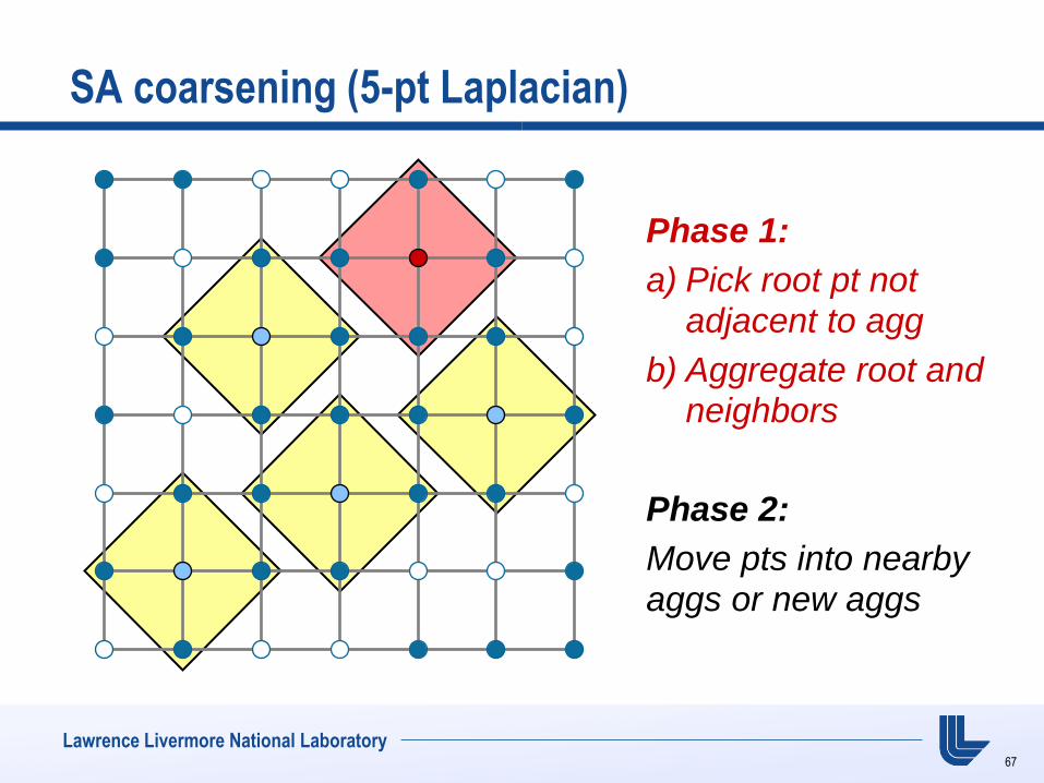
SA coarsening (5-pt Laplacian)
Phase 1:
a) Pick root pt not adjacent to agg
b) Aggregate root and neighbors
Phase 2:
Move pts into nearby
aggs or new aggs
62
Lawrence Livermore National Laboratory
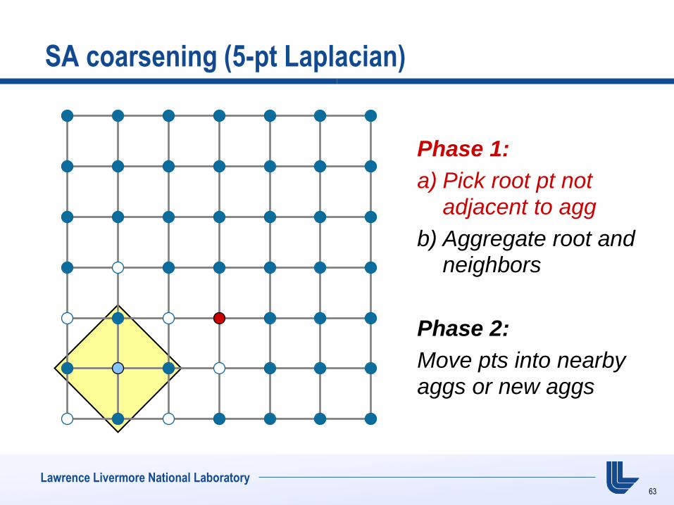
SA coarsening (5-pt Laplacian)
Phase 1:
a) Pick root pt not adjacent to agg
b) Aggregate root and neighbors
Phase 2:
Move pts into nearby
aggs or new aggs
63
Lawrence Livermore National Laboratory
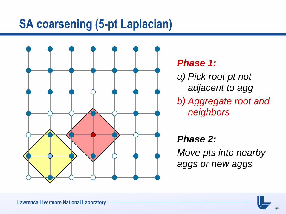
SA coarsening (5-pt Laplacian)
Phase 1:
a) Pick root pt not adjacent to agg
b) Aggregate root and neighbors
Phase 2:
Move pts into nearby
aggs or new aggs
64
Lawrence Livermore National Laboratory
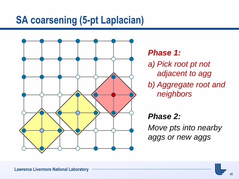
SA coarsening (5-pt Laplacian)
Phase 1:
a) Pick root pt not adjacent to agg
b) Aggregate root and neighbors
Phase 2:
Move pts into nearby
aggs or new aggs
65
Lawrence Livermore National Laboratory
SA coarsening (5-pt Laplacian)
Phase 1:
a) Pick root pt not adjacent to agg
b) Aggregate root and neighbors
Phase 2:
Move pts into nearby
aggs or new aggs
66
Lawrence Livermore National Laboratory
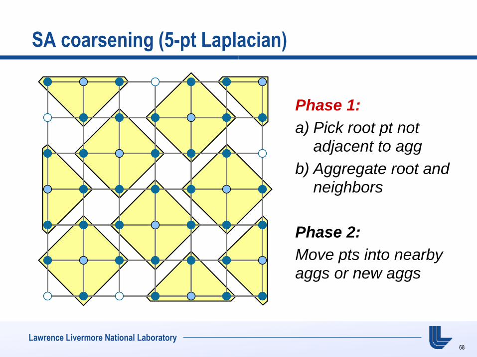
SA coarsening (5-pt Laplacian)
Phase 1:
a) Pick root pt not adjacent to agg
b) Aggregate root and neighbors
Phase 2:
Move pts into nearby
aggs or new aggs
67
Lawrence Livermore National Laboratory
SA coarsening (5-pt Laplacian)
Phase 1:
a) Pick root pt not adjacent to agg
b) Aggregate root and neighbors
Phase 2:
Move pts into nearby
aggs or new aggs
68
Lawrence Livermore National Laboratory
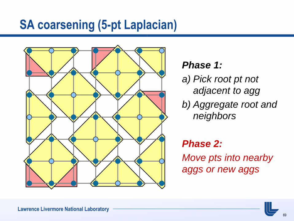
SA coarsening (5-pt Laplacian)
Phase 1:
a) Pick root pt not adjacent to agg
b) Aggregate root and neighbors
Phase 2:
Move pts into nearby
aggs or new aggs
69
Lawrence Livermore National Laboratory
SA coarsening (5-pt Laplacian)
Phase 1:
a) Pick root pt not adjacent to agg
b) Aggregate root and neighbors
Phase 2:
Move pts into nearby
aggs or new aggs
70
Lawrence Livermore National Laboratory
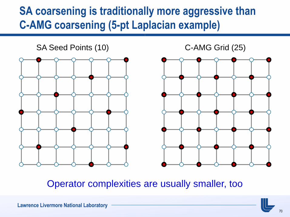
SA coarsening is traditionally more aggressive than
C-AMG coarsening (5-pt Laplacian example)
SA Seed Points (10) C-AMG Grid (25)
Operator complexities are usually smaller, too
71
Lawrence Livermore National Laboratory
Additional comments on SA…
Usual prolongator smoother is damped Jacobi
Strength of connection is usually defined differently
Special care must be taken for anisotropic problems to
keep complexity low
• Thresholded prolongator smoothing
• Basis shifting approach
Parallel SA coarsening has issues similar to C-AMG
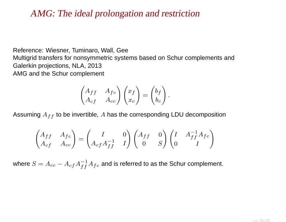
AMG: The ideal prolongation and restriction
Reference: Wiesner, Tuminaro, Wall, GeeMultigrid transfers for nonsymmetric systems based on Schur complements andGalerkin projections, NLA, 2013AMG and the Schur complement
(Aff Afc
Acf Acc
)(xf
xc
)=
(bf
bc
).
Assuming Aff to be invertible, A has the corresponding LDU decomposition
(Aff Afc
Acf Acc
)=
(I 0
AcfA−1ff
I
)(Aff 0
0 S
)(I A−1
ffAfc
0 I
)
where S = Acc −AcfA−1ff
Afc and is referred to as the Schur complement.
– p. 15/25
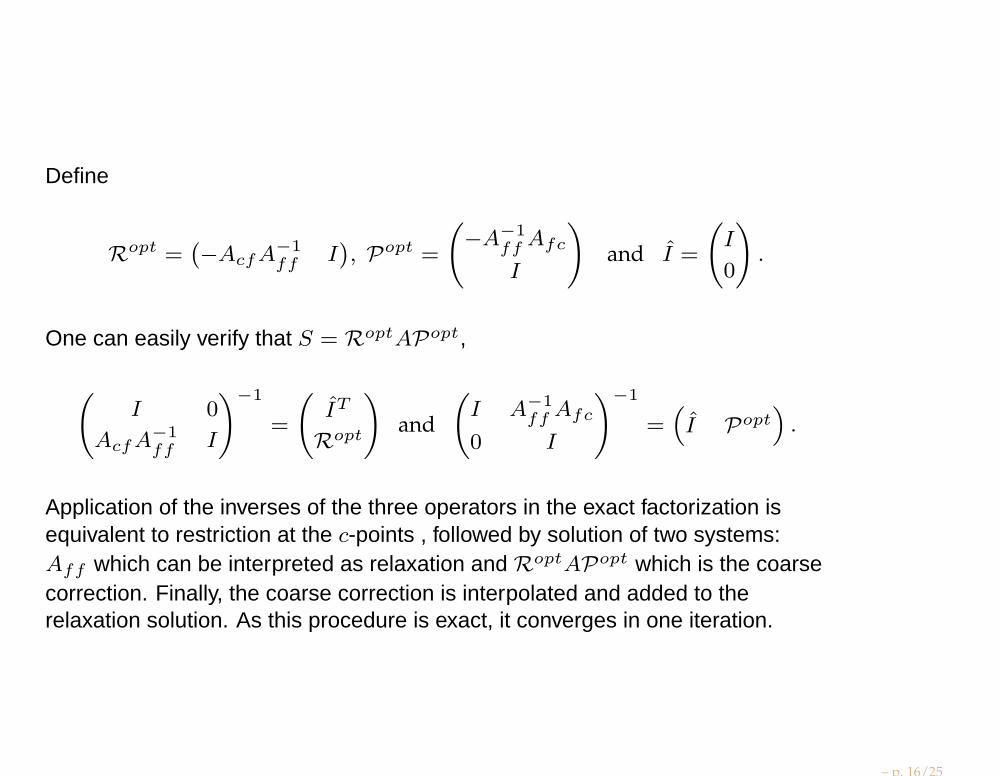
Define
Ropt =(−AcfA
−1ff
I), Popt =
(−A−1
ffAfc
I
)and I =
(I
0
).
One can easily verify that S = RoptAPopt,
(I 0
AcfA−1ff
I
)−1
=
(IT
Ropt
)and
(I A−1
ffAfc
0 I
)−1
=(I Popt
).
Application of the inverses of the three operators in the exact factorization isequivalent to restriction at the c-points , followed by solution of two systems:Aff which can be interpreted as relaxation and RoptAPopt which is the coarsecorrection. Finally, the coarse correction is interpolated and added to therelaxation solution. As this procedure is exact, it converges in one iteration.
– p. 16/25
Further work:how to approximate Ropt, Popt and S, or rather the coarse correction
RoptAPopt, which is nothing but AcfA−1ff
Afc.
We enter the full block factorized preconditioning framework, that can be seen aspurely algebraic and not related to MG.
– p. 17/25
TDB − NLA Algebraic Multilevel Iteration Methods (AMLI)
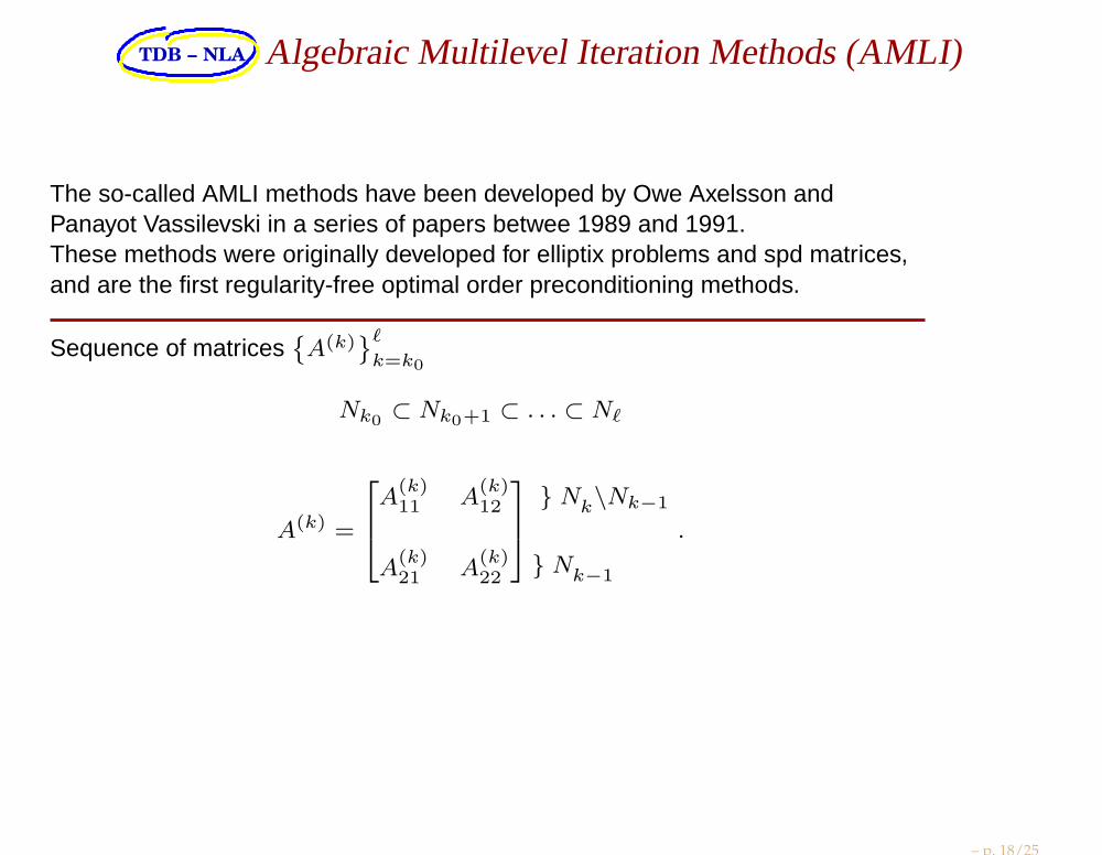
The so-called AMLI methods have been developed by Owe Axelsson andPanayot Vassilevski in a series of papers betwee 1989 and 1991.These methods were originally developed for elliptix problems and spd matrices,and are the first regularity-free optimal order preconditioning methods.
Sequence of matricesA(k)
ℓk=k0
Nk0⊂ Nk0+1 ⊂ . . . ⊂ Nℓ
A(k) =
A
(k)11 A
(k)12
A(k)21 A
(k)22
Nk\Nk−1
Nk−1
.
– p. 18/25
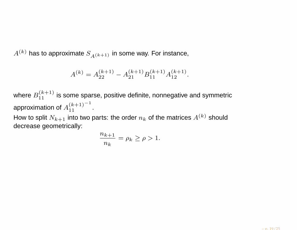
A(k) has to approximate SA(k+1) in some way. For instance,
A(k) = A(k+1)22 −A
(k+1)21 B
(k+1)11 A
(k+1)12 .
where B(k+1)11 is some sparse, positive definite, nonnegative and symmetric
approximation of A(k+1)−1
11 .
How to split Nk+1 into two parts: the order nk of the matrices A(k) shoulddecrease geometrically:
nk+1
nk
= ρk ≥ ρ > 1.
– p. 19/25
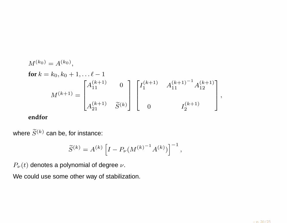
M(k0) = A(k0),
for k = k0, k0 + 1, . . . ℓ− 1
M(k+1) =
A(k+1)11 0
A(k+1)21 S(k)
I(k+1)1 A
(k+1)−1
11 A(k+1)12
0 I(k+1)2
,
endfor
where S(k) can be, for instance:
S(k) = A(k)[I − Pν(M
(k)−1A(k))
]−1
,
Pν(t) denotes a polynomial of degree ν.
We could use some other way of stabilization.
– p. 20/25
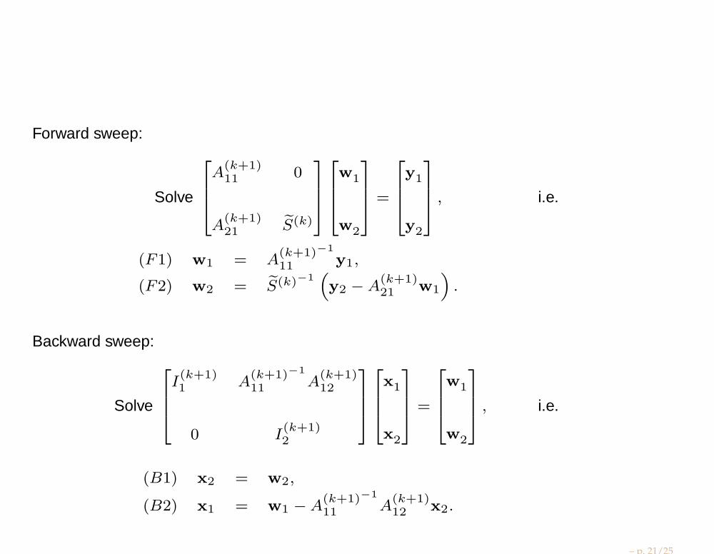
Forward sweep:
Solve
A(k+1)11 0
A(k+1)21 S(k)
w1
w2
=
y1
y2
, i.e.
(F1) w1 = A(k+1)−1
11 y1,
(F2) w2 = S(k)−1(y2 −A
(k+1)21 w1
).
Backward sweep:
Solve
I(k+1)1 A
(k+1)−1
11 A(k+1)12
0 I(k+1)2
x1
x2
=
w1
w2
, i.e.
(B1) x2 = w2,
(B2) x1 = w1 −A(k+1)−1
11 A(k+1)12 x2.
– p. 21/25
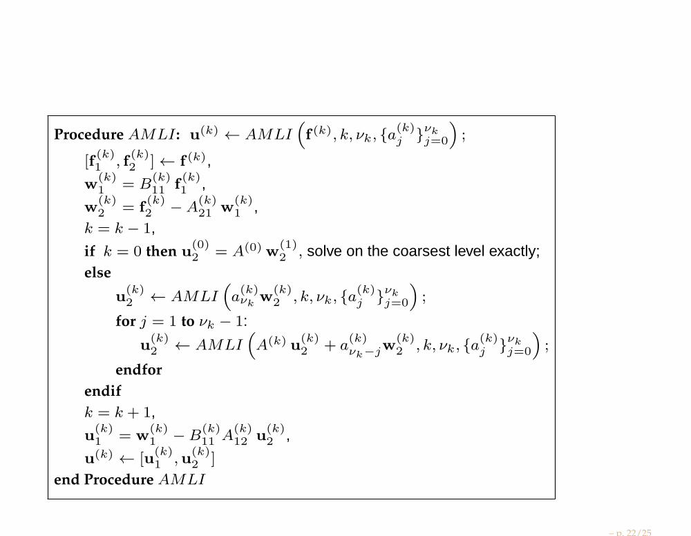
Procedure AMLI : u(k) ← AMLI(f (k), k, νk, a
(k)j
νkj=0
);
[f(k)1 , f
(k)2 ]← f (k),
w(k)1 = B
(k)11 f
(k)1 ,
w(k)2 = f
(k)2 −A
(k)21 w
(k)1 ,
k = k − 1,
if k = 0 then u(0)2 = A(0) w
(1)2 , solve on the coarsest level exactly;
else
u(k)2 ← AMLI
(a(k)νk w
(k)2 , k, νk, a
(k)j
νkj=0
);
for j = 1 to νk − 1:
u(k)2 ← AMLI
(A(k) u
(k)2 + a
(k)νk−jw
(k)2 , k, νk, a
(k)j
νkj=0
);
endfor
endif
k = k + 1,
u(k)1 = w
(k)1 −B
(k)11 A
(k)12 u
(k)2 ,
u(k) ← [u(k)1 ,u
(k)2 ]
end Procedure AMLI
– p. 22/25
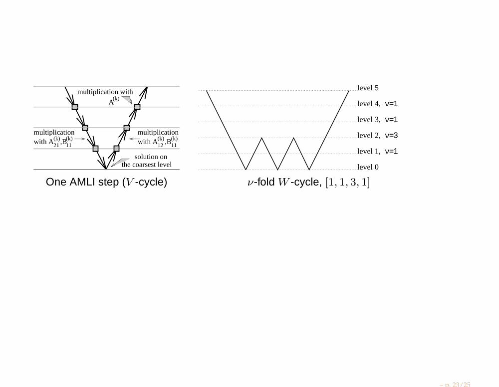
solution onthe coarsest level
multiplicationwith A(k)
12 ,B(k)11
multiplicationwith A(k)
21,B(k)11
multiplication with
A(k)
level 0
level 1,
level 2,
level 3,
level 4,
level 5
ν=1
ν=3
ν=1
ν=1
One AMLI step (V -cycle) ν-fold W -cycle, [1, 1, 3, 1]
– p. 23/25
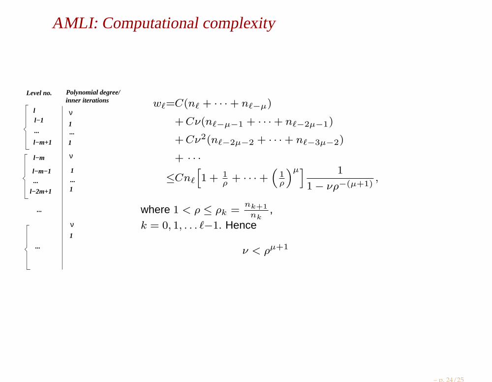
AMLI: Computational complexity
ll−1
...
l−m+1
l−m
...l−m−1
l−2m+1
...
...
ν
ν
ν
1
1
1
1...
...
1
Polynomial degree/inner iterations
Level no.
wℓ=C(nℓ + · · ·+ nℓ−µ)
+Cν(nℓ−µ−1 + · · ·+ nℓ−2µ−1)
+Cν2(nℓ−2µ−2 + · · ·+ nℓ−3µ−2)
+ · · ·
≤Cnℓ
[1 + 1
ρ+ · · ·+
(1ρ
)µ] 1
1− νρ−(µ+1),
where 1 < ρ ≤ ρk =nk+1
nk
,k = 0, 1, . . . ℓ−1. Hence
ν < ρµ+1
– p. 24/25

TDB − NLA Parallel Algorithms for Scientific Computing
Time to try ready packages!
– p. 25/25