Multilevel Agglomerative Edge Bundling for Visualizing Large Graphs

Emden R. Gansner∗ Yifan Hu∗ Stephen North∗ Carlos Scheidegger∗

AT&T Labs - Research, 180 Park Ave, Florham Park, NJ 07932.

ABSTRACT

Graphs are often used to encapsulate relationships between objects.Node-link diagrams, commonly used to visualize graphs, sufferfrom visual clutter on large graphs. Edge bundling is an effectivetechnique for alleviating clutter and revealing high-level edge pat-terns. Previous methods for general graph layouts either require acontrol mesh to guide the bundling process, which can introducehigh variation in curvature along the bundles, or all-to-all force andcompatibility calculations, which is not scalable. We propose amultilevel agglomerative edge bundling method based on a prin-cipled approach of minimizing ink needed to represent edges, withadditional constraints on the curvature of the resulting splines. Theproposed method is much faster than previous ones, able to bundlehundreds of thousands of edges in seconds, and one million edgesin a few minutes.1

Keywords: Edge bundling, multilevel, clustering, graph drawing.

Index Terms: I.3.3 [Computer Graphics]: Picture/ImageGeneration—Line and Curve Generation; I.3.5 [Computer Graph-ics]: Computational Geometry and Object Modeling—Hierarchyand Geometric Transformations

1 INTRODUCTION

Graphs are often used to model relationships between objects aris-ing in many application areas, such as social networks, biology,computer science and transportation. Node-link diagrams, in whichnodes are drawn as points and edges as straight lines, are commonlyemployed to visualize graphs. These visualizations are mostly de-termined by the position we choose to associate with each vertexof the graph. This mapping of vertices to position is the layout ofa graph. It is a truism that our ability to generate large data ex-ceeds our ability to visualize it, and this gap motivates the workwe present here. We are driven in part by the popularity of onlinesocial networks, as well as automated data acquisition techniquesin the sciences and social sciences. Scalable and high-quality algo-rithms exist to lay out very large graphs; these include multilevelforce-directed algorithms [6, 11, 15] and scalable multidimensionalscaling algorithms [3]. On many graphs, the node-link diagramsproduced by these algorithms are often aesthetically pleasing andreveal intrinsic structure of the graphs. However, on certain classesof graphs, a node-link diagram using straight edges is almost al-ways difficult to comprehend, with edges obstructing nodes andeach other. Often, the layout algorithms themselves are workingcorrectly, in the sense that removing edges from the visualizationcan reveal meaningful node clusters. It is the sheer number of edgesand their heterogeneous arrangement that clutter the visualization,hiding potential high-level patterns.

A number of approaches help reduce visual clutter. First, graphscan be simplified by coalescing clusters of nodes in a hierarchical

∗e-mail: {erg,yifanhu,north,cscheid}@research.att.com

1Additional images can be found at http://www2.research.

att.com/˜yifanhu/edge_bundling/.

fashion [25]. This can be combined with fisheye-style distortion tobalance high-level structures and local details [8]. Second, inter-active visualization systems [19] can be used to explore the graph,filtering out unnecessary visual artifacts.

A third useful tool is edge bundling. In this approach, edges arerepresented by deformable curves, typically cubic splines. Edgeswhich are in some sense close to each other are referred to as com-patible, and these compatible edges are then combined in a singlebundle, sharing part of their routes. This is analogous to electri-cal wires fanning into a bundle, and fanning out at the other end.Bundling reduces visual clutter, and helps reveal high-level nodeand edge patterns. Initially, edge bundling was proposed for circu-lar and hierarchical layout [7, 12, 21, 22], and was later extended togeneral graph layouts [5, 13, 18].

In this paper, we consider edge bundling for general undirectedlayouts. We propose a principled, efficient, and conceptually sim-ple edge bundling algorithm. The algorithm is similar to recent fastagglomerative clustering techniques [1, 23], except here we clustercompatible edges to save ink, as we will shortly explain. We werealso inspired by agglomerative bundling algorithms for circular lay-outs [7]. The major advance is that our algorithm works for generallayouts.

The guiding principle of our algorithm is saving ink [7]. Draw-ing a bundled group of edges should take less ink than drawingeach edge separately. Conceptually, the algorithm mimics the be-havior of a human faced with the task of bundling a mass of electri-cal wires: identifying wires that have similar start and end points;merging them; checking whether additional wires can join existingbundles or need to start new bundles; and repeating this process.

To avoid the cost of computing all-to-all edge interactions, asin the force-directed edge bundling algorithm FDEB [13], we firstconstruct a proximity graph of edges. Guided by this graph, wethen check whether bundling each edge with its neighbors savesink. When all possible bundlings are identified, we form a coarseedge proximity graph based on the edge grouping, and repeat thebundling process on this graph. After no more ink saving is pos-sible, we fix the fan-in and fan-out parts of the edges (as shownin Figure 1), and consider the bundled parts of the edges to see ifthe aforementioned edge bundling procedure can be applied to thebundled parts recursively. Curvature is controlled by restricting theturning angles when an edge joins a bundle. Applying this algo-rithm to many real-world graphs results in fast edge bundling thatreveals high-level edge patterns.

The remainder of this paper is organized as follows. In Section 2,we review related work. Section 3 introduces the multilevel ag-glomerative edge bundling algorithm, followed by Section 4, wherewe introduce GPU-based rendering methods for faster interactivemanipulation. The section provides example visualizations, includ-ing some for very large graphs. We conclude the paper in Section 5with topics for further research.

2 RELATED WORK

Early work on edge bundling focused on special classes of graphlayouts. Newbery [22] proposed a method for handling layeredlayouts of directed graphs. The method identifies edges that forma complete bipartite graph, and makes these edges pass through acommon dummy node, thus eliminating many crossings. A modi-

fication of this was implemented in Graphviz [9]. Holten’s Hier-archical Edge Bundling (HEB) [12] works with graphs that have adefined hierarchy. It bundles edges using B-splines, following thecontrol points defined by the hierarchy. Gansner et al. [7] presentedan algorithm that reduces clutter in circular layouts by mergingedges so that the resulting splines share some control points. In ourwork, we adopt their model of minimizing the total amount of inkneeded to draw the edges. This objective is incorporated in our al-gorithm. Finally, Nachmanson et al. [21] consider edge bundling inlayered drawings with edges already routed as polylines or splines.The goal of uncluttering the drawing is balanced with preservingthe topology of the original drawing and disambiguating edges.

Cui et al. [5] proposed one of the first methods suitable for gen-eral undirected layouts. In the Geometry Based Edge Bundling(GBEB) method, a control mesh guides the edge-clustering pro-cess; edge bundles are formed by forcing all edges to pass throughthe same control points on the mesh. The algorithm was reported tobe fast, although the resulting visualization was observed to exhibita “webbing” effect [13], with edges having high curvature varia-tions.

Holten and van Wijk proposed a Force-Directed Edge Bundling(FDEB) algorithm [13]. The algorithm is conceptually simple, uti-lizing edges modeled as flexible springs that can attract each other.The attractive force is proportional to the inverse (or inverse square)distance of the springs, as well as to the compatibility of the edges.It was found to result in smoother bundles that are easy to read.A weakness of this algorithm is its high computational complexity.The authors suggested that a Barnes-Hut like subdivision-based ap-proach may be used to speed up the algorithm, though no details onhow this can be done were given.

Lambert et al. [18] proposed an edge bundling algorithm that isalso based on the use of a mesh. Graph edges are routed alongmesh edges using a shortest path algorithm. Mesh edge weightsare updated to encourage more graph edges to share common meshedges. The algorithm was found to be faster than force-directededge bundling [13]. Further optimization in the use of shortest pathalgorithm and in parallelization made its speed close to that of thegeometry-based bundling algorithm [5]. The method was subse-quently extended to 3D [17].

3 MULTILEVEL AGGLOMERATIVE EDGE BUNDLING

Throughout this paper we assume that we are working with a graphG= {V, E}, with |V | vertices and |E| edges. We assume that we aremaking 2D drawings, and that the positions of vertices are given.The proposed algorithm is readily extended to 3D.

As discussed in Section 1, our intuition is to mimic what a hu-man operator would do when faced with the task of bundling a massof electrical wires: identify wires that have similar start and endpoints; merge them; check if additional wires can join existing bun-dles, or need to start their own; and repeat this process. To achievethis, we must first identify edges that are “similar.” Holten and vanWijk [13] introduced four edge compatibility measures. For eachedge, a naive way to find similar edges is to check every other edgefor compatibility, an |E|2 operation.

However, we are interested in an edge bundling algorithm thatcan scale to very large graphs, so we must avoid the quadratic com-plexity involved in making such an all-to-all similarity computa-tion. Our solution is to use a simple compatibility measure whereeach edge is treated as a point in 4-dimensional space, and edge-edge similarity is given by a metric in that space. Within this set-ting, we can form an edge proximity graph efficiently. Edges thatare neighbors in the proximity graph can then be checked for pos-sible bundling. Edges that are not immediate neighbors can still bebundling in the multilevel process described in Section 3.3. Theoverall algorithm is illustrated in Figure 1, and described in detailin the following.

3.1 Edge proximity graph

Each vertex u has a position in 2D denoted as xu. We representeach edge (u,v) as a 4-dimensional vector (xu,xv). Two edges are“close” if their Euclidean distance in the 4-dimensional space issmall. A space decomposition, e.g., a kd-tree, can be constructedusing all |E| 4-dimensional vectors in time |E|log(|E|). This datastructure then allows us to find the k-nearest (k << |E|) neighborsin time k log(|E|) per edge. Thus we construct an edge proximitygraph Γ in time k|E|log(|E|). We note that ordering of the pointsin the 4-dimensional vector (xu,xv) affects the distance in the em-bedding. This effect can be avoided by ordering the 4-dimensionalvector based on the x− or y− coordinates, or simply by insertingboth (xu,xv) and (xv,xu) in the data structure, without affecting thek|E|log(|E|) complexity. We stress here that vertices in Γ and G arenot the same: vertices of Γ are edges of G.

An edge proximity graph Γ so constructed may not treat all com-patible edges as neighbors, both because of the limited number k ofneighbors considered, and because we measure proximity using theEuclidean norm in 4D, instead of using more detailed compatibil-ity measures [13] that take into account length, angle, position, andvisibility. This, however, does not cause significant problems, be-cause we ultimately measure the compatibility of edges by whetherbundling results in saving ink. In addition, our multilevel bundlingprocess can bundle not only neighbors, but a neighbor’s neighbors,etc. Finally, a recursive process further increases the opportunityto bundle edges that were not initially considered as being close.Figure 1 (b) shows the edge proximity graph corresponding to theedges in Figure 1 (a).

3.2 Agglomerative bundling

Once Γ is constructed, it guides the bundling decisions. For eachneighbor v of a vertex u in Γ, we calculate the ink saving that mayresult if the edge represented by v is bundled with the edge rep-resented by u. We then choose among all u’s neighbors one thatgives the maximal ink saving. Note that a neighbor v may alreadybe bundled with other edges, in which case v represents a bundle.Let e(u) denote the edge or edges represented by a node u in Γ.Let ink(e(u)) denote the ink needed to draw the edge (or bundle ofedges) represented by u, and e(u)∪ e(v) an edge bundle formed bymerging the edges represented by u and v. Then the amount of inksaved by bundling the edges is defined as

ink(e(u))+ ink(e(v))− ink(e(u)∪ e(v))

We calculate the (approximate) minimal amount of ink neededto draw a set of edges using the one dimensional optimizationprocedure of Gansner and Koren [7]. Given the set of edgese(u)∪ e(v) = {e1 = (xS

1,xT1 ),e2 = (xS

2,xT2 ), . . . ,ek = (xS

k ,xTk )}. As-

sume that the ends of the edges are properly ordered so that theyform two equal sized sets, the source set S = {xS

1,xS2, . . . ,x

Sk} and

the target set T = {xT1 ,x

T2 , . . . ,x

Tk }. The aim of the ink optimization

procedure is to find two meeting points M1 and M2, such that edgesleaving nodes in the source set S fan-in to M1, travel along a straightline to M2, then fan-out to nodes in the target set T (Figure 2). Thetotal ink used to draw these edges is

f (S,T,M1,M2) = ∑x∈S

||x−M1||+ ||M1−M2||+ ∑x∈T

||M2−x||. (1)

The meeting points M1 and M2 are chosen to minimize the total ink,

ink(e(u)∪ e(v)) = minM1,M2

f (S,T,M1,M2).

The following heuristic is used to find the approximate optimalmeeting points. First, the centroids of the sets S and T are com-puted. Then, we minimize (1) by the procedure known as golden

1234

5 67 8 9 10

→

1

2

3

4

5

67

89

10

→ →

81, 2< 83, 4<

85, 6< 87, 8< 89, 10<

(a) (b) (c) (d)

→ → →

(e) (f) (g) (h)

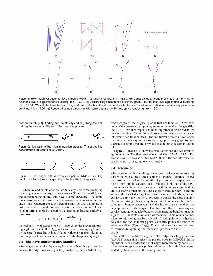
Figure 1: How multilevel agglomerative bundling works: (a) Original edges. Ink = 35.82. (b) Constructing an edge proximity graph (k = 3). (c)After one level of agglomerative bundling. Ink = 19.31. (d) Constructing a coarsened proximity graph. (e) After multilevel agglomerative bundling.Ink = 12.00. We call the tree-like branching portions of the bundles at their endpoints the fan-in and fan-out. (f) After recursive application ofbundling. Ink = 10.94. (g) Rendered using splines. (h) With turning angle <= 40o and spline rendering. Ink = 15.24.

section search [24], finding two points M1 and M2 along the linelinking the centroids. Figure 2 illustrates the process.

Figure 2: Illustration of the ink minimization process. The dotted linepass through the centroids of S and T .

Figure 3: Left: edges with far away end points. Middle: bundlingresults in a large turning angle. Right: limiting the turning angle.

When the end points of edges are far away, sometimes bundlingthese edges results in large turning angles (Figure 3, middle), andthe corresponding splines will have a large curvature. We avoidthis in two ways. First, we allow a user-specified maximum turningangle, and constrain the two meeting points so that this angle isnot exceeded. Second, we compromise between saving ink andsmaller turning angle by selecting the meeting points M1 and M2 tominimize

f (S,T,M1,M2)

(

1+cos(Amax)

p

)

,

instead of (1), with parameter p > 1, subject to the maximum turn-ing angle constraint. Here Amax is the maximum turning angle givenby the specific meeting points. A larger value of p makes ink savingmore important, while a smaller value avoids sharp turning angles.

3.3 Multilevel agglomerative bundling

After edges are bundled by the agglomerative bundling process, wecoarsen the edge proximity graph by coalescing nodes (which rep-

resent edges of the original graph) that are bundled. Now eachnode of the coarsened graph may represent a bundle of edges (Fig-ure 1 (d)). We then repeat the bundling process described in theprevious section. This multilevel process terminates when no moreink saving can be identified. The multilevel process allows edgesthat may be far away in the original edge proximity graph to havea chance to form a bundle, provided that doing so results in savingink.

Figures 1 (c) and 1 (e) show the results after one and two levels ofagglomeration. The first level reduces ink from 35.82 to 19.31. Thesecond level reduces it further to 12.00. No further ink reductioncan be achieved by going one level further.

3.4 Recursion

After one step of this bundling process, each edge is represented bya polyline with at most three segments. Figure 4 (middle) showsthe result at the end of the multilevel process when applied to theairlines graph (see Section 4). While a single step of the algo-rithm reduces clutter when compared with the original graph, thereare still many similar splines that can be merged further. Thereforewe take the bundled straight sections as a new set of edges, and re-cursively apply the multilevel process to bundle the edge bundles.To promote straight lines, weights are used to represent the numberof edges a bundle represents, and the ink to draw a bundled lineis proportional to its weight. This has the effect of avoiding ex-cessive bending of heavier bundles when merging bundles together.Figure 1 (f) illustrates the result of recursion. This recursion endswhen no ink saving can be achieved. At this point each edge is apolyline. We use the turning points as control points and render theedges as splines (Figure 1 (g)). Figure 4 (bottom) shows the resultof recursively applying the multilevel process to the airlines

graph.

We call this multilevel agglomerative edge bundling procedureMINGLE. Algorithm 1 gives the pseudo-code for MINGLE. In thealgorithm, e(v) denotes the set of edges represented by node v. Ifv has been assigned a group, then this set also include edges repre-sented by those nodes in the same group as v.

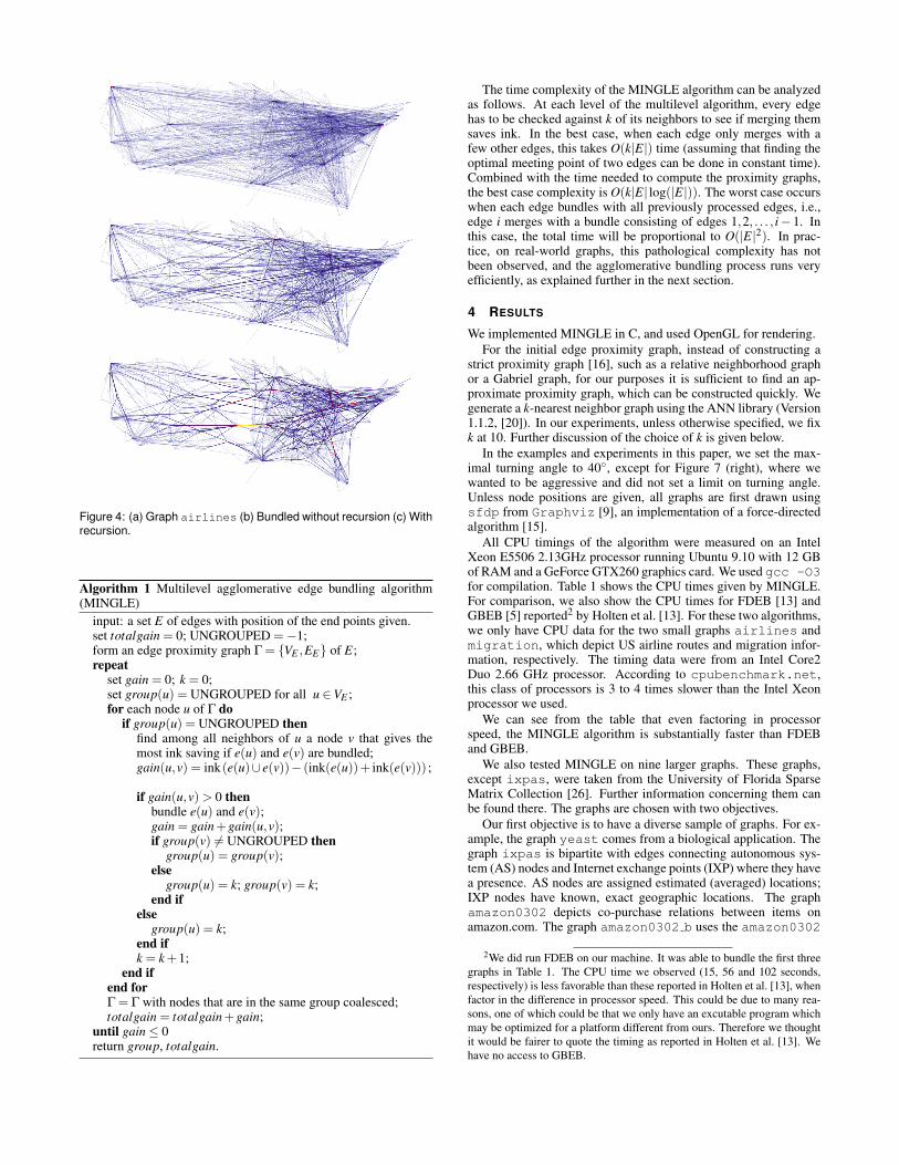
Figure 4: (a) Graph airlines (b) Bundled without recursion (c) Withrecursion.

Algorithm 1 Multilevel agglomerative edge bundling algorithm(MINGLE)

input: a set E of edges with position of the end points given.set totalgain = 0; UNGROUPED =−1;form an edge proximity graph Γ = {VE ,EE} of E;repeat

set gain = 0; k = 0;set group(u) = UNGROUPED for all u ∈VE ;for each node u of Γ do

if group(u) = UNGROUPED thenfind among all neighbors of u a node v that gives themost ink saving if e(u) and e(v) are bundled;gain(u,v) = ink(e(u)∪ e(v))− (ink(e(u))+ ink(e(v))) ;

if gain(u,v)> 0 thenbundle e(u) and e(v);gain = gain+gain(u,v);if group(v) 6= UNGROUPED then

group(u) = group(v);else

group(u) = k; group(v) = k;end if

elsegroup(u) = k;

end ifk = k+1;

end ifend forΓ = Γ with nodes that are in the same group coalesced;totalgain = totalgain+gain;

until gain ≤ 0return group, totalgain.

The time complexity of the MINGLE algorithm can be analyzedas follows. At each level of the multilevel algorithm, every edgehas to be checked against k of its neighbors to see if merging themsaves ink. In the best case, when each edge only merges with afew other edges, this takes O(k|E|) time (assuming that finding theoptimal meeting point of two edges can be done in constant time).Combined with the time needed to compute the proximity graphs,the best case complexity is O(k|E| log(|E|)). The worst case occurswhen each edge bundles with all previously processed edges, i.e.,edge i merges with a bundle consisting of edges 1,2, . . . , i− 1. Inthis case, the total time will be proportional to O(|E|2). In prac-tice, on real-world graphs, this pathological complexity has notbeen observed, and the agglomerative bundling process runs veryefficiently, as explained further in the next section.

4 RESULTS

We implemented MINGLE in C, and used OpenGL for rendering.

For the initial edge proximity graph, instead of constructing astrict proximity graph [16], such as a relative neighborhood graphor a Gabriel graph, for our purposes it is sufficient to find an ap-proximate proximity graph, which can be constructed quickly. Wegenerate a k-nearest neighbor graph using the ANN library (Version1.1.2, [20]). In our experiments, unless otherwise specified, we fixk at 10. Further discussion of the choice of k is given below.

In the examples and experiments in this paper, we set the max-imal turning angle to 40◦, except for Figure 7 (right), where wewanted to be aggressive and did not set a limit on turning angle.Unless node positions are given, all graphs are first drawn usingsfdp from Graphviz [9], an implementation of a force-directedalgorithm [15].

All CPU timings of the algorithm were measured on an IntelXeon E5506 2.13GHz processor running Ubuntu 9.10 with 12 GBof RAM and a GeForce GTX260 graphics card. We used gcc -O3

for compilation. Table 1 shows the CPU times given by MINGLE.For comparison, we also show the CPU times for FDEB [13] andGBEB [5] reported2 by Holten et al. [13]. For these two algorithms,we only have CPU data for the two small graphs airlines andmigration, which depict US airline routes and migration infor-mation, respectively. The timing data were from an Intel Core2Duo 2.66 GHz processor. According to cpubenchmark.net,this class of processors is 3 to 4 times slower than the Intel Xeonprocessor we used.

We can see from the table that even factoring in processorspeed, the MINGLE algorithm is substantially faster than FDEBand GBEB.

We also tested MINGLE on nine larger graphs. These graphs,except ixpas, were taken from the University of Florida SparseMatrix Collection [26]. Further information concerning them canbe found there. The graphs are chosen with two objectives.

Our first objective is to have a diverse sample of graphs. For ex-ample, the graph yeast comes from a biological application. Thegraph ixpas is bipartite with edges connecting autonomous sys-tem (AS) nodes and Internet exchange points (IXP) where they havea presence. AS nodes are assigned estimated (averaged) locations;IXP nodes have known, exact geographic locations. The graphamazon0302 depicts co-purchase relations between items onamazon.com. The graph amazon0302 b uses the amazon0302

2We did run FDEB on our machine. It was able to bundle the first three

graphs in Table 1. The CPU time we observed (15, 56 and 102 seconds,

respectively) is less favorable than these reported in Holten et al. [13], when

factor in the difference in processor speed. This could be due to many rea-

sons, one of which could be that we only have an excutable program which

may be optimized for a platform different from ours. Therefore we thought

it would be fairer to quote the timing as reported in Holten et al. [13]. We

have no access to GBEB.

name |E| MINGLE FDEB* GBEB*

airlines 1297 0.1 19 2.5yeast 6646 0.9 - -migration 9660 1.0 80 18.8wiki-Vote 100762 18.4 - -ixpas 149661 32.3 - -net50 464440 87.1 - -amazon0302 899792 277. - -net100 1001640 204. - -amazon0302 b 1233364 267. - -net150 1538840 355. - -Stanford 1992636 404. - -pattern1 4652095 1049. - -

Table 1: CPU time (in seconds) taken by different edge bundling al-gorithms. Columns marked with an asterisk (*) show CPU times froma processor that is 3-4 times slower than the one used for MINGLE.

name source |V | % inksaving

avg.work

airlines [5, 13] 235 59.2 126.4yeast [26] 2361 45.1 206.6migration* [5, 13] 6517 74.5 137.8wiki-Vote [26] 8297 66.8 173.5ixpas AT&T 28546 90.5 230.4net50 [26] 16320 81.5 164.3amazon0302 [26] 262111 54.8 240.7net100 [26] 29920 85.3 164.0amazon0302 b [26] 519010 55.8 207.9net150 [26] 43520 83.9 192.5Stanford [26] 281903 69.7 196.1pattern1 [26] 19242 84.5 176.2

Table 2: Additional measurements of MINGLE on test cases. “Inksaving” is percentage of ink saved when edges are bundled, insteadof drawn as straight edges. “Work” is average number of ink optimiza-tions each edge, or bundle, is involved in. ∗The migration graphcontains two-way edges that represent two-way migrations, and theduplication amount to 21.9% of total ink. Subtracting this, the ink sav-ing for the migration graph is 52.6.

matrix, but treats the rows and columns as two separate sets of ver-tices, thus yielding a bipartite graph.

The second objective is to have a wide range of number of edgesso as to test the scalability of MINGLE. To that end we selectednet50, net100, net150, three graphs of the same kind butdifferent sizes.

As can be seen, MINGLE is able to bundle graphs with around100,000 edges in about 20 seconds, and graphs with around onemillion edges in around 4 minutes. The largest graph, pattern1,has 4.6 million edges, and MINGLE processes it in 14 minutes.Overall, the algorithm scales well.

Table 2 gives some additional details about the graphs, and aboutMINGLE. It shows the percentage of ink saved, defined as,

ink to draw straight edges− ink to draw bundled edges

ink to draw straight edges,

in percentage. It also shows “average work”, a measure of the av-erage number of times an edge, or a bundle, is involved in ink opti-mization. Every time the ink optimization routine is invoked to findoptimal bundle for m edges or bundles, we increment “work” by m.The total “work” is divided by the number of edges in the originalgraph to get the “average work”. We can see that this quantity re-mains relatively stable as number of edges increases (rows in both

tables 1-2 are ordered by increasing number of edges). Given thatthe majority of CPU time is spent in the ink optimization proce-dure, the relatively stable “average work” shows that algorithm isnot exhibiting the worst case quadratic time complexity.

While all above results are based on k = 10, we experimentedwith values of k between 2 to 1000. Table 3 shows the amount ofink saving and CPU time for six graphs of varying sizes. Clearly,a relatively small k is sufficient to achieve good ink saving. Sur-prisingly, increasing k beyond a small value actually reduces inksaving, and increases CPU time. We do not know the exact reasonwhy ink saving actually deteriorate as k increases beyond 3. But webelieve that a smaller k prevents bundling of multiple edges at anearly stage of the multilevel agglomerative bundling process. Thiscreate a more balanced tree and promotes consideration of mergingcandidates that are not consider very close in the 4D space.

We choose a conservative k = 10 for results in Table 1-2 as weare aware that for artificial data, e.g., two sets of m parallel lineseach, with a small separating distance between the sets, a smallerk < m will yield a disconnected proximity graph. Although MIN-GLE will run fine on this example, the disconnected proximitygraph does prevent edges between the two sets to have a chanceto merge. But in practice, for the graphs tested in Table 3, k = 3seems to be a good choice. Overall, this experiment confirms thata small k does not hurt performance because of the local nature ofk-nearest neighbor graph, rather, the multilevel agglomerative pro-cess is robust and does provide the global reach needed.

k 2 3 5 10 50 100 1000

airl. 57.1 62.3 61.4 59.2 55.6 53.5 48.750.1 0.05 0.08 0.14 0.5 0.86 3.9

migra. 72.3 77.1 75.7 74.5 72.5 71.6 68.10.7 0.5 0.64 1.0 3.9 6.4 51.5

wiki. 60.5 68.8 67.5 66.8 64.7 63.5 63.59.5 5.7 11.4 18.4 70.3 127 391

amaz. 48.5 57.4 56.0 54.8 - - -262 157 177 277 - - -

net15. 86.2 84.5 83.9 83.0 - - -85 112 355 1257 - - -

patt. 70.6 87.4 85.2 84.5 - - -516 407 520 1049 - - -

Table 3: Effect of k on the ink saving and CPU time. In each cell,the top number is the percentage of ink saving; the bottom numberis CPU time (seconds). Cells marked with “-” mean that CPU timeexceeds 1500 seconds. It is seen that a relatively small k (e.g., k = 3)is better than very large k, and gives a larger ink saving and smallerCPU time. (The names of graphs are abbreviated to save space.)

4.1 Rendering

Similar to Holten and van Wijk [13], we use a GPU-based, OpenGLrendering technique to highlight edge bundles. We use the standardtechnique of additive alpha blending with a floating-point frame-buffer object to accurately count the number of edges incident oneach pixel, typically called the overdraw, which we will model asa scalar field ω : D ⊂ R2 → R (D denotes the screen rectangle). Todetermine the color of each pixel, we first find the maximum over-draw M = maxx∈D ω(x) using the standard procedure of reductionon the GPU [4]. We then use a linear colormap that encodes theoverdraw as a function from [0,M] → RGB. We use a blue-red-yellow-white palette for light backgrounds and a light-cyan-red-yellow-white palette for dark backgrounds.

Holten and van Wijk [13] suggest a continuous interpolation be-tween straight edges and bundled edges as a way for user to under-stand the bundle structure. We adopt that approach. Specifically,

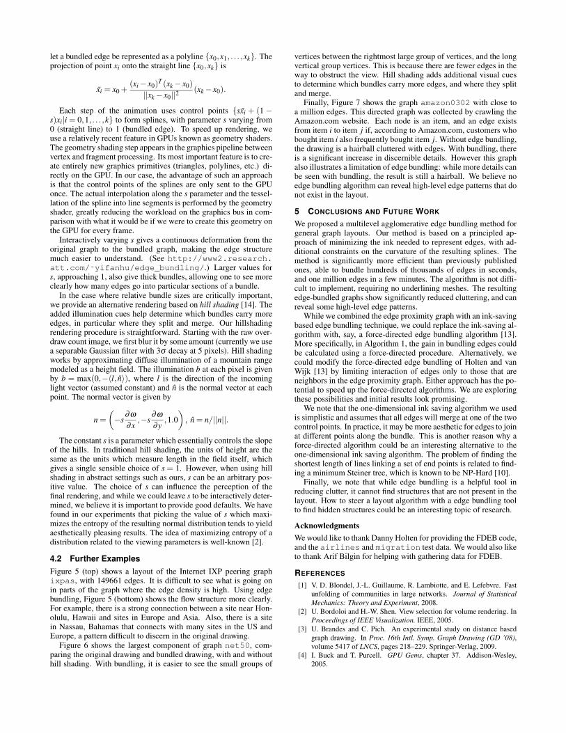
let a bundled edge be represented as a polyline {x0,x1, . . . ,xk}. Theprojection of point xi onto the straight line {x0,xk} is

xi = x0 +(xi − x0)

T (xk − x0)

||xk − x0||2(xk − x0).

Each step of the animation uses control points {sxi + (1 −s)xi|i = 0,1, . . . ,k} to form splines, with parameter s varying from0 (straight line) to 1 (bundled edge). To speed up rendering, weuse a relatively recent feature in GPUs known as geometry shaders.The geometry shading step appears in the graphics pipeline betweenvertex and fragment processing. Its most important feature is to cre-ate entirely new graphics primitives (triangles, polylines, etc.) di-rectly on the GPU. In our case, the advantage of such an approachis that the control points of the splines are only sent to the GPUonce. The actual interpolation along the s parameter and the tessel-lation of the spline into line segments is performed by the geometryshader, greatly reducing the workload on the graphics bus in com-parison with what it would be if we were to create this geometry onthe GPU for every frame.

Interactively varying s gives a continuous deformation from theoriginal graph to the bundled graph, making the edge structuremuch easier to understand. (See http://www2.research.

att.com/˜yifanhu/edge_bundling/.) Larger values fors, approaching 1, also give thick bundles, allowing one to see moreclearly how many edges go into particular sections of a bundle.

In the case where relative bundle sizes are critically important,we provide an alternative rendering based on hill shading [14]. Theadded illumination cues help determine which bundles carry moreedges, in particular where they split and merge. Our hillshadingrendering procedure is straightforward. Starting with the raw over-draw count image, we first blur it by some amount (currently we usea separable Gaussian filter with 3σ decay at 5 pixels). Hill shadingworks by approximating diffuse illumination of a mountain rangemodeled as a height field. The illumination b at each pixel is givenby b = max(0,−〈l, n〉), where l is the direction of the incominglight vector (assumed constant) and n is the normal vector at eachpoint. The normal vector is given by

n =

(

−s∂ω

∂x,−s

∂ω

∂y,1.0

)

, n = n/||n||.

The constant s is a parameter which essentially controls the slopeof the hills. In traditional hill shading, the units of height are thesame as the units which measure length in the field itself, whichgives a single sensible choice of s = 1. However, when using hillshading in abstract settings such as ours, s can be an arbitrary pos-itive value. The choice of s can influence the perception of thefinal rendering, and while we could leave s to be interactively deter-mined, we believe it is important to provide good defaults. We havefound in our experiments that picking the value of s which maxi-mizes the entropy of the resulting normal distribution tends to yieldaesthetically pleasing results. The idea of maximizing entropy of adistribution related to the viewing parameters is well-known [2].

4.2 Further Examples

Figure 5 (top) shows a layout of the Internet IXP peering graphixpas, with 149661 edges. It is difficult to see what is going onin parts of the graph where the edge density is high. Using edgebundling, Figure 5 (bottom) shows the flow structure more clearly.For example, there is a strong connection between a site near Hon-olulu, Hawaii and sites in Europe and Asia. Also, there is a sitein Nassau, Bahamas that connects with many sites in the US andEurope, a pattern difficult to discern in the original drawing.

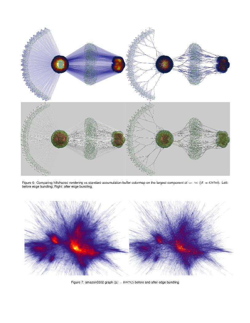
Figure 6 shows the largest component of graph net50, com-paring the original drawing and bundled drawing, with and withouthill shading. With bundling, it is easier to see the small groups of

vertices between the rightmost large group of vertices, and the longvertical group vertices. This is because there are fewer edges in theway to obstruct the view. Hill shading adds additional visual cuesto determine which bundles carry more edges, and where they splitand merge.

Finally, Figure 7 shows the graph amazon0302 with close toa million edges. This directed graph was collected by crawling theAmazon.com website. Each node is an item, and an edge existsfrom item i to item j if, according to Amazon.com, customers whobought item i also frequently bought item j. Without edge bundling,the drawing is a hairball cluttered with edges. With bundling, thereis a significant increase in discernible details. However this graphalso illustrates a limitation of edge bundling: while more details canbe seen with bundling, the result is still a hairball. We believe noedge bundling algorithm can reveal high-level edge patterns that donot exist in the layout.

5 CONCLUSIONS AND FUTURE WORK

We proposed a multilevel agglomerative edge bundling method forgeneral graph layouts. Our method is based on a principled ap-proach of minimizing the ink needed to represent edges, with ad-ditional constraints on the curvature of the resulting splines. Themethod is significantly more efficient than previously publishedones, able to bundle hundreds of thousands of edges in seconds,and one million edges in a few minutes. The algorithm is not diffi-cult to implement, requiring no underlining meshes. The resultingedge-bundled graphs show significantly reduced cluttering, and canreveal some high-level edge patterns.

While we combined the edge proximity graph with an ink-savingbased edge bundling technique, we could replace the ink-saving al-gorithm with, say, a force-directed edge bundling algorithm [13].More specifically, in Algorithm 1, the gain in bundling edges couldbe calculated using a force-directed procedure. Alternatively, wecould modify the force-directed edge bundling of Holten and vanWijk [13] by limiting interaction of edges only to those that areneighbors in the edge proximity graph. Either approach has the po-tential to speed up the force-directed algorithms. We are exploringthese possibilities and initial results look promising.

We note that the one-dimensional ink saving algorithm we usedis simplistic and assumes that all edges will merge at one of the twocontrol points. In practice, it may be more aesthetic for edges to joinat different points along the bundle. This is another reason why aforce-directed algorithm could be an interesting alternative to theone-dimensional ink saving algorithm. The problem of finding theshortest length of lines linking a set of end points is related to find-ing a minimum Steiner tree, which is known to be NP-Hard [10].

Finally, we note that while edge bundling is a helpful tool inreducing clutter, it cannot find structures that are not present in thelayout. How to steer a layout algorithm with a edge bundling toolto find hidden structures could be an interesting topic of research.

Acknowledgments

We would like to thank Danny Holten for providing the FDEB code,and the airlines and migration test data. We would also liketo thank Arif Bilgin for helping with gathering data for FDEB.

REFERENCES

[1] V. D. Blondel, J.-L. Guillaume, R. Lambiotte, and E. Lefebvre. Fast

unfolding of communities in large networks. Journal of Statistical

Mechanics: Theory and Experiment, 2008.

[2] U. Bordoloi and H.-W. Shen. View selection for volume rendering. In

Proceedings of IEEE Visualization. IEEE, 2005.

[3] U. Brandes and C. Pich. An experimental study on distance based

graph drawing. In Proc. 16th Intl. Symp. Graph Drawing (GD ’08),

volume 5417 of LNCS, pages 218–229. Springer-Verlag, 2009.

[4] I. Buck and T. Purcell. GPU Gems, chapter 37. Addison-Wesley,

2005.

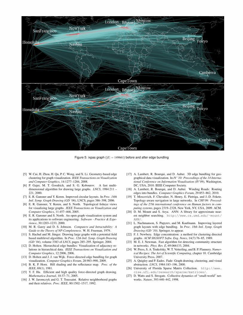
Figure 5: ixpas graph (|E|= 149661) before and after edge bundling

[5] W. Cui, H. Zhou, H. Qu, P. C. Wong, and X. Li. Geometry-based edge

clustering for graph visualization. IEEE Transactions on Visualization

and Computer Graphics, 14:1277–1284, 2008.

[6] P. Gajer, M. T. Goodrich, and S. G. Kobourov. A fast multi-

dimensional algorithm for drawing large graphs. LNCS, 1984:211 –

221, 2000.

[7] E. R. Gansner and Y. Koren. Improved circular layouts. In Proc. 14th

Intl. Symp. Graph Drawing (GD ’06), LNCS, pages 386–398, 2006.

[8] E. R. Gansner, Y. Koren, and S. North. Topological fisheye views

for visualizing large graphs. IEEE Transactions on Visualization and

Computer Graphics, 11:457–468, 2005.

[9] E. R. Gansner and S. North. An open graph visualization system and

its applications to software engineering. Software - Practice & Expe-

rience, 30:1203–1233, 2000.

[10] M. R. Garey and D. S. Johnson. Computers and Intractability: A

Guide to the Theory of NP-Completeness. W. H. Freeman, 1979.

[11] S. Hachul and M. Junger. Drawing large graphs with a potential field

based multilevel algorithm. In Proc. 12th Intl. Symp. Graph Drawing

(GD ’04), volume 3383 of LNCS, pages 285–295. Springer, 2004.

[12] D. Holten. Hierarchical edge bundles: Visualization of adjacency re-

lations in hierarchical data. IEEE Transactions on Visualization and

Computer Graphics, 12:2006, 2006.

[13] D. Holten and J. J. van Wijk. Force-directed edge bundling for graph

visualization. Computer Graphics Forum, 28:983–990, 2009.

[14] B. K. P. Horn. Hill shading and the reflectance map. Proc. of the

IEEE, 69(1), 1981.

[15] Y. F. Hu. Efficient and high quality force-directed graph drawing.

Mathematica Journal, 10:37–71, 2005.

[16] J. W. Jaromczyk and G. T. Toussaint. Relative neighborhood graphs

and their relatives. Proc. IEEE, 80:1502–1517, 1992.

[17] A. Lambert, R. Bourqui, and D. Auber. 3D edge bundling for geo-

graphical data visualization. In IV ’10: Proceedings of the 14 Interna-

tional Conference on Information Visualisation (IV’09), Washington,

DC, USA, 2010. IEEE Computer Society.

[18] A. Lambert, R. Bourqui, and D. Auber. Winding Roads: Routing

edges into bundles. Computer Graphics Forum, 29:853–862, 2010.

[19] T. Moscovich, F. Chevalier, N. Henry, E. Pietriga, and J.-D. Fekete.

Topology-aware navigation in large networks. In CHI’09: Proceed-

ings of the 27th international conference on Human factors in com-

puting systems, pages 2319–2328, New York, NY, USA, 2009. ACM.

[20] D. M. Mount and S. Arya. ANN: A library for approximate near-

est neighbor searching. http://www.cs.umd.edu/˜mount/

ANN/.

[21] L. Nachmanson, S. Pupyrev, and M. Kaufmann. Improving layered

graph layouts with edge bundling. In Proc. 18th Intl. Symp. Graph

Drawing (GD ’10). Springer, to appear.

[22] F. J. Newbery. Edge concentration: a method for clustering directed

graphs. ACM SIGSOFT Softw. Eng. Notes, 14(7):76–85, 1989.

[23] M. E. J. Newman. Fast algorithm for detecting community structure

in networks. Phys. Rev. E, 69:066133, 2004.

[24] W. Press, S. A. Teukolsky, W. T. Vetterling, and B. P. Flannery. Numer-

ical Recipes: The Art of Scientific Computing, chapter 10. Cambridge

University Press, 2007.

[25] A. Quigley and P. Eades. Fade: Graph drawing, clustering, and visual

abstraction. LNCS, 1984:183–196, 2000.

[26] University of Florida Sparse Matrix Collection. http://www.

cise.ufl.edu/research/sparse/matrices/.

[27] D. Watts and S. Strogate. Collective dynamics of “small-world” net-

works. Nature, 393:440–442, 1998.