Embed Size (px)
Citation preview
Multilevel Models for Social Network Analysis
Paul-Philippe Pare [email protected]
Department of Sociology Centre for Population, Aging, and Health
University of Western Ontario
Pamela Wilcox & Matthew Logan School of Criminal Justice University of Cincinnati
1
Why is the connection not obvious?
• I will argue today that there is a logical and practical connection between multilevel analysis and social network analysis
• Yet, the combined methodological approach is uncommon
• Why? – Few scholars have both sets of quantitative skills – The two techniques are often taught as separate
“advanced statistics” courses in graduate school: students must select one over the other
2
Game Plan
• Introduction to Multilevel Analysis • Introduction to Social Network Analysis • Making the connection • Empirical example
– Juvenile delinquency across peer groups: individual differences and peer influences
• Limitations
3
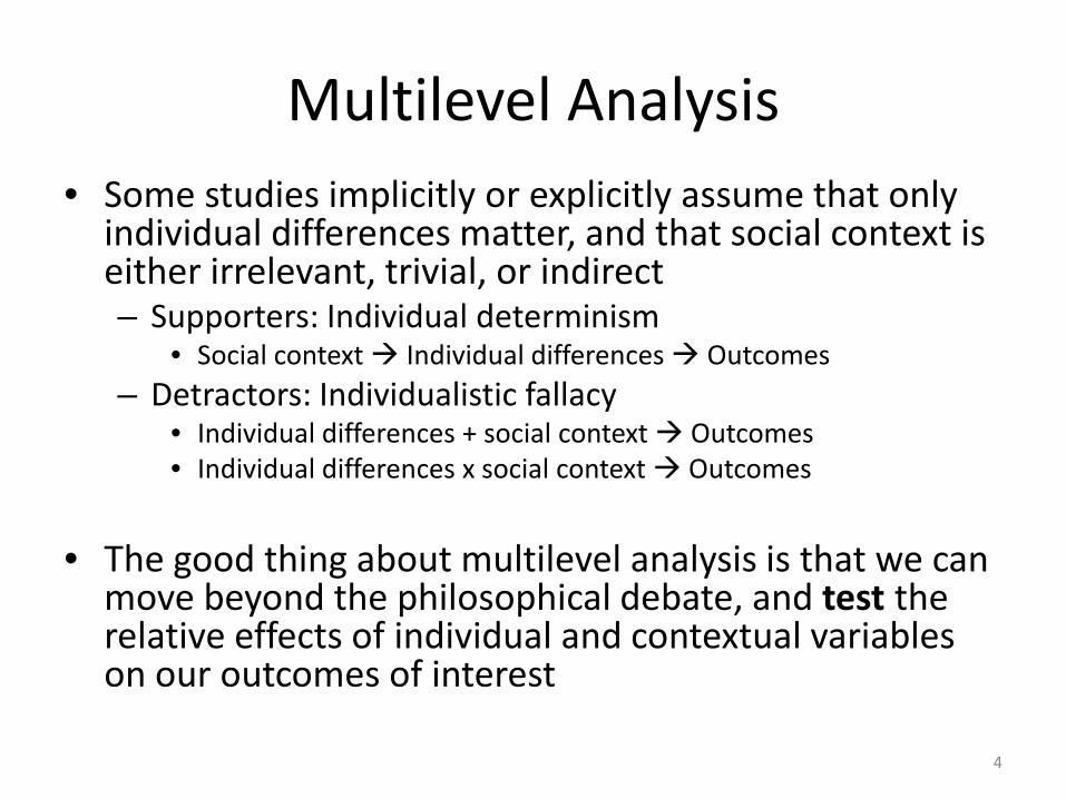
Multilevel Analysis • Some studies implicitly or explicitly assume that only
individual differences matter, and that social context is either irrelevant, trivial, or indirect – Supporters: Individual determinism
• Social context Individual differences Outcomes – Detractors: Individualistic fallacy
• Individual differences + social context Outcomes • Individual differences x social context Outcomes
• The good thing about multilevel analysis is that we can
move beyond the philosophical debate, and test the relative effects of individual and contextual variables on our outcomes of interest
4
Multilevel Analysis
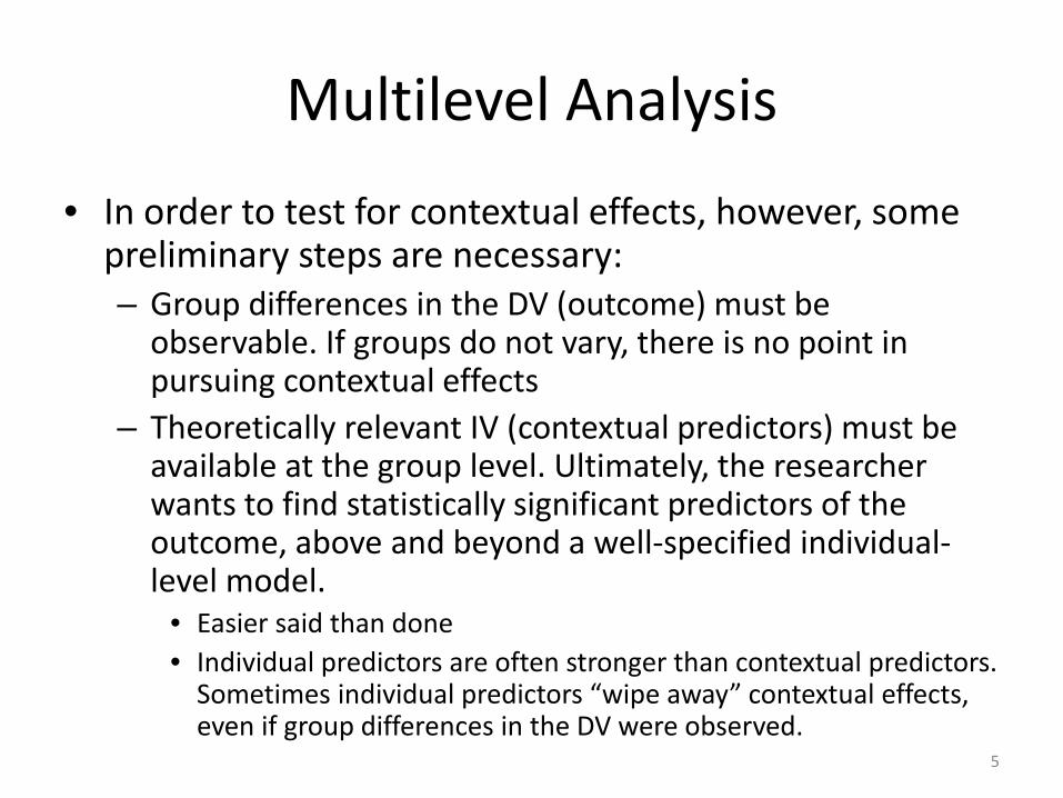
• In order to test for contextual effects, however, some preliminary steps are necessary: – Group differences in the DV (outcome) must be
observable. If groups do not vary, there is no point in pursuing contextual effects
– Theoretically relevant IV (contextual predictors) must be available at the group level. Ultimately, the researcher wants to find statistically significant predictors of the outcome, above and beyond a well-specified individual-level model.
• Easier said than done • Individual predictors are often stronger than contextual predictors.
Sometimes individual predictors “wipe away” contextual effects, even if group differences in the DV were observed.
5
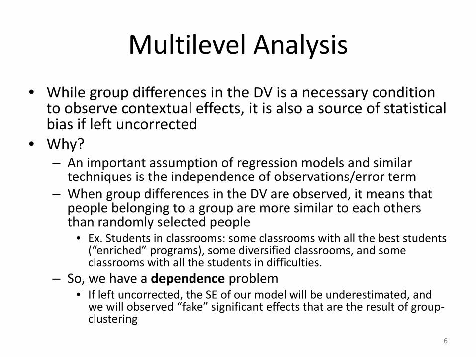
Multilevel Analysis • While group differences in the DV is a necessary condition
to observe contextual effects, it is also a source of statistical bias if left uncorrected
• Why? – An important assumption of regression models and similar
techniques is the independence of observations/error term – When group differences in the DV are observed, it means that
people belonging to a group are more similar to each others than randomly selected people
• Ex. Students in classrooms: some classrooms with all the best students (“enriched” programs), some diversified classrooms, and some classrooms with all the students in difficulties.
– So, we have a dependence problem • If left uncorrected, the SE of our model will be underestimated, and
we will observed “fake” significant effects that are the result of group-clustering
6
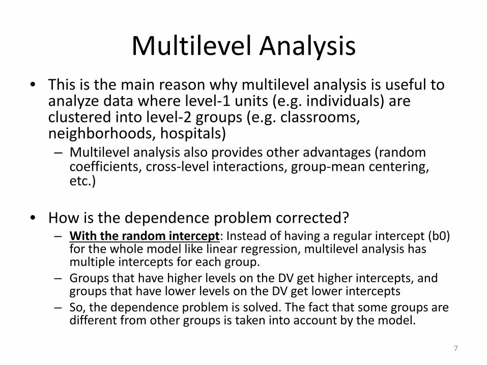
Multilevel Analysis • This is the main reason why multilevel analysis is useful to
analyze data where level-1 units (e.g. individuals) are clustered into level-2 groups (e.g. classrooms, neighborhoods, hospitals) – Multilevel analysis also provides other advantages (random
coefficients, cross-level interactions, group-mean centering, etc.)
• How is the dependence problem corrected? – With the random intercept: Instead of having a regular intercept (b0)
for the whole model like linear regression, multilevel analysis has multiple intercepts for each group.
– Groups that have higher levels on the DV get higher intercepts, and groups that have lower levels on the DV get lower intercepts
– So, the dependence problem is solved. The fact that some groups are different from other groups is taken into account by the model.
7
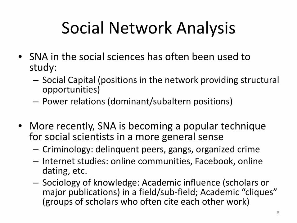
Social Network Analysis • SNA in the social sciences has often been used to
study: – Social Capital (positions in the network providing structural
opportunities) – Power relations (dominant/subaltern positions)
• More recently, SNA is becoming a popular technique
for social scientists in a more general sense – Criminology: delinquent peers, gangs, organized crime – Internet studies: online communities, Facebook, online
dating, etc. – Sociology of knowledge: Academic influence (scholars or
major publications) in a field/sub-field; Academic “cliques” (groups of scholars who often cite each other work)
8
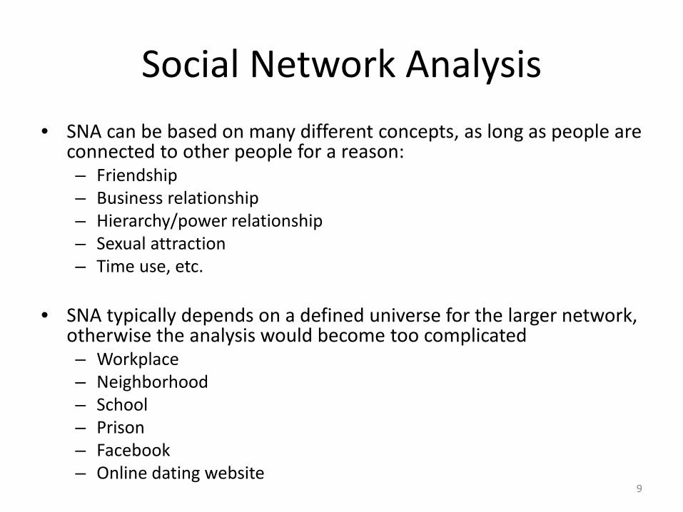
Social Network Analysis • SNA can be based on many different concepts, as long as people are
connected to other people for a reason: – Friendship – Business relationship – Hierarchy/power relationship – Sexual attraction – Time use, etc.
• SNA typically depends on a defined universe for the larger network,
otherwise the analysis would become too complicated – Workplace – Neighborhood – School – Prison – Facebook – Online dating website
9
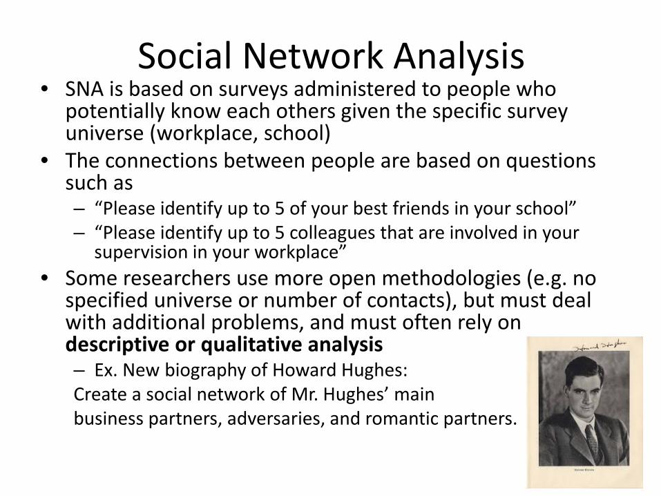
Social Network Analysis • SNA is based on surveys administered to people who
potentially know each others given the specific survey universe (workplace, school)
• The connections between people are based on questions such as – “Please identify up to 5 of your best friends in your school” – “Please identify up to 5 colleagues that are involved in your
supervision in your workplace” • Some researchers use more open methodologies (e.g. no
specified universe or number of contacts), but must deal with additional problems, and must often rely on descriptive or qualitative analysis – Ex. New biography of Howard Hughes: Create a social network of Mr. Hughes’ main business partners, adversaries, and romantic partners.
10
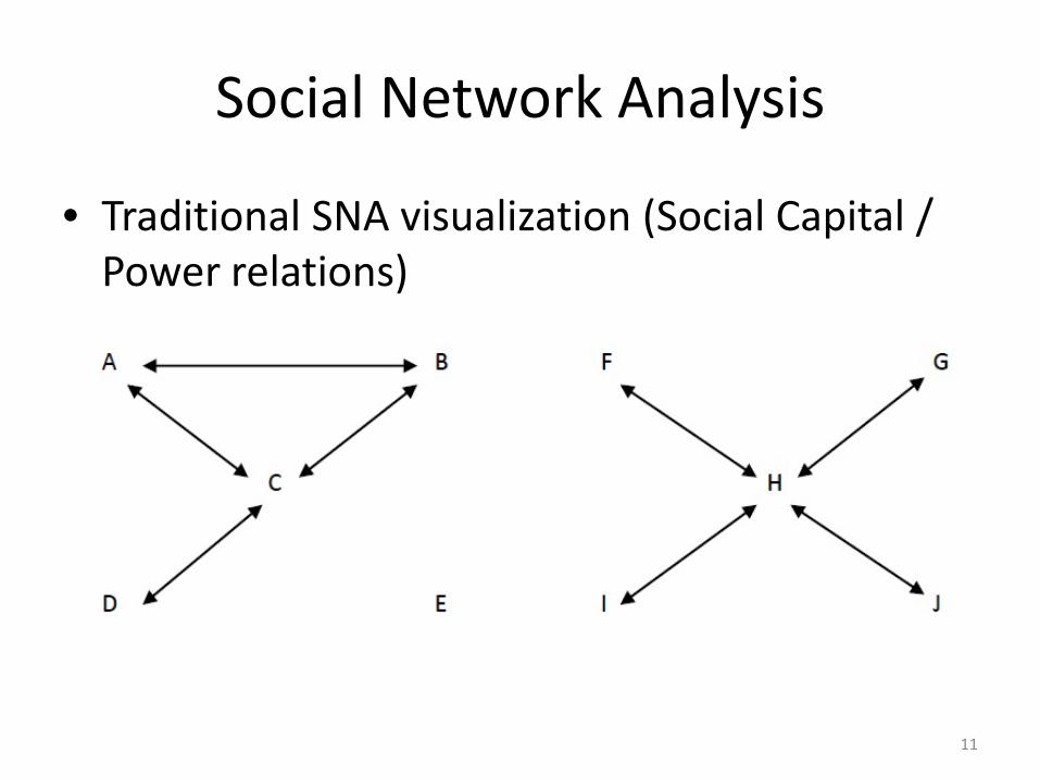
Social Network Analysis
• Traditional SNA visualization (Social Capital / Power relations)
11
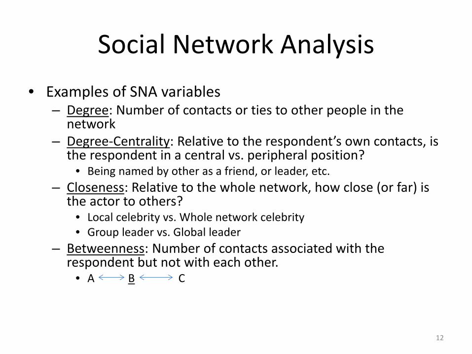
Social Network Analysis • Examples of SNA variables
– Degree: Number of contacts or ties to other people in the network
– Degree-Centrality: Relative to the respondent’s own contacts, is the respondent in a central vs. peripheral position?
• Being named by other as a friend, or leader, etc. – Closeness: Relative to the whole network, how close (or far) is
the actor to others? • Local celebrity vs. Whole network celebrity • Group leader vs. Global leader
– Betweenness: Number of contacts associated with the respondent but not with each other.
• A B C
12
Social Network Analysis
• New applications of SNA: – Examine complex connections between large
groups of people (see picture in a few slides), and empirically isolate coherent smaller groups (peers, gangs, workplace teams, etc.) from the larger network.
• Groups, and individuals in these groups, can be compared in follow-up analyses
• In other words, the SNA is a first step in a larger analysis
13
Making the Connection • Fact 1: We have one technique that allows us to group
people together based on different conceptualization of networks (e.g. friendship, business relationship) and to create empirical variables from the networks
• Fact 2: We have another technique that allows us to elegantly analyze data involving smaller units clustered into larger units, control clustering biases, and estimate contextual effects above and beyond individual effects
• Logical connection: Social network analysis can generate datasets in which individuals (smaller units) are grouped into their network clusters (larger units), ready to be analyzed with multilevel models
14
Making the Connection • Variance components (individual variance within groups
vs. variance between groups) in multilevel analysis is of special interest in the social network context: – It can be interpreted as a measure of sociability of behaviors – The larger the between groups variance, the more social is the
behavior (vs. individual behavior) – At one extreme, if 100% variance is within group, and 0%
between groups, the behavior is purely individual... Groups don't matter!
– At the other extreme, if 0% variance is within group, and 100% between groups, the behavior is purely social... Individuals behave in perfect conformity with their own group and all the variation is between groups!
– In reality, there is often a division of the variance within and between groups, but different behaviors can be compared in regard to their level of sociability 15
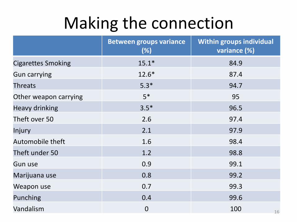
Making the connection Between groups variance
(%) Within groups individual
variance (%)
Cigarettes Smoking 15.1* 84.9 Gun carrying 12.6* 87.4 Threats 5.3* 94.7 Other weapon carrying 5* 95 Heavy drinking 3.5* 96.5 Theft over 50 2.6 97.4 Injury 2.1 97.9 Automobile theft 1.6 98.4 Theft under 50 1.2 98.8 Gun use 0.9 99.1 Marijuana use 0.8 99.2 Weapon use 0.7 99.3 Punching 0.4 99.6 Vandalism 0 100 16
Empirical example: Delinquency and Peer Networks
• It is well known that delinquents often have delinquent friends.
• However, this pattern may reflect: – Peer influences: peer group-level factors increasing
the risk of delinquency of respondents – Self selection: individual variations in risk factors for
delinquency and seeking out like-minded peers – No peer group effects
– Hybrid model: peer group factors interacting with individual risk factors for delinquency – Peer group influences conditional on individual differences
17
Empirical example: Delinquency and Peer Networks
• Data: 550 high school students, who could nominate up to 5 close friends – Data collected in 2006, from a mid-size high
school in Kentucky • The survey allowed respondents to nominate
friends outside of schools, but they mostly nominated friends from school
• Analysis is based on friends from school, since friends must also take the survey
18
Empirical example: Delinquency and Peer Networks
• Part 1: Social Network Analysis • Main concept: friendship (peer groups) • SNA typically combines visualization techniques
(mapping) with statistical tests (e.g. network cohesion, actor centrality, network subgroups)
• Based on both visualization and statistical tests, the researcher must make reasonable decisions about the final number of network clusters.
• UCINET software was used for the current study
19
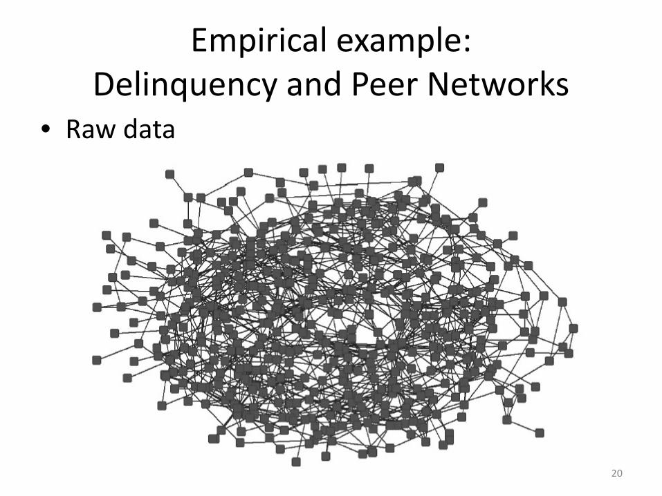
Empirical example: Delinquency and Peer Networks
• Raw data
20
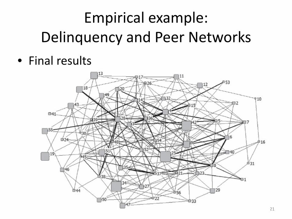
Empirical example: Delinquency and Peer Networks
• Final results
21
Empirical example: Delinquency and Peer Networks
• Two previous image taken from: Swartz et al. (2012) Patterns of victimization between and within peer clusters in a high school social network. Violence and Victims 27: 710-729.
• The same data are used in the current study • Based on the final results of the SNA, 56 peer groups
(a.k.a. network clusters) were measured • Final sample of respondents for the multilevel analysis
is 514 – 17 loners were deleted – Lost a few more respondents because they did not provide
answers for key DVs
22
Empirical example: Delinquency and Peer Networks
• Part 2: Multilevel Analysis • Level 1: Delinquency variables and individual risk
factors • Level 2: Group-average for the peer clusters on
two key predictors: (1) peer-group average level of low self control; (2) peer-group average level of deviant attitudes
• For simplicity sake, preliminary results are estimated with the linear HLM regression for this example – Replicated them with the Poisson HLM regression and
the patterns did not change 23
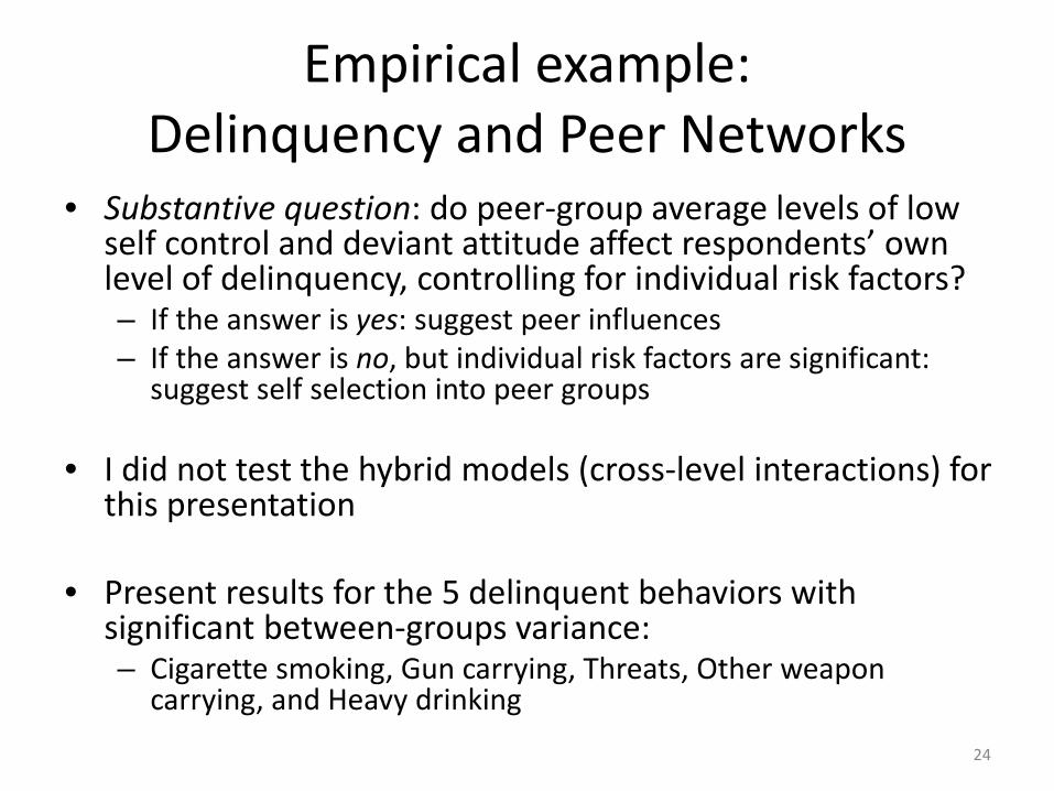
Empirical example: Delinquency and Peer Networks
• Substantive question: do peer-group average levels of low self control and deviant attitude affect respondents’ own level of delinquency, controlling for individual risk factors? – If the answer is yes: suggest peer influences – If the answer is no, but individual risk factors are significant:
suggest self selection into peer groups
• I did not test the hybrid models (cross-level interactions) for this presentation
• Present results for the 5 delinquent behaviors with significant between-groups variance: – Cigarette smoking, Gun carrying, Threats, Other weapon
carrying, and Heavy drinking 24
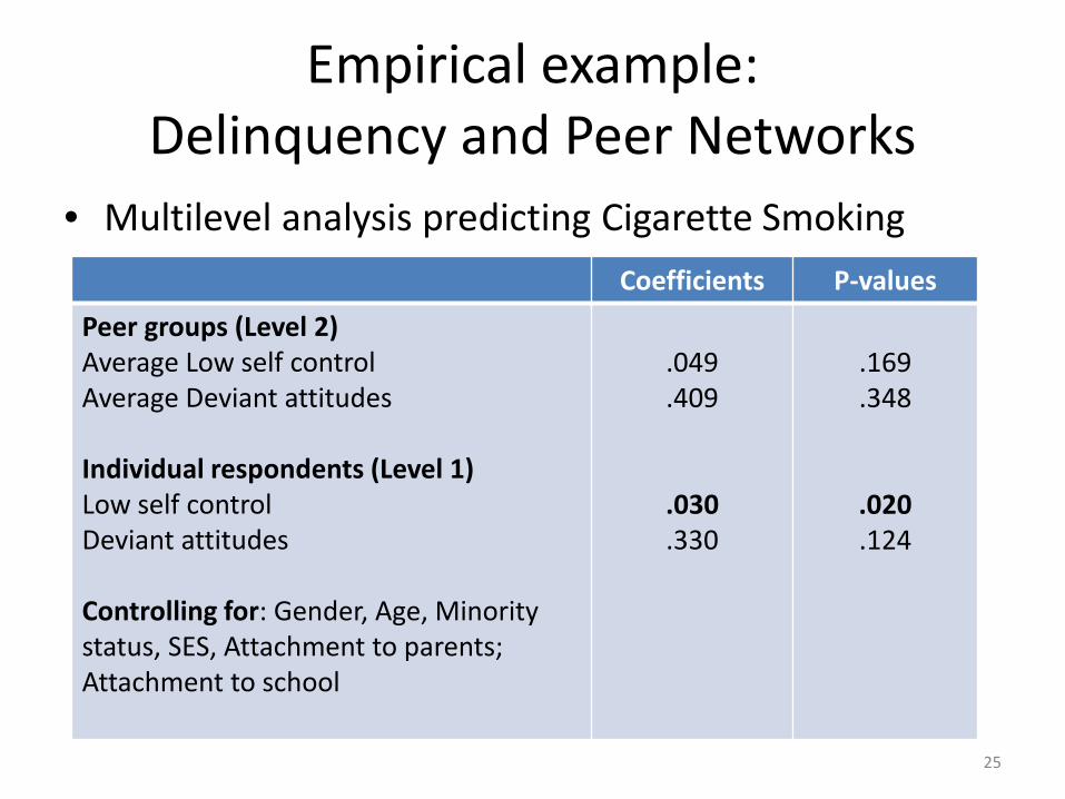
Empirical example: Delinquency and Peer Networks
• Multilevel analysis predicting Cigarette Smoking
25
Coefficients P-values Peer groups (Level 2) Average Low self control Average Deviant attitudes Individual respondents (Level 1) Low self control Deviant attitudes Controlling for: Gender, Age, Minority status, SES, Attachment to parents; Attachment to school
.049 .409
.030
.330
.169 .348
.020
.124
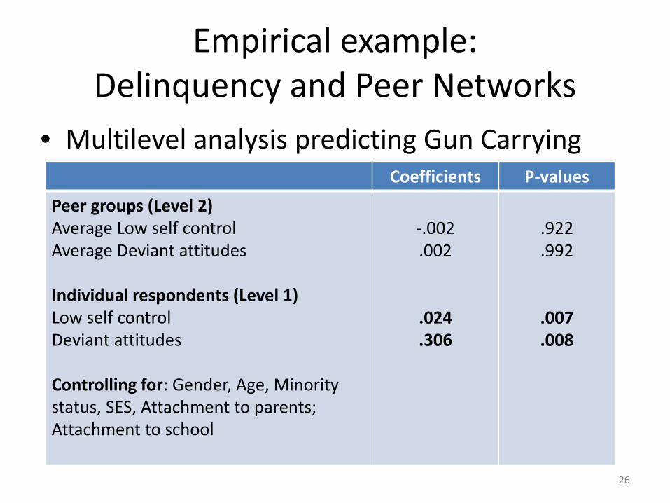
Empirical example: Delinquency and Peer Networks
• Multilevel analysis predicting Gun Carrying
26
Coefficients P-values Peer groups (Level 2) Average Low self control Average Deviant attitudes Individual respondents (Level 1) Low self control Deviant attitudes Controlling for: Gender, Age, Minority status, SES, Attachment to parents; Attachment to school
-.002 .002
.024
.306
.922 .992
.007
.008
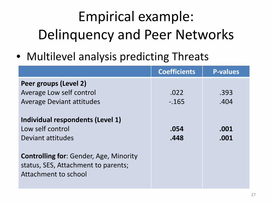
Empirical example: Delinquency and Peer Networks
• Multilevel analysis predicting Threats
27
Coefficients P-values Peer groups (Level 2) Average Low self control Average Deviant attitudes Individual respondents (Level 1) Low self control Deviant attitudes Controlling for: Gender, Age, Minority status, SES, Attachment to parents; Attachment to school
.022 -.165
.054
.448
.393 .404
.001
.001
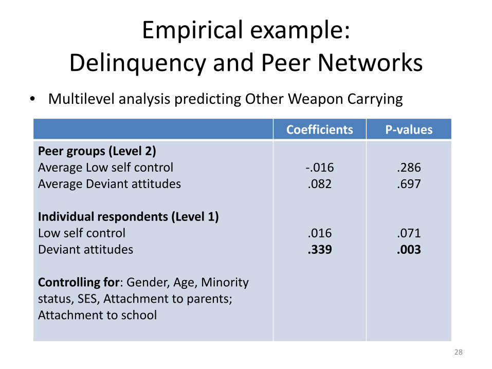
Empirical example: Delinquency and Peer Networks
• Multilevel analysis predicting Other Weapon Carrying
28
Coefficients P-values Peer groups (Level 2) Average Low self control Average Deviant attitudes Individual respondents (Level 1) Low self control Deviant attitudes Controlling for: Gender, Age, Minority status, SES, Attachment to parents; Attachment to school
-.016 .082
.016
.339
.286 .697
.071
.003
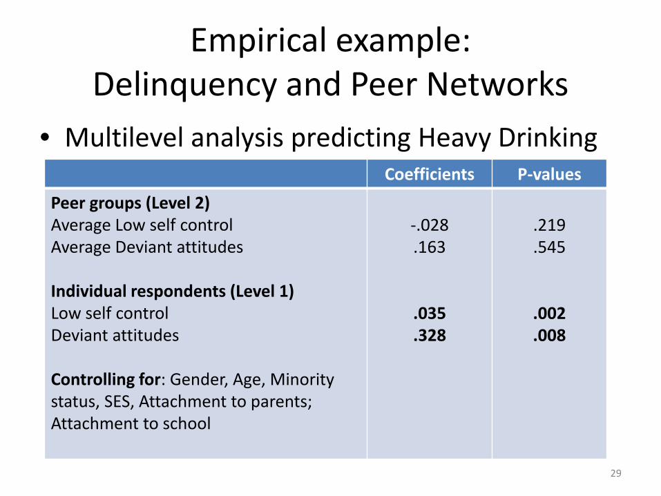
Empirical example: Delinquency and Peer Networks
• Multilevel analysis predicting Heavy Drinking
29
Coefficients P-values Peer groups (Level 2) Average Low self control Average Deviant attitudes Individual respondents (Level 1) Low self control Deviant attitudes Controlling for: Gender, Age, Minority status, SES, Attachment to parents; Attachment to school
-.028 .163
.035
.328
.219 .545
.002
.008
Empirical example: Delinquency and Peer Networks
• Preliminary Discussion: – Results from variance components show that some
delinquent behaviors are more social (smoking, gun carrying), while other delinquent behaviors are more individual (vandalism, punching someone)
– Results do not show support for group-level peer influences in term of average levels of low self control or deviant attitudes
– Rather, they show fairly consistent support for the effects of individual levels of low self control and deviant attitudes
– Thus, preliminary results suggest that self selection may play a greater role than peer influences in explaining why delinquents tend to have delinquent friends
30
Limitations • Early decisions in the survey design and data collection
have important implications at later stages – Researchers must think in terms of sampling of
respondents but also sampling universe for the network – Results will vary based on sampling universe for the
network: people at work, people in your neighborhood, people at school, people on Facebook, etc.
– The number of possible contacts: identify your 3 best friends from work (vs. 5, vs. 10)
– Wording: • “Identify your best friends” vs. “Identify people you trust the
most” • “Identify people with the most power in your workplace” vs.
“Identify people who directly exercise power over you on a daily basis in your workplace”
31
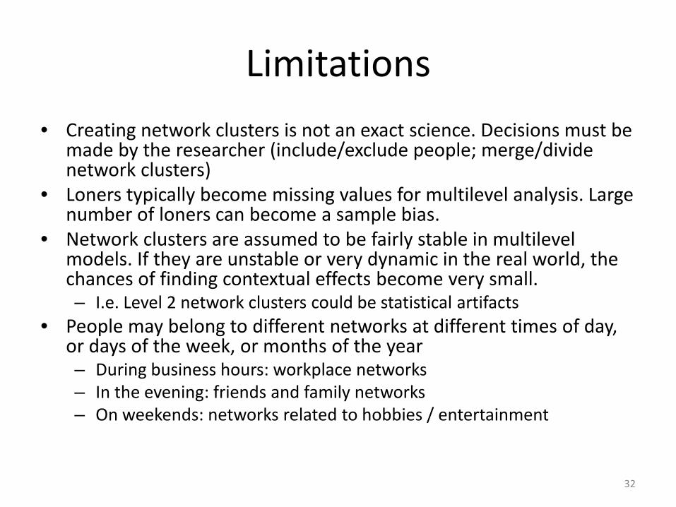
Limitations • Creating network clusters is not an exact science. Decisions must be
made by the researcher (include/exclude people; merge/divide network clusters)
• Loners typically become missing values for multilevel analysis. Large number of loners can become a sample bias.
• Network clusters are assumed to be fairly stable in multilevel models. If they are unstable or very dynamic in the real world, the chances of finding contextual effects become very small. – I.e. Level 2 network clusters could be statistical artifacts
• People may belong to different networks at different times of day, or days of the week, or months of the year – During business hours: workplace networks – In the evening: friends and family networks – On weekends: networks related to hobbies / entertainment
32
Limitations
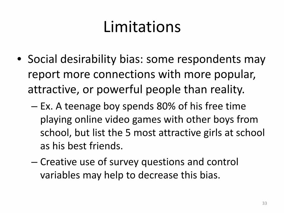
• Social desirability bias: some respondents may report more connections with more popular, attractive, or powerful people than reality. – Ex. A teenage boy spends 80% of his free time
playing online video games with other boys from school, but list the 5 most attractive girls at school as his best friends.
– Creative use of survey questions and control variables may help to decrease this bias.
33
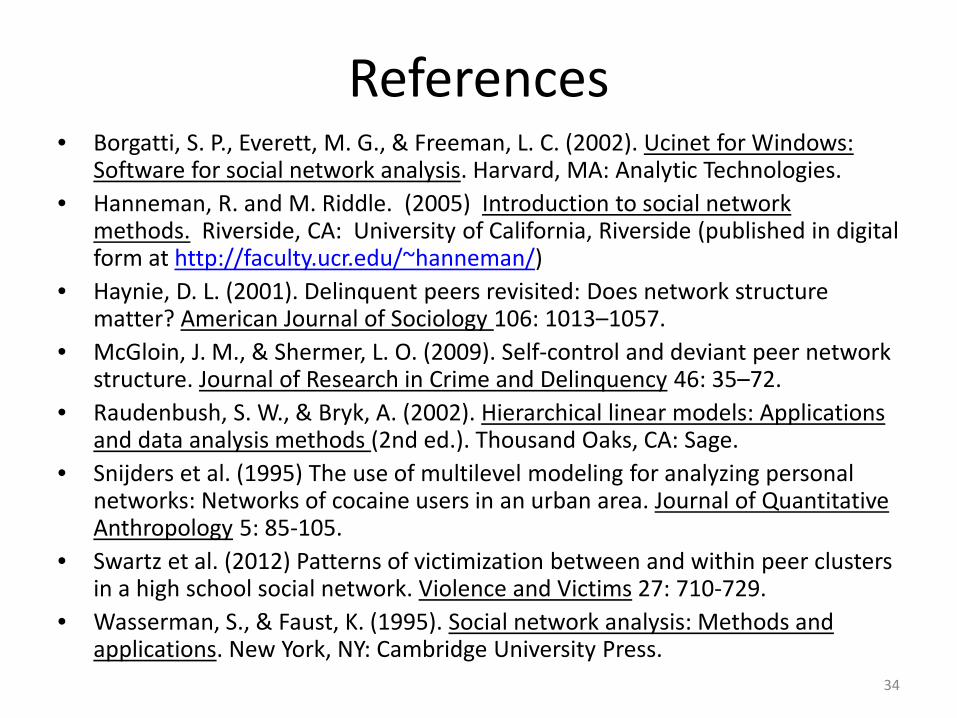
References • Borgatti, S. P., Everett, M. G., & Freeman, L. C. (2002). Ucinet for Windows:
Software for social network analysis. Harvard, MA: Analytic Technologies. • Hanneman, R. and M. Riddle. (2005) Introduction to social network
methods. Riverside, CA: University of California, Riverside (published in digital form at http://faculty.ucr.edu/~hanneman/)
• Haynie, D. L. (2001). Delinquent peers revisited: Does network structure matter? American Journal of Sociology 106: 1013–1057.
• McGloin, J. M., & Shermer, L. O. (2009). Self-control and deviant peer network structure. Journal of Research in Crime and Delinquency 46: 35–72.
• Raudenbush, S. W., & Bryk, A. (2002). Hierarchical linear models: Applications and data analysis methods (2nd ed.). Thousand Oaks, CA: Sage.
• Snijders et al. (1995) The use of multilevel modeling for analyzing personal networks: Networks of cocaine users in an urban area. Journal of Quantitative Anthropology 5: 85-105.
• Swartz et al. (2012) Patterns of victimization between and within peer clusters in a high school social network. Violence and Victims 27: 710-729.
• Wasserman, S., & Faust, K. (1995). Social network analysis: Methods and applications. New York, NY: Cambridge University Press.
34