Embed Size (px)
Citation preview

Multilevel Monte Carlo methods
Mike Giles
Mathematical Institute, University of Oxford
SIAM Conference on Uncertainty Quantification
April 5-8, 2016
Acknowledgements to many collaborators:
Frances Kuo, Ian Sloan (UNSW), Des Higham, Xuerong Mao (Strathclyde),Rob Scheichl, Aretha Teckentrup (Bath), Andrew Cliffe (Nottingham),Ruth Baker, Ben Hambly, Christoph Reisinger, Endre Suli (Oxford),
Klaus Ritter (Kaiserslautern), Lukas Szpruch (Edinburgh),
Jaime Peraire, Ferran Vidal-Codina (MIT), . . .
Mike Giles (Oxford) Multilevel Monte Carlo 1 / 39

Objectives
In presenting the multilevel Monte Carlo method, I hope to emphasise:
the simplicity of the idea
its flexibility – it’s not prescriptive, more an approach
there are lots of people working on a variety of applications
In doing this, I will focus on ideas rather than lots of numerical results.
Mike Giles (Oxford) Multilevel Monte Carlo 2 / 39

Monte Carlo method
In stochastic models, we often have
ω −→ S −→ P
random input intermediate variables scalar output
The Monte Carlo estimate for E[P ] is an average of N independentsamples ω(n):
Y = N−1N∑
n=1
P(ω(n)).
This is unbiased, E[Y ]=E[P ], and the Central Limit Theorem proves thatas N → ∞ the error becomes Normally distributed with variance N−1
V[P ].
Mike Giles (Oxford) Multilevel Monte Carlo 3 / 39

Monte Carlo method
In many cases, this is modified to
ω −→ S −→ P
random input intermediate variables scalar output
where S , P are approximations to S ,P , in which case the MC estimate
Y = N−1N∑
n=1
P(ω(n))
is biased, and the Mean Square Error is
E[ (Y −E[P ])2] = N−1V[P] +
(E[P]− E[P ]
)2
Greater accuracy requires larger N and smaller weak error E[P ]−E[P ].
Mike Giles (Oxford) Multilevel Monte Carlo 4 / 39
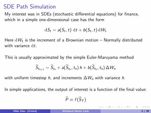
SDE Path Simulation
My interest was in SDEs (stochastic differential equations) for finance,which in a simple one-dimensional case has the form
dSt = a(St , t) dt + b(St , t)dWt
Here dWt is the increment of a Brownian motion – Normally distributedwith variance dt.
This is usually approximated by the simple Euler-Maruyama method
Stn+1 = Stn + a(Stn , tn) h + b(Stn , tn)∆Wn
with uniform timestep h, and increments ∆Wn with variance h.
In simple applications, the output of interest is a function of the final value:
P ≡ f (ST )
Mike Giles (Oxford) Multilevel Monte Carlo 5 / 39

SDE Path Simulation
Geometric Brownian Motion: dSt = r St dt + σ St dWt
t0 0.5 1 1.5 2
S
0.5
1
1.5
coarse pathfine path
Mike Giles (Oxford) Multilevel Monte Carlo 6 / 39

SDE Path Simulation
Two kinds of discretisation error:
Weak error:E[P ]− E[P ] = O(h)
Strong error: (E
[sup[0,T ]
(St−St
)2])1/2
= O(h1/2)
For reasons which will become clear, I prefer to use the Milsteindiscretisation for which the weak and strong errors are both O(h).
Mike Giles (Oxford) Multilevel Monte Carlo 7 / 39

SDE Path Simulation
The Mean Square Error is
N−1V[P] +
(E[P ]− E[P ]
)2≈ a N−1 + b h2
If we want this to be ε2, then we need
N = O(ε−2), h = O(ε)
so the total computational cost is O(ε−3).
To improve this cost we need to
reduce N – variance reduction or Quasi-Monte Carlo methods
reduce the cost of each path (on average) – MLMC
Mike Giles (Oxford) Multilevel Monte Carlo 8 / 39

Two-level Monte Carlo
If we want to estimate E[P1] but it is much cheaper to simulate P0 ≈ P1,then since
E[P1] = E[P0] + E[P1−P0]
we can use the estimator
N−10
N0∑
n=1
P(0,n)0 + N−1
1
N1∑
n=1
(P(1,n)1 − P
(1,n)0
)
Benefit: if P1−P0 is small, its variance will be small, so won’t need manysamples to accurately estimate E[P1−P0], so cost will be reduced greatly.
Mike Giles (Oxford) Multilevel Monte Carlo 9 / 39

Multilevel Monte Carlo
Natural generalisation: given a sequence P0, P1, . . . , PL
E[PL] = E[P0] +
L∑
ℓ=1
E[Pℓ−Pℓ−1]
we can use the estimator
N−10
N0∑
n=1
P(0,n)0 +
L∑
ℓ=1
{N−1ℓ
Nℓ∑
n=1
(P(ℓ,n)ℓ − P
(ℓ,n)ℓ−1
)}
with independent estimation for each level of correction
Mike Giles (Oxford) Multilevel Monte Carlo 10 / 39

Multilevel Monte Carlo
If we define
C0,V0 to be cost and variance of P0
Cℓ,Vℓ to be cost and variance of Pℓ−Pℓ−1
then the total cost isL∑
ℓ=0
Nℓ Cℓ and the variance isL∑
ℓ=0
N−1ℓ Vℓ.
Using a Lagrange multiplier µ2 to minimise the cost for a fixed variance
∂
∂Nℓ
L∑
k=0
(Nk Ck + µ2N−1
kVk
)= 0
givesNℓ = µ
√Vℓ/Cℓ =⇒ Nℓ Cℓ = µ
√Vℓ Cℓ
Mike Giles (Oxford) Multilevel Monte Carlo 11 / 39

Multilevel Monte Carlo
Setting the total variance equal to ε2 gives
µ = ε−2
(L∑
ℓ=0
√Vℓ Cℓ
)
and hence, the total cost is
L∑
ℓ=0
Nℓ Cℓ = ε−2
(L∑
ℓ=0
√VℓCℓ
)2
in contrast to the standard cost which is approximately ε−2 V0 CL.
The MLMC cost savings are therefore approximately:
VL/V0, if√VℓCℓ increases with level
C0/CL, if√VℓCℓ decreases with level
Mike Giles (Oxford) Multilevel Monte Carlo 12 / 39

Multilevel Path SimulationWith SDEs, level ℓ corresponds to approximation using Mℓ timesteps,giving approximate payoff Pℓ at cost Cℓ = O(h−1
ℓ ).
Simplest estimator for E[Pℓ−Pℓ−1] for ℓ>0 is
Yℓ = N−1ℓ
Nℓ∑
n=1
(P(n)ℓ −P
(n)ℓ−1
)
using same driving Brownian path for both levels.
Analysis gives MSE =
L∑
ℓ=0
N−1ℓ Vℓ +
(E[PL]−E[P ]
)2
To make RMS error less than ε
choose Nℓ ∝√
Vℓ/Cℓ so total variance is less than 12 ε
2
choose L so that(E[PL]−E[P ]
)2< 1
2 ε2
Mike Giles (Oxford) Multilevel Monte Carlo 13 / 39

Multilevel Path Simulation
For Lipschitz payoff functions P ≡ f (ST ), we have
Vℓ ≡ V
[Pℓ−Pℓ−1
]≤ E
[(Pℓ−Pℓ−1)
2]
≤ K 2E
[(ST ,ℓ−ST ,ℓ−1)
2]
=
{O(hℓ), Euler-Maruyama
O(h2ℓ ), Milstein
and hence
Vℓ Cℓ =
{O(1), Euler-Maruyama
O(hℓ), Milstein
Mike Giles (Oxford) Multilevel Monte Carlo 14 / 39

MLMC Theorem
(Slight generalisation of version in 2008 Operations Research paper)
If there exist independent estimators Yℓ based on Nℓ Monte Carlo samples,each costing Cℓ, and positive constants α, β, γ, c1, c2, c3 such thatα≥ 1
2 min(β, γ) and
i)∣∣∣E[Pℓ−P ]
∣∣∣ ≤ c1 2−α ℓ
ii) E[Yℓ] =
E[P0], ℓ = 0
E[Pℓ−Pℓ−1], ℓ > 0
iii) V[Yℓ] ≤ c2 N−1ℓ 2−β ℓ
iv) E[Cℓ] ≤ c3 2γ ℓ
Mike Giles (Oxford) Multilevel Monte Carlo 15 / 39

MLMC Theorem
then there exists a positive constant c4 such that for any ε<1 there existL and Nℓ for which the multilevel estimator
Y =
L∑
ℓ=0
Yℓ,
has a mean-square-error with bound E
[(Y − E[P ]
)2]< ε2
with an expected computational cost C with bound
C ≤
c4 ε−2, β > γ,
c4 ε−2(log ε)2, β = γ,
c4 ε−2−(γ−β)/α, 0 < β < γ.
Mike Giles (Oxford) Multilevel Monte Carlo 16 / 39

MLMC Theorem
Two observations of optimality:
MC simulation needs O(ε−2) samples to achieve RMS accuracy ε.When β > γ, the cost is optimal — O(1) cost per sample on average.
(Would need multilevel QMC to further reduce costs)
When β < γ, another interesting case is when β = 2α, which
corresponds to E[Yℓ] and√
E[Y 2ℓ ] being of the same order as ℓ → ∞.
In this case, the total cost is O(ε−γ/α), which is the cost of a singlesample on the finest level — again optimal.
Mike Giles (Oxford) Multilevel Monte Carlo 17 / 39

MLMC generalisation
The theorem is for scalar outputs P , but it can be generalised tomulti-dimensional (or infinite-dimensional) outputs with
i)∥∥∥E[Pℓ−P ]
∥∥∥ ≤ c1 2−α ℓ
ii) E[Yℓ] =
E[P0], ℓ = 0
E[Pℓ−Pℓ−1], ℓ > 0
iii) V[Yℓ] ≡ E
[∥∥∥Yℓ − E[Yℓ]∥∥∥2]≤ c2 N
−1ℓ 2−β ℓ
Original multilevel research by Heinrich in 1999 did this for parametricintegration, estimating g(λ) ≡ E[f (x , λ)] for a finite-dimensional r.v. x .
Mike Giles (Oxford) Multilevel Monte Carlo 18 / 39

MLMC work on SDEs
Milstein discretisation for path-dependent options – G (2008)
numerical analysis – G, Higham, Mao (2009), Avikainen (2009),G, Debrabant, Roßler (2012)
financial sensitivities (“Greeks”) – Burgos (2011)
jump-diffusion models – Xia (2011)
Levy processes – Dereich (2010), Marxen (2010), Dereich &Heidenreich (2011), Xia (2013), Kyprianou (2014)
American options – Belomestny & Schoenmakers (2011)
Milstein in higher dimensions without Levy areas – G, Szpruch (2014)
adaptive timesteps – Hoel, von Schwerin, Szepessy, Tempone (2012),G, Lester, Whittle (2014)
Mike Giles (Oxford) Multilevel Monte Carlo 19 / 39

SPDEs
quite natural application, with better cost savings than SDEsdue to higher dimensionality
range of applications◮ Graubner & Ritter (Darmstadt) – parabolic◮ G, Reisinger (Oxford) – parabolic◮ Cliffe, G, Scheichl, Teckentrup (Bath/Nottingham) – elliptic◮ Barth, Jenny, Lang, Meyer, Mishra, Muller, Schwab, Sukys, Zollinger
(ETH Zurich) – elliptic, parabolic, hyperbolic◮ Harbrecht, Peters (Basel) – elliptic◮ Efendiev (Texas A&M) – numerical homogenization◮ Vidal-Codina, G, Peraire (MIT) – reduced basis approximation
Mike Giles (Oxford) Multilevel Monte Carlo 20 / 39

Engineering Uncertainty Quantification
Simplest possible example:
3D elliptic PDE, with uncertain boundary data
grid spacing proportional to 2−ℓ on level ℓ
cost is O(2+3ℓ), if using an efficient multigrid solver
2nd order accuracy means that
Pℓ(ω)− P(ω) ≈ c(ω) 2−2ℓ
=⇒ Pℓ−1(ω)− Pℓ(ω) ≈ 3 c(ω) 2−2ℓ
hence, α=2, β=4, γ=3
cost is O(ε−2) to obtain ε RMS accuracy
this compares to O(ε−3/2) cost for one sample on finest level,so O(ε−7/2) for standard Monte Carlo
Mike Giles (Oxford) Multilevel Monte Carlo 21 / 39

PDEs with Uncertainty
I worked with Rob Scheichl (Bath) and Andrew Cliffe (Nottingham)on multilevel Monte Carlo for the modelling of oil reservoirs andgroundwater contamination in nuclear waste repositories.
Here we have an elliptic SPDE coming from Darcy’s law:
∇·(κ(x)∇p
)= 0
where the permeability κ(x) is uncertain, and log κ(x) is often modelled asbeing Normally distributed with a spatial covariance such as
cov(log κ(x1), log κ(x2)) = σ2 exp(−‖x1−x2‖/λ)
Mike Giles (Oxford) Multilevel Monte Carlo 22 / 39

Elliptic SPDE
A typical realisation of κ for λ = 0.01, σ = 1.
Mike Giles (Oxford) Multilevel Monte Carlo 23 / 39
Elliptic SPDE
Samples of log k are provided by a Karhunen-Loeve expansion:
log k(x, ω) =
∞∑
n=0
√θn ξn(ω) fn(x),
where θn, fn are eigenvalues / eigenfunctions of the correlation function:
∫R(x, y) fn(y) dy = θn fn(x)
and ξn(ω) are standard Normal random variables.
Numerical experiments truncate the expansion.
(Latest 2D/3D work uses a more efficient FFT construction based on acirculant embedding.)
Mike Giles (Oxford) Multilevel Monte Carlo 24 / 39

Elliptic SPDE
Decay of 1D eigenvalues
100
101
102
103
10−6
10−4
10−2
100
n
eige
nval
ue
λ=0.01λ=0.1λ=1
When λ = 1, can use a low-dimensional polynomial chaos approach,but it’s impractical for smaller λ.
Mike Giles (Oxford) Multilevel Monte Carlo 25 / 39

Elliptic SPDE
Discretisation:
cell-centred finite volume discretisation on a uniform grid – for roughcoefficients we need to make grid spacing very small on finest grid
each level of refinement has twice as many grid points in eachdirection
early numerical experiments used a direct solver for simplicity,but later work in 3D uses an efficient AMG multigrid solver witha cost roughly proportional to the total number of grid points
later work also considers other finite element discretisations– doesn’t make any substantial difference to MLMC treatment
Mike Giles (Oxford) Multilevel Monte Carlo 26 / 39

2D Results
Boundary conditions for unit square [0, 1]2:– fixed pressure: p(0, x2)=1, p(1, x2)=0– Neumann b.c.: ∂p/∂x2(x1, 0)=∂p/∂x2(x1, 1)=0
Output quantity – mass flux: −∫
k∂p
∂x1dx2
Correlation length: λ = 0.2
Coarsest grid: h = 1/8 (comparable to λ)
Finest grid: h = 1/128
Karhunen-Loeve truncation: mKL = 4000
Cost taken to be proportional to number of nodes
Mike Giles (Oxford) Multilevel Monte Carlo 27 / 39

2D Results
0 1 2 3 4−12
−10
−8
−6
−4
−2
0
2
level l
log 2 v
aria
nce
Pl
Pl− P
l−1
0 1 2 3 4−12
−10
−8
−6
−4
−2
0
2
level l
log 2 |m
ean|
Pl
Pl− P
l−1
V[Pℓ−Pℓ−1] ∼ h2ℓ E[Pℓ−Pℓ−1] ∼ h2ℓ
Mike Giles (Oxford) Multilevel Monte Carlo 28 / 39

2D Results
0 1 2 3 410
2
103
104
105
106
107
108
level l
Nl
10−3
10−2
100
101
102
accuracy ε
ε2 Cos
t
Std MCMLMC
ε=0.0005ε=0.001ε=0.002ε=0.005ε=0.01
Mike Giles (Oxford) Multilevel Monte Carlo 29 / 39

Complexity analysis
Relating things back to the MLMC theorem:
E[Pℓ−P ] ∼ 2−2ℓ =⇒ α = 2
Vℓ ∼ 2−2ℓ =⇒ β = 2
Cℓ ∼ 2dℓ =⇒ γ = d (dimension of PDE)
To achieve r.m.s. accuracy ε requires finest level grid spacing h ∼ ε1/2
and hence we get the following complexity:
dim MC MLMC
1 ε−2.5 ε−2
2 ε−3 ε−2(log ε)2
3 ε−3.5 ε−2.5
Mike Giles (Oxford) Multilevel Monte Carlo 30 / 39

Non-geometric multilevel
Almost all applications of multilevel in the literature so far use a geometricsequence of levels, refining the timestep (or the spatial discretisation forPDEs) by a constant factor when going from level ℓ to level ℓ+ 1.
Coming from a multigrid background, this is very natural, but it is NOTa requirement of the multilevel Monte Carlo approach.
All MLMC needs is a sequence of levels with
increasing accuracy
increasing cost
increasingly small difference between outputs on successive levels
Mike Giles (Oxford) Multilevel Monte Carlo 31 / 39

Reduced Basis PDE approximationVidal-Codina, Nguyen, G, Peraire (2014) take a fine FE discretisation:
A(ω) u = f (ω)
and use a reduced basis approximation
u ≈K∑
k=1
vkuk
to obtain a low-dimensional reduced system
Ar (ω) v = fr (ω)
larger K =⇒ greater accuracy at greater cost
in multilevel treatment, Kℓ varies with level
brute force optimisation determines the optimal number of levels,and reduced basis size on each level
Mike Giles (Oxford) Multilevel Monte Carlo 32 / 39

Other MLMC applications
parametric integration, integral equations (Heinrich)
multilevel QMC (Dick, G, Kuo, Scheichl, Schwab, Sloan)
stochastic chemical reactions (Anderson & Higham, Tempone)
mixed precision computation on FPGAs (Korn, Ritter, Wehn)
MLMC for MCMC (Scheichl, Schwab, Stuart, Teckentrup)
Coulomb collisions in plasma (Caflisch)
nested simulation (Haji-Ali & Tempone, Hambly & Reisinger)
invariant distribution of contractive Markov process (Glynn & Rhee)
invariant distribution of contractive SDEs (G, Lester & Whittle)
Mike Giles (Oxford) Multilevel Monte Carlo 33 / 39

Three MLMC extensions
unbiased estimation – Rhee & Glynn (2015)◮ randomly selects the level for each sample◮ no bias, and finite expected cost and variance if β > γ
Richardson-Romberg extrapolation – Lemaire & Pages (2013)◮ reduces the weak error, and hence the number of levels required◮ particularly helpful when β < γ
Multi-Index Monte Carlo – Haji-Ali, Nobile, Tempone (2015)◮ important extension to MLMC approach, combining MLMC with
sparse grid methods
Mike Giles (Oxford) Multilevel Monte Carlo 34 / 39

Multi-Index Monte Carlo
Standard “1D” MLMC truncates the telescoping sum
E[P ] =∞∑
ℓ=0
E[∆Pℓ]
where ∆Pℓ ≡ Pℓ − Pℓ−1, with P−1≡0.
In “2D”, MIMC truncates the telescoping sum
E[P ] =
∞∑
ℓ1=0
∞∑
ℓ2=0
E[∆Pℓ1,ℓ2 ]
where ∆Pℓ1,ℓ2 ≡ (Pℓ1,ℓ2 − Pℓ1−1,ℓ2)− (Pℓ1,ℓ2−1 − Pℓ1−1,ℓ2−1)
Different aspects of the discretisation vary in each “dimension” – for a 2DPDE, could use grid spacing 2−ℓ1 in direction 1, 2−ℓ2 in direction 2
Mike Giles (Oxford) Multilevel Monte Carlo 35 / 39

Multi-Index Monte Carlo
✲
✻
ℓ1
ℓ2
❅❅❅❅❅❅❅❅❅❅❅❅
❡ ❡
❡ ❡
four evaluations forcross-difference ∆P(3,2)
r r r r r r
r r r r r
r r r r
r r r
r r
r
MIMC truncates the summation in a way which minimises the cost toachieve a target MSE – quite similar to sparse grids.
Can achieve O(ε−2) complexity for a wider range of SPDE and otherapplications than plain MLMC.
Mike Giles (Oxford) Multilevel Monte Carlo 36 / 39

Conclusions
multilevel idea is very simple; key question is how to apply it innew situations, and perform the numerical analysis
discontinuous output functions can cause problems, but there isa lot of experience now in coping with this
there are also “tricks” which can be used in situations with poorstrong convergence
being used for an increasingly wide range of applications;biggest computational savings when coarsest (reasonable)approximation is much cheaper than finest
currently, getting at least 100× savings for SPDEs and stochasticchemical reaction simulations
Mike Giles (Oxford) Multilevel Monte Carlo 37 / 39

References
Webpages for my research papers and talks:
people.maths.ox.ac.uk/gilesm/mlmc.html
people.maths.ox.ac.uk/gilesm/slides.html
Webpage for new 70-page Acta Numerica review and MATLAB test codes:
people.maths.ox.ac.uk/gilesm/acta/
– contains references to almost all MLMC research
Mike Giles (Oxford) Multilevel Monte Carlo 38 / 39

MLMC CommunityWebpage: people.maths.ox.ac.uk/gilesm/mlmc community.htmlAbo Academi (Avikainen) – numerical analysisBasel (Harbrecht) – elliptic SPDEs, sparse gridsBath (Kyprianou, Scheichl, Shardlow, Yates) – elliptic SPDEs, MCMC, Levy-driven SDEs, stochastic chemical modellingChalmers (Lang) – SPDEsDuisburg (Belomestny) – Bermudan and American optionsEdinburgh (Davie, Szpruch) – SDEs, numerical analysisEPFL (Abdulle) – stiff SDEs and SPDEsETH Zurich (Jenny, Jentzen, Schwab) – SPDEs, multilevel QMCFrankfurt (Gerstner, Kloeden) – numerical analysis, fractional Brownian motionFraunhofer ITWM (Iliev) – SPDEs in engineeringHong Kong (Chen) – Brownian meanders, nested simulation in financeIIT Chicago (Hickernell) – SDEs, infinite-dimensional integration, complexity analysisKaiserslautern (Heinrich, Korn, Ritter) – finance, SDEs, parametric integration, complexity analysisKAUST (Tempone) – adaptive time-stepping, stochastic chemical modellingKiel (Gnewuch) – randomized multilevel QMCLPMA (Frikha, Lemaire, Pages) – numerical analysis, multilevel extrapolation, finance applicationsMannheim (Neuenkirch) – numerical analysis, fractional Brownian motionMIT (Peraire) – uncertainty quantification, SPDEsMunich (Hutzenthaler) – numerical analysisOxford (Baker, Giles, Hambly, Reisinger, Suli) – SDEs, SPDEs, nested simulation, numerical analysis, finance applications,
stochastic chemical reactions, long-chain moleculesPassau (Muller-Gronbach) – infinite-dimensional integration, complexity analysisStanford (Glynn) – numerical analysis, randomized multilevelStrathclyde (Higham, Mao) – numerical analysis, exit times, stochastic chemical modellingStuttgart (Barth) – SPDEsTexas A&M (Efendiev) – SPDEs in engineeringUCLA (Caflisch) – Coulomb collisions in physicsUNSW (Dick, Kuo, Sloan) – multilevel QMCWarwick (Stuart, Teckentrup) – MCMC for SPDEsWIAS (Friz, Schoenmakers) – rough paths, fractional Brownian motion, Bermudan optionsWisconsin (Anderson) – numerical analysis, stochastic chemical modelling
WWU (Dereich) – Levy-driven SDEsMike Giles (Oxford) Multilevel Monte Carlo 39 / 39