Embed Size (px)
Citation preview

Multilevel Potential Outcome Models for Causal Inference in Jury Research
by
David Lovis-McMahon
A Dissertation Presented in Partial Fulfillment
of the Requirements for the Degree
Doctor of Philosophy
Approved July 2015 by the
Graduate Supervisory Committee:
Michael Saks, Co-Chair
Nicholas Schweitzer, Co-Chair
Jessica Salerno
David Mackinnon
ARIZONA STATE UNIVERSITY
August 2015
i
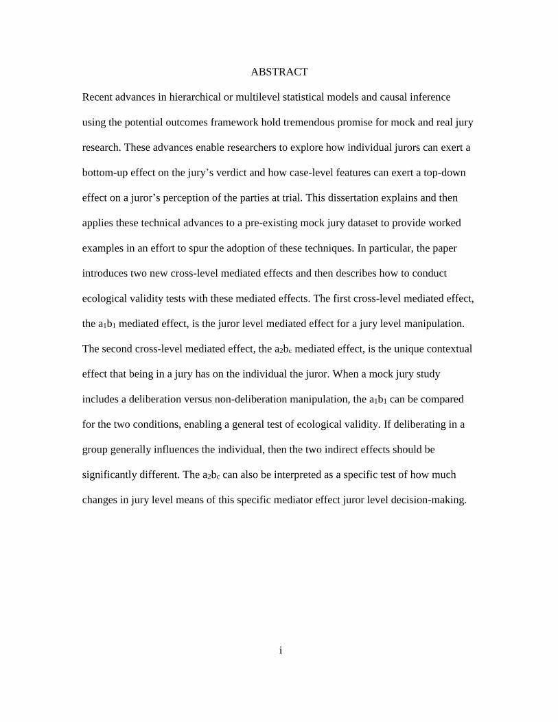
ABSTRACT
Recent advances in hierarchical or multilevel statistical models and causal inference
using the potential outcomes framework hold tremendous promise for mock and real jury
research. These advances enable researchers to explore how individual jurors can exert a
bottom-up effect on the jury’s verdict and how case-level features can exert a top-down
effect on a juror’s perception of the parties at trial. This dissertation explains and then
applies these technical advances to a pre-existing mock jury dataset to provide worked
examples in an effort to spur the adoption of these techniques. In particular, the paper
introduces two new cross-level mediated effects and then describes how to conduct
ecological validity tests with these mediated effects. The first cross-level mediated effect,
the a1b1 mediated effect, is the juror level mediated effect for a jury level manipulation.
The second cross-level mediated effect, the a2bc mediated effect, is the unique contextual
effect that being in a jury has on the individual the juror. When a mock jury study
includes a deliberation versus non-deliberation manipulation, the a1b1 can be compared
for the two conditions, enabling a general test of ecological validity. If deliberating in a
group generally influences the individual, then the two indirect effects should be
significantly different. The a2bc can also be interpreted as a specific test of how much
changes in jury level means of this specific mediator effect juror level decision-making.

ii
DEDICATION
Amy Louise Carpenter – I think I left it better than I found it.
Stephen Mark Carpenter – You may not have been my father, but I’ll always be grateful
you chose to be my dad.
Douglas Charles McMahon – I wish I could have gotten to know you.

iii
ACKNOWLEDGMENTS
There are more people to whom I am grateful than there is space here to
acknowledge.
To Brett Barker, I think that extremely awkward grade change you made for me
in AP Psychology paid off. Thank you for believing in me when so much of my life was
a mess my junior year.
To my committee members, Nick Schweitzer, Michael Saks, Jessica Salerno, and
David MacKinnon, thank you for support and enthusiasm for this project. I know you're
feedback has helped make this better than what I could have done alone.
I would like to give a special thanks to Nick Schweitzer for taking me on as my
primary advisor. Thank you for helping me navigate being the first student in the joint
psychology and law program.
I would also like to thank David MacKinnon for inviting me to be a part of his
Research in Prevention lab. It was a great and unexpected opportunity.
I've been fortunate enough to be surrounded by amazing and talented individuals
over the years – Andrew White, Elizabeth Osborne, Ashley Votruba, Keelah Williams,
Gabrielle Filip-Crawford, Alex Danvers, Sarah Herrmann, and Jessica Bodford. To my
cohort, Andrew and Beth, there was nobody I'd rather have decorating the office than you
two. To my fellow social psychology and law cohort, Ashley and Keelah, you're
accomplishments are awe inspiring and I'm proud to be member of this very elite group.
To Gabrielle and Alex, thank you for being my close friends. To Sarah and Jessica, you
are wonderful and thoughtful researchers who will do great things.

iv
Lastly, I want to thank my dear friends and family who helped temper the
madness of the 2,895 days it took me to finish this program – Ian Tingen, Crista Alvey,
Crow Tomkus, and Andreea Danielescu. You've made me a better person.
v
TABLE OF CONTENTS
Page
LIST OF TABLES ................................................................................................................. vii
LIST OF FIGURES .............................................................................................................. viii
CHAPTER
1 INTRODUCTION ................. ..................................................................................... 1
Mediation Analysis .................................................................................... 2
Multilevel Models ...................................................................................... 5
Searle Dataset Background ........................................................................ 8
Project’s Goals ......................................................................................... 11
2 POTENTIAL OUTCOMES MODEL ..................................................................... 16
Counterfactually Defined Causal Effects ................................................ 17
Mediated Effects ...................................................................................... 19
Real Data Example ................................................................................... 24
3 MULTILEVEL MODELS ............ ............................................................................ 28
Sources of Variation, Contextual Effects, and Centering ....................... 28
Real Data Example ................................................................................... 30
4 INTEGRATED MLM MEDIATION MODELS .................................................... 38
Revisiting Contextual Effects .................................................................. 38
The Role of Centering in Defining Cross-Level Mediated Effects ........ 40
Cross-Level Mediators ............................................................................. 41
vi
5 DATA ANALYSIS AND RESULTS ...................................................................... 43
Overview of Mediated Effects ................................................................. 44
Ecological Validity Tests ......................................................................... 44
Summary and Synthesis of Mediated Effects ......................................... 45
6 IMPLICATIONS AND EXTENSIONS .................................................................. 47
Implications for the Design of Mock Jury Research ............................... 47
Non-normal Mediators and Dependent Variables .................................. 49
Longitudinal Mediation ........................................................................... 50
Implications of the Verdict-Confidence DV ........................................... 51
Conclusion ................................................................................................ 51
REFERENCES....... ............................................................................................................... 52
APPENDIX
A CRITIQUE OF VERDICT-CONFIDENCE COMPOSITE ................................. 56
B MPLUS SYNTAX .................................................................................................. 69
B ICC, DESIGN EFFECTS, AND EFFECTIVE N .................................................. 75

vii
LIST OF TABLES
Table Page
1. Descriptive Statistics for the Mediator ................................................................. 10
2. Descriptive Statistics for the Dependent Variable ................................................ 11
3. Comparison of Traditional versus Counterfactually Defined Effects .................. 26
4. Traditional 2-2-2 Models Analyzed With vs Without Respect to Clustering ..... 35
5. Comparison of Mediated Effects .......................................................................... 43

viii
LIST OF FIGURES
Figure Page
1. Common Path Diagram for Single Mediator Model ........................................... 3
2. Conceptual Diagram of Proposed Multilevel Mediator Model .......................... 7
3. Conceptual Diagram of the Single Leve, Single Mediator Model ................... 19
4. Path Diagram for Single Mediator, Single Level Model .................................. 25
5. Coefficient Plot of the Estimated Causal Effects from Table 3 ........................ 26
6. Within Cluster versus Between Cluster Sources of Variability ........................ 31
7. The Effect of Grand versus Group Mean Centering ......................................... 33
8. Conceptual Model of Traditional 2-2-2 Analysis ............................................ 34
9. Coefficient Plot of Estimated MLM Mediated Effects in Table 4 ................... 35
10. Conceptual Diagram of the Two Possible Cross-Level Indirect Effects ....... 42
11. Path Model for Counterfactually Defined Effects ......................................... 42
12. Coefficient Plot Summarzing the Mediated Effects in Table 5 ..................... 43

1
CHAPTER 1
INTRODUCTION
Since its inception, modern jury researchers have faced the daunting task of
studying a phenomenon that has two simultaneous levels of analysis. Understanding the
American jury necessitates an analytical framework capable of modeling the individual
juror, the collective jury, and the interaction between the two. Researchers studying jury
decision-making have long theorized about the interplay between juror and jury in
reaching the final jury verdict; however, much of this research investigates the juror-level
and the jury-level components in isolation (Bornstein & Greene, 2011; Devine,
Buddenbaum, Houp, Studebaker, & Stolle, 2009; Devine, Clayton, Dunford, Seying, &
Pryce, 2001). Although the story model and DISCUSS have proven to be successful in
their respective domains, this isolationism persists despite the long-theorized role of the
interplay between juror and jury in reaching the final jury verdict (Devine et al., 2001;
Devine, 2012; Kalven & Zeisel, 1971; Pennington & Hastie, 1993, 1994; Stasser, 1988).
The present project aims to develop a statistical model capable of simultaneously
addressing research questions involving both how individual jurors can exert a bottom-up
effect on the jury’s verdict, and how case-level features can exert a top-down effect on a
juror’s perception of the parties at trial (Devine et al., 2001; Imai, Keele, & Tingley,
2010; Imai, King, & Stuart, 2008; Imai & van Dyk, 2004; Krull & MacKinnon, 1999;
Krull & MacKinnon, 2001; MacKinnon, 2012; Pituch & Stapleton, 2012; Preacher,
Zyphur, & Zhang, 2010).
This dissertation presents a synthesis of the modern statistical methods for causal
inference via the potential outcomes model with multilevel models. For example, using a

2
multilevel framework it is possible to identify the unique effect that the evidence
presented at trial to the jury has on a juror’s initial damage award. Although knowing this
is useful, it is an incomplete description of the psychological processes that connects the
evidence to the damage award. To fully identify the mechanisms driving the juror and
jury decision-making processes requires extending the statistical models to incorporate
both juror- and jury-level variables as potential mediating mechanisms.
Mediation Analysis
The goal of the method proposed here is to further substantive researchers’ ability
to ask and obtain answers to the research questions regarding jury decision-making. Take
the following example: How does the strength or quality of evidence presented by a
plaintiff influence the outcome of a trial? Moreover, do perceptions of the plaintiff’s
personality mediate that link? Substantive researchers have a variety of options and
methods to answer this question, but these methods only work if the juror- and jury-level
analyses are treated independently and are not allowed to influence one another, which
they undoubtedly do.
Research into methods for evaluating causal mechanisms has grown rapidly since
the causal steps approach to testing mediation was first outlined (Baron & Kenny, 1986;
Judd & Kenny, 1981). Each advance from the product-of-coefficients to the newest
counterfactually defined effects has brought with it new ways of studying causal
mechanisms. At their core, however, each of these approaches simply identify different
ways to decompose the total effect of an Indpendent Variable (IV) on a Dependent
Variable (DV) into a remaining direct effect and an indirect effect that passes through a
proposed mediating third variable.

3
Traditionally Defined Mediated Effects
Initially presented in Kenny and Judd (1981) and Baron and Kenny (1986), the
causal steps approach defines mediation indirectly as the difference between the total
effect estimated in one regression and the direct effect in a second regression (see figure
1). That is, one first regresses the DV on the IV; this is the total effect or c path. Second,
the DV is this regressed on the IV plus the mediator, the regression coefficient for the IV
is now the partial effect controlling for the mediator and is referred to as the direct effect
or c’ path. Third, the difference between the total effect (c path) and the direct effect (c’
path) is tested. If that difference is significant, then there is evidence of partial mediation.
If the direct effect (c’) is now non-significant, then there is evidence of complete
mediation.
Figure 1. Common path diagram for single mediator model.
The causal steps approach has an intuitive appeal, but it also has several
limitations. First, defining mediation as the difference-in-coefficients limits the research
question to single mediator designs. If more than one mediator were included, it would be
impossible to assess which of the two mediators is the cause for significant difference.
Thus, more complex multiple mediator designs cannot be readily assessed using the

4
causal steps approach. Second, because of the strong assumption of normality embedded
in the causal steps, the total and direct effects used to define mediation are inconsistent
when applied to cases in which the mediator or the outcome are non-normal—for
example, a binary mediator or binary outcome (Mackinnon & Dwyer, 1993; MacKinnon,
2008). In essence, the causal steps approach defines a recipe for inferring mediation, but
does not provide a principled definition.
Although the product-of-coefficients approach emerged after the causal steps
approach was outlined, it has a deeper history in the path analysis and structural equation
modeling (SEM) traditions. Here, the use of simultaneous regressions enables the direct
estimation of the indirect effect as the product of the a and b paths. By directly defining
the indirect effect, it is possible to test multiple mediators simultaneously. By being
contained within the SEM tradition, mediated effects can be tested using advances in the
SEM framework—such as latent variable measurement models, modern missing data
techniques, multiple mediators, and for certain kinds of multilevel models. However, as
with the causal steps approach, there is a strong assumption that all of the variables are
linearly related, and in the presence of non-linear effects it is not clear how to define
indirect effects or direct effects (Muthén & Asparouhov, 2014).
Counterfactually Defined Mediated Effects
The most recent work in defining mediated effects utilizes the potential outcomes
model, which is relatively new to psychology but has seen decades of active use in other
social sciences (Imai, Keele, & Tingley, 2010; MacKinnon & Pirlott, 2014; Morgan &
Winship, 2014). The potential outcomes model is a deeply philosophical and
5
mathematical model that uses logic to provide “counterfactual” causal definitions, which
can then be used to derive “causal” estimators in statistical models.
As discussed in Morgan and Winship (2014), the combination of the potential
outcomes model with the research on directed acyclical graphs can be thought of as a
successor to the path analysis and SEM traditions. From this point of view, the potential
outcomes model generalizes the traditional SEM method beyond a strictly linear
framework. This resolves one of the major difficulties of testing for mediation in jury
research. More importantly, the potential outcomes model provides a principled
definition of a cause via a counterfactual, which is why the direct and indirect effects
estimated are sometimes called counterfactually defined effects. As discussed below, this
enables the model to provide additional or alternative definitions for mediated effects that
would not be possible using the causal steps or the SEM tradition.
As noted earlier, these three approaches are unified by the basic decomposition of
the total effect into the sum of the direct and indirect effects. As such, in the single
mediator model, when the variables are all linearly related and there is no XM
interaction, the three approaches produce the exact same evidence for mediation because
they produce identical direct and indirect estimates.
Multilevel Models
Traditionally Defined Mediated Effects
If the researcher is interested in individual jurors, chapter 2 details both traditional
SEM and counterfactual methods to assess what the mediated effect (ab) might be for the
individual juror (see figure 1). These methods work so long as the individual jurors have
not been assigned to a jury (i.e., the methods assume there is no clustering). Critically,

6
any inferences from this kind of experiment applied to a jury run the risk of committing
the atomistic fallacy: one cannot draw inferences about group behavior from the behavior
of individual units.
If instead the researcher is interested in juries, chapter 3 details traditional
multilevel methods for assessing what the mediated effect (a2b2) might be for juries.
These methods work so long as all of the variables of interest exist at the jury-level.
Similarly, any inferences from this kind of experiment run the risk of committing the
ecological fallacy: one cannot draw inferences about individual behavior from the
behavior of groups.
Before the recent mainstream adoption of multilevel models, jury researchers
were often forced to analyze the levels separately, focusing on either the juror- or the
jury-level relationships. Disaggregating the data to focus solely on the juror-level
relationships assumes that all observations are independent—which, when violated,
underestimates standard errors, producing alpha inflation. Aggregating the data to focus
solely on the jury-level relationships induces numerous interpretation challenges and
invites committing the ecological fallacy. Critically, both methods for separating the data
analysis share the same flaw: they assume the relation between variables is identical
within clusters as well as between clusters.
Thus, even if a researcher were to conduct an experiment where individuals were
randomly assigned to either deliberate in juries versus not deliberate, the mediated effects
using the methods discussed in chapters 2 and 3 are incommensurate because they
estimate fundamentally different quantities. It is tempting to think that the difference in
the mediated effects might be attributable to the effect of being on a jury, but because the
7
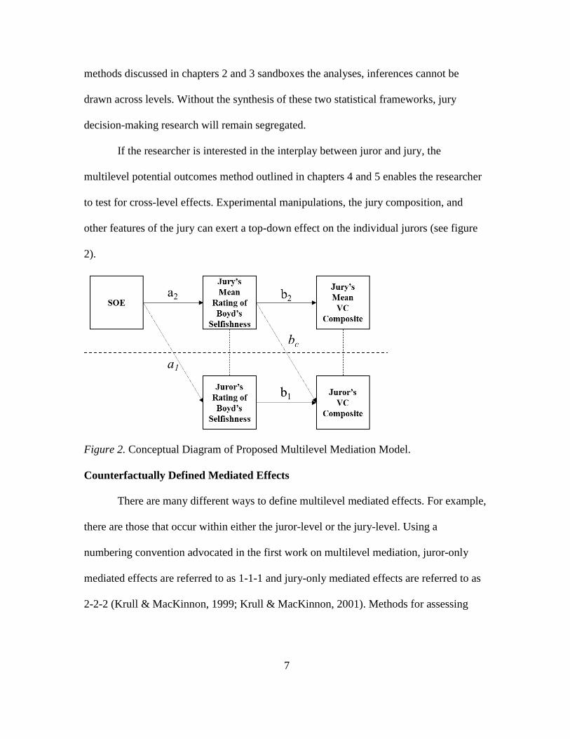
methods discussed in chapters 2 and 3 sandboxes the analyses, inferences cannot be
drawn across levels. Without the synthesis of these two statistical frameworks, jury
decision-making research will remain segregated.
If the researcher is interested in the interplay between juror and jury, the
multilevel potential outcomes method outlined in chapters 4 and 5 enables the researcher
to test for cross-level effects. Experimental manipulations, the jury composition, and
other features of the jury can exert a top-down effect on the individual jurors (see figure
2).
Figure 2. Conceptual Diagram of Proposed Multilevel Mediation Model.
Counterfactually Defined Mediated Effects
There are many different ways to define multilevel mediated effects. For example,
there are those that occur within either the juror-level or the jury-level. Using a
numbering convention advocated in the first work on multilevel mediation, juror-only
mediated effects are referred to as 1-1-1 and jury-only mediated effects are referred to as
2-2-2 (Krull & MacKinnon, 1999; Krull & MacKinnon, 2001). Methods for assessing

8
mediation in these contexts have already been developed and applied in the psychology
literature; I will conduct both of those kinds of analyses in chapters 2 and 3, respectively.
What is exciting about this project is that it is one of the first to use advances in
multilevel mediation spurred by the potential outcomes model to define new cross-level
mediated effects. In particular, in chapters 4 and 5 I will describe and apply two new
cross-level mediated effects. The first occurs when a jury-level predictor or experimental
manipulation is thought to influence a juror-level mediator that in turn influences a juror-
level DV, referred to as a 2-1-1 mediated effect. The second occurs when a jury-level
predictor or experimental manipulation is thought to influence a jury-level mediator that
in turn influences a juror-level DV, referred to as a 2-2-1 mediated effect.
Although there are other possible cross-level mediated effects, testing for these
two effects follows naturally in jury research studies where juries are assigned to
experimental manipulations. It is fruitful to have a tool that enables researchers to, for
example, test theories about whether the race of the defendant at trial influences the
ultimate verdict by either 1) changing the thought processes of the individual juror; 2)
changing the immediate context the juror is situated in; or 3) changing both
simultaneously.
Searle Dataset Background
Since the Searle mock jury dataset (Diamond, Saks, & Landsman, 1998;
Landsman, Diamond, Dimitropoulos, & Saks, 1998) will be used throughout the
remaining chapters to illustrate important concepts, a discussion of the dataset is
warranted before chapter 5. Originally collected in the early 1990’s, the extensive dataset
is one of the most complex mock jury studies conducted. The study’s original goals were
9
in part to determine the effects of evidence strength and jury bifurcation on jury verdicts
and damage awards in a civil trial. Participants were jury-eligible adults recruited from
Cook County, Illinois, with the goal of matching the Cook County jury pool. Although
1,042 participants were recruited, 21 were excluded for giving inconsistent responses
between verdict and damage awards. Of the original 1,042 participants, 720 were
assigned to deliberate in six-person juries, while the remaining 322 served as individual
non-deliberating jurors.
Mock jurors were asked to provide responses at three different stages. In the first
stage, prior to viewing the trial video, participants were asked to complete a demographic
and background information questionnaire (e.g., education level and prior smoking
history). In addition, participants were asked to provide answers to questions involving
attitudes towards business, lawsuits, and the legal system. In the second stage, after
watching the video of the trial, participants were asked to provide pre-deliberation
verdicts on liability, compensatory damages, punitive liability, punitive damages, and a
confidence score for both liability and punitive liability verdicts. In the last stage, after
deliberation, participants were asked a series of comprehension questions along with
questions intended to probe the jurors’ reasoning about their individualized pre-
deliberation verdict.
Variables of Interest
Several decisions have been made to help simplify the data analysis while
maintaining its instructional value. First, while there were several experimental
manipulations, for the purposes of this dissertation I will use only the evidence strength
manipulation as a level-2 or jury-level independent variable. The evidence strength

10
manipulation has two levels, consisting of weak versus moderate evidence strength. In
the weak evidence condition, there is ample evidence that the plaintiff’s smoking habit of
two-and-a-half packs a day is responsible for his lung cancer. In contrast, the moderate
evidence condition provides stronger evidence that the plaintiff’s on-the-job exposure to
the fictive carcinogen Beryllico is responsible for his lung cancer.
The participants’ rating of the perceived selfishness of the plaintiff Mr. Boyd was
selected as the mediator. Participants were given a series of words to rate the plaintiff on,
and this question was scored on a 1 (“selfish”) to 7 (“concerned for others”) point scale
(see table 1 for descriptive statistics).
Table 1
Descriptive Statistics for the Mediator
Deliberators Non-Deliberators
Juror-level Jury-level
Mean - 4.587 4.600
Std. Dev 1.315 0.399 1.512
ICC 0.084 -
Design Effect 1.410 -
Effective N 500.177 -
Lastly, for the dependent variable, a Verdict-Confidence composite was formed
by taking the juror’s verdict as coded -1 (defendant) and 1 (plaintiff) multiplied by their
self-rated confidence in that verdict on a 1 (“not at all confident”) to 7 (“completely
confident”) scale. Thus, a score of -7 implies that participants are completely confident in
their verdict for the defendant, while a score -1 implies that they are not at all confident in
their verdict for the defendant (see table 2 for descriptive statistics; I also provide a
critique of this dependent variable in appendix A).

11
Table 2
Descriptive Statistics for the Dependent Variable
Deliberators Non-Deliberators
Juror-level Jury-level
Mean - -0.084 0.117
Std Dev 5.760 1.253 5.914
ICC 0.045 -
Design Effect 1.219 -
Effective N 578.165 -
Project’s Goals
The chapters have been organized in the following way in order to present all of
the information necessary to understand and utilize the proposed framework. Chapter 2
will discuss the potential outcomes model generally and then its particular use in modern
causal inference for mediation in the single level setting. This discussion of the potential
outcomes model and mediation will involve a brief discussion of the previous methods of
testing for mediation in single level models. Chapter 3 will discuss the multilevel
modeling framework. Particular attention will be paid to the role of clustering, contextual
effects, and centering. Examples of jury-level mediation will also be provided and
analyzed, with and without respect to the effect of clustering. Chapter 4 will involve
detailing the utilization of the potential outcomes model in the multilevel modeling
framework. In particular, this chapter will describe the logic of the causal effect
estimation along with the necessary assumptions and critical theoretical decisions a
researcher must make before utilizing the model. Chapter 5 will provide the results from
a series of mediation analyses applying both the traditional and newly proposed methods.
The comparison of traditional methods and the proposed method is done to help highlight
both the differences in research question answered by a particular analysis, as well as

12
differences in the actual results obtained. Chapter 6 will discuss the implications of the
proposed model for jury researchers as well as detail the potential extensions of the
model to include moderating effects, non-normal mediators and outcome variables, and
longitudinal mediation.
Methodological Advancement
A recent article investigating the effect of pretrial publicity on perceived
guiltiness serves as a motivating example (Ruva & Guenther, 2015). Focusing on the first
of two studies reported, 320 participants were randomly assigned to one of four
experimental conditions formed from a 2 (Pretrial Publicity: Neg-PTP vs. No-PTP) x 2
(Deliberation: Deliberating vs. Nominal) design. Individual jurors were randomly
assigned to be exposed to negative PTP versus no PTP. Upon completing the individual
tasks, jurors were then assigned to groups that either deliberated on a guilty verdict or
provided a guilty verdict individually as part of a nominal group. There were 60 mock
juries created, resulting in 15 juries in each of the four experimental conditions. The
study’s primary dependent variable, “guilt ratings,” was calculated in similar fashion to
the Verdict-Confidence composite used in the present study. The study’s guilt ratings DV
had a 14-point scale, ranging from 1 (extremely confident in a not guilty verdict) to 14
(extremely confident in a guilty verdict).
The authors offer a series of hypotheses, the last of which is that the effect of
pretrial publicity on guilt ratings will be mediated by three different variables, “critical
[source monitoring] errors, defendant credibility, and prosecuting attorney ratings.”
Although the authors report that each variable is a significant mediator of PTP’s effect on
guilt ratings, the authors commit the same flawed analysis that I critique in chapter 3.

13
Namely, the authors ignore the clustering induced by assigning jurors to juries even after
demonstrating that, at the jury-level, negative pretrial publicity was a significant predictor
of jury-level guilt ratings.
By ignoring the effect of clustering the standard errors for all of the tests are
biased downwards, resulting in overestimates of an effect’s significance. While the ICC
for the guilty ratings DV was not reported, the ICC for the binary guilty verdict was
reported as .38. Assuming that an ICC of .38 is the largest possible ICC for the guilty
ratings DV, which is a composite of verdict and confidence, the effective N for all of the
standard errors and significance tests is 120.9—not the reported sample size of 320.
Moreover, the interpretation of the b path that links each of the three mediators to
the guilty ratings DV is confounded. Ignoring the clustering carries a tacit assumption
that the juror-level regression slopes are identical to the jury-level regression slopes. If
the slopes differ between the juror- and jury-level, a difference that I define in chapter 3
as a contextual effect, then the b path has no clear interpretation. Or, in the language of
cross-level mediated effects I describe above, the 2-1-1 and 2-2-1 mediated effects are
confounded in this analysis.
Although it is clear that the authors wished to make inferences about the
mediating processes within the individual juror, their decision to ignore the effect of
clustering undermines both the statistical conclusion and internal validity of their
conclusions regarding mediation. Worse still, the authors clearly theorize that negative
PTP can bias an individual juror’s memory, and that research suggests juries should be
able to help correct some of those errors. Thus, the authors’ theorized juror- and jury-
level effects are confounded in the mediation analysis.

14
Ecological Validity Tests
Although the 2-1-1 and 2-2-1 naming convention for referring to mediated effects
helps to emphasize their cross-level nature, being able to refer to specific paths helps
clarify the structural relationships involved. As such, the 2-1-1 and 2-2-1 mediated effects
will also be referred to as the a1b1 and a2bc, respectively. These two mediated effects can
provide useful information about the ecological validity of using non-deliberating
individuals to learn about how those mechanisms function in mock juries.
The first might be considered a context free mediated effect (a1b1) for the
individual juror, and it is the closest to the ab mediated effect obtained in chapter 2. It
links the effect of the treatment, even if treatment is assigned to juries and not jurors, on
the individual juror-level mediator to the individual juror-level dependent variable. The
difference between this mediated effect and the individual mediated effect obtained in
chapter 2 could reasonably be interpreted as a deliberation effect.
The second might be considered a contextualized mediated effect (a2bc) as it links
the effect of the treatment on the jury-level mediator, which alters the context of an
individual juror’s decision-making as it relates to the dependent variable. This mediated
effect could also reasonably be interpreted as a deliberation effect.
These two deliberation effects are not the same. Because the a1b1 mediated effect
is free from any contextualized effect that the treatment might have, the difference
between it and the ab mediated effect is due purely to the presence of being in a group.
Under the right circumstances, a significant difference between these two mediated
effects would suggest that it is inappropriate to try and approximate mock juries by
studying individuals.

15
In comparison, the a2bc mediated effect takes into account how differences in the
jury composition caused by the treatment variable influence the individual juror. A
significant a2bc mediated effect suggests that the treatment has a top-down effect on
individual jurors, separate from any influence it might have on the juror directly.
16
CHAPTER 2
POTENTIAL OUTCOMES MODEL
To preface the discussion of the potential outcomes model, I want to give
concreteness to the value of thinking in terms of counterfactuals. During World War II,
statistician Abraham Wald was tasked by the British Government with identifying where
to reinforce the bombers to prevent their loss to enemy fire (Wainer, 2011). A report had
already been made, suggesting that the regions where the most bullet holes observed in
the returned planes should be reinforced with additional armor. Wald’s insight was in
recognizing that this was precisely the wrong inference to make. Based on the fact that
the sample consisted solely of bombers that did return, areas with extensive holes from
flak and bullets were areas that were able to sustain damage and still return. Even though
he did not formally invoke counterfactuals in his reasoning, his insight depends upon
reasoning about unobserved potential states of the world to identify the cause of the
bombers being lost to enemy fire. Specifically, Wald reasoned that it would be the areas
of the returned planes that had the least damage that would need the most reinforcement,
which were the cockpit and the tail rudder.
The potential outcomes model as developed by Donald Rubin invokes a centuries-
old philosophical notion of the counterfactual to define a causal effect. Within Rubin’s
approach, the primary question we want to answer is “if I had taken that aspirin, would
my headache be gone now?” This individual causal effect, however, cannot be known
because we only observe one state of the world where I didn’t take an aspirin, and cannot
observe the counterfactual state in which I did take the aspirin. This is what some have
referred to as the fundamental problem of causal inference. With the aspirin example, the

17
individual causal effect is defined as the difference in my pain level without the aspirin
and my pain level with the aspirin.
Counterfactually Defined Causal Effect
Formally, let 𝑌𝑖(𝑥) denote the potential outcome for subject i had the treatment
variable X been at the value x, where x is either 0 or 1 in the simple case and can be
generalized to a continuous X. As the potential outcome, 𝑌𝑖(𝑥) refers to both the
observed and counterfactual outcome for the individual. The individual causal effect is
written as:
𝛿𝑖 = 𝑌𝑖(1) − 𝑌𝑖(0) (1)
This would be read as the individual causal effect for aspirin equals the difference
between the potential outcome when taking aspirin and the potential outcome when not
taking aspirin. It is critical to the definition that we include all of the potential outcomes
of interest in determining the causal effect, even if in reality we cannot observe all of the
individual potential outcomes. The ingenuity of Rubin’s approach is in showing that
while it is impossible to calculate individual causal effects we can focus on aggregate or
average causal effects when we know the mechanism of assignment, either via random
assignment or through perfect matching.
The average causal effect is defined using the expected value operator 𝛦[. ] from
probability theory (Morgan & Winship, 2014).
𝐸[𝛿] = 𝐸[𝑌(1) − 𝑌(0)] (2)
This reads that the average treatment effect of aspirin can be defined as the
difference in the expected value for the treatment group versus the expected value for the
control group.
18
It is important to note the removal of the subscript i in equation 2 from equation 1.
This means we are no longer referring to individual potential outcomes or individual
causal effects. However, by making use of the expectation operator, we are not
committed to using only a simple linear model like the difference between two means.
Instead, the use of the expectation operator means equations for the potential outcome
can be written for dichotomous variables or count variables, and many other non-normal
variables of interest. This flexibility of the potential outcomes model is what makes it
ideal for defining mediated effects in jury research, given that we will frequently have
dichotomous verdicts or other strongly non-normal variables (Muthén & Asparouhov,
2014).
Assumptions of the Counterfactual Definition
The key assumption of the causal effect defined in equation 2 is referred to as the
Stable Unit Treatment Value Assumption, or SUTVA. The assumption has two
interrelated parts. First, the potential outcome for an individual does not depend on the
mechanism for assigning the treatment. Second, the potential outcome for an individual
does not depend upon the potential outcome for any other individual. In other words,
changes in the treatment assignment of individuals and their corresponding potential
outcome do not influence any other individual’s potential outcome. This is a strong
assumption in many areas of the social sciences, and random assignment does not
ameliorate it. This assumption can be violated when individuals are able to interfere with
one another, for example, randomized clinical trials where patients from different
experimental conditions can and sometimes do swap medications. A similar assumption
19
will be invoked in the context of treatment effects in multilevel contexts discussed in
chapter 4.
Mediated Effects
Since Baron and Kenny’s seminal papers describing the causal steps approach to
mediation, the field of psychology has grown to routinely utilize tests for mediation to
uncover causal mechanisms. The framework most commonly used comes out of the SEM
tradition. It is only recently that work using the potential outcomes model has made it
into psychology (Imai, Keele, & Tingley, 2010; MacKinnon & Pirlott, 2014; Muthén &
Asparouhov, 2014).
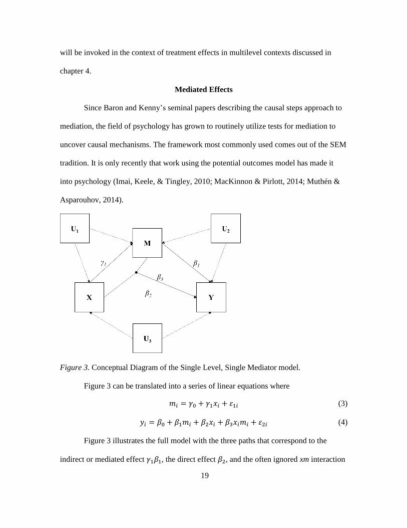
Figure 3. Conceptual Diagram of the Single Level, Single Mediator model.
Figure 3 can be translated into a series of linear equations where
𝑚𝑖 = 𝛾0 + 𝛾1𝑥𝑖 + 휀1𝑖 (3)
𝑦𝑖 = 𝛽0 + 𝛽1𝑚𝑖 + 𝛽2𝑥𝑖 + 𝛽3𝑥𝑖𝑚𝑖 + 휀2𝑖 (4)
Figure 3 illustrates the full model with the three paths that correspond to the
indirect or mediated effect 𝛾1𝛽1, the direct effect 𝛽2, and the often ignored xm interaction
20
term 𝛽3. Assume temporarily that the xm interaction term 𝛽3 is zero. In that case, the total
effect is the sum of the indirect effect 𝛾1𝛽1 and the direct effect 𝛽2. Figure 3 also includes
dashed lines from U1, U2, and U3 to signify the potential influence of unmeasured
confounders. The presence of these unmeasured confounders will be considered in the
discussion of assumptions necessary for the counterfactually defined effects.
Causal Definitions for Mediated Effects
The total effect is a central link between the traditional SEM approach to defining
causal effects and the counterfactual definition of causal effects. When the variables are
linearly related and there is no xm interaction (i.e., 𝛽3 is zero), then the traditional SEM
approach and the counterfactual approach produce the exact same estimates. However,
when there is a non-linear component, the traditional and counterfactual approaches
diverge (e.g. when there is an xm interaction, a binary or count mediator, or a binary or
count outcome; Muthén & Asparouhov, 2014).
Since the potential outcome for the individual in the case of two variables, X and
Y, is denoted as 𝑌𝑖(𝑥), the potential outcome in the case of three variables in the simplest
mediation model is 𝑌𝑖(𝑥, 𝑚).
𝐸[𝛿] = 𝑇𝑜𝑡𝑎𝑙 𝐸𝑓𝑓𝑒𝑐𝑡 = 𝐸[𝑌(1) − 𝑌(0)] (5)
𝐸[𝛿] = 𝑇𝑜𝑡𝑎𝑙 𝐸𝑓𝑓𝑒𝑐𝑡 = 𝐸[𝑌(1, 𝑀(1)) − 𝑌(0, 𝑀(0))] (6)
Equation 5 defines the average causal effect of X on Y from equation 2 as the
total effect of X on Y, while equation 6 partitions the total effect into the direct effect of
X and the indirect effect of X via M. Because the potential outcomes model defines the
decomposition using the expectation operator it is more general than the same
21
decomposition in the traditional SEM approach, which is defined using the covariance
and thus assumes a linear relation between the variables.
The potential outcome model also specifies two different ways to partition the
Total Effect (TE) depending on which direct or indirect effect is considered to be total
versus pure. While the naming is confusing, the distinction between total versus pure
effect rests on whether the xm interaction effect (𝛽3𝛾1) is considered. Pure effects do not
include the xm interaction term, while the corresponding total direct or indirect effect
does. The first decomposition for the Total Effect is the most common one used in the
literature, and defines the TE as the sum of the Pure Natural Direct Effect (PNDE) and
the Total Natural Indirect Effect (TNIE).
The PNDE is defined as:
𝑃𝑁𝐷𝐸 = 𝐸[𝑌(1, 𝑀(0)) − 𝑌(0, 𝑀(0))] (7)
Abstractly, the PNDE is defined as the difference between treatment and control
in Y when the value for the mediator is equal to the value obtained in the control
condition. In more concrete terms, the PNDE is the effect of the treatment if either 1) the
treatment’s effect on the mediator was blocked, or 2) the mediator was kept at the same
value as if there were no treatment at all (VanderWeele & Vansteelandt, 2009).
For the model specified in Figure 3, the PNDE translates into the following
quantities from equations 3 and 4:
𝑃𝑁𝐷𝐸 = 𝛽2 + 𝛽3𝛾0
It is easier to see with the model terms used that the direct effect is pure because it
does not include the xm interaction effect (𝛽3𝛾1). It is also easier to see that if the
interaction term is omitted, then the PNDE is the same as the traditional direct effect and

22
carries the same interpretation—namely, the effect of X on Y, holding the mediator
constant. If the xm interaction term is not omitted, the PNDE could be significant even if
𝛽2 = 0, because of the 𝛽3𝛾0 term.
The TNIE is defined as:
𝑇𝑁𝐼𝐸 = 𝐸[𝑌(1, 𝑀(1)) − 𝑌(1, 𝑀(0))] (8)
Abstractly the TNIE is defined as the difference in potential outcomes for
individuals in the treatment condition when the mediator is allowed to vary.
Using the same model specified in Figure 3, TNIE translates into the following
quantities from equations 3 and 4:
𝑇𝑁𝐼𝐸 = 𝛾1𝛽1 + 𝛽3𝛾1
As before with the PNDE, when the xm interaction term is omitted the TNIE is
equivalent to the indirect effect traditionally used in mediation analyses (𝛾1𝛽1). Also, just
like the PNDE, there can be an indirect effect even when 𝛽1 = 0, because of the included
interaction term.
The other possible decomposition of the TE is into the Total Natural Direct Effect
(TNDE) and the Pure Natural Indirect Effect (PNIE). The TNDE is defined as:
𝑇𝑁𝐷𝐸 = 𝐸[𝑌(1, 𝑀(1)) − 𝑌(0, 𝑀(1))] (9)
Abstractly, it can be thought of as being the direct effect when M is held constant
at the treatment condition instead of the control condition as compared with the PNDE.
Referring again to Figure 3 and equations 3 and 4:
𝑇𝑁𝐷𝐸 = 𝛽2 + 𝛽3𝛾0 + 𝛽3𝛾1
The effect is no longer pure because it includes the xm interaction effect (𝛽3𝛾1),
whereas the indirect effect is now considered pure.

23
The PNIE is defined as:
𝑃𝑁𝐼𝐸 = 𝐸[𝑌(0, 𝑀(1)) − 𝑌(0, 𝑀(0))] (10)
Abstractly the PNIE is measuring the difference in the potential outcomes for
individuals in the control group when the mediator is allowed to vary.
Lastly, referring again to Figure 3 and equations 3 and 4:
𝑃𝑁𝐼𝐸 = 𝛾1𝛽1
Here it is made clearer by the terms that this indirect effect is pure, because it only
considers the effect of X on Y via M.
The practical difference between the Total versus Pure Natural Indirect Effect is
that the TNIE tests whether the mediated effect is significant in the treatment group,
whereas the PNIE tests whether the mediated effect is significant in the control group.
The same is true for the Total versus Pure Natural Direct Effects, where the TNDE tests
whether the direct effect is significant for the treatment condition, whereas the PNDE
tests whether the direct effect is significant for the control condition.
Assumptions of the Counterfactually Defined Mediated Effects
There are four core assumptions underlying the previously defined effects (Valeri
& Vanderweele, 2013). First, there is no unmeasured confounding of the treatment-
outcome path, 𝛽2, as suggested by the presence of the unmeasured confounder U3 in
Figure 3. Second, there is no unmeasured confounding of the treatment-mediator path, 𝛾1,
as indicated by the paths emanating from the unmeasured confounder U1 in Figure 3.
When random assignment to treatment is used, the effects of U3 and U1 are assumed to be
ruled out.

24
Random assignment does not alleviate the burden of the next two assumptions,
which is why U2 is included in Figure 3. Third, there is no unmeasured confounding of
the mediator-outcome path, 𝛽2, as indicated by the paths from U2 in Figure 3. Fourth,
there is no effect of treatment on a mediator-outcome confounder (i.e., there is no path
from the treatment X to U2). Random assignment does nothing to resolve the third
assumption, which is often referred to as the sequential ignorability II assumption,
because individuals are not randomly assigned to levels of the mediator (MacKinnon &
Pirlott, 2014). Random assignment does nothing to resolve the fourth assumption,
because U2 is in essence an unmeasured potential mediator of the causal effect that has
been wrongly omitted. It is possible to probe the plausibility of the third assumption
using sensitivity analysis (Imai, Keele, & Yamamoto, 2010; MacKinnon & Pirlott, 2014).
It is also possible to address these two assumptions by developing more comprehensive
mediation models that include all of the potential mediators along with all of the potential
confounders.
Real Data Example
As noted in Chapter 1, some participants in the data set I am using here were
randomly assigned to not take part in any deliberations. This enables us to apply both the
traditional SEM direct and indirect effect tests along with the counterfactually defined
direct and indirect effects outlined above, absent the complications of a multilevel model.
The general research question posed in Chapter 1 asks whether the effect of
evidence strength on the juror’s Verdict-Confidence composite is mediated by the juror’s
perceptions of the plaintiff. In particular, the juror’s perceptions of Boyd’s selfishness.

25
With the jurors who were assigned to the non-deliberator condition, it is possible to test
this question using the single mediator, single level model.
Traditional SEM Defined Mediated Effects
Figure 4. Path Diagram for Single Mediator, Single Level Model.
Figure 4 replaces the X, M, and Y placeholders with the actual variables used.
SOE is the strength of evidence manipulation, with 0 coded as weak evidence and 1
coded as moderate evidence. The mediator is the juror’s self-reported perception of the
plaintiff Boyd’s selfishness. This is coded from 1 to 7, with 1 for “selfish” and 7 for
“concerned for others.” Finally, the dependent variable is a Verdict-Confidence
composite with -7 being completely confident in verdict for the Defense and 7 being
completely confident in verdict for the Plaintiff.
The mediation model was estimated using maximum likelihood with 5000
bootstrapped replications in Mplus 7.3, syntax provided in appendix B (Muthén &
Muthén, 2015). Three approaches were taken to estimate the causal effects. First, for
comparison, is the traditional method which assumes that there is no xm interaction.
Second, the counterfactual estimates excluding the interaction term are presented to
demonstrate the equivalency between the counterfactual and the traditional approaches.

26
Third, the counterfactual approach including the XM interaction term is presented. This
final model should produce different estimates of the causal effects. Table 3 and Figure 5
report the estimated causal effects using the traditional and counterfactual methods, along
with the bootstrapped 95% confidence intervals for the two approaches.
Table 3
Comparison of Traditional versus Counterfactually Defined Effects
Traditional Counterfactual,
No XM
Counterfactual,
With XM
Term Est. 95% CI Est. 95% CI Est. 95% CI
𝛾1 0.529 [0.203, 0.867] 0.529 [0.203, 0.867] 0.529 [0.203, 0.867]
𝛽1 0.836 [0.373, 1.295] 0.836 [0.373, 1.295] 0.585 [-0.117, 1.308]
𝛽2 1.481 [0.141, 2.827] 1.481 [0.141, 2.827] 1.499 [0.140, 2.835]
𝛽3 - - - - 0.456 [-0.458, 1.400]
Total Effect 1.924 [0.566, 3.224] 1.924 [0.566, 3.224] 1.924 [0.563, 3.224]
𝛾1𝛽1 0.442 [0.144, 0.927] - - - -
PNDE . - 1.481 [0.141, 2.827] 1.373 [0.233, 2.975]
TNIE - - 0.442 [0.144, 0.927] 0.551 [0.161, 1.209]
TNDE - - 1.481 [0.141, 2.827] 1.614 [0.233, 2.975]
PNIE - - 0.442 [0.144, 0.927] 0.310 [-0.011, 0.853]
Figure 5. Coefficient plot of the estimated causal effects from table 3.

27
Summary
The strength of evidence manipulation has a total effect of 1.924 on the Verdict-
Confidence DV when holding the mediator constant at the average score of 4.6. This
means that in the weak evidence condition the average Verdict-Confidence score was
-.613 or slightly in favor of the defense, while in the moderate evidence condition, the
average score was 1.311 or slightly in favor of the plaintiff.
The results of the mediation analysis are consistent for both the traditional and
counterfactually defined effects because the xm interaction term is not significant. The
results using the traditional approach suggest that the effect of evidence strength on
Verdict-Confidence is significantly mediated by the juror’s perceptions of Boyd’s
selfishness, with a significant indirect effect of .442. Thus, going from weak to moderate
evidence strength produced more positive assessments of Boyd, which in turn produced
greater confidence in and verdicts for the plaintiff, Boyd. This pathway implies that part
of evidence strength’s effect is due to its influence on how jurors evaluate the character
of the plaintiff.

28
CHAPTER 3
MULTILEVEL MODELS
There is a diversity of names used to describe multilevel models, such as
hierarchical linear models, random coefficient models, mixed effects models, or split-plot
designs. Multilevel models are used in a variety of disciplines to analyze data that have a
clustered or hierarchical structure, where one unit of analysis is nested or clustered with
another potential unit of analysis (Raudenbush & Bryk, 2001). In the case of jury
research, individual jurors are nested within a jury. Within this two-level structure,
convention would distinguish between the level-1 juror units and the level-2 jury units.
As with applying any statistical model, there are considerations for how to assess
the quality and utility of the model as well as important assumptions that underlie their
use. A full discussion of these factors is a dissertation in its own right and would distract
from the discussion of the pieces of multilevel models that are essential to the causal
inference (Raudenbush & Bryk, 2001). As such, this chapter will focus on discussing the
sources of variation in multilevel models, estimation and interpretation of contextual
effects, and the role of centering.
Sources of Variation, Contextual Effects, and Centering
In combined model notation, the multilevel model with a single level-1 predictor
can be written as follows:
𝑦𝑖𝑗 = 𝛽0 + 𝛽1𝑥𝑖𝑗 + 𝑢𝑜𝑗 + 휀𝑖𝑗 (11)
Where yij and xij are the level-1 outcome and predictor, β0 and β1 are the intercept
and slope coefficients, u0j is the level-2 residual deviations that allow the intercepts (β0)
to vary across clusters, and εij is the within-cluster error term.
29
It is important to note that yij and xij have two sources of variability that can be
decomposed in the following manner.
𝑦𝑖𝑗 − �̅� = (𝑦𝑖𝑗 − �̅�𝑗) + (�̅�𝑗 − �̅� ) (12)
𝑥𝑖𝑗 − �̅� = (𝑥𝑖𝑗 − �̅�𝑗) + (�̅�𝑗 − �̅� ) (13)
That is to say, deviations of the individual’s score from the grand mean can be
partitioned into deviations of the individual’s score from the cluster mean and deviations
of the cluster mean from the grand mean. This should look intuitively familiar from
ANOVA, as the total deviation decomposes into within-cluster and between-cluster
variation.
Because the multilevel framework enables the modeling of both within and
between clusters relations, there are two possible sources of association for yij and xij:
within-cluster, between-cluster, or both. Critically, equation 11 assumes that the level-1
and level-2 regressions are identical because it uses a single slope coefficient, β1.
Violating this assumption means that β1 will be a weighted average of two associations
and might not be indicative of either. Specifically, the weighting is determined by the
magnitude of the predictor’s ICC, such that only when the predictor’s ICC equals zero is
β1 in equation 11 the correct estimate of the average within-cluster regression of y on x
(Raudenbush & Bryk, 2001, pp. 135-139). See also appendix C for a more detailed
discussion of ICC, design effects, and effective sample sizes.

30
To properly disentangle the within- and between-cluster associations of yij and xij
an additional variable and regression slope needs to be added to equation 11.
𝑦𝑖𝑗 = 𝛽0 + 𝛽1𝑥𝑖𝑗 + 𝛽2𝑥𝑗 + 𝑢𝑜𝑗 + 휀𝑖𝑗 (14)
Here β2 refers to the regression slope for the cluster means xj. When added in this
form β1 is a partial regression coefficient that represents the unique level-1 influence of x,
controlling for the level-2 cluster means. β2 is a partial regression coefficient that
represents the difference between the level-2 regression coefficient and the level-1
regression coefficient. In this form, β2 is the contextual effect estimate.
It is important to note that these interpretations of the regression coefficients do
not change if the level-1 predictor is uncentered or centered at the grand mean of x.
However, if the predictor is instead centered at the cluster mean, then β1 and β2 take on
slightly different meanings. Centering within cluster effectively partitions the within-
cluster and between-cluster variability. As such, β1 is the estimate of the pooled within-
cluster slope, while β2 is now just the between-cluster regression slope of the outcome
means on the predictor means, and no longer represents the difference between level-2
and level-1 regression coefficients (Feaster, Brincks, Robbins, & Szapocznik, 2011).
However, in this case, β1 can be subtracted from β2 to produce the same estimate
of the contextual effect as before. This equivalency exists because of the following
mathematical relation among the regression coefficients.
𝛽𝐶𝑜𝑛𝑡𝑒𝑥𝑡𝑢𝑎𝑙 𝐸𝑓𝑓𝑒𝑐𝑡 = 𝛽𝐵𝑒𝑡𝑤𝑒𝑒𝑛 𝐶𝑙𝑢𝑠𝑡𝑒𝑟 − 𝛽𝑊𝑖𝑡ℎ𝑖𝑛 𝐶𝑙𝑢𝑠𝑡𝑒𝑟 (15)
Real Data Example
As described in Chapter 1, the Searle dataset has juror-level measures of the
perceived selfishness mediator and the outcome composite of Verdict-Confidence. Using

31
Mplus 7.3 to estimate the multilevel model, the ICC for the mediator was .084 and the
ICC for the DV was .045. These values indicate that approximately 8% of the variability
in the mediator and 5% of the variability in the DV is attributable to variability between
the juries. As noted above, by centering individual scores within each cluster it is possible
to decompose the correlation of the mediator with the DV into the within-cluster and
between-cluster components (see Figure 6).
Figure 6. Within-Cluster versus Between-Cluster Sources of Variability.
The Within panel shows the regression slope for the individual Verdict-
Confidence composite on individual perceived greediness of the plaintiff. In the Between
panel are the aggregated means of both the mediator and DV and the jury-level regression
slope, which appears to be stronger than the within-level. If the jury-level regression

32
slope is significantly different from the juror-level regression slope, that difference would
be interpreted as evidence for a contextual effect.
In the case of the mediator and the DV there does appear to be a significant
contextual effect. The estimated within or juror-level regression of Verdict-Confidence
on perceived selfishness is .465 (.193), p = .016. Thus, for an individual juror, the more
the juror perceived Boyd as being less selfish and more concerned about others, the
stronger the juror's confidence in returning a verdict for Boyd. At the jury-level, the
regression of the jury’s average Verdict-Confidence on the jury’s average perceived
selfishness is 1.712 (.336), p < .001. Thus, at the jury-level, as the jury perceived the
plaintiff Boyd as being less selfish and more concerned about others the jury increased its
confidence in returning a verdict for Boyd.
The contextual effect as calculated by the difference between these regression
coefficients of 1.712 and .465 is significant and equal to 1.247 (.395), p = .002. This
would be interpreted as 1) the jury-level effect of perceived selfishness on Verdict-
Confidence is significantly stronger than the juror-level effect; 2) there is a significant
effect of the jury on the relationship between the juror’s perception of the plaintiff’s
selfishness and the juror’s Verdict-Confidence score.

33
Figure 7. The Effect of Grand versus Group Mean Centering.
Figure 7 highlights the role of centering. When grand mean centering is used, the
juror-level perceived selfishness scores are still strongly correlated with the jury-level
Verdict-Confidence composite. In contrast, the second panel shows that once each
individual score is centered at the group mean, the cross-level effect is gone.
Traditional SEM Defined Mediated Effects
Work on multilevel mediation models has existed for some time using the
traditional SEM approaches outlined in Chapter 2. This approach will be discussed
further in Chapter 4. For now it is sufficient to define the essential equations for
estimating a jury-only mediation model, or as is commonly referred to in the literature, a
2-2-2 mediation model.
𝑚𝑖𝑗 = 𝛾0 + 𝛾1𝑥𝑗 + 𝑢0𝑗 + 휀𝑖𝑗 (16)
𝑦𝑖𝑗 = 𝛽0 + 𝛽1𝑚𝑖𝑗 + 𝛽2𝑚𝑗 + 𝛽3𝑥𝑗 + 𝑢1𝑗 + 휀𝑖𝑗 (17)

34
As before, the traditional SEM approach defines the mediated effect as the
product-of-coefficients, or in this case, as coefficients γ1β2. In Figure 8, to facilitate
drawing connections across the different approaches used, I’ve elected to mark the paths
separately from the coefficients (i.e., path a2 is equal to γ1 in equation 16). This is done
because in future models, the paths will not perfectly coincide with the coefficients used
to estimate them, unlike in the single level analysis.
Figure 8. Conceptual Model of Traditional 2-2-2 analysis.
To make salient the role of clustering and contextual effects, the mediation model
was analyzed two ways. When analyzed correctly, the mediator was centered at the group
mean to ensure that the b2 path was the between-jury effect and not the contextual effect.
When analyzed incorrectly, the clustering was ignored which resulted in only a single b
path being estimated.

35
The correctly analyzed mediated effect is .633 (0.229), p = .006. This means that
juries assigned to the moderate evidence strength condition had a .633 increase in the
jury’s mean Verdict-Confidence score as mediated by the jury’s rating of Boyd’s
selfishness, as summarized in Table 4 and Figure 9.
Table 4
Traditional 2-2-2 Models Analyzed With vs Without Respect to Clustering
Correctly Analyzed Incorrectly Analyzed
est s.e. 95% CI est s.e. 95% CI
a2 0.416 0.116 [0.188, 0.644] 0.407 0.103 [0.214, 0.614]
b1 0.463 0.194 [0.083, 0.842] 0.701 0.169 [0.382, 1.035]
b2 1.520 0.337 [0.861, 2.180]
c’ 0.675 0.418 [-0.144, 1.494] 1.019 0.441 [0.121, 1.897]
a2b2 0.633 0.229 [0.184, 1.083] 0.285 0.093 [0.135, 0.510]
Figure 9. Coefficient plot of estimated MLM mediated effects in Table 4.

36
Comparative Analysis Ignoring Clustering
When analyzed incorrectly, the mediated effect is .285 (0.093), p = .002.
However, this mediated effect has no clear meaning for several reasons.
First, the a2 paths are not equivalent across the two analyses because in the correct
analysis the DV is the cluster means, while when incorrectly analyzed the DV is the
individual juror scores. This produces not only a different estimated quantity, but also has
the effect of decreasing the standard error to .103 when done incorrectly versus the
correct standard error of .116. This occurs because the sample size of the a2 path for the
correct analysis is all 120 juries, whereas the sample size of the a2 path in the incorrect
analysis is all 705 jurors. Thus, ignoring clustering has a two-fold effect such that the
estimate is of a different quantity, and the standard error of the incorrect analysis is also
smaller. While the standard error is only slightly smaller in this case, ignoring clustering
can produce meaningful alpha inflation.
Second, when clustering is ignored the b path in the incorrect analysis is now a
weighted average of the between b2 and within b1 regression coefficients. In this case, the
b path is noticeably smaller than b2 and as such the mediated effect is noticeably smaller.
The b path also suffers from the same underestimation of the standard errors. However,
most importantly, by ignoring the clustering the b path is now confounded by the group
differences. That is, by ignoring clustering an “unmeasured” confounder of the mediator
to DV link has been introduced.
Lastly, because the incorrect analysis underestimates the mediated effect the
direct effect (c’) is incorrectly estimated as being 1.019 rather than 0.675. Moreover, the
significance versus non-significance of the direct effect raises interpretative questions.

37
Summary
At the jury-level, the strength of evidence manipulation has a total effect of 1.308
on the jury’s average Verdict-Confidence rating, when holding the mediator constant at
the jury-level grand mean of 4.581. This means that in the weak evidence condition,
juries on average reported a Verdict-Confidence score of -.424, or slightly in favor of the
defense, while juries in the moderate evidence condition reported an average score of
.885, or slightly in favor of the plaintiff.
The results of the jury-level mediation analysis are consistent with the non-
deliberating juror analysis from Chapter 2. The significant a2b2 effect of .633 suggests
that a jury’s aggregate perception of Boyd’s selfishness mediated the effect of evidence
strength on the jury’s aggregate Verdict-Confidence rating. Thus, at the jury-level, going
from weak to moderate evidence strength produced more positive aggregate assessments
of Boyd, which in turn produced greater confidence in and verdicts for the plaintiff,
Boyd.
38
CHAPTER 4
INTEGRATED MLM MEDIATION MODELS
Although work on multilevel mediation models has existed for some time (Krull
& MacKinnon, 1999; Krull & MacKinnon, 2001), there has been some disagreement in
the methodological literature about how to think about cross-level mediation (Preacher et
al., 2010). One camp advocates that cross-level mediation where effects are transmitted
between levels is not possible (Preacher et al., 2010). For example, take the Searle dataset
wherein juries are randomly assigned to either weak versus moderate evidence. Preacher
and colleagues would argue that, because everyone within a jury received the same
treatment, there can be no meaningful within-jury variability and so no transmission from
level-2 to level-1. The opposing camp argues that the interpretation of the contextual
effect as the effect of the cluster upon the individual does imply that there can be cross-
level mediation (Krull & MacKinnon, 1999; Krull & MacKinnon, 2001; Pituch &
Stapleton, 2012), and work using the potential outcomes model shows that such an
inference is justified under certain assumptions (VanderWeele, 2010).
Revisiting Contextual Effects
Contextual effects are interpreted as the change in the outcome variable
attributable to the different contexts in which the level-1 unit is placed (Feaster et al.,
2011; Raudenbush & Bryk, 2001). So far, contextual effects have been defined using
predictors that operate on both level-1 and level-2. However, work done by VanderWeele
(2010) shows that it is possible to define a contextual effect with a randomized level-2
intervention using the potential outcomes framework.

39
Take equation 11 and replace xij with a cluster randomized experimental
manipulation Tj where 0 represents the control condition and 1 represents the treatment
condition.
𝑦𝑖𝑗 = 𝛽0 + 𝛽1𝑇𝑗 + 𝑢𝑜𝑗 + 휀𝑖𝑗 (18)
β1 has the standard dummy coded interpretation as the difference in the mean
scores of the treatment versus control condition. The standard interpretation of β1 is as a
between-cluster effect; however, β1 of equation 11 is also the causal effect estimate of the
cluster level treatment on individuals, if the following assumptions hold (VanderWeele,
2010; VanderWeele, 2008). First is the obvious but necessary consistency assumption
that states that the potential outcome for an individual in a given treatment condition is
equal to the observed outcome for the individual in the given treatment condition. Second
is the neighborhood-level stable unit treatment value assumption, which states that only
the treatment assignment of the participant’s cluster and no other cluster’s treatment
assignment influences the individual’s outcome. This could be violated if treatment
clusters begin implementing parts of interventions from other treatment conditions, like
combining different drug therapies. The third assumption is that the cluster remains
intact, that is, the cluster intervention does not change the cluster membership. For
example, if differential attrition occurs in treatment versus control due to the treatment.
To see why this is also interpretable as a contextual effect, we substitute βwithin
cluster = 0 into equation 15 because everyone in a cluster receives the same treatment
condition and so treatment does not vary within clusters (Pituch & Stapleton, 2012). This
means that the contextual effect is now equal to the between-cluster effect and this

40
equivalence means that β1 from equation 18 can be interpreted as either an effect on
clusters (βbetween cluster) or a cross-level effect on individuals (βcontextual effect).
The Role of Centering in Defining Cross-Level Mediated Effects
Pituich and Stapelton (2012) argue that the presence of cross-level mediated
effects depends on the theoretical nature of the constructs. First, it must be possible for
the jury-level effect to influence the individual-level mediator. That is, there must be
some theoretical reason to believe that the strength of the evidence presented in a trial can
influence the individual juror’s psychological processes. In contrast, manipulating
something like the jury size does not seem to implicate an individual juror’s
psychological processes.
Second, the mediating variable must represent absolute scale levels and not
relative standing within a cluster. This is the role that deciding between grand mean
versus group mean clustering plays. When using raw or grand mean centered scores, the
implication is that the underlying psychological process occurs on an absolute scale and
that there is no reference to the other group member scale scores. For example, say a jury
intervention like note taking is designed to increase juror comprehension of the scientific
evidence presented at trial by decreasing the number of recall errors made. The mediation
process here occurs through the individual mediator when one assumes that improved
juror comprehension is brought about by lower absolute number of recall errors.
In comparison, group mean centering implies that what matters is the relative
position of the individual within the group. When the hypothesized mechanism involves
the relative position of jurors within juries, then the use of cross-level mediation is
inappropriate. For example, take a different mediator where jurors are asked to provide

41
ratings of their relative understanding of the evidence. In this example, increases in juror
comprehension are thought to be greater because the individual jurors perceive
themselves as understanding the evidence presented relative to the other jurors, not
because of the absolute scale value.
Thus, if the mediator is theorized as involving the relative standing within a
cluster, then computing any indirect effect via the level-1 b1 path is not possible. This is
because in equation 19, the treatment averages of what would be the a1 path would all
equal zero, as would the a1 path. This is where Pituich and Stapelton (2012) agree with
Preacher’s assessment that the treatment effect “cannot account for individual differences
within a group,” as the group mean deviation scores represent (Preacher, YEAR, p. xx).
Treatment effects of this kind of design can only be mediated by group means, as
illustrated in Figure 8.
𝑚𝑖𝑗 = 𝛾0 + 𝛾1𝑥𝑗 + 𝑢0𝑗 + 휀𝑖𝑗 (19)
𝑦𝑖𝑗 = 𝛽0 + 𝛽1𝑚𝑖𝑗 + 𝛽𝑐𝑚𝑗 + 𝛽3𝑥𝑗 + 𝑢1𝑗 + 휀𝑖𝑗 (20)
Cross-Level Mediators
As discussed in Chapter 1, the potential outcomes model gives rise to two new
mediated effects stemming from the counterfactual interpretation of the contextual effect
of the level-2 treatment variable and the contextual effect of the mediator. The a1b1
indirect effect is a context-free indirect effect in the sense that when the βc coefficient is
present in equation 20, then the β1 coefficient in equation 19 is free from the effect of
jury-level differences. In comparison, the a2bc indirect effect is the contextualized effect
of the group on the individual-level outcome variable. That is, the level-2 treatment effect
42
changes the context in which the individual is embedded within, which also influences
the individual outcome variable.
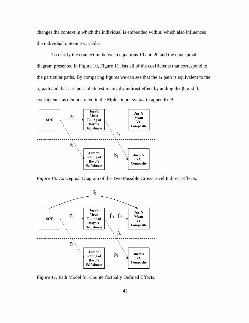
To clarify the connection between equations 19 and 20 and the conceptual
diagram presented in Figure 10, Figure 11 lists all of the coefficients that correspond to
the particular paths. By comparing figures we can see that the a1 path is equivalent to the
a2 path and that it is possible to estimate a2b2 indirect effect by adding the β1 and βc
coefficients, as demonstrated in the Mplus input syntax in appendix B.
Figure 10. Conceptual Diagram of the Two Possible Cross-Level Indirect Effects.
Figure 11. Path Model for Counterfactually Defined Effects.

43
CHAPTER 5
DATA ANALYSIS AND RESULTS
This chapter will discuss the results for the a1b1, a2bc, and a2b2 indirect effects, as
summarized in Table 5 and Figure 12. It will also provide a test and discussion for the
difference between the a1b1 indirect effect for the non-deliberators versus the
counterfactually defined cross-level a1b1 indirect effect.
Table 5
Comparison of Mediated Effects
Non-Deliberators
1-1-1 model
Jury Only
2-2-2
Counterfactually
Defined Indirect Effects
est s.e. 95% CI est s.e. 95% CI est s.e. 95% CI
a1 0.529 .171 [0.203, 0.867] - - - 0.416 .116 [0.188, 0.644]
a2 - - - 0.416 .116 [0.188, 0.644] 0.416 .116 [0.188, 0.644]
b1 0.836 .235 [0.373, 1.295] 0.463 .194 [0.083, 0.842] 0.478 .191 [0.104, 0.851]
b2 - - - 1.520 .337 [0.861, 2.180] 1.525 .337 [0.866, 2.184]
bc - - - - - - 1.047 .394 [0.274, 1.820]
c’ 1.481 .657 [0.141, 2.827] 0.675 .418 [-0.144, 1.494] 0.677 .418 [-0.142, 1.496]
a2b2 - - - 0.633 .229 [0.184, 1.083] 0.635 .230 [0.185, 1.085]
a1b1 0.442 .193 [0.144, 0.927] - - - 0.199 .093 [0.016, 0.382]
a2bc - - - - - - 0.436 .211 [0.023, 0.849]
Figure 12. Coefficient plot summarizing the various mediated effects in Table 5.

44
Overview of Mediated Effects
Counterfactually Defined Indirect Effects
As a brief overview, the total effect of evidence strength on Verdict-Confidence is
mediated by perceptions of Boyd’s selfishness in three different ways.
First, focusing solely at the jury-level, those juries in the moderate evidence
condition saw a .635 increase in the jury’s aggregate Verdict-Confidence rating as a
function of the jury’s aggregate perception of Boyd’s selfishness.
Second, changes in the jury’s perception of Boyd’s selfishness caused by the
evidence strength manipulation resulted in a .436 increase in the individual juror’s
Verdict-Confidence.
Third, the evidence strength manipulation produced a .199 increase in the
individual juror’s Verdict-Confidence rating by changing the individual juror’s
perception of Boyd’s selfishness.
Ecological Validity Tests
Because both deliberators and non-deliberators were measured on the same
variables and randomly assigned to deliberation status, it is possible to test the difference
in the indirect effects using a simple z-test with the standard error of the difference given
in equation 5.9 of MacKinnon’s 2008 book:
𝑆�̂�1�̂�1−�̂�2�̂�2= √𝑆2
�̂�1�̂�1+ 𝑆2
�̂�2�̂�2− 2�̂�1�̂�2𝑆�̂�1�̂�2
2
where 𝑆2�̂�1�̂�1
refers to the squared standard error for the first indirect effect,
𝑆2�̂�2�̂�2
refers to the squared standard error for the second indirect effect, and 2�̂�1�̂�2𝑆�̂�1�̂�2
is a term designed to adjust for the covariance of the estimates of the b1 and b2

45
coefficients, but it is not applicable in this case because of the separate estimation of the
two indirect effects. As such, the standard error reduces to
𝑆�̂�1�̂�1−�̂�2�̂�2= √𝑆2
�̂�1�̂�1+ 𝑆2
�̂�2�̂�2
2
The difference between the indirect effects for the deliberators and non-
deliberators is .243 and the standard error for the difference is .214, which results in a z-
test value of 1.134, p = .209. This suggests that there was no significant effect of
deliberation status on the mediated effects and that there might not be a general threat to
ecological validity by using non-deliberating jurors in this instance.
Summary and Synthesis of Mediated Effects
All three indirect effects were significant, but as discussed in previous chapters,
each has a different meaning. The a1b1 indirect effect of .199, 95%CI[.016, .382], means
that going from weak to moderate evidence strength produced a .2 of a point increase in
the juror’s Verdict-Confidence rating as mediated by the juror’s ratings of the plaintiff’s
selfishness. Importantly, this mediated effect is free of the jury’s influence, which has
been partialed out by the contextual effect and is accounted for in the a2bc indirect effect.
Thus the a1b1 effect is the estimate of the mediated effect for the individual juror assigned
to deliberate in a jury, which is why it serves as the comparison to the non-deliberators
for the ecological validity test.
In comparison, the a2bc indirect effect of .436, 95%CI[.023, .849], means that
going from weak to moderate evidence strength produced about a .4 of a point increase in
the juror’s Verdict-Confidence rating as mediated by the jury’s mean ratings of the
plaintiff’s selfishness. That is, the strength of evidence manipulation produced a change

46
in the jury-level mediator, which exerts a contextual effect on the individual juror. Thus,
the a2bc indirect effect is the effect the jury-level changes in the mediator exert on the
individual juror.
Next, the a2b2 indirect effect of .635, 95%CI[.185, 1.085], means that going from
weak to moderate evidence strength produced about a .6 of a point increase in the jury’s
average Verdict-Confidence rating as mediated by the jury’s mean ratings of the
plaintiff’s selfishness.
Finally, the comparison of the mediated effect for deliberators (.199) versus non-
deliberators (.442) results in a non-significant difference, which suggests that the
mechanism functions similarly at the individual-level regardless of deliberation status.
However, the significant a2bc mediated effect suggests that being in a group does exert its
own unique influence. Taken together, the results suggest that it would be ecologically
valid to study the individual (a1b1) mechanism outside of mock juries with the
understanding that there is also a unique contextual effect of being in a jury on the
individual (a2bc).

47
CHAPTER 6
IMPLICATIONS AND EXTENSIONS
While this project has demonstrated the immediate benefits of adopting the
specific counterfactually defined cross-level mediated effects, adopting this framework
also provides a way forward for dealing with some of the complexities in mock jury
research. In this chapter, I summarize the implications of this framework and touch on a
few of those future applications.
Implications for the Design of Mock Jury Research
Adopting this framework opens up a variety of possible mediated effects to be
studied beyond the 2-1-1 and 2-2-1 models described here.
Timing of Measurements
The timing of measurement for the mediator and dependent variable, either
before, during, or after deliberation, has implications for the contextual effect and thus
the a2bc mediated effect. This also has implications for the kind of questions that can be
asked using a repeated measures design, which I also discuss below.
Mediator and DV measured before deliberation. When both variables are
measured before deliberation, then the contextual effect likely represents non-verbal cues,
such as head nods to certain arguments made or other information that is leaked by jury
members (e.g., gender or race).
Mediator measured before deliberation and DV measured after. When the
mediator and the DV are split in this fashion, then the contextual effect likely represents
how the starting position of a jury influences the course of the deliberation and the DV
after deliberation.

48
Mediator and DV measured after deliberation. When both are measured after
deliberation has occurred, the contextual effect likely represents how the ending position
of a jury directly influences the DV.
Use of Deliberation Manipulation
As described in the ecological validity sections, randomly assigning jurors to
either deliberate in a jury or not can provide useful information about the individual intra-
psychological mechanisms.
Measurement of Mediators and Outcomes
As noted in Chapter 4, the manner in which a variable is measured influences how
the variable functions as a mediator or outcome variable. Thinking carefully about how
and what the variable measures matters, and it is important to think in terms of juror- or
jury-level traits and in terms of a juror’s absolute versus relative standing.
Juror-level measures of a jury-level construct. If individual jurors are asked to
rate how cohesive or divisive the deliberation experience was, those individual level
ratings are not reflective of an individual-level construct. Thus, a jury-level trait can be
constructed from questions answered by individual jurors, but it should only serve as a
jury-level mediator or DV. For example, the jury’s verdict is a function of the votes of
individual jurors, but the jury’s verdict only exists at the jury-level.
Absolute versus relative standing. If, for example, the mediator is theorized to
depend upon the relative standing of a juror within a jury, it is not possible to estimate
either the a1b1 or a2bc cross-level mediated effects. This is because relative standing
requires group mean centering to be used, which, as illustrated in Figure 7, removes the
link between the juror- and jury-levels.

49
Non-normal Mediators and Dependent Variables
As discussed above, part of the purpose of moving to this framework for assessing
mediation is that it enables a whole variety of new cross-level mediated effects to be
estimated. Another benefit is that it enables a whole new set of variables to be used as
mediators and dependent variables.
Dealing with verdicts. Part of my critique of the Verdict-Confidence composite
in appendix A stems from it being an unnecessary complication when attempting to deal
with the binary nature of verdicts. While I have opted to utilize the Verdict-Confidence
composite in this project for illustrative purposes, the counterfactually defined mediated
effects in single-level models for binary outcomes already exist. The newest versions of
Mplus can already automatically compute these effects (Muthén & Asparouhov, 2014).
However, work still needs to be done in extending these effects to the multilevel context.
Dealing with damage awards. Effectively modeling damage awards is a difficult
task. Jurors are notorious for giving highly variable awards. Although a variety of
proposals have been made for how to deal with the variability in awards, I believe this
framework encourages adopting newer statistical procedures because the definition of the
mediated effects are not tied to their estimation as in the traditional SEM framework. For
example, we can adopt a method that is more robust to extreme values like quantile
regression, where the median replaces the mean. This has already been discussed as an
option in the psychology literature as a more robust alternative to the traditional methods
(Yuan & Mackinnon, 2014). When estimated in a fully Bayesian setting, some of the less
statistically favorable recommendations, like dropping or trimming the extreme values or
discarding missing values, can be ignored.

50
Alternatively, there exists a class of loglinear variance models (i.e., models of
conditional variance) that enable the variance to be modeled directly (Cook & Weisberg,
1983, 1999). Work in these models paralleled work on the generalized linear models that
unified linear, logistic, and Poisson regression under a common framework. Loglinear
variance models, however, are more flexible in the sense that they allow for predictors for
both the mean function and the variance function. These kinds of models enable jury
researchers to take what was a severe statistical problem and turn it into a new source of
research questions. For example, even if the average damage awards provided by juries
who are able to take notes do not statistically differ from juries who cannot take notes, it
could still be the case that juries who take notes have lower variability in damage awards
than juries who do not take notes. Moreover, the generality of the potential outcomes
model means that we should be able to use the same general definitions outlined in
Chapter 2 to estimate mediated effects for the conditional variances.
Longitudinal Mediation
If jury researchers are interested in exploring how the unfolding of deliberation
influences jury decision-making, there are longitudinal mediation models available. The
simplest model would be a pre-post deliberation design with two time points. By
capturing the mediator at both ends of the deliberative process, it is possible to test how
the starting and end points of the deliberation influence the juror-level dependent
variable. More complicated models with more measurement points could be treated as
being nested within individual jurors who are nested within juries (MacKinnon &
Valente, 2014).

51
Implications of the Verdict-Confidence DV
Although I provide a fuller critique of the Verdict-Confidence DV in appendix A,
I believe it is necessary to briefly discuss the implications of using it as my primary
outcome variable. While the substantive use and interpretations of the cross-level
mediated effects are unaffected, the specific standard errors and p-values for the mediated
effects are all likely too small. Appendix A discusses the reasons for that in some depth.
These issues of statistical conclusion validity are also likely magnified by the strong
assumption in multilevel models that the residuals are normally distributed.
Conclusion
The primary goals of this dissertation were to provide an encapsulated summary
of two very different statistical models that enables substantive jury researchers to use
these specific cross-level mediated effects and tests of ecological validity in earnest.
Along the way, serious statistical problems with the commonly used Verdict-Confidence
measure were uncovered and catalogued.
The a1b1 and the a2bc mediated effects are only two the many possible cross-level
mediated effects that might be of interest to substantive jury researchers. By being aware
of the methodological advances in causal inference, substantive jury researchers should
be able to engage quantitative psychologists. This engagement is necessary as the
ossification of quantiative knowledge within jury research makes for rigid and eventually
brittle substantive theory.

52
REFERENCES
Baron, R. M., & Kenny, D. A. (1986). The moderator-mediator variable distinction in
social psychological research: conceptual, strategic, and statistical considerations.
Journal of Personality and Social Psychology, 51(6), 1173–1182.
http://doi.org/10.1037/0022-3514.51.6.1173
Bornstein, B. H., & Greene, E. (2011). Jury Decision Making: Implications For and From
Psychology. Current Directions in Psychological Science, 20(1), 63–67.
http://doi.org/10.1177/0963721410397282
Cook, R. D., & Weisberg, S. (1983). Diagnostics for heteroscedasticity in regression.
Biometrika, 70(1), 1–10. http://doi.org/10.1093/biomet/70.1.1
Cook, R. D., & Weisberg, S. (1999). Applied Regression Including Computing and
Graphics. Wiley-Interscience.
Devine, D. J. (2012). Jury Decision Making: The State of the Science. NYU Press.
Devine, D. J., Buddenbaum, J., Houp, S., Studebaker, N., & Stolle, D. P. (2009). Strength
of evidence, extraevidentiary influence, and the liberation hypothesis: Data from the
field. Law and Human Behavior, 33(2), 136–148. http://doi.org/10.1007/s10979-
008-9144-x
Devine, D. J., Clayton, L. D., Dunford, B. B., Seying, R., & Pryce, J. (2001). Jury
decision making: 45 years of empirical research on deliberating groups. Psychology,
Public Policy, and Law, 7(3), 622–727. http://doi.org/10.1037/1076-8971.7.3.622
Diamond, S. S., Saks, M. J., & Landsman, S. (1998). Juror Judgments about Liability and
Damages: Sources of Variability and Ways to Increase Consistency. Depaul Law
Review, 48(2), 301–326.
Feaster, D., Brincks, A., Robbins, M., & Szapocznik, J. (2011). Multilevel models to
identify contextual effects on individual group member outcomes: A family
example. Family Process, 50(2), 167–183. http://doi.org/10.1111/j.1545-
5300.2011.01353.x
Imai, K., Keele, L., & Tingley, D. (2010). A general approach to causal mediation
analysis. Psychological Methods, 15(4), 309–334. http://doi.org/10.1037/a0020761
Imai, K., Keele, L., & Yamamoto, T. (2010). Identification, Inference and Sensitivity
Analysis for Causal Mediation Effects, 25(1), 51–71. http://doi.org/10.1214/10-
STS321

53
Imai, K., King, G., & Stuart, E. a. (2008). Misunderstandings between experimentalists
and observationalists about causal inference. Journal of the Royal Statistical Society.
Series A: Statistics in Society, 171(2), 481–502. http://doi.org/10.1111/j.1467-
985X.2007.00527.x
Imai, K., & van Dyk, D. a. (2004). Causal Inference With General Treatment Regimes.
Journal of the American Statistical Association, 99(467), 854–866.
http://doi.org/10.1198/016214504000001187
Judd, C. M., & Kenny, D. A. (1981). Process Analysis: Estimating Mediation in
Treatment Evaluations. Evaluation Review.
http://doi.org/10.1177/0193841X8100500502
Kalven, H., & Zeisel, H. (1971). The American Jury. University of Chicago Press.
Krull, J. L., & MacKinnon, D. P. (1999). Multilevel mediation modeling in group-based
intervention studies. Evaluation Review, 23(4), 418–444.
http://doi.org/10.1177/0193841X9902300404
Krull, J., & MacKinnon, D. (2001). Multilevel modeling of individual and group level
mediated effects. Multivariate Behavioral Research, 36(June 2015), 249–277.
http://doi.org/10.1207/S15327906MBR3602
Landsman, S., Diamond, S., Dimitropoulos, L., & Saks, M. J. (1998). Be Careful What
You Wish for: The Paradoxical Effects of Bifurcating Claims for Punitive Damages.
Wisconsin Law Review.
MacKinnon, D. P. (2008). Introduction to Statistical Mediation Analysis. Routledge
Academic.
Mackinnon, D. P., & Dwyer, J. H. (1993). Estimating Mediated Effects in Prevention
Studies. Evaluation Review. http://doi.org/10.1177/0193841X9301700202
MacKinnon, D. P., & Pirlott, A. G. (2014). Statistical Approaches for Enhancing Causal
Interpretation of the M to Y Relation in Mediation Analysis. Personality and Social
Psychology Review. http://doi.org/10.1177/1088868314542878
MacKinnon, D. P., & Valente, M. J. (2014). Mediation from Multilevel to Structural
Equation Modeling. Annals of Nutrition and Metabolism, 65(2-3), 198–204.
http://doi.org/10.1159/000362505
Morgan, S. L., & Winship, C. (2014). Counterfactuals and Causal Inference: Methods
and Principles for Social Research. Cambridge University Press.

54
Muthén, B. O., & Asparouhov, T. (2014). Causal Effects in Mediation Modeling: An
Introduction with Applications to Latent Variables. Structural Equation Modeling,
(June), 1–48. http://doi.org/10.1080/10705511.2014.935843
Muthén, L. K., & Muthén, B. O. (2015). Mplus. The comprehensive modelling program
for applied researchers: User’s guide, 7.3.
Pennington, N., & Hastie, R. (1993). Reasoning in explanation-based decision making.
Cognition, 49(1-2), 123–163. http://doi.org/10.1016/0010-0277(93)90038-W
Pennington, N., & Hastie, R. (1994). Inside the Juror: The Psychology of Juror Decision
Making. Cambridge University Press.
Pituch, K. a., & Stapleton, L. M. (2012). Distinguishing Between Cross- and Cluster-
Level Mediation Processes in the Cluster Randomized Trial. Sociological Methods
& Research, 41(4), 630–670. http://doi.org/10.1177/0049124112460380
Preacher, K. J., Zyphur, M. J., & Zhang, Z. (2010). A general multilevel SEM framework
for assessing multilevel mediation. Psychological Methods, 15(3), 209–233.
http://doi.org/10.1037/a0020141
Raudenbush, S. W., & Bryk, A. S. (2001). Hierarchical Linear Models: Applications and
Data Analysis Methods. SAGE Publications, Inc.
Ruva, C. L., & Guenther, C. C. (2015). From the shadows into the light: How pretrial
publicity and deliberation affect mock jurors’ decisions, impressions, and memory.
Law and Human Behavior, 39(3), 294–310. http://doi.org/10.1037/lhb0000117
Stasser, G. (1988). Computer simulation as a research tool: The DISCUSS model of
group decision making. Journal of Experimental Social Psychology, 24(5), 393–422.
http://doi.org/10.1016/0022-1031(88)90028-5
Valeri, L., & Vanderweele, T. J. (2013). Mediation analysis allowing for exposure-
mediator interactions and causal interpretation: theoretical assumptions and
implementation with SAS and SPSS macros. Psychological Methods, 18(2), 137–50.
http://doi.org/10.1037/a0031034
VanderWeele, T. J. (2008). Ignorability and stability assumptions in neighborhood effects
research. Statistics in Medicine, 27(11), 1934–1943. http://doi.org/10.1002/sim.3139
VanderWeele, T. J. (2010). Direct and Indirect Effects for Neighborhood-Based
Clustered and Longitudinal Data. Sociological Methods & Research, 38(4), 515–
544. http://doi.org/10.1177/0049124110366236

55
VanderWeele, T., & Vansteelandt, S. (2009). Conceptual issues concerning mediation,
interventions and composition. Statistics and Its Interface, 2, 457–468.
Wainer, H. (2011). Visual Revelations: Graphical Tales of Fate and Deception from
Napoleon Bonaparte to Ross Perot. Copernicus.
Yuan, Y., & Mackinnon, D. P. (2014). Robust mediation analysis based on median
regression. Psychological Methods, 19(1), 1–20. http://doi.org/10.1037/a0033820

56
APPENDIX A
CRITIQUE OF VERDICT-CONFIDENCE COMPOSITE

57
It is common practice in studies involving verdicts for researchers to collect
ratings of the participant’s confidence in their verdict. Sometimes researchers create a
continuous measure of “verdict strength” from the product of the participant’s verdict and
their confidence in that verdict. This is often done in an attempt to then justify utilizing
ANOVA, to improve power, and to better capture the participant’s reasoning. While the
construct validity of the composite is debatable, any believed statistical benefits from the
use of such a composite is a mirage. The following discussion utilizes diagnostic figures
to show the deficiencies in the verdict strength composite.
Even the simplest statistical model like a simple regression or one-way ANOVA
involves specifying two functions. The first one is referred to as the mean function, which
is
𝑀𝑒𝑎𝑛 𝐹𝑢𝑛𝑐𝑡𝑖𝑜𝑛 = 𝐸(𝑦) = 𝐸{𝐸(𝑦|𝑥)}
In the case of regression, this is the estimated regression line that defines what
value of y to expect given a particular value of x. If the mean function is incorrectly
specified, then the regression coefficients will be biased.
The other function is often referred to as the variance function.
𝑉𝑎𝑟𝑖𝑎𝑛𝑐𝑒 𝐹𝑢𝑛𝑐𝑡𝑖𝑜𝑛 = 𝑉𝑎𝑟(𝑦|𝑥) = 𝐸 {(𝑦 − 𝐸(𝑦|𝑥))2
|𝑥}
The easiest way to understand this function is to break it down into the steps that
describe how to compute the variance of y given x. Frist, take the mean function formed
above. Next, compute a new variable that is the squared deviation of an observation from
its estimated value according to the mean function, that is error = y – E(y|x) and square it
to get error2 or e2. For the last step, form the mean squared error function E(e2|x).

58
This formulation of the variance function has several important implications.
First, the variance function depends upon the mean function being correctly specified.
Thus, if the mean function is incorrectly specified, then the variance function will be
incorrectly specified. Moreover, the mean function can be correctly specified while the
variance function is incorrectly specified. Importantly, if the variance function is
incorrectly specified, then the standard errors of the regression coefficients will be
incorrect producing either type I or type II errors for the significance tests. Second,
utilizing studentized residuals will provide us with an estimate of the variance function
that will be useful for diagnostic tests. Third, while it is uncommon in psychology
research, this formulation demonstrates that it is possible to specify models where the
both the mean and the variance functions have predictors. While that does not have much
in the way of implications for the following critique, it does have implications for how
the field might better think about modeling juror and jury damage awards as discussed in
chapter 6.
Cook and Weisberg in their 1999 text describe several different plots for
regression diagnostics, two of which are particularly useful summary plots of the mean
and variance functions. The first is referred to as a marginal model plot and the second is
a non-constant variance or spread level plot.
59
To make full use of the diagnostic figures and tests, the Verdict-Confidence DV
was analyzed in R using the selfishness mediator, the strength of evidence IV, and
dummy coded jury membership as a fixed effects approximation to the multilevel model.
Figure 1a. Density and Frequency Plots of the Verdict-Confidence DV.
Figure 1a provides density and frequency plots of the verdict strength composite
that was formed by scoring not guilty as -1 and guilty as 1 and multiplying it by the
individual’s Verdict-Confidence. As the figure shows, the Verdict-Confidence composite
is a heavily skewed, bimodal univariate distribution. The bimodality is an artifact induced
by the decision to multiply by the binary verdict option. This has profound implications
for the application of ANOVA and multiple regression.

60
Figure 2a. Distribution of the Observed vs. Predicted Verdict-Confidence Scores.
As demonstrated in figure 2a, there is a strong mismatch between the predicted
scores, which most heavily fall around the 0, and the observed scores. This mismatch hits
at the potential problems with model fit, as evident in figure 3.
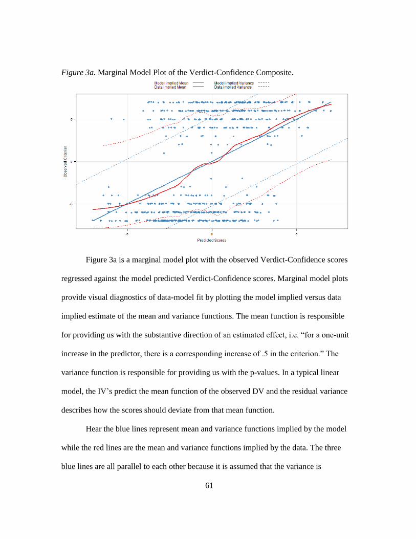
61
Figure 3a. Marginal Model Plot of the Verdict-Confidence Composite.
Figure 3a is a marginal model plot with the observed Verdict-Confidence scores
regressed against the model predicted Verdict-Confidence scores. Marginal model plots
provide visual diagnostics of data-model fit by plotting the model implied versus data
implied estimate of the mean and variance functions. The mean function is responsible
for providing us with the substantive direction of an estimated effect, i.e. “for a one-unit
increase in the predictor, there is a corresponding increase of .5 in the criterion.” The
variance function is responsible for providing us with the p-values. In a typical linear
model, the IV’s predict the mean function of the observed DV and the residual variance
describes how the scores should deviate from that mean function.
Hear the blue lines represent mean and variance functions implied by the model
while the red lines are the mean and variance functions implied by the data. The three
blue lines are all parallel to each other because it is assumed that the variance is

62
homogenous across the entirety of the mean function. Thus, the dashed blue lines visually
represent the homogeneity of variance assumption. Ideally, all the red lines should track
along all of the blue lines with little deviation beyond some random fluctuations.
In figure 3a, however, it is clear that both the mean function and more so the
variance function are misspecified. The model appears to overpredict scores below zero
and underpredict scores above zero as you can see in the deviations of the between the
solid red and blue lines. More importantly, the variance function shows a clear
pathological misfit with the data implied versus model implied variance functions never
even aligning. The fact that the red dashed lines are further away from the mean function
than the blue lines suggests that the model implied variance is too small. As such, the
standard errors for the significance tests will be too small, producing alpha inflation.
To give a sense of where that pathological misfit might be coming from it is
useful to compare the figure 3a, to figure 4a where the binary verdict has been incorrectly
analyzed as being continuous.

63
Figure 4a. Marginal Model Plot of the Binary Verdict.
In figure 4a, there is a somewhat more pronounced misfit in the mean function but
more importantly the plot retains the familiar pathological misfit in the variance function
as seen in figure 3a. Methodologists already know from logistic regression that assuming
normality with a binary DV produces incorrectly small standard errors.
It is also possible to visually inspect the severity of misfit in the variance function
direct with non-constant variance plot (also referred to as a spread level plot). Figure 5a
provides a plot for the verdict strength DV. Here we see that the linear non-constant
variance is only slightly off horizontal, but the non-linear non-constant variance severely
departs from zero. This is strong evidence for there being severe misspecification in the
variance function and that the tests of significance will be incorrect.

64
Figure 5a. Non-Constant Variance Plot for the Verdict-Confidence Composite.
Figure 6a. Non-Constant Variance Plot for the Binary Verdict.
To provide a comparison again, figure 6a is the non-constant variance plot for the
misspecified model where the binary verdict is being used with the similar x-shaped
spread appearing.

65
This is why I stated in the beginning that any perceived increase in statistical
power is illusory. What is happening is that the standard errors for the Verdict-
Confidence composite are consistently underestimated. This is because the composite is
being strongly influenced by the binary nature of verdict, as evident in how little
deviation there is from that binary nature in the composite (-7 and 7 are the most frequent
values, see figure 1a).
Figure 7a. QQ Plot of the Studentized Residuals of Verdict Strength
Note: The 95% confidence band was formed from 2000 replications of a
parametric bootstrap. The solid blue reference line runs through the quartiles of the two
distributions while the solid red line is drawn by robust regression. Robust regression is
designed to be robust to outliers and other influential points.
Deviations between the two lines provide evidence for the location of influential
outlying points. In this case, it is clear that the residuals both above and below the mean

66
of zero have some moderately strong outlying points as evidenced by the reference line
being offset the robust line at zero.
For all of this diagnostic investigation running a Monte Carlo simulation study
would be the best way to show that the Verdict-Confidence DV produces alpha inflation.
I think the simplest simulation study would require generating data with a covariance
matrix where all three variables (the binary IV, the binary Verdict, and the continuous
Confidence Rating) are all unrelated to each other. In addition to the covariance matrix,
I’d also need to specify the mean or threshold structure for the variables. Normally the IV
would be given a threshold value (e.g. .5) that would produce about equally sized groups.
Similarly, the Verdict variable could be given the same threshold value as the IV to
produce a roughly symmetric binary Verdict DV. The continuous Confidence Rating
variable could just be given a mean of 0 and standard deviation of 1. In this part, all that
remains would be to determine the sample size for the simulated datasets. Mplus could
handle this part (the data generation step) but it don’t believe I’d be able to use it to
analyze the simulation runs. I’d probably need to use something like R to manage the
analysis step.
Once data is simulated, the point could be made by analyzing the data with
normal theory standard errors and report the rate of alpha inflation. Now it might be
worth analyzing the data using a few different approaches to compare the rate of alpha
inflation in normal theory standard errors versus robust s.e. and bootstrapped s.e. It would
also be trivial to run the same analysis step on the same data with just the binary verdict.
I suspect, however, that this simple simulation study would still raise a few
questions about what happens at different sample sizes from the one we chose. If I choose
67
an n=40 (roughly 20 per condition) some might say that’s too small but if we choose an
n=500 others might say it is too big. Thus, I may then need to vary the sample size
parameter from very small to very big.
I can also imagine the following sets of complaints. People might take issue with
there being no correlation between the verdict and confidence rating variables. It would
be interesting to see if the size or direction of the correlation alters the rate of alpha
inflation. People might also take issue with the fact that verdict is equally split, as
departures from a 50:50 split produce alpha inflation. That is, what happens to the alpha
inflation of the Verdict-Confidence DV when verdict has an 80:20 split? Similarly, what
happens to alpha inflation when the confidence rating variable is skewed to the high end
or the low end?
In addition to all of these questions, you might also wonder if the Verdict-
Confidence DV results in under or over estimation of "real" effects. If the IV has a
moderate effect (in Cohen’s D terms) on verdict but no effect on confidence rating, what
happens to the estimated effect of the IV when you use the Verdict-Confidence DV?
Here’s where the correlation between verdict and confidence might make a difference
because if confidence is negatively correlated with verdict you could see something weird
like a sign reversal of the effect.
There’s also the open question of how to analyze the verdict and confidence
DV’s. I think a reasonable research question is "do the factors that influence confidence
ratings vary depending on the verdict rendered?" In my mind, you could answer that kind
of question in Mplus using a latent class model. You could define two latent classes using
the verdict DV and ask whether the IVs, demographic variables, or personality measures

68
predict confidence ratings within each of the two verdict groups (and test their equality
across the two classes). Moreover, if you wanted to make it slightly more interesting, you
could use the same model and now predict class membership along with confidence
ratings within class. In this model, you could have something like evidence strength
predicting class membership and moral foundations theory predicting confidence. Note:
this analysis would likely need a huge sample size, some strong simplifying assumptions,
or both.

69
APPENDIX B
MPLUS SYNTAX

70
Chapter 1
Title: Chapter 1 Model 0
Data: File is "searleD.txt";
Variable: Names are
juror
juryid
lc !Liberal to conservative
delib !1|Delib 2|NonDelib
case !1|Weak 2|Mod evidence
unitary !1|Unitary 2|Bifurcated
networth !1|High 2|low D$$
ivliab !1|P 2|D
IVliabR !1|P -1|D
jconf !Juror Confidence in Verdict
vcDV !Verdict-Confidence Composite
strevid !Juror rating of the evidence
boydgood boyddish
boydself !Primary Mediator
boygree boydtrus boydbeli boydeasy
;
Usevariables are
boydself
vcDV
;
Missing are .;
IDVARIABLE IS juror;
CLUSTER is juryid;
USEOBSERVATIONS are
delib EQ 1
;
Analysis:
TYPE IS Twolevel Basic;
estimator = mlr;
processors = 3;
Plot:
Type = plot3;

71
Chapter 2
Title: Model for the Counterfactual Effect
Data: File is "searleD.txt";
Usevariables are
boydself
vcDV
case
xm
;
USEOBSERVATIONS are
delib EQ 2
;
Define:
case = case - 1;
boydself = boydself - 4.603;
xm = case * boydself;
Analysis:
TYPE IS General;
estimator = ml;
BOOTSTRAP = 5000;
processors = 3;
Model:
boydself on case (a);
vcDV on boydself (b)
case (cp)
xm@0;
MODEL INDIRECT:
vcDV MOD boydself xm case;
Plot:
Type = plot3;
!OUTLIERS ARE LOGLIKELIHOOD INFLUENCE COOKS;
Save:
!FILE IS model0.txt;
Output:
cinterval(BCBOOTSTRAP)
sampstat stdyx;

72
Title: Model for the Counterfactual Effect with XM Interaction
Data: File is "searleD.txt";
Usevariables are
boydself
vcDV
case
xm
;
Missing are .;
IDVARIABLE IS juror;
USEOBSERVATIONS are
delib EQ 2
;
Define:
case = case - 1;
boydself = boydself - 4.603;
xm = case * boydself;
Analysis:
TYPE IS General;
estimator = ml;
BOOTSTRAP = 5000;
processors = 3;
Model:
boydself on case (a);
vcDV on boydself (b)
case (cp)
xm;
MODEL INDIRECT:
vcDV MOD boydself xm case;
Plot:
Type = plot3;
!OUTLIERS ARE LOGLIKELIHOOD INFLUENCE COOKS;
Save:
!FILE IS model0.txt;
Output:
cinterval(BCBOOTSTRAP)
sampstat stdyx;

73
Chapter 3
Title: Model for 2-2-2 Mediation Analysis
Data: File is "searleD.txt";
Usevariables are
boydself
vcDV
case
aggBS
;
Missing are .;
Within = boydself;
Between = aggBS case;
IDVARIABLE IS juror;
CLUSTER is juryid;
USEOBSERVATIONS are
delib EQ 1
;
Define:
aggBS = CLUSTER_MEAN (boydself);
CENTER aggBS (grandmean);
CENTER boydself (groupmean);
case = case - 1;
Analysis:
TYPE IS Twolevel;
estimator = mlr;
processors = 3;
Model:
%within%
vcDV on boydself;
%between%
aggBS on case (a);
vcDV on aggBS (b);
vcDV on case (cp);
Model Constraint:
New(ab);
ab = a*b;
Plot:
Type = plot3;
Output:
sampstat stdyx
cinterval(SYMMETRIC);

74
Chapter 5
Title: Full Model using the Counterfactually Defined Effects
Data: File is "searleD.txt";
Usevariables are
boydself
vcDV
case
aggBS
;
Within = boydself;
Between = aggBS case;
USEOBSERVATIONS are
delib EQ 1
;
Define:
aggBS = CLUSTER_MEAN (boydself);
CENTER aggBS boydself (grandmean);
case = case - 1; !To dummy code Case as 0,1
Analysis:
TYPE IS Twolevel;
estimator = mlr;
processors = 3;
Model:
%within%
vcDV on boydself (b1);
boydself;
%between%
aggBS on case (a);
vcDV on aggBS (b2);
vcDV on case (cp);
Model Constraint:
New(ab1 ab2 b3 ab3);
ab1 = a*b1; !a1b1 | within only
ab2 = a*b2; !a1b2 | contextual effect
b3 = b1 + b2; !between only effect
ab3 = a*b3; !a2b3 | pure level-2 effect
Plot:
Type = plot3;
Output:
sampstat stdyx cinterval(SYMMETRIC);

75
APPENDIX C
ICC, DESIGN EFFECTS, AND EFFECTIVE N
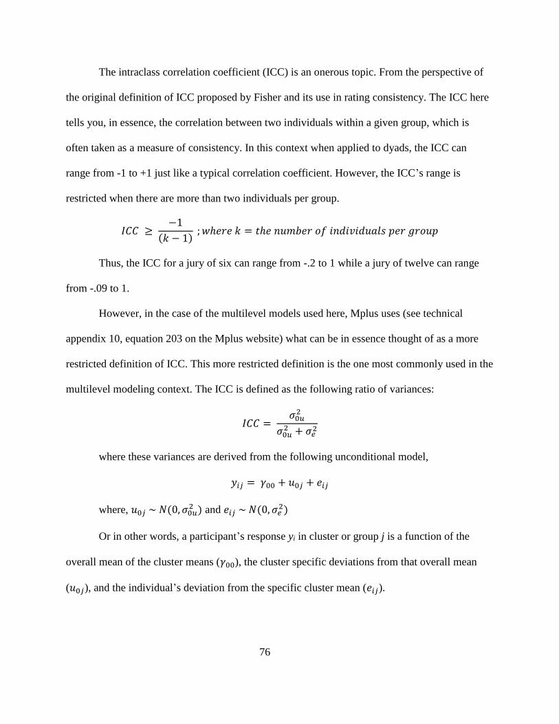
76
The intraclass correlation coefficient (ICC) is an onerous topic. From the perspective of
the original definition of ICC proposed by Fisher and its use in rating consistency. The ICC here
tells you, in essence, the correlation between two individuals within a given group, which is
often taken as a measure of consistency. In this context when applied to dyads, the ICC can
range from -1 to +1 just like a typical correlation coefficient. However, the ICC’s range is
restricted when there are more than two individuals per group.
𝐼𝐶𝐶 ≥ −1
(𝑘 − 1) ; 𝑤ℎ𝑒𝑟𝑒 𝑘 = 𝑡ℎ𝑒 𝑛𝑢𝑚𝑏𝑒𝑟 𝑜𝑓 𝑖𝑛𝑑𝑖𝑣𝑖𝑑𝑢𝑎𝑙𝑠 𝑝𝑒𝑟 𝑔𝑟𝑜𝑢𝑝
Thus, the ICC for a jury of six can range from -.2 to 1 while a jury of twelve can range
from -.09 to 1.
However, in the case of the multilevel models used here, Mplus uses (see technical
appendix 10, equation 203 on the Mplus website) what can be in essence thought of as a more
restricted definition of ICC. This more restricted definition is the one most commonly used in the
multilevel modeling context. The ICC is defined as the following ratio of variances:
𝐼𝐶𝐶 = 𝜎0𝑢
2
𝜎0𝑢2 + 𝜎𝑒
2
where these variances are derived from the following unconditional model,
𝑦𝑖𝑗 = 𝛾00 + 𝑢0𝑗 + 𝑒𝑖𝑗
where, 𝑢0𝑗 ~ 𝑁(0, 𝜎0𝑢2 ) and 𝑒𝑖𝑗 ~ 𝑁(0, 𝜎𝑒
2)
Or in other words, a participant’s response yi in cluster or group j is a function of the
overall mean of the cluster means (𝛾00), the cluster specific deviations from that overall mean
(𝑢0𝑗), and the individual’s deviation from the specific cluster mean (𝑒𝑖𝑗).

77
In the model, 𝑢0𝑗 and 𝑒𝑖𝑗 are both assumed to be normally distributed with a mean of zero
and some unknown variance (𝜎0𝑢2 and 𝜎𝑒
2, respectively). Given the definition of ICC above, an
appropriate interpretation of the ICC in this context is as the proportion of variance in the DV
that is accounted for by the differences between clusters. Here an ICC close to one would
suggest that most of the differences in Y across participants comes from differences in the
clusters, while an ICC close to zero would suggest that most of the differences in Y across
participants comes from individual differences. Because this is a ratio of variances it is
impossible for this ICC to be less than zero.
So what does this mean practically? If the researcher were to use interventions designed
to increase group polarization, they could produce negative ICCs which will result in model’s
crashing and failing to converge.
Design Effects and Effect N
Wholly separate from the issue of estimating the ICC, is the effect that an ICC has on the
standard errors and significance tests. One of the fundamental assumptions of regression is that
observations are independent of one another. This assumption is violated when there is clustering
in the data as measured by the ICC. It is possible to estimate the effect clustering has by using
the design effect to estimate the effective N.
𝐷𝑒𝑠𝑖𝑔𝑛 𝐸𝑓𝑓𝑒𝑐𝑡 = 1 + 𝐼𝐶𝐶 ∗ (𝑚 − 1); 𝑤ℎ𝑒𝑟𝑒 𝑚 = 𝑎𝑣𝑒𝑟𝑎𝑔𝑒 𝑐𝑙𝑢𝑠𝑡𝑒𝑟 𝑠𝑖𝑧𝑒
𝐸𝑓𝑓𝑒𝑐𝑡𝑖𝑣𝑒 𝑁 = 𝑛
𝐷𝑒𝑠𝑖𝑔𝑛 𝐸𝑓𝑓𝑒𝑐𝑡; 𝑤ℎ𝑒𝑟𝑒 𝑛 = 𝑠𝑎𝑚𝑝𝑙𝑒 𝑠𝑖𝑧𝑒
This is why for the Ruva study critiqued in chapter 1 if the ICC equals .38, then the
reported sample size of 320 goes to an effective sample size of just 120.


![Bayesian Causal Inference - uni-muenchen.de...from causal inference have been attracting much interest recently. [HHH18] propose that causal [HHH18] propose that causal inference stands](https://img.pdfslide.net/doc/110x75/5ec457b21b32702dbe2c9d4c/bayesian-causal-inference-uni-from-causal-inference-have-been-attracting.jpg)