Embed Size (px)
Citation preview
Politecnico di TorinoFacoltà di Ingegneria I
Corso di Laurea in Ingegneria Matematica
King Abdullah University of Science and TechnologyCenter for Uncertainty Quantification in Computational Science and Engineering
Master Thesis
Multilevel Monte Carlo method for PDEswith fluid dynamic applications
Advisor:
Prof. Claudio CANUTO
Co-advisor:
Dr. Matteo ICARDI
Co-advisor:
Prof. Raúl TEMPONECandidate:
Nathan QUADRIO
October 2014

Prof. Claudio Canuto
Department of Mathematics,
Polytechnic University of Turin,
Turin, Italy.
Dr. Matteo Icardi
Division of Mathematics & Computer, Electrical and Mathematical Sciences & Engineering
King Abdullah University of Science and Technology,
Thuwal, Kingdom of Saudi Arabia.
Prof. Raúl Tempone
Division of Mathematics & Computer, Electrical and Mathematical Sciences & Engineering
King Abdullah University of Science and Technology,
Thuwal, Kingdom of Saudi Arabia.
1

To Anita,
a light for me when all the other lights went out.
2

“In mathematics you don’t understand things. You just get used to them.”
John von Neumann
3
Abstract
This thesis focuses on PDEs in which some of the parameters are not known exactly but affected
by a certain amount of uncertainty, and hence described in terms of random variables/random
fields. This situation is quite common in engineering applications.
A common goal in this framework is to compute statistical indices, like mean or variance,
for some quantities of interest related to the solution of the equation at hand (“uncertainty
quantification"). The main challenge in this task is represented by the fact that in many appli-
cations tens/hundreds of random variables may be necessary to obtain an accurate represen-
tation of the solution variability. The numerical schemes adopted to perform the uncertainty
quantification should then be designed to reduce the degradation of their performance when-
ever the number of parameters increases, a phenomenon known as “curse of dimensionality".
A method that acts in this direction is Monte Carlo sampling. Such method is known to
be dimension independent and very robust but it is also known for is very slow convergence
rate. In this work we describe Monte Carlo sampling together with a solid error analysis and
we provide a test for its robustness by integrating different functions with different regularitues
and by solving different PDE problems with random coefficients.
Later on we introduce the technique of variance reduction and a further application of this
idea that goes with the name of Multilevel Monte Carlo (MLMC) method. The asymptotic cost
of solving the stochastic problem with the multilevel method is proved to be significantly lower
than that of the standard method and, in certain circumstances, grows only proportionally with
respect to the cost of solving the deterministic problem. Numerical calculations demonstrat-
ing its effectiveness are presented and more complex problems such as elliptic PDEs in a do-
main with random geometry are also presented, this last task has been performed to test a
code designed for the simulation of flow through porous media at the pore scale. The results
are promising considering the very complex geometries that require extremely expensive dis-
cretizations.
This work is the final outcome of the participation to the Visiting Student Research Pro-
gram at the King Abdullah University of Science and Technology, a project that allows students
4

to conduct research with faculty mentors in selected areas of pure and applied sciences, and a
Visiting Research Fellowship at the University of Texas in Austin.
Keywords: Uncertainty Quantification, Monte Carlo Sampling, Variance Reduction, Multi-
level Monte Carlo.
5

Acknowledgements
This thesis is the result of the fruitful collaboration among many people, who deserve grateful
acknowledgement.
My deepest thanks goes to Matteo Icardi for the huge support in every aspect of this work,
from the inspiring discussions at the blackboard to the technical guidance and suggestions in
the numerical results, to the proof-reading of every single page and slide I have written, with
24/7 availability.
A huge thanks goes also to Raúl Tempone: in addition to the warm hospitality in the many
places I have visited him and the contagious enthusiasm in facing any mathematical challenge,
I always have greatly benefitted from his help in discussing and dissecting any problem we had
to solve and from his many suggestions.
I am also greatly thankful to Claudio Canuto, who is and will always be a great inspiration
for me an my work, for the overall help and the infinite patience.
At KAUST, I would like to thank David Yeh, who made for me the whole KAUST experience
possible and great.
This thesis would not have been possible without the amazing and constant support I got
from my beloved ones: my parents, my grandma and my sister. The grand finale is however
for Anita, who is my love, my strength, my hope and my change of perspective. This thesis is
dedicated to her.
Turin, October 2014 Nathan Quadrio
6
Contents
Abstract 5
Acknowledgements 6
1 Introduction to Uncertainty Quantification 12
1.1 Forward uncertainty propagation . . . . . . . . . . . . . . . . . . . . . . . . . . . . 14
1.2 Inverse problem within uncertainty quantification . . . . . . . . . . . . . . . . . . 16
1.3 Overview . . . . . . . . . . . . . . . . . . . . . . . . . . . . . . . . . . . . . . . . . . . 19
2 Monte Carlo Method 20
2.1 Introduction . . . . . . . . . . . . . . . . . . . . . . . . . . . . . . . . . . . . . . . . . 20
2.2 Monte Carlo method . . . . . . . . . . . . . . . . . . . . . . . . . . . . . . . . . . . . 21
2.2.1 Numerical tests . . . . . . . . . . . . . . . . . . . . . . . . . . . . . . . . . . . 25
2.3 Quasi-Monte Carlo method . . . . . . . . . . . . . . . . . . . . . . . . . . . . . . . . 28
2.3.1 Error analysis in 1D . . . . . . . . . . . . . . . . . . . . . . . . . . . . . . . . . 30
2.3.2 Numerical tests . . . . . . . . . . . . . . . . . . . . . . . . . . . . . . . . . . . 32
2.4 Monte Carlo method for PDEs with random coefficient . . . . . . . . . . . . . . . 34
2.4.1 Error analysis . . . . . . . . . . . . . . . . . . . . . . . . . . . . . . . . . . . . 34
2.4.2 Complexity analysis . . . . . . . . . . . . . . . . . . . . . . . . . . . . . . . . 38
2.4.3 Numerical tests . . . . . . . . . . . . . . . . . . . . . . . . . . . . . . . . . . . 39
2.5 Variance Reduction . . . . . . . . . . . . . . . . . . . . . . . . . . . . . . . . . . . . . 44
2.5.1 Control Variate . . . . . . . . . . . . . . . . . . . . . . . . . . . . . . . . . . . 44
7
CONTENTS
3 Multilevel Monte Carlo Method 47
3.1 Introduction . . . . . . . . . . . . . . . . . . . . . . . . . . . . . . . . . . . . . . . . . 47
3.2 Multilevel Monte Carlo method . . . . . . . . . . . . . . . . . . . . . . . . . . . . . . 48
3.2.1 MLMC implementation . . . . . . . . . . . . . . . . . . . . . . . . . . . . . . 51
3.3 Numerical tests . . . . . . . . . . . . . . . . . . . . . . . . . . . . . . . . . . . . . . . 53
3.4 Application to random geometry problems . . . . . . . . . . . . . . . . . . . . . . . 56
3.4.1 Heterogeneous materials . . . . . . . . . . . . . . . . . . . . . . . . . . . . . 56
3.4.2 The geometry generation . . . . . . . . . . . . . . . . . . . . . . . . . . . . . 58
3.5 Simulations . . . . . . . . . . . . . . . . . . . . . . . . . . . . . . . . . . . . . . . . . 61
3.5.1 Elliptic PDE with random forcing . . . . . . . . . . . . . . . . . . . . . . . . 61
3.5.2 Elliptic PDE with a single random inclusion . . . . . . . . . . . . . . . . . . 63
3.5.3 Diffusion on a randomly perforated domain . . . . . . . . . . . . . . . . . . 66
3.5.4 Pore-scale Navier-Stokes . . . . . . . . . . . . . . . . . . . . . . . . . . . . . 68
3.6 Conclusions . . . . . . . . . . . . . . . . . . . . . . . . . . . . . . . . . . . . . . . . . 72
APPENDIX 72
A Multilevel Monte Carlo Pore-Scale Code 73
A.1 Main purpose . . . . . . . . . . . . . . . . . . . . . . . . . . . . . . . . . . . . . . . . 74
A.2 Structure . . . . . . . . . . . . . . . . . . . . . . . . . . . . . . . . . . . . . . . . . . . 74
A.3 Final statements . . . . . . . . . . . . . . . . . . . . . . . . . . . . . . . . . . . . . . . 76
8

List of Figures
1.1 Forward uncertainty propagation. . . . . . . . . . . . . . . . . . . . . . . . . . . . . 15
1.2 Bayesian inverse problem. . . . . . . . . . . . . . . . . . . . . . . . . . . . . . . . . . 16
1.3 Uncertainty quantification in bayesian inversion. . . . . . . . . . . . . . . . . . . . 18
2.1 Deterministic quadrature (left) vs. Monte Carlo sampled (right) points in the case
d = 2. . . . . . . . . . . . . . . . . . . . . . . . . . . . . . . . . . . . . . . . . . . . . . 23
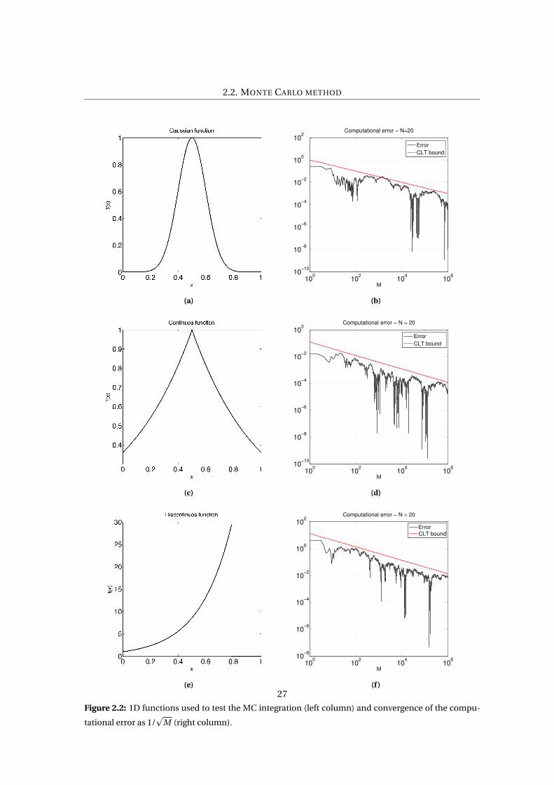
2.2 1D functions used to test the MC integration (left column) and convergence of
the computational error as 1/p
M (right column). . . . . . . . . . . . . . . . . . . . 27
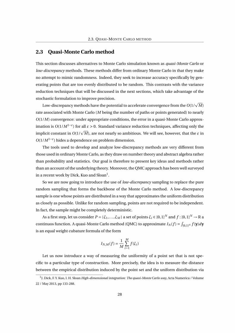
2.3 Idea of discrepancy (left) and example of Sobol sequence (right) in a two-dimensional
domain. The discrepancy can be also seen more intuitively as∆P = # points in [0,x]M −
Vol([0,x]). . . . . . . . . . . . . . . . . . . . . . . . . . . . . . . . . . . . . . . . . . . . 29
2.4 1D functions used to test the MC integration (left column) and convergence of the
computational error (right column) as 1/p
M for the MC and 1/M for the “good
cases” of QMC. . . . . . . . . . . . . . . . . . . . . . . . . . . . . . . . . . . . . . . . 33
2.5 Numerical simulation for Model 1 - Mesh refinement (left column, I = 1/h =64,128,512) and increase of the variability (right column N = 128,256,512). The
phenomenon of homogenization can be seen very well in the second column. . . 42
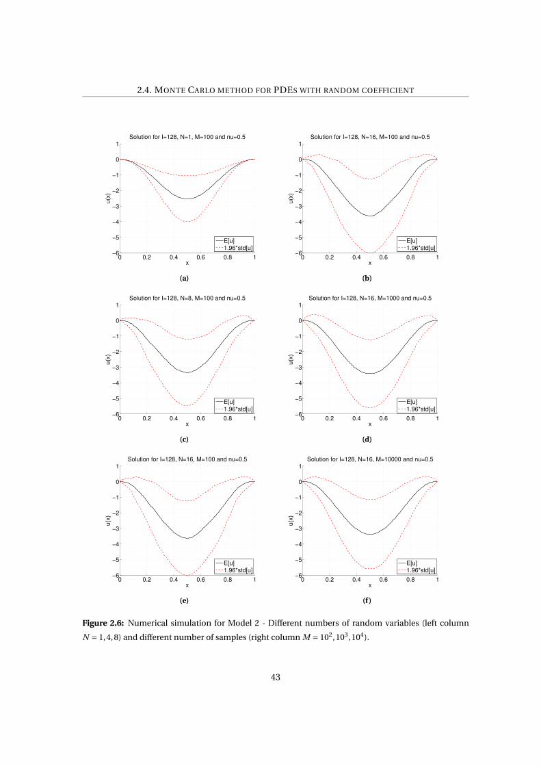
2.6 Numerical simulation for Model 2 - Different numbers of random variables (left
column N = 1,4,8) and different number of samples (right column M = 102,103,104). 43
9
LIST OF FIGURES
3.1 Numerical result for the 1D elliptic PDE with random diffusion solved modeled
with a piecewise constant coefficient. Rates of strong and weak error (up-left and
up-right plots resp.), consistency check (Eq. 3.3) and kurtosis (middle-left and
middle-right plots resp.), accuracy vs. cost (low-right) and sample vs. level for
different accuracies (low-left). . . . . . . . . . . . . . . . . . . . . . . . . . . . . . . 55
3.2 Examples of random heterogeneous materials. Left panel: A colloidal system of
hard spheres of two different sizes. Right panel: A Fontainebleau sandstone. Im-
ages from [37]. . . . . . . . . . . . . . . . . . . . . . . . . . . . . . . . . . . . . . . . . 57
3.3 Random geometry realizations. . . . . . . . . . . . . . . . . . . . . . . . . . . . . . . 59
3.4 Results for the QoI in the elliptic PDE with random forcing. . . . . . . . . . . . . . 61
3.5 Results for the QoI in the elliptic PDE with random forcing - γ estimate . . . . . . 62
3.6 Results for the elliptic PDE with a single random inclusion. . . . . . . . . . . . . . 63
3.7 Results for the elliptic PDE with a single random inclusion. . . . . . . . . . . . . . 64
3.8 Results for the diffusion on a randomly perforated domain. . . . . . . . . . . . . . 67
3.9 Mesh of a geometry realization. . . . . . . . . . . . . . . . . . . . . . . . . . . . . . . 69
3.10 Results for the incompressible Navier-Stokes flow simulation.. . . . . . . . . . . . 70
A.1 Pore-Scale Code. . . . . . . . . . . . . . . . . . . . . . . . . . . . . . . . . . . . . . . 73
10
List of Tables
3.1 Numerical result for the 1D elliptic PDE with random diffusion solved modeled
with a piecewise constant coefficient. . . . . . . . . . . . . . . . . . . . . . . . . . . 54
3.2 Cost comparison between MLMC and StdMC as ε→ 0 for the 1D elliptic PDE with
random diffusion. . . . . . . . . . . . . . . . . . . . . . . . . . . . . . . . . . . . . . . 54
3.3 Different classes of steady-state effective media problems considered here. F ∝KeG , where Ke is the general effective property, G is the average (or applied) gen-
eralized gradient or intensity field, and F is the average generalized flux field.
Class A and B problems share many common features and hence may be attacked
using similar techniques. Class C and D problems are similarly related to one an-
other. . . . . . . . . . . . . . . . . . . . . . . . . . . . . . . . . . . . . . . . . . . . . . 58
3.4 Results for the elliptic PDE with random forcing. . . . . . . . . . . . . . . . . . . . 63
3.5 Results for the diffusion in a random domain. . . . . . . . . . . . . . . . . . . . . . 66
3.6 Results for the incompressible Navier-Stokes flow simulation. . . . . . . . . . . . 71
3.7 Predicted cost of the MLMC estimator given by Theorem 4 to achieve a MSE of ε2
compared to the cost of the standard MC estimator given by Equation 2.4. . . . . 72
11

CHAPTER 1
Introduction to Uncertainty Quantification
Since more and more powerful computer are being developed, allowing for more complex
models to be solved, it is important to assess if the mathematical and the computational mod-
els are accurate enough and, in general, if one can establish an ”error bar” on the results or a
more accurate quantification of its variability. Uncertainty Quantification (UQ) aims at devel-
oping rigorous methods to characterize the impact of ”limited knowledge” on model parame-
ters of the quantities of interest. As UQ is at the interface of physics, mathematics and statistics,
a deep understanding of the physical problem of interest is required as well as its mathematical
description and a good probabilistic framework. In fact the most modern UQ approaches are a
combination of numerical analysis and statistical techniques.
Even if numerical simulations have reached a wide spread use and success in terms of low-
ering production costs and of reduction of physical prototyping, it still remains difficult to pro-
vide a certain confidence level in all the information obtained from numerical predictions. This
difficulty mainly comes from the amount of uncertainties related to the inputs of any compu-
tation attempting to represent a physical system. As a consequence, for some applications we
still prefer the physical tests, so that the quantification of the errors and uncertainties becomes
necessary in order to establish the numerical simulations predictive capabilities.
Classically, the errors leading to discrepancies between simulations and real world systems
are grouped into three distinct families:
• Model error: Simulations rely on the resolution of mathematical models taking into ac-
12
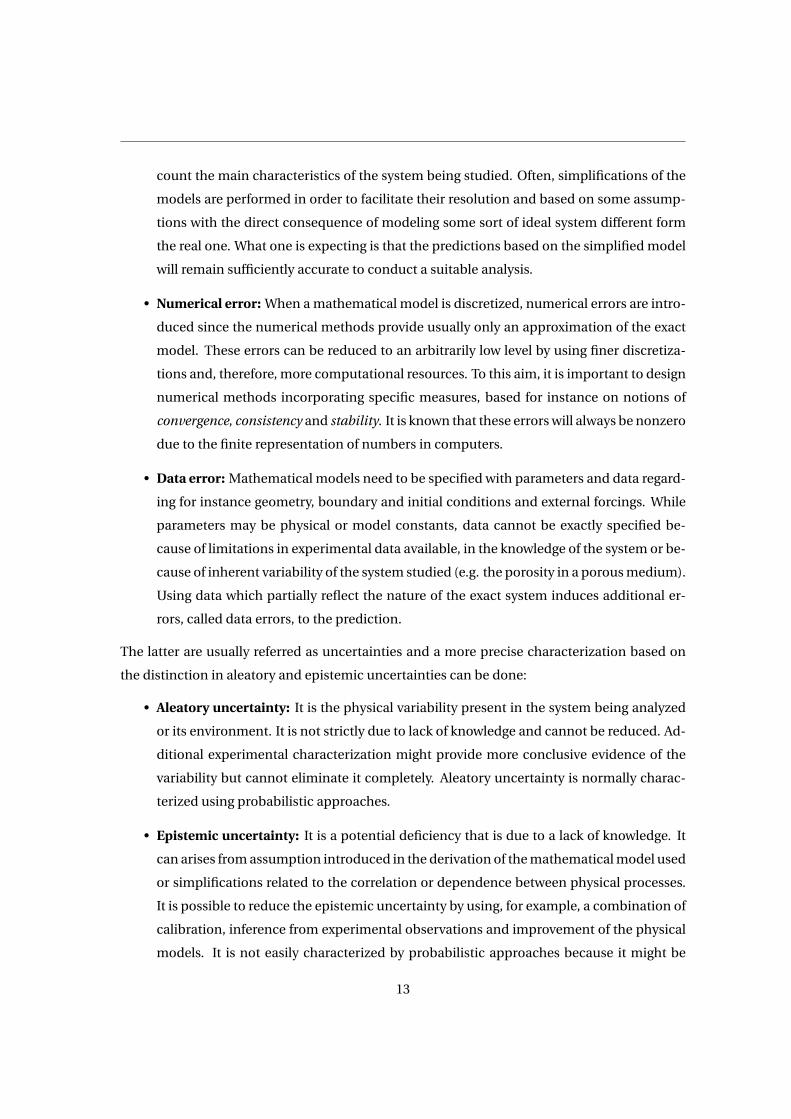
count the main characteristics of the system being studied. Often, simplifications of the
models are performed in order to facilitate their resolution and based on some assump-
tions with the direct consequence of modeling some sort of ideal system different form
the real one. What one is expecting is that the predictions based on the simplified model
will remain sufficiently accurate to conduct a suitable analysis.
• Numerical error: When a mathematical model is discretized, numerical errors are intro-
duced since the numerical methods provide usually only an approximation of the exact
model. These errors can be reduced to an arbitrarily low level by using finer discretiza-
tions and, therefore, more computational resources. To this aim, it is important to design
numerical methods incorporating specific measures, based for instance on notions of
convergence, consistency and stability. It is known that these errors will always be nonzero
due to the finite representation of numbers in computers.
• Data error: Mathematical models need to be specified with parameters and data regard-
ing for instance geometry, boundary and initial conditions and external forcings. While
parameters may be physical or model constants, data cannot be exactly specified be-
cause of limitations in experimental data available, in the knowledge of the system or be-
cause of inherent variability of the system studied (e.g. the porosity in a porous medium).
Using data which partially reflect the nature of the exact system induces additional er-
rors, called data errors, to the prediction.
The latter are usually referred as uncertainties and a more precise characterization based on
the distinction in aleatory and epistemic uncertainties can be done:
• Aleatory uncertainty: It is the physical variability present in the system being analyzed
or its environment. It is not strictly due to lack of knowledge and cannot be reduced. Ad-
ditional experimental characterization might provide more conclusive evidence of the
variability but cannot eliminate it completely. Aleatory uncertainty is normally charac-
terized using probabilistic approaches.
• Epistemic uncertainty: It is a potential deficiency that is due to a lack of knowledge. It
can arises from assumption introduced in the derivation of the mathematical model used
or simplifications related to the correlation or dependence between physical processes.
It is possible to reduce the epistemic uncertainty by using, for example, a combination of
calibration, inference from experimental observations and improvement of the physical
models. It is not easily characterized by probabilistic approaches because it might be
13
1.1. FORWARD UNCERTAINTY PROPAGATION
difficult to infer any statistical information due to the nominal lack of knowledge. Typical
examples of sources of epistemic uncertainties are turbulence model assumptions and
surrogate chemical kinetics models.
To sum up, what uncertainty analysis aims to is identifying the overall output uncertainty in a
given system.
There are two major types of problems in uncertainty quantification: one is the forward
propagation of uncertainty and the other is the inverse assessment of model uncertainty and
parameter uncertainty. There has been a proliferation of research on the former problem and
a number of numerical analysis techniques were developed for it. On the other hand, the lat-
ter problem is drawing increasing attention in the engineering design community, since un-
certainty quantification of a model and the subsequence predictions of the true system re-
sponse(s) are of great interest in both robust design and engineering design making.
1.1 Forward uncertainty propagation
Once a suitable mathematical model of a physical system is formulated, the numerically sim-
ulation task typically involves several steps.
Initially one has to specify the case, i.e. the input parameters. Generally, one needs to
state exactly the geometry associated with the system and, in particular, the computational
domain. Boundary conditions have also to be imposed. In the case of transient systems, ini-
tial conditions are also provided and, when present, external forcing functions are applied to
the system. In the end physical constants are also specified in order to describe the properties
of the system, as well as modeling or calibration data. The next step is the simulation. One
has to define a computational grid on which the model solution is first discretized. Additional
parameters related to time integration, whenever relevant, are also specified. Numerical so-
lution of the resulting discrete analogue of the mathematical model can then be performed.
Here one should choose a deterministic numerical model having a well-posed mathematical
formulation in the sense of Hadamard, i.e. one wants that the mathematical model admits the
existence of a unique solution with continuos dependence from the data, and with which can
be achieved small discretization errors. The final step concerns the analysis of the computed
solution.
The simulation methodology above reflects an idealized situation that may not be always
achieved in practice. In fact, in many cases, the input data set may not be completely known
due to the reasons mentioned before. Thus, though model equations may be deterministic,
14
1.1. FORWARD UNCERTAINTY PROPAGATION
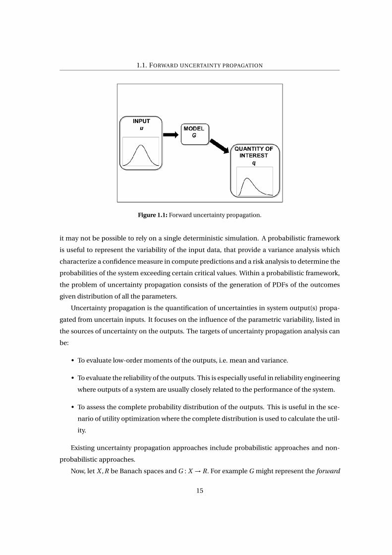
Figure 1.1: Forward uncertainty propagation.
it may not be possible to rely on a single deterministic simulation. A probabilistic framework
is useful to represent the variability of the input data, that provide a variance analysis which
characterize a confidence measure in compute predictions and a risk analysis to determine the
probabilities of the system exceeding certain critical values. Within a probabilistic framework,
the problem of uncertainty propagation consists of the generation of PDFs of the outcomes
given distribution of all the parameters.
Uncertainty propagation is the quantification of uncertainties in system output(s) propa-
gated from uncertain inputs. It focuses on the influence of the parametric variability, listed in
the sources of uncertainty on the outputs. The targets of uncertainty propagation analysis can
be:
• To evaluate low-order moments of the outputs, i.e. mean and variance.
• To evaluate the reliability of the outputs. This is especially useful in reliability engineering
where outputs of a system are usually closely related to the performance of the system.
• To assess the complete probability distribution of the outputs. This is useful in the sce-
nario of utility optimization where the complete distribution is used to calculate the util-
ity.
Existing uncertainty propagation approaches include probabilistic approaches and non-
probabilistic approaches.
Now, let X ,R be Banach spaces and G : X → R. For example G might represent the forward
15
1.2. INVERSE PROBLEM WITHIN UNCERTAINTY QUANTIFICATION
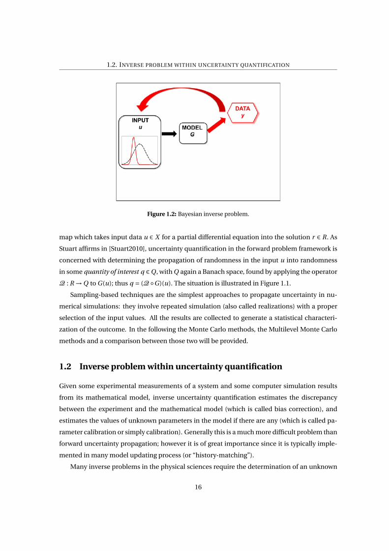
Figure 1.2: Bayesian inverse problem.
map which takes input data u ∈ X for a partial differential equation into the solution r ∈ R. As
Stuart affirms in [Stuart2010], uncertainty quantification in the forward problem framework is
concerned with determining the propagation of randomness in the input u into randomness
in some quantity of interest q ∈Q, with Q again a Banach space, found by applying the operator
Q : R →Q to G(u); thus q = (Q ◦G)(u). The situation is illustrated in Figure 1.1.
Sampling-based techniques are the simplest approaches to propagate uncertainty in nu-
merical simulations: they involve repeated simulation (also called realizations) with a proper
selection of the input values. All the results are collected to generate a statistical characteri-
zation of the outcome. In the following the Monte Carlo methods, the Multilevel Monte Carlo
methods and a comparison between those two will be provided.
1.2 Inverse problem within uncertainty quantification
Given some experimental measurements of a system and some computer simulation results
from its mathematical model, inverse uncertainty quantification estimates the discrepancy
between the experiment and the mathematical model (which is called bias correction), and
estimates the values of unknown parameters in the model if there are any (which is called pa-
rameter calibration or simply calibration). Generally this is a much more difficult problem than
forward uncertainty propagation; however it is of great importance since it is typically imple-
mented in many model updating process (or “history-matching”).
Many inverse problems in the physical sciences require the determination of an unknown
16
1.2. INVERSE PROBLEM WITHIN UNCERTAINTY QUANTIFICATION
field from a finite set of indirect measurements. Examples include oceanography, oil recov-
ery, water resource management and weather forecasting. In the Bayesian approach to these
problems, the unknown and the data are modelled as a jointly varying random variable, typi-
cally linked through solution of a partial differential equation, and the solution of the inverse
problem is the distribution of the unknown given the data.
Many important results and a lot of work has been done in this field, amongst the most
useful is one known as Bayes’ theorem:
prob(X |Y , I ) = prob(Y |X , I )×prob(X , I )
prob(Y , I )(1.1)
The importance of this property to data analysis becomes apparent if we replace X and Y by
“input” (also denoted as u) and “data” (also denoted as y):
prob(input | data, I ) ∝ prob(data | input, I )×prob(input, I )
The power of Bayes’ theorem lies in the fact that it relates the quantity of interest, the probabil-
ity that the hypothesis is true given the data, to the term we have a better chance of being able
to assign, the probability that we would have observed the measured data if the hypothesis was
true.
The various terms in Bayes’ theorem have formal names. The quantity on the far right,
prob(input, I ), is called the prior probability; it represents our state of knowledge (or ignorance)
about the truth of the hypothesis before we have analysed the current data. This is modified by
the experimental measurements through the likelihood function, or prob(data | input, I ), and
yields the posterior probability, prob(input | data, I ), representing our state of knowledge about
the truth of the hypothesis in the light of the data. In a sense, Bayes’ theorem encapsulates the
process of learning. We should note, however, that the equality of Eqn 1.1 has been replaced
with a proportionality, because the term prob(data|I ) (the so-called evidence) has been omit-
ted.
This approach is a natural way to provide estimates of the unknown field, together with
a quantification of the uncertainty associated with the estimate. It is hence a useful practi-
cal modelling tool. However it also provides a very elegant mathematical framework for in-
verse problems: whilst the classical approach to inverse problems leads to ill-posedness, the
Bayesian approach leads to a natural well-posedness and stability theory. Furthermore this
framework provides a way of deriving and developing algorithms which are well-suited to the
formidable computational challenges which arise from the conjunction of approximations aris-
ing from the numerical analysis of partial differential equations.
17
1.2. INVERSE PROBLEM WITHIN UNCERTAINTY QUANTIFICATION
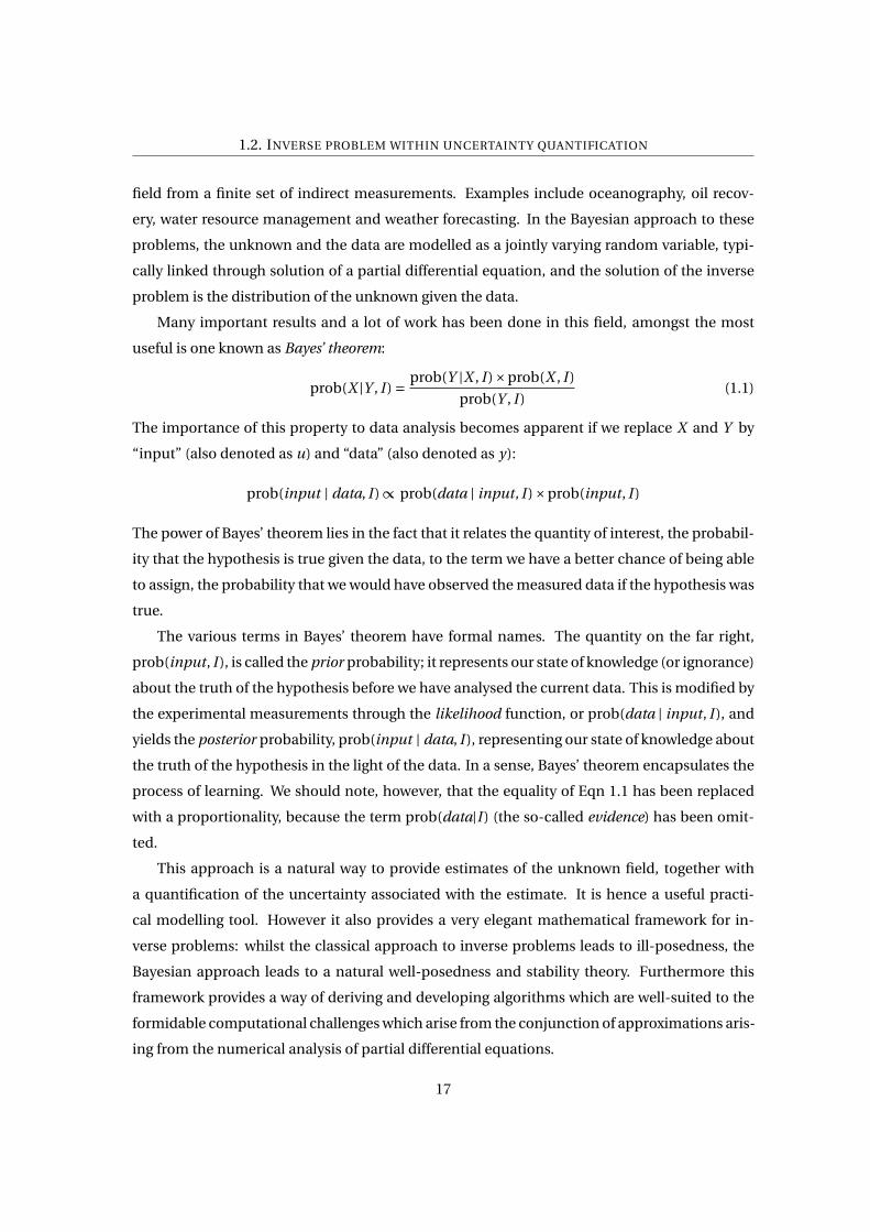
Figure 1.3: Uncertainty quantification in bayesian inversion.
So, in practice, inverse problems are concerned with the problem of determining the input
u when given noisy observed data y found from G(u). Let Y be the Banach space where the
observations lie, let O : R → Y denote the observation operator, define G = O ◦G , and consider
the equation
y =G (u)+η (1.2)
viewed as an equation for u ∈ X given y ∈ Y . The element η ∈ Y represents noise and typically
something about the size of η is known but the actual instance of η entering the data y is not
known. The aim is to reconstruct u from y. The Bayesian inverse problem is to find the condi-
tional probability distribution on u|y from the joint distribution of the random variable (u, y);
the latter is determined by specifying the distributions on u and η and, for example, assuming
that u and η are independent. This situation is illustrated in Figure 1.2.
To formulate the inverse problem probabilistically it is natural to work with separable Ba-
nach spaces as this allows for development of an integration theory as well as avoiding a variety
of pathologies that might otherwise arise; we assume separability from now on. The probabil-
ity measure on u is termed the prior, and will be denoted by µ0, and that on u|y the posterior,
and will be denoted by µy . Once the Bayesian inverse problems has been solved, the uncer-
tainty in q can be quantified with respect to input distributed according to the posterior on
u|y, resulting in improved quantification of uncertainty in comparison with simply using in-
put distributed according to the prior on u. The situation is illustrated in Figure 1.3. The black
dotted lines demonstrate uncertainty quantification prior to incorporating the data, the red
18
1.3. OVERVIEW
curves demonstrate uncertainty quantification after the data has been incorporated by means
of Bayesian inversion.
1.3 Overview
This thesis consists in four chapters and it illustrates methods that could be applicable in both
forward and inverse problem frameworks.
In Chapter 2, for the sake of generality we introduce the Monte Carlo and Quasi-Monte
Carlo method in the context of high-dimensional integration. We show the robustness of the
former and the convenience of the latter in terms of convergence rate. Then we show the ap-
plication of Monte Carlo in the PDEs framework and we provide the relative error analysis. In
the end, we introduce another Monte Carlo improving technique, the variance reduction one,
which gives the idea that lies behind the main argument of this thesis.
In Chapter 3, we show a clever variance reduction technique, the Giles’ multilevel Monte
Carlo. The theory is provided together with some simple tests cases to show its effectiveness
and its convenience in terms of computational costs. In the end we also provide some appli-
cations in Computational Fluid Dynamic problems, in particular we provide the results of the
simulation of PDEs on a random geometry. So, if in a first instance we deal with PDEs with
random coefficient coming from a Karhunen-Loève expansion or from a piecewise constant
model in the second one we try to apply the same methodologies to a different kind of random
parameter.
19
CHAPTER 2
Monte Carlo Method
2.1 Introduction
In this chapter we first review the Monte Carlo and the quasi-Monte Carlo method in the con-
text of high-dimensional integration. Then we show the application of Monte Carlo in PDE with
random coefficients and, after some error analysis, we provide and comment some numerical
tests with their results.
The Monte Carlo method is a widely used tool in many disciplines, including physics, chem-
istry, engineering, finance, biology, computer graphics, operations research and management
science. Examples of problems that it can address are:
• A call center manager wants to know if adding a certain number of service representative
during peak hours would help decrease the waiting time of calling customers.
• A portfolio manager needs to determine the magnitude of the loss in value that could
occur with a 1% probability over a one-week period.
• The designer of telecommunications network needs to make sure that the probability of
losing information cells in the network is below a certain thresold.
Realistic models of the system above typically assume that at least some of their components
behave in a random way. For instance, the call arrival times and processing times for the call
center cannot realistically be assumed to be fixed and known ahead of time and thus it makes
sense instead to assume that they occur according to some stochastic model.
20
2.2. MONTE CARLO METHOD
The Monte Carlo simulation method uses random sampling to study properties of systems
with components that behave in a random fashion. More precisely, the idea is to simulate on
the computer the behavior of these systems by randomly generating the variables describing
the behavior of their components. Samples of the quantities of interest can then be obtained
and used for statistical inference.
2.2 Monte Carlo method
The Monte Carlo method is certainly very popular and its origins can be traced back in 1946,
when physicists at Los Alamos Scientific Laboratory were investigating radiation shielding and
the distance that neutrons would likely travel through various materials. Despite having most
of the necessary data, such as the average distance a neutron would travel in a substance be-
fore it collided with an atomic nucleus, and how much energy the neutron was likely to give off
following a collision, the Los Alamos physicists were unable to solve the problem using con-
ventional, deterministic mathematical methods. Stanislaw Ulam had the idea of using random
experiments. He recounts his inspiration when he was convalescing from an illness and play-
ing solitaires. He questioned himself on the chances that the cards of a Canfield solitaire can
come out successfully. After spending a lot of time trying to estimate them by pure combi-
natorial calculations, he wondered whether a more practical method than “abstract thinking”
might not be to lay it out say one hundred times and simply observe and count the number of
successful plays. This was already possible to envisage with the beginning of the new era of fast
computers, and he immediately thought of problems of neutron diffusion and other questions
of mathematical physics, and more generally how to change processes described by certain
differential equations into an equivalent form interpretable as a succession of random opera-
tions. Later in 1946, he described the idea to John von Neumann and they began to plan actual
calculations.
Being secret, the work of von Neumann and Ulam required a code name. Von Neumann
chose the name Monte Carlo. The name refers to the Monte Carlo Casino in Monaco where
Ulam’s uncle would borrow money to gamble. Using lists of "truly random" random numbers
was extremely slow, but von Neumann developed a way to calculate pseudorandom numbers,
using the middle-square method. Though this method has been criticized as crude, von Neu-
mann was aware of this: he justified it as being faster than any other method at his disposal,
and also noted that when it went awry it did so obviously, unlike methods that could be subtly
incorrect.
21
2.2. MONTE CARLO METHOD
Monte Carlo methods were central to the simulations required for the Manhattan Project,
though severely limited by the computational tools at the time. In the 1950s they were used
at Los Alamos for early work relating to the development of the hydrogen bomb, and became
popularized in the fields of physics, physical chemistry, and operations research. The Rand
Corporation and the U.S. Air Force were two of the major organizations responsible for funding
and disseminating information on Monte Carlo methods during this time, and they began to
find a wide application in many different fields.
So, the fundamental idea on which Monte Carlo (MC) methods rely is a pseudo-random
sampling of a RV in order to construct a set of realization of the input data. To each of these
realizations corresponds a unique solution of the model.
In many stochastic applications one wants to estimate E [Y ] . In standard MC approach one
can simulate it using
A (Y ; M) ≡ 1
M
M∑i=1
Y (ωi ),
ωi being independent and identically distributed (iid) samples, and choose M sufficiently large
to control the statistical error
E [Y ]−A (Y ; M)
The following example of Monte Carlo integration will be more clarifying than any other expla-
nations.
Example The integral I = ∫[0,1]N f (x)dx will be computed by the Monte Carlo method, where it
is assumed f (x) : [0,1]N →R. Let Y = f (X ), where X is uniformly distributed in [0,1]N . One has:
I =∫
[0,1]Nf (x)d x
=∫
[0,1]Nf (x)p(x)d x [p is the uniform pdf]
= E[
f (x)]
[x is uniformly distributed in [0,1]N ]
' 1
M
M∑i=1
f (x(ω(i )))
≡ IN ,M
where the values {x(ω j )} are iid and are sampled uniformly in the cube [0,1]d by sampling the
components xi (ω j ) independently and uniformly on the interval [0,1]. We can find an example
on how the evaluation points are taken in Figure 2.1, where we can see the difference between a
Monte Carlo quadrature against a deterministic one (uniform).
22
2.2. MONTE CARLO METHOD
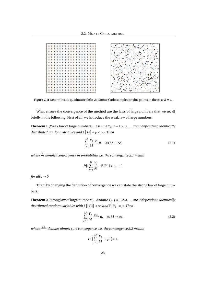
Figure 2.1: Deterministic quadrature (left) vs. Monte Carlo sampled (right) points in the case d = 2.
What ensure the convergence of the method are the laws of large numbers that we recall
briefly in the following. First of all, we introduce the weak law of large numbers.
Theorem 1 (Weak law of large numbers). Assume Y j , j = 1,2,3, . . . are independent, identically
distributed random variables and E[Y j
]=µ<∞. Then
M∑j=1
Y j
MP−→µ, as M →∞, (2.1)
whereP−→ denotes convergence in probability, i.e. the convergence 2.1 means
P(| M∑
j=1
Y j
M−E [Y ] | > ε)→ 0
for all ε→ 0
Then, by changing the definition of convergence we can state the strong law of large num-
bers.
Theorem 2 (Strong law of large numbers). Assume Y j , j = 1,2,3, . . . are independent, identically
distributed random variables with E[|Y j |
]<∞ and E[Y j
]=µ. Then
M∑j=1
Y j
Ma.s.−−→µ, as M →∞, (2.2)
wherea.s.−−→ denotes almost sure convergence, i.e. the convergence 2.2 means
P({ M∑
j=1
Y j
M→µ
})= 1.
23
2.2. MONTE CARLO METHOD
In other words, the important result that lies behind the Laws of Large Numbers is that a for
large M the empirical average is very close to the expected value µ with very high probability.
Now that we know for sure that the method converge to something, we would like to say
something about the rate of convergence. To understand this and how the statistical error be-
have we can refer to the Central Limit Theorem that now will be also recalled.
Theorem 3. Assume ξ j , j = 1,2,3, . . . are independent, identically distributed (iid) and E[ξ j
]= 0,
E[ξ2
j
]= 1. Then
M∑j=1
ξ jpM
* ν,
where ν is N (0,1) and* denotes convergence of the distributions, also called weak convergence,
i.e. the convergence means
E
[g( M∑
j=1
ξ jpM
)]→ E
[g (ν)
],
for all bounded and continuous functions g .
Having this in mind and referring to the example, one can compute the error IM − I to see
in practice how this theorem can be applied in the MC context.
Let the error εM be defined by
εM =M∑
j=1
f (x j )
M−
∫[0,1]d
f (x)d x
=M∑
j=1
f (x j )−M E[
f (x)]
M
By the Central Limit Theorem, one has
pMεM *σν,
where ν is N (0,1) and
σ2 =∫
[0,1]df 2(x)d x −
(∫[0,1]d
f (x)d x)2
=∫
[0,1]d
(f 2(x)−
∫[0,1]d
f (x)d x)2
d x
In practice, σ2 is approximated by
σ2 = 1
M −1
M∑j=1
(f (x j )−
M∑m=1
f (xm)
M
)
24
2.2. MONTE CARLO METHOD
This implies that for any set B = (−C ,C )
P (p
MεM ∈ B) → P (N (0,1) ∈ B)
Given a constant, 0 <α¿ 1, one has to choose C =Cα such that the following confidence level
constraint is satisfied
P (N (0,1) ∈ B) =∫|x|≤Cα
e−x2
2p2π
d x = 1−α
So in the end one has
P (|εM | ≤ CαpM
) ≈ 1−α, for large M
Hence the statistical error of the Monte Carlo estimator is O(1/p
M), which is independent
of the dimension d . The comparison between the convergence rate of a deterministic quadra-
ture, say M−2/d of the trapezoidal rule, versus M−1/2 supports the suggestion that, even for
moderate dimensions d , the Monte Carlo method can outperform deterministic methods.
Although the Monte Carlo error has the nice property that its convergence rate of 1/p
M
does not depend on the dimension, this rate is slow. For this reason, a lot of work has been done
to find ways of improving the Monte Carlo error and two different paths can be taken. The first
one is try to find ways of reducing the variance σ2 of f . Methods achieving this are under the
category of variance reduction techniques. The second approach is to use an alternative sam-
pling mechanism (a deterministic one actually) - often called quasi-random or low-discrepancy
sampling - whose corresponding error has a better convergence rate. Using these alternative
sampling mechanisms for numerical integration is usually referred to as quasi-Monte Carlo in-
tegration.
2.2.1 Numerical tests
In this paragraph we show the results of some actual computations. The sources of these exer-
cises can be traced back at the summer school in Mathematical and Algorithmic aspects of
Uncertainty Quantification hold by Nobile and Tempone at the University of Texas, Austin.
Similarly to the very first example of the chapter, we are interested in calculating the follow-
ing quantity
g =∫
[0,1]Nf (x)dx
for some different functions that mainly differ by the degree of regularity. In particular we look
at different examples of f for some real constants {cn , wn }Nn=1 taken from
25
2.2. MONTE CARLO METHOD
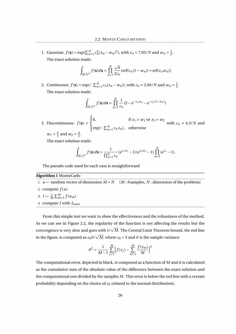
1. Gaussian: f (x) = exp(∑N
n=1 c2n(xn −wn)2), with cn = 7.03/N and wn = 1
2 .
The exact solution reads:∫[0,1]N
f (x)dx =N∏
n=1
pπ
2cn(erf(cn(1−wn))+erf(cn wn))
2. Continuous: f (x) = exp(−∑Nn=1 cn |xn −wn |), with cn = 2.04/N and wn = 1
2 .
The exact solution reads:∫[0,1]N
f (x)dx =N∏
n=1
1
cn(2−e−cn wn −e−cn (1−wn ))
3. Discontinuous: f (x) =
0, if x1 > w1 or x2 > w2
exp(−∑Nn=1 cn xn), otherwise
with cn = 4.3/N and
w1 = π4 and w2 = π
5 .
The exact solution reads:∫[0,1]N
f (x)dx = 1∏Nn=1 cn
(ec1w1 −1)(ec2w2 −1)N∏
n=3(ecn −1).
The pseudo code used for each case is straightforward
Algorithm 1 MonteCarlo
1: u ← random vector of dimension M ×N [M : #samples, N : dimension of the problem]
2: compute f (u)
3: I ← 1M
∑Mm=1 f (um)
4: compare I with Iexact
From this simple test we want to show the effectiveness and the robustness of the method.
As we can see in Figure 2.2, the regularity of the function is not affecting the results but the
convergence is very slow and goes with 1/p
M . The Central Limit Theorem bound, the red line
in the figure, is computed as c0σ/p
M , where c0 = 3 and σ is the sample variance
σ2 = 1
M −1
M∑j=1
(f (x j )−
M∑m=1
f (xm)
M
)2
The computational error, depicted in black, is computed as a function of M and it is calculated
as the cumulative sum of the absolute value of the difference between the exact solution and
the computational one divided by the samples M . This error is below the red line with a certain
probability depending on the choice of c0 (related to the normal distribution).
26
2.2. MONTE CARLO METHOD
(a)
100
102
104
106
10−10
10−8
10−6
10−4
10−2
100
102
Computational error − N=20
M
Error
CLT bound
(b)
(c)
100
102
104
106
10−10
10−8
10−6
10−4
10−2
100
Computational error − N = 20
M
Error
CLT bound
(d)
(e)
100
102
104
106
10−8
10−6
10−4
10−2
100
102
Computational error − N = 20
M
ErrorCLT bound
(f )
Figure 2.2: 1D functions used to test the MC integration (left column) and convergence of the compu-
tational error as 1/p
M (right column).
27
2.3. QUASI-MONTE CARLO METHOD
2.3 Quasi-Monte Carlo method
This section discusses alternatives to Monte Carlo simulation known as quasi-Monte Carlo or
low-discrepancy methods. These methods differ from ordinary Monte Carlo in that they make
no attempt to mimic randomness. Indeed, they seek to increase accuracy specifically by gen-
erating points that are too evenly distributed to be random. This contrasts with the variance
reduction techniques that will be discussed in the next sections, which take advantage of the
stochastic formulation to improve precision.
Low-discrepancy methods have the potential to accelerate convergence from the O(1/p
M)
rate associated with Monte Carlo (M being the number of paths or points generated) to nearly
O(1/M) convergence: under appropriate conditions, the error in a quasi-Monte Carlo approx-
imation is O(1/M 1−ε) for all ε > 0. Standard variance reduction techniques, affecting only the
implicit constant in O(1/p
M), are not nearly so ambitious. We will see, however, that the ε in
O(1/M 1−ε) hides a dependence on problem dimension.
The tools used to develop and analyze low-discrepancy methods are very different from
those used in ordinary Monte Carlo, as they draw on number theory and abstract algebra rather
than probability and statistics. Our goal is therefore to present key ideas and methods rather
than an account of the underlying theory. Moreover, the QMC approach has been well surveyed
in a recent work by Dick, Kuo and Sloan1.
So we are now going to introduce the use of low-discrepancy sampling to replace the pure
random sampling that forms the backbone of the Monte Carlo method. A low-discrepancy
sample is one whose points are distributed in a way that approximates the uniform distribution
as closely as possible. Unlike for random sampling, points are not required to be independent.
In fact, the sample might be completely deterministic.
As a first step, let us consider P = {ξ1, . . . ,ξM } a set of points ξi ∈ [0,1]N and f : [0,1]N →R a
continuos function. A quasi-Monte Carlo method (QMC) to approximate IN ( f ) = ∫[0,1]N f (y)dy
is an equal weight cubature formula of the form
IN ,M ( f ) = 1
M
M∑i=1
f (ξi )
Let us now introduce a way of measuring the uniformity of a point set that is not spe-
cific to a particular type of construction. More precisely, the idea is to measure the distance
between the empirical distribution induced by the point set and the uniform distribution via
1J. Dick, F. Y. Kuo, I. H. Sloan High-dimensional integration: The quasi-Monte Carlo way, Acta Numerica / Volume
22 / May 2013, pp 133-288.
28
2.3. QUASI-MONTE CARLO METHOD
the Kolmogorov-Smirnov statistic. The concept of discrepancy looks precisely at such distance
measures. We can then define it as
Definizione 1. Let x ∈ [0,1]N and [0,x] = [0, x1]×·· ·× [0, xN ], then the local discrepancy is
∆P (x) = 1
M
M∑i=1
1[0,x](ξi )−N∏
i=1xi
while the star-discrepancy is
∆∗P,N = sup
x∈[0,1]N|∆P (x)|
(a) Discrepancy. (b) Sobol sequence.
Figure 2.3: Idea of discrepancy (left) and example of Sobol sequence (right) in a two-dimensional do-
main. The discrepancy can be also seen more intuitively as ∆P = # points in [0,x]M −Vol([0,x]).
We can have a more intuitive idea of discrepancy by looking at Figure 2.3(a) and we can give
an alternative definition as
∆P = # points in [0,x]
M−Vol([0,x])
At this point we can introduce the definition of low discrepancy sequences.
Definizione 2. A sequence (ξ1,ξ2, . . . ), ξi ∈ [0,1]N is a low discrepancy sequence if the set of
points PM = (ξ1, . . . ,ξM ) satisfies
∆∗PM ,N ≤CN
(log M)N
M.
29
2.3. QUASI-MONTE CARLO METHOD
So we can say that QMC methods use equal weight cubature formulae with low discrep-
ancy sequences of points. Several sequences exist in literature, some of them available also in
MATLAB, such as: Halton, Hammersley, Sobol, Faure, Niederreiter, etc...
The simplest example is the Halton sequence and in order to construct that sequence we
first have to define the radical inverse function φb(i ) as follows:
if i =∞∑
n=1inbn−1, in ∈ {0,1, . . . ,b −1} , then φb(i ) =
∞∑n=1
inb−n ,
so, in base b = 10, the radical inverse of i = 15421 is φ10(i ) = 0.12451. Then, if p1, . . . , pN denote
the first N prime numbers, the Halton sequence P = {ξ1,ξ2, . . . } is given by
ξi = (φp1 (i ),φp2 (i ), . . . ,φpN (i ))
and its star-discrepancy satisfies
∆∗N := sup
x∈[0,1]N|∆P (x)| =O
( (log M)N
M
)Other better sequences instead such as Hammersley, Sobol, Faure, etc... have a star-discrepancy
∆∗N =O
( (log M)N−1
M
).
2.3.1 Error analysis in 1D
Let us consider for simplicity the N = 1 dimensional case just to have an idea on how the dis-
crepancy comes into play in this framework. The result can be generalized for arbitrary dimen-
sion. The following error representation holds:
1
M
M∑i=1
f (ξi )−∫
[0,1]f (y)d y =∆P (1) f (1)−
∫[0,1]
∆P (y) f ′(y)d y
which proof can be find in [Nobile,Tempone].
Hence, the error in the QMC integration is bounded by
∣∣∣ 1
M
M∑i=1
f (ξi )−∫
[0,1]f (y)d y
∣∣∣= ∣∣∣∫[0,1]
∆P (y) f ′(y)d y∣∣∣≤∆∗
P‖ f ′‖L1(0,1)
To estimate the error in practice in a quasi-Monte Carlo computation, the following strategy
has been adopted. We consider η∼U ([0,1]N ) as a uniformly distributed random vector (shift)
and
IN ,M ( f ,η) = 1
M
M∑i=1
f ({ξi +η })
30
2.3. QUASI-MONTE CARLO METHOD
as the QMC formula with the random shift η. Then we take s i.i.d. shifts η1, . . . ,ηs ∼U ([0,1]N ).
Finally we estimate the integral
IN ,M ( f ) = 1
s
s∑j=1
IN ,M ( f ,η j ) = 1
sM
s∑j=1
M∑i=1
f ({ξi +η j })
and the error based on the η−sample standard deviation, i.e.
eN ,M ( f ) = c0ps
√√√√ 1ps −1
s∑j=1
(IN ,M ( f ,η j )− IN ,M ( f ))2
In Figure 2.4 this quantity is represented with a green label. We can see that it gets more
and more precise as the number of shifts increase2.
2More details about these results can be found in [Nobile,Tempone].
31
2.3. QUASI-MONTE CARLO METHOD
2.3.2 Numerical tests
In this section we provide an estimation of the same integrals reported above with a quasi-
Monte Carlo method. We use the function i4_sobol_generate.m to generate Sobol sequences3.
The pseudocode for the algorithm is the following
Algorithm 2 Quasi Monte Carlo
1: U ← i4_sobol_generate(M , N ) [generate the Sobol sequence]
2: for i = 1 → S do
3: shift ← rand(N ,1), [generate the random vector of shifts]
4: ushift ← mod(U +SS,1) [compute a shifted sequence]
5: u ← [u,ushift] [update the overall vector of random points]
6: compute f (u)
7: I ← 1M ·S
∑M ·Sm=1 f (um)
8: compare I with Iexact
The Sobol sequence generator works on base 2 so the initial amount of sample is M = 2048.
Moreover, for the computation a number of shifts s = 1000 is chosen.
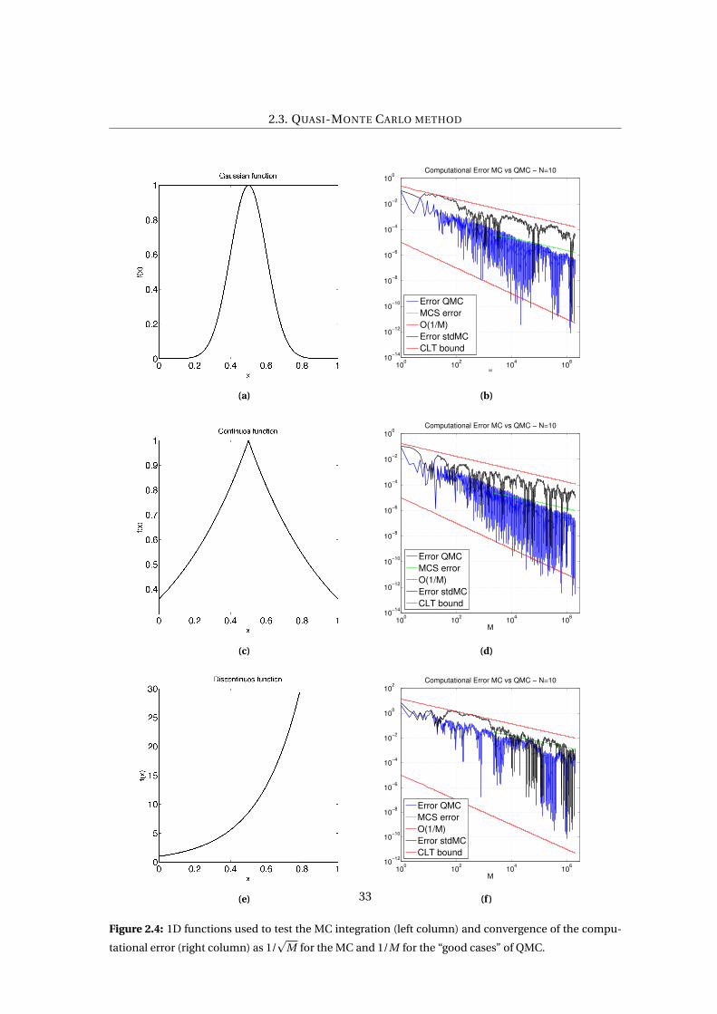
In Figure 2.4 we can see in the right column the behavior of the correspondent function
on the left. In the black line we indicate the standard Monte Carlo computational error as
we did in the previous section. in the blue line instead, we represent the Quasi-Monte Carlo
computational error. The red lines represent the two rates O(1/p
M) and O(1/M) while the
green one is the error based on the η−sample standard deviation. We were expecting the latter
to be above the QMC error with a certain probability related to the choice of c0, but as we can
see, is true only after a certain number of shifts.
It is clear how in this framework the methods does not behave in the same way for different
types of regularity of the integrand function. If in the case of a continuos or a infinitely differ-
entiable function we have a gain of the rate at almost O(1/M) in the case of the discontinuous
function instead remain pretty similar to the stdMC one.
3This package has been taken from John Burkardt’s home page:
http://people.sc.fsu.edu/∼jburkardt/m_src/m_src.html.
32
2.3. QUASI-MONTE CARLO METHOD
(a)
100
102
104
106
10−14
10−12
10−10
10−8
10−6
10−4
10−2
100
M
Computational Error MC vs QMC − N=10
Error QMC
MCS error
O(1/M)
Error stdMC
CLT bound
(b)
(c)
100
102
104
106
10−14
10−12
10−10
10−8
10−6
10−4
10−2
100
M
Computational Error MC vs QMC − N=10
Error QMC
MCS error
O(1/M)
Error stdMC
CLT bound
(d)
(e)
100
102
104
106
10−12
10−10
10−8
10−6
10−4
10−2
100
102
M
Computational Error MC vs QMC − N=10
Error QMC
MCS error
O(1/M)
Error stdMC
CLT bound
(f )
Figure 2.4: 1D functions used to test the MC integration (left column) and convergence of the compu-
tational error (right column) as 1/p
M for the MC and 1/M for the “good cases” of QMC.
33
2.4. MONTE CARLO METHOD FOR PDES WITH RANDOM COEFFICIENT
2.4 Monte Carlo method for PDEs with random coefficient
In this section we provide some numerical analysis to discuss the sources of error that occurs
when we deal with SPDEs and we try to solve the randomness with a sampling-based tech-
nique. We are going to define and denote u as the solution of a certain problem, y as the vector
of random parameters and we want to find the expectation of a certain quantity of interest Q
in order to place ourselves in the framework described in Chapter 1. The main results of this
analysis come from [32]. Here we develop some calculations and add some clarifications.
Let y = (y1, . . . , yN ) be a random vector with density ρ(y) : Γ→ R+, u(y) : Γ→ V a Hilbert-
valued function, u ∈ L2ρ(Γ;V ), and Q : V →R a continuous functional on V (possibly non linear),
such that E[|Q(u(y))|p]<∞ for p sufficiently large.
Similarly as before, the goal here is to compute E[Q(u(y))
]and using the classical Monte
Carlo approach one can approximate expectation by sample averages. In fact, if {y(ωm)}Mm=1 be
iid y samples one has
E[Q(u(y))
]≈ 1
M
M∑m=1
Q(u(y(ωm)))
where for each y(ωm) one has to find the solution u(y(ωm)) of the PDE and evaluate the q.o.i.
Q(u(y(ωm))). As said before, the Monte Carlo approach has the nice property that the con-
vergence rate is M−1/2 independently from the length of y and the regularity of u(.), but the
convergence is slow and, in this case, the possibly available regularity of the solution cannot be
exploited.
Assume now that the PDE had been discretized by some mean (finite elements, finite vol-
umes, spectral methods,...), so that in practice the discrete solutions uh(y(ωm)), m = 1, . . . , M
are computed. Then the MC estimator will be
E[Q(u(y))
]≈ 1
M
M∑m=1
Q(uh(y(ωm)))
2.4.1 Error analysis
At this point some error analysis can be done. The first thing that one can notice is that the
error is composed of two terms. In fact
E[Q(u(y))
]− 1
M
M∑m=1
Q(uh(y(ωm))) =
= E[Q(u(y))
]−E[Q(uh(y))
]+E[Q(uh(y))
]− 1
M
M∑m=1
Q(uh(y(ωm))) =
34
2.4. MONTE CARLO METHOD FOR PDES WITH RANDOM COEFFICIENT
= E[Q(u(y))−Q(uh(y))
]︸ ︷︷ ︸discretization error
+E[Q(uh(y))
]− 1
M
M∑m=1
Q(uh(y(ωm)))︸ ︷︷ ︸statistical error
where the first term is the discretization error that will be denoted as E Q (h) while the second is
the statistical error that will be denoted EQh (M).
Discretization error
Let Q : V →R with Q(0) = 0 be a functional that is globally Lipschitz, i.e.
∃CQ > 0 s.t. |Q(u)−Q(u′)| ≤CQ‖u −u′‖V , ∀u,u′ ∈V
and assume that exists α> 0 and Cu(y) > 0 with∫ΓCu(y)pρ(y)dy <∞ for some p > 1, such that
‖u(y)−uh(y)‖V ≤Cu(y)hα, ∀y ∈ Γ and 0 < h < h0 (2.3)
Then
|E Q (h)| = |E[Q(u(y))−Q(uh(y))
] | = |∫Γ
(Q(u(y))−Q(uh(y)))ρ(y)dy|
≤ CQ
∫Γ‖u(y)−uh(y)‖V ρ(y)dy
≤ CQ hα∫Γ
Cu(y)ρ(y)dy
≤ CQ‖Cu‖Lpρ
hα
The value of α in Equation 2.3 may depend both on the space V and on the accuracy order
of the approximation method chosen. Since in our application we take both piecewise linear
finite element method and first order accuracy finite volume methods and the space is usually
L2 the we are expecting α= 2.
Example Consider the following elliptic problem with uniformly bounded random coefficient−div(a(x,y)∇u(x,y)) = f (x), x ∈ D
u(x,y) = 0, x ∈ ∂D∀y ∈ Γ⊂RN
where D ⊂ Rd is an open, convex, Lipschitz domain and f ∈ L2(D). The assumptions on the
random coefficient are the following:
• finite Karhunen–Loève expansion: a(x,y) = a +∑Ni=1
√λi yi bi (x);
35
2.4. MONTE CARLO METHOD FOR PDES WITH RANDOM COEFFICIENT
• independence of the RVs: yi ∼U (−p3,p
3) iid (so Γ= [−p3,p
3]N );
• bi ∈C∞(D);
•∑N
i=1
√3λi‖bi‖∞ ≤ δa, 0 < δ< 1.
Thanks to these one can state the following
(1−δ)a ≤ a(x,y) ≤ (1+δ)a, ‖∇a(·,y)‖L∞(D) ≤Ca , ∀y ∈ Γ
that ensure the coercivity of the bilinear form. Moreover, denoting
H 10 = {v ∈ H 1(D) : ‖v −ϕn‖H 1(D) → 0, for some (ϕn) ⊂C∞
0 (D)}
endowed with the norm ||v ||H 10= ||∇v ||L2(D) and thanks to the Lax-Milgram theorem (see [7],
sect. 4.2) which is valid under these conditions, we can assert the existence, the uniqueness of the
solution u(y) ∈ H 10 ⊂ H 1(D) and the continuos dependency from the data
‖u(y)‖H 10 (D) ≤
CP‖ f ‖L2(D)
(1−δ)a, ∀y ∈ Γ
where CP is the Poincaré constant, i.e.
‖v‖L2(D) ≤CP‖v‖H 10 (D), v ∈ H 1
0 (D).
Moreover, since the problem is elliptic with homogenous boundary conditions, f ∈ L2 and the
domain is convex (see [8]), a uniform bound in y can be stated on the H 2−norm of the solution
∃Cu > 0, s.t. ‖u(y)‖H 2(D) ≤Cu , ∀y ∈ Γ
Since the problem is well-posed in the sense of Hadamard, one can state the weak formulation
and then consider a well-posed discrete formulation. Now in particular, a piecewise linear finite
element approximation will be taken in consideration so the problem can be written∀y ∈ Γ find uh(y) ∈Vh , s.t.∫D a(·,y)∇uh(y) ·∇vh(y) = ∫
D f vh ∀vh ∈Vh
where Vh ⊂ H 10 (D) is the space of continuous piecewise linear functions on a uniform and ad-
missible triangulation Th , vanishing on ∂D.
The discrete solution uh(y) satisfies the same bound as the continuous one,
||uh(y)||H 1(D) ≤|| f ||L2(D)
(1−δ)a√
1+C 2P
, ∀y ∈ Γ
36
2.4. MONTE CARLO METHOD FOR PDES WITH RANDOM COEFFICIENT
and
E[|Q(uh(y))|p] 1
p ≤ E[(CQ ||uh(y)||)p] 1
p ≤ CQ || f ||L2(D)
(1−δ)a√
1+C 2P
, ∀p ≥ 1
Then
||u(y)−uh(y)||L2(D) +h||∇u(y)−∇uh(y)||L2(D) ≤Cuh2
Since the bound is uniform in y, all moments are bounded
E[||u(y)−uh(y)||p
L2(D)
] 1p +hE
[||∇u(y)−∇uh(y)||p
L2(D)
] 1p ≤Cuh2, ∀p ≥ 1
Statistical error
Assuming that Q is a globally Lipschitz functional one can observe that
EQh (M) = E
[Q(uh(y))
]− 1
M
M∑m=1
Q(uh(y(ωm)))
= 1
M
M∑m=1
[E[Q(uh(y))
]−Q(uh(y(ωm)))]
and, if one takes the expectation with respect to the random sample,
E[E
Qh (M)
]= 0
Then
Var[E
Qh (M)
]= 1
MVar
[Q(uh(y))
]and one can estimate
Var[Q(uh(y))
] ≤ E[Q(uh(y))2]
≤ C 2Q ||uh ||2L2
ρ(Γ;V )
≤ 2C 2Q (||u||2
L2ρ(Γ;V )
+||u −uh ||2L2ρ(Γ;V )
)
≤ 2C 2Q (||u||2
L2ρ(Γ;V )
+h2α||Cu ||2L2ρ(Γ;V )
) <∞
In the end one can conclude that for Lipschitz functionals Q one has
Var[E
Qh (M)
]≤ C
M→ 0 as M →∞
with constant C uniformly bounded with respect to h. Moreover, since Var[Q(uh(y))
] ≤ C one
can apply the law of large numbers, law of iterated logarithms and the Central Limit Theorem.
In particular, the previous result implies, via the Chebyshev inequality, convergence in proba-
bility, that is, for any given ε> 0
P (|E Qh (M)| > ε) ≤
Var[E
Qh (M)
]ε2 ≤ C
Mε2 → 0 as M →∞
37
2.4. MONTE CARLO METHOD FOR PDES WITH RANDOM COEFFICIENT
2.4.2 Complexity analysis
In the end one has that the error can be split in two sources as
E[Q(u(y))
]− 1
M
M∑m=1
Q(uh(y(ωm))) = E Q (h)+EQh (M)
where
|E Q (h)| = |E[Q(u(y))−Q(uh(y))
] | ≤C hα
is the discretization error and
|E Qh (M)| = |E[
Q(uh(y))]− 1
M
M∑m=1
Q(uh(y(ωm)))| ≤C0
√Var[Q(uh)]
M
is the statistical error motivated by the Central Limit Theorem, i.e.
P (p
M |E Qh (M)| ≤ c0
√Var[Q(uh)]) → 2Φ(c0)−1 as M →∞
Let be assumed now that the computational work to solve for each u(y(ωm)) is O(h−dγ), where
d is the dimension of the computational domain and γ > 0 represents the complexity of gen-
erating one sample with respect to the number of degrees of freedom. One has therefore the
following estimates
W ∝ Mh−dγ
for the total work and
|E Q (h)|+ |E Qh (M)| ≤C1hα+ C2p
Mfor the total error. What one would like to do is to choose optimally h and M and one possible
way is to minimize the computational work subject to an accuracy constraint, i.e. the problem
can be written find minh,M Mh−dγ s.t.
C1hα+ C2pM
≤ TOL
The Lagrangian of the above problem is
L (M ,h,λ) = Mh−dγ+λ(C1hα+ C2pM
−TOL)
Therefore one gets to the system∂L∂M = h−dγ− λC2
2p
M 3= 0
∂L∂h =−dγMh−dγ−1 +λC1αhα−1 = 0
∂L∂λ =C1hα+ C2p
M−TOL = 0
38
2.4. MONTE CARLO METHOD FOR PDES WITH RANDOM COEFFICIENT
Taking in consideration the first and the second equation, resolving with respect to M and
eliminating λ one get to1pM
= 2αC1
dγC2hα
using the third equation and resolving with respect to h one has
C1hα+C22αC1
dγC2−TOL = 0
hα = TOLdγ
C1(dγ+2α)→ 1p
M= TOL
2α
C2(dγ+2α)
Since1pM
∝ TOL → M ∝ TOL−2
hα∝ TOL → h ∝ TOL1/α
the resulting complexity is then
W ∝ TOL−(2+dγ/α) (2.4)
2.4.3 Numerical tests
In this case we want to look at the solution of a one dimensional boundary value problem
−(a(x,ω)u′(x,ω))′ = 4π2 cos(2πx)︸ ︷︷ ︸=: f (x)
, for x ∈ (0,1)
with u(0, .) = u(1, .) = 0 and we are interested in computing the expected value of the following
QoI
Q(u(ω)) =∫ 1
0u(x,ω)d x
We use an uniform I +1 uniform grid 0 = x0 < x1 < <xI = 1 on [0,1] with uniform spacing h =xi −xi−1 = 1/I , i = 1, . . . , I . Using this grid we can build a piecewise linear FEM approximation,
uh(x,ω) =I−1∑i=1
uh,i (ω)ϕi (x),
yielding a tridiagonal linear system for the nodal values, A(ω)uh(ω) = F, with
Ai ,i−1(ω) =−a(xi−1/2,ω)
h2
Ai ,i (ω) = a(xi−1/2,ω)+a(xi+1/2,ω)
h2
39
2.4. MONTE CARLO METHOD FOR PDES WITH RANDOM COEFFICIENT
Ai ,i+1(ω) =−a(xi+1/2,ω)
h2
and
Fi = f (xi ).
Here we used the notation xi+1/2 = xi+xi+12 and xi−1/2 = xi+xi−1
2 . The integral in Q(uh) can be
then computed exactly by a trapezoidal method, yielding
Q(uh) = hI−1∑i=1
uh,i .
We look at two different models for the diffusion coefficient a(x,ω). The first is a piecewise
constant model and we define it as
a(x,ω) = 1+σN∑
n=1Yn(ω)I[xn−1,xn ](x),
with equispaced nodes xn = nN for 0 ≤ n ≤ N and i.i.d. uniform random variables Yn ∼U ([−p3,
p3]).
Tests are conducted for different uniform mesh refinements, i.e. values of I = N 2l , l ≥ 0. We also
try different number of input random variables N = 10, N = 20 and N = 40. The constant σ has
been chosen ensuring coercivity, namely 1−σp3 > 0.
The second model is defined as
a(x,ω) = exp(κ(x,ω))
where κ(x,ω) is a stationary random field with the Matérn covariance function
C (x, y) =σ2 1
Γ(ν)2ν−1
(p2ν
|x − y |ρ
)νKν
(p2ν
|x − y |ρ
)where Γ is the gamma function and Kν is the modified Bessel function of the second kind. We
look at the following special cases of C with ρ = 0.1 and σ2 = 2
ν= 0.5, C (x, y) = σ2 exp(−|x − y |
ρ
)ν= 1.5, C (x, y) = σ2
(1+
p3|x − y |ρ
)exp
(−p
3|x − y |ρ
)ν= 2.5, C (x, y) = σ2
(1+
p5|x − y |ρ
+p
3|x − y |2ρ2
)exp
(−p
5|x − y |ρ
)ν→∞, C (x, y) = σ2 exp
(−|x − y |2
2ρ2
)For this example we chose to represent the stationary random κ(x,ω) using the truncated
Karhunen-Loève expansion with N terms
κ(x,ω) ≈N∑
n=1
√λnYn(ω)en(x)
40
2.4. MONTE CARLO METHOD FOR PDES WITH RANDOM COEFFICIENT
where {Yk } is a set of i.i.d. uniform random variables over [−p3,p
3]. To find the eigenfunction
and eigenvalues of C we solve the eigenvalue problem∫ 1
0C (x, y)en(y)d y =λnen(x) (2.5)
we do this by discretizing C as a matrix by evaluating the function C (xi+ 12
, x j+ 12
) over the grid
{ xi+ 12
}I−1i=0
×{ xi+ 12
}I−1i=0
with N ≤ I . Then we use MATLAB’s function eig() and we place the eigen-
vector in a decreasing order, namely
λ1 <λ2 < ·· · <λN
This discretization corresponds to a piecewise constant FEM approximation to the eigenvalue
problem (2.5).
With the theory that lies behind the Karhunen-Loève expansion we could fill an entire sec-
tion. In this work we decided to avoid the explanations as we used it as a tool to develop our
calculations.
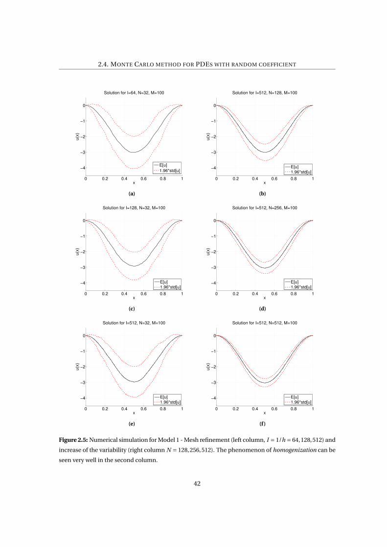
In Figure 2.5 we present the results related to Model 1. We decide to represent the expected
value of the solution (black line) in each point of the domain with the relative standard devi-
ation (red lines). We do that for different mesh refinements (left column) and for a different
number of random variables (right column), namely in the left column the refinements are
shown while in the right column the increasing random variables. The main result that we
want to point out is the homogenization of the random coefficient. This phenomenon consists
in a sort of averaging of the coefficient which can be approximated as a constant one better and
better as the number of random variables increases, that is as become more and more oscillat-
ing. It can be seen in the significant reduction of variance in the Figure 2.5(f). The conclusion
is that the estimate of our quantity of interest gets more and more accurate as the variability of
the problem increases.
In Figure 2.6 instead we present the results related to Model 2. Again, in black we repre-
sent the expected value of the solution in each point of the domain with the relative standard
deviation in red. In the left column we decided to test different truncations of the KL expan-
sion while keeping constant the mesh refinements. In the right column instead we present the
results with a different number of samples making sure to choose a number of terms of the
KL expansion that covers the 90% of the spectrum. In this case, unlike the previous case, we
can see that the more terms we include the more the variability of the problem increases until
we cover a reasonable part of the spectrum. On the other hand, if we increase the number of
samples, we can see the convergence of the standard deviation and, therefore, of the variance.
41
2.4. MONTE CARLO METHOD FOR PDES WITH RANDOM COEFFICIENT
0 0.2 0.4 0.6 0.8 1
−4
−3
−2
−1
0
Solution for I=64, N=32, M=100
x
u(x
)
E[u]
1.96*std[u]
(a)
0 0.2 0.4 0.6 0.8 1
−4
−3
−2
−1
0
Solution for I=512, N=128, M=100
x
u(x
)
E[u]1.96*std[u]
(b)
0 0.2 0.4 0.6 0.8 1
−4
−3
−2
−1
0
Solution for I=128, N=32, M=100
x
u(x
)
E[u]1.96*std[u]
(c)
0 0.2 0.4 0.6 0.8 1
−4
−3
−2
−1
0
Solution for I=512, N=256, M=100
x
u(x
)
E[u]1.96*std[u]
(d)
0 0.2 0.4 0.6 0.8 1
−4
−3
−2
−1
0
Solution for I=512, N=32, M=100
x
u(x
)
E[u]1.96*std[u]
(e)
0 0.2 0.4 0.6 0.8 1
−4
−3
−2
−1
0
Solution for I=512, N=512, M=100
x
u(x
)
E[u]1.96*std[u]
(f )
Figure 2.5: Numerical simulation for Model 1 - Mesh refinement (left column, I = 1/h = 64,128,512) and
increase of the variability (right column N = 128,256,512). The phenomenon of homogenization can be
seen very well in the second column.
42
2.4. MONTE CARLO METHOD FOR PDES WITH RANDOM COEFFICIENT
0 0.2 0.4 0.6 0.8 1−6
−5
−4
−3
−2
−1
0
1Solution for I=128, N=1, M=100 and nu=0.5
x
u(x
)
E[u]1.96*std[u]
(a)
0 0.2 0.4 0.6 0.8 1−6
−5
−4
−3
−2
−1
0
1Solution for I=128, N=16, M=100 and nu=0.5
x
u(x
)
E[u]1.96*std[u]
(b)
0 0.2 0.4 0.6 0.8 1−6
−5
−4
−3
−2
−1
0
1Solution for I=128, N=8, M=100 and nu=0.5
x
u(x
)
E[u]1.96*std[u]
(c)
0 0.2 0.4 0.6 0.8 1−6
−5
−4
−3
−2
−1
0
1Solution for I=128, N=16, M=1000 and nu=0.5
x
u(x
)
E[u]1.96*std[u]
(d)
0 0.2 0.4 0.6 0.8 1−6
−5
−4
−3
−2
−1
0
1Solution for I=128, N=16, M=100 and nu=0.5
x
u(x
)
E[u]1.96*std[u]
(e)
0 0.2 0.4 0.6 0.8 1−6
−5
−4
−3
−2
−1
0
1Solution for I=128, N=16, M=10000 and nu=0.5
x
u(x
)
E[u]1.96*std[u]
(f )
Figure 2.6: Numerical simulation for Model 2 - Different numbers of random variables (left column
N = 1,4,8) and different number of samples (right column M = 102,103,104).
43
2.5. VARIANCE REDUCTION
2.5 Variance Reduction
Since the Monte Carlo error can be written as
E [Y ]− 1
M
M∑j=1
Y (ω j ) ≈Cα
√Var[Y ]
M
the paths to reduce it that we can walk through are two: the first is to increase the samples M
while the other is reduce the quantity Var[Y ] . So the main idea of variance reduction is try to
“reduce” Var[Y ] without changing E [Y ] . In practice, one wants to find another RV Z such that:
• E [Z ] = E [Y ] ;
• Var[Z ] ¿ Var[Y ] ;
and then apply the Monte Carlo method to the variable Z instead of Y in a way that
E [Y ]− 1
M
M∑j=1
Z (ω j ) ≈Cα
√Var[Z ]
M¿Cα
√Var[Y ]
M.
2.5.1 Control Variate
In this case the idea is to look for a RV X that has a strong correlation (positive or negative) with
Y and a known mean E [X ] , generate a sample of both RVs and combine the empirical means
to an estimator with lower variance than the MC one.
Then, one can define a new random variable
Z (β) = Y −β(X −E [X ])
The point is that since since E [X ] is known, we are free to add a term β(X −E [X ]) with mean
zero to the MC estimator, so that the unbiasedness is preserved. The variance is:
Var[
Z (β)] = E
[(Y −β(X −E [X ])−E [Y ])2]
= E[((Y −E [Y ])−β(X −E [X ]))2]
= Var[Y ]+β2 Var[X ]−2βCov(X ,Y )
If one derives this last expression with respect to β, the minimum can be easily found to be
β∗ = Cov(X ,Y )
Var[X ]
44
2.5. VARIANCE REDUCTION
and one has a total variance reduction of
Var[
Z (β∗)]= Var[Y ]
(1− (Cov(X ,Y ))2
Var[X ]Var[Y ]
)< Var[Y ]
In practice, all the quantities are approximate using sample covariances and variances. It should
be pointed out that this kind of variance reduction really pays off under certain conditions, i.e.
if the assumption that the work to generate the pair (X j ,Y j ) is (1+θ) times the work to generate
Y j is made one has that this strategy is convenient only if
Var[Y ] > (1+θ)Var[V (β∗)
]then, we can remark the previous condition as
1 > (1+θ)(1−ρ2) → ρ2 > 1
1+θExample Consider Monte Carlo integration for calculating I = ∫ 1
0 f (x)d x. This integral can be
seen as the expected value of f (U ), where
f (x) = 1
1+x
and U follows a uniform distribution [0,1]. Using a sample of size M and denoting the sample
as u1, . . . ,uM , one has that the estimate is given by
I ≈ 1
M
M∑i=1
f (ui ).
If one introduces g (x) = 1+x as a control variate with a known expected value
E[g (U )
]= ∫ 1
0(1+x)d x = 3
2
can combine the two into a new estimate
I ≈ 1
M
M∑i=1
f (ui )− β∗( 1
M
M∑i=1
g (ui )− 3
2
)Using M = 5000, the following results has been obtained, where the coefficient β∗ has been esti-
Estimate Variance
Classical estimate 0.6952 0.0196
Control variate 0.6931 0.0006
45
2.5. VARIANCE REDUCTION
mated with the sample covariance and variance respectively
s f ,g = 1
M −1
M∑j=1
( f (u j )− 1
M
M∑i=1
f (ui ))(g (u j )− 1
M
M∑i=1
g (ui ))
sg = 1
M −1
M∑j=1
(g (u j )− 1
M
M∑i=1
g (ui ))2
so that β∗ ≈ 0.4768 and the variance has been reduced by 97%. Note that the exact result is ln2 ≈0.69314718
Although this example is very simple and intuitive, a few words must be spent on the kind of
control variables are typically used in practice. In theory, any variable X correlated with Y and
whose expectation is known can be used as a control variable. This means that the potential
candidates to be used are quantities that are closely related to the one for which we try to esti-
mate the mean, but that are, in some sense, simpler and whose expectation is known.
In the context of SPDE or PDE with random coefficient we can apply this idea using a
coarser discretization of the problem (e.g. with double the gridsize h) with the same realiza-
tion of {Yk } as a control variable for the approximation of E [Q(uh)]. This idea is the basis of
multilevel Monte Carlo and the results will be shown in the next chapter.
46
CHAPTER 3
Multilevel Monte Carlo Method
3.1 Introduction
Monte Carlo methods are a very general and useful approach to the estimation of quantities
arising from stochastic simulation. However they can be computationally expensive, partic-
ularly when the cost of generating individual stochastic samples is very high, as in the case
of stochastic PDEs. Multilevel Monte Carlo is a recently developed approach which greatly
reduces the computational cost by performing most simulations with low accuracy at a corre-
spondingly low cost, with relatively few simulations being performed at high accuracy and a
high cost.
According to [16], when the dimensionality of the uncertainty (or the uncertain input pa-
rameters) is low, it can be appropriately modeled using the Fokker-Planck PDE (when is the Eu-
lerian counterpart of an SDE) and using stochastic Galerkin, stochastic collocation or polyno-
mial chaos methods (Xiu and Karniadakis 2002, Babuška, Tempone and Zouraris 2004, Babuška,
Nobile and Tempone 2010, Gunzburger, Webster and Zhang 2014). When the level of uncer-
tainty is low, and its effect is largely linear, then moment methods can be an efficient and accu-
rate way in which to quantify the effects on uncertainty (Putko, Taylor, Newman and Green
2002). However, when the uncertainty is high-dimensional and strongly non-linear, Monte
Carlo simulation remains the preferred approach.
Monte Carlo simulation is extremely simple as we could appreciate in the previous chapters
and we already know that its weakness relies in its computational cost that can be very high,
47
3.2. MULTILEVEL MONTE CARLO METHOD
particularly when when each sample might require the approximate solution of a PDE, or a
computation with many time steps.
Giles and Waterhouse in [17] developed a variant of MLMC which uses quasi-Monte Carlo
samples instead of independent Monte Carlo samples. The numerical results were very en-
couraging for SDE applications in which the dominant computational cost was on the coarsest
levels of resolution where QMC is known to be most effective due to the low number of dimen-
sions involved. However there was no supporting theory for this research.
More recently, there has been considerable research on the theoretical foundations for
multilevel QMC (MLQMC) methods (Niu, Hickernell, Müller-Gronbach and Ritter 2010, Kuo,
Schwab and Sloan 2012, Dick et al. 2013, Baldeaux and Gnewuch 2014, Dick and Gnewuch
2014a, Dick and Gnewuch 2014b). These theoretical developments are very encouraging, and
may lead to the development of new, more efficient, multilevel methods.
3.2 Multilevel Monte Carlo method
The history of multilevel Monte Carlo can be traced back to Heinrich et al. [21, 22], where it
was introduced in the context of parametric integration. Kebaier [23] then used similar ideas
for a two-level Monte Carlo method to approximate weak solutions to stochastic differential
equations in mathematical finance. As we have already seen, one of the classic approaches to
Monte Carlo variance reduction is through the use of a control variate which is well correlated
with the variable we want to approximate and has a known expectation. In [15], Giles extended
this idea to more that two levels and dubbed his extension the Multilevel Monte Carlo (MLMC)
method.
The multilevel idea comes from the control variate technique where, instead of finding an-
other random variable correlated to the first one, one use the same random variable but with a
different approximation so the sampling is made not just from one approximation of a certain
quantity of interest, but from several.
Let g denote a functional of a solution u of an underlying stochastic model and let gl denote
the corresponding approximation on level l corresponding to a discretization hl ∈ {hl }Ll=0.
The goal, as for the Monte Carlo method, is to estimate E[g]
while controlling the error that
will be defined below. The expected value of the finest approximation can be expressed as
E[gL
]= E[g0
]+ L∑l=1
E[gl − gl−1
]
48
3.2. MULTILEVEL MONTE CARLO METHOD
That it can be seen as a control variate if one develops it as a telescopic series
E[gL
] = (E[gL
]−E[gL−1
])+E[
gL−1]
= (E[gL
]−E[gL−1
])+ (E
[gL−1
]−E[gL−2
])+E[
gL−2]
= . . .
where each variable is controlled by itself at a lower level. Then the MLMC estimator is
Y =L∑
l=0Yl , Yl = M−1
l
Ml∑m=1
(gl (ωl ,m)− gl−1(ωl ,m)) (3.1)
with g−1 ≡ 0 and
E [Y ] = E[gL
], Var[Y ] =
L∑l=0
M−1l Vl , Vl ≡ Var
[gl − gl−1
]It is important to emphatize that the quantity gl (ωl ,m)−gl−1(ωl ,m) in (4) comes from using the
same random sample on both levels.
If we define C0,V0 to be the cost and variance of one sample of g0, and Cl ,Vl to be the cost
and variance of one sample of Pl −Pl−1, then the overall cost and variance of the multilevel
estimator is∑L
l=0 Ml Cl and∑L
l=0 M−1l Vl respectively.
For a fixed cost, the variance is minimized by choosing Ml to minimize
L∑l=0
(Ml Cl +µ2M−1l Vl )
for some value of the Lagrange multiplier µ2. This gives Ml = µ√
Vl /Cl . To achieve an overall
variance of ε2 then it is required that µ = ε−2 ∑Ll=0
√Vl Cl , and the total computational cost is
then
C = ε−2( L∑
l=0
√Vl Cl
)2.
It is important to note whether the product Vl Cl increases or decreases with l , i.e. whether
or not the cost increases with level faster than the variance decreases. If it increases with level,
so that the dominant contribution to the cost comes from VLCL then we have C ≈ ε−2VLCL ,
whereas if it decreases and the dominant contribution comes from V0C0 then C ≈ ε−2V0C0.
This contrast to the standard MC cost of approximately ε−2V0CL , assuming that the cost of
computing gL is similar to the cost of computing gL − gL−1 and that Var[gL
]≈ Var[g0
].
This shows that in the first case the MLMC cost is reduced by a factor VL/V0, correspond-
ing to the ratio of the variances Var[gL − gL−1
]and Var
[g0
], whereas in the second case it is
49
3.2. MULTILEVEL MONTE CARLO METHOD
reduced by a factor C0/CL , the ratio of the cost of computing g0 and gL − gL−1. If the product
Vl Cl does not vary with level, then the total cost is ε−2L2V0C0 = ε−2L2VLCL .
Since the multilevel estimator Y is an approximation of E[g]
, then, according to [9], we can
define the mean square error (MSE) as
MSE ≡ E[(Y −E[
g])2]= Var[Y ]+ (E [Y ]−E[
g])2 (3.2)
To ensure that the MSE is less than ε2, it is sufficient to ensure that (E[gL − g
])2 and Var[Y ]
are both less than 12ε
2. Combining this idea with a geometric sequence of levels in which the
cost increases exponentially with level, while both the weak error E[gL − g
]and the multilevel
correction variance Vl decrease exponentially, we can state the following theorem
Theorem 4 (Cliffe, Giles, Scheichl, Teckentrup). Let g denote a random variable and let gl de-
note the corresponding level l numerical approximation.
If there exist independent estimators Yl based on Ml Monte Carlo samples, each with ex-
pected cost Cl and variance Vl , and positive constants α,β,γ,c1,c2,c3 such that α ≥ 12 min(β,γ)
and
1. |E[gl − g
] | ≤ c12−αl
2. E [Yl ] =
E[g0
], l = 0
E[gl − gl−1
], l > 0
3. Vl ≤ c22−βl
4. Cl ≤ c32γl
then there exists a positive constant c4 such that for any ε < e−1 there are values L and Ml for
which the multilevel estimator
Y =L∑
l=0Yl
has a mean-square-error with bound
MSE ≡ E[(Y −E[
g])2]< ε2
with a computational complexity C with bound
E [C ] =
c4ε
−2, β> γ,
c4ε−2 log(ε)2, β= γ,
c4ε−2−(γ−β)/α, β< γ.
50
3.2. MULTILEVEL MONTE CARLO METHOD
The statement of the theorem is a slight generalization of the original theorem in [Giles,2008b].
It corresponds to the theorem and proof in [9], except for the minor change to the expected
costs to allow for applications in which the simulation cost of individual samples is itself ran-
dom. Note that if condition 3. is tightened slightly to be a bound on E[(gl − gl−1)2
], that is
usually the quantity which is bounded in numerical analysis, then it would follow that α≥ 12β.
From the theorem above we can make the following assertions.
In the case β > γ, the dominant computational cost is on the coarsest levels where Cl =O(1) and O(ε−2) samples are required to achieve the desired accuracy. This is the standard
result for a Monte Carlo approach using i.i.d. samples; to do better would require an alternative
approach such as the use of Latin hypercube or quasi-Monte Carlo methods.
In the case β< γ, the dominant computational cost is on the finest levels. Because of con-
dition 1., 2−αL = O(ε) and hence CL = O(ε−γ/α). If β= 2α, which is usually the best that can be
achieved since typically Var[gl − gl−1
]is similar in magnitude to E
[(gl − gl−1)2
]which is greater
than (E[gl − gl−1
])2, than the total cost is O(CL), corresponding to O(1) samples on the finest
level which is the best that can be achieved.
The last case of β= γ is the one for which both the computational effort and the contribu-
tions to the overall variance are spread approximately evenly across all the level.
3.2.1 MLMC implementation
Based on the theory in the previous section, the geometric MLMC algorithm used for the nu-
merical test is:
Algorithm 3 MLMC
1: start with L = 2 and initial target of M0 samples on levels l = 0,1,2
2: while extra samples need to be evaluated do
3: evaluate extra samples on each level
4: compute/update estimates on each level for Vl , l = 0, . . . ,L
5: define optimal Ml , l = 0, . . . ,L
6: test for weak convergence
7: if not converged, set L := L+1 and initialize target ML
8: end while
In the above algorithm, the equation for the optimal Ml is
Ml =⌈
2ε−2√
Vl /Cl
( L∑l=0
√Vl Cl
)⌉51
3.2. MULTILEVEL MONTE CARLO METHOD
where Vl is the estimated variance and Cl is the cost of an individual sample on level l . This
ensures that the estimated variance of the combined multilevel estimator is less than 12ε
2.
The test for weak convergence tries to ensure that |E[g − gL
] | < ε/p
2, to achieve an MSE
which is less than ε2, with ε being a user-specified r.m.s. accuracy. If |E[g − gL
] | ∝ 2−αl then
the remaining error is
E[g − gL
]= ∞∑l=L+1
E[gl − gl−1
]= E[gL − gL−1
](2α−1)
This leads to the convergence test |E[gL − gL−1
] |/(2α−1) < ε/p
2, but for sake of robustness, we
extend this check to extrapolate from the previous two data points |E[gL−1 − gL−2
] |, |E[gL−2 − gL−3
] |,and take the maximum over all three as the estimated remaining error. This is possible for very
simple problem, like the first we are presenting in the next section. As the problem grows in
complexity, the task becomes harder and harder.
The results presented later use the two routines given by [16] written in MATLAB:
• mlmc.m: driver code which performs the MLMC calculation using an application-specific
routine to compute∑
n(g (n)l − g (n)
l−1)p for p = 1,2 and a specified number of independent
samples;
• mlmc_test.m: a program which perform various tests and then calls mlmc.m to perform
a number of MLMC calculations.
In the results are also reported the consistency check versus level plot and the kurtosis ver-
sus level plot. These need some explanation. If a,b,c are estimates for E[
g fl−1
], E
[g f
l
], E [Yl ] ,
respectively, then it should be true that a −b + c ≈ 0. The consistency check verifies that this is
true.
Since √Var[a −b + c] ≤
√Var[a]+
√Var[b]+
√Var[c]
it computes and plots the ratio|a −b + c|
3(p
Va +√
Vb +p
Vc )(3.3)
where Va ,Vb ,Vc are empirical estimates for the variances of a,b,c. The probability of this ratio
being greater than unity is less than 0.3%. Hence, if so, it indicates a likely programming error
or a mathematical error in the formulation which violates the crucial identity
E[
g fl
]= E[
g cl
]that provides the same expectation on level l for the two approximations1.
1according to Giles the superscript f stands for “fine” while c stands for “coarse”.
52
3.3. NUMERICAL TESTS
The MLMC approach needs a good estimate for Vl = Var[Yl ] , to achieve that at least 10
samples are needed and they may be sufficient in many cases for a rough estimate, but many
more are needed when there are rare outliers. When the number of samples M is large, the
standard deviation of the sample variance for a random variable X with zero mean is approxi-
matelyp
(κ−1)/M E[
X 2]
where the kurtosisκ is defined asκ= (E[
X 4]
/E[
X 2])2. If this quantity
is very large it could indicate that the empirical variance estimate is poor.
3.3 Numerical tests
In this section we construct a Multilevel Monte Carlo estimate for the quantity E [Q(u)] for the
boundary-value problem already seen in the Standard Monte Carlo chapter.
We recall that the problem is
−(a(x,ω)u′(x,ω))′ = 4π2 cos(2πx)︸ ︷︷ ︸=: f (x)
, for x ∈ (0,1)
with u(0, .) = u(1, .) = 0 and we are interested in computing the expected value of the following
QoI
g (u(ω)) =∫ 1
0u(x,ω)d x
The diffusion term is modelled as a piecewise constant coefficient
a(x,ω) = 1+σN∑
n=1Yn(ω)I[xn−1,xn ](x),
with σ chosen ensuring the coercivity and so equal to 1/2. Level l uses a uniform grid with
spacing hl = 2−(l+1). A first order finite element approximation is used (piecewise linear finite
elements).
The uniform first order accuracy means that there is a constant K such that
|g − gl | < K h2l (3.4)
and therefore we should obtain α = 2, β = 4 and γ = 1, resulting in an O(ε−2) complexity (see
Theorem 4). All these features can be verified in the numerical results in Figure 3.1, in Table 3.1
and in Table 3.2.
In Figure 3.1, we have the performance plots for the problem and the quantity of interest
described above. In the top row we have the weak and the strong error from which we compute
the α and the β of the Theorem 4. As we see in the plot on the left, for large values of hl , the
53
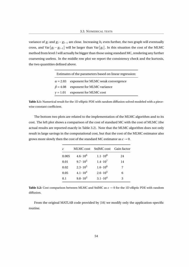
3.3. NUMERICAL TESTS
variance of gl and gl − gl−1 are close. Increasing hl even further, the two graph will eventually
cross, and Var[gl − gl−1
]will be larger than Var
[gl
]. In this situation the cost of the MLMC
method from level l will actually be bigger than those using standard MC, rendering any further
coarsening useless. In the middle row plot we report the consistency check and the kurtosis,
the two quantities defined above.
Estimates of the parameters based on linear regression:
α= 2.03 exponent for MLMC weak convergence
β= 4.08 exponent for MLMC variance
γ= 1.01 exponent for MLMC cost
Table 3.1: Numerical result for the 1D elliptic PDE with random diffusion solved modeled with a piece-
wise constant coefficient.
The bottom two plots are related to the implementation of the MLMC algorithm and to its
cost. The left plot shows a comparison of the cost of standard MC with the cost of MLMC (the
actual results are reported exactly in Table 3.2). Note that the MLMC algorithm does not only
result in large savings in the computational cost, but that the cost of the MLMC estimator also
grows more slowly then the cost of the standard MC estimator as ε→ 0.
ε MLMC cost StdMC cost Gain factor
0.005 4.6 ·106 1.1 ·108 24
0.01 9.7 ·105 1.4 ·107 14
0.02 2.3 ·105 1.6 ·106 7
0.05 4.1 ·104 2.6 ·105 6
0.1 9.8 ·103 3.1 ·104 3
Table 3.2: Cost comparison between MLMC and StdMC as ε→ 0 for the 1D elliptic PDE with random
diffusion.
From the original MATLAB code provided by [16] we modify only the application-specific
routine.
54
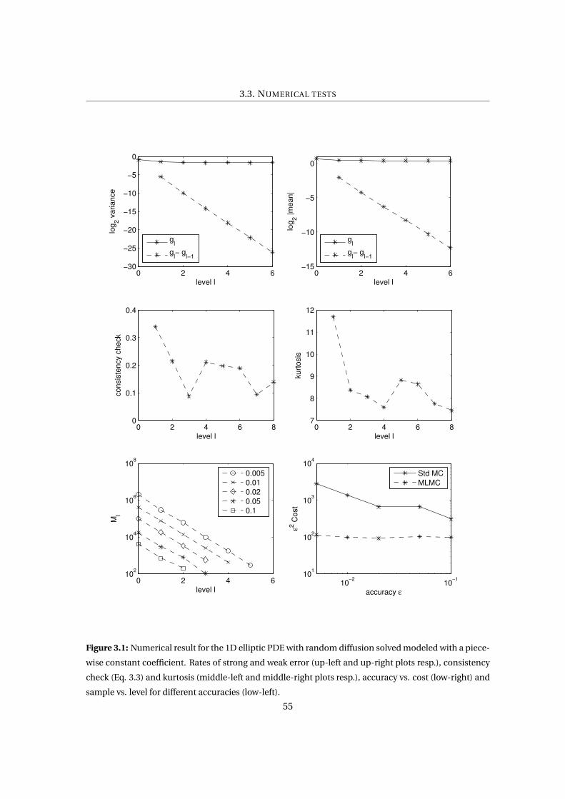
3.3. NUMERICAL TESTS
0 2 4 6 80
0.1
0.2
0.3
0.4
level l
consis
tency c
heck
0 2 4 6 87
8
9
10
11
12
level l
kurt
osis
0 2 4 610
2
104
106
108
level l
Ml
0.005
0.01
0.02
0.05
0.1
10−2
10−1
101
102
103
104
accuracy ε
ε2 C
ost
Std MC
MLMC
0 2 4 6−30
−25
−20
−15
−10
−5
0
level l
log
2 v
ariance
gl
gl− g
l−1
0 2 4 6−15
−10
−5
0
level llo
g2 |m
ean|
gl
gl− g
l−1
Figure 3.1: Numerical result for the 1D elliptic PDE with random diffusion solved modeled with a piece-
wise constant coefficient. Rates of strong and weak error (up-left and up-right plots resp.), consistency
check (Eq. 3.3) and kurtosis (middle-left and middle-right plots resp.), accuracy vs. cost (low-right) and
sample vs. level for different accuracies (low-left).
55
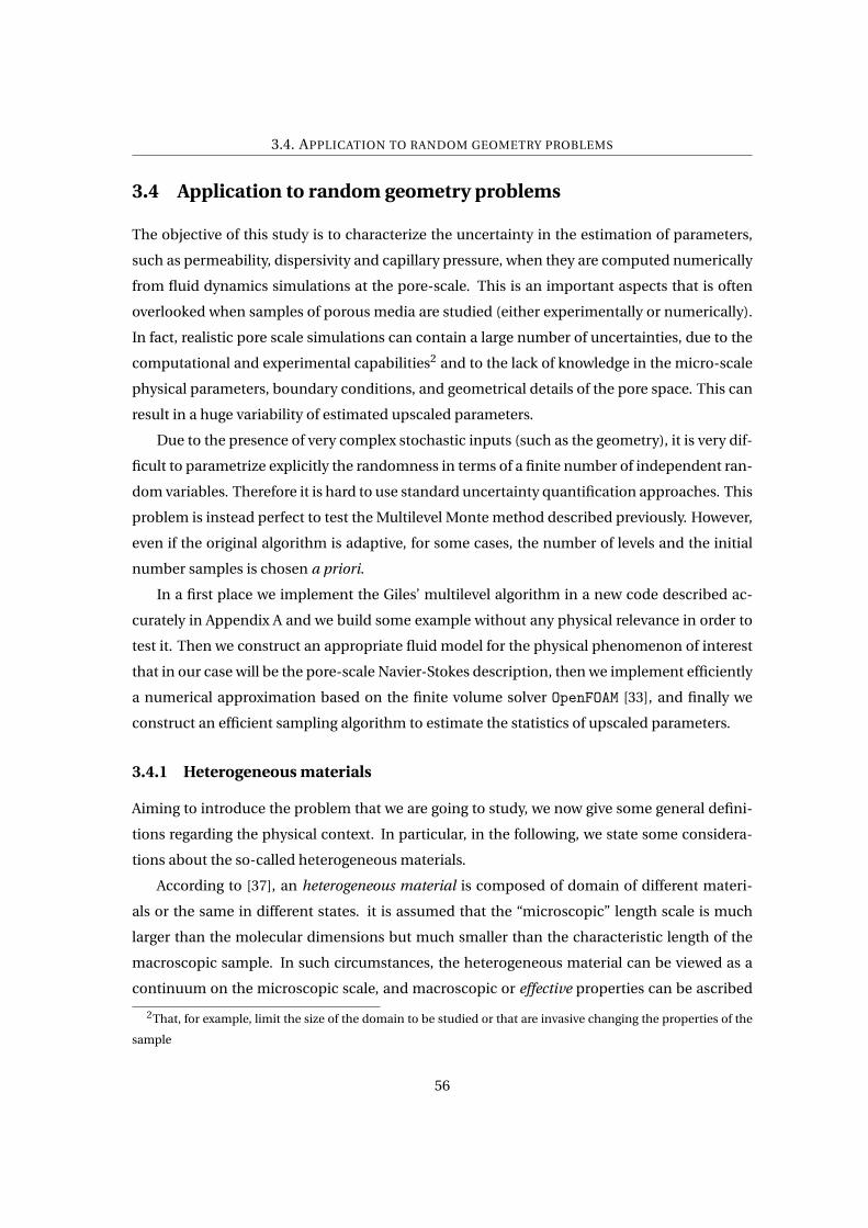
3.4. APPLICATION TO RANDOM GEOMETRY PROBLEMS
3.4 Application to random geometry problems
The objective of this study is to characterize the uncertainty in the estimation of parameters,
such as permeability, dispersivity and capillary pressure, when they are computed numerically
from fluid dynamics simulations at the pore-scale. This is an important aspects that is often
overlooked when samples of porous media are studied (either experimentally or numerically).
In fact, realistic pore scale simulations can contain a large number of uncertainties, due to the
computational and experimental capabilities2 and to the lack of knowledge in the micro-scale
physical parameters, boundary conditions, and geometrical details of the pore space. This can
result in a huge variability of estimated upscaled parameters.
Due to the presence of very complex stochastic inputs (such as the geometry), it is very dif-
ficult to parametrize explicitly the randomness in terms of a finite number of independent ran-
dom variables. Therefore it is hard to use standard uncertainty quantification approaches. This
problem is instead perfect to test the Multilevel Monte method described previously. However,
even if the original algorithm is adaptive, for some cases, the number of levels and the initial
number samples is chosen a priori.
In a first place we implement the Giles’ multilevel algorithm in a new code described ac-
curately in Appendix A and we build some example without any physical relevance in order to
test it. Then we construct an appropriate fluid model for the physical phenomenon of interest
that in our case will be the pore-scale Navier-Stokes description, then we implement efficiently
a numerical approximation based on the finite volume solver OpenFOAM [33], and finally we
construct an efficient sampling algorithm to estimate the statistics of upscaled parameters.
3.4.1 Heterogeneous materials
Aiming to introduce the problem that we are going to study, we now give some general defini-
tions regarding the physical context. In particular, in the following, we state some considera-
tions about the so-called heterogeneous materials.
According to [37], an heterogeneous material is composed of domain of different materi-
als or the same in different states. it is assumed that the “microscopic” length scale is much
larger than the molecular dimensions but much smaller than the characteristic length of the
macroscopic sample. In such circumstances, the heterogeneous material can be viewed as a
continuum on the microscopic scale, and macroscopic or effective properties can be ascribed
2That, for example, limit the size of the domain to be studied or that are invasive changing the properties of the
sample
56
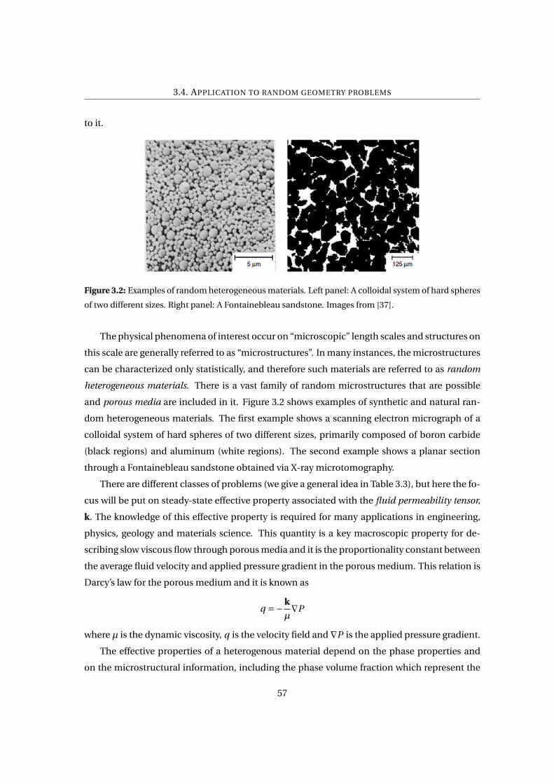
3.4. APPLICATION TO RANDOM GEOMETRY PROBLEMS
to it.
Figure 3.2: Examples of random heterogeneous materials. Left panel: A colloidal system of hard spheres
of two different sizes. Right panel: A Fontainebleau sandstone. Images from [37].
The physical phenomena of interest occur on “microscopic” length scales and structures on
this scale are generally referred to as “microstructures”. In many instances, the microstructures
can be characterized only statistically, and therefore such materials are referred to as random
heterogeneous materials. There is a vast family of random microstructures that are possible
and porous media are included in it. Figure 3.2 shows examples of synthetic and natural ran-
dom heterogeneous materials. The first example shows a scanning electron micrograph of a
colloidal system of hard spheres of two different sizes, primarily composed of boron carbide
(black regions) and aluminum (white regions). The second example shows a planar section
through a Fontainebleau sandstone obtained via X-ray microtomography.
There are different classes of problems (we give a general idea in Table 3.3), but here the fo-
cus will be put on steady-state effective property associated with the fluid permeability tensor,
k. The knowledge of this effective property is required for many applications in engineering,
physics, geology and materials science. This quantity is a key macroscopic property for de-
scribing slow viscous flow through porous media and it is the proportionality constant between
the average fluid velocity and applied pressure gradient in the porous medium. This relation is
Darcy’s law for the porous medium and it is known as
q =−k
µ∇P
where µ is the dynamic viscosity, q is the velocity field and ∇P is the applied pressure gradient.
The effective properties of a heterogenous material depend on the phase properties and
on the microstructural information, including the phase volume fraction which represent the
57
3.4. APPLICATION TO RANDOM GEOMETRY PROBLEMS
Class General effective Average (or applied) Average generalized
property (Ke ) generalized intensity (G) flux (F )
A Thermal conductivity Temperature gradient Heat flux
Diffusion coefficient Concentration gradient Mass flux
B Elastic moduli Strain field Stress field
C Survival time Species production rate Concentration field
D Fluid permeability Applied pressure gradient Velocity field
Sedimentation rate Force Mobility
Table 3.3: Different classes of steady-state effective media problems considered here. F ∝ KeG , where
Ke is the general effective property, G is the average (or applied) generalized gradient or intensity field,
and F is the average generalized flux field. Class A and B problems share many common features and
hence may be attacked using similar techniques. Class C and D problems are similarly related to one
another.
simplest level of information.
3.4.2 The geometry generation
After introducing the problem, we show how we can generate our stochastic realizations. The
first step requires to build a representative microscopic model of a porous media in order to
simulate fluid flow in these systems. There are many ways to obtain such model: one way
could be using real sample images, for example experimentally acquired by micro-computer
tomography techniques, another could be reconstructing realistically by means of suitable al-
gorithms. The latter is the one used by Icardi et al. in their work [10] and it simulate the sedi-
mentation of real three-dimensional grains, represented by convex polygonal surface meshes,
generating loose sand-like structures from given particle forms and grain size distribution. A
third way, the one we used in this work, could be placing point randomly in the domain until
the desired porosity is reached. We just remind that the definition of porosity is the volume of
grains over the total volume. This last method is less realistic and the model is far from a natural
porous media but it is more interesting, from a UQ point of view, to study the effect of a random
geometry. As already said, the problem is very complex and, in order to avoid the homogeniza-
tion phenomenon, we to consider a right number of grains. In one hand, if we have that too
many grains we will cause homogenization, therefore the multilevel algorithm would fail be-
cause the quantities, from one level to another will be uncorrelated. On the other hand, if we
58
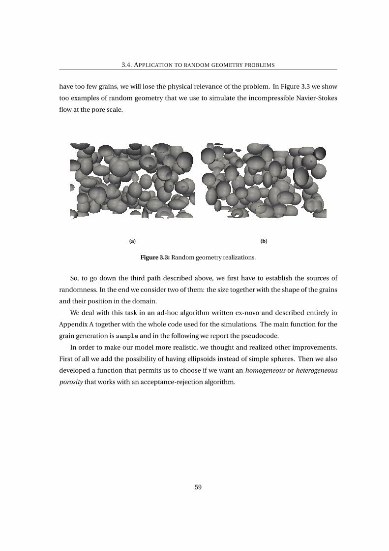
3.4. APPLICATION TO RANDOM GEOMETRY PROBLEMS
have too few grains, we will lose the physical relevance of the problem. In Figure 3.3 we show
too examples of random geometry that we use to simulate the incompressible Navier-Stokes
flow at the pore scale.
(a) (b)
Figure 3.3: Random geometry realizations.
So, to go down the third path described above, we first have to establish the sources of
randomness. In the end we consider two of them: the size together with the shape of the grains
and their position in the domain.
We deal with this task in an ad-hoc algorithm written ex-novo and described entirely in
Appendix A together with the whole code used for the simulations. The main function for the
grain generation is sample and in the following we report the pseudocode.
In order to make our model more realistic, we thought and realized other improvements.
First of all we add the possibility of having ellipsoids instead of simple spheres. Then we also
developed a function that permits us to choose if we want an homogeneous or heterogeneous
porosity that works with an acceptance-rejection algorithm.
59

3.4. APPLICATION TO RANDOM GEOMETRY PROBLEMS
Algorithm 4 sample()1: V0 → 2Lx ·2Ly ·2Lz (total domain volume)
2: V → 0 (grain volume)
3: for i = 1 → #grains do
4: p → (V0 −V )/V0 (check for porosity)
5: if desired porosity is reached then
6: break
7: end
8: if we do not want overlapping then
9: tries → 0
10: x ∼ Unif(−Lx ,Lx ), y ∼ Unif(−Ly ,Ly ), z ∼ Unif(−Lz ,Lz )
11: µ generated from a desired distribution (Uniform, Lognormal) or fixed
12: while max_tries is reached do
13: check for overlapping
14: tries → tries+1
15: if tries ≡ max_tries then
16: break
17: end
18: end
19: V =V + 43πµ
3
20: else
21: x ∼ Unif(−Lx ,Lx ), y ∼ Unif(−Ly ,Ly ), z ∼ Unif(−Lz ,Lz )
22: generate µ from desired distribution (Uniform, Lognormal)
23: V =V + VV0
43πµ
3 [“statistical” porosity calculation]
24: end
25: end
60
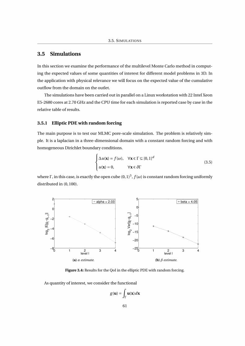
3.5. SIMULATIONS
3.5 Simulations
In this section we examine the performance of the multilevel Monte Carlo method in comput-
ing the expected values of some quantities of interest for different model problems in 3D. In
the application with physical relevance we will focus on the expected value of the cumulative
outflow from the domain on the outlet.
The simulations have been carried out in parallel on a Linux workstation with 22 Intel Xeon
E5-2680 cores at 2.70 GHz and the CPU time for each simulation is reported case by case in the
relative table of results.
3.5.1 Elliptic PDE with random forcing
The main purpose is to test our MLMC pore-scale simulation. The problem is relatively sim-
ple. It is a laplacian in a three-dimensional domain with a constant random forcing and with
homogeneous Dirichlet boundary conditions.∆u(x) = f (ω), ∀x ∈ Γ⊆ [0,1]d
u(x) = 0, ∀x ∈ ∂Γ(3.5)
where Γ, in this case, is exactly the open cube (0,1)3, f (ω) is constant random forcing uniformly
distributed in (0,100).
0 1 2 3 4−8
−6
−4
−2
0
2
level l
log
2 |E
[gl−
gl−
1]|
alpha = 2.03
(a) α estimate.
0 1 2 3 4−25
−20
−15
−10
−5
0
5
level l
log
2 V
ar[
g l−g
l−1]
beta = 4.05
(b) β estimate.
Figure 3.4: Results for the QoI in the elliptic PDE with random forcing.
As quantity of interest, we consider the functional
g (u) =∫Γ
u(x)dx
61
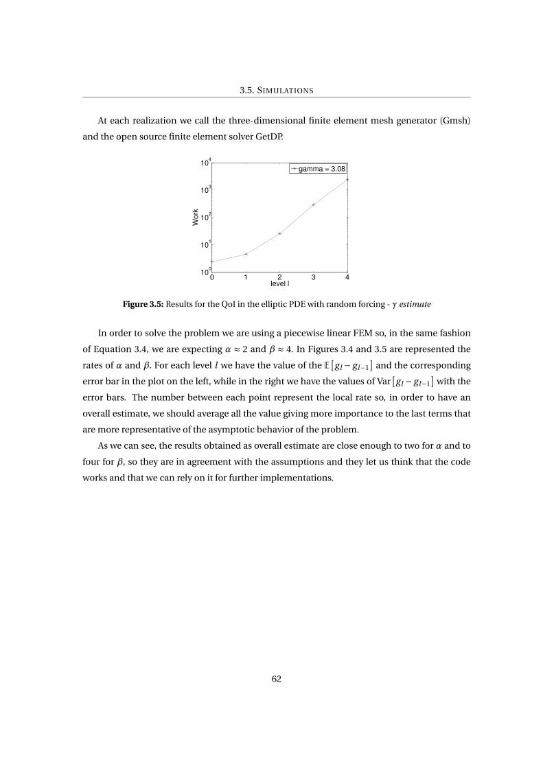
3.5. SIMULATIONS
At each realization we call the three-dimensional finite element mesh generator (Gmsh)
and the open source finite element solver GetDP.
0 1 2 3 410
0
101
102
103
104
level l
Wo
rk
gamma = 3.08
Figure 3.5: Results for the QoI in the elliptic PDE with random forcing - γ estimate
In order to solve the problem we are using a piecewise linear FEM so, in the same fashion
of Equation 3.4, we are expecting α ≈ 2 and β ≈ 4. In Figures 3.4 and 3.5 are represented the
rates of α and β. For each level l we have the value of the E[gl − gl−1
]and the corresponding
error bar in the plot on the left, while in the right we have the values of Var[gl − gl−1
]with the
error bars. The number between each point represent the local rate so, in order to have an
overall estimate, we should average all the value giving more importance to the last terms that
are more representative of the asymptotic behavior of the problem.
As we can see, the results obtained as overall estimate are close enough to two for α and to
four for β, so they are in agreement with the assumptions and they let us think that the code
works and that we can rely on it for further implementations.
62
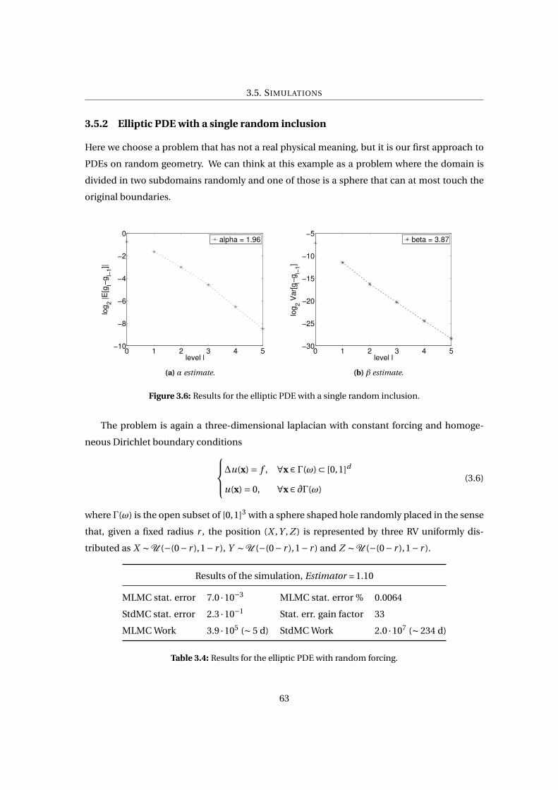
3.5. SIMULATIONS
3.5.2 Elliptic PDE with a single random inclusion
Here we choose a problem that has not a real physical meaning, but it is our first approach to
PDEs on random geometry. We can think at this example as a problem where the domain is
divided in two subdomains randomly and one of those is a sphere that can at most touch the
original boundaries.
0 1 2 3 4 5−10
−8
−6
−4
−2
0
level l
log
2 |E
[gl−
gl−
1]|
alpha = 1.96
(a) α estimate.
0 1 2 3 4 5−30
−25
−20
−15
−10
−5
level l
log
2 V
ar[
g l−g
l−1]
beta = 3.87
(b) β estimate.
Figure 3.6: Results for the elliptic PDE with a single random inclusion.
The problem is again a three-dimensional laplacian with constant forcing and homoge-
neous Dirichlet boundary conditions∆u(x) = f , ∀x ∈ Γ(ω) ⊂ [0,1]d
u(x) = 0, ∀x ∈ ∂Γ(ω)(3.6)
where Γ(ω) is the open subset of [0,1]3 with a sphere shaped hole randomly placed in the sense
that, given a fixed radius r , the position (X ,Y , Z ) is represented by three RV uniformly dis-
tributed as X ∼U (−(0− r ),1− r ), Y ∼U (−(0− r ),1− r ) and Z ∼U (−(0− r ),1− r ).
Results of the simulation, Estimator = 1.10
MLMC stat. error 7.0 ·10−3 MLMC stat. error % 0.0064
StdMC stat. error 2.3 ·10−1 Stat. err. gain factor 33
MLMC Work 3.9 ·105 (∼ 5 d) StdMC Work 2.0 ·107 (∼ 234 d)
Table 3.4: Results for the elliptic PDE with random forcing.
63
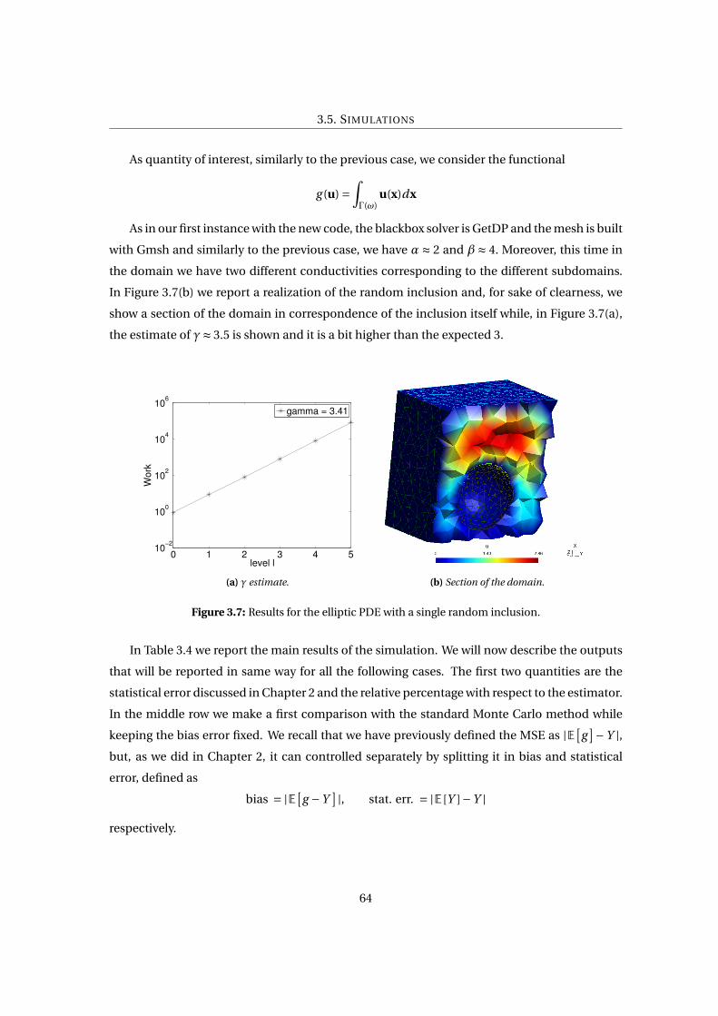
3.5. SIMULATIONS
As quantity of interest, similarly to the previous case, we consider the functional
g (u) =∫Γ(ω)
u(x)dx
As in our first instance with the new code, the blackbox solver is GetDP and the mesh is built
with Gmsh and similarly to the previous case, we have α ≈ 2 and β ≈ 4. Moreover, this time in
the domain we have two different conductivities corresponding to the different subdomains.
In Figure 3.7(b) we report a realization of the random inclusion and, for sake of clearness, we
show a section of the domain in correspondence of the inclusion itself while, in Figure 3.7(a),
the estimate of γ≈ 3.5 is shown and it is a bit higher than the expected 3.
0 1 2 3 4 510
−2
100
102
104
106
level l
Wo
rk
gamma = 3.41
(a) γ estimate. (b) Section of the domain.
Figure 3.7: Results for the elliptic PDE with a single random inclusion.
In Table 3.4 we report the main results of the simulation. We will now describe the outputs
that will be reported in same way for all the following cases. The first two quantities are the
statistical error discussed in Chapter 2 and the relative percentage with respect to the estimator.
In the middle row we make a first comparison with the standard Monte Carlo method while
keeping the bias error fixed. We recall that we have previously defined the MSE as |E[g]−Y |,
but, as we did in Chapter 2, it can controlled separately by splitting it in bias and statistical
error, defined as
bias = |E[g −Y
] |, stat. err. = |E [Y ]−Y |
respectively.
64
3.5. SIMULATIONS
The statistical error of a single level is computed as
StdMC stat. err = c0
√Var
[gL
]ML
(3.7)
and it represents, the statistical error that would be achieved with only the last single level. In
order to give an idea of the improvement we also report the gain factor that is simply the ratio
between the statistical of the single level and the original statistical error. Finally the last two
quantities are the MLMC work and the standard Monte Carlo one. The previous is computed
directly as the sum of the CPU time in each level
L∑l=0
Ml ·Wl
while the latter is an estimate computed as
MMC ·WL
where the number of Monte Carlo samples is calculated using Equation 3.7, replacing the single
level statistical error with the standard one and then solving for ML . In other words, these last
two quantities represent a comparison of the work for the same level of error.
As we can see from the Table 3.4, even for this simple the standard Monte Carlo method is
clearly outperformed. In Table 3.7, instead, we make a statement on the theoretical complexity.
65
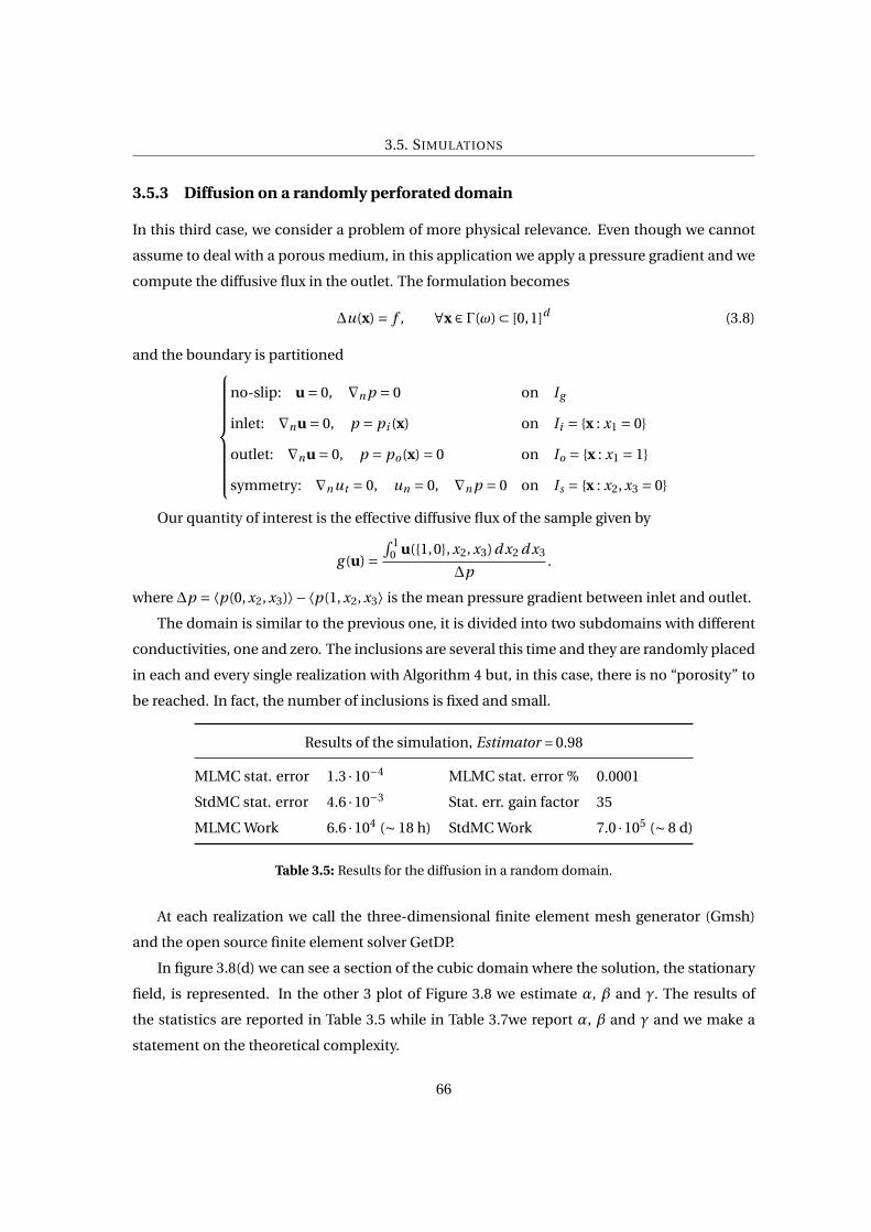
3.5. SIMULATIONS
3.5.3 Diffusion on a randomly perforated domain
In this third case, we consider a problem of more physical relevance. Even though we cannot
assume to deal with a porous medium, in this application we apply a pressure gradient and we
compute the diffusive flux in the outlet. The formulation becomes
∆u(x) = f , ∀x ∈ Γ(ω) ⊂ [0,1]d (3.8)
and the boundary is partitioned
no-slip: u = 0, ∇n p = 0 on Ig
inlet: ∇nu = 0, p = pi (x) on Ii = {x : x1 = 0}
outlet: ∇nu = 0, p = po(x) = 0 on Io = {x : x1 = 1}
symmetry: ∇nut = 0, un = 0, ∇n p = 0 on Is = {x : x2, x3 = 0}
Our quantity of interest is the effective diffusive flux of the sample given by
g (u) =∫ 1
0 u({1,0}, x2, x3)d x2 d x3
∆p.
where ∆p = ⟨p(0, x2, x3)⟩−⟨p(1, x2, x3⟩ is the mean pressure gradient between inlet and outlet.
The domain is similar to the previous one, it is divided into two subdomains with different
conductivities, one and zero. The inclusions are several this time and they are randomly placed
in each and every single realization with Algorithm 4 but, in this case, there is no “porosity” to
be reached. In fact, the number of inclusions is fixed and small.
Results of the simulation, Estimator = 0.98
MLMC stat. error 1.3 ·10−4 MLMC stat. error % 0.0001
StdMC stat. error 4.6 ·10−3 Stat. err. gain factor 35
MLMC Work 6.6 ·104 (∼ 18 h) StdMC Work 7.0 ·105 (∼ 8 d)
Table 3.5: Results for the diffusion in a random domain.
At each realization we call the three-dimensional finite element mesh generator (Gmsh)
and the open source finite element solver GetDP.
In figure 3.8(d) we can see a section of the cubic domain where the solution, the stationary
field, is represented. In the other 3 plot of Figure 3.8 we estimate α, β and γ. The results of
the statistics are reported in Table 3.5 while in Table 3.7we report α, β and γ and we make a
statement on the theoretical complexity.
66
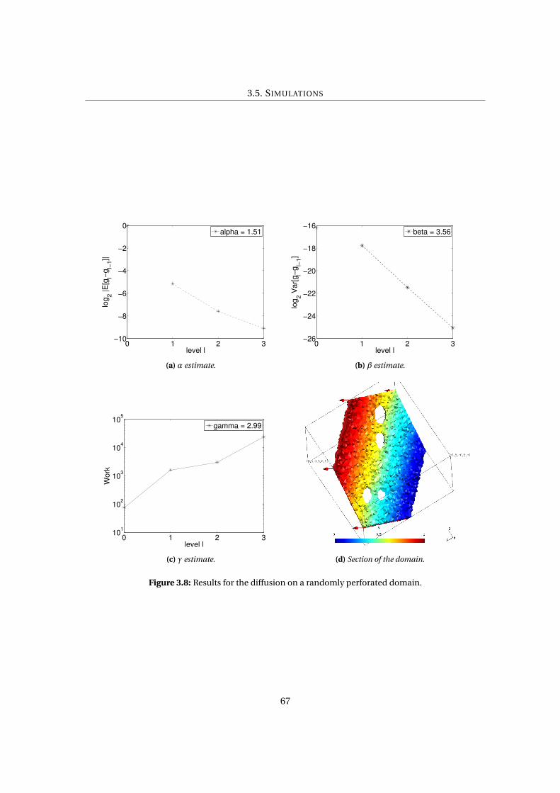
3.5. SIMULATIONS
0 1 2 3−10
−8
−6
−4
−2
0
level l
log
2 |E
[gl−
gl−
1]|
alpha = 1.51
(a) α estimate.
0 1 2 3−26
−24
−22
−20
−18
−16
level l
log
2 V
ar[
g l−g
l−1]
beta = 3.56
(b) β estimate.
0 1 2 310
1
102
103
104
105
level l
Wo
rk
gamma = 2.99
(c) γ estimate. (d) Section of the domain.
Figure 3.8: Results for the diffusion on a randomly perforated domain.
67
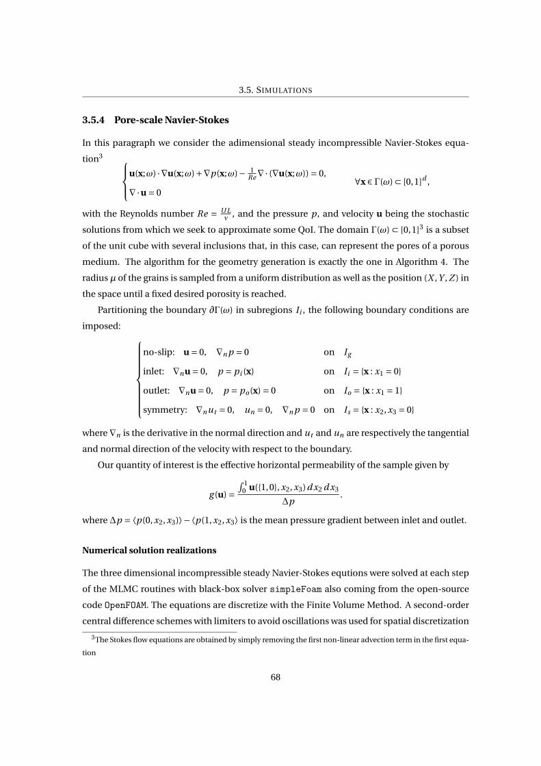
3.5. SIMULATIONS
3.5.4 Pore-scale Navier-Stokes
In this paragraph we consider the adimensional steady incompressible Navier-Stokes equa-
tion3 u(x;ω) ·∇u(x;ω)+∇p(x;ω)− 1Re ∇· (∇u(x;ω)) = 0,
∇·u = 0∀x ∈ Γ(ω) ⊂ [0,1]d ,
with the Reynolds number Re = U Lν , and the pressure p, and velocity u being the stochastic
solutions from which we seek to approximate some QoI. The domain Γ(ω) ⊂ [0,1]3 is a subset
of the unit cube with several inclusions that, in this case, can represent the pores of a porous
medium. The algorithm for the geometry generation is exactly the one in Algorithm 4. The
radius µ of the grains is sampled from a uniform distribution as well as the position (X ,Y , Z ) in
the space until a fixed desired porosity is reached.
Partitioning the boundary ∂Γ(ω) in subregions Ii , the following boundary conditions are
imposed:
no-slip: u = 0, ∇n p = 0 on Ig
inlet: ∇nu = 0, p = pi (x) on Ii = {x : x1 = 0}
outlet: ∇nu = 0, p = po(x) = 0 on Io = {x : x1 = 1}
symmetry: ∇nut = 0, un = 0, ∇n p = 0 on Is = {x : x2, x3 = 0}
where ∇n is the derivative in the normal direction and ut and un are respectively the tangential
and normal direction of the velocity with respect to the boundary.
Our quantity of interest is the effective horizontal permeability of the sample given by
g (u) =∫ 1
0 u({1,0}, x2, x3)d x2 d x3
∆p.
where ∆p = ⟨p(0, x2, x3)⟩−⟨p(1, x2, x3⟩ is the mean pressure gradient between inlet and outlet.
Numerical solution realizations
The three dimensional incompressible steady Navier-Stokes equtions were solved at each step
of the MLMC routines with black-box solver simpleFoam also coming from the open-source
code OpenFOAM. The equations are discretize with the Finite Volume Method. A second-order
central difference schemes with limiters to avoid oscillations was used for spatial discretization
3The Stokes flow equations are obtained by simply removing the first non-linear advection term in the first equa-
tion
68
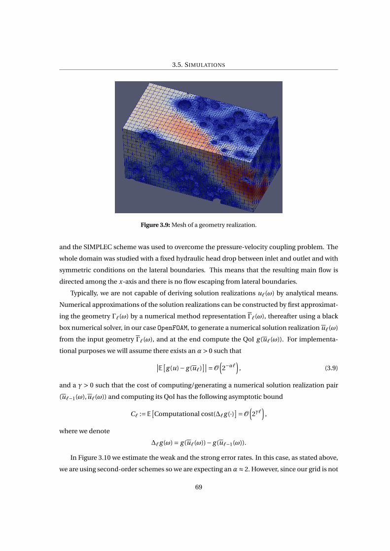
3.5. SIMULATIONS
Figure 3.9: Mesh of a geometry realization.
and the SIMPLEC scheme was used to overcome the pressure-velocity coupling problem. The
whole domain was studied with a fixed hydraulic head drop between inlet and outlet and with
symmetric conditions on the lateral boundaries. This means that the resulting main flow is
directed among the x-axis and there is no flow escaping from lateral boundaries.
Typically, we are not capable of deriving solution realizations u`(ω) by analytical means.
Numerical approximations of the solution realizations can be constructed by first approximat-
ing the geometry Γ`(ω) by a numerical method representation Γ`(ω), thereafter using a black
box numerical solver, in our case OpenFOAM, to generate a numerical solution realization u`(ω)
from the input geometry Γ`(ω), and at the end compute the QoI g (u`(ω)). For implementa-
tional purposes we will assume there exists an α> 0 such that∣∣E[g (u)− g (u`)
]∣∣=O(2−α`
), (3.9)
and a γ > 0 such that the cost of computing/generating a numerical solution realization pair
(u`−1(ω),u`(ω)) and computing its QoI has the following asymptotic bound
C` := E[Computational cost(∆`g (·)]=O
(2γ`
),
where we denote
∆`g (ω) = g (u`(ω))− g (u`−1(ω)).
In Figure 3.10 we estimate the weak and the strong error rates. In this case, as stated above,
we are using second-order schemes so we are expecting anα≈ 2. However, since our grid is not
69
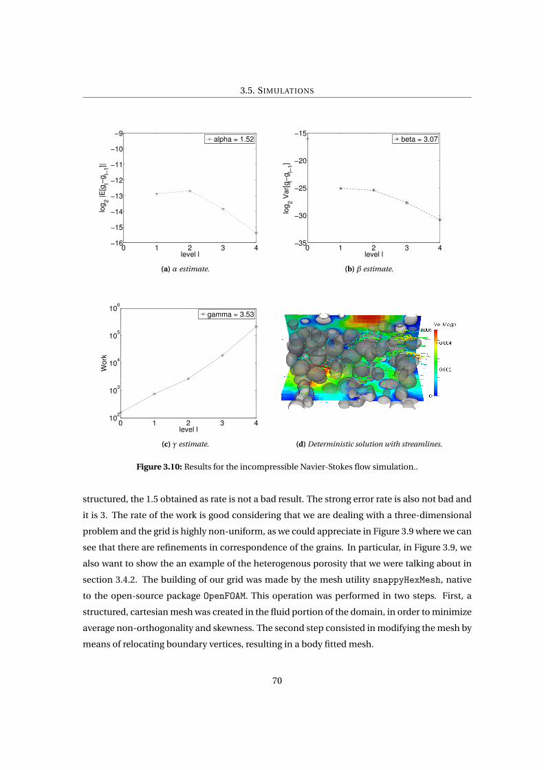
3.5. SIMULATIONS
0 1 2 3 4−16
−15
−14
−13
−12
−11
−10
−9
level l
log
2 |E
[gl−
gl−
1]|
alpha = 1.52
(a) α estimate.
0 1 2 3 4−35
−30
−25
−20
−15
level l
log
2 V
ar[
g l−g
l−1]
beta = 3.07
(b) β estimate.
0 1 2 3 410
2
103
104
105
106
level l
Wo
rk
gamma = 3.53
(c) γ estimate. (d) Deterministic solution with streamlines.
Figure 3.10: Results for the incompressible Navier-Stokes flow simulation..
structured, the 1.5 obtained as rate is not a bad result. The strong error rate is also not bad and
it is 3. The rate of the work is good considering that we are dealing with a three-dimensional
problem and the grid is highly non-uniform, as we could appreciate in Figure 3.9 where we can
see that there are refinements in correspondence of the grains. In particular, in Figure 3.9, we
also want to show the an example of the heterogenous porosity that we were talking about in
section 3.4.2. The building of our grid was made by the mesh utility snappyHexMesh, native
to the open-source package OpenFOAM. This operation was performed in two steps. First, a
structured, cartesian mesh was created in the fluid portion of the domain, in order to minimize
average non-orthogonality and skewness. The second step consisted in modifying the mesh by
means of relocating boundary vertices, resulting in a body fitted mesh.
70
3.5. SIMULATIONS
Results of the simulation, Estimator = 2.1753 ·10−3
MLMC stat. error 1.3 ·10−4 MLMC stat. err. % 0.0617
StdMC stat. error 4.9 ·10−2 Stat. err. gain factor 362
MLMC Work 4.6 ·105 (∼ 5 d) StdMC Work 1.7 ·107 (∼ 191 d)
Table 3.6: Results for the incompressible Navier-Stokes flow simulation.
In Table 3.6 we report the results of the simulation and, similarly to the other cases, the
advantages of the MLMC method is clear. In this case we can see how the standard Monte
Carlo is not only outperformed, but also it would be impossible to realize in a reasonable time.
In Table 3.7we report α, β and γ and we make a statement on the theoretical complexity.
71
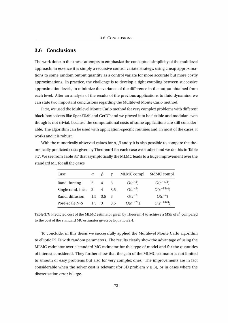
3.6. CONCLUSIONS
3.6 Conclusions
The work done in this thesis attempts to emphasize the conceptual simplicity of the multilevel
approach; in essence it is simply a recursive control variate strategy, using cheap approxima-
tions to some random output quantity as a control variate for more accurate but more costly
approximations. In practice, the challenge is to develop a tight coupling between successive
approximation levels, to minimize the variance of the difference in the output obtained from
each level. After an analysis of the results of the previous applications to fluid dynamics, we
can state two important conclusions regarding the Multilevel Monte Carlo method.
First, we used the Multilevel Monte Carlo method for very complex problems with different
black-box solvers like OpenFOAM and GetDP and we proved it to be flexible and modular, even
though is not trivial, because the computational costs of some applications are still consider-
able. The algorithm can be used with application-specific routines and, in most of the cases, it
works and it is robust.
With the numerically observed values for α, β and γ it is also possible to compare the the-
oretically predicted costs given by Theorem 4 for each case we studied and we do this in Table
3.7. We see from Table 3.7 that asymptotically the MLMC leads to a huge improvement over the
standard MC for all the cases.
Case α β γ MLMC compl. StdMC compl.
Rand. forcing 2 4 3 O(ε−2) O(ε−7/2)
Single rand. incl. 2 4 3.5 O(ε−2) O(ε−15/4)
Rand. diffusion 1.5 3.5 3 O(ε−2) O(ε−4)
Pore-scale N-S 1.5 3 3.5 O(ε−7/3) O(ε−13/3)
Table 3.7: Predicted cost of the MLMC estimator given by Theorem 4 to achieve a MSE of ε2 compared
to the cost of the standard MC estimator given by Equation 2.4.
To conclude, in this thesis we successfully applied the Multilevel Monte Carlo algorithm
to elliptic PDEs with random parameters. The results clearly show the advantage of using the
MLMC estimator over a standard MC estimator for this type of model and for the quantities
of interest considered. They further show that the gain of the MLMC estimator is not limited
to smooth or easy problems but also for very complex ones. The improvements are in fact
considerable when the solver cost is relevant (for 3D problem γ ≥ 3), or in cases where the
discretization error is large.
72
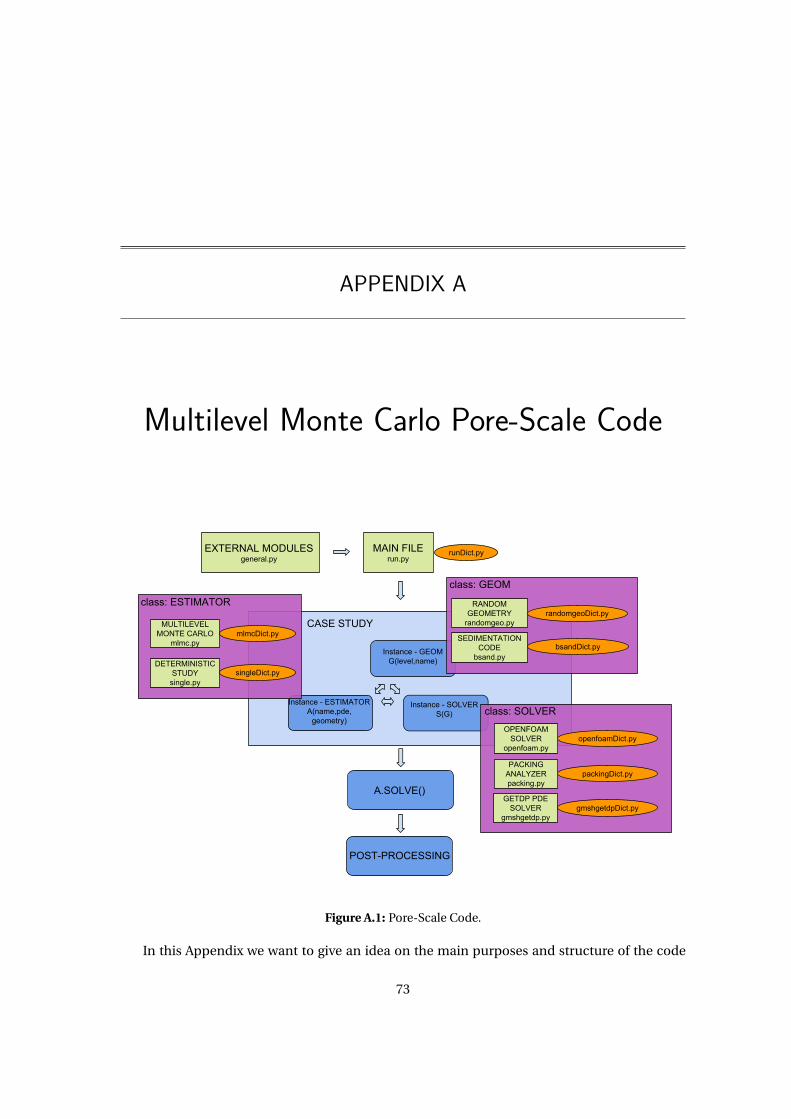
APPENDIX A
Multilevel Monte Carlo Pore-Scale Code
MAIN FILErun.py
runDict.pyEXTERNAL MODULESgeneral.py
POST-PROCESSING
A.SOLVE()
CASE STUDY
Instance - SOLVERS(G)
Instance - GEOMG(level,name)
Instance - ESTIMATORA(name,pde,
geometry)
MULTILEVEL MONTE CARLO
mlmc.py
DETERMINISTIC STUDY
single.py
mlmcDict.py
singleDict.py
class: ESTIMATOR
openfoamDict.py
gmshgetdpDict.py
packingDict.py
OPENFOAM SOLVER
openfoam.py
PACKING ANALYZERpacking.py
GETDP PDE SOLVER
gmshgetdp.py
class: SOLVER
randomgeoDict.py
bsandDict.py
RANDOM GEOMETRY
randomgeo.py
SEDIMENTATION CODE
bsand.py
class: GEOM
Figure A.1: Pore-Scale Code.
In this Appendix we want to give an idea on the main purposes and structure of the code
73
A.1. MAIN PURPOSE
we used for the MLMC simulations presented in this thesis. In Figure A.1 we show a schematic
representation of its main features that we will explain in details below. The code [27] has been
structured as a wrapper, developed in Python, containing calls to external sub-modules. An
object-oriented programming paradigm has been used, by creating abstract classes of different
types whose multiple instances are then created.
A.1 Main purpose
After understanding the potentialities of multilevel Monte Carlo and after a deep study of Giles’
algorithm we extended the code in order to apply the method to more complex problems such
as the ones described in Chapter 3. To do this, we need to combine existing solvers of different
types and generate complex pre- and post- processing routines. The code has been structured
as a “general-purpose” MLMC estimator for complex computational problems therefore with a
high level of abstraction and flexibility.
The basis of the code was initially thought to solve a finite number of deterministic prob-
lems like the ones in [26], where the fluid flow and the solute transport through porous media
are described. Since we had in mind something that could work in a wider spectrum of prob-
lems and with different approaches, we extended it also for statistical estimation of random
PDE, keeping the physical complexity of the problems.We ended up with a code that can deal
with deterministic and statistical problems that can solve different PDE model equations. This
is achieved by calling external solvers such as OpenFOAM , GetDP and Fenics in order to solve
problems like Steady State Navier-Stokes, two-phases compressible flows, two-phases incom-
pressible flows, Darcy, Laplacian, etc.
A.2 Structure
The main script of the whole program is run.py where all the external modules are imported,
the main settings of the estimation are loaded and the main object, containing (called es-
timator) is created and solved. All the settings are imported from dictionary files, such as
runDict.py. Every part of the program, in fact, is associated with a dictionary where the pa-
rameters are stored and can be easily configured by the user, as we can clearly see in Figure
A.1. As we can also see from Figure A.1, there are three classes that characterize the three main
elements of each problem. Each of these elements can be loaded by different files, according
to the problem we want to solve
74
A.2. STRUCTURE
From the first one, the Estimator class, we can choose the approach of problem. In fact, if
we want to estimate a quantity of interest with the multilevel Monte Carlo method we create
an instance with mlmc.py, on the other hand, if we want to find a deterministic solution or
a fixed parametric study of a given problem we create an instance with single.py. In the
former the Giles’ multilevel algorithm and other similar algorithms are implemented. They
can be adaptive, like the original one, or we can set a priori some parameters like the initial
number of sample and number of levels. These parameters, together with the confidence (c0),
the tolerance (ε or TOL) and the splitting between the bias and the statistical error, can be set
in mlmcDict.py WIth the latter instead, a single deterministic simulations can be run.
After the estimator has been created and set up, it is solved by running the selected algo-
rithm, implemented in the class itself. To do this usually a second class is used, called Geom
class that store all the information of the geometry. For each realization an instance of the
Geom class is created. Two kind of geometries can be created. With randomgeo.py the geom-
etry is constructed, as we have already well seen in Chapter 3, as a realization of two random
variables, one for the position of the grains (if we deal with a porous medium) or the position
of the inclusion (if we do not deal with a physically relevant problem), and one for the char-
acteristic dimension of the grain/inclusion, i.e. the radius. With bsand.py instead, a realistic
porous medium geometry can be created. In this latter case, is simulated the sedimentation of
the real three-dimensional grains, represented by convex polygonal surface meshes, generat-
ing loose sand-like structures from given particle forms and grain size distributions. The actual
grain shape and grain size distributions are obtained respectively by two-dimensional scan-
ning electron microscopy (SEM) scans and static-light scattering measurements carried out on
standard sand samples.
A third and last is Solver class. Has to do with the all the settings and routines specific for
each solver. A geometry is passed to construct a solver object on top of it. The solver is de-
fined in three files, openfoam.py, gmshgetdp.py and packing.py, in order to define which
code to use to solve our problem. The first has the obvious connection with the open-source
code OpenFOAM1. In this case, each time a sample is realized and the geometry is built, it creates
the mesh with the utility snappyHexMesh and it calls the right solver suitable for the problem
we are trying to solve (for our problems simpleFoam, the steady-state solver for incompress-
ible and turbulent flows). The second solver, instead, is linked to Gmsh2, a three-dimensional
1website - http://www.openfoam.com2website - http://geuz.org/gmsh/
75
A.3. FINAL STATEMENTS
finite element mesh generator, and GetDP3 (“General environment for the treatment of Dis-
crete Problems”), an open-source scientific software environment for the numerical solution
of integro-differential equations, open to the coupling of physical problems (electromagnetic,
thermal, etc.) as well as of numerical methods (finite element method, integral methods, etc.)
which can deal with such problems of various dimensions (1D, 2D or 3D) and time states (static,
transient or harmonic). The last but not least, packing.py is not aPDE solver, but it is though
to run statistical analysis’ on the geometry realizations once they are generated.
After each geometry and solver instances are created, the problem is solved, the quantities
of interest are stored in the estimator object and adaptively used for estimation. When the algo-
rithm stops results are plotted and a post-processing analysis can be conducted. It is important
to highlight that, being the Monte Carlo samples independent, the code can be parallelized at
two levels: the level of the MLMC estimator and the level of the single solver. Both of these
approaches have been used and combined.
A.3 Final statements
During the whole process of the thesis development we run many test cases to test and debug
the code and, in the end, we can say to have proved its effectiveness in important applications.
However, due to the complexity of the problems at hand, there is still space to many fur-
ther improvements related to performance, parallelization, analysis of convergence and non-
asymptotic behaviors. Also the extension to different problems and the linking to other external
software would be something extremely interesting for future works.
3website - http://www.geuz.org/getdp/
76

Bibliography
[1] S. Asmussen, P. W. Glynn Stochastic Simulation, Algorithms and Analysis, Springer, 2007.
[2] I. Babuška, F. Nobile, R. Tempone A stochastic collocation method for elliptic partial differ-
ential equations with random input data, SIAM Review 52(2), 2010.
[3] I. Babuška, R. Tempone, G. Zouraris Galerkin finite element approximations of stochastic
elliptic partial differential equations, SIAM Journal on Numerical Analysis 42(2), 800-825,
2004.
[4] J. Baldeaux, M. Gnewuch, ‘Optimal randomized multilevel algorithms for infinite-
dimensional integration on function spaces with ANOVA-type decomposition, SIAM Journal
of Numerical Analysis 52(3), 1128–1155, 2014.
[5] A. Barth, C. Schwab, N. Zollinger Multilevel Monte Carlo finite element method for elliptic
PDEs with stochastic coefficients Numer. Math. Online First, 2011.
[6] J. Bear Dynamics of fluids in porous media, Dover Publications, 1988.
[7] C. Canuto Notes on Partial Differential Equation, 2009.
[8] C. Canuto, S. Berrone Notes on Numerical Methods for Partial Differential Equation, 2011.
[9] K. A. Cliffe, M. B. Giles, R. Scheichl, A. L. Teckentrup Multilevel Monte Carlo methods and
application to elliptic PDEs with random coefficients, Springer-Verlag 2011.
[10] N. Collier, A. Haji-Ali, F. Nobile, E. von Schwerin, R. Tempone, A Continuation Multilevel
Monte Carlo algorithm, 2014.
77
BIBLIOGRAPHY
[11] J. Dick, M. Gnewuch Infinite-dimensional integration in weighted Hilbert spaces: anchored
decompositions, optimal deterministic algorithms, and higher order convergence, Founda-
tion of Computational Mathematics 184, 111–145, 2014a
[12] J. Dick, M. Gnewuch Optimal randomized changing dimension algorithms for infinite-
dimensional integration on function spaces with ANOVA-type decomposition, Journal of Ap-
proximation Theory 184, 111–145, 2014b
[13] J. Dick, F. Y. Kuo, I. H. Sloan High-dimensional integration: The quasi-Monte Carlo way,
Acta Numerica / Volume 22 / May 2013, pp 133-288.
[14] J. H. Ferziger, M. Peric Computational Methods for Fluid Dynamics, Springer-Verlag, 2002
[15] M. B. Giles, Multilevel Monte Carlo path simulation, Oxford, UK.
[16] M. B. Giles, Multilevel Monte Carlo methods, Oxford (2015), UK.
[17] M. B. Giles, B. Waterhouse Multilevel quasi-Monte Carlo path simulation, Advanced Fi-
nancial Modelling, Radon Series on Computational and Applied Mathematics, 165-181,
2009.
[18] P. Glasserman Monte Carlo Methods in FInancial Engineering, Springer, 2003.
[19] M. Gunzburger, C. Webster, G. Zhang Stochastic finite element methods for partial differ-
ential equations with random input data, Acta Numerica 23, 2014.
[20] A. Haji-Ali, F. Nobile, E. von Schwerin, R. Tempone, Optimization of mesh hierarchies in
Multilevel Monte Carlo samplers, 2014.
[21] S. Heinrich, Monte Carlo complexity of global solution of integral equations, Journal of
Complexity 14(2), 151-175, 1998.
[22] S. Heinrich, E. Sindambiwe Monte Carlo complexity of parametric integration, Journal of
Complexity 15(3), 317-341, 1999.
[23] A. Kebaier Statistical Romberg extrapolation: a new variance reduction method and appli-
cations to options pricing, Annals of Applied Probability 14(4), 2681-2705, 2005.
[24] F. Y. Kuo, C. Schwab, I. H. Sloan ‘Multi-level quasi-Monte Carlo finite element methods for a
class of elliptic partial differential equations with random coefficients, ArXiv preprint:, 2012.
78
BIBLIOGRAPHY
[25] G. Iaccarino, T. Magin, Short Course on Uncertainty Quantification, Stanford CA, USA.
[26] M. Icardi, G. Boccardo, T. Tosco, D. L. Marchisio, R. Sethi, Pore-scale simulation of fluid
flow and solute dispersion in three-dimensional porous media, 2014.
[27] M. Icardi, R. Tempone, Multilevel Monte Carlo Applications to Geometrical and Differential
Problems on Random Geometry, (in preparation).
[28] O. P. Le Maître, O. M. Knio, Spectral Methods for Uncertainty Quantification, Springer
[29] C. Lemieux, Monte Carlo and Quasi-Monte Carlo Sampling, Springer, 2009.
[30] G. Migliorati, F. Nobile, E. von Schwerin, R. Tempone, Analysis of the discrete L2 projection
on polynomial spaces with random evaluation, 2011.
[31] B. Niu, F. Hickernell, T. Müller-Gronbach, K. Ritter Deterministic multi-level algorithms for
infinite-dimensional integration on RN , Journal of Complexity 27(3-4), 331-351, 2010.
[32] F. Nobile, R. Tempone, Mathematical and Algorithmic Aspects of Uncertainty Quantication
Summer School at University of Texas, slides, 2014.
[33] OpenCFD The Open Source CFD Toolbox, User Guide, OpenCFD (ESI), 2013.
[34] M. Putko, A. Taylor, P. Newmann, L. Green Approach for input uncertainty propagation
and robust design in CFD using sensitivity derivatives, Journal of Fluids Engineering 124(1),
60-69, 2002.
[35] D. S. Sivia, Data Analysis, a Bayesian Tutorial, Oxford University Press, 2006.
[36] A. Stuart, Uncertainty Quantification in Bayesian Inversion, 2010.
[37] S. Torquato, Random Heterogeneous Materials: Microstructure and Macroscopic Proper-
ties, Springer-Verlag, 2002.
[38] D. Xiu, G. Karniadakis The Wiener–Askey polynomial chaos for stochastic differential equa-
tions, SIAM Journal on Scientific Computing, 2002.
79