Multiobjective Design and Innovization of Robust

University of VermontScholarWorks @ UVM

Graduate College Dissertations and Theses Dissertations and Theses

2013

Multiobjective Design and Innovization of RobustStormwater Management PlansKarim ChichaklyUniversity of Vermont

Follow this and additional works at: https://scholarworks.uvm.edu/graddis

Part of the Computer Sciences Commons

This Dissertation is brought to you for free and open access by the Dissertations and Theses at ScholarWorks @ UVM. It has been accepted forinclusion in Graduate College Dissertations and Theses by an authorized administrator of ScholarWorks @ UVM. For more information, please [email protected].

Recommended CitationChichakly, Karim, "Multiobjective Design and Innovization of Robust Stormwater Management Plans" (2013). Graduate CollegeDissertations and Theses. 2.https://scholarworks.uvm.edu/graddis/2

https://scholarworks.uvm.edu?utm_source=scholarworks.uvm.edu%2Fgraddis%2F2&utm_medium=PDF&utm_campaign=PDFCoverPages

https://scholarworks.uvm.edu/graddis?utm_source=scholarworks.uvm.edu%2Fgraddis%2F2&utm_medium=PDF&utm_campaign=PDFCoverPages

https://scholarworks.uvm.edu/etds?utm_source=scholarworks.uvm.edu%2Fgraddis%2F2&utm_medium=PDF&utm_campaign=PDFCoverPages

https://scholarworks.uvm.edu/graddis?utm_source=scholarworks.uvm.edu%2Fgraddis%2F2&utm_medium=PDF&utm_campaign=PDFCoverPages

http://network.bepress.com/hgg/discipline/142?utm_source=scholarworks.uvm.edu%2Fgraddis%2F2&utm_medium=PDF&utm_campaign=PDFCoverPages

https://scholarworks.uvm.edu/graddis/2?utm_source=scholarworks.uvm.edu%2Fgraddis%2F2&utm_medium=PDF&utm_campaign=PDFCoverPages

mailto:[email protected]

MULTIOBJECTIVE DESIGN AND INNOVIZATION OF ROBUST STORMWATER MANAGEMENT PLANS

A Dissertation Presented

by

Karim Jeffrey Chichakly

to

The Faculty of the Graduate College

of

The University of Vermont

In Partial Fulfillment of the Requirements for the Degree of Doctor of Philosophy

Specializing in Computer Science

May, 2013

Accepted by the Faculty of the Graduate College, The University of Vermont, in

partial fulfillment of the requirements for the degree of Doctor of Philosophy,

specializing in Computer Science.

Dissertation Examination Committee:

____________________________________ Advisor

Margaret J. Eppstein, Ph.D. ____________________________________ Joshua C. Bongard, Ph.D. ____________________________________ Donna M. Rizzo, Ph.D. ____________________________________ Chairperson

William B. Bowden, Ph.D. ____________________________________ Dean, Graduate College Domenico Grasso, Ph.D.

Date: March 29, 2013

Abstract

In the United States, states are federally mandated to develop watershed management plans to mitigate pollution from increased impervious surfaces due to land development such as buildings, roadways, and parking lots. These plans require a major investment in water retention infrastructure, known as structural Best Management Practices (BMPs). However, the discovery of BMP configurations that simultaneously minimize implementation cost and pollutant load is a complex problem. While not required by law, an additional challenge is to find plans that not only meet current pollutant load targets, but also take into consideration anticipated changes in future precipitation patterns due to climate change. In this dissertation, a multi-scale, multiobjective optimization method is presented to tackle these three objectives. The method is demonstrated on the Bartlett Brook mixed-used impaired watershed in South Burlington, VT. New contributions of this work include: (A) A method for encouraging uniformity of spacing along the non-dominated front in multiobjective evolutionary optimization. This method is implemented in multiobjective differential evolution, is validated on standard benchmark biobjective problems, and is shown to outperform existing methods. (B) A procedure to use GIS data to estimate maximum feasible BMP locations and sizes in subwatersheds. (C) A multi-scale decomposition of the watershed management problem that precalculates the optimal cost BMP configuration across the entire range of possible treatment levels within each subwatershed. This one-time pre-computation greatly reduces computation during the evolutionary optimization and enables formulation of the problem as real-valued biobjective global optimization, thus permitting use of multiobjective differential evolution. (D) Discovery of a computationally efficient surrogate for sediment load. This surrogate is validated on nine real watersheds with different characteristics and is used in the initial stages of the evolutionary optimization to further reduce the computational burden. (E) A lexicographic approach for incorporating the third objective of finding non-dominated solutions that are also robust to climate change. (F) New visualization methods for discovering design principles from dominated solutions. These visualization methods are first demonstrated on simple truss and beam design problems and then used to provide insights into the design of complex watershed management plans. It is shown how applying these visualization methods to sensitivity data can help one discover solutions that are robust to uncertain forcing conditions. In particular, the visualization method is applied to discover new design principles that may make watershed management plans more robust to climate change.

ii

Citations

Material from this dissertation has been accepted for publication as a poster paper in the Proceedings of the Genetic and Evolutionary Computation Conference 2013 in the following form: Chichakly, K.J. and Eppstein, M.J.. Improving Uniformity of Solution Spacing in Biobjective Differential Evolution. Proceedings of the Genetic and Evolutionary

Computation Conference (GECCO), July 6-10, 2013. Material from this dissertation has been submitted for publication to Environmental Modelling and Software on March 17, 2013 in the following form: Chichakly, K.J., Bowden, W.B., and Eppstein, M.J.. Minimization of Cost, Sediment Load, and Sensitivity to Climate Change in a Watershed Management Application. Environmental Modelling and Software. Material from this dissertation has been submitted for publication in IEEE Access on March 31, 2013 in the following form: Chichakly, K.J. and Eppstein, M.J.. Discovering Design Principles from Dominated Solutions. IEEE Access.

iii

Acknowledgements

I am very grateful to have had the opportunity to work with my advisor, Dr. Margaret

Eppstein, who has guided me with patience, counseled me, cajoled me when necessary,

and taught me so much about research, complex systems methods, optimization, and

evolutionary computation.

Dr. William Bowden has been an inspiration, a teacher, a mentor, and a voice of sound

guidance through the maze-like path of both research and publication.

I will be forever indebted to Dr. Robert Constanza for starting me on this journey on a

pristine river in the Amazon River basin. While far from the Green Mountains of

Vermont, it was a priceless crash course in many of the issues – political, social, cultural,

economic, and environmental – in watershed management.

I could never have completed my studies without the generous financial support provided

by the Gordon and Betty Moore Foundation (Grant #977 to the Gund Institute of

Ecological Economics), Vermont EPSCOR (Grant NSF EPS #0701410), and the USGS

(Grant #06HQGR0123).

iv

Table of Contents

Page

Citations .............................................................................................................................. ii

Acknowledgements............................................................................................................ iii

List of Tables ................................................................................................................... viii

List of Figures ..................................................................................................................... x

Chapter 1: Introduction ....................................................................................................... 1

1.1. Motivation................................................................................................................. 1

1.2 Evolutionary Methods of Optimizing BMP Placement............................................. 4

1.3 Real-Valued Evolutionary Optimization ................................................................. 12

1.3.1 Single-objective Differential Evolution............................................................. 13

1.3.2 Multiobjective Differential Evolution ............................................................... 18

1.4 Innovization ............................................................................................................. 21

1.5 Outline of This Dissertation..................................................................................... 22

Chapter 2: Improving Uniformity of Solution Spacing in Biobjective Differential

Evolution............................................................................................................... 26

Abstract .......................................................................................................................... 26

2.1 Introduction.............................................................................................................. 26

2.2 Methods ................................................................................................................... 29

v

2.2.1 Assessing uniformity of spacing........................................................................ 29

2.2.2 Crowding metrics............................................................................................... 30

2.2.3 USMDE algorithm............................................................................................. 33

2.2.4 Experiments on multiobjective benchmark problems ....................................... 36

2.3 Results...................................................................................................................... 40

2.4 Discussion and conclusions ..................................................................................... 45

References...................................................................................................................... 48

Chapter 3: Minimization of Cost, Sediment Load, and Sensitivity to Climate Change in a

Watershed Management Application.................................................................... 51

Abstract .......................................................................................................................... 51

3.1 Introduction.............................................................................................................. 52

3.2 Methods ................................................................................................................... 57

3.2.1 Multiscale decomposition of potential solutions ............................................... 57

3.2.2 Multiobjective evolution of watershed-scale solutions ..................................... 59

3.2.3 Objectives in the watershed management problem ........................................... 61

3.2.3.1 Evaluating objective 1: Cost of watershed-scale solutions....................... 63

3.2.3.2 Evaluating objective 2: Sediment load of watershed-scale solutions ....... 66

3.2.3.3 Evaluating objective 3: Robustness of watershed-scale solutions to more

intense precipitation .................................................................................. 68

3.2.3.4 Experiments with order of objective evaluation ........................................ 69

3.2.4 Using the non-dominated set of solutions ......................................................... 70

3.2.5 Bartlett Brook case study................................................................................... 71

3.3 Results of the Bartlett Brook case study.................................................................. 74

3.4 Discussion and Conclusions .................................................................................... 79

vi

References...................................................................................................................... 85

Chapter 4: Discovering Design Principles from Dominated Solutions ............................ 89

Abstract .......................................................................................................................... 89

4.1 Introduction.............................................................................................................. 90

4.2 Methods ................................................................................................................... 95

4.2.1 Visualization Approaches.................................................................................. 95

4.2.1.1 Populating the Feasible Region ................................................................. 96

4.2.1.2 Creating Heatmaps..................................................................................... 97

4.2.1.3 Creating the cp Lines ................................................................................. 98

4.2.2 Visualizing Robustness to Uncertain Forcing Conditions................................. 98

4.2.3 Test Problems Used ........................................................................................... 99

4.2.3.1 Two-Member Truss Design ....................................................................... 99

4.2.3.2 Welded Beam Design .............................................................................. 101

4.2.3.3 Watershed Management Plan Design ...................................................... 103

4.3 Results and Discussion .......................................................................................... 105

4.3.1 Truss and Beam Design ................................................................................... 105

4.3.2 Watershed Management Plan Design.............................................................. 113

4.4 Conclusions............................................................................................................ 121

References.................................................................................................................... 123

Chapter 5: Concluding Remarks..................................................................................... 126

Comprehensive Bibliography ......................................................................................... 132

vii

Appendix A: Simple Hydrologic Metrics for Monitoring and Modeling Suspended

Sediment Loads................................................................................................... 142

A.1 Introduction........................................................................................................... 142

A.2 Methods................................................................................................................. 144

A.2.1 Hydrologic Model........................................................................................... 145

A.2.2 Simulated Data................................................................................................ 145

A.2.3 Flow Metrics and Analysis ............................................................................. 148

A.2.4 Testing the Candidate Metric at Different Sampling and Aggregation Intervals

........................................................................................................................ 149

A.2.5 Validating the Candidate Metric at Different Time Scales and Against Field

Data ................................................................................................................ 150

A.2.6 Testing the Candidate Metric under Different BMP Configurations ............. 151

A.3 Results................................................................................................................... 152

A.4 Discussion ............................................................................................................. 159

A.5 Conclusions........................................................................................................... 162

References.................................................................................................................... 163

Appendix B: USMDE Algorithm ................................................................................... 166

Appendix C: USMDE Benchmark Results..................................................................... 167

Appendix D: Synthetic Storms ....................................................................................... 169

Appendix E: Flow Metrics.............................................................................................. 172

viii

List of Tables

Table Page

3.1 BMP Parameters used to Derive Cost Curves for Bartlett Brook. Variable names match Equation (1): cpai: cost per unit area, favaili: fractional area typically available for constructing rain gardens, fadopti: expected fractional adoption rate by landowners. Costs are approximate lifetime averages. ..................73

A.1 Synthetic precipitation patterns generated for total precipitation of 610 mm/yr (interval = 1/frequency). Peak intensity refers to storm patterns A-C (Figure A.1). Peak intensity range refers to storm patterns D-E (Figure A.1). ...................146

A.2 HSPF parameters for different soil groups .............................................................147 A.3 Watersheds used to verify Standard Deviation of Discharge metric. Lowercase

letters correspond to the panels in Figure A.4. .......................................................151 A.4 Coefficient of determination (R2) for flow metrics against sediment. Leftmost

numbers indicate rank, from highest R2 to lowest. Variables are transformed in some relationships. See Appendix E for a detailed description of each metric. .....154

A.5 Sediment for various 1-day simulated storm event scenarios. Lowercase letters correspond to the precipitation patterns shown in Table A.1. Uppercase letters correspond to the storm event patterns illustrated in Figure A.1. ...........................158

C.1 Performance metrics for USMDE on the eight M-objective benchmark problems..................................................................................................................167

C.2 The p-values for one-tailed statistical tests to see whether means and variances of the performance metrics for USMDE were better than those of USMDE-R (i.e., without re-evaluation after pruning during survivor selection); s is the number of successful repetitions (ones that did not collapse to a single point) using USMDE-R. Statistically significant results (p < 0.01) are shown in bold. ...167

C.3 The p-values for one-tailed statistical tests to see whether means and variances of the performance metrics for USMDE were better than those of USMDE-P (i.e., without using crowding for tie-breaking in Parent selection); s is the number of successful repetitions (ones that did not collapse to a single point) using USMDE-P. Statistically significant results (p < 0.01) are shown in bold.....167

C.4 The p-values for one-tailed statistical tests to see whether means and variances of the performance metrics for USMDE were better than those of USMDE-U (i.e., using crowding_distance instead of US_crowding_distance during survivor selection); s is the number of successful repetitions (ones that did not collapse to a single point) using USMDE-U. Statistically significant results (p < 0.01) are shown in bold. ......................................................................................168

C.5 The p-values for one-tailed statistical tests to see whether means and variances of MST-spacing for USMDE were better than those of USMDE using entropy_distance (left) or spanning_tree_crowding_distance (right) instead of US_crowding_distance during survivor selection; s is the number of successful repetitions (ones that did not collapse to a single point) using either alternate

ix

method. Statistically significant results (p < 0.01) are shown in bold. Note that spanning_tree_crowding_distance was only implemented for biobjective problems so could not be tested on the triobjective benchmarks............................168

C.6 The p-values for one-tailed statistical tests to see whether means and variances of the performance metrics for USMDE were better than those of GDE3+R (i.e., GDE3 improved with re-evaluation); s is the number of successful repetitions (ones that did not collapse to a single point) using GDE3+R. Statistically significant results (p < 0.01) are shown in bold..................................168

D.1 Synthetic precipitation patterns generated for total precipitation of 305 mm/yr (patterns a-d and r were not repeated; interval = 1/frequency). Peak intensity range refers to storm patterns D-E (Figure A.1). ....................................................171

D.2 Synthetic precipitation patterns generated for total precipitation of 915 mm/yr (patterns a-d and r were not repeated; patterns g, h, and m do not appear here because the rainfall volumes exceeded the capabilities of the model; interval = 1/frequency). Peak intensity range refers to storm patterns D-E (Figure A.1). ......171

x

List of Figures

Figure Page

1.1 Differential mutation in DE (vi is produced by adding the scaled difference of xr1 and xr2 to xr0, where i is the index of the next parent and r0, r1, and r2 are random parent indices such that i ≠ r0 ≠ r1 ≠ r2; xi is called the target vector, xr0 is called the base vector, and xr1 and xr2 are called the difference vectors (after Price et al., 2005).............................................................................................14

2.1 A hypothetical set of non-dominated solutions (one may assume that a linear biobjective front has simply been rotated to align with the x-axis), illustrating independent contributions of using US_crowding_distance (vs. crowding_distance) during survivor selection, and re-evaluation (w/R) vs. no re-evaluation (w/o R) of crowding after pruning each of three solutions. The vertical dashed grid lines indicate the objective values of the initial solution set before pruning. The symbols on the four horizontal lines indicate the objective values of the remaining solution sets after removing three solutions, using each of the four combinations of methods as shown. .......................................................37

2.2 (a,c,e) Three different trial runs on the concave ZDT2 benchmark using USMDE, and corresponding results from identical starting positions using (b) USMDE-R (without re-evaluation) (d) USMDE-P (without using crowding in parent selection), and (f) USMDE-U (using crowding_distance during survivor selection). In all cases, the final evolved front after 1000 generations is shown using purple dots and the optimal front is shown with the solid black curve. The x- and y-axes denote the two objectives. ...........................................................41

2.3 Box plots of MST-spacing from 50 random paired trials of the five biobjective problems comparing USMDE to USMDE-R. In all cases, USMDE had significantly more uniformly spaced solutions on the non-dominated front than USMDE-R (p < 1e-42). ............................................................................................42

2.4 Box plots of MST-spacing from 50 random unpaired trials of the five biobjective problems comparing USMDE to GDE3+R. In all cases, USMDE had significantly more uniformly spaced solutions on the non-dominated front than GDE3+R (p < 3e-8). .........................................................................................44

3.1 Overview of framework to find watershed-based stormwater management solutions. ...................................................................................................................58

3.2 a) Sample genome for a sample watershed with seven subwatersheds. Each value in the genome represents the fractional area of that subwatershed that is to be treated by BMPs. b) Actual cost curve for the first subwatershed in the Bartlett Brook watershed. The discontinuity in the curve occurs at the point where it becomes feasible to use a more cost-efficient detention pond rather than a series of rain gardens. Each point on the curve is associated with a precomputed optimal BMP configuration. For example, to treat 40% of

xi

subwatershed 1 (white circle), we have predetermined that it is optimal to build a detention pond with a surface area of 940 m2. (The additional dimensions of the detention pond are detailed in Section 3.2.5.).....................................................66

3.3 Four possible orders for introducing computation of Sediment Load and the more Intense Precipitation scenario into the evolution (implementation of steps 5 and 6 of Figure 3.1). The final front is then pruned to retain only solutions that are also non-dominated with respect to the estimated change in sediment load due to the difference in the intensity of the two precipitation scenarios (∆ Precipitation). See Section 3.2.3.4 for further explanation.......................................70

3.4 Bartlett Brook watershed with HPSF subwatershed delineations showing streams and subwatershed numbers (left) and showing land use across the subwatershed through a satellite image (right). The location of Bartlett Brook watershed within the state of Vermont is shown in the upper left............................72

3.5 Effect of algorithm order in moving from the sediment surrogate to sediment and to the high precipitation scenario. The orders match those listed in Figure 3.3. The ×s show the results for using order 1, the •s show the results for order 2, the +s show the results for order 3, and the solid line shows the front generated by order 4, running the more intense precipitation pattern and sediment load (not sediment surrogate). The triangle labeled a shows that above the knee increased expenditures lead to commensurately smaller decreases in sediment reduction. The triangle labeled b shows that below the knee increased expenditures lead commensurately larger increases in sediment reduction. Pollutant reduction is the most cost-efficient in the region of the knee. ..........................................................................................................................75

3.6 Robust sediment solutions (+s, bottom x-axis scale) and sediment differences under predicted precipitation pattern (•s, top x-axis scale) using order 3 (see Figure 3.3). Lower cost solutions generate proportionately more sediment under the predicted precipitation pattern than do higher cost solutions. ..................76

3.7 Treatment fraction by subwatershed for solutions along the non-dominated front. A darker color means more treatment in that subwatershed and a lighter color means less treatment in that subwatershed with white representing no treatment at all (see color bar, top right). The percentage of each subwatershed’s area treated by detention ponds is given after “dp” and the percentage treated by rain gardens is given after “rg.” The inset shows how the detention pond treatment fraction varies across the front; although only detention pond treatment fraction is shown in the inset, the cost axis refers to the cost of the entire BMP configuration, including both detention ponds and rain gardens. ..............................................................................................................78

3.8 Illustration of step 8 in Figure 3.1 using the circled solution in Figure 3.7. The selected solution evolved with the EA contains total treatment fractions for each subwatershed (left). Using the cost curves, these are mapped to treatment fractions by BMP type (center) and then to the specific areas needed to implement each type of BMP in each subwatershed (right). The headings refer to subwatershed number (sub), detention ponds (dp), rain gardens (rg), rain

xii

gardens on single-family lots (sf), rain gardens on multifamily lots (mf), rain gardens on non-residential lots (nr), and rain gardens on municipal open space (mos). ........................................................................................................................79

4.1 Development of heatmap of feasible region with cp lines for a representative problem. (a) Evolve toward the non-dominated front (bottom and left sides) multiple times, saving all intermediate solutions, (b) Reverse objectives and evolve toward dominated front (top and right sides) multiple times, saving all intermediate solutions, (c) Add random solutions until a desired density of solutions is achieved across the feasible region, (d) Evaluate a variable of interest (here, a design variable) in solutions across the feasible region, (e) Create a 2D moving average across the feasible region and display as a heatmap, and (f) Identify points (marked with black asterisks) to calculate cp lines from, and compute and overlay the cp lines (shown in white) on the heatmap. ....................................................................................................................97

4.2 Two-member truss problem (after Chankong and Haimes, 1983) .........................100 4.3 Welded beam problem (after Deb and Srinivasan, 2006).......................................101 4.4 Two-member truss design variable AAC: (a) Effect on each objective along the

non-dominated front (‘⋅’ vs. stress and ‘×’ vs. volume) and (b) heatmap of AAC across objective space with white cp lines..............................................................107

4.5 Two-member truss design variable xBC: (a) Effect on each objective along the non-dominated front (‘⋅’ vs. stress and ‘×’ vs. volume) and (b) heatmap of xBC across objective space with white cp lines..............................................................107

4.6 Two-member truss design variable ABC: (a) Effect on each objective along the non-dominated front (‘⋅’ vs. stress and ‘×’ vs. volume) and (b) heatmap of ABC across objective space with white cp lines. The asterisks show the effect of decreasing the maximum stress of an existing solution (top asterisk)....................107

4.7 Welded beam design variable t: (a) Effect on each objective along the non-dominated front (‘⋅’ vs. deflection and ‘×’ vs. cost) and (b) heatmap of t across objective space with white cp lines.........................................................................108

4.8 Welded beam design variable h: (a) Effect on each objective along the non-dominated front (‘⋅’ vs. deflection and ‘×’ vs. cost) and (b) heatmap of h across objective space with white cp lines.........................................................................108

4.9 Welded beam design variable b: (a) Effect on each objective along the non-dominated front (‘⋅’ vs. deflection and ‘×’ vs. cost) and (b) heatmap of b across objective space with white cp lines.........................................................................108

4.10 Difference in shear stress (a) and bending stress (b) between applying a 6600 lb load at the end of the welded beam and the base case of applying a 6000 lb load. Inset graph (a) shows stress decreasing as move orthogonally away from the front at a representative part of the knee (x-axis of inset corresponds to points along the white line).....................................................................................113

4.11 Heatmaps with cp lines for three of the Bartlett Brook watershed design variables, illustrating the three types of observed patterns in dominated

xiii

solutions. Specifically, the heatmaps represent the treatment fractions for subwatersheds (a) 1, (b) 9, and (c) 4. ......................................................................114

4.12 Heatmaps of treatment fractions for all subwatershed in the Bartlett Brook watershed solutions, with associated subwatershed identification numbers and interconnections based on drainage topology (subwatershed 9 is at the outfall). Axes and color scale for each heatmap are identical to those shown in Figure 4.11. In this combined plot, the y-axis indicates the average elevation of each subwatershed (m), and each heatmap is sized proportional to the area of the subwatershed. Subwatershed numbers in bold with an asterisk next to them contain only rain gardens, whereas the other subwatersheds contain solutions using both detention ponds and (to a lesser degree) rain gardens...........................115

4.13 (a) Fraction of watershed treated by detention ponds, (b) fraction of watershed treated by rain gardens, (c) average slope of detention pond treatment area, and (d) average slope of rain garden treatment area......................................................117

4.14 Difference in pollutant load for different BMP treatments between a more intense precipitation pattern predicted by (NECIA, 2006) and the existing precipitation in Bartlett Brook. White lines indicate places where moving away from the front may produce a solution that is more resilient to changes in precipitation. ...........................................................................................................119

4.15 Breakout of leftmost set of white lines from Figure 4.14, both with increasing standard deviation of flow (left) and increasing cost (right). The relative differences in standard deviation of flow between the two precipitation patterns are shown in the top row and the corresponding change in treatment fraction of each BMP type is shown in the bottom row. ..........................................................121

A.1 Storm Patterns. (A) Storm events placed at the start of each interval, (B) Storm events assigned one per interval and randomly placed within their assigned interval, (C) Storm events randomly placed (same total number of storm events), (D) The intensity of each storm event randomly varied, assigned one per interval, and randomly placed within their assigned interval, (E) The intensity of each storm event randomly varied and each event randomly placed (same total number of storm events). Note that the interval between storm events varies with the specific pattern (see Tables A.1, D.1, and D.2). These patterns are described in detail in Appendix D.......................................................148

A.2 Example Flow Metrics Plotted against Sediment. (a) Standard Deviation of Discharge, (b) Mean Discharge Above Threshold, (c) 1-Day Maximum, (d) 0.3% Flow, (e) Discharge-to-Precipitation Ratio, (f) Mean Daily Negative Differences. The plusses indicate scenarios that used measured 2006 and 2008 precipitation patterns for the Bartlett Brook watershed (but with varying totals), whereas the dots indicate synthetic precipitation patterns described in Tables A.1, D.1, and D.2. Panel titles correspond to the metric rankings shown in Table A.4.................................................................................................................153

A.3 Coefficient of Determination (R2) between log Sediment load and log Standard Deviation of Discharge as a function of the time interval of aggregation (+) and the time interval of sampling (o).............................................................................155

xiv

A.4 Log Sediment Plotted against log Standard Deviation of Discharge for every stream at half-week intervals, the point at which the relationship starts to break (see Figure A.5). (a) Allen Brook 2007, (b) Anacostia River, Northeast Branch 2004, (c) Anacostia River, Northwest Branch 2004, (d) Blue River 2004, (e) Casper Creek, North Fork 1995-2005, (f) Casper Creek, South Fork 1995-2005, (g) Little Arkansas River 2004, (h) Mattawoman Creek 2005, (i) Mill Creek 2004. .............................................................................................................156

A.5 Coefficient of Determination (R2) of log Sediment vs. log Standard Deviation of Discharge for varying lengths of data for simulated data using the measured Bartlett Brook 2008 precipitation pattern (+) and for field data from nine different watersheds (see Table A.3). All nine watersheds exhibited strong correlations (all R2 ≥ 0.87 and mean R2 ≥ 0.90) when at least a half-week of data was considered (dotted lines). .........................................................................157

A.6 Log Sediment Plotted against log Standard Deviation of Discharge for varying combinations of BMPs (rain gardens and detention ponds of varying sizes) in the synthetic watershed using both the measured Bartlett Brook 2008 precipitation pattern (plusses) and the synthetic 1 day storm per 7 days precipitation pattern (Table A.1k – dots). ...............................................................157

E.1 Finding the precipitation-to-discharge lag. The moving average of precipitation was iteratively offset across discharge from left (earlier in time) to right (later in time) to find the best correlation. The offset that produced the best correlation was defined as the precipitation-to-discharge lag (see Figure E.2). .....175

E.2 Pearson’s correlation coefficient, r, as a function of the offset between a 21-day moving average of precipitation versus measured discharge over a 21-day period (June 15 to July 5, 2006) in Bartlett Brook. Typically, there was an obvious peak correlation in r, as shown here, which indicated the best precipitation-to-discharge lag for that week (15 minutes in this case). ..................175

1

Chapter 1: Introduction

This chapter introduces the main topics of this dissertation. Section 1.1 explains

why there is a strong practical need for better computational methods to find watershed-

based stormwater management plans. Section 1.2 then details the approaches already

described in the literature; all of these methods are evolutionary. Section 1.3 explains the

fundamental type of evolutionary algorithm used in this dissertation. Section 1.4

describes how the solutions found using an evolutionary method can be used to discover

fundamental design principles for different classes of problems. Finally, Section 1.5

details the major contributions of this dissertation.

1.1. Motivation

The Clean Water Act requires water quality standards to be set for all water

bodies by each state based on proposed uses (USEPA, 2012). Those water bodies that do

not meet the standard are called impaired. For each impaired water body, each state must

develop a Total Maximum Daily Load (TMDL), the amount of pollutant a water body

can accept and still meet the water quality standard. An implementation plan to reduce

excess pollution must then be submitted to the Environmental Protection Agency (EPA),

the agency that regulates clean water. To get an idea of the magnitude of the problem, the

state of Vermont alone has 107 impaired water bodies, 17 of which are rivers and streams

in mixed-use urban watersheds (VTDEC, 2010).

Pollution caused by existing development is managed by properly placing water

retention devices referred to as structural Best Management Practices (BMPs) throughout

a watershed to both reduce storm flash, i.e., the initial inundation of runoff from a storm,

2

and remove pollutants from stormwater runoff before it reaches the closest water body

(VTANR, 2002). BMPs for controlling urban stormwater are expensive to build and

maintain (USEPA, 1999). Two common solutions to detain water and trap both sediment

and excess nutrients are detention ponds and rain gardens. Detention ponds are manmade

ponds that are impervious and are typically much larger and less expensive per area

treated than rain gardens. Rain gardens are built in three layers – gravel, soil, and then

plants that thrive in wet areas – so water slowly infiltrates into the ground; they are both

aesthetically more pleasing and safer for residential areas than detention ponds.

Implementing either of these requires the procurement of open land if none is already

available, significant excavation and construction costs, and on-going maintenance costs

(e.g., dredging) (USEPA, 1999). These costly structural urban watershed BMP choices

are in direct contrast to those chosen for agricultural watersheds, such as varying

cultivation practices in tilled and fertilized fields. Such practices often lead to improved

crop production, thus offsetting their costs.

Since the effectiveness of a BMP plan cannot be measured until after it is

implemented, computer modeling and simulation are heavily relied upon to evaluate the

efficacy of proposed treatments. Hydrological runoff models can be broken into two

general categories based on how they model stormwater runoff: curve-based and

process-based. Curve-based models determine runoff from statistical curves that have

been fit to collected data from streams similar to the one being modeled. The curve-based

models provided by the EPA and the US Department of Agriculture (USDA) are TR-55:

Urban Hydrology for Small Watersheds (USDA, 1986) and the Annualized Agricultural

3

NPS Pollutant Loading Model (AnnAGNPS) (Bingner et al., 2009). The latter combines

TR-55 with the Universal Soil Loss Equation (USLE) to include sediment runoff from

the land. Curve-based models give a good quick approximation to runoff, but need to be

adjusted and recalibrated whenever the watershed characteristics change, such as the

addition of new BMPs. They are thus not well-suited to optimizing the placement of

structural BMPs, which requires the dynamic adjustment of BMPs – their type, size, and

location – throughout the watershed.

On the other hand, process-based models determine runoff by modeling the

physical processes within the watershed that generate runoff. The parameters of the

model are calibrated to the specific watershed in question and any changes to the

watershed characteristics, such as the addition of BMPs, are modeled without further

adjustment or calibration, making them suitable for structural BMP placement

optimization. While there are many process-based hydrology models, the models

provided by the EPA and the USDA are the Hydrological Simulation Program -

FORTRAN (HSPF) (Bicknell et al., 2001), the Soil and Water Assessment Tool (SWAT)

(Neitsch et al., 2011), and the Storm Water Management Module (SWMM) (Rossman,

2010). HSPF is the only one that models pollutants and in-stream sediment processes.

SWMM is the only one that models stormwater sewer systems. The EPA recommends

using SWMM for urban settings, HSPF for mixed urban and rural settings and for rural

settings where hourly meteorological data are available, and SWAT for rural settings

where only daily meteorological data are available (USEPA, 2007).

4

The EPA also provides a watershed management tool, the Better Assessment

Science Integrating Point and Non-point Sources (BASINS), that integrates a

Geographical Information System (GIS) and other tools with the various models

available, greatly simplifying the task of modeling a watershed. However, placing BMPs

remains a manual process of identifying possible locations, estimating the treatment

needed, and designing BMPs to meet that need. Location identification and treatment

estimation, in particular, are very subjective processes. While hydrology models help

evaluate the pollutant reduction effectiveness of the selected BMP configuration, they do

not evaluate the cost effectiveness of that solution relative to other potential, but

unexplored, solutions, so there is no easy way to explore the tradeoffs between cost and

effectiveness. Therefore, interest in automating the process of finding cost-effective

implementation plans that meet the TMDLs remains high, as reviewed in the next

section.

1.2 Evolutionary Methods of Optimizing BMP Placement

A number of researchers have developed computational approaches for

optimizing BMP placement within watersheds to meet TMDL targets while minimizing

cost. However, the bulk of research has taken place in agricultural, rather than urban,

watersheds. All of the methods reported in the literature used evolutionary algorithms

(EAs), which are population-based global optimizers inspired by biological evolution.

Most of them require an expert to sit down a priori and enter the type, size, and location

of all potential BMPs. Some use a simplified curve-based hydrology model (TR-55).

These approaches are discussed in more detail below.

5

When the goal is to optimize multiple competing objectives, such as minimizing

both cost and pollutant load, three variations are generally employed (Coello Coello,

1999): (i) use a composite fitness, usually a weighted average of the objectives, (ii)

employ a lexicographic approach and optimize one objective first and then optimize the

next objective within the subset of solutions already found and so on for all objectives, or

(iii) optimize all objectives simultaneously to find the non-dominated front, i.e., the set of

solutions where every solution outperforms each of the other solutions in at least one

objective, of optimal solution tradeoffs. Most of the evolutionary approaches to BMP

optimization have used either the composite fitness or lexicographic approaches.

However, these both have major limitations. When reducing a problem to a single

objective, the best weights to use for each objective can be difficult to determine in

advance (Coello Coello, 1999), and the prespecified bias may not even be clear if the

separate objectives are correlated. Using a lexicographic approach, i.e., giving priority to

one objective over the other, can produce reasonable solutions when one objective is

more important than another. For example, if the TMDL must be met, that objective

could be considered higher priority than the objective of minimizing cost. However, by

giving priority to one objective over another, solutions that are near-optimal in one

dimension and optimal in the other are completely overlooked (Coello Coello, 1999). In

political and social systems, there are usually tradeoffs to be made that require human

judgment. Finding minimal cost solutions within the optimal TMDL solutions may rule

out a number of more favorable near-optimal TMDL solutions. To circumvent these

limitations, both objectives must be simultaneously optimized using a multiobjective

6

optimizer that finds a non-dominated front that shows stakeholders the tradeoffs between

the different objectives. Below, we first review published evolutionary approaches to

watershed-based stormwater management planning that use either the composite or

lexicographic approaches, and then review prior approaches to true multiobjective

optimization in watershed-based stormwater management planning.

The first known use of an evolutionary algorithm for BMP implementation was

by Chatterjee (1997) for the agricultural Hazelton Drain subwatershed (400 ha) of the

Sycamore Creek watershed in Michigan. Chatterjee optimized the multiple objectives of

meeting TMDL requirements and minimizing cost by combining them into one objective

function that favored cost and penalized solutions that did not meet the TMDL target. He

linked a simple genetic algorithm (GA) to AGNPS (Young et al., 1989), the predecessor

to AnnAGNPS that only modeled single storm events. He explored the application of

eight different BMP types: three different tillage practices (existing, conservation, and

none), contours, contours and no tilling, terraces, terraces and no tilling, and conversion

to meadow. Each genome contained 30 discrete values containing the BMP type used

across each of the 30 fields in the study watershed. GAs create new individuals by

manipulating the parameter encoding through recombination, mutation, or both.

Recombination, sometimes called crossover, seeks to create new solutions that combine

the best components (i.e., a set of genes) from existing parents, while mutation serves to

preserve diversity and search locally around existing solutions (Sastry et al., 2005).

Srivastava et al. (2002) expanded Chatterjee’s work by linking a continuous (vs. single-

7

event) model, AnnAGNPS, to a GA and applying it to a 725 ha watershed in

Pennsylvania.

Veith et al. (2003) instead used a lexicographic approach to first identify

agricultural BMP placements that met the TMDL targets and then found those that

minimized cost. Each genome represented a given BMP scenario, where each agricultural

field was explicitly represented by a discrete-valued gene; this gene specified which BMP

type was in effect in that field. Their method was applied to two different watersheds to

find agricultural BMPs: the 1014 ha Ridge and Valley region of Virginia using USLE

(Veith et al., 2003) and the 3700 ha Town Brook watershed in New York using SWAT

(Gitau et al., 2006). Arabi et al. (2006) also tied SWAT to a GA, but using a composite

fitness function of the ratio of pollutant reduction to cost, to optimize selection and

placement of field borders and grassy swales within two 1353 ha subwatersheds of the

agricultural Black Creek watershed in Indiana.

Zhen et al. (2004) were the first to optimally place BMPs in an urban watershed.

AnnAGNPS modeled the hydrology, while an evolutionary method known as scatter

search (Glover et al., 2003) was used to minimize the single-objective cost while meeting

TMDL loads. All BMPs were placed at predetermined locations with predetermined

sizes. Solutions that did not meet TMDL targets were thrown out. Scatter search seeks to

preserve both quality and diversity in the population (Glover et al., 2003). It also relies on

a relatively small population (20 individuals or less) because its recombination method

looks at all combinations of two individuals and the best combinations of three, four, and

more individuals. It preserves both quality and diversity by dividing the population into

8

two parts: those with the best quality and those with the best diversity. It also performs

local optimization of candidate solutions before selection for entry into the population.

Unlike GAs, scatter search requires domain-specific operators for generating, improving,

and recombining solutions.

Perez-Pedini et al. (2005) used a simplified spatially-explicit hydrologic model

tied to a GA to optimize BMP placement in the urban 6400 ha Aberjona River Watershed

in Massachusetts. The genome was a bit string, where each bit represented a different

spatial cell in the watershed. The bit was turned on (set to one) to signify a BMP was in

that cell, thus this method was concerned more with placement of BMPs than with either

their type or their size. Their method simplified nutrient transport by using peak flow as a

surrogate for sediment. Peak flow at the outlet was minimized subject to meeting a cost

constraint.

Chiu et al. (2006) used a reservoir model that includes sediment and phosphorus

with a GA to reduce pollutants at minimal cost in the mixed-use Fei-Tsui Reservoir

watershed in Taiwan. Rather than modeling the watershed, exogenous time series of the

stream inflows were fed into the reservoir model. Three types of BMPS were represented

in the discrete-valued genome: detention ponds, grassy swales, and buffer strips. BMP

sites, types, and sizes were preselected before optimization, only leaving the optimizer

the choice of whether to include a given BMP. The single objective function minimized

cost with the constraint that the solution had to meet the target water quality standard.

Hsieh et al. (2010) continued the same work using more sophisticated hydrology models

for both the watershed and the reservoir.

9

Muleta and Nicklow (2005) were the first to apply true multiobjective

optimization to the problem of agricultural BMP placement in a watershed by tying the

multiobjective GA Strength Pareto Evolutionary Algorithm (SPEA) (Zitzler and Thiele,

1999) to SWAT. Each BMP practice was discretely either applied to a given farm field or

not. The number of fields to include in a given BMP management program could be

prespecified, leaving exact placement as the only unconstrained variable. The authors

were not satisfied with the computational demands required for the evolutionary

optimization and cited the main restriction as being the amount of time it took to run

hydrology simulations in SWAT.

Maringanti et al. (2009) also used a multiobjective GA, Non-dominated Sorting

Genetic Algorithm II (NSGA-II) (Deb et al., 2002), with SWAT to optimize the

placement of agricultural BMPs. To reduce the computational complexity, they limited

their method in three fundamental ways: 1) it focused solely on cultivation practices that

represent agricultural BMPs, 2) it ignored in-stream processes as it was anticipated that

the majority of the loads were generated from agricultural runoff, and 3) it assumed that

BMPs operating in isolation perform the same as when combined with other treatments

(i.e., BMP performance combines linearly). The BMPs explored were also limited to an

all or nothing discrete application to all similarly configured land parcels. These

restrictions allowed the software to pre-compute the expected effect of various BMPs and

then use those values in its optimization, rather than running the dynamic model

individually for each scenario.

10

Jha et al. (2009) tied the multiobjective GA SPEA2 (Zitzler et al., 2001) to

SWAT, again to optimize agricultural BMPs and also using a discrete-valued genome

with a BMP type assigned to each agricultural field. They were not completely satisfied

with their results both because of excessive computation time and because SWAT could

not model all of the BMPs they wished to deploy. Rabotyagov et al. (2010) applied this

same method to a different watershed and then compared the results to that of a single-

objective GA used to find the single most cost-effective solution that was resilient to

weather uncertainty, i.e., met the TMDL for every one of five precipitation patterns

derived from historical patterns.

Panagopoulos et al. (2012) also used NSGA-II with SWAT to optimize the

placement of agricultural BMPs. They expanded the work of Maringanti et al. (2009) to

include a large variety of different types of agricultural BMPs.

Lee et al. (2012) describe the EPA’s BMP placement tool for urban watersheds,

called SUSTAIN (first proposed in Lai et al., 2007), which combines a manual GIS-based

BMP siting tool, the best features of SWMM and HSPF for modeling hydrology, and

both the multiobjective NSGA-II (Deb et al., 2002) and a single-objective scatter search

algorithm (Glover et al., 2003) to optimize BMP placement while minimizing cost.

Although potential BMP types and locations had to be preselected by the watershed

manager, during optimization the BMP sizes could vary discretely within specified

ranges. While the authors acknowledge that GAs are the most prevalent multiobjective

optimization method used in this domain, they decided to include scatter search as well

11

because it tends to require fewer objective function evaluations (i.e., hydrology model

runs).

While the above studies are encouraging and highlight the usefulness of

evolutionary approaches to optimize BMP placement in watersheds, there is still much

room for improvement, especially for watershed-based stormwater management planning

in mixed-use and urban watersheds. Many of them use a curve-based hydrology model

(Chatterjee, 1997; Perez-Pedini et al., 2005; Srivastava et al., 2002; Veith et al., 2003;

Zhen et al., 2004), use flow as a surrogate for sediment transport (Perez-Pedini et al.,

2005) (which we have found to not be the most reliable surrogate; see Appendix A),

and/or pre-compute the effect of different BMP scenarios on pollutant load in advance to

reduce the overwhelming computation time (Maringanti et al., 2009; Panagopoulos et al.,

2012). Only one of the above methods, SUSTAIN (Lee et al., 2012), models in-stream

processes because most of them assume the majority of the pollutant load comes from

agricultural runoff. However, small urban watersheds have sufficient development so that

the stormwater volume generated by each storm is dramatically increased due to

impervious surfaces, which in turn increases in-stream sediment generation (Walsh et al.,

2005). Most methods find just one “optimal” solution based on a single weighting of

several factors rather than discovering solutions along the non-dominated front to allow

managers to weigh the benefits of cost and performance.

Due to the uncertainty in the scale and timing of changing weather patterns due to

global climate change, the method presented in Chapter 3 also minimizes sensitivity to

anticipated changes in precipitation due to climate change. Although one prior study

12

searched for a single solution that was resilient to historical variations in precipitation

patterns (Rabotyagov et al., 2010), no previous approaches have also attempted to find

solutions that were robust in the face of climate change.

Chapter 3 describes a new multiobjective evolutionary approach to optimizing

structural BMP placement in watersheds. Unlike the methods described above, which all

use discrete-valued representations, this method uses a real-valued representation of the

BMPs across the watershed.

1.3 Real-Valued Evolutionary Optimization

The methods in the literature that optimize BMP placement almost exclusively

use GAs. GAs were designed for discrete-valued genomes and tend to depend most

heavily on crossover to explore the search space (Kita, 2001). In contrast, evolution

strategies (ESs) (Beyer and Schwefel, 2002), explicitly designed for evolving real-valued

vectors, depend heavily on Gaussian mutation to follow local contours of the fitness

landscape. An ES co-evolves step size parameters to smoothly transition from exploration

to exploitation as the population nears the solution (Beyer and Schwefel, 2002), so it

converges faster than equivalent GAs applied to real-valued optimization. Although this

type of self-adaptive search can be very effective, it also increases the size of the genome

and the amount of work that must be done every generation and thus is computationally

expensive. Differential evolution (DE) is an alternative method for real-valued

optimization that creates new solutions using rapidly computed differences in existing

solutions (Price et al., 2005). This enables DE to follow the contours of the fitness

landscape at less computational cost. We experimented with both DE and ES on the

13

watershed optimization problem and verified that, not only was each generation of DE

faster than ES, but DE also converged with much fewer fitness function evaluations on

these problems. Based on these considerations, we deemed DE a better choice than either

a GA or ES for watershed stormwater management design problems that have been

formulated as real-valued optimization problems. In the remainder of this dissertation, we

thus restrict our evolutionary studies to DE. We describe DE in greater detail below and

then review previous multi-objective versions of DE.

1.3.1 Single-objective Differential Evolution

Differential evolution (DE) uses a real-valued representation and operates by

combining existing solutions with weighted difference vectors formed from other

solutions (see Figure 1.1). By using weighted differences of existing solutions, it

automatically adapts its step size and its orientation as convergence occurs, shifting from

a global search (exploration) to a local search (exploitation) method (Price et al., 2005). It

tends to converge to the global optimum faster (in fewer fitness function evaluations)

than other real-valued approaches.

There are a number of DE variants, named according to the template

DE/mutation/diffs/crossover where mutation is the method used to mutate the parent

vector, diffs is the number of pairs of difference vectors used in mutation (i.e., how many

differences, usually only 1 or 2), and crossover, if present, is the method used to cross the

new vector with the parent vector. In the following discussion, x refers to the parent

population, v refers to the children generated using DE mutation, and u refers to these

14

same children after applying DE crossover (if any). In single-objective DE, the parent is

replaced if its corresponding child is better.

Figure 1.1: Differential mutation in DE (vi is produced by adding the scaled difference of xr1 and xr2 to xr0, where i is the index of the next parent and r0, r1, and r2 are random parent indices such that i ≠ r0 ≠ r1 ≠ r2; xi is called the target vector, xr0 is called the base vector, and xr1 and xr2 are called the difference vectors (after Price et al., 2005).

DE has specific names for the members of the parent population used in mutation.

The parent, i.e., the member of the population that will be replaced if the child is better, is

known as the target vector. The member of the population that is being mutated to form

the child is known as the base vector. Finally, the members used to create the difference

(perturbation) for the mutation are known as the difference vectors. The different ways

that the base and difference vectors are selected define the available mutation operators

(unless otherwise noted, the equations below are for one difference vector):

rand: Favors exploration with the base and difference vectors randomly chosen

(see Figure 1.1). When combined with binary crossover, this is known as

classic DE:

vi = xr0 + F(xr1 – xr2) (1.1)

x0

x1

xr0

xr1

xr2

F(xr1 – xr2)

vi = xr0 + F(xr1 – xr2)

15

F, the scale factor, is in the range [0, 1].

best: Favors exploitation with the base vector always being the best solution

from the parent population, modulated by randomly chosen difference

vectors. Compared to rand, it “usually speeds convergence, reduces the

odds of stagnation, and lowers the probability of success,” (Price et al.,

2005, p. 73) where success refers to converging to the global optimum

rather than a local one:

vi = xbest + F(xr1 – xr2) (1.2)

target-to-best: Compromise between exploration and exploitation leaning toward

exploitation with the base vector always being the target vector,

modulated by both randomly chosen difference vectors and the difference

between the best solution from the parent population and the target vector:

vi = xi + K(xbest – xi) + F(xr1 – xr2) (1.3)

K controls the convergence pressure of the best vector in the range [0, 1].

Typically, K = F. Some authors call this current-to-best.

target-to-rand:Compromise between exploration and exploitation leaning toward

exploration with the base vector always being the target vector, modulated

by both randomly chosen difference vectors and the difference between a

randomly chosen vector and the target vector:

vi = xi + K(xr0 – xi) + F(xr1 – xr2) (1.4)

16

Typically, K = F, but some authors choose a random value as suggested by

Price (1999). Some authors call this current-to-rand. This method has

been shown to be rotationally invariant (Iorio and Li, 2004).

either-or: Alternates between DE/rand/1 and a recombinant version of DE/rand/2

based on a probability. The equation for DE/rand/2 is:

vi = xr0 + F(xr1 – xr2) + F(xr3 – xr4) (1.5)

which requires five randomly chosen vectors. The recombinant variant

used reduces this to the same three used by DE/rand/1 by using the base

vector as the second difference vector in both differences, with a new

weight to compensate:

vi = xr0 + K(xr1 – xr0) + K(xr2 – xr0) (1.6)

where K = (F + 1)/2 (known as the FK-rule). This is no longer considered

mutation, but recombination. The main motivation behind this formula is

to fill discovered gaps in the mutation/recombination space (Price et al.,

2005). The choice of K allows both formulas to be based on the single

parameter F.

Two pairs of difference vectors are sometimes used, both scaled by F, as

demonstrated in Equation (1.5). Due to the central limit theorem, this makes the sum of

all differences in the current generation tend toward a normal distribution (Storn, 1996),

i.e., it changes the perturbation distribution from a triangular to a normal distribution.

17

There are two optional crossover operators:

bin: Follows a binomial distribution: ui is formed by choosing each gene from

either vi or xi based on the crossover probability (a separate binomial trial

is performed for each gene). A random gene is also always copied from vi

to ensure ui ≠ xi. This is also known as uniform crossover.

exp: Follows an exponential distribution: A random gene j in ui is set to the

corresponding gene j in vi. Genes are copied from vi to ui from j (cycling

back to 0 at the end) as long as a uniformly drawn random number

remains below the crossover probability and we have not yet reached the

gene before the originally selected j (to ensure at least one gene comes

from xi). The remainder of ui is copied from xi. Note that this operator is

very rarely used (Price et al., 2005; Zaharie, 2007).

Finally, DE has two unique ways to manage decision variables that go out of

range:

random reinitialization: When a decision variable goes out of range, it is randomly

reinitialized (uniform distribution) within the allowed range.

bounce-back: When a decision variable goes out of range, it is reinitialized to a

uniformly distributed random value between the parent’s value and the

bound that was exceeded. For example, if the bounds are [0, 1], the parent

has a value of 0.6, and the child has a value of 1.2, the child’s value is

reset to a random value in the range [0.6, 1]. This method moves in the

same direction as the out-of-bounds result while allowing a boundary to be

18

slowly approached, drawing out any solutions that lie close to the

boundaries.

A multiobjective version of classic DE (i.e., DE/rand/1/bin) with bounce-back is

used in the method presented in Chapter 2 and is used throughout the remainder of this

dissertation. The problems in Chapter 4 require constraint handling as well. In this case,

Constraint Adaptation with Differential Evolution (CADE) is used (Lampinen, 2002;

Storn, 1999). In CADE, for each constraint the positive amount of constraint violation is

carried along with the genome. When all constraint values are zero, the solution is

feasible. Normal dominance rules apply for two feasible solutions. A feasible solution

always dominates an infeasible solution, but if both solutions are infeasible the constraint

values are used instead of the decision variables to resolve dominance. This is the same

constraint-handling method that is used by NSGA-II (Deb et al., 2002) (described below)

under the name of constraint dominance.

1.3.2 Multiobjective Differential Evolution

The Non-dominated Sorting Genetic Algorithm II (NSGA-II) (Deb et al., 2002) is

the multiobjective EA most commonly applied to biobjective problems. Although

NSGA-II uses a GA to evolve the population, the non-dominated sorting algorithm used

for selection in NSGA-II is general enough to convert any single-objective evolutionary

algorithm (including DE) to a multiobjective one. Below, we briefly describe this

algorithm and then discuss how it has been used in multiobjective DE.

The non-dominated sorting algorithm of NSGA-II (Deb et al., 2002) uses µ + λ

selection, where µ is the number of parents and λ is the number of children. In NSGA-II,

19

λ = µ always; i.e., the number of children generated equals the number of parents. After

the children are created using a standard GA, the children are combined with the parents

into one larger population of size µ + λ = 2µ. These individuals are sorted by Pareto rank

as follows: All non-dominated solutions are assigned Pareto rank 1. For a solution to be

non-dominated, there cannot exist any solution that is better in all objectives. Next, the

rank 1 individuals are removed from consideration and the non-dominated solutions in

the remainder of the population are assigned rank 2. This process is repeated with

sequentially increasing rank numbers until all individuals in the population have been

given a rank.

The next generation (size µ) is filled first from the first-rank individuals, then by

the second-rank individuals, the third-rank individuals, and so on until a complete rank

cannot fit within the µ-sized population. Let us call the last entire rank that fit rank m.

Rank m + 1 is then sorted by a measure known as the crowding distance, found by

summing the distances between a solution’s closest neighbors in each objective, that

gives an idea of how much a given solution is crowded by other solutions. The rest of the

population is then filled from the sorted list starting from the least crowded solution. This

crowding-based selection in the last accepted rank is designed to improve the diversity in

the population.

NSGA-II also uses rank and crowding distance when selecting parents to

recombine. Using binary tournament selection, it chooses the best ranked individual, or if

both individuals have the same rank, the least crowded one. This aspect of diversity-

20

preservation in NSGA-II is not universally replicated and is not used by any of the DE-

based non-dominated sorting algorithms in the literature.

Madavan (2002) was the first to apply non-dominated sorting to DE in the Pareto-

based Differential Evolution Algorithm (PDEA). He used classic DE (i.e.,

DE/rand/1/bin) underneath NSGA-II’s non-dominated sorting algorithm. Two other

published algorithms are nearly identical to PDEA, the Non-dominated Sorting

Differential Evolution (NSDE) (Iorio and Li, 2004) and the Multiobjective Differential

Evolution (MODE) (Babu and Anbarasu, 2005). NSDE, however, used DE/target-to-

rand/1 underneath instead of classic DE, making NSDE rotationally invariant. Iorio and

Li (2006) improved their algorithm by adding what they called directional spread (DS),

naming the new algorithm NSDE-DS. DS is a general mechanism that can be applied to

any DE-based non-dominated sorting algorithm. It only affects the difference vectors

chosen, making sure they are of the same Pareto rank.

Robič and Filipič (2005) also applied non-dominated sorting to DE. They called

their algorithm Differential Evolution for Multiobjective Optimization (DEMO). Their

algorithm differs from PDEA in an important way: They added selective pressure by

immediately replacing a parent with a child that dominates it and also adding non-

dominated children to the parent population. This allows the more fit children to be

selected for mutation in the current generation. Note the final non-dominated sort will

generally be performed on fewer than 2µ individuals because children that are dominated

by their parent are immediately discarded; there is no separate pool of children.

Kukkonen and Lampinen (2005) added non-dominated sorting to their Generalized

21

Differential Evolution (GDE) algorithm to create GDE3, including the same selection

pressure used in DEMO, making it remarkably similar to DEMO. The two main

differences are the addition of constraint handling, which is implemented using the

CADE constraint-handling method for DE (Lampinen, 2002), and the fallback to classic

DE for single objective problems (Kukkonen and Lampinen, 2005). Reddy and Kumar

(2007) introduced a multiobjective version of DE that behaves the same as DEMO except

they reduced selection pressure by not adding non-dominated children (that also do not

dominate the parent) to the parent population. Ali et al. (2012) used this same strategy for

the Multiobjective Differential Evolution Algorithm (MODEA).

In Chapter 2, we introduce an improved variant of multiobjective DE that builds

off this prior work to find uniformly-spaced solutions on the non-dominated front. It

essentially combines the basic algorithm of DEMO (Robič and Filipič, 2005) with

(i) directional spread (Iorio and Li, 2006), (ii) a new crowding metric that penalizes off-

center solutions, (iii) re-evaluation of crowding distance as solutions are pruned during

survivor selection (similar to that in Kukkonen and Deb, 2006b), and (iv) use of crowding

distance in parent selection (Deb et al., 2002).

1.4 Innovization

Multiobjective optimization generates many solutions, both dominated and non-

dominated. Deb and Srinivasan (2006) introduced the term innovization to mean

extracting fundamental design principles from the patterns in solutions along the non-

dominated front. Innovization can be used to (i) develop a deeper understanding of the

problem domain, (ii) create good solutions without running the optimization again, and

22

possibly (iii) better inform the optimization process. Deb and Srinivasan (2006) applied

their method to find design principles in several problems. For example, they discovered

the following principles: (i) in a two-member truss design problem, all Pareto-optimal

solutions have equal stress on both truss members and also have a constant product of the

maximum stress on the truss and the volume of the truss members; (ii) in a multiple-disk

clutch brake design problem, increasing the number of disks monotonically improves

stopping action while increasing mass and all Pareto-optimal solutions have the same

disk thickness and the same actuating force applied; (iii) in a spring design problem, all

Pareto-optimal solutions have the same spring stiffness; and (iv) in a welded beam design

problem, the thickness of the beam remains constant over most of the non-dominated

front while the shear strength of the material is the limiting factor in improving a solution

(all solutions on the non-dominated front have the maximum shear stress allowed). As

discussed in detail in the introduction to Chapter 4, many other researchers have also

examined solutions along the non-dominated front to find design principles (Askar and

Tiwari, 2011; Brownlee and Wright, 2012; Chiba et al., 2006; Deb and Srinivasan, 2006;

Doncieux and Hamdaoui, 2011; Kudo and Yoshikawa, 2012; Obayashi and Sasaki,

2003). However, to our knowledge, no one has looked for additional design principles

within dominated solutions, a process described in Chapter 4.

1.5 Outline of This Dissertation

The manuscripts comprising the rest of this dissertation describe a series of

multiobjective evolutionary methods in support of the design of watershed-based

23

stormwater management plans that are (i) effective in reducing pollutant load, (ii) cost-

effective, and (iii) relatively robust to climate change.

Chapter 2 describes a DE-based multiobjective optimization algorithm called

Uniform-Spacing Multiobjective Differential Evolution (USMDE) that uniformly spaces

solutions along the non-dominated front. This DE-based algorithm uses a variation of the

non-dominated sorting algorithm in NSGA-II (Deb et al., 2002) that removes solutions

from the last rank one-by-one, re-evaluating the crowding distance after each solution is

pruned. A new crowding metric is proposed that also penalizes solutions that are off-

center, thus encouraging a uniform spacing. Less crowded solutions are also selected

during parent selection to encourage exploration in lower density areas of the non-

dominated front. Finally, a new metric, based on the minimum spanning tree, is described

to evaluate the spacing of solutions on a multiobjective nondominated front. USMDE is

validated on standard benchmark biobjective problems and is shown to outperform

existing methods.

In Chapter 3 we introduce a multi-scale, multiobjective evolutionary approach to

watershed-based stormwater management design. USMDE is used in combination with

the process-based hydrology model HSPF to optimize the placement of BMPs in urban or

mixed-use watersheds, simultaneously minimizing implementation cost, sediment load at

the outfall of the watershed, and sensitivity to predicted changes in precipitation patterns.

This method uses GIS data to inform the placement and sizing of BMPs in the watershed.

Several aspects of the proposed algorithm contribute to the computational efficiency of

the method: (i) optimal cost BMP configurations for each possible treatment level across

24

each subwatershed are precomputed before the watershed-wide optimization begins; (ii)

during the bulk of the evolution sediment load is approximated with a computationally

efficient and reliable surrogate, the logarithm of the standard deviation of flow, that was

discovered and then verified on field data from nine dissimilar watersheds (see Appendix

A); and (iii) staged optimization is performed on the surrogate, sediment load, and

different precipitation patterns. The method is applied to the Bartlett Brook watershed,

South Burlington, Vermont, USA.

Chapter 4 introduces new visualization methods for innovization from dominated

solutions. Specifically, a visualization method is described that uses heatmaps of the

dominated solutions with overlaid ceteris paribus lines that show how the objective

values change when a given design variable is varied while all others are held constant.

The method is illustrated on simple truss and beam design problems and then applied to

the design of watershed-based stormwater management plans. Using the large number of

potential solutions gathered through the optimization process described in Chapter 3, as

well as additional solutions generated throughout the feasible region using USMDE, we

explore design patterns that relate underlying parameters to the various objectives. The

method is extended to examine the robustness of solutions to uncertain forcing conditions

and is demonstrated on both the simple beam design problem with uncertain loading and

on the watershed-based stormwater management plan designs with uncertain but

anticipated increases in the intensity of precipitation. In both cases, dominated solutions a

short distance away from the non-dominated front were found to be much more robust to

uncertain forcing conditions than the non-dominated solutions. In the beam design

25

problem, this occurred because every solution on the non-dominated front was at its

maximum shear stress, i.e., had been pushed to the limit of one of the constraints. For

stormwater management plans, this was attributed to a small increase in the proportion of

infiltrating rain gardens just inside the non-dominated front.

In summary, new contributions of this dissertation include: (a) a method for

encouraging uniformity of spacing along the non-dominated front so that watershed

managers can more readily find solutions close to their desired performance without

increasing the population size (and therefore the computation time); (b) a procedure to

use GIS data to estimate the maximum treatable area by each of the various types of

BMPs, precluding the need for designing BMPs before knowing where they will be most

effective; (c) a multi-stage decomposition of the problem of BMP placement that

precomputes the optimal cost BMP configuration for every treatment level across each

subwatershed, greatly reducing the computational time during evolutionary optimization;

(d) discovery of a computationally efficient surrogate for sediment load that further

reduces the computational burden during evolutionary optimization; (e) biobjective

minimization of cost and sediment load followed by a lexicographic approach that

incorporates a third objective of finding solutions that are robust to climate change

without incurring a severe performance penalty; (f) new visualization approaches for

discovering design principles from dominated solutions; and (g) application of these

visualization approaches to discover design principles for solutions that are robust in the

face of uncertain forcing conditions, including the design of watershed-based stormwater

management plans that will be more robust to climate change.

26

Chapter 2: Improving Uniformity of Solution Spacing in Biobjective

Differential Evolution

Abstract

We describe a Uniform Spacing (US) method to improve the spacing of solutions

along the non-dominated front in biobjective evolutionary optimization. Important

aspects of the US method involve combining (i) a new US crowding distance metric that

explicitly considers uniformity in spacing during survivor selection, (ii) continual

updating of the US crowding distance metric during survivor selection as individuals are

removed, and (iii) incorporation of the standard crowding metric into parent selection in

multiobjective differential evolution. We assess the uniformity of spacing in

multidimensional non-dominated solution sets based on a minimum spanning tree

connecting adjacent evolved solutions on the non-dominated front. The US method is

incorporated into multiobjective DE (USMDE), validated on five standard biobjective

benchmark tests in comparison to other methods, and has been applied to a real-world

watershed management optimization problem. Each of the proposed improvements is

shown to enhance performance in distinct and complementary ways.

2.1 Introduction

In many multiobjective optimization applications, it is desirable to identify a

variety of non-dominated solutions. Ideally, these solutions will be uniformly-spaced

along the Pareto-optimal front, so that decision-makers can accurately assess the trade-

offs between competing objectives and have maximal options when selecting a potential

solution to implement. In this paper, we describe new advances designed to increase the

27

uniformity of spacing between non-dominated solutions in biobjective evolutionary

algorithms. This work is motivated by the need to solve large-scale watershed

management problems that have been formulated to have real-valued decision variables

and two competing objectives at a time (Chichakly et al., 2013), an application where

uniformity of solution spacing is of particular importance so that there is more likely to

be a solution near the desired objective values without having to resort to large

population sizes.

Differential evolution (DE) is a simple and fast type of evolutionary algorithm

that has been shown to be effective on a wide range of problems with real-valued

decision variables (Das and Suganthan, 2011; Price et al., 2005; Storn and Price, 1997).

Consequently, there has been increasing interest in developing multiobjective versions of

DE for continuous domain multiobjective problems (e.g., Abbass and Sarker, 2002; Ali et

al., 2012; Babu and Jehan, 2003; Iorio and Li, 2004, 2006; Kukkonen and Lampinen,

2005; Landa Becerra and Coello Coello, 2006; Li and Zhang, 2009; Qian et al., 2012; Qu

and Suganthan, 2011; Robič and Filipič, 2005; Zamuda et al., 2007). However, none of

these multiobjective DE methods have explicitly considered uniformity of spacing in the

resulting non-dominated fronts.

Maintaining populations with well-spaced sets of evolving non-dominated

solutions is a challenging but important goal in multiobjective evolutionary algorithms

(Kukkonen and Deb, 2006a). Well-spaced final sets of solutions are important for

decision-makers to help identify where the best trade-offs are between competing

objectives and to provide maximum flexibility in weighing their options. Assessing

28

tradeoffs between solutions is more easily achieved (and with smaller population sizes) if

a relatively uniform spacing of diverse potential solutions is maintained throughout the

course of the evolution. Various researchers have thus developed methods to try to

improve the diversity of solutions in multiobjective evolutionary algorithms. For

example, SPEA2 (Zitzler et al., 2001) uses a density estimate based on the kth nearest

neighbor, and NSGA-II (Deb et al., 2002) incorporates a crowding metric into both

parent and survivor selection. In both of these cases, the crowding measure was

specifically introduced to preserve the diversity of the solution set, rather than to

explicitly encourage uniformity of spacing. There are additional proposed alternatives for

crowding distance (e.g., Köppen and Yoshida, 2007; Singh et al., 2008) that can perform

well for many objective problems, but do not work in biobjective problems. Efforts to

improve diversity and/or spacing include the use of the kth nearest neighbor in GDE3

(Kukkonen and Deb, 2006a), the use of a spanning tree in pruning solutions (Li et al.,

2009), pruning based on Euclidean distance to the nearest neighbor (Hájek et al., 2010),

and the use of crowding entropy (Wang et al., 2010).

In this paper, we introduce USMDE (Uniform Spacing Multiobjective Differential

Evolution). USMDE builds off previous work in multiobjective DE (Iorio and Li, 2006;

Kukkonen and Deb, 2006a; Robič and Filipič, 2005) and crowding (Deb et al., 2002), but

also incorporates new advances aimed at evolving uniformly-spaced sets of Pareto-

optimal solutions in biobjective problems. Specifically, we propose combining (i) a new

US crowding metric to be used during survivor selection, (ii) continual re-evaluation of

this new crowding metric during survivor selection, as in one variant of GDE3

29

(Kukkonen and Deb, 2006a), and (iii) use of the NSGA-II crowding metric during parent

selection in DE. We first describe these new methods and explain similarities and

differences from existing methods (Section 2.2). We then outline a set of experiments to

test the proposed improvements both together and separately on five biobjective

benchmark problems (Section 2.3), and present the results of these experiments (Section

2.4). Finally, we discuss the significance of our results and briefly describe how the

method has been applied to a real-world problem in watershed management planning

(Section 2.5).

2.2 Methods

2.2.1 Assessing uniformity of spacing

Deb (2001) describes the use of a metric called spacing to perform “off-line”

assessment of the quality of spacing of solutions in the converged non-dominated front.

The spacing metric is the standard deviation of the distances (after normalization of

objectives) from each solution to its nearest neighbor. Ideally, spacing will be zero, so

smaller values represent a more evenly-spaced distribution of solutions along the non-

dominated front. This metric has been used extensively in the literature (e.g., Agarwal

and Gupta, 2008; Kukkonen and Deb, 2006a, b; Reddy and Kumar, 2007; Santana-

Quintero and Coello Coello, 2005) to compare the performance of different

multiobjective evolutionary algorithms, but is considered too computationally costly to

be employed “on-line” during the evolutionary process. Unfortunately, the spacing metric

tends to underestimate variability in the actual distribution of solutions because pairs of

solutions may be each other’s nearest neighbors, in which case the spacing metric ignores

30

the distances to their second nearest neighbors. A more accurate way to assess uniformity

of spacing for a two-dimensional (2D) non-dominated front is to evaluate the standard

deviation of the Euclidean distances between all adjacent solutions (Erbas et al., 2006) on

continuous portions of the normalized non-dominated front. Unlike the spacing metric,

this captures the smallest unique distances between all pairs of points. Although in this

paper we only apply the latter metric to 2D fronts, we refer to it as the MST-spacing

metric because it can be generalized to multiple dimensions by taking the standard

deviation of all the Euclidean distances along edges in a minimum spanning tree (MST)

of the graph connecting all non-dominated solutions in any number of dimensions. As

with the spacing metric, the value of MST-spacing is ideally zero, so smaller values

represent a more uniform distribution of solutions. In the remainder of this paper, we use

MST-spacing to illustrate the impacts of the following proposed methods on the

uniformity of spacing in biobjective non-dominated solution sets.

2.2.2 Crowding metrics

The popular multiobjective package NSGA-II (Deb et al., 2002) defines the

following crowding metric:

( )∑=

+=M

i

ii distdististancecrowding_d1

,2,1 (2.1)

where M is the number of objectives, and dist1,i and dist2,i are the distances in the ith

objective between the solution and its first and second closest neighbors in that objective,

respectively. When dealing with objective values of different scales, objective ranges

should first be normalized to the range [0, 1] for the crowding distance calculation (Deb

31

et al., 2003). The two extreme-value solutions in each objective are assigned an infinite

crowding distance. High crowding distances are preferable because this means that

solutions are more spread out along the non-dominated front.

The crowding distance formula in Equation (2.1) penalizes solutions based on

their proximity, and we thus utilize this formula in parent selection to preferentially

explore underrepresented areas (as in NSGA-II). However, during survivor selection we

seek to also explicitly encourage selected solutions to be centered between their

neighbors in each objective. For this purpose, we propose a new “Uniform Spacing”

(US) crowding distance metric (US_crowding_distance), as follows:

( )

( ).1

,2,12,1

1,2,1,1

∑

∑

=

=

×+=

+=

M

i

iii

M

i

iii

distdistdist

distdistdistg_distanceUS_crowdin

(2.2)

Again, M is the number of objectives, and dist1,i and dist2,i are the distances in the ith

normalized objective between the solution and its first and second closest neighbors in

that objective, respectively. Uniform spacing along the non-dominated front is achieved

when US_crowding_distance is maximized. The first term in the summation of Equation

(2.2) is a penalty for one solution being too close to another solution in a given objective,

and the second term in the summation is a penalty for a solution being off-center between

its two nearest neighbors. Both terms are necessary; without the first term, solutions can

cluster together and without the second, solutions will not be centered between each

other. Equation (2.2) is maximized when dist1,i = dist2,i, ∀i = 1..M, for all solutions that

have two adjacent neighbors, i.e., when all solutions are perfectly centered (in each

32

objective) between their two nearest neighbors and all adjacent solutions are the same

distance apart (in each objective).

We compare USMDE using crowding_distance (Equation 2.1) or

US_crowding_distance (Equation 2.2) during survivor selection with two other crowding

methods that we refer to as entropy_distance (Wang et al., 2010) and

spanning_tree_crowding_distance (Li et al., 2009), which are briefly described below.

Wang et al. (2010) proposed the entropy crowding distance that explicitly tries to

center solutions in each objective by minimizing entropy, as follows:

∑=

++

+−=

M

i ii

i

i

ii

i

idistdist

distdist

distdist

distdiststanceentropy_di

1 ,2,1

,22,2

,2,1

,12,1 loglog (2.3)

Once again, M is the number of objectives, and dist1,i and dist2,i are the distances in the ith

normalized objective between the solution and its first and second closest neighbors in

that objective, respectively.

A spanning_tree_crowding_distance method was proposed in (Li et al., 2009),

based on the Euclidean distances in the MST of the solutions. To prune a solution, first

the shortest edge in the MST is found. If one solution connected by this edge has a higher

degree (number of edges) than the other, that solution is removed. Otherwise, the solution

with the smaller spanning_tree_crowding_distance is removed, where the

spanning_tree_crowding_distance is defined as the average length of all edges connected

to a given solution. It should be noted that this method is computationally expensive

relative to the other crowding methods examined here.

33

2.2.3 USMDE algorithm

The algorithm for USMDE is described below and outlined in Appendix B.

Step 1: USMDE Initialization. A population of size N potential solutions, each a

real vector of length S, is initialized with random values. To ensure adequate coverage of

the S-dimensional solution space, we use Latin hypercube sampling to create the initial

population.

After initialization, the DE is run for several generations, until some convergence

criterion is achieved. As in classic DE, N new children are generated during each

generation. We accomplish this by applying steps 2 and 3 (below) for each individual

i ∈ {1, …, N} in the parent population, as follows.

Step 2: USMDE Parent Selection. The ith child is created from four parent

vectors: the ith vector in the current population (xi) plus three additional vectors (xr0, xr1,

and xr2) that are randomly selected from the population such that all four parent vectors

are distinct (Storn and Price, 1997). In USMDE, we also ensure that if two of the vectors

have equal rank they are chosen to be the difference vectors xr1 and xr2 (following Iorio

and Li, 2006). Additionally, if all three vectors have equal rank, USMDE chooses the

least crowded to be used as the base vector xr0, using the standard crowding metric from

Deb et al. (2002) shown above in Equation (2.1). This is similar to the way

crowding_distance is used for tie-breaking during parent selection in NSGA-II (Deb et

al., 2002), but to our knowledge this approach has not previously been incorporated into

multiobjective DE.

34

Step 3: USMDE Child Creation. As in classic single-objective DE (Price et al.,

2005), also known as DE/rand/1/bin, for each solution vector in the current population

(xi) a new vector (vi) is created as follows:

vi = xr0 + F(xr1 – xr2) (2.4)

where the scaling factor F is typically between 0 and 1. Various alternatives for creating

the mutant vector exist (Storn and Price, 1997), but for USMDE we use the classic form

shown in Equation (2.4). Violations of bounds constraints in the mutant vector are

repaired using DE bounce-back (Price et al., 2005). That is, any element in vi that violates

a bounds constraint is replaced with a randomly chosen value between the value of the

same element in xi and the bound that was violated. Next, a new trial vector ui is formed

by performing crossover, randomly selecting each gene (of S genes) from either vi or xi

based on a crossover probability Cr (a separate binomial trial is performed for each

gene). In classic DE, the target vector xi is replaced by ui in the next generation, if the

fitness of the latter is better than or equal to the fitness of the target vector (Storn and

Price, 1997). However, in USMDE, selection pressure is increased (following Robič and

Filipič, 2005) by immediately replacing xi with ui (when ui dominates xi) or by

immediately adding ui to the end of the growing population (when ui is not dominated by

xi), so that ui becomes eligible to be chosen as one of the parent vectors xr0, xr1, or xr2 for

another new child j > i created in the current generation. USMDE discards ui if it is

dominated by xi (as in Robič and Filipič, 2005) or if the fitness vector of ui is identical to

that of either xi or xr0. At this point, for computational efficiency, ui is temporarily (and

35

conservatively) given the same Pareto rank and crowding_distance as the parent xi; these

metrics are later re-evaluated accurately when survivor selection is performed.

After an entire generation of children has been created, the population of parents

plus children is reduced to size N prior to the start of the next generation, as described in

step 4 below.

Step 4: USMDE Survivor Selection. USMDE first discards entire ranks of

solutions, starting with the most-dominated rank, as long as at least N solutions will

remain in the population after the entire rank has been discarded. USMDE then prunes

the most-crowded solutions, one at a time, from the remaining worst rank until the

population size has been reduced back to N. However, rather than using Equation (2.1) to

assess crowding, USMDE prunes survivors using the US_crowding_distance metric

shown in Equation (2.2), and employs immediate re-evaluation of US_crowding_distance

for those solutions that had been adjacent to the most recently pruned solution. The re-

evaluation adds a small amount of constant-time overhead, but the neighbors need to be

resorted as well. This is efficiently managed with a heap; once each

US_crowding_distance is recalculated, a reheap operation has to occur for each of the M

objectives, as the neighbors in each objective may be different. This adds an additional

O(M log N) time. As in NSGA-II (Deb et al., 2002), we always force inclusion of non-

dominated extremal solutions for each objective during survivor selection, by virtue of

the fact that they have been assigned infinite US_crowding_distances. Final solution sets

thus span as much of the non-dominated front as possible.

36

We note that in NSGA-II (Deb et al., 2002), the new generation is created by

including entire domination ranks of individuals, starting with the least dominated rank,

until a complete rank cannot fit within the population of size N. At that point, NSGA-II

evaluates the crowding distances of the individuals in the next best available rank and

includes the needed number of least crowded solutions from that rank. Since crowding is

not re-evaluated during this selection process, this can lead to large gaps and ultimately

contribute to non-uniformly spaced solutions in the final non-dominated front. Figure 2.1,

which shows the results after pruning three solutions from a random solution, illustrates

how both the proposed US_crowding_distance metric and re-evaluation of crowding

during survivor selection can each independently contribute to the uniformity of spacing

in the resulting solution set during survivor selection. Consistent with the findings of

Kukkonen and Deb (2006a), the example also demonstrates that MST-spacing is

improved by re-evaluation of either crowding metric between pruning steps. Despite its

value in improving uniformity of spacing on the non-dominated front, we have not seen

this re-evaluation step applied elsewhere.

2.2.4 Experiments on multiobjective benchmark problems

As described in the previous section, USMDE incorporates a combination of three

specific features designed to improve spacing of non-dominated solutions, which we

abbreviate as follows:

• R: Re-evaluation of crowding while pruning during survivor selection (as in

Kukkonen and Deb, 2006a),

37

• P: Use of crowding_distance for tie-breaking during Parent selection in DE

(similar to parent selection in Deb et al., 2002), and

• U: Use of the US_crowding_distance metric (Equation 2.2), rather than the

standard crowding_distance metric (Equation 2.1), during survivor selection.

1 2 3 4

0.2950.301

0.328

0.388

objective value

Fin

al M

ST

−sp

acin

ga

fte

r p

run

ing

US crowding w/o R

crowding w/o R

US crowding w/Rcrowding w/R

Figure 2.1: A hypothetical set of non-dominated solutions (one may assume that a linear biobjective front has simply been rotated to align with the x-axis), illustrating independent contributions of using US_crowding_distance (vs. crowding_distance) during survivor selection, and re-evaluation (w/R) vs. no re-evaluation (w/o R) of crowding after pruning each of three solutions. The vertical dashed grid lines indicate the objective values of the initial solution set before pruning. The symbols on the four horizontal lines indicate the objective values of the remaining solution sets after removing three solutions, using each of the four combinations of methods as shown.

To assess if each of these features independently contribute to improved

performance, we compare seven different implementations of multiobjective DE, as

follows:

Method 1: USMDE (with all three of R, P, and U)

Method 2: USMDE-R (with P and U, but without R)

Method 3: USMDE-P (with R and U, but without P)

38

To assess the importance of the particular crowding metric used during survivor

selection, we compare USMDE to the following three methods that include R and P, but

not U, as follows:

Method 4: USMDE-U using crowding_distance (Equation 2.1) (Deb et al., 2002) for

pruning during survivor selection

Method 5: USMDE-U using spanning_tree_crowding_distance (Li et al., 2009) for


Method 6: USMDE-U using entropy_distance (Equation 2.3) (Wang et al., 2010) for


Finally, we compare USMDE to another method of biobjective differential evolution that

includes R, but not P or U:

Method 7: GDE3+R (GDE3 with re-evaluation) (Kukkonen and Deb, 2006a) as

implemented in jMetalCpp (http://jmetalcpp.sourceforge.net/)

To compare spacing on different types of non-dominated fronts, five real-valued

biobjective problems were tested: ZDT1 (convex), ZDT2 (concave), ZDT3

(discontinuous), ZDT4 (multimodal), and ZDT6 (nonuniform), corresponding to

functions T1-T4, and T6 described in Zitzler et al. (2000); although other biobjective

benchmarks have since been proposed (Huang et al., 2007; Zhang et al., 2008), the five

we selected remain commonly used (e.g., Ali et al., 2012; Cichoń and Szlachcic, 2012;

Gong and Cai, 2009; Szőllős et al., 2009; Wang et al., 2010) and so using these five

makes it easier for the reader to compare to other findings. These benchmarks were each

run for 1000 generations, each using a population size of 100. For ZDT4, F was set to 0.5

39

and Cr was set to 0.0 (i.e., no crossover). For all of the other problems, both the scaling

factor F and the crossover probability Cr were set to 0.2. These parameter values were

chosen to match those used by Kukkonen and Deb (2006a).

We performed 50 repetitions of each of the seven methods on each of the five

benchmark problems, to achieve a statistical power of greater than 99% for detecting

MST-spacing differences of size 2e-4, with a significance level of 0.01. For methods 1-6

the trials were paired, in that each method used the same 50 random initial populations.

In these cases, one-tailed paired t-tests were performed to compare values resulting from

method 1 (USMDE) against values resulting from each of methods 2-6. The 50

repetitions of method 7 (GDE3+R) did not start from the same initial populations as the

50 repetitions of USMDE. Thus, when comparing USMDE to GDE3+R, a one-tailed

two-sample t-test assuming unequal variances was performed. F-tests were used to

compare variances in performance metrics.

Four different performance metrics were applied to the non-dominated fronts

evolved for each of 50 repetitions of the five benchmark problems: (i) MST-spacing was

used to measure how evenly-spaced the solutions were (Section 2.2.1), (ii) convergence

to the known Pareto front was assessed using generational distance (Van Veldhuizen,

1999), (iii) coverage of the known Pareto front was measured using inverted generational

distance (Villalobos-Arias et al., 2005), and (iv) spread error, calculated as the absolute

value of the difference between the maximum spread of the extremal points in the

evolved front (Zitzler, 1999) and the maximum spread between the true extremal points

in the known front, was used to measure how well the evolved front discovered the

40

bounds of the known front. Specifically, the generational distance is the mean Euclidean

distance between each of the 100 points along the evolved front and the closest of 500

equally distributed points along the known front for the problems. Conversely, inverted

generational distance is the mean Euclidean distance between each of 500 equally

distributed points along the known front and the closest of each of the 100 points along

the evolved front for the problems. Note that these performance metrics have all been

formulated so that values closer to zero are better.

2.3 Results

The means and standard deviations of convergence and spread error of successful

trials were close to zero for all methods on all five benchmark problems, with no

significant differences between the means resulting from USMDE (see Table C.1) and

any of the other methods, indicating that all methods generally do an excellent job in

finding the front. However, there were some differences between methods in the number

of successful trials and in the MST-spacing and coverage along the identified fronts, as

discussed below.

Method 1 vs. Method 2: Re-evaluation of the crowding metric during survivor

selection (R) had the biggest impact of the three features tested (see Table C.2). It was

found to improve both MST-spacing and coverage in all of the benchmark problems. We

illustrate this with one representative typical run on ZDT2; the final front achieved with

USMDE can be seen to be very uniformly-spaced (Figure 2.2a), whereas the results

achieved by USMDE-R from an identical initial population have several gaps in the final

front (Figure 2.2b). USMDE showed a highly statistically significant improvement over

41

USMDE-R in MST-spacing (p < 1e-42) and coverage (p < 1e-35) for all of the

benchmarks (Figure 2.3).

0 0.2 0.4 0.6 0.8 10

2

4

6

8a) USMDE trial 8

0

10

20

60

1000

opt

0 0.2 0.4 0.6 0.8 10

2

4

6

8b) USMDE−R trial 8

0 0.2 0.4 0.6 0.8 10

2

4

6

8c) USMDE trial 2

0 0.2 0.4 0.6 0.8 10

2

4

6

8d) USMDE−P trial 2

0 0.2 0.4 0.6 0.8 10

2

4

6

8e) USMDE trial 3

0 0.2 0.4 0.6 0.8 10

2

4

6

8f) USMDE−U trial 3

Figure 2.2: (a,c,e) Three different trial runs on the concave ZDT2 benchmark using USMDE, and corresponding results from identical starting positions using (b) USMDE-R (without re-evaluation) (d) USMDE-P (without using crowding in parent selection), and (f) USMDE-U (using crowding_distance during survivor selection). In all cases, the final evolved front after 1000 generations is shown using purple dots and the optimal front is shown with the solid black curve. The x- and y-axes denote the two objectives.

Method 1 vs. Method 3: Use of crowding_distance for tie-breaking during parent

selection (P), also implemented in NSGA-II, improved consistency (significantly lowered

variances, p < 3e-15) in one or more performance metrics in ZDT1 and ZDT2, but did not

actually improve the means of any of the performance metrics in any of the problems (see

Table C.3). However, this feature did prove to be important in solving ZDT2, in which

the non-dominated front collapsed to a single point in three of the 50 trials in USMDE-P,

where crowding was not used in parent selection. The concave Pareto front of ZDT2

tends to cause the solutions on the right side to become dominated long before

convergence to the true front is achieved, thus prematurely reducing the diversity of the

solutions in this area (Figure 2.2d). The use of crowding distance in parent selection helps

42

to counteract this tendency by forcing more intense exploration of the sparser areas

(Figure 2.2c).

2

4

6

8

10

12

x 10−3

US

MD

E

US

MD

E−

R

US

MD

E

US

MD

E−

R

US

MD

E

US

MD

E−

R

US

MD

E

US

MD

E−

R

US

MD

E

US

MD

E−

R

MS

T−

sp

acin

gZDT1 ZDT2 ZDT3 ZDT4 ZDT6

Figure 2.3: Box plots of MST-spacing from 50 random paired trials of the five biobjective problems comparing USMDE to USMDE-R. In all cases, USMDE had significantly more uniformly spaced solutions on the non-dominated front than USMDE-R (p < 1e-42).

Method 1 vs. Methods 4, 5, and 6: The particular crowding distance metric used

during survivor selection (US_crowding_distance, crowding_distance, entropy_distance,

or spanning_tree_crowding_distance) was rarely found to significantly change the

resulting means of MST-spacing or any of the other performance metrics in any of the

five benchmark problems (see Tables C.4 and C.5), with the following exceptions.

US_crowding_distance yielded better MST-spacing than entropy_distance for the

discontinuous problem ZDT3 (p < 3e-27) and better MST-spacing than

spanning_tree_crowding_distance for ZDT6 (p < 2e-4). The only situation in which

US_crowding_distance yielded poorer MST-spacing against

spanning_tree_crowding_distance on the discontinuous front of ZDT3; since the

spanning_tree_crowding_distance method always removes the smallest edge in the

43

spanning tree (measured in Euclidean distance), we expect it to outperform

US_crowding_distance on discontinuous problems, specifically because

US_crowding_distance tries to center points in each objective, including across

discontinuities. However, the improvement in this one case comes at the price of a much

greater computational cost. The use of US_crowding_distance (U) during survivor

selection did prove superior to the other crowding metrics in preventing occasional

collapse of the front on ZDT2. When crowding_distance was used in survivor selection

(USMDE-U) instead of US_crowding_distance (USMDE), we observed that the front

collapsed to a single point in two trials on ZDT2 (Figure 2.2f). Similarly, USMDE-U

with spanning tree crowding and USMDE-U with entropy_distance also collapsed to a

single point two and three times, respectively, for ZDT2. The use of

US_crowding_distance (Figure 2.2e) helps to avoid this collapse by explicitly penalizing

non-uniformity of spacing rather than just penalizing for gaps (e.g., compare the bottom

two rows in Figure 2.1). The use of US_crowding_distance during survivor selection also

improved consistency (significantly lowered variances relative to the use of

crowding_distance, p < 8e-17) in one or more performance metrics for ZDT1, ZDT2,

ZDT3, and ZDT6.

Method 1 vs. Method 7: Even though GDE+R also incorporates re-evaluation

during pruning, USMDE showed significantly improved MST-spacing relative to

GDE3+R for all five biobjective benchmarks (see Table C.6). (p < 3e-8, Figure 2.4). In

addition, USMDE showed improved coverage over GDE3+R on ZDT2, ZDT3, and

ZDT6 (p < 8e-5). Results of USMDE were not significantly different than GDE3+R in

44

any other quality metric. Since GDE3+R was previously shown to have better resulting

spacing than NSGA-II (which incorporates P, but does not use R or U) on all five

benchmark problems (Kukkonen and Deb, 2006a), it is reasonable to conclude that

USMDE would also yield better MST-spacing than NSGA-II on these benchmark

problems. GDE3+R was also shown to yield better spacing than SPEA2 on all five

benchmarks (Kukkonen and Deb, 2006a), so it is reasonable to conclude that USMDE

would also yield better MST-spacing than SPEA2 on these problems.

1.5

2

2.5

3

3.5

4

4.5

x 10−3

US

MD

E

GD

E3+

R

US

MD

E

GD

E3+

R

US

MD

E

GD

E3+

R

US

MD

E

GD

E3+

R

US

MD

E

GD

E3+

R

MS

T−

spacin

g

ZDT1 ZDT2 ZDT3 ZDT4 ZDT6

Figure 2.4: Box plots of MST-spacing from 50 random unpaired trials of the five biobjective problems comparing USMDE to GDE3+R. In all cases, USMDE had significantly more uniformly spaced solutions on the non-dominated front than GDE3+R (p < 3e-8).

Our results above suggest that the relative importance of the three features is R,

then P, then U. However, the impacts of these features are not additive. We ran additional

tests (not reported here) without any of these three features (USMDE-RPU). In general,

the relative ordering of these USMDE variants was, from best to worst in terms of MST-

spacing: (i) USMDE, (ii) USMDE-P, (iii) USMDE-U, (iv) USMDE-RPU, and

45

(v) USMDE-R. This non-linear ordering suggests there are interaction effects between

R, P, and U.

We also note that we ran additional tests (not reported here) on several 3D

benchmark problems: USMDE was never worse than any of the other methods and

improved MST-spacing in some cases.

2.4 Discussion and conclusions

In summary, USMDE includes three important and complementary features for

generating uniformly-spaced sets of non-dominated solutions in biobjective optimization

problems with continuous domains, some of which have been used individually in other

multiobjective algorithms, but have not previously been used in combination: (i) U: a

new US_crowding_distance metric that penalizes for both gaps and non-uniformity of

spacing, to be used during survivor selection, (ii) R: pruning of solutions one at a time

during survivor selection, with immediate re-evaluation of the US_crowding_distance for

former neighbors of pruned solutions after each deletion, and (iii) P: use of the standard

crowding_distance metric for tie-breaking during parent selection in DE. The first (U) is

unique to the USMDE method. The second (R) was used in a multiobjective DE by

Kukkonen and Deb (2006b), but does not appear to have been incorporated into other

multiobjective evolutionary algorithms. The third (P) is used in NSGA-II (Deb et al.,

2002) but, to our knowledge, has not previously been incorporated into multiobjective

DE, or in combination with R. Uniformity of spacing in the final set of non-dominated

solutions is assessed using a newly generalized MST-spacing metric, which yields more

accurate results than the widely used spacing metric described by Deb (2001).

46

We compared USMDE, with and without each of the above three features, on five

bi-objective benchmark problems. Our results show that all three of the features

contribute independently, and in unique ways, to strong and consistent performance. Of

the three features tested, re-evaluation of crowding after pruning solutions (R) during

survivor selection is shown to be the single most important contributor to uniformity of

spacing and convergence toward the known Pareto optimal front in the final non-

dominated solution set, although this does incur a computational overhead proportional to

the logarithm of the population size. Somewhat surprisingly, the particular crowding

distance metric used during survivor selection (whether US_crowding_distance (U),

crowding_distance, spanning tree crowding, or entropy_distance) had relatively little

effect on the resulting quality metrics for successful trials on these five benchmark

problems. However, incorporation of features U and P both helped to prevent

snowballing gaps in the evolving solution sets that could sometimes lead to a collapse on

the non-dominated solution set to a single solution on a difficult biobjective problem with

a concave Pareto front (ZDT2), although they contribute to this in complementary ways.

Using US_crowding_distance in survivor selection (U) helps ensure that well-spaced

solutions are retained for the next generation, thereby minimizing the creation of new

gaps. In contrast, using crowding_distance to break ties in DE parent selection (P)

encourages exploration of under-represented areas of the solution space, thereby helping

to fill in gaps that may have formed. In addition, these other two features (U and P)

improved consistency of results between runs (reduced variances) in some performance

47

metrics, and in particular helped to ensure that the final non-dominated sets retained

maximal spread on some of the problems.

Kukkonen and Deb (2006b) showed that GDE3+R (i.e, with re-evaluation during

pruning) yielded better spaced solutions than NSGA-II and SPEA2 (on these same five

benchmark problems). Here, we showed that USMDE yields more uniformly spaced

solutions than GDE3+R on all five benchmark problems.

USMDE was recently applied to a large-scale watershed management problem,

formulated with real-valued decision variables and staged optimization of two competing

objectives at a time (Chichakly et al., 2013). The added features of USMDE were found

to improve MST-spacing along the non-dominated front in this real-world application,

making it easier for watershed stakeholders to more confidently weigh the trade-offs

between the various objectives, and to identify points of diminishing returns where trade-

offs are optimized, in selecting which plan to implement.

In conclusion, a multiobjective variant of differential evolution (USMDE) is

shown to be an effective method that encourages uniformity of solution spacing along the

final non-dominated front in biobjective optimization problems. The method was

validated on five biobjective benchmark problems and has since been successfully

applied to a real-world problem in surface water management planning (Chichakly et al.,

2013). Although the method was developed here for differential evolution of real-valued

decision variables, the combination of the three fundamental features of the method that

improve uniformity in solution spacing could easily be incorporated into other types of

evolutionary algorithms.

48

References

Abbass, H.A., Sarker, R., 2002. The Pareto differential algorithm. International Journal of Artificial Intelligence Tools 11(4) 531-552.

Agarwal, A., Gupta, S.K., 2008. Jumping gene adaptations of NSGA-II and their use in the multi-objective optimal design of shell and tube heat exchangers. Chemical Engineering Research and Design 86(2) 123-139.

Ali, M., Siarry, P., Pant, M., 2012. An efficient differential evolution based algorithm for solving multi-objective optimization problems. European journal of operational research 217(2) 404-416.

Babu, B.V., Jehan, M.M.L., 2003. Differential evolution for multi-objective optimization, IEEE Congress on Evolutionary Computation (CEC). IEEE, pp. 2696-2703.

Chichakly, K.J., Bowden, W.B., Eppstein, M.J., 2013. Minimization of cost, sediment load, and sensitivity to climate change in a watershed management application. Environmental Modelling and Software, in review.

Cichoń, A., Szlachcic, E., 2012. Multiobjective differential evolution algorithm with self-adaptive learning process, In: Fodor, J., Klempous, R., Suárez Araujo, C. (Eds.), Recent Advances in Intelligent Engineering Systems. Springer-Verlag: Berlin, Germany, pp. 131-150.

Das, S., Suganthan, P.N., 2011. Differential evolution: A survey of the state-of-the-art. IEEE Transactions on Evolutionary Computation 15(1) 4-31.

Deb, K., 2001. Multi-objective Optimization using Evolutionary Algorithms. John Wiley & Sons, Chichester, England.

Deb, K., Mohan, M., Mishra, S., 2003. Towards a quick computation of well-spread pareto-optimal solutions, In: Fonseca, C.M., Fleming, P.J., Zitzler, E., Deb, K., Thiele, L. (Eds.), Second Evolutionary Multi-Criterion Optimization (EMO-03) Conference. Springer-Verlag, pp. 222-236.

Deb, K., Pratap, A., Agarwal, S., Meyarivan, T., 2002. A fast and elitist multiobjective genetic algorithm: NSGA-II. IEEE Transactions on Evolutionary Computation 6(2) 182-197.

Erbas, C., Cerav-Erbas, S., Pimentel, A.D., 2006. Multiobjective optimization and evolutionary algorithms for the application mapping problem in multiprocessor system-on-chip design. IEEE Transactions on Evolutionary Computation 10(3) 358-374.

Gong, W., Cai, Z., 2009. An improved multiobjective differential evolution based on Pareto-adaptive-dominance and orthogonal design. European journal of operational research 198(2) 576-601.

Hájek, J., Szöllös, A., Šístek, J., 2010. A new mechanism for maintaining diversity of Pareto archive in multi-objective optimization. Advances in Engineering Software 41(7-8) 1031-1057.

Huang, V., Qin, A., Deb, K., Zitzler, E., Suganthan, P., Liang, J., Preuss, M., Huband, S., 2007. Problem definitions for performance assessment of multi-objective optimization algorithms. Nanyang Technological University, Singapore, Tech. Rep.

49

Iorio, A.W., Li, X., 2004. Solving rotated multi-objective optimization problems using differential evolution, In: Webb, G., Yu, X. (Eds.), AI 2004: Advances in Artificial Intelligence. Springer-Verlag, pp. 861-872.

Iorio, A.W., Li, X., 2006. Incorporating directional information within a differential evolution algorithm for multi-objective optimization, Eighth Annual Conference on Genetic and Evolutionary Computation. ACM: Seattle, WA, pp. 691-697.

Köppen, M., Yoshida, K., 2007. Substitute distance assignments in NSGA-II for handling many-objective optimization problems, In: Obayashi, S., Deb, K., Poloni, C., Hiroyasu, T., Murata, T. (Eds.), Evolutionary Multi-Criterion Optimization. Springer Berlin / Heidelberg, pp. 727-741.

Kukkonen, S., Deb, K., 2006a. A fast and effective method for pruning of non-dominated solutions in many-objective problems, In: Runarsson, T.P., Beyer, H.G., Burke, E., Merelo-Guervós, J.J., Whitley, L.D., Yao, X. (Eds.), Ninth International Conference on Parallel Problem Solving from Nature - PPSN IX. Springer-Verlag, pp. 553-562.

Kukkonen, S., Deb, K., 2006b. Improved pruning of non-dominated solutions based on crowding distance for bi-objective optimization problems, IEEE Congress on Evolutionary Computation (CEC). IEEE: Vancouver, Canada, pp. 1179-1186.

Kukkonen, S., Lampinen, J., 2005. GDE3: The third evolution step of generalized differential evolution, IEEE Congress on Evolutionary Computation (CEC). IEEE, pp. 443-450.

Landa Becerra, R., Coello Coello, C.A., 2006. Solving hard multiobjective optimization problems using ε-constraint with cultured differential evolution, Ninth International Conference on Parallel Problem Solving from Nature - PPSN IX. Springer-Verlag, pp. 543-552.

Li, H., Zhang, Q., 2009. Multiobjective optimization problems with complicated Pareto sets, MOEA/D and NSGA-II. IEEE Transactions on Evolutionary Computation 13(2) 284-302.

Li, M., Zheng, J., Li, K., Wu, J., Xiao, G., 2009. A spanning tree based method for pruning non-dominated solutions in multi-objective optimization problems, International Conference on Systems, Man, and Cybernetics. IEEE: San Antonio, TX, pp. 4882-4887.

Price, K.V., Storn, R.M., Lampinen, J.A., 2005. Differential Evolution: A Practical Approach to Global Optimization. Springer-Verlag, Berlin, Germany.

Qian, F., Xu, B., Qi, R., Tianfield, H., 2012. Self-adaptive differential evolution algorithm with α-constrained-domination principle for constrained multi-objective optimization. Soft Computing-A Fusion of Foundations, Methodologies and Applications 16(8) 1353-1372.

Qu, B., Suganthan, P., 2011. Multi-objective differential evolution based on the summation of normalized objectives and improved selection method, IEEE Symposium on Differential Evolution (SDE). IEEE, pp. 1-8.

Reddy, M.J., Kumar, D.N., 2007. Multiobjective differential evolution with application to reservoir system optimization. Journal of Computing in Civil Engineering 21(2) 136-146.

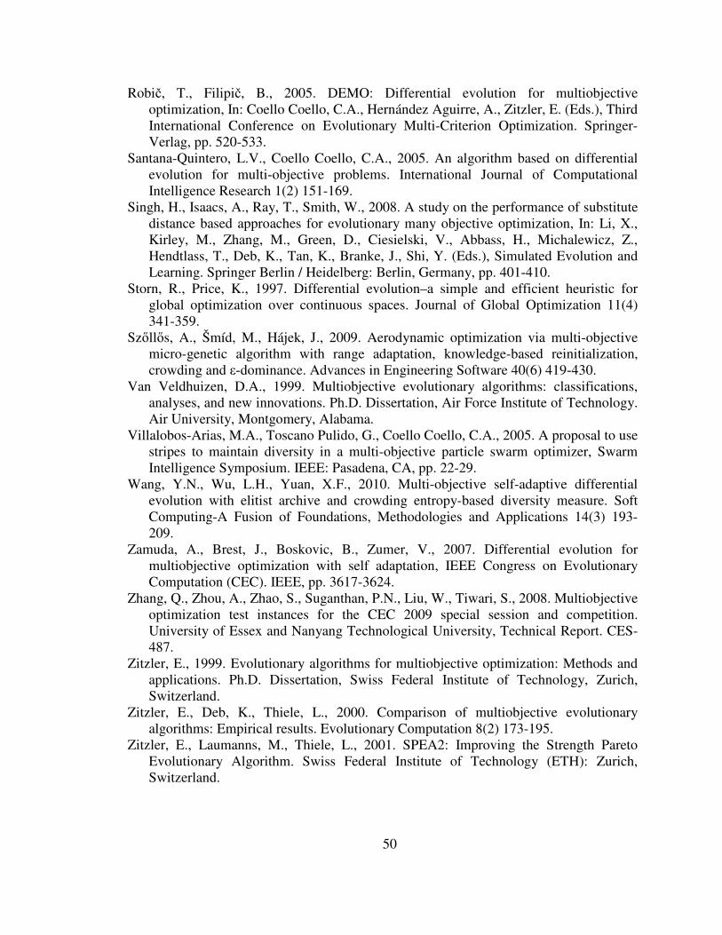
50

Robič, T., Filipič, B., 2005. DEMO: Differential evolution for multiobjective optimization, In: Coello Coello, C.A., Hernández Aguirre, A., Zitzler, E. (Eds.), Third International Conference on Evolutionary Multi-Criterion Optimization. Springer-Verlag, pp. 520-533.

Santana-Quintero, L.V., Coello Coello, C.A., 2005. An algorithm based on differential evolution for multi-objective problems. International Journal of Computational Intelligence Research 1(2) 151-169.

Singh, H., Isaacs, A., Ray, T., Smith, W., 2008. A study on the performance of substitute distance based approaches for evolutionary many objective optimization, In: Li, X., Kirley, M., Zhang, M., Green, D., Ciesielski, V., Abbass, H., Michalewicz, Z., Hendtlass, T., Deb, K., Tan, K., Branke, J., Shi, Y. (Eds.), Simulated Evolution and Learning. Springer Berlin / Heidelberg: Berlin, Germany, pp. 401-410.

Storn, R., Price, K., 1997. Differential evolution–a simple and efficient heuristic for global optimization over continuous spaces. Journal of Global Optimization 11(4) 341-359.

Szőllős, A., Šmíd, M., Hájek, J., 2009. Aerodynamic optimization via multi-objective micro-genetic algorithm with range adaptation, knowledge-based reinitialization, crowding and ε-dominance. Advances in Engineering Software 40(6) 419-430.

Van Veldhuizen, D.A., 1999. Multiobjective evolutionary algorithms: classifications, analyses, and new innovations. Ph.D. Dissertation, Air Force Institute of Technology. Air University, Montgomery, Alabama.

Villalobos-Arias, M.A., Toscano Pulido, G., Coello Coello, C.A., 2005. A proposal to use stripes to maintain diversity in a multi-objective particle swarm optimizer, Swarm Intelligence Symposium. IEEE: Pasadena, CA, pp. 22-29.

Wang, Y.N., Wu, L.H., Yuan, X.F., 2010. Multi-objective self-adaptive differential evolution with elitist archive and crowding entropy-based diversity measure. Soft Computing-A Fusion of Foundations, Methodologies and Applications 14(3) 193-209.

Zamuda, A., Brest, J., Boskovic, B., Zumer, V., 2007. Differential evolution for multiobjective optimization with self adaptation, IEEE Congress on Evolutionary Computation (CEC). IEEE, pp. 3617-3624.

Zhang, Q., Zhou, A., Zhao, S., Suganthan, P.N., Liu, W., Tiwari, S., 2008. Multiobjective optimization test instances for the CEC 2009 special session and competition. University of Essex and Nanyang Technological University, Technical Report. CES-487.

Zitzler, E., 1999. Evolutionary algorithms for multiobjective optimization: Methods and applications. Ph.D. Dissertation, Swiss Federal Institute of Technology, Zurich, Switzerland.

Zitzler, E., Deb, K., Thiele, L., 2000. Comparison of multiobjective evolutionary algorithms: Empirical results. Evolutionary Computation 8(2) 173-195.

Zitzler, E., Laumanns, M., Thiele, L., 2001. SPEA2: Improving the Strength Pareto Evolutionary Algorithm. Swiss Federal Institute of Technology (ETH): Zurich, Switzerland.

51

Chapter 3: Minimization of Cost, Sediment Load, and Sensitivity to

Climate Change in a Watershed Management Application

Abstract

One challenge of climate change adaptation is to design watershed-based

stormwater management plans that meet current total maximum daily load targets and

also take into consideration anticipated changes in future precipitation patterns. We

present a multi-scale, multiobjective framework for generating a diverse family of

stormwater best management practice (BMP) plans for entire watersheds. Each of these

alternative BMP configurations are non-dominated by any other identified solution with

respect to (i) cost of the implementation of the management plan, (ii) sediment loading

predicted at the outflow of the watershed, and (iii) sensitivity to predicted changes in

precipitation patterns. We first use GIS data to automatically precompute a set of cost-

optimal BMP configurations for each subwatershed, over its entire range of possible

treatment levels. We then formulate each solution as a real-valued vector of treatment

levels for the subwatersheds and employ a staged multiobjective optimization approach

using differential evolution to generate sets of non-dominated solutions. Finally, selected

solutions are mapped back to the corresponding preoptimized BMP configurations for

each subwatershed. The integrated method is demonstrated on the Bartlett Brook mixed-

used impaired watershed in South Burlington, VT, and patterns in BMP configurations

along the non-dominated front are investigated. Watershed managers and other

stakeholders could use this approach to assess the relative trade-offs of alternative

stormwater BMP configurations.

52

3.1 Introduction

Land use development for residential, commercial, industrial, and agricultural

purposes dramatically changes the surface hydrology of the landscape. Increases in

impervious area and decreases in vegetation can cause large increases in stormwater

runoff, resulting in increased erosion and transport of sediment and soil contaminants into

surface water bodies. Even the relatively rural state of Vermont has 107 impaired water

bodies. Of these, 17 are stormwater-impaired rivers and streams (VTDEC, 2010), which

means their total maximum daily pollutant load (TMDL) exceeds the standards set by the

Clean Water Act (USEPA, 2012) under current precipitation patterns. To mitigate

problems caused by non-point source impacts from developed lands, structural Best

Management Practices (BMPs) such as detention ponds and rain gardens can be installed

to reduce peak storm flows and remove pollutants from stormwater runoff.

Decisions about what types, sizes, and locations of BMPs will best manage

stormwater runoff are some of the most important challenges facing urban resource

managers, developers, and the public. These decisions often take years or decades to play

out and, in the past, have occurred in piecemeal fashion with little forward planning.

These ad hoc experiments are expensive and there is very little concrete empirical

evidence that the collection of BMPs installed in large urban watersheds actually meet

the intended goals to reduce total contaminant loading (Booth et al., 2002). Thus, the

regulating and regulated communities are faced with several challenges that include

uncertainty about collective BMP performance, lack of long-term monitoring data at the

watershed level, paucity of funds to either support additional research or install expensive

53

BMPs that may be unnecessary, and a need to do something now rather than ten years in

the future.

Determining the appropriate number, types, placement, and sizing of BMPs is a

complex constrained multiobjective optimization problem in which engineers seek to

simultaneously minimize surface water sediment load (and associated pollutants) and the

financial cost of BMPs that can be feasibly accommodated by the geography and land-

use patterns (Perez-Pedini et al., 2005). To further complicate the matter, good

watershed-based stormwater management plans should be robust to anticipated (but

uncertain) changes in precipitation patterns as the global climate changes (Milly et al.,

2008), even though this is not required by law. There are also social and political issues

associated with the placement of structural BMPs, so finding a single BMP configuration

that meets TMDLs in a cost-efficient manner is not sufficient. One approach is to utilize

modeling and optimization techniques to identify sets of good solutions from a large

population of possible solutions. Computational time to solve these complex,

multiobjective problems becomes important when one recognizes that computational

resources may be limited and that there is often a need to run these models iteratively, as

the situation changes and as stakeholder resistance or acceptance evolves. In this

environment, a computationally efficient, inexpensive, transparent, and transferrable

framework to explore the costs and benefits of different BMP configurations is essential.

Multiple competing objectives in an optimization problem can be handled in

different ways. The simplest is to lump multiple objectives into one overall fitness metric

by making a weighted average of the separate objectives. However, the best weights to

54

use for each objective can be difficult to determine in advance (Coello Coello, 1999), and

the prespecified bias may not even be clear if the separate objectives are correlated.

Alternatively, a lexicographic approach can be taken, in which solutions are sequentially

optimized using one objective at a time. This can produce reasonable solutions when

there is a natural ordering of objective importance. However, by giving priority to one

objective over another, solutions that are near-optimal in one dimension and optimal in

the other are completely overlooked, and large parts of the feasible region remain

unexplored (Coello Coello, 1999). Both the lumped and lexicographic approaches to

multiobjective optimization thus require predetermination of how trade-offs between

objectives will be made and only provide watershed managers with a single solution.

However, the reality of designing stormwater management plans in the context of

political and social systems is that trade-offs between objectives ultimately require

human judgment and compromises between stakeholders. This can be facilitated by

generating a set of non-dominated solutions using true multiobjective optimization,

where a non-dominated solution is defined as one that outperforms each of the other

identified solutions in at least one objective (Coello Coello, 1999). Comparing solutions

along this so-called non-dominated front allows stakeholders to weigh the trade-offs

between the various objectives and to identify points of higher cost efficiency.

Evolutionary algorithms (EAs) are particularly well-suited to multiobjective

optimization since they are population-based methods that already maintain sets of

potential solutions. Every EA requires the following to be defined (Eiben and Smith,

2003): (i) the representation of a potential solution (genome), (ii) a selection mechanism

55

based on the quality of the solutions, and (iii) a means of reproduction with variation.

Starting from an initial (usually random) population of potential solutions, the EA

evolves successively fitter generations of solutions. Fitness-based selection can be

applied when choosing which population members will be allowed to reproduce (parent

selection) and/or when choosing which children will survive into the next generation

(survivor selection). Evolution is terminated when some convergence criterion is met

(e.g., fitness achieves some predetermined threshold, no improvement occurs within a

fixed number of generations, and/or some maximum number of generations is exceeded).

Several authors have used EAs to optimize BMP deployment for minimizing

pollutant runoff from agricultural sources (Arabi et al., 2006; Chatterjee, 1997; Chiu et

al., 2006; Gitau et al., 2004; Gitau et al., 2006; Jha et al., 2009; Maringanti et al., 2009;

Muleta and Nicklow, 2005; Panagopoulos et al., 2012; Rabotyagov et al., 2010;

Srivastava et al., 2002; Veith et al., 2003). These methods all assume that the majority of

pollutants run off from the cultivated land. However, the urban stormwater situation is

different. In urban settings, large impervious surfaces such as roadways and buildings

lead to storm flash and thus greater amounts of water running off the land and through the

waterways, increasing sedimentation from erosion at all levels (Walsh et al., 2005). In

addition, in contrast to agricultural BMPs, such as modifying cultivation practices, costly

structural BMPs are built to capture and retain this excess runoff. A few studies using

single-objective evolutionary optimization for designing urban stormwater management

plans to meet TMDLs also exist (Hsieh et al., 2010; Limbrunner et al., 2007; Perez-

Pedini et al., 2005; Zhen et al., 2004); these either minimize a weighted sum of both cost

56

and contaminant objectives or minimize cost subject to the constraint that the TMDL be

met, denying the watershed manager a set of trade-off solutions. True multiobjective

urban and mixed-use optimization applications have more recently gained attention (Lai

et al., 2007; Lee et al., 2012). These existing methods require watershed managers to a

priori identify potential BMP locations in the watershed (since they cannot, for example,

be placed on developed land) and predesign those BMPs to either a fixed size, or a

limited number of fixed sizes. Every method referred to above uses discrete-valued

representations for decision variables; i.e., a given BMP is either applied at its

predetermined position or it is not. Only Rabotyagov et al. (2010) have attempted to find

solutions resilient to variable precipitation patterns, albeit by finding only a single

minimal cost solution that meets the TMDL under every one of a series of historical-

based precipitation patterns. To our knowledge, no one has attempted to find solutions

resilient to the increased intensity of precipitation anticipated due to climate change.

In this paper, we describe a general computationally efficient framework for

evolving non-dominated sets of potential BMP plans, thus providing watershed managers

and other stakeholders a means of assessing trade-offs between the various objectives.

Specifically, we employ a multiscale decomposition of the problem using GIS data to

determine the maximum feasible numbers and sizes of different types of BMPs that can

be placed in each subwatershed (Section 3.2.1). This enables us to precompute

subwatershed level optimizations over the entire range of feasible treatment levels and

formulate the watershed level solutions as real-valued vectors that are easily kept in the

feasible region and can be optimized using a multiobjective form of differential

57

evolution, a particularly efficient type of evolutionary algorithm (Section 3.2.2). We

develop computationally efficient measures of fitness for the three objectives of cost,

sediment load, and sensitivity of the watershed-based stormwater management plan to

expected increases in precipitation intensity, including the optional use of a rapidly

computable hydrologic surrogate for sediment load (Section 3.2.3). The proposed

computational framework is demonstrated on a model of the stormwater-impaired

Bartlett Brook watershed, a small, suburban mixed-use watershed in South Burlington,

Vermont, USA (Section 3.3). We wrap up with a discussion of some of the important

findings and implications for climate change adaptation in watershed management

(Section 3.4).

3.2 Methods

The overall framework is outlined in Figure 3.1 and described in the following

subsections. Although we demonstrate the method using specific choices of the

hydrologic model and multiobjective EA, other models and EAs could be substituted, if

desired.

3.2.1 Multiscale decomposition of potential solutions

The specific configuration of the BMP used in each subwatershed (i.e., its type

and design parameters) must somehow be encoded in the genome of each potential

solution. The individual and combined values of the design parameters for stormwater

BMPs are subject to physical and geographic constraints that place practical limits on

their geometry. For example, there are minimum and maximum feasible bounds on

various BMP dimensions that may vary by subwatershed. Second, as a practical

58

constraint, some types of BMPs, e.g., detention ponds, cannot be placed in areas that are

already developed. Third, some types of BMPs may be preferable in certain settings. For

example, rain gardens, while generally of smaller maximum capacity than detention

ponds, are both safer and more aesthetically pleasing, and are thus often preferred in

residential settings (Freeborn et al., 2012). Finally, the combined areas of all BMPs must

fit within the maximum treatable area of each subwatershed, which can be limited by

land use and land characteristics, as well as landowner preferences.

Figure 3.1: Overview of framework to find watershed-based stormwater management solutions.

There are several possible representations of these decision parameters in the

genome of an EA. At one extreme, the presence or absence of single fixed-size BMPs of

different types could be evolved for all subwatersheds, allowing the BMPs for each

subwatershed to be encoded in a few bits (as many as there are BMP types). This

approach was taken by Veith et al. (2003), Arabi et al. (2006), Gitau et al. (2006), and

Maringanti et al. (2009), but is too inflexible to determine optimal designs in mixed-use

settings.

1. Create watershed model, divided into

subwatersheds

4. Precompute optimal BMP cost curves for

subwatersheds

5. Staged multi-objective evolutionary optimization on one precipitation pattern

2. Get subwatershed characteristics (e.g., land use) from GIS

3. Select management parameters and BMP

unit costs

6. Discard solutions dominated under

alternative precipitation pattern

8. Decode selected solution(s) to BMP

configuration

7. Evaluate tradeoffs in non-dominated solutions

to select possible solutions

9. Determine exact placement of BMPs within

each subwatershed

59

At the other extreme, one could encode all of the BMP parameters (e.g., type,

width, height, depth, side slope, etc.) for each BMP in the entire watershed. However,

this approach greatly increases the number of variables and the size of the search space of

the optimization problem and also necessitates significant on-line constraint handling due

to dependencies between these parameters.

To retain flexibility in the sizing and type of BMPs, we adopt an intermediate

approach using multiscale decomposition. After the watershed has been subdivided into S

subwatersheds (Figure 3.1, step 1), we precompute the cost-optimal feasible BMP

implementation plans (Figure 3.1, steps 2-4) across a range of area-based treatment

fractions, from no treatment up to the maximum treatable area for each subwatershed

(≤ 1), as detailed in Section 3.2.3.1. The solution representation used in the evolutionary

algorithm is thus simplified to a real-valued vector of length S, where the vector elements

represent the feasible treatment fractions of the S subwatersheds. This approach limits the

search space to the feasible region and thereby avoids the need for constraint handling

during the evolutionary process. Moreover, by adopting a real-valued representation one

can employ methods that exploit the local gradients in this continuous search space, such

as differential evolution (Storn and Price, 1997), a computationally efficient type of EA

specifically designed for evolving real-valued vectors that is described in the next

section.

3.2.2 Multiobjective evolution of watershed-scale solutions

A variety of evolutionary methods have been developed for multiobjective

optimization, most of which incorporate the concept of domination rank into their

60

selection procedures. The rank of a solution provides a convenient way to combine

fitness measurements from multiple objectives into a single metric for comparing the

relative quality of solutions. Two solutions are said to be of the same rank if neither

dominates the other; i.e., each outperforms the other in fitness for at least one objective

(Coello Coello, 1999). In a population of potential solutions, the set of solutions not

dominated by any other solutions are considered rank 1, and comprise the so-called non-

dominated front. The set of solutions that are only dominated by rank 1 solutions are

known as rank 2 solutions, and so on.

The most popular multiobjective evolutionary algorithm for optimizing two

objectives is the Non-dominated Sorting Genetic Algorithm (NSGA-II) (Deb et al.,

2002). While NSGA-II can accommodate real-valued vectors, differential evolution (DE)

(Storn and Price, 1997) has been shown to be preferable to genetic algorithms for

optimization of real-valued vectors. DE creates new potential solutions by computing

weighted differences of existing solutions, which enables it to naturally follow the

contours of the fitness landscape and automatically shift from global search (exploration)

to local search (exploitation) as the population converges. Compared to competing

approaches designed for real-valued optimization, DE is simple to implement, requires

relatively small populations, has low computational overhead per generation, requires

relatively few generations to converge to global optima in a variety of benchmark

problems, and performs well even in the presence of correlated decision variables and

noise (Price et al., 2005). Consequently, DE has rapidly gained traction in the

evolutionary computation community for real-valued optimization (see Das and

61

Suganthan, 2011 for a recent review) and several multiobjective versions of DE have

been proposed over the last decade (e.g., Abbass and Sarker, 2002; Ali et al., 2012; Babu

and Anbarasu, 2005; Iorio and Li, 2004; Kukkonen and Lampinen, 2005; Landa Becerra

and Coello Coello, 2006; Li and Zhang, 2009; Qian et al., 2012; Qu and Suganthan,

2011; Robič and Filipič, 2005; Zamuda et al., 2007), each with their own unique

strengths.

Because evaluating the efficacy of individual watershed-based stormwater

management plans requires hydrologic simulations that are computationally costly, it is

particularly important to limit the computational overhead of the evolutionary

optimization algorithm itself, making multiobjective DE an attractive option.

Furthermore, for stakeholders to adequately weigh trade-offs between solutions and

identify points of maximum cost efficiency, it is desirable to have solutions fairly evenly

spaced along the non-dominated front. Thus, for the evolutionary steps we used USMDE,

an efficient implementation of multiobjective DE that was specifically designed to

improve the uniformity of spacing of solutions along the final non-dominated front. We

refer the reader to Chichakly and Eppstein (2013) for a detailed description of the

USMDE algorithm, implementation, and validation on standard multiobjective

benchmark problems. However, we note that any multiobjective evolutionary algorithm

that is capable of optimizing real-valued vectors (including NSGA-II) could be used.

3.2.3 Objectives in the watershed management problem

We seek optimal BMP implementation plans (BMP configurations) that minimize

three objectives: (i) cost of implementing the BMP configuration, (ii) suspended sediment

62

load at the outflow of the watershed, and (iii) sensitivity of sediment load to anticipated

changes in intensity of precipitation events. Rather than simultaneously optimize all three

objectives, we break the evolution into stages (Figure 3.1, steps 5-6), to limit the problem

to two objectives at a time. First, we perform a multiobjective evolutionary search to

determine solutions that are non-dominated relative to the first objective and a

computationally efficient surrogate for the second objective. We then continue the

evolution using a more accurate estimate of the second objective. Finally, we discard

solutions that are dominated under the third objective (Figure 3.1, step 6). This staged

approach is justified because (i) preliminary experimentation indicated that different

precipitation patterns generally produced similar sets of non-dominated solutions relative

to cost and sediment load, indicating that post-processing (as opposed to further

evolution) for the third objective should be adequate, (ii) the desire to minimize cost

(which is constrained by budgets) and sediment load (which is required by law) take

priority over the desire to minimize sensitivity to climate change (which is not currently

required by law), so treating the latter objective lexicographically is justified,

(iii) including the third objective (minimizing sensitivity to increased intensity of

precipitation) in the evolutionary phase would require sediment loads to be calculated

twice for every individual in every generation, thus dramatically increasing

computational costs, (iv) restricting the evolutionary search space to two dimensions at a

time permits much smaller population sizes, thus saving considerable computation time,

and (v) when using a rank-based selection mechanism as we do here, evolving for more

than two objectives simultaneously can cause nearly the entire population to lie on the

63

non-dominated multidimensional surface from early in the evolution; with little or no

selection pressure, it is difficult to improve the location of the non-dominated front so the

optimization will stagnate.

3.2.3.1 Evaluating objective 1: Cost of watershed-scale solutions

We obtain publically available physical information about each subwatershed

from a geographical information system (GIS). Specifically, for each subwatershed we

determine the area, average gradient, predominant soil hydrogroup (USDA, 1986),

average infiltration rate, impervious area fraction, area of open undeveloped land

appropriate for detention pond placement, and the fraction of area occupied by single-

family lots, multi-family lots, commercial lots, and municipal open space (Figure 3.1,

step 2). Since Vermont regulations stipulate that that BMPs must be designed to capture

90% of annual storm events, we also ascertain the state’s regulation 90% precipitation

event for the region.

In the current work, we allow five types of BMPs that are commonly used in

mixed-use settings: four types of infiltrating rain gardens (for single-family lots, multi-

family lots, non-residential lots, and/or municipal open space) and non-infiltrating

detention ponds. Additional types of BMPs could be modeled, if desired. We estimate

local political and BMP-specific information (Figure 3.1, step 3), including (i) the

expected costs of the various types of BMPs – for simplicity, these were approximated as

lifetime costs per area (cpa), (ii) the expected fraction of the area of each land-use type

that is typically available for rain gardens of a given type (favail – this is not needed for

detention ponds, as discussed below), (iii) the minimum feasible size for each BMP type

64

(minfeasible), and (iv) the expected fraction of landowners willing to allow

implementation of BMPs of a given type (fadopt). This last parameter, being

sociopolitical, cannot be ascertained from GIS data; however, a watershed manager

should be able to reasonably approximate this value for their region. If the final solutions

prove unacceptable to the landowners, the watershed manager can vary the parameter and

run the optimization again.

Using the data and assumptions described above, it is straightforward to

precompute the optimal proportion of area in each subwatershed that should be treated

with each of the allowable BMP types, in order to achieve any specific amount of treated

area for the subwatershed. Specifically, for a subwatershed with total area A, we use a

greedy algorithm to precalculate the minimum-cost areas ai to be treated with each BMP

type i (here, the four types of rain gardens as well as detention ponds), as a function of

the fraction of the treated area T of the subwatershed, for all T ∈ [0,1]. The maximum

area available for rain gardens (areaavaili) is approximated from the area of the

subwatershed and the fraction of that area available for the given type of rain garden

(subwatershedarea ⋅ favaili). The maximum area available for detention pond

construction (areaavaili) is directly determined from geographical data. The resulting

optimal areas ai are subjected to additional constraints on the maximum area available

(areaavaili ⋅ fadopti) for treatment with each BMP type i, and the minimum feasible area

(minfeasiblei) for each BMP type i, below which construction does not make sense. The

minimum feasible area for a given BMP type is calculated independently for each

subwatershed, by feeding the minimum area treated by the BMP type into the BMP

65

design equations available in most state stormwater manuals (e.g., VTANR, 2002). More

formally, we solve:

( )( ) ( ) [ ]

( ) [ ]

⋅

<⋅=∈

∈∀⋅=

⋅ ∑∑

otherwise ,

,0 ,,0 subject to

1,0,such that , minarg

ii

iii

iii

i

i

i

iiFa

fadoptareaavail

eminfeasiblfadoptareaavailamaxamaxTa

TATTacpaTai

(3.1)

The resulting subwatershed-level cost curves can contain discontinuities and non-

monotonicity (as illustrated for a representative subwatershed in Figure 3.2). Preliminary

experimentation with the hydrologic simulator used in this study (described in Section

3.2.3.2) showed the simulation results are governed by a BMP’s total surface area but are

insensitive to specific BMP lengths or widths, so we hold the length fixed and vary only

the width.

Since, by this method, we precompute costs for all feasible levels of treatment at

the subwatershed level, on-line computation of watershed-level solutions during the

evolutionary process (in Figure 3.1, step 5) is trivial. Specifically, when evaluating the

fitness, we interpolate the precomputed subwatershed-scale cost curves with the evolved

fractions of treated area for each subwatershed, and then sum these interpolated

subwatershed-level costs. DE bounce-back (Price et al., 2005) ensures that evolving

solutions are constrained to be in the feasible range by ensuring that the values of all

vector elements are bounded by zero and the maximum treatable area fraction of each

corresponding subwatershed.

66

Figure 3.2: a) Sample genome for a sample watershed with seven subwatersheds. Each value in the genome represents the fractional area of that subwatershed that is to be treated by BMPs. b) Actual cost curve for the first subwatershed in the Bartlett Brook watershed. The discontinuity in the curve occurs at the point where it becomes feasible to use a more cost-efficient detention pond rather than a series of rain gardens. Each point on the curve is associated with a precomputed optimal BMP configuration. For example, to treat 40% of subwatershed 1 (white circle), we have predetermined that it is optimal to build a detention pond with a surface area of 940 m2. (The additional dimensions of the detention pond are detailed in Section 3.2.5.)

3.2.3.2 Evaluating objective 2: Sediment load of watershed-scale solutions

To estimate the sediment load of potential solutions (in Figure 3.1, step 5), one

must employ a physics-based hydrologic simulation program that is capable of modeling

the impacts of BMPs on flow and sediment load. Although one can choose any process-

based hydrologic simulator, we demonstrate the framework using the widely-used

Hydrological Simulation Program - Fortran (HSPF) (Bicknell et al., 2001). Even though

HSPF is not spatially explicit below the level of the subwatershed, one can define as

many subwatersheds as necessary to achieve the desired spatial resolution. We model one

aggregated rain garden per subwatershed (constructed by combining all individual rain

gardens placed in the subwatershed) and one aggregated detention pond per

0

20000

40000

60000

80000

100000

120000

140000

160000

0 0.2 0.4 0.6 0.8 1

Fraction Treated

Co

st

($)

0.4 0.1 0 0.51 0.3 1 0.8

1 2 3 4 5 6 7 subwatershed:

treatment:

a)

b)

940 m2 detention pond

67

subwatershed. Aggregated rain gardens are modeled to flow into the top of each

subwatershed’s associated stream segment, in keeping with HSPF practice (Bicknell et

al., 2001), while aggregated detention ponds are modeled to flow into the bottom of the

stream segment, where they are typically installed.

Prior to the evolutionary optimization, we first define and calibrate an HSPF

model for the watershed in question (Figure 3.1, step 1). Sediment load for each evolved

BMP configuration can then be estimated by modifying this base HSPF model to include

the indicated BMPs and then simulating flow and sediment transport.

Modeling sediment load is computationally expensive relative to modeling

hydrologic flow, requiring more than twice the computation time in HSPF. This

computation time adds up quickly in an evolutionary algorithm, since the hydrologic

simulator must be run for each individual solution in the population, for each generation

in the evolution. In addition, when the entire optimization may need to be run multiple

times, most likely on desktop computers, computation time becomes even more

important. Thus, to reduce the computational cost of estimating sediment load, we elected

to use a previously validated sediment surrogate, standard deviation of flow (as described

in Chichakly, 2013), during the bulk of the evolutionary process in step 5 of Figure 3.1,

to rapidly identify promising areas of the search space. Once the front has converged

using this hydrologic surrogate for sediment as the second objective, the evolution is

resumed for a few additional generations using the more computationally costly HSPF

estimates of sediment load as the second objective, to refine the front and quantify

sediment load in the resulting solutions. For comparison, we also report on additional

68

tests in which we did not use the sediment surrogate at all, but evolved the initial front to

directly minimize cost and the more computationally costly prediction of sediment load.

We note that using this surrogate is optional in our framework; one can simply minimize

sediment load during the entire evolutionary process if sufficient computational resources

are available.

3.2.3.3 Evaluating objective 3: Robustness of watershed-scale solutions to more

intense precipitation

The effectiveness of BMPs depends on precipitation patterns (Semadeni-Davies et

al., 2008). Weather is inherently uncertain and variable, and climate change is

exacerbating this uncertainty. In the Northeastern United States, storm events are

expected to become more frequent with more variable intensity, although it is not clear

whether total precipitation will also increase (NECIA, 2006). Thus, to evolve solutions

that would be robust to potential changes in precipitation patterns, two precipitation

patterns are used during the evolutionary optimization: (i) an actual six-month

precipitation record is used to represent a typical current precipitation pattern and (ii) a

synthetic six-month precipitation pattern is generated to have the same total precipitation

as the actual precipitation record, but distributed into more frequent storms with greater

variation in their intensity. For the latter, we place a fixed number of storm events across

the entire season and vary their intensity randomly by up to plus or minus 50% from the

mean storm intensity (based on total precipitation and number of storm events). We

simulate the temporal shape of each storm, no matter its duration or intensity, as the Type

II Natural Resource Conservation Service (NRCS) 1-day design storm (USDA, 1983),

69

consistent with the typical shape for storm events in northern Vermont (USDA, 1986).

We follow the method described by Froehlich (2009, 2010) to generate the storms.

We first evolve solutions using one of these two precipitation patterns (Figure 3.1,

step 5). The solutions on the resulting non-dominated front are then reevaluated (and, in

some cases, further evolved for a few generations) using the other precipitation pattern,

as described in Section 3.2.3.4. Only those solutions that remain non-dominated relative

to cost and the change in resulting sediment load between the two precipitation patterns

are retained (Figure 3.1, step 6).

3.2.3.4 Experiments with order of objective evaluation

As described above, subsequent to the evolution of non-dominated solutions

relative to cost and the sediment surrogate (standard deviation of flow), we refine the

search to minimize with respect to (i) predicted sediment load and (ii) changes in

sediment load due to anticipated changes in precipitation patterns (Figure 3.1, steps 5-6).

However, there are several different orders in which these refinements can be applied and

it was not initially obvious which order is preferable.

We considered the four possible algorithm orders shown in Figure 3.3. In the first

three orders, we initially evolved the solutions to minimize cost and standard deviation of

flow (under one of the two precipitation scenarios) until the non-dominated first rank

solutions had converged to a stable front. We then switched to evolution with the more

computationally costly predictions of sediment load for a few more generations. In the

fourth order, we omitted the use of the surrogate and evolved to minimize cost and

sediment load until convergence. We subsequently switched to the precipitation scenario

70

not yet used, evolving further if needed. Regardless of which precipitation pattern was

applied first, we concluded with a final reevaluation of sediment load under the current

precipitation scenario, so current sediment loads could be compared to TMDLs. Finally,

we subtracted the sediment load under the more intense precipitation scenario from that

of the current precipitation scenario and retained only those solutions that were non-

dominated with respect to minimizing all three objectives (cost, sediment load, and

change in sediment load due to anticipated changes in precipitation).

Figure 3.3: Four possible orders for introducing computation of Sediment Load and the more Intense

Precipitation scenario into the evolution (implementation of steps 5 and 6 of Figure 3.1). The final front is then pruned to retain only solutions that are also non-dominated with respect to the estimated change in sediment load due to the difference in the intensity of the two precipitation scenarios (∆ Precipitation). See Section 3.2.3.4 for further explanation.

3.2.4 Using the non-dominated set of solutions

Once a set of non-dominated solutions has been achieved for a particular

watershed (Figure 3.1, Steps 1-6), stakeholders can assess the trade-offs between

Evolve (60 gens) Current Precipitation Sediment Surrogate

Evolve (15 gens) Current Precipitation

Sediment Load

Evolve (10 gens) Intense Precipitation

Sediment Load

Evolve (60 gens) Current Precipitation Sediment Surrogate


Sediment Surrogate


Sediment Load

Evaluate Current Precipitation

Sediment Load


Sediment Surrogate


Sediment Load


Sediment Load


Sediment Load


Sediment Load

Order 1 Order 2 Order 3 Order 4


Sediment Load

Prune based on ∆ Precipitation




71

objectives and select one (or more) desirable solutions for further consideration (Figure

3.1, step 7). After promising solution(s) have been identified, the treatment fractions of

these solutions can be easily translated back into the known proportions of treatment by

each BMP type (here, rain gardens and detention ponds) associated with that value on the

subwatershed cost curve (Figure 3.1, step 8). Once such a watershed-level solution has

been selected for implementation, watershed managers, developers, and other

stakeholders can negotiate the exact sizes and locations of detention ponds and rain

gardens within each subwatershed, based on practical and political considerations (Figure

3.1, step 9).

3.2.5 Bartlett Brook case study

This framework (Figure 3.1, steps 1-8) is illustrated on the stormwater-impaired

Bartlett Brook Watershed in South Burlington, VT, USA. Bartlett Brook drains a gently-

sloping, 2.85 km2 mixed-use watershed, containing three housing developments, a

commercial district along U.S. Route 7, and two farms. Roughly 30% of the watershed is

devoted to agriculture, 17% is wooded, 13% is open space associated with developments,

and the remaining 40% is developed (Figure 3.4). We built an HSPF model for Bartlett

Brook (Figure 3.1, step 1), subdivided into 14 subwatersheds whose boundaries were

provided to us by the Vermont Agency of Natural Resources (Figure 3.4). The model was

calibrated using five-minute precipitation and discharge data from 2006, excluding winter

months (Bowden and Clayton, 2010), with a Nash-Sutcliffe coefficient of 0.59. For the

evolutionary optimization, we used the 2008 five-minute precipitation pattern from

Bartlett Brook as the typical current precipitation pattern.

72

Figure 3.4: Bartlett Brook watershed with HPSF subwatershed delineations showing streams and subwatershed numbers (left) and showing land use across the subwatershed through a satellite image (right). The location of Bartlett Brook watershed within the state of Vermont is shown in the upper left.

The depth of all modeled rain gardens was fixed at 1.22 m (4 ft), the depth of all

modeled detention ponds was fixed at 2.74 m (9 ft), and both were modeled with side

slopes of 45°. The rain gardens were modeled with the same infiltration rate as the

surrounding land. Detention ponds were considered impermeable, with a 12.2 cm (4.8 in)

circular horizontal riser at 0.61 m (2 ft) and a broad-crested weir to control overflow at

2.74 m (9 ft). All of these parameters can be modified, and could even vary with

treatment level or BMP type (e.g., community rain gardens) if necessary, but the selected

values are consistent with accepted practice in the state of Vermont (VTANR, 2002) and

are sufficient to demonstrate the use of the framework. Table 3.1 shows the BMP-specific

estimates used in this study for detention ponds and rain gardens on single-family lots,

1

4

3

5

6 7

2

13

12

11

14

9 8

10

VT

Bartlett Brook

0 250 500 m

73

multi-family lots, commercial lots, and municipal open space (Figure 3.1, step 3). The

state of Vermont’s regulation 90% precipitation event for the region is 22.86 mm (0.9 in).

Table 3.1: BMP Parameters used to Derive Cost Curves for Bartlett Brook. Variable names match Equation (1): cpai: cost per unit area, favaili: fractional area typically available for constructing rain gardens, fadopti: expected fractional adoption rate by landowners. Costs are approximate lifetime averages.

i BMP type cpai ($/m2) favaili fadopti 1 Rain garden, single family 80.73 0.10 0.50 2 Rain garden, multi-family 80.73 0.05 0.75 3 Rain garden, non-residential 80.73 0.05 0.75 4 Rain garden, municipal 80.73 0.10 1.00 5 Detention pond 61.89 N/A 1.00

We demonstrate our approach using two precipitation patterns, one recorded

pattern from June to December of 2008 and a more intense precipitation pattern

consistent with climate change predictions. We note that we are not trying to find

solutions that meet the TMDL under these new conditions (as in Rabotyagov et al.,

2010), but rather we are trying to find solutions that are less sensitive (i.e., more robust)

to changing but uncertain conditions. For the Bartlett Brook watershed, the standard

deviation of recorded daily precipitation over the 2008 season was 6.63 mm/day, which is

almost identical to the standard deviation of a synthetic rainfall pattern with the same

total precipitation and same total duration but distributed in one-day storm events every

four days. Thus, to simulate a more intense precipitation pattern consistent with NECIA

(2006) predictions, we generated a synthetic rainfall pattern with the same amount of

total precipitation and same total duration but distributed in one-day storm events every

seven days, which exhibited a standard deviation of 8.51 mm/day (28% higher than the

2008 pattern).

74

For the Bartlett Brook application, we applied USMDE using a population of 60

individuals for all results reported here. (Population sizes of 40, 50, and 80 were also

tried; the smaller population sizes did not yield a sufficient density of solutions across the

non-dominated front while the population size of 80 added considerable computational

cost without a commensurate increase in the quality of the solutions.) The DE scaling

factor F was set to 0.6 and the crossover probability Cr was set to 0.2, in keeping with

recommendations in Price et al. (2005). In addition to using Latin hypercube sampling to

initialize the population with values distributed across the entire decision space, we also

added the two extremal solutions to the initial population (i.e., one solution with no

treatment, and one solution with maximum treatment of each subwatershed), to maximize

the spread along the non-dominated front.

3.3 Results of the Bartlett Brook case study

The effect of the four algorithm orders shown in Figure 3.3 on the resulting non-

dominated fronts for the Bartlett Brook watershed are shown in Figure 3.5. One “knee” is

apparent along these fronts. Solutions at a knee are the most cost-efficient, in that as one

moves along the front in either direction away from the knee, there are diminishing

returns in one objective with respect to the other (Figure 3.5a, b). Thus, solutions in this

region may optimize the trade-offs between objectives, assuming that the projected

sediment load of these solutions is within the required TMDL. In the high-cost region to

the left of the knee, the order 1 front had only one solution. The order 2 front had a

number of solutions in this high-cost region, but these (and the single order 1 solution)

were all dominated by the order 3 front. Not only did the order 3 front have much better

75

coverage than orders 1 and 2, but it was also the fastest (runtimes were 4.85 hrs, 4.65 hrs,

3.75 hrs, and 5.55 hrs using orders 1, 2, 3, and 4, respectively, on a 2 GHz Intel T7200),

requiring the fewest number of total generations than the other orders that used the

surrogate (70 generations for order 3 vs. 85 for orders 1 and 2). Note that the order 3

solutions lie directly on top of the non-dominated front found with order 4, which did not

use the sediment surrogate (Figure 3.5, solid line). To avoid confusion, we did not plot

the individual points for order 4, but we note that coverage of the front was similar

between orders 3 and 4, with the minor exception that the order 4 front contained 3

additional solutions above the knee.

2200 2400 2600 2800 3000 3200 3400 3600 3800 40000

2

4

6

8

10

12

x 105

sediment (t)

co

st

($)

"knee"

a

b

order 1 (generation 85)order 2 (generation 85)order 3 (generation 70)order 4 (generation 65)

Figure 3.5: Effect of algorithm order in moving from the sediment surrogate to sediment and to the high precipitation scenario. The orders match those listed in Figure 3.3. The ×s show the results for using order 1, the •s show the results for order 2, the +s show the results for order 3, and the solid line shows the front generated by order 4, running the more intense precipitation pattern and sediment load (not sediment surrogate). The triangle labeled a shows that above the knee increased expenditures lead to commensurately smaller decreases in sediment reduction. The triangle labeled b shows that below the knee increased expenditures lead commensurately larger increases in sediment reduction. Pollutant reduction is the most cost-efficient in the region of the knee.

76

When the precipitation pattern became more intense, all of the low-cost solutions

generated a larger (absolute and relative) increase in sediment load than did the high-cost

solutions (Figure 3.6). Under the more intense precipitation pattern, sediment load

increased by a factor of 1.47 for the highest cost solution, with the factor increasing

further to 1.57 for the lowest-cost (no treatment) solution. On the Bartlett Brook

watershed, only one of the non-dominated solutions in the order 3 front became

dominated when evaluated relative to objective 3 (change in sediment load due to change

in precipitation pattern), indicating that further evolution was not required for this

objective. Values for objectives 1 and 2 of the final order 3 solutions (non-dominated

under all three objectives) are also shown in Figure 3.6.

1600 1700 1800 1900 2000 2100 2200 2300 24000

2

4

6

8

10

12x 10

5

sediment (t)

co

st

($)

800 900 1000 1100 1200 1300 1400

change in sediment (t)

Robust Solutions

Sediment Differences

Figure 3.6: Robust sediment solutions (+s, bottom x-axis scale) and sediment differences under predicted precipitation pattern (•s, top x-axis scale) using order 3 (see Figure 3.3). Lower cost solutions generate proportionately more sediment under the predicted precipitation pattern than do higher cost solutions.

Selected solutions along the non-dominated front are depicted in Figure 3.7,

illustrating how the fraction treated in each subwatershed changes along the front. Not

77

surprisingly, as more of the watershed is treated by BMPs, more money is invested and

more sediment is removed. The fractions of the watershed treated by detention ponds

along the entire non-dominated front are shown in the Figure 3.7 inset (as determined by

Figure 3.1, step 8). The fractions of the watersheds treated by rain gardens (not shown)

are strongly positively correlated with the detention pond treatment fractions (r = 0.86),

but are an order of magnitude smaller; however, there is a discontinuity in this

relationship at a detention pond treatment fraction of about 0.8, where the rain garden

treatment fraction jumps from about 0.05 to greater than 0.07 and then remains fairly

high and approximately constant. This jump in rain garden fraction is what is responsible

for the "knee" in the non-dominated front (at around $620,000 cost) and causes the

visible change in slope in the cost curve in the Figure 3.7 inset, above which the BMP

configurations become less cost-efficient per unit sediment removed, since rain gardens

are more expensive. There is also a kink in the amount of sediment removed as a function

of detention pond treatment fraction for BMP configurations with sediment loads of

about 1700 t. Above this kink, rain garden treatment fraction remained relatively high

and constant, implying that the additional areas treated by detention ponds in these

highest cost configurations were less effective in removing sediment. On closer

inspection, we observed that these less effective detention ponds were installed in

subwatersheds with steeper slopes (11 through 14), which is evident in Figure 3.7. In

Figure 3.8, we detail one of the solutions found near the knee (the one circled in Figure

3.7) with different treatments by each BMP type, varying by subwatershed, showing how

78

this solution is translated back to specific BMP configurations using the precomputed

cost curves (in Figure 3.1, step 8).

Figure 3.7: Treatment fraction by subwatershed for solutions along the non-dominated front. A darker color means more treatment in that subwatershed and a lighter color means less treatment in that subwatershed with white representing no treatment at all (see color bar, top right). The percentage of each subwatershed’s area treated by detention ponds is given after “dp” and the percentage treated by rain gardens is given after “rg.” The inset shows how the detention pond treatment fraction varies across the front; although only detention pond treatment fraction is shown in the inset, the cost axis refers to the cost of the entire BMP configuration, including both detention ponds and rain gardens.

0

200

400

600

800

1000

1200

sediment (t)

cost ($

000s)

1550 1750 1950 2150 2350

dp: 92 rg: 7.7

dp: 89 rg: 6.5

dp: 86 rg: 7.7

dp: 83 rg: 6.5

dp: 79 rg: 4.8

dp: 70 rg: 5.0

dp: 46 rg: 4.8

dp: 47 rg: 3.8

dp: 47 rg: 0.0 dp: 36

rg: 3.9 dp: 29 rg: 0.9 dp: 31

rg: 0.9

dp: 20 rg: 3.0

dp: 23 rg: 0.9 dp: 13

rg: 0.2

dp: 0.0 rg: 0.0

Fra

ctio

n T

reate

d

0.0

1.0

0.2

0.4

0.6

0.8

0 0.2 0.4 0.6 0.8 1

1600

1800

2000

2200

2400

Detention Pond Treatment Fraction

Sedim

ent (t

)

0 0.2 0.4 0.6 0.8 10

200

400

600

800

1000

Cost ($

000s)

sedimentcost

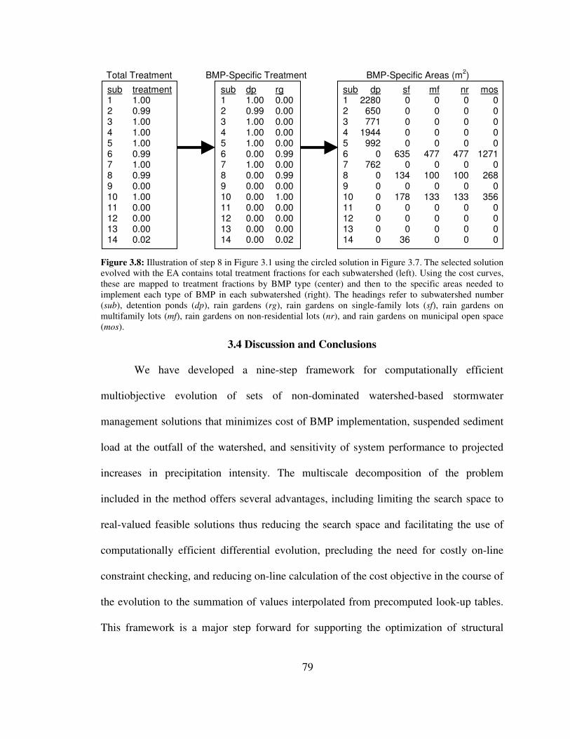
79

Figure 3.8: Illustration of step 8 in Figure 3.1 using the circled solution in Figure 3.7. The selected solution evolved with the EA contains total treatment fractions for each subwatershed (left). Using the cost curves, these are mapped to treatment fractions by BMP type (center) and then to the specific areas needed to implement each type of BMP in each subwatershed (right). The headings refer to subwatershed number (sub), detention ponds (dp), rain gardens (rg), rain gardens on single-family lots (sf), rain gardens on multifamily lots (mf), rain gardens on non-residential lots (nr), and rain gardens on municipal open space (mos).

3.4 Discussion and Conclusions

We have developed a nine-step framework for computationally efficient

multiobjective evolution of sets of non-dominated watershed-based stormwater

management solutions that minimizes cost of BMP implementation, suspended sediment

load at the outfall of the watershed, and sensitivity of system performance to projected

increases in precipitation intensity. The multiscale decomposition of the problem

included in the method offers several advantages, including limiting the search space to

real-valued feasible solutions thus reducing the search space and facilitating the use of

computationally efficient differential evolution, precluding the need for costly on-line

constraint checking, and reducing on-line calculation of the cost objective in the course of

the evolution to the summation of values interpolated from precomputed look-up tables.

This framework is a major step forward for supporting the optimization of structural

sub dp rg 1 1.00 0.00 2 0.99 0.00 3 1.00 0.00 4 1.00 0.00 5 1.00 0.00 6 0.00 0.99 7 1.00 0.00 8 0.00 0.99 9 0.00 0.00 10 0.00 1.00 11 0.00 0.00 12 0.00 0.00 13 0.00 0.00 14 0.00 0.02

sub treatment 1 1.00 2 0.99 3 1.00 4 1.00 5 1.00 6 0.99 7 1.00 8 0.99 9 0.00 10 1.00 11 0.00 12 0.00 13 0.00 14 0.02

sub dp sf mf nr mos 1 2280 0 0 0 0 2 650 0 0 0 0 3 771 0 0 0 0 4 1944 0 0 0 0 5 992 0 0 0 0 6 0 635 477 477 1271 7 762 0 0 0 0 8 0 134 100 100 268 9 0 0 0 0 0 10 0 178 133 133 356 11 0 0 0 0 0 12 0 0 0 0 0 13 0 0 0 0 0 14 0 36 0 0 0

Total Treatment BMP-Specific Treatment BMP-Specific Areas (m2)

80

BMP placement in the following ways: (i) only the maximum treatable area by each type

of BMP in each subwatershed needs to be predetermined; (ii) subwatershed treatment

fractions for each type of BMP are evolved using a real-valued representation that speeds

the search by implicitly constraining the search to the feasible region and permitting the

use of efficient optimization methods; (iii) exact BMP sizes and locations are only

established after first discovering how much area of a given subwatershed should be

treated with each type of BMP; this greatly simplifies the final sizing and placement

decisions and precludes the need to predesign BMPs before knowing if they will be

needed; and (iv) the final solution set is non-dominated with respect to cost, sediment

load, and sensitivity to more intense precipitation patterns, thus rendering them more

robust to climate change.

In this work, we have automated the individual steps 4, 5, 6, and 8 of the

framework. Step 1 has been partially automated by existing tools; e.g., BASINS from the

EPA. We suggest that steps 2, 3, and 9 could potentially be fully or partially automated,

as discussed more below. Ultimately, steps 1-6 and 8-9 would ideally be packaged into a

single, user-friendly software package, although this is beyond the scope of this

contribution. Step 7 (and probably also aspects of step 9) will always require stakeholders

to evaluate and negotiate tradeoffs between potential solutions.

Although we manually determined the inputs (steps 2 and 3) needed for the

precomputation of subwatershed-level cost curves (step 4), much of this work could be

automated. Specifically, we envision tools for: (i) automatic extraction of area, average

gradient, predominant soil hydrogroup, average infiltration rate, impervious area fraction

81

directly from GIS data; (ii) automatic extraction of the land use fractions used to

determine potential rain garden sites from the GIS land use overlay; (iii) automatic

extraction of potential detention pond sites from the GIS land use overlay; these will need

to be manually confirmed by the watershed manager before the optimization; and (iv)

automatic estimation of management parameters, BMP unit costs, and landholder

acceptance rates based on prior data.

Similarly, although we have not yet attempted to automate step 9, one could

conceivably implement an additional constrained evolutionary optimization, using fitness

based on a more spatially explicit hydrology model, to evolve placement and sizing of

specific BMPs within each subwatershed, subject to the treatment fractions for each BMP

type that were determined in step 8 for the solution(s) selected in step 7. This would

require several parameters per subwatershed, but because each subwatershed could be

optimized independently at this point, and because the feasible region of each of these

optimizations would be greatly reduced by the known treatment fractions required, this

would be much more efficient than trying to directly optimize at this level of detail for

the entire watershed. Even if such a software tool were developed that encapsulated steps

8-9, however, stakeholders would still likely need to have input into the final design

decisions for each subwatershed, possibly iteratively applying this tool with additional

constraints until a satisfactory solution is found.

Our results indicate that the standard deviation of flow can be an effective and

computationally efficient hydrologic surrogate for sediment load for the bulk of the

evolution of watershed-based stormwater management plans. As long as the more intense

82

precipitation pattern was applied first, we could not detect any loss in solution quality due

to the use of the sediment surrogate in place of the actual sediment load for the bulk of

the evolution, even though the evolution was faster when using the surrogate. Calculating

just the surrogate in the hydrology model runs 2.5 times faster than calculating sediment

load on this small watershed with only 14 subwatersheds. However, minimizing the

surrogate until convergence (60 generations) followed by minimizing sediment load for

an additional 10 generations ran only 1.5 times faster than minimizing sediment load until

convergence (65 generations). Nonetheless, the computational savings afforded by the

surrogate will be increasingly important for larger problems. While the absolute time

savings we observed in this study (3.75 hrs vs. 5.55 hrs) may not seem large, we

demonstrated the method on only 14 subwatersheds, simulated only six month scenarios,

and used a population size of only 60 individuals. Larger models with more

subwatersheds and longer simulation periods will afford a greater savings per fitness

evaluation by using the surrogate. Furthermore, the required population in EAs grows as

a function of the number of decision variables, so modeling more subwatersheds will

require larger populations. In addition, the optimization framework may need to be run

many times as stakeholders’ preferences change. However, we stress that the use of this

surrogate is an optional implementation detail.

We observed that whenever the algorithm switched from the current to the more

intense precipitation scenario, further evolution was necessary for the front to reconverge.

However, when switching from the more intense precipitation back to the current

precipitation scenario, further evolution did not affect the location of the front and was

83

therefore not required. Furthermore, starting with the more intense precipitation pattern

yielded many more solutions in the high-cost regions of the front that were also more

cost-efficient, i.e., provided better robustness for a lower incremental cost. This occurs

because high-cost solutions that provide adequate control of sediment loads generated by

the less intense precipitation pattern do not necessarily provide adequate control when

rain events become more intense, and thus often become dominated by cheaper solutions.

In contrast, solutions evolved to minimize sediment load under the more intense

precipitation pattern continue to be effective when precipitation becomes less intense, so

the high-cost region of the non-dominated front remains well-populated. Since higher-

cost solutions may need to be considered by watershed managers if lower-cost solutions

do not reduce sediment load below required TMDLs, or to develop solutions more robust

to climate change if financial resources permit, it is important to have good spread of

potential solutions along the entire front, even in high-cost areas.

Many multiobjective design problems include uncertainty in external forcing

conditions that may impact the optimality of various designs. When we first optimized

under the current precipitation scenario, we discovered many solutions became

dominated when we switched to the more intense precipitation scenario, for the reasons

described above. Our results suggest that, in general, to obtain a solution that is robust to

uncertain external conditions, it may be better to first optimize under stronger external

forcing conditions and then assess change in fitness under the weaker external forcing

conditions, although we have not tested this hypothesis on other problems.

84

Higher-cost solutions not only maximized reduction in sediment load, but were

also more robust to more intense precipitation patterns, generating proportionately less

additional sediment in the more intense precipitation scenarios than the lower-cost

solutions. Decision-makers should take this into account when selecting which solution to

implement, even if lower costs solutions would still meet current TMDLs, to avoid

construction of watershed-based stormwater management plans that rapidly become

inadequate as the climate changes. Unfortunately, our results for Bartlett Brook indicate

that sediment loads may increase by about 50% at the outfall of the watershed, even for

the most costly feasible management plans, if the intensity of precipitation events

increase as expected due to climate change in the Northeastern United States (NECIA,

2006), assuming the total amount of precipitation remains constant. Thus, it may not be

possible to meet TMDLs in the future without significant alterations to the watershed

characteristics (such as replacing impervious roadways and parking lots with pervious

surfaces).

As concerns regarding water quality and climate change continue to grow, it is

becoming increasingly important to develop watershed-based stormwater management

plans that not only satisfy current TMDLs, but are also as robust as possible to

anticipated changes in precipitation patterns. The computational methods described in

this paper automate much of this difficult process. Additional automation is possible and

would facilitate ready application to more sites. Use of this framework would provide

stakeholders and decision makers with the necessary information to adequately assess

trade-offs between competing objectives.

85

References



Arabi, M., Govindaraju, R.S., Hantush, M.M., 2006. Cost-effective allocation of watershed management practices using a genetic algorithm. Water Resources Research 42(10) W10429.

Babu, B.V., Anbarasu, B., 2005. Multi-objective differential evolution (MODE): an evolutionary algorithm for multi-objective optimization problems (MOOPs), The Third International Conference on Computational Intelligence, Robotics, and Autonomous Systems (CIRAS-2005): Singapore.

Bicknell, B.R., Imhoff, J.C., Kittle Jr, J.L., Jobes, T.H., Donigian Jr, A.S., 2001. Hydrological Simulation Program–Fortran, HSPF Version 12 User’s Manual. AQUA TERRA Consultants, Mountain View, California.

Booth, D.B., Hartley, D., Jackson, R., 2002. Forest cover, impervious-surface area, and the mitigation of stormwater impacts. Journal of the American Water Resources Association 38(3) 835-845.

Bowden, W.B., Clayton, M., 2010. Vermont stormwater flow monitoring project final report: 2006-2008, In: Vermont Agency of Natural Resources, S.S. (Ed.): Waterbury, Vermont.

Chatterjee, A., 1997. Watershed optimization of BMP implementation schemes using genetic algorithms. M.S. Thesis, Department of Agricultural and Biological Engineering. Pennsylvania State University, University Park, Pennsylvania.

Chichakly, K.J., 2013. Multiobjective design and innovization of robust stormwater management plans. Ph.D. Dissertation, Department of Computer Science. University of Vermont, Burlington, VT.

Chichakly, K.J., Eppstein, M.J., 2013. Improving uniformity of solution spacing in biobjective differential evolution, to appear in the Proceedings of the Genetic and Evolutionary Computation Conference (GECCO). ACM: Amsterdam, The Netherlands.

Chiu, S., Kuo, J., Hsieh, P., 2006. A model of optimal best management practices placement, World Environmental and Water Resources Congress 2006. ASCE: Omaha, Nebraska.

Coello Coello, C.A., 1999. A comprehensive survey of evolutionary-based multiobjective optimization techniques. Knowledge and Information systems 1(3) 129-156.



86

Eiben, A.E., Smith, J., 2003. Introduction to Evolutionary Computing. Springer-Verlag, Berlin, Germany.

Freeborn, J.R., Sample, D.J., Fox, L.J., 2012. Residential stormwater: Methods for decreasing runoff and increasing stormwater infiltration. Journal of Green Building 7(2) 15-30.

Froehlich, D., 2009. Mathematical Formulations of NRCS Design Storms. Journal of Irrigation and Drainage Engineering 135(2) 241-247.

Froehlich, D., 2010. Errata for “Mathematical Formulations of NRCS Design Storms” by David C. Froehlich. Journal of Irrigation and Drainage Engineering 136(9) 675-675.

Gitau, M.W., Veith, T.L., Gburek, W.J., 2004. Farm-level optimization of BMP placement for cost-effective pollution reduction. Transactions of the ASAE 47(6) 1923-1931.

Gitau, M.W., Veith, T.L., Gburek, W.J., Jarrett, A.R., 2006. Watershed level best management practice selection and placement in the Town Brook watershed, New York. Journal of the American Water Resources Association 42(6) 1565-1581.

Hsieh, P.H., Kuo, J.T., Wu, E.M.Y., Ciou, S.K., Liu, W.C., 2010. Optimal best management practice placement strategies for nonpoint source pollution management in the Fei-Tsui Reservoir watershed. Environmental Engineering Science 27(6) 441-449.


Jha, M., Rabotyagov, S., Gassman, P.W., 2009. Optimal placement of conservation practices using genetic algorithm with SWAT. International Agricultural Engineering Journal 18(1-2) 41-50.


Lai, F., Dai, T., Zhen, J., Riverson, J., Alvi, K., Shoemaker, L., 2007. SUSTAIN - An EPA BMP process and placement tool for urban watersheds, Water Environment Federation Conference. Water Environment Federation: Bellevue, Washington, pp. 946-968.


Lee, J.G., Selvakumar, A., Alvi, K., Riverson, J., Zhen, J.X., Shoemaker, L., Lai, F.-h., 2012. A watershed-scale design optimization model for stormwater best management practices. Environmental Modelling and Software 37 6-18.


Limbrunner, J., Vogel, R., Chapra, S., Kirshen, P., 2007. Comparison of linear and non-linear optimization models for storm water and non-point source pollution best

87

management practice decision support, World Environmental and Water Resources Congress 2007. ASCE: Tampa, Florida, pp. 1-10.

Maringanti, C., Chaubey, I., Popp, J., 2009. Development of a multiobjective optimization tool for the selection and placement of best management practices for nonpoint source pollution control. Water Resources Research 45(6) W06406.

Milly, P., Julio, B., Malin, F., Robert, M., Zbigniew, W., Dennis, P., Ronald, J., 2008. Stationarity is dead. Science 319 573-574.

Muleta, M., Nicklow, J., 2005. Decision support for watershed management using evolutionary algorithms. Journal of Water Resources Planning and Management 131(1) 35-44.

Northeast Climate Impacts Assessment (NECIA), 2006. Climate change in the US Northeast, A Report of the Northeast Climate Impacts Assessment. Union of Concerned Scientists Publications: Cambridge, Mass.

Panagopoulos, Y., Makropoulos, C., Mimikou, M., 2012. Decision support for diffuse pollution management. Environmental Modelling and Software 30 57-70.

Perez-Pedini, C., Limbrunner, J.F., Vogel, R.M., 2005. Optimal location of infiltration-based best management practices for storm water management. Journal of Water Resources Planning and Management 131(6) 441-448.




Rabotyagov, S.S., Jha, M., Campbell, T.D., 2010. Nonpoint-source pollution reduction for an Iowa watershed: An application of evolutionary algorithms. Canadian Journal of Agricultural Economics/Revue canadienne d'agroeconomie 58(4) 411-431.


Semadeni-Davies, A., Hernebring, C., Svensson, G., Gustafsson, L.-G., 2008. The impacts of climate change and urbanisation on drainage in Helsingborg, Sweden: Suburban stormwater. Journal of Hydrology 350(1–2) 114-125.

Srivastava, P., Hamlett, J., Robillard, P., Day, R., 2002. Watershed optimization of best management practices using AnnAGNPS and a genetic algorithm. Water Resources Research 38(3) 1021.


88

U.S. Department of Agriculture (USDA), 1983. Computer program for project formulation, National Resources Conservation Service Technical Release 20. United States Department of Agriculture: Washington, DC.

U.S. Department of Agriculture (USDA), 1986. Urban hydrology for small watersheds: TR-55, 2nd ed., National Resources Conservation Service Technical Release 55. United States Department of Agriculture: Washington, DC.

U.S. Environmental Protection Agency (USEPA), 2012. Introduction to the Clean Water Act. United States Environmental Protection Agency. http://cfpub.epa.gov/watertrain/pdf/modules/IntrotoCWA.pdf.

Veith, T.L., Wolfe, M.L., Heatwole, C.D., 2003. Optimization procedure for cost effective BMP placement at a watershed scale. Journal of the American Water Resources Association 39(6) 1331-1343.

Vermont Agency of Natural Resources (VTANR), 2002. The Vermont Stormwater Management Manual. Vermont Department of Environmental Conservation: Waterbury, Vermont.

Vermont Department of Environmental Conservation (VTDEC), 2010. 303(d) List of Waters, Part A – Impaired Surface Waters in Need of TMDL. Vermont Department of Environmental Conservation: Waterbury, Vermont.

Walsh, C.J., Roy, A.H., Feminella, J.W., Cottingham, P.D., Groffman, P.M., Morgan, R.P., 2005. The urban stream syndrome: Current knowledge and the search for a cure. Journal of the North American Benthological Society 24(3) 706-723.


Zhen, X., Yu, S., Lin, J., 2004. Optimal location and sizing of stormwater basins at watershed scale. Journal of Water Resources Planning and Management 130(4) 339-347.

89

Chapter 4: Discovering Design Principles from Dominated Solutions

Abstract

Important progress has been made by many researchers in extracting fundamental

design principles from patterns in design parameters along the non-dominated front

generated by evolutionary algorithms in biobjective optimization problems. However, to

our knowledge, no attention has been given to discovering design principles from the

wealth of additional information available from patterns in dominated solutions. To

explore that space, we use heatmaps of dominated solutions to visualize how relevant

variables self-organize with respect to the objectives throughout the feasible region. We

overlay ceteris paribus lines on these heatmaps to show how the objective values change

when a given design variable is varied while all others are held constant. We use three

biobjective optimization problems to demonstrate various ways in which these

visualization techniques can provide useful information beyond that which can be

determined from the non-dominated front. Specifically, we investigate a simple two-

member truss design problem, a simple welded beam design problem, and a real-world

watershed management design problem to illustrate (a) how principles derived from the

non-dominated front alone can be misleading, (b) how new principles can be derived

from the dominated solutions, and (c) how non-dominated solutions can often be fragile

with respect to assumptions about uncertain external forcing conditions, whereas

solutions a short distance inside the front are often much more robust.

90

4.1 Introduction

True multiobjective optimization, where multiple objectives are optimized

simultaneously, seeks a set of solutions that minimize (or maximize) multiple competing

objectives, in the sense that each solution in the set outperforms all other solutions in at

least one objective (i.e., are non-dominated). The resulting solution set forms what is

called the non-dominated front, sometimes referred to as the Pareto front if it is truly an

optimal set (Coello Coello, 1999).

Deb and Srinivasan (2006) introduced the term innovization to refer to the process

of examining patterns in decision variables along the non-dominated front to identify

fundamental design principles, thus deepening the understanding of a class of similar

problems. “Such…principles…should provide a reliable procedure of arriving at a ‘blue-

print’ or a ‘recipe’ for solving the problem in an optimal manner" (Deb and Srinivasan,

2006). This recipe can also be used to better inform the optimization process for related

problems. Whereas prior work focused on finding principles from the non-dominated

front exists (e.g., Deb, 2003; Obayashi and Sasaki, 2003), this was the first time a general

set of steps was proposed. The innovization process proceeds by finding an evenly-

spaced set of points along the non-dominated front, using a combination of single-

objective optimization, multiobjective evolutionary optimization, and local search. The

normal constraint method (Messac and Mattson, 2004), a numerical optimization method,

is then used to verify that the obtained front reasonably reflects the true Pareto front. The

resultant non-dominated front is analyzed to extract design principles. Deb and

Srinivasan (2006) applied their method to find design principles in several problems. For

91

example, they found that: (i) in a two-member truss design problem, all Pareto-optimal

solutions have equal stress on both truss members and also have a constant product of the

maximum stress on the truss and the volume of the truss members; (ii) in a multiple-disk

clutch brake design problem, increasing the number of disks monotonically improves

stopping action while increasing mass, and all Pareto-optimal solutions have the same

disk thickness and the same actuating force applied; (iii) in a spring design problem, all

Pareto-optimal solutions have the same spring stiffness; and (iv) in a welded beam design

problem, the thickness of the beam remains constant over most of the non-dominated

front while the shear strength of the material is the limiting factor in improving a solution

(all solutions on the non-dominated front have the maximum shear stress allowed).

Other methods for extracting design principles from non-dominated fronts have

also been proposed. Those that rely on visualization techniques (including the method we

propose here) are generally only applied to biobjective problems due to difficulties in

visualizing higher dimensional spaces, whereas those using clustering techniques have

also been applied to problems with more objectives.

Obayashi and Sasaki (2003), Chiba et al. (2006), and Doncieux and Hamdaoui

(2011) all used Kohonen self-organizing maps (SOMs) to extract design solutions from

the non-dominated front. SOMs are unsupervised neural networks that spatially separate

multidimensional data into groups that share similar characteristics, with closely related

groups arranged next to each other (Kohonen, 1990). SOMs automatically cluster data

with similar characteristics into groups (i.e., clustering), producing taxonomies of

solutions, thus finding semantic patterns in unordered data. Obayashi and Sasaki (2003)

92

successfully used SOMs to find patterns in the multiobjective solutions to two supersonic

transport aerodynamic problems, classifying both wing and fuselage designs. The SOM

was also used to classify the impact of the 131 different design variables on the

objectives, to find which ones had the greatest impact on overall performance. Similarly,

Chiba et al. (2006) used a SOM to find which design variables had the greatest impact on

shielding aircraft engine noise. Doncieux and Hamdaoui (2011) employed a SOM in the

design of a flapping wing aircraft to identify design variables that significantly affected

the velocity of the aircraft.

Ulrich et al. (2008) used dendrograms to hierarchically cluster non-dominated

solutions and then discover design principles. They develop a method to build the

dendrograms from a dataset and then applied their method to the design of a network

processor. Dendrograms are binary trees that represent organizational structures. The left

branch of each node has solutions that include the parent node’s characteristics while the

right branch has solutions that do not include the parent’s characteristics. The leaves of

the tree are the solutions themselves and nodes physically near each other generally share

common traits. The authors also vertically arranged the dendrogram nodes based on the

order in which the characteristics were selected, so that no two nodes had the same

distance from the root.

Askar and Tiwari (2011) presented an analytic approach for discovering the

Pareto front that leads directly to optimal design principles. They first establish the

boundaries of the decision space, defined by all constraints in the system. The boundary

points are connected with straight lines to define a region of feasible decision variables.

93

The (linear) equations for these lines are found in terms of the decision variables. Several

additional lines through the middle of the decision space are added to divide this region

into smaller pieces and their (linear) equations are found. Values along all of these lines

are substituted into the objective functions and dominated solutions are thrown out.

Additional lines through the region are added until the non-dominated front is well-

represented. The lines that lead to solutions on the non-dominated front are then used to

simplify the objective functions and the constraint functions and the resulting functions

are examined to find underlying design principles. The method is demonstrated on both a

welded beam design problem and a subwatershed stormwater drainage problem.

Brownlee and Wright (2012) highlighted solutions on the non-dominated front in

an Excel spreadsheet to more easily discern patterns. They used a translucent bar graph in

each cell to show the relative scale of each design variable, but reported that they found it

difficult to find patterns among the decision variables.

Kudo and Yoshikawa (2012) used isometric feature mapping (isomap) to extract

design principles in a hybrid rocket design problem. Like SOMs, isomap reduces high-

dimensional data into low-dimensional semantically-organized spatial patterns. For non-

linear data sets, isomap works better than either principal component analysis or

multidimensional scaling (Tenenbaum et al., 2000). Kudo and Yoshikawa (2012) created

an isomap that related the design parameters along the front to the resultant objective

values to help map design space to objective space and find patterns in the design

variables that led to different objective outcomes.

94

Ulrich (2012) used a biobjective evolutionary algorithm to partition both the

decision space and the non-dominated front into related clusters. The algorithm, Pareto-

Front Analyzer (PAN), locally optimizes every evolved solution before selection and has

specialized recombination and selection operators for populations of partitions. The

method successfully clustered similar designs in a truss bridge design problem.

Bandaru and Deb (2010, 2011a, b) developed an automated method to extract

design principles from non-dominated fronts. This method creates mathematical rules

that relate the decision variables, objective function values, and problem constraints. For

example, in the two-member truss design problem they found that S·V is constant along

the non-dominated front, where S is the maximum stress on the truss and V is the volume

of the truss. Similarly, in the welded beam design problem they found that d·L0.333 is

constant along the non-dominated front, where d is the deflection at the end of the beam

and L is the buckling load of the beam. This method depends on all solutions being very

close to the true Pareto front. Bandaru and Deb (2013) later extended their automated

methods to extract principles over prespecified regions of the non-dominated front (called

low-level innovization) and also across several non-dominated fronts discovered using

different problem parameters (called high-level innovization).

All of these prior innovization approaches have focused on extracting information

from solutions along the non-dominated front. However, to our knowledge, no attention

has been given to discovering design principles from the wealth of additional information

available from patterns in dominated solutions. In this paper, we introduce visualization

approaches to help identify patterns in dominated solutions across the fitness landscape of

95

biobjective design problems. These dominated solutions, precisely because they cover the

entire feasible region, give a much broader view of the impact of decision variables on

the objectives than do solutions on the non-dominated front alone, leading to greater

confidence that the derived design principles are truly fundamental and not just artifacts

of the front. Our results illustrate how patterns along the non-dominated front can

sometimes be misleading, how information present in dominated solutions can lead to

additional insights and design principles that cannot be determined from the non-

dominated front alone, and how visualizing sensitivity of variables across the feasible

region can help one to identify solutions that are more robust to uncertain external forcing

conditions.

4.2 Methods

In this section we describe our approaches to visualizing patterns in dominated

solutions of biobjective problems, followed by a description of the three design problems

we will use to illustrate these approaches.

4.2.1 Visualization Approaches

To visualize the space of dominated solutions, we follow these general steps:

1. Generate a variety of solutions throughout the feasible region as described in Section 4.2.1.1.

2. For particular variables of interest (e.g., design variables, constraints, aggregate metrics, and sensitivities of variables to changes in external forcing conditions): a. Generate a heatmap of the variable over the set of obtained solutions as

described in Section 4.2.1.2. b. For design variables, overlay ceteris paribus (cp) lines on the heatmap as

described in Section 4.2.1.3. c. Examine the heatmaps and cp lines to discover meaningful patterns within

the fitness landscape.

96

4.2.1.1 Populating the Feasible Region

To plot a heatmap of the feasible region, a sufficient number of potential solutions

(both non-dominated and dominated) must be found. In some cases, simply saving all

intermediate solutions from a biobjective evolutionary run may provide a sufficient

density of solutions to answer the questions at hand, especially if one only needs to

examine patterns in dominated solutions that are relatively close to the non-dominated

front. However, to obtain a more fully populated feasible region, we do the following:

1. Starting from random sets of solutions, we evolve towards the non-dominated front several times, saving all solutions from intermediate generations (Figure 4.1a).

2. Starting from random sets of solutions, reverse the objectives (i.e., if it’s a minimization problem, turn it into a maximization problem and vice-versa) and evolve towards increasingly dominated solutions several times, saving all solutions from intermediate generations (Figure 4.1b).

3. Generate additional random solutions as many times as needed to fill out the region between the non-dominated and fully-dominated fronts. If necessary, evolve these solutions a few generations in either direction until the entire region is adequately sampled, saving all intermediate solutions. In this work, we generated new solutions until we had a sufficient density for the desired level of spatial resolution in the heatmap (where we defined sufficient as having at least 10 solutions for each cell whose center lies within the region bounded by the non-dominated front and the fully-dominated front).

4. Remove infeasible solutions (i.e., those that do not meet the problem constraints) and duplicate solutions from the collected set of all solutions.

5. Check the density of cells and reapply steps 3 and 4 until the entire region is adequately sampled (Figure 4.1c).

For the evolutionary steps above, any biobjective evolutionary algorithm can be

applied. For this work we used USMDE (Chichakly and Eppstein, 2013), a

multiobjective version of differential evolution (DE) designed to explicitly encourage

uniformity of spacing along the front, with F = 0.6 and Cr = 0.2. Constraints were

97

handled using Constraint Adaptation with Differential Evolution (CADE) (Lampinen,

2002; Storn, 1999).

Figure 4.1: Development of heatmap of feasible region with cp lines for a representative problem. (a) Evolve toward the non-dominated front (bottom and left sides) multiple times, saving all intermediate solutions, (b) Reverse objectives and evolve toward dominated front (top and right sides) multiple times, saving all intermediate solutions, (c) Add random solutions until a desired density of solutions is achieved across the feasible region, (d) Evaluate a variable of interest (here, a design variable) in solutions across the feasible region, (e) Create a 2D moving average across the feasible region and display as a heatmap, and (f) Identify points (marked with black asterisks) to calculate cp lines from, and compute and overlay the cp lines (shown in white) on the heatmap.

4.2.1.2 Creating Heatmaps

It is difficult to directly identify patterns in these solutions due to heterogeneities

in nearby solutions (Figure 4.1d). Thus, we create two-dimensional (2D) heatmaps of

locally averaged solutions to permit visualization of patterns in the self-organized design

parameters (or other derived or aggregated variables) across the feasible solution set. We

first calculate a matrix (M) whose elements contain moving averages of associated

overlapping cells of the variable in question across the fitness landscape, at some pre-

98

specified level of spatial resolution. Elements in M that correspond to cells whose centers

lie outside the feasible region (i.e., beyond either the non-dominated front or the fully-

dominated front) are marked as infeasible. We then display the feasible region of M using

a pseudo-color plot (although any 3D visualization technique could be used – Figure

4.1e).

4.2.1.3 Creating the cp Lines

Ceteris paribus (cp) lines show where solutions will move in the feasible region

when exactly one of the design variables is changed. They are generated as follows:

1. From the moving-average matrix M of the variable in question, identify several places of interest to use as starting points (see asterisks on Figure 4.1f).

2. For each of these points: a. Extract the set of design variables from one solution inside the cell

associated with that point. b. Holding the other variables constant, re-evaluate both objectives at

evenly-spaced intervals across the allowable range of the variable of interest.

c. Plot the resulting curve on top of the heatmap, showing how the objectives change with the variable of interest (see lines on Figure 4.1f).

4.2.2 Visualizing Robustness to Uncertain Forcing Conditions

When external forcing conditions are uncertain, it is desirable to identify solutions

that not only balance the two primary objectives, but also maximize robustness to these

uncertain forcing conditions. Whereas one could conceivably add a third robustness

objective to the original optimization problem, adding this third objective would not only

significantly increase the computational burden of the evolutionary optimization but,

more importantly, would reduce the selection pressure among competing solutions (and

thus make it more difficult to find the Pareto optimal solutions) and would require many

99

more solutions to obtain adequate density and spacing along a 3D non-dominated surface.

Instead, we propose to create a set of 2D solutions as in Section 4.2.1.1 with respect to

the two primary objectives under one estimate of the forcing conditions, and then do the

following:

1. Re-evaluate all identified feasible solutions under one or more alternative estimate(s) of forcing conditions.

2. For each solution and for each performance objective of interest, find the maximum difference for that objective between these sets of forcing conditions.

3. For each objective of interest, generate a heatmap of the differences (i.e., a sensitivity map).

4.2.3 Test Problems Used

Three biobjective optimization problems illustrate the benefits of the proposed

visualization approach: (i) the design of a simple two-member truss, (ii) the design of a

simple welded support beam, and (iii) a watershed management design application. The

first two problems were selected because they have been used previously to demonstrate

innovization from the non-dominated front (Deb and Srinivasan, 2006) and are easily

understood, with only four design parameters each. The third problem is a complex

design problem that we have previously formulated as a biobjective optimization problem

(Chichakly et al., 2013), and is used here to illustrate how our visualization approaches

can provide valuable design insights for a real-world problem.

4.2.3.1 Two-Member Truss Design

This biobjective problem was originally studied in Chankong and Haimes (1983)

and is one of the problems analyzed by Deb and Srinivasan (2006). The problem is to

design a truss with two beams at minimal cost that can carry the specified load of 100 kN

100

without elastic failure. The volume of the truss members, which is linearly related to the

cost of the truss, is used as a proxy for cost. The maximum stress developed on either

member is minimized to avoid elastic failure. The original problem has three design

variables (Figure 4.2): AAC, the cross-sectional area of truss member AC (m2); ABC, the

cross-sectional area of truss member BC (m2); and y, the vertical distance from the

support structure (at A or B) to where the members join at C (m). To better demonstrate

our approach, we added a fourth design variable, xBC, the horizontal distance from B to C

(originally fixed at 1 m in Chankong and Haimes (1983)).

Figure 4.2: Two-member truss problem (after Chankong and Haimes, 1983)

The stress on each truss member AC and BC, named σAC and σBC, respectively, is:

σAC = 20xBC xAC

2 + y2

yAAC (1)

σBC = 20xAC xBC

2 + y2

yABC (2)

where xAC is the horizontal distance from A to C:

xAC = 5 – xBC (3)

C

A B

100 kN

y

xBC 5 m

101

The optimization problem is to minimize both cost (volume) of the truss and the

maximum stress on the truss:

cost(AAC, ABC, y, xBC) = AAC xAC2 + y2 + ABC xBC

2 + y2 (4)

max_stress(AAC, ABC, y, xBC) = max(σAC, σBC) (5)

subject to the following constraints:

max_stress ≤ 10 MPa

0 ≤ AAC, ABC ≤ 0.01 m2 (6)

0 ≤ y ≤ 3 m

0 ≤ xBC ≤ 2.5 m

Figure 4.3: Welded beam problem (after Deb and Srinivasan, 2006)

4.2.3.2 Welded Beam Design

Deb and Srinivasan (2006) present a biobjective problem of one beam being

welded to another to carry a load F (6000 lb) applied at the end of the beam. Both the

cost of the beam and the vertical deflection at the end of the beam must be minimized.

There are four design variables (see Figure 4.3): t, the width (or height) of the beam (in);

t

b

len h

6000 lbs

14 in

102

b, the thickness of the beam (in); h, the height (or thickness) of the weld (in); and len, the

length of the weld (in). The length of the beam is 14 + len inches.

The shear stress on the beam, τ, in psi, is defined by the following set of

equations:

τ = τ12 + τ2

2 + τ1τ2len

0.25(len2 + (h + t)2)

τ1 = 6000

2h⋅len (7)

τ2 = 6000(14 + 0.5len) 0.25(len

2 + (h + t)2)

2h⋅len

len

2

12 + 0.25(h + t)2

The bending stress on the beam, σ, in psi, and the buckling load on the beam, L, in

lb, are:

σ = 504000

t2b

(8)

L = 64746.022(1 – 0.0282346t)tb3 (9)

The optimization problem is to minimize both cost for the welded beam and the

vertical deflection at the end of the beam:

cost(b, t, h, len) = 1.10471h2len + 0.04811tb(14 + len) (10)

deflection(b, t, h, len) = 2.1952

t3b

(11)

103

subject to the following constraints:

τ ≤ 13600 psi

σ ≤ 30000 psi

b – h ≥ 0 (12)

L ≥ 6000 lb

0.1 ≤ t, len ≤ 10 in

0.125 ≤ b, h ≤ 5 in

4.2.3.3 Watershed Management Plan Design

Increases in impervious area and decreases in vegetation due to land use

development for residential, commercial, industrial, and agricultural purposes can cause

large increases in stormwater runoff, resulting in increased erosion and transport of

sediment and associated soil contaminants into surface water bodies. To mitigate

problems caused by non-point source impacts from developed lands, Best Management

Practices (BMPs) such as detention ponds and rain gardens can be installed to reduce

peak storm flows and remove pollutants from stormwater runoff. Some important

differences between rain gardens and detention ponds are that (a) rain gardens infiltrate,

whereas detention ponds do not, (b) rain gardens are more expensive per unit area than

detention ponds, (c) detention ponds have much larger minimum size requirements,

(d) rain gardens have stricter maximum slope restrictions, and (e) detention ponds cannot

be used in high density residential areas. Finding the optimal set of BMPs for any given

watershed is a complex problem. Chichakly et al. (2013) formulated this as a biobjective

design problem with real-valued design parameters, to minimize both cost and sediment

104

load through the optimal placement and sizing of BMPs within a mixed-use watershed.

Specifically, they used a multi-scale decomposition of the problem, where subwatershed-

level optimizations were pre-computed over the entire range of treatment options. The

evolutionary optimization problem was thus formulated such that the design variables

were simply the fraction of area that is treated in each subwatershed (referred to hereafter

as the treatment fraction). Evolved treatment fractions were then mapped back to pre-

computed optimal BMP configurations for each subwatershed.

The Bartlett Brook watershed in South Burlington, VT was divided into 14

subwatersheds provided by the Vermont Agency of Natural Resources and modeled

using Hydrological Simulation Program Fortran (HSPF) (Bicknell et al., 2001). Land-use

patterns were used to determine the maximum land area that could be used by each BMP

type within each subwatershed. The different costs and restrictions pertaining to rain

gardens and detention ponds cause nonlinearities and discontinuities in cost as a function

of area treated within the 14 subwatersheds. For example, if the area to be treated is less

than the minimum required for a detention pond, one is forced to use the more expensive

rain gardens to treat that area, whereas it is actually cheaper to install a detention pond to

treat a larger area. At the other end of the spectrum, if the area to be treated is larger than

the land available for detention ponds (e.g., due to residential development), then one

may need to supplement detention ponds with additional rain gardens. Chichakly (2013)

established a strong relationship between the logarithm of the standard deviation of flow

at the outfall and the logarithm of sediment load at the outfall (R2 values were above 0.87

for nine watersheds with varying characteristics). Thus, the biobjective optimization

105

problem was reframed to minimize cost and the standard deviation of flow at the outfall,

where the latter is an effective and computationally efficient proxy for sediment load at

the outfall, and that is the optimization problem we examine here.

Ideally, watershed management plans, which are expensive to implement and

difficult to change, will remain effective even as precipitation patterns change due to

global climate change. Already, rainfall patterns in the Northeastern U.S. are becoming

increasingly variable and uncertain, and climate change predictions are that the intensity

of individual rainfall events will continue to increase (NECIA, 2006). To partially

account for this, Chichakly et al. (2013), after biobjective minimization of cost and

standard deviation of flow, discarded solutions from the evolved front that were

dominated with respect to robustness to estimates of potential increased rainfall intensity.

This method helped identify which solutions on the non-dominated front were more

robust to potential changes in precipitation. Here, we apply the methods described in

Sections 4.2.1 and 4.2.2 to obtain greater insights into what factors make watershed

management plans more effective in removing sediment in a cost-efficient way and more

robust to increases in intensity of precipitation.

4.3 Results and Discussion

4.3.1 Truss and Beam Design

Selected two-member truss visualizations are shown in Figures 4.4-4.6 and

selected welded beam visualizations are shown in Figures 4.7-4.9. In each of these

figures, the left-hand panel shows how the selected variable changes along the non-

dominated front, while the right-hand panel illustrates how the same variable changes in

106

solutions across the feasible region. Although the feasible region for the welded beam

problem extends up to a maximum cost of $334 and a maximum deflection of 0.07 in, in

all figures for the welded beam problem (Figures 4.7-4.10) we have limited the displays

to a smaller region of interest near the non-dominated front. From these figures, it is

evident that contours in the heatmaps (i.e., bands of the same color) of the dominated

solutions in the feasible region can follow a variety of patterns. Specifically, for these two

design problems, we observed contours in these heatmaps that were roughly:

• Parallel to the y-axis: For example, in Figure 4.4b, it can be seen that over much

of the feasible region, decreases in the value of the plotted variable (AAC) are

associated with a large reduction in volume (x-axis) but with relatively little effect

on maximum stress (y-axis).

• Parallel to the x-axis: For example, in Figure 4.6b, over much of the feasible

region, increases in the value of the plotted variable (ABC) are associated with a

large reduction in maximum stress (y-axis) with relatively little effect on volume

(x-axis).

• Parallel to the non-dominated front: For example, in Figure 4.7b, the plotted

variable (t) increases in value as solutions near the non-dominated front.

• Non-monotonic: For example, in Figure 4.5b, over much of the feasible region,

the contours of the plotted variable (xBC) are roughly parallel to the y-axis (stress),

but the maximum values of the variable occur near the middle of the x-axis range

(volume), with values decreasing as one approaches either front (non-dominated

or fully-dominated).

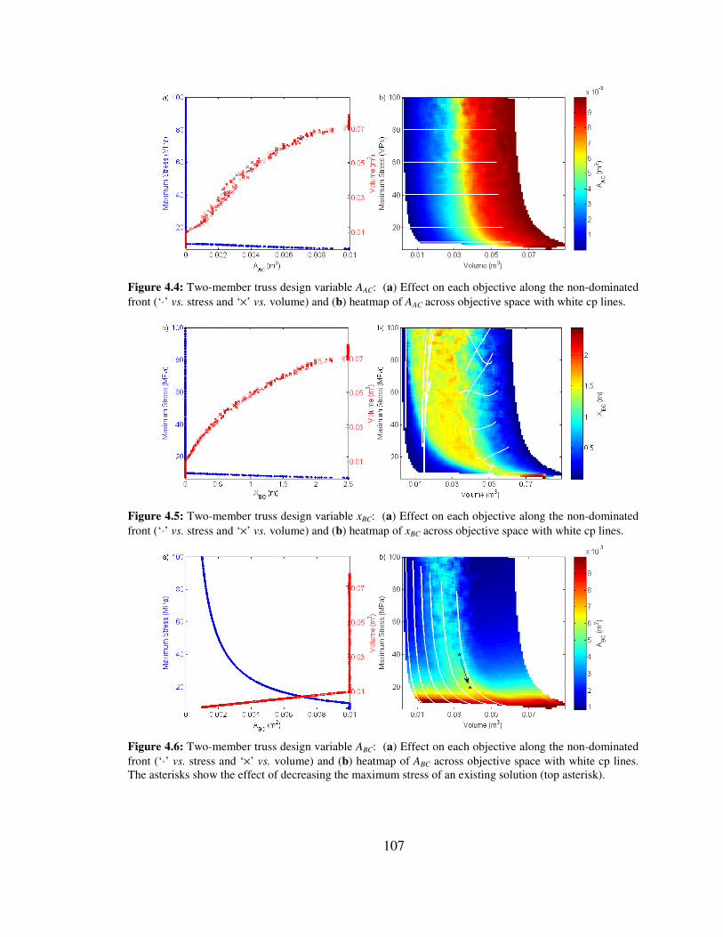
107

Figure 4.4: Two-member truss design variable AAC: (a) Effect on each objective along the non-dominated front (‘⋅’ vs. stress and ‘×’ vs. volume) and (b) heatmap of AAC across objective space with white cp lines.

Figure 4.5: Two-member truss design variable xBC: (a) Effect on each objective along the non-dominated front (‘⋅’ vs. stress and ‘×’ vs. volume) and (b) heatmap of xBC across objective space with white cp lines.

Figure 4.6: Two-member truss design variable ABC: (a) Effect on each objective along the non-dominated front (‘⋅’ vs. stress and ‘×’ vs. volume) and (b) heatmap of ABC across objective space with white cp lines. The asterisks show the effect of decreasing the maximum stress of an existing solution (top asterisk).

108

Figure 4.7: Welded beam design variable t: (a) Effect on each objective along the non-dominated front (‘⋅’ vs. deflection and ‘×’ vs. cost) and (b) heatmap of t across objective space with white cp lines.

Figure 4.8: Welded beam design variable h: (a) Effect on each objective along the non-dominated front (‘⋅’ vs. deflection and ‘×’ vs. cost) and (b) heatmap of h across objective space with white cp lines.

Figure 4.9: Welded beam design variable b: (a) Effect on each objective along the non-dominated front (‘⋅’ vs. deflection and ‘×’ vs. cost) and (b) heatmap of b across objective space with white cp lines.

109

In the following, we show how these visualized patterns, alone or in combination

with cp lines, can provide insights into various design problems.

Comparing Figures 4.4a-4.9a with the corresponding Figures 4.4b-4.9b, one can

see that inferences from solutions along the non-dominated front alone can be

misleading. For example, Figures 4.4a and 4.5a exhibit very similar relationships

between the maximum stress and cost objectives and the two-member truss variables AAC

and xBC, respectively, suggesting that volume can be reduced with minor impacts to

maximum stress by decreasing either of these variables. However, whereas the heatmap

and cp lines for AAC (Figure 4.4b) show that this design principle holds across the feasible

region, the heatmap and cp lines for xBC (Figure 4.5b) show that changes in xBC within the

dominated region produce very erratic results that behave very differently in different

parts of the dominated region.

The cp lines often provide additional information as to how to interpret the

heatmap. As in Figures 4.4a and 4.5a, Figures 4.8a and 4.9a exhibit very similar patterns

along the non-dominated front for the welded beam variables b and h, suggesting that a

decrease in either of these variables causes a decrease in cost and an increase in

deflection. In this case, however, the heatmaps for these two variables (Figures 4.8b and

4.9b) have similar contour patterns (almost parallel to the y-axis), indicating a decrease in

either variable results in a decrease in cost with little to no impact on deflection.

However, whereas the cp lines for h (Figure 4.8b) show that this relationship holds

throughout the feasible region, the cp lines for b (Figure 4.9b) show that decreasing b in a

110

dominated solution actually reduces cost and increases deflection, as was seen on the

front.

Likewise, in Figure 4.7a cost appears to be nearly independent of the welded

beam variable t, because t is close to its maximum value along the entire non-dominated

front. The heatmap shows contours for t that are parallel to the front (Figure 4.7b),

suggesting that increasing t would move one closer to the front by following this

gradient. However, the cp lines are actually nearly parallel to the front above the knee,

showing that increasing t yields major decreases in deflection for only minor increases in

cost over much of the feasible region; as deflection nears its minimum, one observes

diminishing returns for continuing to increase t, such that major increases in cost are

required for only minor decreases in deflection.

The non-dominated front shows that increasing the two-member truss variable

ABC will decrease maximum stress in a non-dominated solution up to a volume of 0.01 m3

(where ABC reaches its maximum) with a minor increase in volume (Figure 4.6a). There is

no useful information on the non-dominated front beyond a volume of 0.01 m3. Both the

heatmap and the cp lines in Figure 4.6b confirm that this pattern persists for larger

volume solutions as well. I.e., given any two-member truss design, it is possible to reduce

maximum stress in exchange for a relatively smaller increase in volume by increasing

ABC. As an illustration of this principle, suppose a manufacturer of two-member trusses

has a large inventory of trusses built for a specific application (as detailed in Section

4.2.3.1 and with a maximum stress of 40 MPa), but now wishes to modify these trusses

for use in a more demanding application (maximum stress of 20 MPa). The existing

111

trusses were built with design parameters AAC = 0.00747 m2, ABC = 0.00319 m2, y = 1.00

m, and xBC = 1.56 m, supporting the 100 kN load at the already specified maximum stress

of 40.0 MPa with a volume of 0.0327 m3 (top asterisk in Figure 4.6b). By increasing ABC

to 0.00637 m2, e.g., by welding a steel plate onto each existing member, the 50%

reduction in maximum stress to 20.0 MPa can be attained with an attendant increase in

volume of only 18% to 0.0386 m3 (bottom asterisk in Figure 4.6b).

For the welded beam variable h, the non-dominated front suggests that decreasing

h not only reduces cost, but also produces an attendant increase in deflection (Figure

4.8a). In contrast, the heatmap and cp lines show that reducing h actually reduces cost

with little to no change in deflection (Figure 4.8b). To illustrate this principle, suppose a

manufacturer of welded beams has an order for a large number of welded beams that

meet the specifications detailed in Section 4.2.3.2. From the evolved non-dominated

front, the manufacturer has picked a design with cost = $6.349 and deflection = 0.002896

in. The design parameters of the selected solution are b = 0.7581 in, t = 10.00 in, h =

0.6754 in, and len = 1.431 in. The variable h can be further reduced until the maximum

shear stress is reached (that is, when h = 0.6682 in). With this modification, deflection

remains unchanged (0.002896 in) while cost is reduced to $6.334, a 0.2363% savings,

relative to the originally selected solution on the evolved non-dominated front (which

could result in significant savings on large orders). This simplistic example serves to

prove the point that design principles learned from dominated solutions can actually be

used to push currently non-dominated solutions further towards Pareto-optimality.

112

In many engineering design problems, there is uncertainty in what the magnitude

of the external forcing conditions will be over the lifetime of the design. Although

properly designed beams are generally designed to handle maximum anticipated external

forcing conditions, the following simple example demonstrates how one can find

solutions that are more robust to uncertain forcing conditions. Suppose a manufacturer of

welded beams needs to design a beam that meets the conditions given in Section 4.2.3.2,

but, in a specific application, the beam may be subject to varying loads and there is some

uncertainty as to the true maximum load. Clearly, when the load exceeds the rated 6000

lb constraint, the stresses on the beam in solutions along the non-dominated front will

also increase beyond the allowable maximum. To find a design solution that is more

resilient to unexpectedly high loads, all solutions were re-evaluated with a 6,600 lb load

and a heatmap was created of the differences in both shear stress and bending stress

(Figure 4.10). Across the entire non-dominated front for shear stress, one observes that

moving a small distance inside the non-dominated front dramatically increases the

robustness of the sheer stress of the solution to changes in load (Figure 4.10a), i.e., the

differences in sheer stress decrease markedly. The inset of Figure 4.10a shows how

rapidly shear stress drops when moving orthogonally away from the non-dominated front,

starting from a representative point at the knee (cost = $7.43, deflection = 0.00275 in)

following the path of the white line. For example, if one instead implemented the solution

indicated by the circled point in the Figure 4.10a inset, for only a 9% increase in cost (to

$8.12) and an 11% increase in deflection (to 0.00306 in), the difference in shear stress

drops disproportionately by 23% (from 1330 psi to 1030 psi), making the beam much

113

more robust to variations in loading. On the other hand, bending stress in this same area

(along the white line in Figure 4.10b) is already at its maximum robustness.

Figure 4.10: Difference in shear stress (a) and bending stress (b) between applying a 6600 lb load at the end of the welded beam and the base case of applying a 6000 lb load. Inset graph (a) shows stress decreasing as move orthogonally away from the front at a representative part of the knee (x-axis of inset corresponds to points along the white line).

4.3.2 Watershed Management Plan Design

In Chichakly et al. (2013), non-dominated solutions to a complex watershed

problem were evolved to minimize cost of the BMP implementation plan and standard

deviation of flow at the outfall of the watershed. In the current work, we show how

valuable watershed management design principles can be discerned from patterns in

dominated solutions.

Three characteristic patterns appeared in the heatmaps and cp lines for the design

variables (i.e., subwatershed treatment fractions) of the Bartlett Brook watershed:

(a) Contours in the heatmaps for subwatersheds 1, 2, 3, and 5 were roughly parallel to the

non-dominated front above the knee, with treatment fraction increasing from right to left

exerting corresponding increases in sediment control (i.e., decreases in standard deviation

of flow) but with little impact on cost (e.g., Figure 4.11a); (b) Contours in the heatmaps

114

for subwatersheds 9, 11, 12, and 14 were roughly parallel to the non-dominated front

below the knee, with treatment fraction increasing from bottom to top incurring increases

in cost but relatively little effect on sediment control (e.g., Figure 4.11b); (c) Contours in

subwatersheds 4, 6, 7, 8, 10, and 13 exhibited a non-monotonic pattern where the

treatment fractions on the fully-dominated front are roughly a mirror-image of those

along the non-dominated front (e.g., Figure 4.11c). The cp lines close to the non-

dominated front were approximately orthogonal to the contours of the heatmaps in the

first two cases (e.g., Figures 4.11a and 4.11b), but are roughly parallel to the entire non-

dominated front in the third case (e.g., Figure 4.11c). Figure 4.12 shows heatmaps of all

14 design variables for the Bartlett Brook watershed. In this visualization, we have sized

each heatmap proportional to the area of its subwatershed, centered each heatmap

vertically at the mean elevation of its subwatershed, and showed how the subwatersheds

are connected based on drainage patterns. Those subwatersheds whose feasible solutions

contained only rain gardens are indicated with an asterisk.

Figure 4.11: Heatmaps with cp lines for three of the Bartlett Brook watershed design variables, illustrating the three types of observed patterns in dominated solutions. Specifically, the heatmaps represent the treatment fractions for subwatersheds (a) 1, (b) 9, and (c) 4.

115

Figure 4.12: Heatmaps of treatment fractions for all subwatershed in the Bartlett Brook watershed solutions, with associated subwatershed identification numbers and interconnections based on drainage topology (subwatershed 9 is at the outfall). Axes and color scale for each heatmap are identical to those shown in Figure 4.11. In this combined plot, the y-axis indicates the average elevation of each subwatershed (m), and each heatmap is sized proportional to the area of the subwatershed. Subwatershed numbers in bold with an asterisk next to them contain only rain gardens, whereas the other subwatersheds contain solutions using both detention ponds and (to a lesser degree) rain gardens.

Although the novel visualization in Figure 4.12 conveys a wealth of information

about each subwatershed, patterns yielding useful design principles governing treatment

fractions are still not immediately apparent. For example, there is no consistent

relationship between size of the subwatershed and its treatment fraction in feasible

solutions. One might initially conclude that it is more cost-efficient to treat larger

subwatersheds before smaller subwatersheds, since the smaller subwatersheds have little

to no treatment in solutions that are on or near the non-dominated front below the knee.

However, we observe very similar patterns in treatment fractions in subwatersheds 1 vs.

900

1200

1500

1800

2100

2400

2700 2

14 11

6*

7

9*

13

10*

1

3

12

5

4

8*

Ele

vatio

n (

m)

116

3, 2 vs. 5, and 4 vs. 7, even though the subwatersheds in each of these pairs are very

differently sized (Figure 4.12). Nor is mean subwatershed elevation a consistent

indication of the pattern of treatment fraction in feasible solutions. For example, note that

only four of the seven highest elevation subwatersheds (1, 2, 3, and 5) receive much

treatment in solutions that are on or near the non-dominated front below the knee. The

relative position between subwatersheds in the drainage topology is also not consistently

associated with patterns in treatment fractions. For example, subwatersheds 1, 2, 4, 5, and

12 are all at the top of the watershed, but exhibit different patterns in treatment fractions

across the feasible region, whereas subwatersheds 12 and 9 share very similar patterns

even though 12 is at the top of the watershed and 9 is at the bottom.

Plots of aggregate measures across the watershed proved more informative. For

example, we computed the total fraction of the watershed treated by detention ponds and

rain gardens in all feasible solutions. Not surprisingly, along the non-dominated front the

treatment fractions for both detention ponds (Figure 4.13a) and rain gardens (Figure

4.13b) increase from right to left, corresponding to more effective but more costly

management plans. In all solutions, the treatment fractions for detention ponds were an

order of magnitude higher than those for rain gardens. This occurs because, for a given

overall treatment fraction, our pre-computed subwatershed-level optimizations favored

the cheaper detention ponds over rain gardens, except where not possible due to

residential development. Thus, the heatmap for overall treatment fraction is visually

nearly identical to Figure 4.13a and is not shown.

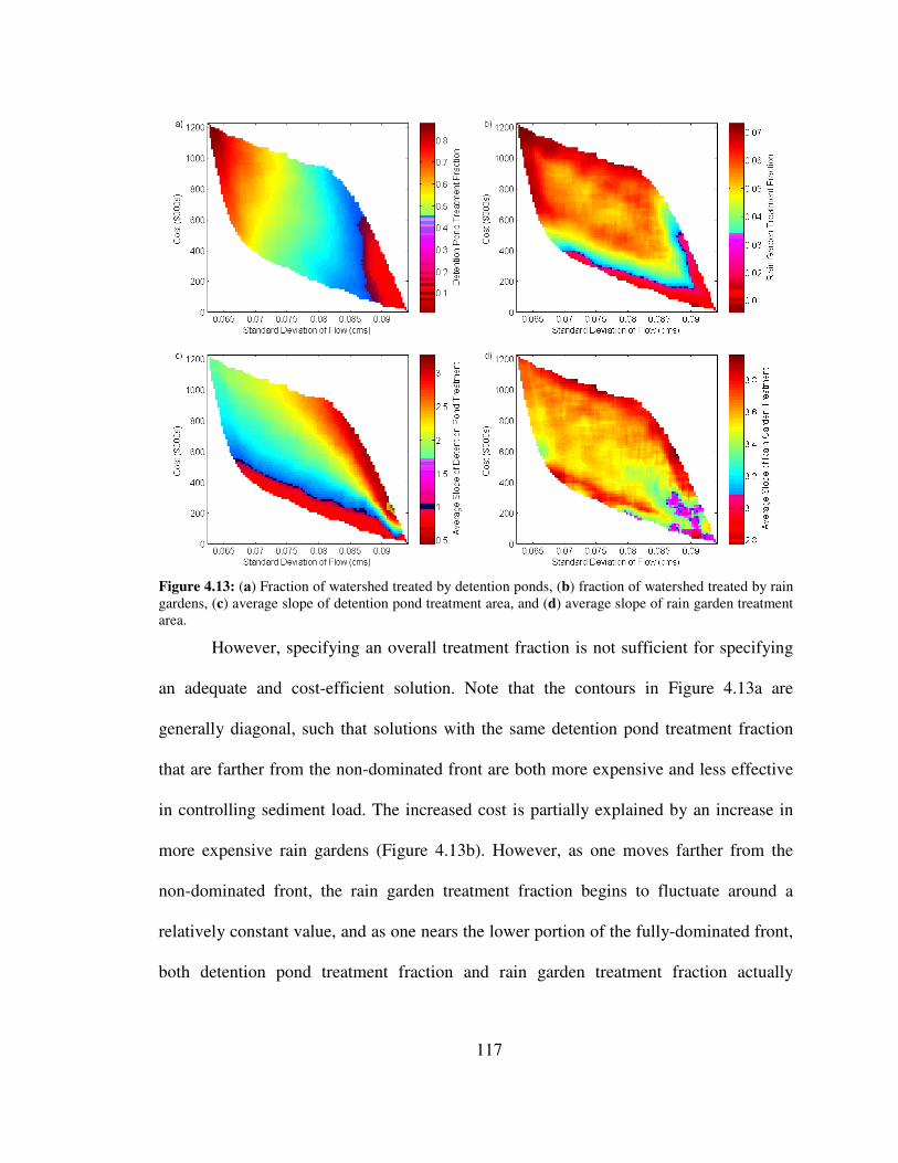
117

Figure 4.13: (a) Fraction of watershed treated by detention ponds, (b) fraction of watershed treated by rain gardens, (c) average slope of detention pond treatment area, and (d) average slope of rain garden treatment area.

However, specifying an overall treatment fraction is not sufficient for specifying

an adequate and cost-efficient solution. Note that the contours in Figure 4.13a are

generally diagonal, such that solutions with the same detention pond treatment fraction

that are farther from the non-dominated front are both more expensive and less effective

in controlling sediment load. The increased cost is partially explained by an increase in

more expensive rain gardens (Figure 4.13b). However, as one moves farther from the

non-dominated front, the rain garden treatment fraction begins to fluctuate around a

relatively constant value, and as one nears the lower portion of the fully-dominated front,

both detention pond treatment fraction and rain garden treatment fraction actually

118

decrease, yet the cost continues to increase (Figures 4.13a and 4.13b). This non-linearity

occurs due poor watershed management plans near the fully-dominated front that land at

high points in the non-linear subwatershed cost-per-area-treated functions.

Why are the most costly solutions with the same detention pond treatment

fractions less effective in controlling sediment load? Heatmaps of area-weighted

elevation and impervious area treated (not shown) exhibit the same pattern as detention

pond treatment fraction, so do not shed any additional light on this matter. However, a

heatmap of the weighted average of the slopes of the subwatersheds, weighted by the area

treated by detention ponds (Figure 4.13c) and rain gardens (Figure 4.13d) helps to

explain this. Comparing Figures 4.13a and 4.13c, it is immediately apparent that, for the

same detention pond treatment fraction, detention ponds on steeper slopes are less

effective. Thus, an inferred design principle is: Detention ponds on shallower slopes are

more effective in reducing sediment load. Although this principle was derived by

comparing treatment fractions between subwatersheds, it could also provide useful

guidance for specific placement of the actual detention ponds within each subwatershed.

The relationship between rain garden treatment fraction (Figure 4.13b) and slope

(Figure 4.13d) is less clear. Further investigation revealed that the subwatersheds selected

for treatment with rain gardens on or near the non-dominated front were subwatersheds 6,

8, and 10, where detention ponds were not feasible due to existing development.

119

Figure 4.14: Difference in pollutant load for different BMP treatments between a more intense precipitation pattern predicted by (NECIA, 2006) and the existing precipitation in Bartlett Brook. White lines indicate places where moving away from the front may produce a solution that is more resilient to changes in precipitation.

The watershed problem provides a more realistic application of design in the face

of uncertain forcing conditions. By law, states are only required to treat watersheds

sufficiently to meet contaminant targets under current precipitation patterns. However,

precipitation patterns in the Northeastern U.S. are expected to become increasingly

intense due to climate change (NECIA, 2006). It would therefore be wise to implement

plans today that are better able to manage the expected (but unknown) increased pollutant

loads in the future. Thus, to assess the robustness of solutions to anticipated increases in

intensity of precipitation, in Figure 4.14 we display the difference in standard deviation

of flow with respect to two different rainfall patterns, the actual rainfall pattern from

2008 and a more intense synthetic precipitation pattern with the same total precipitation

concentrated into more intense storms (specifically, with a standard deviation of rainfall

28% higher than the 2008 pattern; see Chichakly (2013) for more details). In several

120

places (see white lines on Figure 4.14), solutions a short distance away from the non-

dominated front were found to be more robust (i.e., show smaller increases in standard

deviation of flow in response to increases in the intensity of precipitation) than the

solutions on the front. For example, consider the solution close to the knee of the front, at

a cost of $327,000 and a standard deviation of flow of 0.0727 cms, marked with an

asterisk on Figure 4.14. The sensitivities to increased intensity of precipitation along the

horizontal and vertical white lines shown emanating from this point in Figure 4.14 are

plotted in Figures 4.15a and 4.15b, respectively. Moving horizontally there is a rapid

nonlinear drop in sensitivity by moving only a short distance; for example, if one is

willing to accept a small (2%) increase in the current standard deviation of flow, but one

is not willing to increase implementation costs, one can reduce the sensitivity by 4%

(Figure 4.15a, circled point). On the other hand, moving vertically, if one is willing to

increase the cost but is not willing to allow an increase in the current standard deviation

of flow, then one achieves only a linear decrease in sensitivity (Figure 4.15b);

specifically, each 4% increase in cost reduces the increase in future standard deviation of

flow by only 1%, so moving in this direction is less cost-effective. The corresponding

detention pond and rain garden treatment fractions along these two lines help explain the

reasons behind these decreases in sensitivity (increases in robustness) just inside the

front. As shown in Figures 4.15c and 4.15d, rain garden treatment fraction increases in

the more robust solutions; when cost is held constant, this is accompanied by a decrease

in detention pond treatment fraction (Figure 4.15), whereas when cost is allowed to

increase the detention pond treatment fraction also increases. These relationships also

121

hold along the other white lines in Figure 4.14. Since rain gardens infiltrate whereas

detention ponds do not, the increase in robustness from increased treatment with rain

gardens may be tied to increased infiltration. Thus, a design principle is: Whereas rain

gardens are less cost-effective for a given level of control, modest increases in the

proportion of rain garden treatment fraction, relative to detention pond treatment fraction,

may increase the robustness of the watershed to increases in the intensity of precipitation

events.

0.072 0.074 0.076 0.078−6

−4

−2

0

Standard Deviation of Flow (cms)

Diffe

rences (

perc

ent)

a)

300 350 400 450 500−15

−10

−5

0

Cost ($000s)

Diffe

rences (

perc

ent)

b)

0.072 0.074 0.076 0.0780.35

0.4

0.45

Standard Deviation of Flow (cms)

Dete

ntion P

ond T

reatm

ent F

raction

c)

0.072 0.074 0.076 0.0780.01

0.02

0.03

0.04

Rain

Gard

en T

reatm

ent F

raction

300 350 400 450 500

0.44

0.46

0.48

Cost ($000s)

Dete

ntion P

ond T

reatm

ent F

raction

d)

300 350 400 450 5000.01

0.02

0.03

0.04

0.05

Rain

Gard

en T

reatm

ent F

raction

Figure 4.15: Breakout of leftmost set of white lines from Figure 4.14, both with increasing standard deviation of flow (left) and increasing cost (right). The relative differences in standard deviation of flow between the two precipitation patterns are shown in the top row and the corresponding change in treatment fraction of each BMP type is shown in the bottom row.

4.4 Conclusions

We have shown that patterns in dominated solutions throughout the feasible

region can often give more information than is apparent from patterns along the non-

dominated front alone. By visualizing the inherent self-organization in design parameters

and other variables of interest across the feasible region, in relation to the non-dominated

122

and fully-dominated fronts, we can obtain sound insights into underlying design

principles that are valid throughout the entire design space.

With simple examples from a two-member truss design problem and a welded

beam design problem, we demonstrated that the information on the non-dominated front

can sometimes be misleading and that information from dominated solutions can provide

additional useful design principles. We also showed how these principles could be used

to modify and improve an existing design, and to improve a previously non-dominated

solution. Furthermore, in the welded beam problem, we discovered that dominated

solutions a short distance inside the non-dominated front exhibited markedly reduced

sensitivity of sheer stress to increased loading, with only minor degradations to the

solution quality with respect to the original objectives.

We also visualized patterns in dominated solutions of a complex watershed

management plan design problem. This helped us to discover that, for the same overall

treatment fraction, placing detention ponds in areas of the watershed with shallower

slopes reduces pollutant load at a lower cost. We also discovered that some solutions to

the watershed management problem, which were only slightly suboptimal with respect to

the original two objectives, were much more robust to increased intensity of precipitation.

Further visualizations revealed that this increase in robustness was due to a small increase

in the relative proportion of treatment by infiltrating rain gardens, relative to non-

infiltrating detention ponds. Such insights provide valuable guidance to watershed

managers who are required to develop management plans that can meet today’s

123

contaminant requirements, but will hopefully also remain as effective as possible as the

climate changes.

From the insights gained in these examples, we anticipate that visualization of

dominated solutions could lead to useful innovizations in a variety of biobjective

engineering design problems. Since the entire feasible region is included, identified

design principles remain valid across this entire region, thus enabling the improvement of

existing designs and ruling out apparent relationships that are artifacts of the non-

dominated front. In addition, we find that strictly non-dominated solutions are often

fragile, in the sense that they are only optimal with respect to the specific forcing

conditions for which they were evolved. Visualizing sensitivities to changes in these

forcing conditions across the feasible region can often help one identify solutions that are

much more robust to uncertainties in these assumptions.

References

Askar, S., Tiwari, A., 2011. Finding innovative design principles for multiobjective optimization problems. IEEE Transactions on Systems, Man, and Cybernetics, Part C: Applications and Reviews 41(4) 554-559.

Bandaru, S., Deb, K., 2010. Automated discovery of vital knowledge from Pareto-optimal solutions: First results from engineering design, IEEE Congress on Evolutionary Computation (CEC). IEEE, pp. 1-8.

Bandaru, S., Deb, K., 2011a. Automated innovization for simultaneous discovery of multiple rules in bi-objective problems, Evolutionary Multi-Criterion Optimization. Springer, pp. 1-15.

Bandaru, S., Deb, K., 2011b. Towards automating the discovery of certain innovative design principles through a clustering-based optimization technique. Engineering Optimization 43(9) 911-941.

Bandaru, S., Deb, K., 2013. Higher and lower-level knowledge discovery from Pareto-optimal sets. Journal of Global Optimization 1-18.


124

Brownlee, A.E., Wright, J.A., 2012. Solution analysis in multi-objective optimization, First Building Simulation and Optimization Conference. International Building Performance Simulation Association - England: Loughborough, UK, pp. 317-324.

Chankong, V., Haimes, Y., 1983. Multiobjective Decision Making: Theory and Methodology. North-Holland, New York.

Chiba, K., Imamura, T., Amemiya, K., Jeong, S., Yamamoto, K., 2006. Design exploration of shielding effect for aircraft engine noise. Transactions of the Japan Society for Aeronautical and Space Sciences.





Deb, K., 2003. Unveiling innovative design principles by means of multiple conflicting objectives. Engineering Optimization 35(5) 445-470.

Deb, K., Srinivasan, A., 2006. Innovization: innovating design principles through optimization, Genetic and Evolutionary Computation Conference (GECCO). ACM, pp. 1629-1636.

Doncieux, S., Hamdaoui, M., 2011. Evolutionary algorithms to analyse and design a controller for a flapping wings aircraft, In: Doncieux, S., Bredeche, N., Mouret, J.-B. (Eds.), New Horizons in Evolutionary Robotics. Springer: Heidelberg, pp. 67-83.

Kohonen, T., 1990. The self-organizing map. Proceedings of the IEEE 78(9) 1464-1480. Kudo, F., Yoshikawa, T., 2012. Knowledge extraction in multi-objective optimization

problem based on visualization of Pareto solutions, IEEE Congress on Evolutionary Computation (CEC). IEEE, pp. 1-6.

Lampinen, J., 2002. A constraint handling approach for the differential evolution algorithm, IEEE Congress on Evolutionary Computation (CEC). IEEE, pp. 1468-1473.

Messac, A., Mattson, C.A., 2004. Normal constraint method with guarantee of even representation of complete Pareto frontier. AIAA journal 42(10) 2101-2111.


Obayashi, S., Sasaki, D., 2003. Visualization and data mining of Pareto solutions using self-organizing map, Evolutionary multi-criterion optimization. Springer, pp. 71-71.

Storn, R., 1999. System design by constraint adaptation and differential evolution. IEEE Transactions on Evolutionary Computation 3(1) 22-34.

125

Tenenbaum, J.B., Silva, V.d., Langford, J.C., 2000. A Global Geometric Framework for Nonlinear Dimensionality Reduction. Science 290 2319-2323.

Ulrich, T., 2012. Pareto-set analysis: Biobjective clustering in decision and objective spaces. Journal of Multi-Criteria Decision Analysis 1-17.

Ulrich, T., Brockhoff, D., Zitzler, E., 2008. Pattern identification in Pareto-set approximations, Genetic and Evolutionary Computation Conference (GECCO). ACM, pp. 737-744.

126

Chapter 5: Concluding Remarks

This dissertation presents several multiobjective methods that support the design

of watershed-based stormwater management plans: (a) a new multiobjective evolutionary

algorithm, uniform-spacing multiobjective differential evolution (USMDE), that

encourages solutions to be uniformly spaced along the non-dominated front; (b) a nine-

step multi-scale multiobjective optimization framework for placing BMPs in urban and

mixed urban/rural watersheds, minimizing implementation cost, pollutant load at the

outfall of the watershed, and sensitivity to changes in precipitation due to climate change;

and (c) visualization methods for discovering design principles from multiobjective

dominated solutions and to identify the relative robustness of solutions to uncertain

external forcing conditions such as increased intensity in precipitation in the watershed

problem.

To assess USMDE, we generalized the spacing metric of Erbas et al. (2006)

through the use of a minimum spanning tree (MST). The new MST-spacing metric is a

more reliable way to assess the uniformity of spacing in high-dimensional non-dominated

surfaces than the traditional spacing metric (Deb, 2001), which is shown to underestimate

the spacing between solutions, thus making it harder to discern differences between

competing methods. USMDE uses three complementary features that synergistically

improve uniform spacing of solutions along the non-dominated front: (i) a new crowding

distance formula that penalizes off-center solutions, (ii) re-evaluation of crowding

distance as each solution is pruned during survivor selection, and (iii) use of crowding

distance during parent selection. Of these, re-evaluation of crowding distances during

127

survivor selection has the greatest impact on uniformity of spacing. Including both the

new uniformly-spaced crowding distance and the use of crowding distance in parent

selection, we observed re-evaluation improved MST-spacing in both biobjective and

triobjective problems. While we had independently identified the need for re-evaluation,

further literature review revealed a similar method had been added to improve GDE3

(Kukkonen and Deb, 2006b). However, in contrast to USMDE, Kukkonen and Deb

(2006b) reported no improvement in the less accurate spacing metric (Deb, 2001) when

using re-evaluation in triobjective problems. Consequently, the importance of re-

evaluation of crowding during survivor selection in producing uniformity of solutions for

multiobjective problems was not emphasized in Kukkonen and Deb (2006b) and, to our

knowledge, this aspect has not been reported on since. We believe this feature could

easily be incorporated into popular multiobjective methods such as NSGA-II (Deb et al.,

2002) to improve uniformity of spacing in non-dominated solutions. Through the use of a

heap, this re-evaluation step does not change the time complexity of fast non-dominated

sorting. In addition to improving uniformity of spacing, the two remaining features (the

new uniformly-spaced crowding distance and the use of crowding distance in parent

selection) each contribute to the reduction of large gap formation in evolving non-

dominated solution sets, reducing the risk of degenerating to only one solution in

minimization problems with concave fronts.

The nine-step framework for placing BMPs uses GIS data and management

parameters to determine the maximum potential area available for each desired BMP type

without having to pre-place or pre-design BMPs across the watershed. This is a

128

significant leap forward compared to previously published methods that all require

potential BMPs be pre-placed, pre-sized, and pre-designed, without knowing their

optimal location or size or whether they will be used in the final solution. A number of

additional features were specifically introduced to reduce the computational cost of the

optimization, including: (a) the use of USMDE to both improve the speed of

convergence and encourage uniform spacing in the final solutions; (b) the pre-

optimization of cost-optimal BMPs per subwatershed to reduce the search space, pre-

constrain the evolved solutions, and simplify the BMP cost calculation during evolution;

(c) the optional use of a computationally-efficient flow-based surrogate for sediment (the

logarithm of standard deviation of flow); and (d) post-processing to remove solutions

dominated with respect to sensitivity to changes in precipitation. The combination of

these features improves the performance of the optimization sufficiently to enable it to

run on desktop and laptop computers, a critical feature for stakeholders working within

constrained budgets.

Use of the computationally efficient flow-based surrogate for sediment load

during the bulk of the evolutionary fitness evaluations did not degrade the quality of the

evolved BMP solutions, relative to directly basing fitness on sediment load,

demonstrating that this is an effective way to speed up the computation without

sacrificing accuracy. However, the standard deviation of flow may also be a cheap and

effective surrogate for sediment load in real watersheds. After minimal calibration for a

given watershed, this surrogate could be used to inform watershed managers, who

generally already monitor river and stream flow but not sediment load, as to the

129

effectiveness of implemented BMPs in meeting TMDLs for sediment load. In addition,

we found that discarding solutions that were dominated relative to sensitivity to changes

in precipitation did not negatively affect the distribution of solutions across the non-

dominated front, providing the more intense precipitation pattern (or stronger external

forcing condition) was used for the evolution. This result intuitively makes sense and has

broader implications for how to find optimal solutions under uncertainty.

The nine-step framework was demonstrated on the Bartlett Brook watershed in

South Burlington, Vermont. To easily apply this to other watersheds, an integrated tool

could be developed that leads watershed managers through the nine steps, with as much

automation as possible. In particular, such an integrated tool should (i) include the ability

to estimate management parameters from prior data, (ii) provide additional BMP types

beyond the rain gardens and detention ponds presented here, (iii) allow customization of

the dimensional parameters for each BMP type, and (iv) support additional hydrology

models, thus enabling the use of watershed models that have already been developed.

The last step of the framework, exact placement and design of the BMPs to treat

the areal quantities needed in each subwatershed by each BMP type, as specified in the

solution selected from the evolved non-dominated set, was suggested but not

demonstrated. This is expected to be a very manual and interactive process, requiring

field work, BMP design, additional modeling, and stakeholder negotiation. While

changing stakeholder preferences can require running the watershed-wide optimization

again, the distribution of treatment among the different types of rain gardens is based

entirely on stakeholder preferences and can be redistributed between different land use

130

types without re-running the optimization, providing the same fraction of the

subwatershed is treated – a process that could be easily automated. In addition, it should

be possible to partially automate the exact placement and design of the BMPs by running

separate subwatershed-level optimization problems at a much greater resolution, perhaps

in a spatially-explicit model, constrained by the previously evolved treatment fractions.

The optimization could be further constrained with exact regions where BMPs might be

placed, based on stakeholder feedback, to arrive at a solution that gives the proper

treatment for each subwatershed and therefore for the watershed as a whole.

Innovization from dominated solutions in biobjective problems is broadly

applicable to many design problems and represents an important advance because

(i) looking at solutions only along the non-dominated front, as done in previously

published research, can be misleading; (ii) there are new design principles to be

discovered from the dominated solutions that hold throughout the design space; and

(iii) solutions along the front are often relatively fragile, since they only optimize the

fitnesses under the specific external forcing conditions applied during the evolution, so

evaluating the robustness of dominated solutions can often identify solutions that are

more robust to uncertainty in forcing conditions. Derived principles can be used to

improve both existing designs and previously non-dominated solutions. In two examples

where we examined robustness, dominated solutions a short distance from the front were

much more robust to uncertain forcing conditions. One could conceivably develop an

innovization tool based on our method that automatically recognizes useful patterns in

dominated solutions of biobjective problems.

131

While examining robustness in watershed-based stormwater management plans,

we discovered that solutions a short distance from the front were more robust to increased

precipitation intensity due to a small increase in the proportion of infiltrating rain

gardens. This robustness insight could not have been discovered without looking at the

dominated solutions. However, it should be noted that the optimal cost curves were pre-

computed to favor detention ponds over rain gardens where possible, because they are

less expensive for the same treatment. Further research is needed to determine if our

method for pre-computation of the cost curves, chosen to improve computational

performance, significantly limits the robustness of the solutions in the final sets of both

dominated and non-dominated solutions.

Since innovization from dominated solutions can be applied to most biobjective

design problems, and because our experience has shown that a large proportion of the

insights gained are meaningful, we anticipate innovization from dominated solutions will

open new avenues of research, and have many applications in the automation of creating

optimum and robust designs.

132

Comprehensive Bibliography


Agarwal, A., Gupta, S.K., 2008. Jumping gene adaptations of NSGA-II and their use in the multi-objective optimal design of shell and tube heat exchangers. Chemical Engineering Research and Design 86(2) 123-139.


Arabi, M., Govindaraju, R.S., Hantush, M.M., 2006. Cost-effective allocation of watershed management practices using a genetic algorithm. Water Resources Research 42(10) W10429.

Askar, S., Tiwari, A., 2011. Finding innovative design principles for multiobjective optimization problems. IEEE Transactions on Systems, Man, and Cybernetics, Part C: Applications and Reviews 41(4) 554-559.

Babu, B.V., Anbarasu, B., 2005. Multi-objective differential evolution (MODE): an evolutionary algorithm for multi-objective optimization problems (MOOPs), The Third International Conference on Computational Intelligence, Robotics, and Autonomous Systems (CIRAS-2005): Singapore.

Babu, B.V., Jehan, M.M.L., 2003. Differential evolution for multi-objective optimization, IEEE Congress on Evolutionary Computation (CEC). IEEE, pp. 2696-2703.

Bandaru, S., Deb, K., 2010. Automated discovery of vital knowledge from Pareto-optimal solutions: First results from engineering design, IEEE Congress on Evolutionary Computation (CEC). IEEE, pp. 1-8.

Bandaru, S., Deb, K., 2011a. Automated innovization for simultaneous discovery of multiple rules in bi-objective problems, Evolutionary Multi-Criterion Optimization. Springer, pp. 1-15.

Bandaru, S., Deb, K., 2011b. Towards automating the discovery of certain innovative design principles through a clustering-based optimization technique. Engineering Optimization 43(9) 911-941.

Bandaru, S., Deb, K., 2013. Higher and lower-level knowledge discovery from Pareto-optimal sets. Journal of Global Optimization 1-18.

Beyer, H.-G., Schwefel, H.-P., 2002. Evolution strategies – A comprehensive introduction. Natural Computing 1(1) 3-52.


Billauer, E., 2008. peakdet: Peak detection using MATLAB. http://www.billauer.co.il/peakdet.html.

Bingner, R., Theurer, F., Yuan, Y., 2009. AnnAGNPS technical processes documentation, version 5.0. U.S. Department of Agriculture, Agricultural Research Service (USDA-ARS): Oxford, MS.

133

Booth, D.B., Hartley, D., Jackson, R., 2002. Forest cover, impervious-surface area, and the mitigation of stormwater impacts. Journal of the American Water Resources Association 38(3) 835-845.


Brownlee, A.E., Wright, J.A., 2012. Solution analysis in multi-objective optimization, First Building Simulation and Optimization Conference. International Building Performance Simulation Association - England: Loughborough, UK, pp. 317-324.

Chankong, V., Haimes, Y., 1983. Multiobjective Decision Making: Theory and Methodology. North-Holland, New York.

Chatterjee, A., 1997. Watershed optimization of BMP implementation schemes using genetic algorithms. M.S. Thesis, Department of Agricultural and Biological Engineering. Pennsylvania State University, University Park, Pennsylvania.

Chiba, K., Imamura, T., Amemiya, K., Jeong, S., Yamamoto, K., 2006. Design exploration of shielding effect for aircraft engine noise. Transactions of the Japan Society for Aeronautical and Space Sciences.




Chiu, S., Kuo, J., Hsieh, P., 2006. A model of optimal best management practices placement, World Environmental and Water Resources Congress 2006. ASCE: Omaha, Nebraska.

Cichoń, A., Szlachcic, E., 2012. Multiobjective differential evolution algorithm with self-adaptive learning process, In: Fodor, J., Klempous, R., Suárez Araujo, C. (Eds.), Recent Advances in Intelligent Engineering Systems. Springer-Verlag: Berlin, Germany, pp. 131-150.



Deb, K., 2001. Multi-objective Optimization using Evolutionary Algorithms. John Wiley & Sons, Chichester, England.

Deb, K., 2003. Unveiling innovative design principles by means of multiple conflicting objectives. Engineering Optimization 35(5) 445-470.

Deb, K., Mohan, M., Mishra, S., 2003. Towards a quick computation of well-spread pareto-optimal solutions, In: Fonseca, C.M., Fleming, P.J., Zitzler, E., Deb, K.,

134

Thiele, L. (Eds.), Second Evolutionary Multi-Criterion Optimization (EMO-03) Conference. Springer-Verlag, pp. 222-236.


Deb, K., Srinivasan, A., 2006. Innovization: innovating design principles through optimization, Genetic and Evolutionary Computation Conference (GECCO). ACM, pp. 1629-1636.

Doncieux, S., Hamdaoui, M., 2011. Evolutionary algorithms to analyse and design a controller for a flapping wings aircraft, In: Doncieux, S., Bredeche, N., Mouret, J.-B. (Eds.), New Horizons in Evolutionary Robotics. Springer: Heidelberg, pp. 67-83.

Donigian, A., Imhoff, J., Bicknell, B., 1983. Predicting water quality resulting from agricultural nonpoint pource pollution via simulation - HSPF, Agricultural Management and Water Quality. Iowa State University Press: Ames, Iowa, pp. 200-249.

Eiben, A.E., Smith, J., 2003. Introduction to Evolutionary Computing. Springer-Verlag, Berlin, Germany.

Erbas, C., Cerav-Erbas, S., Pimentel, A.D., 2006. Multiobjective optimization and evolutionary algorithms for the application mapping problem in multiprocessor system-on-chip design. IEEE Transactions on Evolutionary Computation 10(3) 358-374.

Foster, I., Baban, S., Wade, S., Charlesworth, S., Buckland, P., Wagstaff, K., 1996. Sediment-associated phosphorus transport in the Warwickshire River Avon, UK, In: Walling, D., Webb, B. (Eds.), Erosion and Sediment Transport Monitoring Yield: Global and Regional Perspectives (Proceedings of the Exeter Symposium, July 1996). International Association of Hydrological Sciences: Wallingford, UK, pp. 303-312.

Freeborn, J.R., Sample, D.J., Fox, L.J., 2012. Residential stormwater: Methods for decreasing runoff and increasing stormwater infiltration. Journal of Green Building 7(2) 15-30.



Gitau, M.W., Veith, T.L., Gburek, W.J., 2004. Farm-level optimization of BMP placement for cost-effective pollution reduction. Transactions of the ASAE 47(6) 1923-1931.


Glover, F., Laguna, M., Marti, R., 2003. Scatter search, In: Ghosh, A., Tsutsui, S. (Eds.), Advances in evolutionary computing. Springer: Berlin, Germany, pp. 519-537.

Gong, W., Cai, Z., 2009. An improved multiobjective differential evolution based on Pareto-adaptive-dominance and orthogonal design. European journal of operational research 198(2) 576-601.

135

Hájek, J., Szöllös, A., Šístek, J., 2010. A new mechanism for maintaining diversity of Pareto archive in multi-objective optimization. Advances in Engineering Software 41(7-8) 1031-1057.

Hsieh, P.H., Kuo, J.T., Wu, E.M.Y., Ciou, S.K., Liu, W.C., 2010. Optimal best management practice placement strategies for nonpoint source pollution management in the Fei-Tsui Reservoir watershed. Environmental Engineering Science 27(6) 441-449.

Huang, V., Qin, A., Deb, K., Zitzler, E., Suganthan, P., Liang, J., Preuss, M., Huband, S., 2007. Problem definitions for performance assessment of multi-objective optimization algorithms. Nanyang Technological University, Singapore, Tech. Rep.

Im, S., Brannan, K.M., Mostaghimi, S., Kim, S.M., 2007. Comparison of HSPF and SWAT models performance for runoff and sediment yield prediction. Journal of Environmental Science and Health, Part A 42(11) 1561-1570.


Iorio, A.W., Li, X., 2006. Incorporating directional information within a differential evolution algorithm for multi-objective optimization, Eighth Annual Conference on Genetic and Evolutionary Computation. ACM: Seattle, WA, pp. 691-697.

Irvine, K.N., McCorkhill, G., Caruso, J., 2005. Continuous monitoring of conventional parameters to assess receiving water quality in support of combined sewer overflow abatement plans. Water Environment Research 77(5) 543-552.

Jha, M., Rabotyagov, S., Gassman, P.W., 2009. Optimal placement of conservation practices using genetic algorithm with SWAT. International Agricultural Engineering Journal 18(1-2) 41-50.

Jones, A.S., Stevens, D.K., Horsburgh, J.S., Mesner, N.O., 2011. Surrogate measures for providing high frequency estimates of total suspended solids and total phosphorus concentrations. Journal of the American Water Resources Association 47(2) 239-253.

Kita, H., 2001. A comparison study of self-adaptation in evolution strategies and real-coded genetic algorithms. Evolutionary Computation 9(2) 223-241.

Kohonen, T., 1990. The self-organizing map. Proceedings of the IEEE 78(9) 1464-1480. Köppen, M., Yoshida, K., 2007. Substitute distance assignments in NSGA-II for handling

many-objective optimization problems, In: Obayashi, S., Deb, K., Poloni, C., Hiroyasu, T., Murata, T. (Eds.), Evolutionary Multi-Criterion Optimization. Springer Berlin / Heidelberg, pp. 727-741.

Kudo, F., Yoshikawa, T., 2012. Knowledge extraction in multi-objective optimization problem based on visualization of Pareto solutions, IEEE Congress on Evolutionary Computation (CEC). IEEE, pp. 1-6.

Kukkonen, S., Deb, K., 2006a. A fast and effective method for pruning of non-dominated solutions in many-objective problems, In: Runarsson, T.P., Beyer, H.G., Burke, E., Merelo-Guervós, J.J., Whitley, L.D., Yao, X. (Eds.), Ninth International Conference on Parallel Problem Solving from Nature - PPSN IX. Springer-Verlag, pp. 553-562.

136

Kukkonen, S., Deb, K., 2006b. Improved pruning of non-dominated solutions based on crowding distance for bi-objective optimization problems, IEEE Congress on Evolutionary Computation (CEC). IEEE: Vancouver, Canada, pp. 1179-1186.


Lacour, C., Joannis, C., Chebbo, G., 2009. Assessment of annual pollutant loads in combined sewers from continuous turbidity measurements: Sensitivity to calibration data. Water Research 43(8) 2179-2190.

Lai, F., Dai, T., Zhen, J., Riverson, J., Alvi, K., Shoemaker, L., 2007. SUSTAIN - An EPA BMP process and placement tool for urban watersheds, Water Environment Federation Conference. Water Environment Federation: Bellevue, Washington, pp. 946-968.

Lampinen, J., 2002. A constraint handling approach for the differential evolution algorithm, IEEE Congress on Evolutionary Computation (CEC). IEEE, pp. 1468-1473.


Lee, J.G., Selvakumar, A., Alvi, K., Riverson, J., Zhen, J.X., Shoemaker, L., Lai, F.-h., 2012. A watershed-scale design optimization model for stormwater best management practices. Environmental Modelling and Software 37 6-18.

Lewis, D.J., Tate, K.W., Dahlgren, R.A., Newell, J., 2002. Turbidity and total suspended solid concentration dynamics in streamflow from California oak woodland watersheds, U.S. Department of Agriculture Forest Service Gen. Tech. Rep. PSW-GTR-184. U.S. Department of Agriculture (USDA),: Washington, DC, pp. 107-118.


Li, M., Zheng, J., Li, K., Wu, J., Xiao, G., 2009. A spanning tree based method for pruning non-dominated solutions in multi-objective optimization problems, International Conference on Systems, Man, and Cybernetics. IEEE: San Antonio, TX, pp. 4882-4887.

Limbrunner, J., Vogel, R., Chapra, S., Kirshen, P., 2007. Comparison of linear and non-linear optimization models for storm water and non-point source pollution best management practice decision support, World Environmental and Water Resources Congress 2007. ASCE: Tampa, Florida, pp. 1-10.

Liu, Y., Yang, P., Hu, C., Guo, H., 2008. Water quality modeling for load reduction under uncertainty: A Bayesian approach. Water Research 42(13) 3305-3314.

Madavan, N.K., 2002. Multiobjective optimization using a Pareto differential evolution approach, IEEE Congress on Evolutionary Computation (CEC). IEEE, pp. 1145-1150.

137

Maringanti, C., Chaubey, I., Popp, J., 2009. Development of a multiobjective optimization tool for the selection and placement of best management practices for nonpoint source pollution control. Water Resources Research 45(6) W06406.

Messac, A., Mattson, C.A., 2004. Normal constraint method with guarantee of even representation of complete Pareto frontier. AIAA journal 42(10) 2101-2111.

Milly, P., Julio, B., Malin, F., Robert, M., Zbigniew, W., Dennis, P., Ronald, J., 2008. Stationarity is dead. Science 319 573-574.

Mishra, A., Kar, S., Singh, V.P., 2007. Determination of runoff and sediment yield from a small watershed in sub-humid subtropics using the HSPF model. Hydrological Processes 21(22) 3035-3045.

Muleta, M., Nicklow, J., 2005. Decision support for watershed management using evolutionary algorithms. Journal of Water Resources Planning and Management 131(1) 35-44.

Nature Conservancy, 2009. Indicators of Hydrologic Alteration Version 7.1 User’s Manual. Smythe Scientific Software, Boulder, Colorado.

Neitsch, S., Arnold, J., Kiniry, J., Williams, J., 2011. Soil and water assessment tool theoretical documentation version 2009. Texas A&M University: College Station, TX.

Nicklow, J., Reed, P., Savic, D., Dessalegne, T., Harrell, L., Chan-Hilton, A., Karamouz, M., Minsker, B., Ostfeld, A., Singh, A., 2010. State of the art for genetic algorithms and beyond in water resources planning and management. Journal of Water Resources Planning and Management 136(4) 412-432.


Obayashi, S., Sasaki, D., 2003. Visualization and data mining of Pareto solutions using self-organizing map, Evolutionary multi-criterion optimization. Springer, pp. 71-71.

Panagopoulos, Y., Makropoulos, C., Mimikou, M., 2012. Decision support for diffuse pollution management. Environmental Modelling and Software 30 57-70.


Price, K.V., 1999. An introduction to differential evolution, In: Corne, D., Dorigo, M., Glover, F. (Eds.), New ideas in optimization. McGraw-Hill Ltd.: London, England, pp. 79-108.




138

Rabotyagov, S.S., Jha, M., Campbell, T.D., 2010. Nonpoint-source pollution reduction for an Iowa watershed: An application of evolutionary algorithms. Canadian Journal of Agricultural Economics/Revue canadienne d'agroeconomie 58(4) 411-431.

Reddy, M.J., Kumar, D.N., 2007. Multiobjective differential evolution with application to reservoir system optimization. Journal of Computing in Civil Engineering 21(2) 136-146.

Reed, P., Minsker, B.S., Goldberg, D.E., 2003. Simplifying multiobjective optimization: An automated design methodology for the nondominated sorted genetic algorithm-II. Water Resources Research 39(7) 1196.

Riedel, M.S., Vose, J.M., 2002. The dynamic nature of sediment and organic constituents in TSS, National Monitoring Conference 2002. United States Advisory Committee on Water Information - National Water Quality Monitoring Council: Madison, Wisconsin, pp. 1-14.

Ritchie, J.C., Cooper, C.M., 2001. Remote sensing techniques for determining water quality: Applications to TMDLs, TMDL Science Issues Conference. Water Environment Federation: Alexandria, VA, pp. 367-374.


Rossman, L., 2010. Storm Water Management Module User's Manual Version 5.0. National Risk Management Research Laboratory, Cincinnati, OH.

Saleh, A., Du, B., 2004. Evaluation of SWAT and HSPF within BASINS program for the upper North Bosque River watershed in central Texas. Transactions of the ASAE 47(4) 1039-1049.

Santana-Quintero, L.V., Coello Coello, C.A., 2005. An algorithm based on differential evolution for multi-objective problems. International Journal of Computational Intelligence Research 1(2) 151-169.

Sastry, K., Goldberg, D., Kendall, G., 2005. Genetic algorithms, In: Burke, E., Kendall, G. (Eds.), Search Methodologies: Introductory Tutorials in Optimization and Decision Support Techniques. Springer: New York, NY, pp. 97-125.

Semadeni-Davies, A., Hernebring, C., Svensson, G., Gustafsson, L.-G., 2008. The impacts of climate change and urbanisation on drainage in Helsingborg, Sweden: Suburban stormwater. Journal of Hydrology 350(1–2) 114-125.

Serveiss, V., Butcher, J., Diamond, J., Jones, K., 2005. Improving the TMDL process using watershed risk assessment principles. Environmental Management 36(1) 143-151.

Singh, H., Isaacs, A., Ray, T., Smith, W., 2008. A study on the performance of substitute distance based approaches for evolutionary many objective optimization, In: Li, X., Kirley, M., Zhang, M., Green, D., Ciesielski, V., Abbass, H., Michalewicz, Z., Hendtlass, T., Deb, K., Tan, K., Branke, J., Shi, Y. (Eds.), Simulated Evolution and Learning. Springer Berlin / Heidelberg: Berlin, Germany, pp. 401-410.

139

Srivastava, P., Hamlett, J., Robillard, P., Day, R., 2002. Watershed optimization of best management practices using AnnAGNPS and a genetic algorithm. Water Resources Research 38(3) 1021.

Storn, R., 1996. On the usage of differential evolution for function optimization, Fuzzy Information Processing Society, 1996. NAFIPS. 1996 Biennial Conference of the North American. IEEE, pp. 519-523.

Storn, R., 1999. System design by constraint adaptation and differential evolution. IEEE Transactions on Evolutionary Computation 3(1) 22-34.


Stubblefield, A.P., Reuter, J.E., Dahlgren, R.A., Goldman, C.R., 2007. Use of turbidometry to characterize suspended sediment and phosphorus fluxes in the Lake Tahoe basin, California, USA. Hydrological Processes 21(3) 281-291.

Szőllős, A., Šmíd, M., Hájek, J., 2009. Aerodynamic optimization via multi-objective micro-genetic algorithm with range adaptation, knowledge-based reinitialization, crowding and ε-dominance. Advances in Engineering Software 40(6) 419-430.

Tenenbaum, J.B., Silva, V.d., Langford, J.C., 2000. A Global Geometric Framework for Nonlinear Dimensionality Reduction. Science 290 2319-2323.



U.S. Department of Agriculture (USDA), 2005. Casper Creek Watershed Data 1996-2004. United States Department of Agriculture Forest Service.

U.S. Environmental Protection Agency (USEPA), 1999. Stormwater Technology Fact Sheet: Wet Detention Ponds. United States Environmental Protection Agency. www.epa.gov/owm/mtb/wetdtnpn.pdf.

U.S. Environmental Protection Agency (USEPA), 2000. BASINS Technical Note 6: Estimating Hydrology and Hydraulic Parameters for HSPF. United States Environmental Protection Agency: Washington, DC.

U.S. Environmental Protection Agency (USEPA), 2006. BASINS Technical Note 8: Sediment Parameter and Calibration Guidance for HSPF. United States Environmental Protection Agency: Washington, DC.

U.S. Environmental Protection Agency (USEPA), 2007. BASINS Version 4.0 User's Manual. United States Environmental Protection Agency, Washington, DC.


U.S. Environmental Protection Agency (USEPA), Vermont Agency of Natural Resources (VTANR), 2006. Expanded technical analysis: Utilizing hydrologic targets as

140

surrogates for TMDL development in Vermont’s stormwater impaired streams. Vermont Department of Environmental Conservation (VTDEC),: Waterbury, VT.

U.S. Geological Survey (USGS), 2009a. Kansas Real-time Water Quality, Stations 06892513, 06893100, and 07144100. United States Geological Survey.

U.S. Geological Survey (USGS), 2009b. Maryland Real-time Computed Water Quality, Stations 01649500, 01651000, and 01658000. United States Geological Survey.

Ulrich, T., 2012. Pareto-set analysis: Biobjective clustering in decision and objective spaces. Journal of Multi-Criteria Decision Analysis 1-17.

Ulrich, T., Brockhoff, D., Zitzler, E., 2008. Pattern identification in Pareto-set approximations, Genetic and Evolutionary Computation Conference (GECCO). ACM, pp. 737-744.

Van Veldhuizen, D.A., 1999. Multiobjective evolutionary algorithms: classifications, analyses, and new innovations. Ph.D. Dissertation, Air Force Institute of Technology. Air University, Montgomery, Alabama.

Veith, T.L., Wolfe, M.L., Heatwole, C.D., 2003. Optimization procedure for cost effective BMP placement at a watershed scale. Journal of the American Water Resources Association 39(6) 1331-1343.

Vermont Agency of Natural Resources (VTANR), 2002. The Vermont Stormwater Management Manual. Vermont Department of Environmental Conservation: Waterbury, Vermont.

Vermont Department of Environmental Conservation (VTDEC), 2010. 303(d) List of Waters, Part A – Impaired Surface Waters in Need of TMDL. Vermont Department of Environmental Conservation: Waterbury, Vermont.

Villalobos-Arias, M.A., Toscano Pulido, G., Coello Coello, C.A., 2005. A proposal to use stripes to maintain diversity in a multi-objective particle swarm optimizer, Swarm Intelligence Symposium. IEEE: Pasadena, CA, pp. 22-29.

Walling, D., Webb, B., Woodward, J., 1992. Some sampling considerations in the design of effective strategies for monitoring sediment-associated transport, In: Bogen, J., Walling, D., Day, T. (Eds.), Erosion and sediment transport monitoring programmes in river basins. International Association of Hydrological Sciences, pp. 279-288.

Walsh, C.J., Roy, A.H., Feminella, J.W., Cottingham, P.D., Groffman, P.M., Morgan, R.P., 2005. The urban stream syndrome: Current knowledge and the search for a cure. Journal of the North American Benthological Society 24(3) 706-723.

Wang, Y.N., Wu, L.H., Yuan, X.F., 2010. Multi-objective self-adaptive differential evolution with elitist archive and crowding entropy-based diversity measure. Soft Computing-A Fusion of Foundations, Methodologies and Applications 14(3) 193-209.

Young, R.A., Onstad, C., Bosch, D., Anderson, W., 1989. AGNPS: A nonpoint-source pollution model for evaluating agricultural watersheds. Journal of Soil and Water Conservation 44(2) 168-173.

Zaharie, D., 2007. A comparative analysis of crossover variants in differential evolution, Proceedings of the International Multiconference on Computer Science and Information Technology: Wisla, Poland, pp. 171-181.

141


Zhang, Q., Zhou, A., Zhao, S., Suganthan, P.N., Liu, W., Tiwari, S., 2008. Multiobjective optimization test instances for the CEC 2009 special session and competition. University of Essex and Nanyang Technological University, Technical Report. CES-487.

Zhen, X., Yu, S., Lin, J., 2004. Optimal location and sizing of stormwater basins at watershed scale. Journal of Water Resources Planning and Management 130(4) 339-347.

Zitzler, E., 1999. Evolutionary algorithms for multiobjective optimization: Methods and applications. Ph.D. Dissertation, Swiss Federal Institute of Technology, Zurich, Switzerland.

Zitzler, E., Deb, K., Thiele, L., 2000. Comparison of multiobjective evolutionary algorithms: Empirical results. Evolutionary Computation 8(2) 173-195.

Zitzler, E., Laumanns, M., Thiele, L., 2001. SPEA2: Improving the Strength Pareto Evolutionary Algorithm. Swiss Federal Institute of Technology (ETH): Zurich, Switzerland.

Zitzler, E., Thiele, L., 1999. Multiobjective evolutionary algorithms: a comparative case study and the strength Pareto approach. IEEE Transactions on Evolutionary Computation 3(4) 257-271.

142

Appendix A: Simple Hydrologic Metrics for Monitoring and Modeling

Suspended Sediment Loads

A.1 Introduction

Estimating pollutant load to a water body is important (i) to establish impairment,

(ii) to estimate the efficacy of potential pollutant reduction schemes with computer

simulations, and (iii) to monitor the efficacy of stormwater best management practices

(BMPs) that have been implemented for impaired water bodies in accordance with the

requirements of the Clean Water Act (USEPA, 2012). Sediment loads and phosphorus

loads are two important pollutants that figure prominently in Total Maximum Daily

Loads (TMDLs), the maximum daily pollutant load a water body can accept and still

meet the water quality standard (Liu et al., 2008; Serveiss et al., 2005).

Measuring phosphorus load in realtime is both costly and difficult, requiring

ongoing collection and analysis of water samples. Therefore, a commonly used surrogate

for phosphorus load is sediment load (Foster et al., 1996; Ritchie and Cooper, 2001).

However, measuring sediment load in realtime is also difficult. Suspended sediment

loading is episodic and event-driven, and requires costly labor and instrumentation to

measure reliably (Lacour et al., 2009). As a result, turbidity has often been used as a

surrogate for sediment load over time (Jones et al., 2011). However, the relationship

between turbidity and sediment – estimated by the coefficient of determination, R2 – can

vary widely depending on the body of water. Lewis et al. (2002) reported values as low

as 7% for one stream while Stubblefield et al. (2007) reported values as high as 95%.

Typical values for R2 between suspended sediment concentration and turbidity range

143

from 60% to 80% (reviewed in Irvine et al., 2005). Furthermore, turbidity measurements

are not available for most watersheds. Monitoring flow is cheaper and easier than

monitoring turbidity, and consequently flow data is much more widely available. Rating

curves have been developed for estimating sediment directly from flow discharge in some

watersheds, but such rating curves are not only unique to each river but are also

temporally variant, costly to produce, and exhibit a low goodness-of-fit. For example, in

one study (Riedel and Vose, 2002), covering March through September, 2001, four

different streams yielded R2 values of only 0.71, 0.53, 0.49, and 0.31 for suspended

sediment concentration versus flow discharge. Similarly, another study (USEPA and

VTANR, 2006), using 15 years of monitoring data from 1990-2004, found an R2 of only

0.59 for this relationship. The purpose in both of these cases was to predict the total

amount of suspended solids, and phosphorus in particular, delivered over an interval of

time to establish whether a TMDL target was achieved.

In this paper, we explore several potential hydrologic surrogates for total

suspended sediment load, in search of one that is effective for a variety of watershed

conditions, including differing size, land-use scenarios, soil types, topography, and

precipitation scenarios. A reliable (consistently high R2) hydrologic surrogate for

sediment load could provide field watershed managers with an inexpensive and easy

means to assess and monitor water quality. Another motivation for finding a hydrologic

surrogate for sediment load is to preclude the need for computationally expensive

modeling of sediment transport in designing evolutionary algorithms (which are

becoming increasing popular in optimizing water resource problems; e.g., Gitau et al.,

144

2006; Nicklow et al., 2010; Reed et al., 2003) to identify watershed management plans

that minimize sediment load. This would enable many more simulations to be run during

the same amount of computer time and thus ultimately permit a more thorough search.

A.2 Methods

For this study, a process-based simulation model was first used to screen for

candidate hydrologic surrogates for sediment load under a wide range of synthetically

generated scenarios. The most promising candidate surrogate identified was then

validated against field data from nine watersheds across the United States. The reason for

using simulated rather than measured data for preliminary screening was twofold:

(i) access to high-quality sediment load data is limited and, more importantly, (ii) it is not

feasible to experimentally manipulate land use patterns, precipitation patterns, and soil

hydrogroups in real watersheds. In contrast, computational simulations enabled us to

create a robust experimental design to search for a metric that performed well under a

wide range of conditions.

There were thus four parts to the experimental design: (i) simulated data was first

used to search for a promising candidate surrogate for long-term suspended sediment load

that performed consistently well under a wide range of synthetic scenarios, (ii) simulated

data was next used to determine the longest sampling and aggregation intervals that could

be used without deteriorating the robustness of the selected surrogate, (iii) the candidate

surrogate was then validated against field data for nine diverse sites, and, finally, (iv) the

validated surrogate was tested under new synthetic scenarios with varying BMP

configurations, to assess its potential for use in future computational optimization of

145

BMP designs. Henceforth in this manuscript when we refer to “sediment” we mean

“suspended sediment”; we did not consider bed-load transport of sediment.

A.2.1 Hydrologic Model

A 2.85 km2 hydrologic model with 14 subwatersheds was developed in

Hydrological Simulation Program Fortran (HSPF) (Bicknell et al., 2001) to generate

discharge and sediment load at the outlet. The size and topography were modeled after

the mixed-use Bartlett Brook watershed in South Burlington, Vermont. However, soil

hydrogroups, percent impervious area, and rainfall patterns were systematically varied to

model synthetic watersheds with a variety of characteristics. We selected HSPF for our

screening process because of its established record in accurately modeling sediment

within a variety of watersheds (Donigian et al., 1983; Im et al., 2007; Mishra et al., 2007;

Saleh and Du, 2004). However, since the resulting metric was ultimately validated

against field data, we emphasize that the degree to which HSPF accurately models

sediment load is not relevant to the validity of the selected metric.

A.2.2 Simulated Data

Three sets of scenarios, using synthetic data, were generated to test the robustness

of the relationship between sediment load and selected flow metrics under different

development pressures, precipitation patterns, and watershed soil types. In total, 231

scenarios were generated. All experiments were simulated in HSPF for a 189-day period

we refer to as one “season.” We selected this duration to correspond with measured

precipitation data for a test watershed (Bartlett Brook) for which we have data from June

1st through December 6th in 2006 and in 2008 (Bowden and Clayton, 2010).

146

Scenario Set 1: The first set comprised 78 scenarios with various combinations of

percent impervious area and total amount of precipitation. Specifically, we varied the

impervious area from zero to 100 percent, to simulate different percentages of developed

land. The chosen values were all multiples of the impervious area as previously computed

for the Bartlett Brook watershed (16.77%). The multiples used were 0, 0.25, 0.5, 0.75, 1,

1.25, 1.5, 1.75, 2, 3, 4, 5, and 5.96 (the latter corresponds to 100% impervious area). We

simulated precipitation patterns based on the measured Bartlett Brook precipitation

records from 2006 and 2008, each scaled by four factors: 50%, 100%, 150%, and 200%.

Thus, in this set of scenarios, the precipitation patterns were identical to measured data,

but we varied the total amount of precipitation over the entire season. In Scenario Set 1,

we assumed the soils were in hydrogroup B (USDA, 1986).

Table A.1: Synthetic precipitation patterns generated for total precipitation of 610 mm/yr (interval = 1/frequency). Peak intensity refers to storm patterns A-C (Figure A.1). Peak intensity range refers to storm patterns D-E (Figure A.1).

Scenario

Average intensity (mm/hr)

Peak intensity (mm/5')

Peak intensity range (mm/5’)

Dur-ation (hr)

Interval (day)

Rainfall per event (mm)

a. 2.5 mm/hr for 1 hr 2.54 1.17 0.467-1.94 1 0.78 2.54 b. 2.5 mm/hr for 2 hrs 2.54 2.07 0.820-3.25 2 1.57 5.08 c. 2.5 mm/hr for 4 hrs 2.54 3.63 1.44-5.74 4 3.15 10.20 d. 2.5 mm/hr for 8 hrs 2.54 5.16 2.19-7.77 8 6.30 20.30 e. 13 mm/hr for 1 hr 12.70 5.87 2.31-9.73 1 3.94 12.70 f. 13 mm/hr for 2 hrs 12.70 10.30 3.86-16.5 2 7.88 25.40 g. 13 mm/hr for 4 hrs 12.70 18.20 9.35-26.4 4 15.75 50.80 h. 13 mm/hr for 8 hrs 12.70 25.70 9.17-37.3 8 31.50 102.00 i. 1-day storm per 2 days 0.27 0.65 0.233-1.11 24 2.00 6.48 j. 1-day storm per 4 days 0.54 1.30 0.607-2.11 24 4.00 13.00 k. 1-day storm per 7 days 0.94 2.26 1.30-3.56 24 7.00 22.60 l. 1-day storm per 14 days 1.95 4.70 3.15-7.37 24 14.00 47.00 m. 1-day storm per 30 days 4.24 10.20 5.69-15.4 24 30.00 102.00 n. 6-hr storm per 7 days 3.76 6.96 3.15-10.5 6 7.00 22.60 o. 12-hr storm per 7 days 1.88 3.51 1.08-5.38 12 7.00 22.60 p. 2-day storm per 7 days 0.47 1.31 0.404-20.3 48 7.00 22.60 q. 5-day storm per 7 days 0.19 0.57 0.177-0.894 120 7.00 22.60 r. constant rain 0.13 0.01 Constant 4536 Infinite 610.00

147

Scenario Set 2: The second set comprised 105 scenarios involving a variety of

distinct types of synthetic precipitation patterns (Figure A.1, Appendix D) to simulate

year-to-year and region-to-region variations in rainfall, including changes in frequency

and intensity of storms that are anticipated due to global climate change. Bartlett Brook

watershed typically receives about 610 mm of precipitation from June to December, so

we generated precipitation totals centered around this value (see Tables A.1, D.1, and

D.2). As in Scenario Set 1, we assumed the soils were in hydrogroup B. Impervious area

was as estimated for the Bartlett Brook watershed (16.77%).

Scenario Set 3: Since Scenario Sets 1 and 2 were run with hydrogroup B soil, the

final set comprised 48 additional scenarios that explored the sensitivity of the hydrologic

metrics to different hydrogroups as defined by NRCS (USDA, 1986). In all

subwatersheds, we changed the pervious land parameters as shown in Table A.2 to model

hydrogroups A, C, and D (USEPA, 2000, 2006). All of the 610-mm synthetic

precipitation patterns shown in Table A.1 were used for each of these soil groups.

However, a few of the higher intensity patterns (scenario m for hydrogroup C soils and

scenarios f, g, h, and m for hydrogroup D soils) exceeded the model’s limits, causing it to

abort, so were omitted from the results. As in Scenario Set 2, impervious area was

assumed to be 16.77%.

Table A.2: HSPF parameters for different soil groups

Soil Group HSPF Parameter Description A B C D INFILT Infiltration (mm/hr) 17.8 6.10 1.91 0.635 KRER Coefficient in soil

detachment equation 0.20 0.14 0.25 0.21

148

1 2 3 4 50

0.05

0.1A) Fixed spacing at period boundary

1 2 3 4 50

0.05

0.1B) Random spacing within fixed period

1 2 3 4 50

0.05

0.1C) Random spacing

1 2 3 4 50

0.05

0.1

D) Random intensity randomly spaced within fixed period

1 2 3 4 50

0.05

0.1

Time

E) Random intensity with random spacing

Figure A.1: Storm Patterns. (A) Storm events placed at the start of each interval, (B) Storm events assigned one per interval and randomly placed within their assigned interval, (C) Storm events randomly placed (same total number of storm events), (D) The intensity of each storm event randomly varied, assigned one per interval, and randomly placed within their assigned interval, (E) The intensity of each storm event randomly varied and each event randomly placed (same total number of storm events). Note that the interval between storm events varies with the specific pattern (see Tables A.1, D.1, and D.2). These patterns are described in detail in Appendix D.

A.2.3 Flow Metrics and Analysis

The potential flow metrics assessed in this study were chosen from hydrologic

metrics frequently reported in the literature, as well as new potential metrics that we

thought might feasibly correlate with sediment loading. In total, we calculated 28

individual metrics. These metrics are described in more detail in Appendix E and are

reported on in the Results.

All 28 flow metrics were calculated for the scenarios described under Simulated

Data. Each flow metric was regressed against sediment (employing logarithmic or square

root transforms, if necessary, to linearize the relationship) to assess which metrics were

149

the best predictors for sediment load. The corresponding coefficient of determination, R2,

from each of these regressions was computed and the flow metric that gave the highest R2

was chosen as the best candidate for a robust sediment surrogate.

A.2.4 Testing the Candidate Metric at Different Sampling and Aggregation

Intervals

Although our simulations used a five-minute interval, discharge monitoring is

sometimes sampled over longer intervals, e.g., every 15 or 20 minutes. In addition, it is

often the case that the sampled data is subsequently aggregated up to hourly, daily, or

longer intervals. Longer sampling intervals lead to a sparse representation of the true flow

rates, especially when these change rapidly as in urban, stormwater-affected streams,

while longer aggregation intervals give a better estimate of the average flow rate over the

interval.

Thus, after identifying a candidate flow metric that could act as a surrogate for

sediment using the five-minute sampling interval, we subsequently tested how robust this

metric is to different sampling intervals and aggregation intervals. To simulate longer

sampling intervals, the five-minute simulation discharge and sediment load data were

resampled at intervals of 10, 15, 20, …, 120 minutes and then every 30 minutes up to 24

hours. To simulate the effects of sample aggregation, the five-minute simulation data

were aggregated up to these same time intervals; discharge aggregation was done by

averaging while sediment load aggregation was done by summing.

150

A.2.5 Validating the Candidate Metric at Different Time Scales and Against Field

Data

For the identified metric to be useful, it is essential to know the minimum length

of a time series of data measurements that is necessary for the surrogate to remain valid.

Consequently, once a candidate metric was identified, we subsequently determined the

minimum interval over which the metric is strongly correlated with sediment load.

To see how well the metric performed over different time scales and on field data,

we used both the simulated data generated using the measured Bartlett Brook 2008

precipitation record, and field data from nine representative watersheds across the United

States (USDA, 2005; USGS, 2009a; 2009b). The characteristics of these watersheds were

highly heterogeneous (see Table A.3), ranging from about 4 to 3276 km2 with gradients

ranging from 0.2% to 8%, with different soil types and impervious cover ranging from

0% to 26%, and situated in different climates (California, Kansas, Maryland, and

Vermont). In all cases, sediment loads in these watersheds were calculated from realtime

turbidity measurements, using watershed-specific rating curves provided in the literature.

In order to minimize the propagation of error due to use of these rating curves, we

selected only watersheds that had a relatively high R2 for the turbidity-to-sediment rating

curve (mean R2 = 0.91; see Table A.3). The soil hydrogroups listed in Table A.3 are

approximate, based on matching watershed soil descriptions to the corresponding

hydrogroup description in TR-55 (USDA, 1986). The 37.5 km2 mixed-use Allen Brook

watershed in Williston, Vermont is of special interest as both slope and soil type are

similar to the Bartlett Brook watershed used as the basis for the synthetic watersheds.

151

Allen Brook discharge and turbidity were collected during 2007 (L. Medalie, USGS,

2009, unpublished data).

Table A.3: Watersheds used to verify Standard Deviation of Discharge metric. Lowercase letters correspond to the panels in Figure A.4.

Watershed Location Area (km2)

Gradient (percent)

Soil Group

Impervious Area (%)

R2 with

turbidity Years a. Allen Brook Vermont 37.5 1.0 B 6 0.88 2007 b. Anacostia River,

Northeast branch Maryland 189 2.0 C 26 0.95 2004

c. Anacostia River, Northwest branch

Maryland 128 0.5 B 17 0.95 2004

d. Blue River Kansas 170 0.5 B, D 3 0.96 2004 e. Casper Creek,

North Fork California 4.73 8.0 C 0 1995-

2005 f. Casper Creek,

South Fork California 4.24 7.0 C 0 1995-

2005 g. Little Arkansas

River Kansas 3276 0.4 A, B 1 0.91 2004

h. Mattawoman Creek Maryland 246 0.2 A, B 7 0.79 2005 i. Mill Creek Kansas 149 0.3 B, D 13 0.95 2004

To discover the interval length over which the candidate metric is applicable, the

data set was divided into nonoverlapping windows the width of the interval of interest

(for example, two weeks). Periods of missing data were skipped. The candidate

hydrologic metric and total sediment load were calculated for each of these windows,

plotted against each other, and then a linear regression was performed. This process was

repeated for different length intervals on each data set. The intervals tested were

systematically reduced from a maximum of 28 days (4 weeks) down to half a day.

A.2.6 Testing the Candidate Metric under Different BMP Configurations

For the candidate metric to be a useful surrogate for sediment transport in BMP

optimization applications, it must remain valid under a variety of BMP configurations for

a given watershed. To test this, 60 randomly chosen BMP configurations, using

152

combinations of rain gardens and detention ponds, were incorporated into the HSPF

model with soil hydrogroup B.

Two precipitation patterns, the measured Bartlett Brook 2008 record and the

synthetic “1-day storm per 7 days” (Table A.1, pattern k), were then applied to each

configuration. The latter was chosen because it represents an increase in the intensity and

a decrease in frequency of storms relative to the 2008 precipitation pattern, which are the

types of precipitation changes anticipated to occur in the Northeastern U.S. due to climate

change (NECIA, 2006).

A.3 Results

Our results are shown in Table A.4, where metrics are ranked from best (1) to

worst (28). The relationship of sediment to six selected metrics is illustrated in Figure

A.2, with data points generated from measured precipitation patterns shown as plusses

and data points generated from synthetic precipitation patterns shown as dots. Note that

some axes are Cartesian and others are logarithmic.

The (log-transformed) standard deviation of discharge over the season (Table A.4,

rank 1; Figure A.2a) was the best indicator of (log-transformed) sediment load

(R2 = 0.932), over the 231 scenarios with varying precipitation patterns, development

patterns, and soil types tested. In fact, three of the top four R2 values (Table A.4, metrics

ranked 1, 2, and 4) included some variant of the standard deviation of discharge. The

scatter plot of the third-ranked metric, mean discharge above threshold, exhibits a

stronger nonlinearity at the extremes (see Figure A.2b) making it a less suitable surrogate

for sediment than the standard deviation of discharge. In addition, selection of the

153

exceedance threshold parameter requires an arbitrary choice that is not necessary when

using the standard deviation. Note the flow metrics that used the relative threshold of five

times the base flow did not perform as well as comparable metrics that used the hand-

selected thresholds (e.g., in Table A.4, compare rank 4 to 2, 20 to 18, 21 to 3, and 27 to

24).

10−2

10−1

100

0.1

1

10

100

Standard Deviation (cms)

Se

dim

en

t (t

ho

usa

nd

Mg

)

a) Rank 1 Metric (log scales)

0.1 0.5 1.0

0.1

1

10

100

Mean Flow Above (cms)

Se

dim

en

t (t

ho

usa

nd

Mg

)

b) Rank 3 Metric (log scales)

synthetic

actual

0 1 2 30

50

100

150

200

250

1−Day Peak Flow (cms)

sq

rt S

ed

ime

nt

c) Rank 6 Metric

0 1 2 30

10

20

30

40

50

0.3% Flow (cms)

Se

dim

en

t (t

ho

usa

nd

Mg

)

d) Rank 10 Metric

0.3 0.4 0.5 0.6 0.7

0.1

1

10

100

Q:P

Se

dim

en

t (t

ho

usa

nd

Mg

)

e) Rank 13 Metric (log scales)

10−3

10−2

10−1

0.1

1

10

100

Mean Daily Negative Diffs (cms)

Se

dim

en

t (t

ho

usa

nd

Mg

)

f) Rank 5 Metric (log scales)

Figure A.2: Example Flow Metrics Plotted against Sediment. (a) Standard Deviation of Discharge, (b) Mean Discharge Above Threshold, (c) 1-Day Maximum, (d) 0.3% Flow, (e) Discharge-to-Precipitation Ratio, (f) Mean Daily Negative Differences. The plusses indicate scenarios that used measured 2006 and 2008 precipitation patterns for the Bartlett Brook watershed (but with varying totals), whereas the dots indicate synthetic precipitation patterns described in Tables A.1, D.1, and D.2. Panel titles correspond to the metric rankings shown in Table A.4.

Common flow metrics such as the 1-day maximum (Table A.4, rank 6; Figure

A.2c), 0.3% flow (Table A.4, rank 10; Figure A.2d), and the discharge-to-precipitation

ratio (Table A.4, rank 13; Figure A.2e) do not correlate with sediment load as well as the

standard deviation of discharge (Figure A.2a). Mean daily negative differences (Table

154

A.4, rank 5; Figure A.2f), explained in Appendix E, was strongly correlated with

sediment, but not as well as metrics that included standard deviation of discharge.

Table A.4: Coefficient of determination (R2) for flow metrics against sediment. Leftmost numbers indicate rank, from highest R2 to lowest. Variables are transformed in some relationships. See Appendix E for a detailed description of each metric.

Relation R2

1. log Standard Deviation of Discharge vs. log Sediment 0.932 2. Standard Deviation of Discharge above Threshold vs. Sediment 0.902 3. log Mean Discharge above Threshold vs. log Sediment 0.875 4. Standard Deviation of Discharge above 5 times Base Flow vs. Sediment 0.847 5. log Mean Daily Negative Differences vs. log Sediment 0.782 6. 1-Day Maximum vs. √Sediment 0.770 7. 1-Day Range vs. √Sediment 0.770 8. log Mean Daily Positive Differences vs. log Sediment 0.768 9. Maximum Discharge vs. Sediment 0.753 10. 0.3% Flow vs. Sediment 0.745 11. log Total Water Volume above 5 times Base Flow vs. log Sediment 0.706 12. 3-Day Range vs. √Sediment 0.682 13. log Discharge-to-Precipitation Ratio vs. log Sediment 0.672 14. Total Water Volume above Threshold vs. √Sediment 0.638 15. 7-Day Range vs. √Sediment 0.603 16. 30-Day Range vs. √Sediment 0.555 17. log Fraction of Samples above 5 times Base Flow vs. log Sediment 0.552 18. Mean Continuous Water Volume above Threshold vs. Sediment 0.495 19. Mean Precip-to-Flow Lag vs. log Sediment 0.440 20. log Mean Continuous Water Volume above 5 times Base Flow vs. log Sediment 0.402 21. log Mean Discharge above 5 times Base Flow vs. log Sediment 0.370 22. Mean Recession Rate vs. Sediment 0.172 23. 90-Day Range vs. Sediment 0.167 24. Mean Continuous Time above Threshold vs. Sediment 0.142 25. Daily Reversals vs. Sediment 0.138 26. Median Recession Rate vs. Sediment 0.135 27. Mean Continuous Time above 5 times Base Flow vs. Sediment 0.121 28. 95% Flow vs. Sediment 0.117

The relationship between log standard deviation of discharge and log sediment

load remains strong for sample aggregation up to 24 hours (Figure A.3, plusses).

However, we found that sampling intervals greater than 25 minutes resulted in a sharp

degradation in the coefficient of determination (Figure A.3, circles), due to

undersampling.

155

0 500 1000 15000.50

0.55

0.60

0.65

0.70

0.75

0.80

0.85

0.90

0.95

1.00

interval (mins)

R2

aggregation

sampling

0 20 40 600.9

0.92

0.94

0.96

Figure A.3: Coefficient of Determination (R2) between log Sediment load and log Standard Deviation of Discharge as a function of the time interval of aggregation (+) and the time interval of sampling (o).

The relationship also held for the measured data in all nine field watersheds (see

Figure A.4, using half-week nonoverlapping intervals). The slopes of the regression lines

for the six low-gradient watersheds (a, b, c, d, g, h, and i) average 1.20, whereas the two

steeper watersheds (e and f) have a higher regression slope with an average of 2.20. All

nine watersheds exhibited strong correlations between log sediment and log standard

deviation of flow, with all R2 ≥ 0.87 and a mean R2 ≥ 0.90 when at least a half-week of

data was considered (Figures A.4, A.5). However, while the relationship remains strong

for longer spans of data, the strength of the association drops sharply when evaluated

over periods of less than half a week (Figure A.5), indicating that one needs at least 3.5

days of discharge data to reliably estimate sediment load from the standard deviation of

discharge. The strength of the relationship for the field data was actually less sensitive to

the time span of collected data than that of the simulated data (Figure A.5).

156

10−2

100

102

10−4

10−2

100

Standard Deviation

Se

dim

en

t

a) Allen 2007

R2: 0.895

slope: 1.14

100

101

102

103

100

102

104

Standard Deviation

Se

dim

en

t

b) Anacostia NE 2004

R2: 0.920

slope: 1.27

100

101

102

103

100

102

104

Standard Deviation

Se

dim

en

t

c) Anacostia NW 2004

R2: 0.870

slope: 1.29

10−1

101

103

100

102

104

Standard Deviation

Se

dim

en

t

d) Blue 2004

R2: 0.926

slope: 1.22

3 10 30 100

101

102

103

Standard Deviation

Se

dim

en

t

e) Casper North Fork 1995−2005

R2: 0.896

slope: 2.25

10 30 10010

1

102

103

Standard Deviation

Se

dim

en

t

f) Casper South Fork 1995−2005

R2: 0.940

slope: 2.15

100

102

104

101

102

103

104

105

Standard Deviation

Se

dim

en

t

g) Little Arkansas 2004

R2: 0.890

slope: 0.972

10−1

100

101

102

103

10−1

101

103

Standard Deviation

Se

dim

en

t

h) Mattawoman 2005

R2: 0.892

slope: 1.26

100

101

102

103

100

102

104

Standard Deviation

Se

dim

en

t

i) Mill 2004

R2: 0.893

slope: 1.23

Figure A.4: Log Sediment Plotted against log Standard Deviation of Discharge for every stream at half-week intervals, the point at which the relationship starts to break (see Figure A.5). (a) Allen Brook 2007, (b) Anacostia River, Northeast Branch 2004, (c) Anacostia River, Northwest Branch 2004, (d) Blue River 2004, (e) Casper Creek, North Fork 1995-2005, (f) Casper Creek, South Fork 1995-2005, (g) Little Arkansas River 2004, (h) Mattawoman Creek 2005, (i) Mill Creek 2004.

The relationship continues to hold when BMPs are randomly added to the

synthetic watershed, as shown in Figure A.6. Both the 2008 precipitation pattern

(plusses) and the synthetic “1-day storm per 7 days” precipitation pattern (Table A.1,

pattern k; dots) were tested. These preliminary results with random BMP configurations

indicate that it may be possible to use standard deviation of discharge as a surrogate for

sediment in an optimization program that attempts to minimize sediment load.

157

0.0 3.5 10.0 20.0 30.00.50

0.55

0.60

0.65

0.70

0.75

0.80

0.85

0.90

0.95

1.00

length of data (days)

R2

Allen 2007Anacostia NE 2004Anacostia NW 2004Blue 2004Casper NorthCasper SouthLittle Arkansas 2004Mattawoman 2005Mill 2004Simulated Bartlett 2008

Figure A.5: Coefficient of Determination (R2) of log Sediment vs. log Standard Deviation of Discharge for varying lengths of data for simulated data using the measured Bartlett Brook 2008 precipitation pattern (+) and for field data from nine different watersheds (see Table A.3). All nine watersheds exhibited strong correlations (all R2 ≥ 0.87 and mean R2 ≥ 0.90) when at least a half-week of data was considered (dotted lines).

0.07 0.09 0.11 0.13

2.0

2.5

3.0

3.5

4.0

Standard Deviation (cms − log scale)

Sedim

ent (t

housand M

g −

log s

cale

)

2008 precipitation

1 day storm per 7 days

Figure A.6: Log Sediment Plotted against log Standard Deviation of Discharge for varying combinations of BMPs (rain gardens and detention ponds of varying sizes) in the synthetic watershed using both the measured Bartlett Brook 2008 precipitation pattern (plusses) and the synthetic 1 day storm per 7 days precipitation pattern (Table A.1k – dots).

Given the same total precipitation, as the interval between storm events increases

(i.e., the frequency decreases), there is a concomitant increase in the amount of generated

158

sediment (Table A.5 Sediment, left to right, with columns corresponding to precipitation

patterns in Table A.1, i-m). Precipitation pattern m (1-day storm per 30 days, rightmost

column) consistently generated much more sediment than the other four more frequent

scenarios. Note the total water volume discharged from the stream was also higher in

each case, but these differences were much smaller than those in the sediment, implying a

higher concentration of suspended sediment.

Table A.5: Sediment for various 1-day simulated storm event scenarios. Lowercase letters correspond to the precipitation patterns shown in Table A.1. Uppercase letters correspond to the storm event patterns illustrated in Figure A.1.

Precipitation Pattern i j k l m Interval (days) Scenario 2 4 7 14 30 Water volume (103 m3) Fixed 872 966 1,010 1,050 1,100 A. Fixed 1,600 1,760 2,370 5,170 16,400 B. Within fixed 1,630 1,790 2,410 5,480 19,100 Sediment (Mg) C. Random 1,540 1,790 3,010 6,570 18,800 D. Random intensity 1,640 1,850 2,790 6,380 23,100 E. Random + intensity 1,940 2,360 3,900 9,160 22,700

Introducing variability into the intensity and/or temporal regularity of individual

storm events, while holding total precipitation constant, also increased sediment (Table

A.5 Sediment, top to bottom, with rows corresponding to storm patterns in Figure A.1,

A-E). For example, regularly occurring 1-day storms every 7 days (storm pattern A)

generated 2,370 Mg of sediment. However, if the intensity of each storm was varied

randomly but placement kept regular (storm pattern D), sediment rose to 2,790 Mg (an

18% increase). When storms were placed entirely at random but intensity held constant

(storm pattern C) sediment also increased, to 3,010 Mg (a 27% increase). When random

159

placement was combined with randomly varied storm intensity (storm pattern E), the

generated sediment climbed to 3,900 Mg (a 65% increase).

A.4 Discussion

Our results showed that log standard deviation of discharge is a good surrogate

for log sediment load over a wide range of conditions tested. This result is intuitively

satisfying, because it makes sense that increased variability in the streamflow would

increase both erosion and scour, resulting in increased sediment load. In the simulations,

we observed that higher intensity storms generated disproportionately more sediment

than lower intensity ones. In general, for a constant amount of precipitation across the

simulation period:

• Fewer large storms generate more sediment than more frequent small storms;

• Storms of varying intensity generate more sediment than storms of constant

intensity; and

• Storms that occur randomly in time, so that one storm can immediately follow or

partially overlap another storm, generate more sediment than storms at fixed

intervals.

These results imply that predicted increases in variability of precipitation patterns in the

Northeastern U.S. due to climate change (NECIA, 2006) are likely to exacerbate

sediment loading.

In the computational simulations performed in this study, the standard deviation

of discharge had the highest correlation with sediment load, relative to other potential or

commonly used surrogates tested. Maximum daily flow, used as a sediment surrogate in

160

Perez-Pedini et al. (2005), had an R2 of 0.770 in our study. The 0.3% flow, used as a

sediment surrogate by the State of Vermont (USEPA and VTANR, 2006), had an R2 of

0.745. The 95% flow had virtually no relation to sediment (R2 = 0.117). This makes

intuitive sense because the 95% flow reflects the lowest intensity storms, which have

little effect on sediment load. Finally, the discharge-to-precipitation ratio (Bowden and

Clayton, 2010) performed poorly, with an R2 of only 0.672.

On the other hand, we had not expected that the mean discharge above a given

threshold would perform as well as it did (R2 = 0.875). In retrospect, it implicitly captures

the strength of higher intensity storms, which contribute disproportionately to sediment

transport. Performance of this metric was not very sensitive to selection of the mean

discharge threshold. For the Bartlett Brook 2006 precipitation record, the threshold could

be varied between 0.10 and 0.25 cms with little change to R2; moving above or below this

range led to deterioration in the strength of this metric’s relationship with sediment.

However, the relationship did not remain linear over the entire range of scenarios tested.

Our field validation confirmed that standard deviation of discharge is a promising

surrogate for sediment load. Across nine field watersheds with varying development

patterns, climates, soil hydrogroups, and slopes, the log of the standard deviation of

discharge predicted the log of sediment load accurately (R2 values averaged above 0.90

for half a week or more of data, as shown in Figure A.5). Monitoring discharge is cheaper

than monitoring turbidity, so discharge records are available for many more watersheds.

The exact coefficients in the relationship between standard deviation of discharge and

sediment load vary among watersheds (Figure A.4), as with other potential surrogates

161

including turbidity (Walling et al., 1992). Thus, quantitative predictions of sediment load

from standard deviation of discharge would require the development of watershed-

specific rating curves. However, our results suggest that the slope of the regression line

may be related to key landscape characteristics such as gradient. If this observation bears

out, it may be possible to create watershed-specific rating curves as a function of

watershed characteristics such as gradient, soil type, land cover, land use, etc., without

the need for expensive calibration. However, further research is needed to establish

whether this is possible.

Even without rating curves, standard deviation of discharge may be a useful

surrogate for sediment in a variety of applications. For a given watershed, monitoring

discharge records could be a cheap and effective means of letting watershed managers

estimate the degree to which stormwater BMPs are having a positive effect on reducing

sediment load. Standard deviation of discharge could be readily assessed from available

discharge records to serve as a screening tool to identify watersheds of potential concern.

Our finding that the relationship remains strong under different synthetic BMP

configurations in a given watershed implies that one could replace an objective to

minimize sediment load with an objective to minimize standard deviation of discharge

when computationally designing optimal stormwater management plans, and we are

currently developing such a system. Precluding the need to model sediment transport in

such programs can result in significant overall computational savings and permit a more

robust search of the space of potential solutions within the same amount of computation

time. This is especially important in multiobjective problems, since the size of the search

162

space grows exponentially with the number of objectives. If quantitative estimates of

reductions in sediment load are desired, one can always run the model with sediment

transport for the final candidate solution(s).

A.5 Conclusions

We used computational simulations to screen a number of possible flow metrics

that could serve as a surrogate for sediment load under a wide range of conditions,

including differing development patterns, precipitation patterns, soil hydrogroup, and

BMP configurations. We found that the log of standard deviation of discharge was

consistently highly correlated with the log of sediment load in these simulated scenarios.

These results were validated against known records for nine field watersheds in the

United States with different area, climates, land uses, and elevations. On these field

watersheds, the relationship remained strong as long as we used at least half a week of

discharge data, collected at up to 25-minute intervals.

This surrogate has the potential to help inform watershed managers of the state of

their waterways when sediment loading data is not available. Use of this surrogate can

also preclude the need to simulate sediment transport and therefore dramatically speed up

computation when optimizing stormwater management plans that seek to minimize

sediment loads. Our results also suggest that predicted increases in variability of

precipitation patterns in the Northeastern U.S. will lead to increased sediment loading

unless mitigated with effective BMPs. Design of stormwater management plans should

anticipate this so that sediment loads will be adequately controlled as the climate

changes.

163

References


Billauer, E., 2008. peakdet: Peak detection using MATLAB. http://www.billauer.co.il/peakdet.html.


Donigian, A., Imhoff, J., Bicknell, B., 1983. Predicting water quality resulting from agricultural nonpoint pource pollution via simulation - HSPF, Agricultural Management and Water Quality. Iowa State University Press: Ames, Iowa, pp. 200-249.

Foster, I., Baban, S., Wade, S., Charlesworth, S., Buckland, P., Wagstaff, K., 1996. Sediment-associated phosphorus transport in the Warwickshire River Avon, UK, In: Walling, D., Webb, B. (Eds.), Erosion and Sediment Transport Monitoring Yield: Global and Regional Perspectives (Proceedings of the Exeter Symposium, July 1996). International Association of Hydrological Sciences: Wallingford, UK, pp. 303-312.




Im, S., Brannan, K.M., Mostaghimi, S., Kim, S.M., 2007. Comparison of HSPF and SWAT models performance for runoff and sediment yield prediction. Journal of Environmental Science and Health, Part A 42(11) 1561-1570.

Irvine, K.N., McCorkhill, G., Caruso, J., 2005. Continuous monitoring of conventional parameters to assess receiving water quality in support of combined sewer overflow abatement plans. Water Environment Research 77(5) 543-552.

Jones, A.S., Stevens, D.K., Horsburgh, J.S., Mesner, N.O., 2011. Surrogate measures for providing high frequency estimates of total suspended solids and total phosphorus concentrations. Journal of the American Water Resources Association 47(2) 239-253.

Lacour, C., Joannis, C., Chebbo, G., 2009. Assessment of annual pollutant loads in combined sewers from continuous turbidity measurements: Sensitivity to calibration data. Water Research 43(8) 2179-2190.

Lewis, D.J., Tate, K.W., Dahlgren, R.A., Newell, J., 2002. Turbidity and total suspended solid concentration dynamics in streamflow from California oak woodland watersheds, U.S. Department of Agriculture Forest Service Gen. Tech. Rep. PSW-GTR-184. U.S. Department of Agriculture (USDA),: Washington, DC, pp. 107-118.

Liu, Y., Yang, P., Hu, C., Guo, H., 2008. Water quality modeling for load reduction under uncertainty: A Bayesian approach. Water Research 42(13) 3305-3314.

164

Mishra, A., Kar, S., Singh, V.P., 2007. Determination of runoff and sediment yield from a small watershed in sub-humid subtropics using the HSPF model. Hydrological Processes 21(22) 3035-3045.

Nature Conservancy, 2009. Indicators of Hydrologic Alteration Version 7.1 User’s Manual. Smythe Scientific Software, Boulder, Colorado.

Nicklow, J., Reed, P., Savic, D., Dessalegne, T., Harrell, L., Chan-Hilton, A., Karamouz, M., Minsker, B., Ostfeld, A., Singh, A., 2010. State of the art for genetic algorithms and beyond in water resources planning and management. Journal of Water Resources Planning and Management 136(4) 412-432.



Reed, P., Minsker, B.S., Goldberg, D.E., 2003. Simplifying multiobjective optimization: An automated design methodology for the nondominated sorted genetic algorithm-II. Water Resources Research 39(7) 1196.

Riedel, M.S., Vose, J.M., 2002. The dynamic nature of sediment and organic constituents in TSS, National Monitoring Conference 2002. United States Advisory Committee on Water Information - National Water Quality Monitoring Council: Madison, Wisconsin, pp. 1-14.

Ritchie, J.C., Cooper, C.M., 2001. Remote sensing techniques for determining water quality: Applications to TMDLs, TMDL Science Issues Conference. Water Environment Federation: Alexandria, VA, pp. 367-374.

Saleh, A., Du, B., 2004. Evaluation of SWAT and HSPF within BASINS program for the upper North Bosque River watershed in central Texas. Transactions of the ASAE 47(4) 1039-1049.

Serveiss, V., Butcher, J., Diamond, J., Jones, K., 2005. Improving the TMDL process using watershed risk assessment principles. Environmental Management 36(1) 143-151.

Stubblefield, A.P., Reuter, J.E., Dahlgren, R.A., Goldman, C.R., 2007. Use of turbidometry to characterize suspended sediment and phosphorus fluxes in the Lake Tahoe basin, California, USA. Hydrological Processes 21(3) 281-291.



U.S. Department of Agriculture (USDA), 2005. Casper Creek Watershed Data 1996-2004. United States Department of Agriculture Forest Service.

165

U.S. Environmental Protection Agency (USEPA), 2000. BASINS Technical Note 6: Estimating Hydrology and Hydraulic Parameters for HSPF. United States Environmental Protection Agency: Washington, DC.

U.S. Environmental Protection Agency (USEPA), 2006. BASINS Technical Note 8: Sediment Parameter and Calibration Guidance for HSPF. United States Environmental Protection Agency: Washington, DC.


U.S. Environmental Protection Agency (USEPA), Vermont Agency of Natural Resources (VTANR), 2006. Expanded technical analysis: Utilizing hydrologic targets as surrogates for TMDL development in Vermont’s stormwater impaired streams. Vermont Department of Environmental Conservation (VTDEC),: Waterbury, VT.

U.S. Geological Survey (USGS), 2009a. Kansas Real-time Water Quality, Stations 06892513, 06893100, and 07144100. United States Geological Survey.

U.S. Geological Survey (USGS), 2009b. Maryland Real-time Computed Water Quality, Stations 01649500, 01651000, and 01658000. United States Geological Survey.

Walling, D., Webb, B., Woodward, J., 1992. Some sampling considerations in the design of effective strategies for monitoring sediment-associated transport, In: Bogen, J., Walling, D., Day, T. (Eds.), Erosion and sediment transport monitoring programmes in river basins. International Association of Hydrological Sciences, pp. 279-288.

166

Appendix B: USMDE Algorithm

1. Select initial population P of size N and evaluate the fitness of each individual • using Latin Hypercube Random Sampling (Chichakly and Eppstein, 2013)

2. For each generation (until convergence or the maximum number of generations is exceeded) A. For each individual i ∈ {1, …. N}

i. Parent Selection:

a. Let the target vector xi be the ith individual in P b. Randomly choose three other distinct vectors xr0, xr1, and xr2 from P such that:

(1) If all three vectors have the same rank, choose the least crowded (using crowding_distance) as the base vector xr0 (Chichakly and Eppstein, 2013)

(2) Otherwise if two vectors have the same rank, choose them as the difference vectors xr1 and xr2 (Iorio and Li, 2006)

ii. Child Creation:

a. Create a mutant vector vi = xr0 + F(xr1 – xr2) (Storn and Price, 1997) b. Repair bounds violations in vi with DE bounce-back (Price et al., 2005) c. Create new trial vector ui through crossover of xi and vi (Storn and Price,

1997) d. Evaluate fitness of ui e. If ui dominates xi, replace xi with ui in P (Robič and Filipič, 2005) f. Otherwise if the fitness vector of ui is not identical to either that of xi or xr0

(Chichakly and Eppstein, 2012) and if ui is not dominated by xi, add ui to the end of the growing population P (Robič and Filipič, 2005)

B. Survivor Selection (reduce population size back to N)

i. Determine domination rank of all solutions in P ii. Let R be the set of highest ranked (i.e., most dominated) solutions in P iii. While |P| - |R| > N

a. P � P – R b. Let R be the set of highest ranked (i.e., most dominated) solutions in P

iv. For all solutions r remaining in P a. Determine crowding_distance of r b. Determine US_crowding_distance of r (Chichakly and Eppstein, 2013)

v. While |P| > N a. Let R be the set of highest ranked (i.e., most dominated) solutions in P b. Let r be the single most crowded solution in R

• using US_crowding_distance (Chichakly and Eppstein, 2013) c. Reevaluate crowding_distance of r’s neighbors (Kukkonen and Deb, 2006) d. Reevaluate US_crowding_distance of r’s neighbors (Chichakly and Eppstein,

2013) e. P � P – {r}

167

Appendix C: USMDE Benchmark Results

Table C.1: Performance metrics for USMDE on the eight M-objective benchmark problems.

MST-Spacing Convergence Coverage Spread Error Test M Mean Std Dev Mean Std Dev Mean Std Dev Mean Std Dev ZDT1 2 2.59e-03 2.08e-04 7.35e-04 3.88e-05 3.84e-03 1.72e-05 0.00e+00 0.00e+00 ZDT2 2 2.59e-03 2.32e-04 7.35e-04 5.18e-05 3.84e-03 2.34e-05 4.98e-04 3.52e-03 ZDT3 2 3.76e-03 2.47e-04 9.35e-04 5.49e-05 4.93e-03 3.13e-05 3.22e-03 2.61e-03 ZDT4 2 2.13e-03 2.70e-04 7.25e-04 4.24e-05 3.80e-03 1.85e-05 0.00e+00 0.00e+00 ZDT6 2 2.01e-03 1.79e-04 5.84e-04 3.24e-05 3.07e-03 1.38e-05 5.86e-07 1.40e-06 DTLZ1 3 9.72e-03 2.77e-03 5.45e-02 1.01e-01 3.85e-02 8.34e-02 1.60e-01 6.18e-01 DTLZ2 3 2.22e-02 8.36e-04 1.25e-02 2.64e-04 3.60e-02 6.00e-04 0.00e+00 0.00e+00 DTLZ4 3 2.17e-02 7.63e-04 1.25e-02 2.51e-04 3.59e-02 5.80e-04 0.00e+00 0.00e+00

Table C.2: The p-values for one-tailed statistical tests to see whether means and variances of the performance metrics for USMDE were better than those of USMDE-R (i.e., without re-evaluation after pruning during survivor selection); s is the number of successful repetitions (ones that did not collapse to a single point) using USMDE-R. Statistically significant results (p < 0.01) are shown in bold.

MST-Spacing Convergence Coverage Spread Error Test s t-test p F-test p t-test p F-test p t-test p F-test p t-test p F-test p ZDT1 50 3.62e-46 1.44e-17 2.34e-01 1.67e-19 4.45e-36 5.83e-45 1.59e-01 0.00e+00

ZDT2 50 2.16e-48 1.23e-12 8.92e-01 9.84e-01 5.03e-40 1.12e-33 6.97e-01 1.00e+00 ZDT3 50 3.60e-43 1.42e-18 9.07e-01 6.26e-01 1.39e-36 4.96e-34 2.72e-01 1.00e+00 ZDT4 50 2.55e-48 3.06e-11 4.10e-01 4.96e-01 6.44e-39 4.99e-39 8.39e-01 1.00e+00 ZDT6 50 3.67e-46 1.67e-16 2.94e-01 3.15e-01 7.45e-37 8.80e-45 5.11e-01 3.18e-02 DTLZ1 50 1.41e-01 3.35e-01 3.41e-01 4.69e-23 3.34e-01 4.47e-01 3.27e-01 4.32e-01 DTLZ2 50 1.11e-03 2.19e-01 8.92e-01 4.43e-01 4.52e-04 9.77e-02 5.00e-01 5.00e-01 DTLZ4 50 7.36e-06 3.92e-02 3.04e-01 3.10e-01 1.38e-06 4.38e-02 5.00e-01 5.00e-01

Table C.3: The p-values for one-tailed statistical tests to see whether means and variances of the performance metrics for USMDE were better than those of USMDE-P (i.e., without using crowding for tie-breaking in Parent selection); s is the number of successful repetitions (ones that did not collapse to a single point) using USMDE-P. Statistically significant results (p < 0.01) are shown in bold.


ZDT2 47 7.75e-01 2.94e-01 9.71e-01 2.72e-15 4.16e-02 1.8e-176 4.16e-02 4.5e-175

ZDT3 50 9.55e-01 1.55e-01 5.10e-01 2.92e-01 9.32e-01 1.04e-01 3.44e-01 9.67e-01 ZDT4 50 3.01e-01 5.65e-01 3.67e-01 5.64e-01 4.75e-02 1.57e-01 5.00e-01 5.00e-01 ZDT6 50 6.05e-01 6.23e-01 5.76e-01 4.24e-01 7.51e-01 1.29e-01 8.32e-01 9.51e-01 DTLZ1 50 7.77e-01 9.97e-01 8.00e-01 9.98e-01 7.99e-01 9.98e-01 7.95e-01 9.98e-01 DTLZ2 50 9.53e-01 6.41e-01 3.68e-01 6.14e-01 9.41e-01 3.43e-01 1.05e-01 5.00e-01 DTLZ4 50 9.92e-01 2.18e-01 7.50e-01 5.06e-01 4.78e-01 1.72e-01 5.00e-01 5.00e-01

168

Table C.4: The p-values for one-tailed statistical tests to see whether means and variances of the performance metrics for USMDE were better than those of USMDE-U (i.e., using crowding_distance instead of US_crowding_distance during survivor selection); s is the number of successful repetitions (ones that did not collapse to a single point) using USMDE-U. Statistically significant results (p < 0.01) are shown in bold.


ZDT2 48 9.55e-01 7.46e-01 7.60e-01 3.38e-19 7.97e-01 2.2e-172 7.96e-02 5.6e-171

ZDT3 50 9.90e-01 6.47e-01 1.76e-01 4.25e-02 9.62e-01 2.85e-01 2.05e-01 7.83e-17

ZDT4 50 2.36e-01 2.85e-01 8.47e-01 2.96e-01 1.61e-01 9.78e-02 8.39e-01 1.00e+00 ZDT6 50 9.66e-01 7.13e-01 1.52e-01 2.2e-140 1.54e-01 5.8e-161 1.48e-01 6.4e-290 DTLZ1 50 4.26e-01 6.82e-01 5.20e-01 7.48e-01 5.20e-01 7.38e-01 5.10e-01 7.24e-01 DTLZ2 50 9.80e-01 3.85e-01 7.11e-01 7.69e-01 7.29e-01 7.89e-01 5.00e-01 5.00e-01 DTLZ4 50 6.78e-01 4.56e-01 1.36e-02 1.45e-01 7.00e-01 9.16e-01 5.00e-01 5.00e-01

Table C.5: The p-values for one-tailed statistical tests to see whether means and variances of MST-spacing for USMDE were better than those of USMDE using entropy_distance (left) or spanning_tree_crowding_distance (right) instead of US_crowding_distance during survivor selection; s is the number of successful repetitions (ones that did not collapse to a single point) using either alternate method. Statistically significant results (p < 0.01) are shown in bold. Note that spanning_tree_crowding_distance was only implemented for biobjective problems so could not be tested on the triobjective benchmarks.

Entropy Crowding Spanning Tree Crowding Test s t-test p F-test p s t-test p F-test p ZDT1 50 7.31e-01 9.65e-02 50 9.86e-01 7.43e-01 ZDT2 47 7.89e-01 7.47e-02 48 9.51e-01 4.70e-01 ZDT3 50 2.05e-27 3.01e-02 50 1.00e+00 8.66e-02 ZDT4 50 3.57e-01 3.00e-01 50 6.01e-01 8.34e-01 ZDT6 50 2.42e-01 7.53e-01 50 1.72e-04 3.89e-01 DTLZ1 50 4.17e-01 1.80e-02 – – – DTLZ2 50 9.80e-01 3.61e-01 – – – DTLZ4 50 4.30e-01 3.15e-01 – – –

Table C.6: The p-values for one-tailed statistical tests to see whether means and variances of the performance metrics for USMDE were better than those of GDE3+R (i.e., GDE3 improved with re-evaluation); s is the number of successful repetitions (ones that did not collapse to a single point) using GDE3+R. Statistically significant results (p < 0.01) are shown in bold.


ZDT2 50 9.37e-11 9.77e-01 9.04e-01 9.60e-01 7.24e-08 8.89e-01 8.39e-01 1.00e+00

ZDT3 50 2.11e-08 8.06e-01 7.19e-01 6.34e-02 7.99e-05 7.68e-01 2.34e-01 2.70e-13

ZDT4 50 6.12e-19 5.99e-01 6.06e-02 2.33e-16 6.02e-01 2.50e-16 6.32e-01 7.27e-15 ZDT6 50 4.30e-16 9.92e-01 9.89e-01 4.30e-01 8.73e-15 5.09e-01 7.18e-09 1.00e+00

DTLZ1 50 5.39e-02 6.75e-08 4.50e-02 4.32e-03 4.55e-02 4.29e-03 3.87e-02 4.79e-03

DTLZ2 50 4.82e-01 3.75e-01 7.28e-01 4.51e-01 6.51e-01 2.78e-01 5.00e-01 5.00e-01 DTLZ4 50 2.52e-03 1.97e-01 2.21e-01 7.58e-01 3.90e-02 2.63e-01 5.00e-01 5.00e-01

169

Appendix D: Synthetic Storms

The precipitation patterns used in the study described in Appendix A appear in

Tables A.1, D.1, and D.2, corresponding to 610, 305 and 915 mm of total precipitation,

respectively. For the reader’s convenience, each specific precipitation pattern is identified

by the same lowercase letter in each of the three tables.

Each pattern was formed by holding constant either (a) duration, (b) intensity, or

(c) frequency of the storm events during the season while systematically varying one of

the other two factors. The third factor could then be determined from the total

precipitation (in mm) and the other two. For example, some patterns hold the intensity of

precipitation (in mm/hr) constant and vary the duration of the storm over 1, 2, 4, and 8

hours (longer durations were captured by other patterns). The frequency of the storms

(per day) is then given by

frequency = total_precipitation/(intensity*duration*season) (D.1)

Note that the interval between storms is the reciprocal of the frequency.

Likewise, the one-day storm event patterns hold the duration at one day and vary

the frequency over every 2, 4, 7, 14, and 30 days. Thus, the intensity is given by

intensity = total_precipitation/(storms*duration) (D.2)

where

storms = floor(season*frequency) (D.3)

The floor function returns the largest integer not greater than its argument.

Finally the storm event patterns that occur every seven days hold the frequency at

seven days and vary the duration over 6 hours, 12 hours, 2 days, and 5 days (the 1-day

170

duration was already included in the one-day storm event patterns). The intensity is then

found using equation (D.2).

In addition, for each of the precipitation patterns a-r shown in Tables A.1, D.1,

and D.2, we also varied the regularity and intensity of individual storm events in the

following ways:

A) Storm events of equal intensity were placed at a fixed frequency (Figure A.1A).

B) Storm events of equal intensity were placed such that there was exactly one storm

event randomly placed within each of a specified number of equal duration time

intervals (Figure A.1B).

C) A fixed number of storm events of equal intensity were randomly placed across

the entire season (Figure A.1C).

D) Storm events whose intensity was varied randomly by up to plus or minus 50%

from the mean storm intensity were placed such that there was exactly one storm

event randomly placed within each of a specified number of equal duration time

intervals (Figure A.1D). Since peak intensity varied, Tables A.1, D.1, and D.2

show the range for each generated scenario.

E) A fixed number of storm events, whose intensity was varied randomly by up to

plus or minus 50% from the mean storm intensity, were placed randomly across

the entire season (Figure A.1E). Since peak intensity varied, Tables A.1, D.1, and

D.2 show the range for each generated scenario.

In all cases, the temporal shape of each storm, no matter its duration or intensity,

was simulated according to the Type II Natural Resource Conservation Service (NRCS)

171

1-day design storm (USDA, 1983), consistent with the typical shape for storm events in

Northern Vermont (USDA, 1986). The formulas used to generate the storms follow the

method described in Froehlich (2009, 2010).

Table D.1: Synthetic precipitation patterns generated for total precipitation of 305 mm/yr (patterns a-d and r were not repeated; interval = 1/frequency). Peak intensity range refers to storm patterns D-E (Figure A.1).

Scenario


Peak intensity range (mm/5')

Dur-ation (hr)

Interval (day)

Average rainfall per event (mm)

e. 6.5 mm/hr for 1 hr 6.350 1.30-5.41 1 3.94 6.35 f. 6.5 mm/hr for 2 hrs 6.350 2.29-8.00 2 7.88 12.70 g. 6.5 mm/hr for 4 hrs 6.350 4.57-13.6 4 15.75 25.40 h. 6.5 mm/hr for 8 hrs 6.350 7.42-18.3 8 31.50 50.80 i. 1-day storm per 2 days 0.135 0.153-0.574 24 2.00 3.25 j. 1-day storm per 4 days 0.269 0.204-1.35 24 4.00 6.48 k. 1-day storm per 7 days 0.470 0.419-2.01 24 7.00 11.30 l. 1-day storm per 14 days 0.978 0.871-3.56 24 14.00 23.40 m. 1-day storm per 30 days 0.212 1.89-7.21 24 30.00 50.80 n. 6-hr storm per 7 days 1.880 1.60-5.87 6 7.00 11.30 o. 12-hr storm per 7 days 0.940 0.805-2.97 12 7.00 11.30 p. 2-day storm per 7 days 0.235 0.300-1.12 48 7.00 11.30 q. 5-day storm per 7 days 0.094 0.141-0.399 120 7.00 11.30

Table D.2: Synthetic precipitation patterns generated for total precipitation of 915 mm/yr (patterns a-d and r were not repeated; patterns g, h, and m do not appear here because the rainfall volumes exceeded the capabilities of the model; interval = 1/frequency). Peak intensity range refers to storm patterns D-E (Figure A.1).

Scenario


Peak intensity range (mm/5')

Dur-ation (hr)

Interval (day)

Average rainfall per event (mm)

e. 13 mm/hr for 1 hr 12.70 3.33-8.99 1 2.63 12.7 f. 13 mm/hr for 2 hrs 12.70 5.77-16.5 2 5.25 25.4 i. 1-day storm per 2 days 0.41 0.384-1.56 24 2.00 9.7 j. 1-day storm per 4 days 0.81 0.706-3.07 24 4.00 19.5 k. 1-day storm per 7 days 1.41 1.61-5.33 24 7.00 33.8 l. 1-day storm per 14 days 2.92 3.28-11.0 24 14.00 70.4 n. 6-hr storm per 7 days 5.64 4.67-16.4 6 7.00 33.8 o. 12-hr storm per 7 days 2.82 2.35-8.28 12 7.00 33.8 p. 2-day storm per 7 days 0.71 0.879-7.87 48 7.00 33.8 q. 5-day storm per 7 days 0.28 0.366-1.31 120 7.00 33.8

172

Appendix E: Flow Metrics

The 0.3% flow and 95% flow values (metrics 10 and 28, respectively, in Table

A.4) were taken from the Flow Duration Curve (FDC), which uses a Weibull distribution

to assign probabilities of exceedance. The 0.3% (or one-day) flow is the flow value that is

exceeded 0.3% of the time in the recorded data and therefore is a measure of the response

to the rarer strongest storm events. The 95% flow is the flow value that is exceeded 95%

of the time in the recorded data and therefore is a measure of the response to the more

common weakest storm events.

Metrics 18, 20, 24, and 27 in Table A.4 were all computed based on the concept

of groups. A “group” is defined as a consecutive series of discharge measurements that

remain above a given threshold value. For example, the mean continuous volume above

some threshold (metric 18) is the average of the volume of water discharged in each

group of consecutive measurements that exceed the threshold.

The mean positive and negative differences (metrics 8 and 5, respectively, in

Table A.4) portray the mean increase and mean decrease between adjacent five-minute

intervals in the discharge across the given data. The change in value between samples in

the same direction (increasing for positive or decreasing for negative) was averaged. For

example, if the data contains 3, 5, 2, 1, and 4, there are 2 increases, from 3 to 5 and from

1 to 4, increasing a total of 5, giving a mean positive difference of 2.5. This data also has

two decreases, from 5 to 2 and from 2 to 1, decreasing a total of 4, giving a mean

negative difference of 2.

173

The daily reversals metric (metric 25 in Table A.4) calculates the number of times

the daily data changes direction, increasing vs. decreasing. The algorithm was taken from

the Indicators of Hydrologic Alteration (IHA) program (Nature Conservancy, 2009). The

data was first aggregated to days. Then the number of times the daily data changed

direction, i.e., went from increasing to decreasing or from decreasing to increasing, was

counted.

Peaks and valleys of the data were detected using the method described in

Billauer (2008) with a peak threshold of 10% of the interquartile range of the data. The

recession rate, used for metric 26 in Table A.4, was then calculated by assuming an

exponential decay in the recession from each peak to the succeeding valley using the

equation

rate = (ln peak – ln valley)/∆t (E.1)

where ∆t is the distance in time between the peak and valley (in seconds).

Some of the metrics (metrics 2, 3, 14, 18, and 24 in Table A.4) require a specified

threshold for discharge. Each of the total precipitation selections (12, 24, 36, and 48

inches) required a different absolute threshold, to keep the fraction above the threshold

roughly the same in all cases. The chosen thresholds for this study were 0.057, 0.11, 0.23,

and 0.34 cms, respectively.

To avoid the specification of this arbitrary threshold, an alternate set of metrics

was included in the study that uses five times the base flow as a relative threshold

(metrics 4, 11, 17, 20, 21, and 27 in Table A.4). Since base flow can be calculated from

the discharge, the need for an additional parameter was removed. We anticipated that

174

these alternate metrics would perform better than the ones based on the absolute

threshold. To find the base flow, the minimum values for each day were extracted from

the dataset. Then the minimum of a 21-day window of these daily minimums was

calculated for each day. The procedure was repeated in the reverse direction starting from

the end of the data. For each day, the maximum of these two 21-day minimums was then

chosen. Due to the length of the sliding window, some false minimums could occur

between the forward moving and backward moving windows. A final pass was made to

remove these, yielding the base flow.

A series of metrics focuses on the minimum and maximum of data over a series of

days, specifically 1, 3, 7, 30, and 90 days (metrics 6, 7, 12, 15, 16, and 23 in Table A.4).

To calculate these metrics, the data was aggregated up to days and then the N-day moving

average was found for each day across the entire season. We used both the maximum and

the range (maximum minus minimum) of this moving average as the final metric.

The precipitation-to-discharge lag for each week (metric 19 in Table A.4) was

calculated by using a moving average for the precipitation data with a window sized to

match the expected time of concentration calculated according to TR-55 (30 minutes for

Bartlett Brook). For each week in the discharge data, three weeks of discharge data were

overlapped with the precipitation moving average, which was moved forward in time

from zero to 240 minutes (six hours) in five-minute increments (the sample interval – see

Figure E.1). The correlation of the precipitation to the discharge was calculated at each

point. The offset that yielded the highest correlation for that week (across three weeks of

data) was considered the lag from the precipitation to the discharge (e.g., see Figure E.2).

175

If the maximum correlation was below 0.5, it was assumed the precipitation and

discharge did not correlate well enough to ascertain the lag for that week.

0 500

5

10

15

a) Unmatched to left

Dis

ch

arg

e (

cm

s)

0 500

5

10

15

b) Matched

0 500

5

10

15

c) Unmatched to right

0 50

0

1

2

3

Pre

cip

ita

tio

n (

mm

)

Figure E.1: Finding the precipitation-to-discharge lag. The moving average of precipitation was iteratively offset across discharge from left (earlier in time) to right (later in time) to find the best correlation. The offset that produced the best correlation was defined as the precipitation-to-discharge lag (see Figure E.2).

0 15 50 100 150 2000

0.1

0.2

0.3

0.4

0.5

0.6

0.7

0.8

0.9

precipitation offset (mins)

r

Figure E.2: Pearson’s correlation coefficient, r, as a function of the offset between a 21-day moving average of precipitation versus measured discharge over a 21-day period (June 15 to July 5, 2006) in Bartlett Brook. Typically, there was an obvious peak correlation in r, as shown here, which indicated the best precipitation-to-discharge lag for that week (15 minutes in this case).

Documents

Multiobjective Design and Innovization of Robust