Embed Size (px)
Citation preview
Department of Chemical Engineering
Multiphase Transient Flow in Pipes
Hisham Kh Ben Mahmud
This thesis is presented for the Degree of
Doctor of Philosophy of
Curtin University
February 2012
Declaration
To the best of my knowledge and belief this thesis contains no material previously published
by any other person except where due acknowledgment has been made.
This thesis contains no material which has been accepted for the award of any other degree
or diploma in any university.
Signature: ………………………………………….
Date: ………………………...
i
List of publications
This research has led to the following International conferences:
1- Ben Mahmud, H. Kh., R. Utikar, M. O. Tadé and V. K. Pareek; CFD modeling
of pressure drop and liquid holdup of gas-liquid two-phase flow in horizontal
pipes, paper presented at 4th International Conference on Modeling, Simulation,
and Applied Optimization, April 19-21,2011, Kuala Lumpur, Malaysia.
2- Ben Mahmud, H. Kh., R. Utikar, M. O. Tadé and V. K. Pareek; CFD simulation
of gas-water in horizontal pipes, paper presented at 5th International Symposium
on Design, Operation and Control of Chemical Processes, July 25-28, 2010,
Singapore, Singapore.
ii
Abstract
The development of oil and gas fields in offshore deep waters (more than 1000 m)
will become more common in the future. Inevitably, production systems will
operate under multiphase flow conditions. The two–phase flow of gas–liquid in
pipes with different inclinations has been studied intensively for many years. The
reliable prediction of flow pattern, pressure drop, and liquid holdup in a two–phase
flow is thereby important.
With the increase of computer power and development of modelling software, the
investigation of two–phase flows of gas–liquid problems using computational fluid
dynamics (CFD) approaches is gradually becoming attractive in the various
engineering disciplines. The use of CFD as a modelling tool in multiphase flow
simulation has enormously increased in the last decades and is the focus of this
thesis. Two basic CFD techniques are utilized to simulate the gas–liquid flow, the
Volume of Fluid (VOF) model, and the Eulerian–Eulerian (E–E) model. The
purpose of this thesis is to investigate the risk of hydrate formation in a low–spot
flowline by assessing the flow pattern and droplet hydrodynamics in gas–
dominated restarts using the VOF method, and also to develop and validate a
model for gas–liquid two–phase flow in horizontal pipelines using the Eulerian–
Eulerian method; the purpose of this is to predict the pressure drop and liquid
holdup encountered during two–phase (i.e. gas–oil, gas–water) production at
different flow conditions, such as fluid properties, volume fractions of liquid,
superficial velocities, and mass fluxes.
In the first part of this thesis, the VOF approach was used to simulate the droplet
formation and flow pattern at various levels of liquid patched and restart gas
superficial velocities. The effect of restart gas superficial velocity on the liquid
displacement from the low section of the pipe showed a decrease in the remaining
liquid with an increase in gas superficial velocity, and the amount of liquid
depends on the fluid properties, such as density and viscosity. Moreover, the flow
pattern is also strongly dependent on the restart gas superficial velocity as well as
the patched liquid in the low section. A low gas superficial velocity with different
iii
patched liquids illustrated no risk of hydrate formation due to the observed flow
pattern that is often a stratified flow. However, as the restart gas superficial
velocity is increased, regardless of initial liquid patching, hydrate formation is
more likely to be observed due to the observed flow pattern, such as annular, churn
or dispersed flow.
In the second part, the E–E model was employed to establish a computational
model to predict the pressure drop and liquid holdup in a horizontal pipeline. Due
to the complicated process phenomena of two–phase flow, a new drag coefficient
was implemented to model the pressure drop and liquid holdup in the 3D pipe.
Different simulations were performed with various superficial velocities of two–
phase and liquid volume fractions, and were carried out using RNG k-ε model to
account for turbulence. Based on the results from the numerical model and
previous experimental study, the currently used E–E model is improved to get
more accurate prediction for the pressure drop and liquid holdup in horizontal
pipes compared with the existing models of Hart et al. (1989) and Chen et al.
(1997). The improved model is validated by previously reported experimental data
(Badie et al., 2000). The deviation of pressure drop and liquid holdup obtained
throughout the CFD simulation with regard to the experimental data was found to
be relatively small at low superficial gas velocities. It was observed that the
pressure gradient increased with the system parameters, such as the drop size,
liquid and gas superficial velocity and the liquid volume fraction, where the liquid
holdup decreased.
The developed model provided a basis for studying the pressure drop and liquid
holdup in a horizontal pipe. Different parameters have been examined, such as gas
and liquid mass flux and liquid volume fraction. Two empirical correlations have
been examined (Beggs and Brill (1973), and Mukherjee and Brill (1985)) against
the CFD simulation results of pressure drop and liquid holdup, it was noted that
they gave better agreement with the air–oil system rather than the air–water
system, but shows reasonable agreement over the entire gas mass flux.
In the third part, the coupling of Eulerian–Eulerian multiphase model with the
population balance equation (PBE), accounting for droplet coalescence and
iv
breakage, is considered. Strengths and weaknesses of each numerical approach for
solving PBE have been given in details. The Quadrature Method of Moments
(QMOM) is used and particular coalescence and breakup kernels were utilized to
demonstrate the droplet size distribution behaviour. Numerical simulations on a
two–phase flow in a horizontal pipe, including coalescence and breakage are
performed. The QMOM is shown to give the solution of the PBE with reasonable
agreement. The numerical data are compared with the experiment data of
Simmons and Henratty (2001). The flow variables, such as liquid volume
fractions, gas and liquid superficial velocities are employed to examine the droplet
size distribution and the potential of the multiphase k–ε with population balance
model for predicting the two–phase pressure drop and liquid holdup.
The significance of this work is to assist in understanding the risk of hydrate
formation in bend pipes at gas–dominated restarts with different patched liquid
values. The knowledge gained from this work can be utilized to avoid the hydrate
formation operating conditions. The developed of multiphase flow E–E model will
provide an accurate prediction for two–phase pressure drop and liquid holdup in a
horizontal pipe which will be of benefit to the design of tubing and surface
facilities.
v
ACKNOWLEDGEMENTS
I am most grateful to my supervisor Professor Moses Tadé for his excellent
support and guidance throughout my PhD. I have been very fortunate to work
under his supervision, and I thank him sincerely for his advice, encouragement,
patience, the granted freedom and continued support in all phases of the work.
I would like to thank Professor Vishnu Pareek, for suggesting the project which is
interesting and challenging topic and also for his continuous help with the software
used in this work. I would also like to thank Dr Ranjeet Utikar for his effective
help with CFD software issues and for providing valuable modelling advice.
I would also like to express my appreciation to the Libyan Higher Education, for
the significant contribution in funding this work. I would also like to thank the
Department of Chemical Engineering, Curtin University, for access to the office,
computer facilities and to the cluster. I also thank all my friends (Adnan Ben
Hukuma, Aziz Zankuli, Hisham Zereba, Abdullah Ashtewi, Tarek Murgham,
Nabil Attarhouni, Mahamed Ben Swead, Esam & Ryiad Ben Mahmud, Osam
Agetlawi & Al-Osta, and Khaled Alwefati) for all the free antistress therapy that I
have received from them. A special thanks to Dr Mohamed Khalifa, Dr Walid Ben
Mahmud, Dr Ebenezer Sholarin and Dr Sabri Mrayed.
Last but not least, I am most grateful to my Father (Deceased 2006), Mother (Al-
Zhra), Brother (Bashar), Sisters and my cousin (Basher Ehmeda) without whose
support and encouragement I could not have achieved so much. Special thanks are
also extended to my lovely wife and daughter, Ibtesam and Omnia, who helped
with supporting, encouragement and in many other ways.
vi
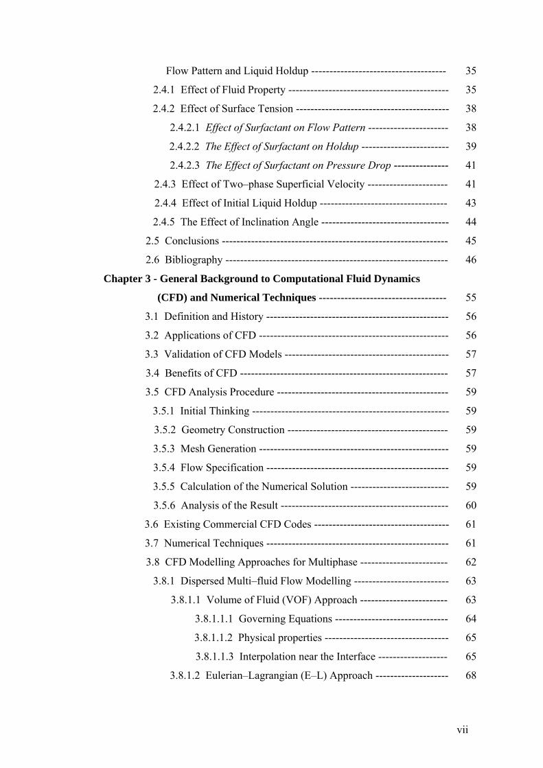
Table of Contents List of Publications ---------------------------------------------------------------------- i
Abstract ----------------------------------------------------------------------------------- ii
Acknowledgements --------------------------------------------------------------------- v
Table of Contents ------------------------------------------------------------------------ vi
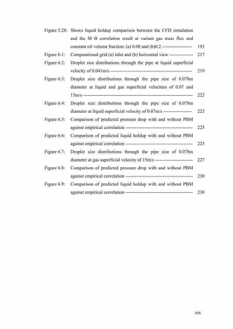
List of Figures ---------------------------------------------------------------------------- xiii
List of Tables ----------------------------------------------------------------------------- xx
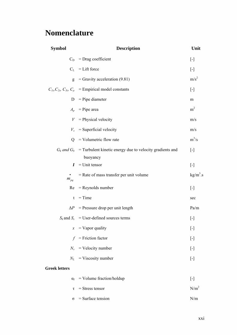
Nomenclature ---------------------------------------------------------------------------- xxi
Chapter 1 - Introduction -------------------------------------------------------------- 1
1.1 Motivation of this thesis ------------------------------------------------ 1
1.2 Objectives ----------------------------------------------------------------- 3
1.3 Contributions of the thesis ---------------------------------------------- 3
1.4 Thesis overview ---------------------------------------------------------- 4
1.5 Bibliography -------------------------------------------------------------- 8
Chapter 2 - Literature Review of Multiphase Flows in Pipelines ------------ 9
2.1 Hydrate Background ---------------------------------------------------- 10
2.2 Fundamental Concepts of Two–phase Gas Liquid Flows --------- 13
2.2.1 Definition of Basic Parameters ----------------------------------- 13
2.2.2 Multiphase Flow Regimes ----------------------------------------- 15
2.2.2.1 Classification of Gas–liquid Flow Patterns --------------- 16
2.2.3 Flow Patterns in Horizontal Pipes -------------------------------- 17
2.2.4 Flow Patterns in Vertical Pipes ----------------------------------- 19
2.2.5 Flow Pattern Maps -------------------------------------------------- 21
2.3 Liquid Holdup and Pressure Drop in Horizontal Pipelines -------- 24
2.3.1 Liquid Holdup Correlations of Adiabatic Two–phase Flow --- 24
2.3.2 Pressure Drop Correlations of Adiabatic Two–phase Flow --- 27
2.3.2.1 Correlation Based on Homogeneous Flow Model ------- 28
2.3.2.2 Correlations Based on the Multiplier Concept ------------ 29
2.3.2.3 Direct Empirical Models ------------------------------------- 31
2.3.2.4 Flow Pattern Specific Models ------------------------------- 33
2.4 Review of the Effect of Some Parameters on Pressure Drop,
vii
Flow Pattern and Liquid Holdup ------------------------------------- 35
2.4.1 Effect of Fluid Property -------------------------------------------- 35
2.4.2 Effect of Surface Tension ------------------------------------------ 38
2.4.2.1 Effect of Surfactant on Flow Pattern ---------------------- 38
2.4.2.2 The Effect of Surfactant on Holdup ------------------------ 39
2.4.2.3 The Effect of Surfactant on Pressure Drop --------------- 41
2.4.3 Effect of Two–phase Superficial Velocity ---------------------- 41
2.4.4 Effect of Initial Liquid Holdup ----------------------------------- 43
2.4.5 The Effect of Inclination Angle ----------------------------------- 44
2.5 Conclusions -------------------------------------------------------------- 45
2.6 Bibliography ------------------------------------------------------------- 46
Chapter 3 - General Background to Computational Fluid Dynamics
(CFD) and Numerical Techniques ----------------------------------- 55
3.1 Definition and History -------------------------------------------------- 56
3.2 Applications of CFD ---------------------------------------------------- 56
3.3 Validation of CFD Models --------------------------------------------- 57
3.4 Benefits of CFD --------------------------------------------------------- 57
3.5 CFD Analysis Procedure ----------------------------------------------- 59
3.5.1 Initial Thinking ------------------------------------------------------ 59
3.5.2 Geometry Construction -------------------------------------------- 59
3.5.3 Mesh Generation ---------------------------------------------------- 59
3.5.4 Flow Specification -------------------------------------------------- 59
3.5.5 Calculation of the Numerical Solution --------------------------- 59
3.5.6 Analysis of the Result ---------------------------------------------- 60
3.6 Existing Commercial CFD Codes ------------------------------------- 61
3.7 Numerical Techniques -------------------------------------------------- 61
3.8 CFD Modelling Approaches for Multiphase ------------------------ 62
3.8.1 Dispersed Multi–fluid Flow Modelling -------------------------- 63
3.8.1.1 Volume of Fluid (VOF) Approach ------------------------ 63
3.8.1.1.1 Governing Equations ------------------------------- 64
3.8.1.1.2 Physical properties ---------------------------------- 65
3.8.1.1.3 Interpolation near the Interface ------------------- 65
3.8.1.2 Eulerian–Lagrangian (E–L) Approach -------------------- 68
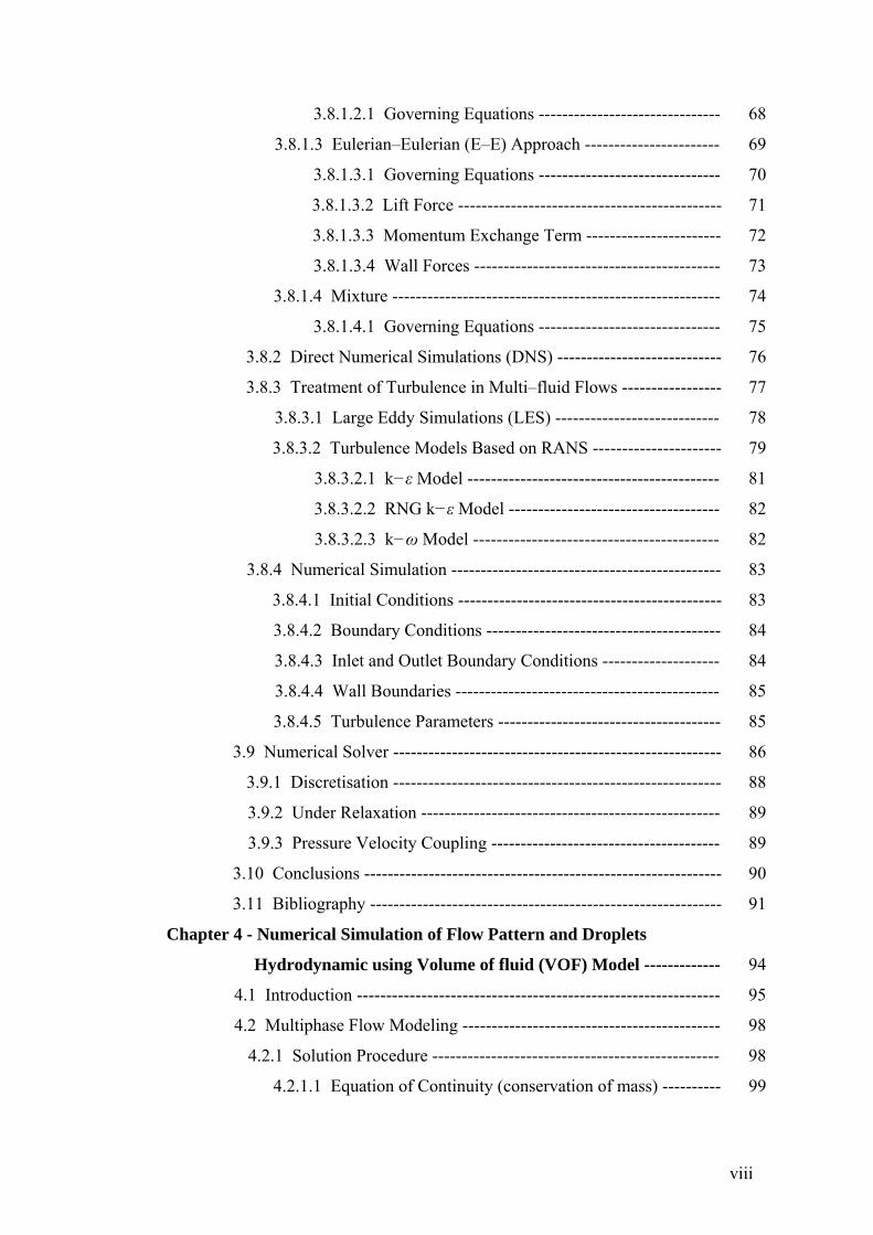
viii
3.8.1.2.1 Governing Equations ------------------------------- 68
3.8.1.3 Eulerian–Eulerian (E–E) Approach ----------------------- 69
3.8.1.3.1 Governing Equations ------------------------------- 70
3.8.1.3.2 Lift Force --------------------------------------------- 71
3.8.1.3.3 Momentum Exchange Term ----------------------- 72
3.8.1.3.4 Wall Forces ------------------------------------------ 73
3.8.1.4 Mixture -------------------------------------------------------- 74
3.8.1.4.1 Governing Equations ------------------------------- 75
3.8.2 Direct Numerical Simulations (DNS) ---------------------------- 76
3.8.3 Treatment of Turbulence in Multi–fluid Flows ----------------- 77
3.8.3.1 Large Eddy Simulations (LES) ---------------------------- 78
3.8.3.2 Turbulence Models Based on RANS ---------------------- 79
3.8.3.2.1 k−ε Model ------------------------------------------- 81
3.8.3.2.2 RNG k−ε Model ------------------------------------ 82
3.8.3.2.3 k−ω Model ------------------------------------------ 82
3.8.4 Numerical Simulation ---------------------------------------------- 83
3.8.4.1 Initial Conditions --------------------------------------------- 83
3.8.4.2 Boundary Conditions ---------------------------------------- 84
3.8.4.3 Inlet and Outlet Boundary Conditions -------------------- 84
3.8.4.4 Wall Boundaries --------------------------------------------- 85
3.8.4.5 Turbulence Parameters -------------------------------------- 85
3.9 Numerical Solver -------------------------------------------------------- 86
3.9.1 Discretisation -------------------------------------------------------- 88
3.9.2 Under Relaxation --------------------------------------------------- 89
3.9.3 Pressure Velocity Coupling --------------------------------------- 89
3.10 Conclusions ------------------------------------------------------------- 90
3.11 Bibliography ------------------------------------------------------------ 91
Chapter 4 - Numerical Simulation of Flow Pattern and Droplets
Hydrodynamic using Volume of fluid (VOF) Model ------------- 94
4.1 Introduction -------------------------------------------------------------- 95
4.2 Multiphase Flow Modeling -------------------------------------------- 98
4.2.1 Solution Procedure ------------------------------------------------- 98
4.2.1.1 Equation of Continuity (conservation of mass) ---------- 99
ix
4.2.1.2 Conservation of Momentum (Navier–Stokes equation) 99
4.2.1.3 The Volume Fraction Equation ---------------------------- 99
4.2.2 Turbulence Model -------------------------------------------------- 100
4.2.3 Physical Properties ------------------------------------------------- 100
4.2.4 Differencing Scheme/Solution Strategy and Convergence
Criterion -------------------------------------------------------------- 101
4.3 Description of the Pipeline Geometry and Operating Conditions 101
4.4 Air–water Simulation Results and Discussion ---------------------- 104
4.4.1 Low Liquid Patching with Different Restart Gas Velocities - 104
4.4.2 Medium Liquid Patching with Different Restart Gas
Velocities ----------------------------------------------------------- 106
4.4.3 High Liquid Patching with Different Restart Gas Velocities - 109
4.4.4 Compare the Flow Pattern Simulation with Flow Map for
1m Low Section Depth -------------------------------------------- 112
4.4.5 The Effect of Low Spot Depth ----------------------------------- 115
4.4.5.1 Low Liquid Patching with Different Restart Gas
Velocities ----------------------------------------------------- 115
4.4.5.2 Medium Liquid Patching with Different Restart Gas
Velocities ----------------------------------------------------- 119
4.4.5.3 High Liquid Patching with Different Restart Gas
Velocities ----------------------------------------------------- 123
4.4.5.4 Compare the Flow Pattern Simulation with Flow Map
for 2m Low Section Depth --------------------------------- 128
4.4.6 The Risk of Flow Pattern ----------------------------------------- 131
4.5 Air–oil Simulation Results and Discussion -------------------------- 133
4.5.1 Low Oil Patching with Different Restart Gas Velocities ------ 133
4.5.2 Medium Oil Patching with Different Restart Gas Velocities - 135
4.5.3 High Oil Patching with Different Restart Gas Velocities ----- 137
4.5.4 Liquid in the Low Section ----------------------------------------- 139
4.6 Comparison between 2-D and 3-D VOF Simulation for Water
with Constant Gas Restart Velocity ---------------------------------- 141
4.7 Conclusions -------------------------------------------------------------- 145
4.8 Bibliography ------------------------------------------------------------- 146
x
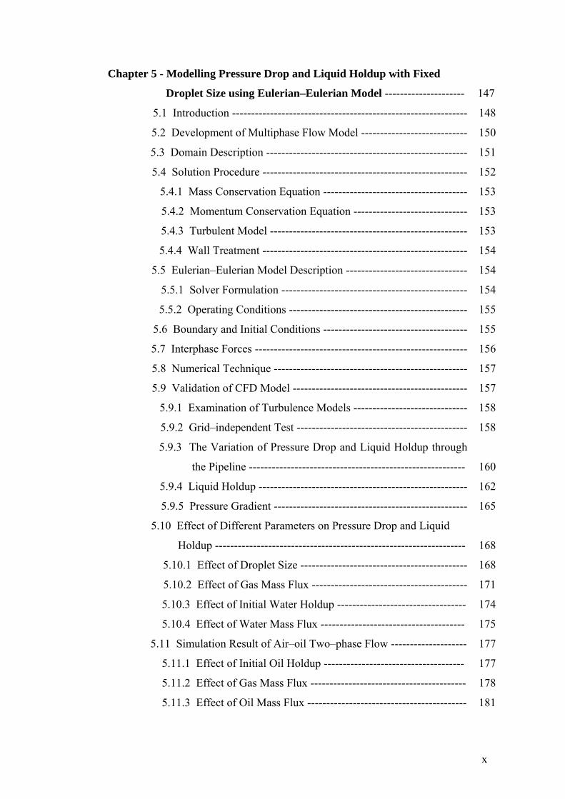
Chapter 5 - Modelling Pressure Drop and Liquid Holdup with Fixed
Droplet Size using Eulerian–Eulerian Model --------------------- 147
5.1 Introduction -------------------------------------------------------------- 148
5.2 Development of Multiphase Flow Model ---------------------------- 150
5.3 Domain Description ----------------------------------------------------- 151
5.4 Solution Procedure ------------------------------------------------------ 152
5.4.1 Mass Conservation Equation -------------------------------------- 153
5.4.2 Momentum Conservation Equation ------------------------------ 153
5.4.3 Turbulent Model ---------------------------------------------------- 153
5.4.4 Wall Treatment ------------------------------------------------------ 154
5.5 Eulerian–Eulerian Model Description -------------------------------- 154
5.5.1 Solver Formulation ------------------------------------------------- 154
5.5.2 Operating Conditions ----------------------------------------------- 155
5.6 Boundary and Initial Conditions -------------------------------------- 155
5.7 Interphase Forces -------------------------------------------------------- 156
5.8 Numerical Technique --------------------------------------------------- 157
5.9 Validation of CFD Model ---------------------------------------------- 157
5.9.1 Examination of Turbulence Models ------------------------------ 158
5.9.2 Grid–independent Test --------------------------------------------- 158
5.9.3 The Variation of Pressure Drop and Liquid Holdup through
the Pipeline --------------------------------------------------------- 160
5.9.4 Liquid Holdup ------------------------------------------------------- 162
5.9.5 Pressure Gradient --------------------------------------------------- 165
5.10 Effect of Different Parameters on Pressure Drop and Liquid
Holdup ------------------------------------------------------------------ 168
5.10.1 Effect of Droplet Size -------------------------------------------- 168
5.10.2 Effect of Gas Mass Flux ----------------------------------------- 171
5.10.3 Effect of Initial Water Holdup ---------------------------------- 174
5.10.4 Effect of Water Mass Flux -------------------------------------- 175
5.11 Simulation Result of Air–oil Two–phase Flow -------------------- 177
5.11.1 Effect of Initial Oil Holdup ------------------------------------- 177
5.11.2 Effect of Gas Mass Flux ----------------------------------------- 178
5.11.3 Effect of Oil Mass Flux ------------------------------------------ 181
xi
5.11.4 Comparison between Air–oil and Air–water Flow Results - 182
5.12 Comparison of CFD Result with An empirical Correlation ----- 183
5.12.1 Identified Flow Pattern ------------------------------------------ 184
5.12.2 Two–phase Pressure Drop -------------------------------------- 185
5.12.3 Liquid Holdup Correlation -------------------------------------- 186
5.12.4 Results and Discussion ------------------------------------------ 187
5.13 Conclusions ------------------------------------------------------------- 194
5.14 Bibliography ------------------------------------------------------------ 195
Chapter 6 - Prediction of System Parameters and Drop Size Distribution
using CFD and Population Balance Equation -------------------- 198
6.1 Introduction -------------------------------------------------------------- 199
6.2 Population Balance Equation ------------------------------------------ 201
6.3 Closure Models for Coalescence and Breakage --------------------- 204
6.3.1 Breakage Models --------------------------------------------------- 204
6.3.2 Coalescence Models ------------------------------------------------ 205
6.4 Numerical Techniques -------------------------------------------------- 206
6.4.1 The Discrete Method ----------------------------------------------- 206
6.4.2 The Standard Method of Moments ------------------------------- 208
6.4.3 The Quadrature Method of Moments ---------------------------- 209
6.5 Mathematical Modelling ----------------------------------------------- 210
6.5.1 Mass Conservation Equation -------------------------------------- 211
6.5.2 Momentum Transfer Equations ----------------------------------- 214
6.5.3 Turbulence Equations ---------------------------------------------- 215
6.6 Method of Solution ----------------------------------------------------- 216
6.7 Results and Discussion ------------------------------------------------- 218
6.7.1 Compare CFD–PBM Model with an Experimental Data ----- 218
6.7.2 Effect of Gas Superficial Velocity ------------------------------- 220
6.7.2.1 Droplet Size Distribution (DSD) --------------------------- 220
6.7.2.2 Pressure Drop and Liquid Holdup ------------------------- 223
6.7.3 Effect of Water Superficial Velocity ----------------------------- 226
6.7.3.1 Droplet Size Distribution (DSD) --------------------------- 226
6.7.3.2 Pressure Drop and Liquid Holdup ------------------------- 227
6.8 Conclusions -------------------------------------------------------------- 231
xii
6.9 Bibliography ------------------------------------------------------------- 232
Chapter 7 - Conclusions and Future Work --------------------------------------- 239
7.1 Summary and Conclusions --------------------------------------------- 239
7.1.1 Numerical Simulation of Two–phase Flow in Bend
Pipelines ------------------------------------------------------------- 240
7.1.2 Development of E–E Model for Two–phase Flow in
Horizontal Pipeline ------------------------------------------------- 241
7.1.3 Prediction of Droplet Size Distribution Using CFD-PBM
Model ---------------------------------------------------------------- 242
7.2 Recommendations for Future Work ---------------------------------- 242
7.2.1 Improvement to Droplet Hydrodynamic VOF model --------- 242
7.2.2 k–ε Model of Constant Droplet Size ----------------------------- 243
7.2.3 Improvements to CFD–PBM Model ----------------------------- 244
7.2.4 Recommendation on the Experimental Work ------------------- 244
7.3 Bibliography ------------------------------------------------------------- 244
xiii
List of Figures
Figure 1.1: The thesis structure ------------------------------------------------------ 7
Figure 2.1: Typical hydrate curve (Volk et al., 2010) ---------------------------- 11
Figure 2.2: Multiphase flow regimes (ANSYS FLUENT 12.1 Theory Guide,
2010) ---------------------------------------------------------------------- 16
Figure 2.3: Flow regimes in horizontal gas–liquid (Ali, 2009) ----------------- 19
Figure 2.4: Flow regimes in vertical gas–liquid upflow (Ali, 2009) ----------- 20
Figure 2.5: Mandhane (1974) flow pattern map for horizontal flow in a tube 22
Figure 2.6: Flow regimes map for vertical upflow showing Taitel et al.
(1980) and Mishima and Ishii (1984) transitions (Mishima and
Ishii, 1984) --------------------------------------------------------------- 23
Figure 2.7: Baker chart. (●) Operating conditions for the simulations of
water-air flow; (■) Operating conditions for the simulations of
gas oil liquid-vapor flow ----------------------------------------------- 23
Figure 3.1: A flow diagram of the CFD analysis procedure --------------------- 60
Figure 3.2: VOF interface reconstruction methods: (a) actual interface
shape, (b) interface reconstruction by means of the second-order
or PLIC method, and (c) interface reconstruction by means of
the first-order or SLIC method (Fluent 6.2 User’s Guide, 2005) - 66
Figure 3.3: Schematic representation of scales in turbulent flows (adapted
from Ferziger and Peric, 1995) ---------------------------------------- 78
Figure 3.4: A comparison of DNS, LES and RANS (Ranade, 2002) ---------- 80
Figure 3.5: FLUENT coupled solver ----------------------------------------------- 87
Figure 3.6: FLUENT segregated solver -------------------------------------------- 87
Figure 4.1: Pipeline Schematic ------------------------------------------------------ 103
Figure 4.2: Schematic of low point ------------------------------------------------- 103
Figure 4.3: Initial patched liquid phase: (a)20cm, (b)30cm, and (c)50cm ----- 103
Figure 4.4: Gas–liquid interface displacement from the low point for variant
superficial gas velocity: (a) 5m/s, and (b) 10m/s -------------------- 105
Figure 4.5: Sketch of water distribution with low and medium restart gas
velocity ------------------------------------------------------------------- 105
Figure 4.6: Sketch of water distributions with high restart gas velocity ------- 106
xiv
Figure 4.7: Shows the gas–liquid interface behaviour at low velocity 5m/s
and medium liquid patching ------------------------------------------- 107
Figure 4.8: Shows the effect of gas superficial velocity on medium liquid
patching 30 cm after 0.5 seconds, (a) 10m/s, (b) 15m/s, and (c)
20m/s ---------------------------------------------------------------------- 108
Figure 4.9: Shows the effect of various gas superficial velocities on the gas–
liquid interface in the horizontal section at medium liquid
patching, (a) 10m/s, (b) 15m/s, and (c) 20m/s ----------------------- 108
Figure 4.10: Shows the behaviour of the gas-liquid interface and water
contours in the low point section for high liquid patching 50cm
and low velocity 5m/s at different times ----------------------------- 110
Figure 4.11: Low gas superficial velocity (5m/s) and high liquid patching
behaviour in the horizontal section ----------------------------------- 110
Figure 4.12: Shows the gas-liquid interface behaviour at a low point section
for high liquid patching 50cm and at different gas velocities: (a)
10m/s, (b) 15m/s, and (c) 20m/s at 1 second of flowing time ----- 110
Figure 4.13: Medium and high restart gas velocities with high liquid patching
behaviour in the horizontal section ----------------------------------- 111
Figure 4.14: Comparison of flow pattern simulation with Baker flow map for
1m low section depth and low patched liquid at different gas
velocities ▲5m/s,■10m/s,●15m/s, and♦ 20m/s --------------------- 113
Figure 4.15: The remaining liquid at the low point at different gas superficial
velocity for a 1m low spot depth -------------------------------------- 114
Figure 4.16: A new low section geometry with 2m depth ------------------------ 115
Figure 4.17: Sketch for water fraction in the low point with time at low
velocity and liquid patched -------------------------------------------- 116
Figure 4.18: Water droplets contours in the low and horizontal section after 4
seconds -------------------------------------------------------------------- 116
Figure 4.19: Gas-liquid interface behaviour with time for superficial gas
velocity of 5m/s ---------------------------------------------------------- 116
Figure 4.20: Sketch for water fraction in the low point with time for different
gas velocities: (a) 10m/s and (b) 15m/s ------------------------------ 118
Figure 4.21: Gas-liquid interface behaviour with time for superficial gas
xv
velocity of 10m/s -------------------------------------------------------- 118
Figure 4.22: Gas–liquid interface behaviour with time for gas superficial
velocity of 15m/s -------------------------------------------------------- 118
Figure 4.23: The gas–liquid interface behaviour with time for gas superficial
velocity of 20m/s -------------------------------------------------------- 118
Figure 4.24: Sketch of water fraction behaviour at the lower section of pipe
for 5m/s at different flow times --------------------------------------- 120
Figure 4.25: Behaviour of gas–liquid interface in horizontal section at
medium liquid patching and 5m/s gas velocity ---------------------- 120
Figure 4.26: Sketch of two-phase behaviour at superficial gas velocity 10m/s
with different flow time ------------------------------------------------ 122
Figure 4.27: Water contours in the low and horizontal section for 15m/s at 0.5
seconds of flow time ---------------------------------------------------- 122
Figure 4.28: Sketch of gas-liquid interface for 15m/s at different flow times -- 122
Figure 4.29: Sketch of gas-liquid interface for 20m/s at different flow times -- 123
Figure 4.30: Water contours at low and horizontal sections at variant flow
time for 5m/s and high liquid patching ------------------------------- 125
Figure 4.31: Water contours at the low section at different flow times for
medium gas velocity and high liquid patching ---------------------- 126
Figure 4.32: Sketch of water contours and flow pattern at superficial gas
velocity of 10 m/s and high liquid patching ------------------------- 127
Figure 4.33: Sketch of water contours and flow pattern at superficial gas
velocity of 15m/s and high liquid patching -------------------------- 127
Figure 4.34: Sketch of water contours and flow pattern at superficial gas
velocity of 20m/s and high liquid patching -------------------------- 128
Figure 4.35: Compares flow pattern simulation with Baker flow map at 2m
low section depth and low patched liquid at different gas
velocities, ▲5m/s, ■10m/s, ●15m/s, and ♦20m/s ------------------ 129
Figure 4.36: Experimental results of water lift in the low section for the
second low spot ---------------------------------------------------------- 130
Figure 4.37: Flow pattern map indicates high and low risk areas of 1m low
section depth ------------------------------------------------------------- 132
Figure 4.38: Flow pattern map indicates high and low risk areas of 2m low
xvi
section depth ------------------------------------------------------------- 132
Figure 4.39: Sketch of oil fraction behaviour at the lower section of pipe for
5m/s at different flow times and low oil patching ------------------ 134
Figure 4.40: Sketch of air-oil interface for 10m/s at different flow times and
low oil patching ---------------------------------------------------------- 134
Figure 4.41: Sketch of air-oil interface for 15m/s at different flow times and
low oil patching ---------------------------------------------------------- 135
Figure 4.42: Sketch of air-oil interface for 20m/s at different flow times and
low oil patching ---------------------------------------------------------- 135
Figure 4.43: Sketch of air-oil interface at oil patching 0.3m for 5m/s at
different flow times ----------------------------------------------------- 136
Figure 4.44: Sketch of air-oil interface at 0.3m oil patching for 10m/s at
different flow times ----------------------------------------------------- 136
Figure 4.45: Sketch of air-oil interface at 0.3m oil patching for 10m/s at 8
second flow time -------------------------------------------------------- 136
Figure 4.46: Sketch of air-oil interface for 15m/s at different flow times at
medium liquid patching ------------------------------------------------ 137
Figure 4.47: Sketch of air-oil interface for 5m/s at different flow times and
high oil patching --------------------------------------------------------- 138
Figure 4.48: Sketch of air-oil interface for 10m/s at different flow times and
high oil patching --------------------------------------------------------- 138
Figure 4.49: Sketch of air-oil interface for 15m/s at different flow times and
high oil patching --------------------------------------------------------- 138
Figure 4.50: Sketch of air-oil interface for 20m/s at different flow times and
high oil patching --------------------------------------------------------- 138
Figure 4.51: Experimental results of remained oil in the low section for 1m
depth ---------------------------------------------------------------------- 140
Figure 4.52: Comparison between oil and water left in the low section for 1m
low spot depth at different liquid patching: (a)0.2 m, (b) 0.3 m,
and (c) 0.5 m ------------------------------------------------------------- 140
Figure 4.53: Typical computational domain grids representing the flow
domain discretisation for a bended pipe: (a) View of inlet
meshed pipeline (b) View of the meshed 3–D low section, and
xvii
(c) View of the meshed horizontal pipeline -------------------------- 142
Figure 4.54: Comparison between 2D and 3D simulation of air–water flow at
15 m/s at different water patching------------------------------------- 144
Figure 4.55: Comparison between 2D ■ and 3D ▲ simulation results of flow
patterns with the Baker chart at 15m/s and 0.3m water patching -- 145
Figure 5.1: (a) Inlet view of 3-D meshed model (b) View of the meshed 3-D
pipeline ------------------------------------------------------------------- 152
Figure 5.2: Shows the comparison of pressure gradient between the
experimental data and different turbulence k–ε models ------------ 159
Figure 5.3: Shows the comparison of liquid holdup between the experiment–
al data and different turbulence k–ε models ------------------------- 160
Figure 5.4: Shows the liquid holdup across the pipeline ------------------------- 161
Figure 5.5: Shows the pressure drop across the pipeline ------------------------- 161
Figure 5.6: Shows liquid holdup contours at outlet for constant superficial
water velocity 0.035 m/s and variant superficial gas velocity (a)
15 m/s, (b) 20 m/s, and (c) 25 m/s ------------------------------------ 162
Figure 5.7: Region of air–water flow data plotted on (Taitel and Dukler,
1976) flow pattern map ------------------------------------------------- 163
Figure 5.8: Shows liquid holdup at different superficial gas velocity and
constant liquid superficial velocity ----------------------------------- 164
Figure 5.9: Shows liquid holdup at different superficial gas velocity and
constant superficial liquid velocity ----------------------------------- 164
Figure 5.10: Shows CFD comparison of pressure gradient with an
experimental data and (a) the Hart et al. model and (b) the Chen
et al. model ---------------------------------------------------------------
167
Figure 5.11: Shows CFD comparison of pressure gradient with an
experimental data -------------------------------------------------------- 167
Figure 5.12: Demonstrates the effect of water superficial velocity on pressure
gradient at high gas superficial velocity ------------------------------ 169
Figure 5.13: Demonstrates the effect of water superficial velocity on liquid
holdup at high gas superficial velocity ------------------------------- 170
Figure 5.14: Shows liquid holdup contours at outlet for constant superficial
gas velocity (25m/s) and variant droplet size: (a) 100μm, and (b)
xviii
300μm --------------------------------------------------------------------- 170
Figure 5.15: Shows CFD pressure drop versus different gas mass flux at
constant water fraction -------------------------------------------------- 171
Figure 5.16: Shows CFD water holdup versus different gas superficial
velocity at different initial water fractions (a) 0.04, (b) 0.08, (c)
0.12, (d) 0.16, and (e) 0.2 ---------------------------------------------- 173
Figure 5.17: Shows CFD pressure drop versus different initial water fraction
at constant total mass flux ---------------------------------------------- 174
Figure 5.18: Shows the effect of water mass flux on pressure drop at constant
water fraction and gas mass flux -------------------------------------- 176
Figure 5.19: Shows the effect of water mass flux on liquid holdup at constant
water fraction and gas mass flux -------------------------------------- 176
Figure 5.20: Shows the effect of oil volume fraction on pressure drop at
constant two–phase flux ------------------------------------------------ 178
Figure 5.21: Demonstrates the effect of gas mass flux on pressure drop at a
constant input oil volume fraction: (a) 0.04, (b) 0.08, (c) 0.12,
(d) 0.16, and (e) 0.2 ----------------------------------------------------- 179
Figure 5.22: Demonstrates the effect of gas mass flux on liquid holdup at a
constant input oil volume fraction: (a) 0.04, (b) 0.08, (c) 0.12,
(d) 0.16, and (e) 0.2 ----------------------------------------------------- 180
Figure 5.23: Shows the effect of oil mass flux on pressure drop at constant
gas mass flux and liquid volume fraction ---------------------------- 181
Figure 5.24: Shows the effect of oil mass flux on liquid holdup at constant
gas mass flux and liquid volume fraction ---------------------------- 182
Figure 5.25: Shows comparison between the CFD and the B–B correlation
pressure drop of air–water at different gas mass flux and
constant liquid volume fraction (a) 0.08 and (b) 0.2 ---------------- 189
Figure 5.26: Shows comparison between the CFD and the B–B correlation
pressure drop of air–oil at different gas mass flux and constant
liquid volume fraction (a) 0.08 and (b) 0.2 -------------------------- 190
Figure 5.27: Shows liquid holdup comparison between the CFD simulation
and the M–B correlation results at variant gas mass flux and
constant water volume fraction: (a)0.08 and (b)0.2 ----------------- 192
xix
Figure 5.28: Shows liquid holdup comparison between the CFD simulation
and the M–B correlation result at variant gas mass flux and
constant oil volume fraction: (a) 0.08 and (b)0.2 ------------------- 193
Figure 6.1: Computational grid (a) inlet and (b) horizontal view --------------- 217
Figure 6.2: Droplet size distributions through the pipe at liquid superficial
velocity of 0.041m/s ---------------------------------------------------- 219
Figure 6.3: Droplet size distributions through the pipe size of 0.078m
diameter at liquid and gas superficial velocities of 0.07 and
15m/s ---------------------------------------------------------------------- 222
Figure 6.4: Droplet size distributions through the pipe size of 0.078m
diameter at liquid superficial velocity of 0.07m/s ------------------ 222
Figure 6.5: Comparison of predicted pressure drop with and without PBM
against empirical correlation ------------------------------------------- 225
Figure 6.6: Comparison of predicted liquid holdup with and without PBM
against empirical correlation ------------------------------------------- 225
Figure 6.7: Droplet size distributions through the pipe size of 0.078m
diameter at gas superficial velocity of 15m/s ------------------------ 227
Figure 6.8: Comparison of predicted pressure drop with and without PBM
against empirical correlation ------------------------------------------- 230
Figure 6.9: Comparison of predicted liquid holdup with and without PBM
against empirical correlation ------------------------------------------- 230
xx
List of Tables
Table:2.1 Most Common of Liquid Holdup Correlations ------------------------ 25
Table:2.2 Commonly Used Correlations for Friction Factor Calculation of
Circular Cross–section Pipes --------------------------------------------- 28
Table:2.3 Existing Correlations for Homogeneous Model for Two–phase
Pressure Drop --------------------------------------------------------------- 29
Table:2.4 Existing Correlations for Two–phase Pressure Drop Based on the
Multiplier Concept in Horizontal Pipeline ----------------------------- 30
Table:2.5 Existing Correlations for Flow Pattern Specific Two–phase
Pressure Drop for Horizontal, Vertical and Inclined Pipeline ------- 34
Table:4.1 Physical Properties of Water and Air (T =298 K and P =101.325
KPa) ------------------------------------------------------------------------- 104
Table:4.2 Flow Patterns for Low Liquid Patching (0.2m) at Different Restart
Gas Superficial Velocities ------------------------------------------------ 113
Table:4.3 Flow Patterns for Low Liquid Loading at Different Restart Gas
Superficial Velocities for 2m Low Section Depth --------------------- 128
Table:5.1 Effect of Grid Size on Pressure Drop Using RNG k-ε Model at a
Constant Superficial Water Velocity 0.025m/s ------------------------ 159
xxi
Nomenclature Symbol Description Unit
CD = Drag coefficient [-]
CL = Lift force [-]
g = Gravity acceleration (9.81) m/s2
C1ε,C2ε, C3ε, Cμ = Empirical model constants [-]
D = Pipe diameter m
Ap = Pipe area m2
V = Physical velocity m/s
Vs = Superficial velocity m/s
Q = Volumetric flow rate m3/s
Gk and Gb = Turbulent kinetic energy due to velocity gradients and
buoyancy
[-]
I = Unit tensor [-]
pqm = Rate of mass transfer per unit volume kg/m3.s
Re = Reynolds number [-]
t = Time sec
ΔP = Pressure drop per unit length Pa/m
Sk and Sε = User-defined sources terms [-]
x = Vapor quality [-]
f = Friction factor [-]
Nv = Velocity number [-]
NL = Viscosity number [-]
Greek letters
αl = Volume fraction/holdup [-]
τ = Stress tensor N/m2
σ = Surface tension N/m
xxii
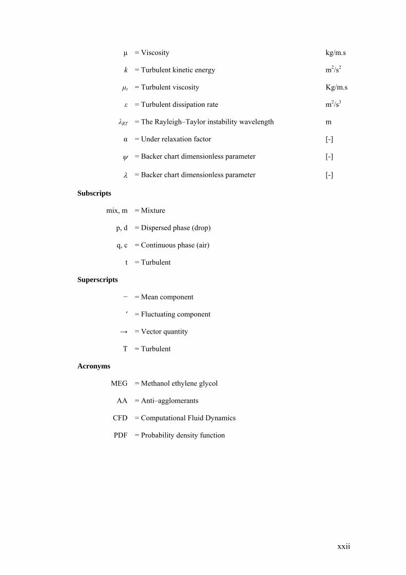
μ = Viscosity kg/m.s
k = Turbulent kinetic energy m2/s2
μt = Turbulent viscosity Kg/m.s
ε = Turbulent dissipation rate m2/s3
λRT = The Rayleigh–Taylor instability wavelength m
α = Under relaxation factor [-]
= Backer chart dimensionless parameter [-]
= Backer chart dimensionless parameter [-]
Subscripts
mix, m = Mixture
p, d = Dispersed phase (drop)
q, c = Continuous phase (air)
t = Turbulent
Superscripts
− = Mean component
′ = Fluctuating component
→ = Vector quantity
T = Turbulent
Acronyms
MEG = Methanol ethylene glycol
AA = Anti–agglomerants
CFD = Computational Fluid Dynamics
PDF = Probability density function
Chapter 1. Introduction _______________________________________________________________________________________________________
1.1 Motivation for this thesisaccumulates at the bottom.
Two–phase flow is a very common occurrence in many petroleum subsea systems
where crude oil and gas is transported from offshore wells. In these applications, the
two-phase flow can mix and form different flow regimes and patterns. The flow
pattern is a very important feature of two–phase flow where the interface can be
distributed in several shapes such as wavy, dispersed, and annular flow. During the
hydrocarbon transportation process, the variation of phase temperature and pressure
throughout the pipeline can cause the formation of a small quantity of liquid (water),
to accumulate in the lowest section of the pipeline due to gravity as the pipeline
profile is usually curved following the sea bed structure.
In two–phase flow water introduces new challenges related to flow assurance such as
wax formation, scale deposits, and gas hydrate. Attention has been given to this
phenomenon, which takes place in curved sections of the pipeline where the liquid is
trapped. The critical velocity that is required at restart operation to sweep the liquid
from the lower section can create different flow patterns. These could be undesirable
for subsea system conditions. The understanding of flow behaviour is important for
safety operation, control and design.
Design parameters such as pressure drop in a single–phase flow in conduits can be
modelled easily. However the existence of a second phase such as water can lead to a
significant increase in the pressure drop, and creates difficult challenges in the
understanding and modelling of the flow system.
The flow hydrodynamics and mechanisms change significantly from one flow pattern
to another. For instance, it has been illustrated (Cheremisinoff, 1986) that for similar
flow conditions, slug flow and wavy flow may result in a difference in the pressure
drop of a factor of two. In recent decades, researchers have given attention to two–
phase flow because of its importance in the oil and gas industry, where the three most
important hydrodynamic characteristics of two–phase flow in pipes are the flow
pattern, the two–phase holdup, and the pressure drop. In order to predict the holdup
Chapter 1. Introduction ___________________________________________________________________________________
2
and pressure drop precisely, it is necessary to know the flow pattern under specific
flow conditions. Different flow maps published over recent decades can be utilized to
recognize the flow pattern. The most widely used flow pattern maps for predicting the
two–phase flow regimes for adiabatic flow in horizontal pipelines are those of Baker
(1954), Taitel and Dukler (1976), and Barnea and Taitel (1986).
A good understanding and an accurate description of fluid flow and drop size
distribution in horizontal pipelines is necessary for the modelling of pressure drop,
however accurate modelling of pressure drop and liquid holdup is complicated due to
the complexity of flow configurations generated by the two–phase velocity. Over the
last ten years, Computational Fluid Dynamics (CFD) has become an industrial
simulation tool for an engineering system investigation which includes fluid flow,
design, analysis, and performance determination. This improvement has been made
due to the easy accessibility of robust in–house systems and the enormous increase in
computer memory capacity and speed, resulting in a reduction in the costs of
simulation compared to experimental work. With the CFD tool it is possible to get a
detailed view of the flow, and specific data for liquid holdup and pressure drop
behavior in horizontal pipelines.
It is also possible to model two–phase pressure drop and liquid holdup, accounting for
a higher intensity explanation of the physical processes between the two–phase, and
the coalescence and break–up phenomena of droplets influencing the dynamics of
both phases, as well as the mass transfer between them. For this reason, the
understanding of the droplet size distribution or of the droplet population evolution is
of paramount significance for an accurate prediction of pressure drop and liquid
holdup. Such a higher order physical model should integrate an Eulerian–Eulerian
multiphase model and the Droplet Population Balance Equation (DPBE), which takes
into account the breakage and aggregation of the droplet, which affects the final
droplet size distribution and other system parameters.
Chapter 1. Introduction ___________________________________________________________________________________
3
1.2 Objectives
The aim of this research is to study two–phase flow behaviour in bend pipelines and
to investigate the pressure drop and liquid holdup of two fluids in two areas: flow of
gas–water and two–phase gas–oil flow. This research does not involve new numerical
development codes; rather it utilizes the suitably existing CFD models with compiled
user defined function (UDF) for the drag coefficient in order to conduct extensive
simulations. These are validated using experimental data from the open literature or
empirical correlations. The objectives of the study are:
1. To study the effect of restart gas superficial velocity, liquid loading and
low section depth on flow behaviour.
2. To predict the flow pattern in curved pipelines and compare this with one
of the flow pattern maps, and to develop a flow map for subsea systems
based on the results obtained.
3. To set up an Eulerian–Eulerian model for predicting pressure drop and
liquid holdup at fixed droplet size, and to compare this with experimental
data and/or correlations.
4. To investigate the effects of droplet size, initial liquid holdup, and mass
flux on the pressure drop and liquid holdup.
5. To evaluate the performance of CFD models with the population balance
for predicting the pressure drop, liquid holdup and droplet size
distribution.
1.3 Contributions of the Thesis
The current effort made contributions toward all of the above objectives, namely:
• It contributes to an understanding of the flow behaviour of two–phase in bend
pipes at different restart gas velocities and initial liquid patching.
Chapter 1. Introduction ___________________________________________________________________________________
4
• It identifies the risk of hydrate formation based on the generated flow pattern
map. This will assist the operators to understand the operating conditions
which have a high risk of hydrate formation.
• It develops a two–phase flow model for modelling the pressure drop and liquid
holdup by implementing a new drag coefficient. The Ishii–Chawla (1997) drag
coefficient for gas–liquid flow has been implemented using a User Defined
Function (UDF) and coupled with Eulerian–Eulerian multiphase flow.
• The developed CFD model predicts the pressure drop and liquid holdup data
more accurately than the existing models such as Hart et al. (1989) and Chen
et al. (1997) compared to the experimental data of Badie et al. (2000).
• The developed CFD model can be used to investigate the effect of various
parameters on the pressure drop and liquid holdup in horizontal pipes with low
liquid loading.
• The introduced population balance model combined with the CFD model
develops the gas–liquid two–phase flow model prediction behaviour in terms
of drop size distribution, pressure drop, and liquid holdup.
1.4 Thesis Overview
With the objectives provided by the current chapter, the remainder of this thesis
provides a comprehensive development of research performed in the above areas. A
brief description of the chapters is given as follows:
Chapter 2 commences with a literature review of the gas hydrate formation focusing
on critical places where it can occur, such as the lower section of the pipe. It also
provides the mechanism of an agglomeration process, and the way to avoid and
dissociate hydrates using inhibitor injection, followed by real case studies.
Furthermore, it also includes a literature review of two–phase flow in horizontal and
Chapter 1. Introduction ___________________________________________________________________________________
5
vertical conduits in terms of flow maps, flow patterns, and experimental work on
pressure drop and liquid holdup.
A summary of the published correlations on liquid holdup and pressure drop is
presented. The pressure drop correlations are classified based on a homogenous
model, a two–phase friction multiplier model, direct empirical models, and flow
regime specific models. In addition, a review of published experimental work on the
effects of various parameters on the pressure drop, liquid holdup, and flow pattern in
different pipe inclination angles are given.
Chapter 3 provides a general background to CFD including its applications,
advantages, CFD analysis procedure, and methodology. It also outlines the numerical
techniques used in this work.
Chapter 4 presents a brief review of published experimental work on gas hydrates in
subsea systems, in which the key issues were identified. It also presents the Volume
of Fluid (VOF) multiphase flow model for two and three–dimensional simulations
and unsteady state numerical model of gas–liquid two–phase counter current
horizontal flow regimes. Different restart gas velocities with initial liquid patching at
the low section have been investigated numerically to find out the flow behaviour and
to recognize the risk of hydrate formation. The simulation results were compared
experimentally to those found in the open literature data (taken from the Baker (1954)
chart).
Chapter 5 commences with published computational studies on two–phase flow
pressure drop and liquid holdup in a horizontal pipeline, and defines the modelling
problem. Controlling parameters (i.e. gas and liquid superficial velocity, and initial
liquid holdup) and model assumptions were stated. Three turbulence models based on
an Eulerian description were evaluated. The modelling adopts the RNG k–ε
turbulence model in conjunction with the enhanced wall treatment method. The
Eulerian–Eulerian two–phase flow model was developed by implementing the Ishii–
Chawla drag coefficient using the User Defined Function (UDF) in which C+ program
Chapter 1. Introduction ___________________________________________________________________________________
6
is used for writing the UDF. The implemented UDF was used for modelling the
pressure drop and liquid holdup. Various simulation case studies were conducted in
order to demonstrate the applicability of the developed two–phase model.
The numerical results from the developed CFD model were compared with the
existing models and with experimental data in order to test the accuracy and discuss
the performance of the model and its limitations. Furthermore, the sensitivity analysis
of different variables in the model was performed in order to test and find out the
behaviour of system pressure drop and liquid holdup.
Chapter 6 introduces the Population Balance Equation for droplets that can break and
aggregate due to droplet–droplet and droplet–fluid interactions. Under these
circumstances a fixed droplet size model might not be suitable for predicting the
correct thermo–fluid dynamics of the gas–liquid two–phase flow system. Many
researchers have tried to solve the population balance equation in which several
numerical methods are demonstrated. Most emphasis is given to studying the effect of
different system factors on the particle size distribution, pressure drop and liquid
holdup of two–phase flow in a horizontal conduit.
Finally, Chapter 7 summarizes the main outcomes from this work and presents
recommendations for further work.
Figure (1.1) gives a diagrammatic sketch of the thesis outline.
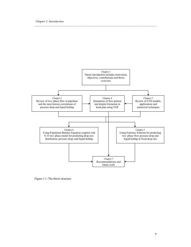
Chapter 1. Introduction ___________________________________________________________________________________
7
Figure 1.1: The thesis structure
Chapter 1
Thesis introduction includes motivation,
objectives, contributions and thesis
overview
Chapter 2
Review of two–phase flow in pipelines
and the most known correlations of
pressure drop and liquid holdup
Chapter 3
Review of CFD models,
applications and
numerical techniques
Chapter 4
Simulation of flow pattern
and droplet formation in
bend pipe using VOF
Chapter 5
Using Eulerian–Eulerian for predicting
two–phase flow pressure drop and
liquid holdup at fixed drop size
Chapter 6
Using Population Balance Equation coupled with
E–E two–phase model for predicting drop size
distribution, pressure drop, and liquid holdup
Chapter 7
Recommendations and future work
Chapter 1. Introduction ___________________________________________________________________________________
8
1.5 Bibliography
Badie, S., C. P. Hale, C. J. Lawrence and G. F. Hewitt (2000). Pressure gradient and
holdup in horizontal two-Phase gas-liquid flows with low liquid loading.
International Journal of Multiphase Flow, 26, 1525-1543.
Baker, O. (1954). Design pipelines for simultaneous flow of oil and gas. Oil and Gas
Journal, 53, 26.
Barnea, D. and Y. Taitel (1986). Flow pattern transition in two-phase gas-liquid
flows. Encyclopedia of Fluid Mechanics, 3, 403-474.
Chen, X. T., X. D. Cai and J. P. Brill (1997). Gas–Liquid stratified-wavy flow in
horizontal pipelines. Journal of Energy Resources Technology, 119(4), 209-
216.
Cheremisinoff N. P. (1986). Properties and concepts of single fluid flows.
Encyclopaedia of fluid mechanics, V, 1, flow phenomena and measurement,
285-351
Hart, J., P. J. Hamersma and J. M. H. Fortuin (1989). Correlations predicting
frictional pressure drop and liquid holdup during horizontal gas-liquid pipe
flow with a small liquid holdup. International Journal of Multiphase Flow,
15(5), 947-964.
Ishii M. and T. C. Chawla (1979). Local drag laws in dispersed two-phase flow,
NUREG/CR-1230, ANL-79-105.
Taitel, Y. and A. E. Dukler (1976). A model for predicting flow regime transitions in
horizontal and near horizontal gas- liquid flow. AIChE Journal, 22(1), 47-55.
“Every reasonable effort has been made to acknowledge the owners of copyright
material. I would be pleased to hear from any copyright owner who has been omitted
or incorrectly acknowledged.”
Chapter 2 Literature Review of Multiphase Flows in
Pipelines
This chapter will cover some topics which are relevant to subsea system and hydrate.
The first section describes the hydrate, for example: what is a hydrate? How does it
form? How could it be prevented?
Hydrate formation is closely related to offshore operations and a review of two–phase
flow in subsea systems particularly focused on pipelines will follow. Flow behavior in
horizontal pipes will be reviewed, including the flow pattern and flow map. Then,
operating factors that affect the pressure drop and liquid holdup will be covered with
some case studies.
Chapter 2. Literature Review of Multiphase Flows in Pipelines _______________________________________________________________________________________________________
10
2.1 Hydrate Background
In general, oil and gas offshore production can be very expensive, especially in deep
water due to the difficulty of access to crude oil reservoirs and because of the
problems of flow assurance due to low temperatures encountered at the seabed. Since
the production of oil and gas has moved to offshore, the flow assurance practice has
become very important to finding out the cost effectiveness and technical feasibility
of a deep water development. There are some flow assurance difficulties that are
common which take place in multiphase flows in pipelines. These include hydrate
formation which occurs because of the water and gas reaction. This leads to the
formation of solid particles that can cause pipe plugging; wax deposition on the pipe
wall which can reduce the diameter of the pipe until the flow is decreased and as a
result it can also plug the pipe and kill the well; asphaltene deposition; scale
precipitation; corrosion problems; and severe slugging. In order to reduce these
problems which have both practical and economic implications, the water has to be
removed.
Hydrates are usually crystalline particles created from the reaction between water and
a hydrocarbon gas at low pressure and high temperature, conditions which are most
likely to be found in deep water. Three hydrate crystal structures have been
recognized, these are structure I, II and H. Structures I and II are the most common
hydrate crystal structures and are composed mostly of light hydrocarbons, including
methane, ethane, propane, and isobutane, as well as many nonpolar molecules (such
as carbon dioxide, nitrogen, argon, krypton, and xenon). Larger molecules (e.g., 2,2-
dimethylbutane, cycloheptane) can also stabilize the hydrate structure (fitting into the
51268 cavities of structure H) in the presence of a smaller guest molecule (e.g.,
methane, xenon) that occupies the small cavities (435663 and 512) (Amadeu et al.,
2009).
The formation of these structures is based on gas molecules trapped by water
molecules. The pressure and temperature (P–T) hydrate curve diagram can be created
by using one of the software programs such as PVTSim or Multiflash based on the
fluids composition. Figure (2.1) shows that hydrate can form in the area to the left
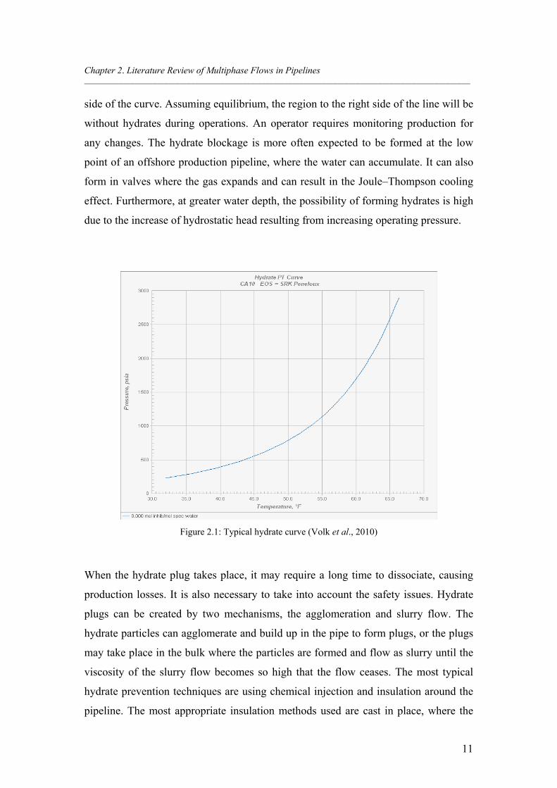
Chapter 2. Literature Review of Multiphase Flows in Pipelines _______________________________________________________________________________________________________
11
side of the curve. Assuming equilibrium, the region to the right side of the line will be
without hydrates during operations. An operator requires monitoring production for
any changes. The hydrate blockage is more often expected to be formed at the low
point of an offshore production pipeline, where the water can accumulate. It can also
form in valves where the gas expands and can result in the Joule–Thompson cooling
effect. Furthermore, at greater water depth, the possibility of forming hydrates is high
due to the increase of hydrostatic head resulting from increasing operating pressure.
Figure 2.1: Typical hydrate curve (Volk et al., 2010)
When the hydrate plug takes place, it may require a long time to dissociate, causing
production losses. It is also necessary to take into account the safety issues. Hydrate
plugs can be created by two mechanisms, the agglomeration and slurry flow. The
hydrate particles can agglomerate and build up in the pipe to form plugs, or the plugs
may take place in the bulk where the particles are formed and flow as slurry until the
viscosity of the slurry flow becomes so high that the flow ceases. The most typical
hydrate prevention techniques are using chemical injection and insulation around the
pipeline. The most appropriate insulation methods used are cast in place, where the
Chapter 2. Literature Review of Multiphase Flows in Pipelines _______________________________________________________________________________________________________
12
insulation layers are placed around the pipe, and pipe in pipe, where the production
line is put inside another pipe and the space (annulus) between the pipes is filled with
insulating material. This method of pipe–in–pipe is usually more costly.
Throughout the production of steady state, the insulation around the pipe may
maintain the system away from the hydrate region, but when the shutdown takes place
the fluids temperature in the pipeline may drop down to the sea temperature (typically
around 5oC). If the period of the shutdown does not go beyond the time of minimum
cool down, no action is required before the restart production. On the other hand, if
the time is longer, fluid conditions are more likely to occur inside the hydrate zone
and mitigation procedures are taken immediately. In this case, the chemical injection
technique is sufficient to avoid or delay hydrate formation, but is also expensive.
There are two common types of hydrate inhibitors; these are low dosage hydrate
inhibitors and thermodynamic inhibitors. The addition of thermodynamic inhibitors
such as methanol ethylene glycol (MEG) results in shifting the hydrate curve to a
lower temperature, making the hydrate zone smaller. The other type of inhibitor (low
dosage hydrate) is categorized as kinetic inhibitors, which cause a delay of the process
of hydrate nucleation, growth and anti–agglomerants (AA) that allow hydrates to form
without agglomeration. Other approaches that are available to prevent hydrate plugs
are water removal, operating at low pressure, and active heating, but they are either
too expensive or not practical. Even with these prevention methods, occasionally a
hydrate plug still forms and the most practical solution to dissociate is to inject
methanol. Other possible solutions used to dissociate hydrate plugs are heating the line,
and two sided depressurization. In all situations, the dissociation must be made in a safe
manner.
Many case studies of hydrate plug dissociation in subsea systems are presented by
Sloan (2000), where the equipment was completely destroyed and lives were lost
during an attempt to remove the hydrate plug. In 1991 there was an incident where
operators were trying to remove the plug in a sour–gas flow pipeline. During the
operation of plug dissociation, the pipeline was ruptured because of the effect of the
Chapter 2. Literature Review of Multiphase Flows in Pipelines _______________________________________________________________________________________________________
13
hydrate plug, resulting in loss of life. In another incident in the same year the method
of two sided depressurization to remove the plug was utilized, but the multiple plugs
could have resulted in the failure of a 3 inch Schedule 40 pipeline. Although
engineers have attempted to design a hydrate free well, they still occur, sometimes
leading to losses of life and equipment.
2.2 Fundamental Concepts of Two–phase Gas Liquid Flows
This section demonstrates some of the basic concepts and variables that are related to
two–phase flow in pipelines. The flow behaviour encountered in vertical and
horizontal pipelines is described, based on their characteristics. The flow pattern maps
which describe the flow pattern information are also introduced.
2.2.1 Definition of Basic Parameters The two–phase flow can be identified at the inlet boundary in different ways, as
mentioned in section (3.7.3.2.1). One of them is the inlet velocity, which is also called
the physical velocity. The physical velocity of each phase can be obtained based on
the superficial velocity and the in situ volume fraction of each phase, as follows:
L
SLL
VV
and
G
SGG
VV
(2.1)
Where VL and VG are the physical (or called true average) velocities of liquid and gas
phases respectively, and are larger than the superficial velocities.
The superficial velocities of the liquid and gas phases (VSL and VSG) are expressed as
the volumetric flow rate for the phase divided by the cross sectional area of the pipe
and can be written as:
p
LSL A
QV and
p
GSG A
QV (2.2)
Chapter 2. Literature Review of Multiphase Flows in Pipelines _______________________________________________________________________________________________________
14
Where QL and QG are the liquid and gas volumetric flow rate respectively and Ap
refers to the pipe cross sectional area.
Mass flux is also another method that can be used to specify the inlet boundary, by
dividing the mass flow rate by the inlet zone area. It is recommended that this is
utilized in situations where it is needed to study the effect of particular parameters
(i.e. volume fraction, flow rate) where a uniform mass flux is applied over the
domain. It is calculated by using the following form:
pflux A
mM
(2.3)
When using the mixture model, it is necessary to use the mixture properties.
Therefore, the mixture velocity is obtained by the sum of the gas and liquid
superficial velocities:
GLSGSLm xVVxVVV )1( (2.4)
In the homogeneous fluid flow, the two–phase volume fraction is calculated via
dividing the volumetric flow rate of a particular phase by the total volumetric flow
rate, where the sum of volume fractions of the liquid and gas phases (αl and αg) is
equal to unity. It can be obtained as:
m
SL
GL
Ll V
V
Q
(2.5)
m
SG
GL
Gg V
V
Q
(2.6)
The typical feature of two–phase flow is that two phases are distinguished by
viscosity and density, and flow counter or co–current. Typically the velocity of the
Chapter 2. Literature Review of Multiphase Flows in Pipelines _______________________________________________________________________________________________________
15
phase that is less dense and/or less viscous tends to flow fast in horizontal and uphill
flows. Moreover, in this type of pipe inclination, the gas phase travels much faster
than the liquid phase except in the situation of downward flow. Therefore, the
difference in the in situ average velocities between the two phases results in a very
important phenomenon , which is the “slip” of one phase relative to the other, or the
“holdup” of one phase relative to the other (Govier and Aziz, 1972). This leads to
different volume fractions between in situ and input. Although “holdup” can be
described as the fraction of the pipe volume occupied by a specified phase, holdup is
usually referred to as the in situ liquid volume fraction, while the term “void fraction”
is typically utilized for the in situ gas volume fraction.
The liquid holdup and gas void fraction are obtained by dividing the cross sectional
area that is occupied by one of the phases by the total area. The liquid holdup and gas
volume fractions are defined as:
p
LL A
A and
p
GG A
A (2.7)
Where AL and AG are the cross sectional areas, occupied by liquid and gas,
respectively.
Furthermore, the fluid property of each phase, such as density, viscosity and
interfacial tension, and the pipe internal diameter and inclination angle also have an
impact on the performance of the system. In the following sections the flow patterns
in horizontal and vertical pipes, and the pressure drop as well as the liquid holdup in
horizontal pipelines are reviewed and discussed.
2.2.2 Multiphase Flow Regimes
The flow regime typically is defined by a classification of flow pattern or a
description of the morphological arrangement of the phases (Wallis, 1969). In
addition, multiphase flow regimes are categorized into four classes, which are gas-
solid flows, liquid-solid flows, gas-liquid or liquid-liquid flows and three phases flow
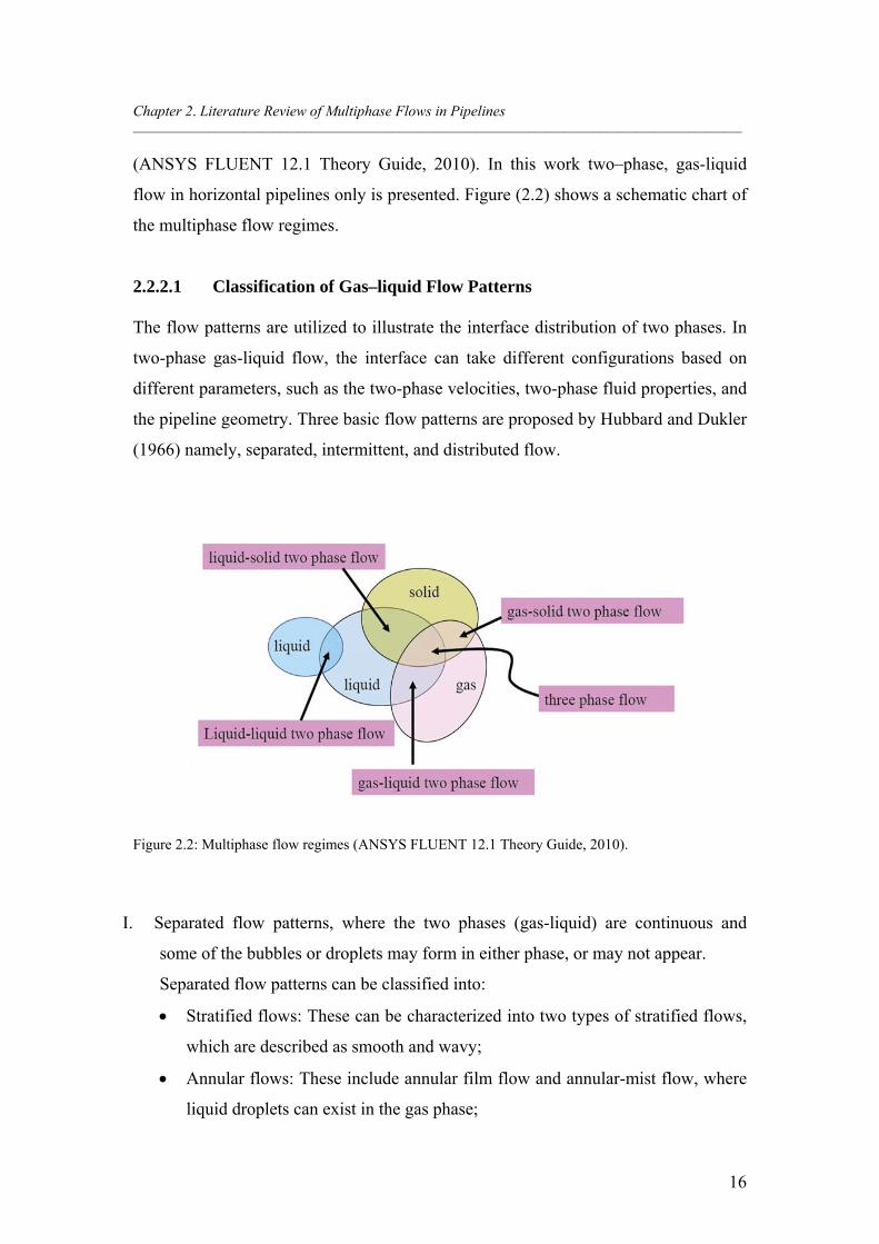
Chapter 2. Literature Review of Multiphase Flows in Pipelines _______________________________________________________________________________________________________
16
(ANSYS FLUENT 12.1 Theory Guide, 2010). In this work two–phase, gas-liquid
flow in horizontal pipelines only is presented. Figure (2.2) shows a schematic chart of
the multiphase flow regimes.
2.2.2.1 Classification of Gas–liquid Flow Patterns
The flow patterns are utilized to illustrate the interface distribution of two phases. In
two-phase gas-liquid flow, the interface can take different configurations based on
different parameters, such as the two-phase velocities, two-phase fluid properties, and
the pipeline geometry. Three basic flow patterns are proposed by Hubbard and Dukler
(1966) namely, separated, intermittent, and distributed flow.
Figure 2.2: Multiphase flow regimes (ANSYS FLUENT 12.1 Theory Guide, 2010).
I. Separated flow patterns, where the two phases (gas-liquid) are continuous and
some of the bubbles or droplets may form in either phase, or may not appear.
Separated flow patterns can be classified into:
Stratified flows: These can be characterized into two types of stratified flows,
which are described as smooth and wavy;
Annular flows: These include annular film flow and annular-mist flow, where
liquid droplets can exist in the gas phase;
Chapter 2. Literature Review of Multiphase Flows in Pipelines _______________________________________________________________________________________________________
17
II. Intermittent flow patterns: At least one phase is discontinous. These flow regimes
can consist of three sub-classes:
Elongated bubble flow;
Slug flow, plug flow;
Churn flow, which is a transition region between slug flow and annular-mist
flow.
III. Dispersed flow patterns: These flow regimes can be described by the liquid phase
as continuous and the gas phase as discontinous. The flow patterns that can be
found are:
Bubble flow;
Dispersed bubble flow, in which the finely dispersed bubbles exist in a
continuous flowing liquid phase.
We will describe in detail the features of these flow patterns for both horizontal and
vertical flows.
2.2.3 Flow Patterns in Horizontal Pipes
The two-phase flow in a pipeline can take various physical distributions of the
interface known as flow patterns or flow regimes. These flow patterns can be
identified using different techniques which are categorized into traditional
approaches, such as photography in transparent pipes or direct observation, and
objective indicator approaches, that include x-rays, gamma-rays, fluorescent light,
void fraction variations, pressure variations, tomography etc.
The typical flow patterns in horizontal circular pipes are demonstrated in Figure (2.3).
The two-phase in this pipe geometry tends to separate out because of the asymmetry
which is affected by the gravity acceleration. The flow patterns that can be observed
are:
Chapter 2. Literature Review of Multiphase Flows in Pipelines _______________________________________________________________________________________________________
18
a) Bubbly flow: In horizontal flow the gas bubbles are created due to the turbulence of
the liquid phase and tend to come together to flow at the top of the pipeline. Higher
liquid velocities are likely to form identical bubbles, which are distributed and appear
as froth.
b) Plug flow: This forms when large bubbles develop due to an increase of gas
velocity. The formed bubbles coalesce to create long bubbles, which are recognized as
plugs, and which keep travelling along the top side of the pipeline.
c) Stratified flow: This also generates when the gas velocity is higher than the liquid
phase that is specified by low flow rate. The gas phase separates out and flows
separately on the top of the pipe with liquid flowing at the bottom due to the
density difference. This type of flow can be classified into different configurations
that are:
Stratified smooth flow – where the interface of gas-liquid is observed as
smooth.
Stratified wavy – this is generated as the gas velocity is increased, the liquid
wave amplitude increases (creating ripples and rolls), and therefore the smooth
interface changes into waves.
d) Slug flow: This generates when the wave amplitude has become so big that the
wave touches the top of the pipe, creating gas pockets in the pipe that are smooth
from the front but keep on shedding gas bubbles from the tail area while flowing.
e) Annular flow: This is most likely to occur when the gas velocity has increased to a
high value that is sufficient to push the liquid away at the same flow direction. In
annular flow, the gas phase occupies the pipe core; while the liquid exists in two
forms, as film around the pipe circumference and also as droplets in the core.
Chapter 2. Literature Review of Multiphase Flows in Pipelines _______________________________________________________________________________________________________
19
Figure 2.3: Flow regimes in horizontal gas–liquid (Ali, 2009).
2.2.4 Flow Patterns in Vertical Pipes
The flow regimes in vertical upward flows can be categorized into four typical flow
patterns that are slug, churn, bubbly, and annular flow (Hewitt and Roberts, 1969;
Spedding and Nguyen, 1980; Matsui, 1984; and Mishima and Ishii, 1984). These
classes have been further differentiated by several investigators. The flow regimes
that can be identified in vertical upward, co-current flows at various gas-liquid
velocities are demonstrated in Figure (2.4). These are listed in order as the gas
velocity is increased.
a) Bubbly flow: This flow is generated when the gas phase is dispersed in the
continuous liquid phase. Further categorizing of this flow pattern has been made as:
low liquid loading bubbly flow and dispersed bubbly flow (Taitel et al., 1980;
Weisman and Kang, 1981; McQuillan and Whalley, 1985; Barnea and Brauner, 1986
and Barnea 1987).
Low liquid loading bubbly flow: This occurs when the liquid superficial
velocity is low, and tends to form some gas bubbles, which are roughly the
same size. They are presented and spread uniformly in the core phase of liquid
where the coalescence mechanism can take place (Taitel et al., 1980).
Dispersed bubbly flow: This flow is obtained over the entire pipe diameter
variety and inclination (Barnea, 1987). The feature of this flow is that the gas
phase is dispersed as small separate bubbles in the continuous phase of liquid.
Chapter 2. Literature Review of Multiphase Flows in Pipelines _______________________________________________________________________________________________________
20
The obvious distinction between these two flows is still not recognised by many
investigators (Mishima and Ishii, 1984; Kokal and Stanislav, 1989; Weisman and
Kang, 1981).
b) Slug flow: This generates as the gas superficial velocity is increased, in
consequence of that, more gas bubbles are created and adhere together to form a long
smooth bubble with a front cap as a bullet shape (also called nose). These bubbles are
referred to as Taylor bubbles, which have a cross section that is comparable to the
pipe. These bubbles are typically attached to the wall via a thin liquid film. Moreover,
the two successive Taylor bubbles are separated by a liquid slug that may have small
gas bubbles that are being shed from the tail of the leading Taylor bubble.
Figure 2.4: Flow regimes in vertical gas–liquid upflow (Ali, 2009).
c) Churn/ froth flow: This flow can be obtained as a result of increasing the gas
superficial velocity in previous flow patterns (slug), where the Taylor bubble develops
and becomes more distorted near the interface of liquid-gas. This distorted bubble
moves in a motion which is similar to a churn motion, and this leads to it growing into
irregular shaped portions of gas and liquid. This flow is identified as froth slug,
dispersed slug, churn–turbulent flow, and pulsating annular (Brauner and Barnea,
1986). On the other hand, several researchers do not acknowledge churn/froth flow as
a separate flow pattern, but consider it to be under the slug flow pattern (Hewitt and
Jayanti, 1993).
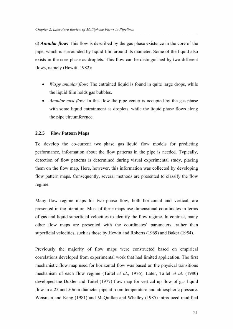
Chapter 2. Literature Review of Multiphase Flows in Pipelines _______________________________________________________________________________________________________
21
d) Annular flow: This flow is described by the gas phase existence in the core of the
pipe, which is surrounded by liquid film around its diameter. Some of the liquid also
exists in the core phase as droplets. This flow can be distinguished by two different
flows, namely (Hewitt, 1982):
Wispy annular flow: The entrained liquid is found in quite large drops, while
the liquid film holds gas bubbles.
Annular mist flow: In this flow the pipe center is occupied by the gas phase
with some liquid entrainment as droplets, while the liquid phase flows along
the pipe circumference.
2.2.5 Flow Pattern Maps
To develop the co-current two–phase gas–liquid flow models for predicting
performance, information about the flow patterns in the pipe is needed. Typically,
detection of flow patterns is determined during visual experimental study, placing
them on the flow map. Here, however, this information was collected by developing
flow pattern maps. Consequently, several methods are presented to classify the flow
regime.
Many flow regime maps for two–phase flow, both horizontal and vertical, are
presented in the literature. Most of these maps use dimensional coordinates in terms
of gas and liquid superficial velocities to identify the flow regime. In contrast, many
other flow maps are presented with the coordinates’ parameters, rather than
superficial velocities, such as those by Hewitt and Roberts (1969) and Baker (1954).
Previously the majority of flow maps were constructed based on empirical
correlations developed from experimental work that had limited application. The first
mechanistic flow map used for horizontal flow was based on the physical transitions
mechanism of each flow regime (Taitel et al., 1976). Later, Taitel et al. (1980)
developed the Dukler and Taitel (1977) flow map for vertical up flow of gas-liquid
flow in a 25 and 50mm diameter pipe at room temperature and atmospheric pressure.
Weisman and Kang (1981) and McQuillan and Whalley (1985) introduced modified
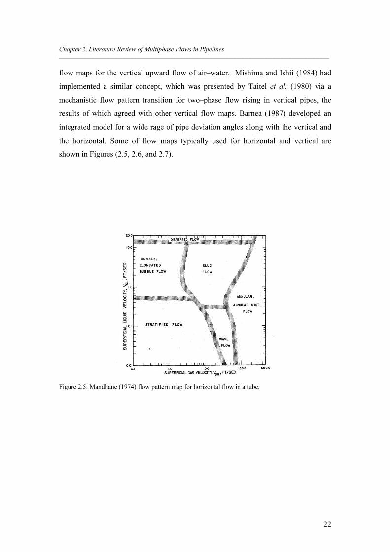
Chapter 2. Literature Review of Multiphase Flows in Pipelines _______________________________________________________________________________________________________
22
flow maps for the vertical upward flow of air–water. Mishima and Ishii (1984) had
implemented a similar concept, which was presented by Taitel et al. (1980) via a
mechanistic flow pattern transition for two–phase flow rising in vertical pipes, the
results of which agreed with other vertical flow maps. Barnea (1987) developed an
integrated model for a wide rage of pipe deviation angles along with the vertical and
the horizontal. Some of flow maps typically used for horizontal and vertical are
shown in Figures (2.5, 2.6, and 2.7).
Figure 2.5: Mandhane (1974) flow pattern map for horizontal flow in a tube.
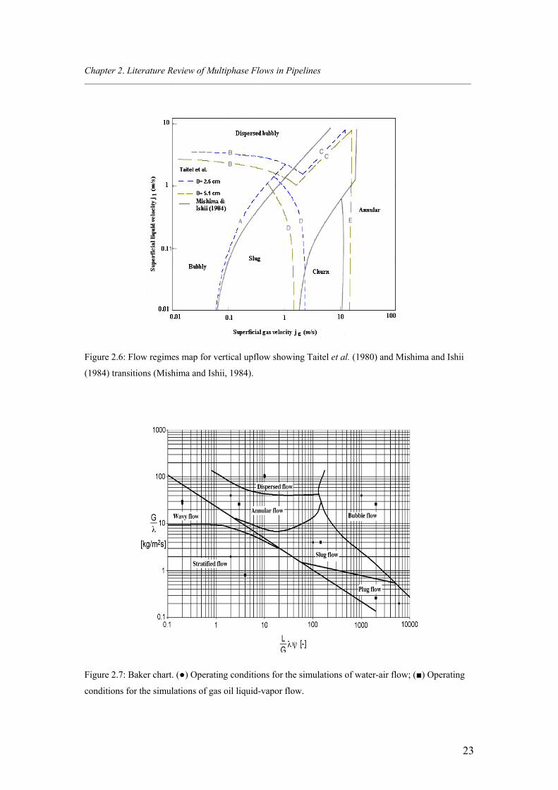
Chapter 2. Literature Review of Multiphase Flows in Pipelines _______________________________________________________________________________________________________
23
Figure 2.6: Flow regimes map for vertical upflow showing Taitel et al. (1980) and Mishima and Ishii
(1984) transitions (Mishima and Ishii, 1984).
Figure 2.7: Baker chart. (●) Operating conditions for the simulations of water-air flow; (■) Operating
conditions for the simulations of gas oil liquid-vapor flow.
Chapter 2. Literature Review of Multiphase Flows in Pipelines _______________________________________________________________________________________________________
24
2.3 Liquid Holdup and Pressure Drop in Horizontal Pipelines
2.3.1 Liquid Holdup Correlations of Adiabatic Two–phase Flow
In order to study co-current two–phase flows in a horizontal pipe, liquid holdup is one
of the important factors to consider. In practice, the two–phase velocities do not move
at the same rate, therefore the in-situ volume fraction will be completely different
from the inlet volume fraction.
In the 1940s, researchers began to investigate the pressure drop and liquid holdup in
the multiphase flow. Since then, data has been gathered for pressure drop and liquid
holdup of two-phase flow for various pipeline inclinations, horizontal and vertical.
The study of multiphase flow in pipelines has proven to be a very difficult concept
because of various parameters, such as pipe roughness, pipe incline angle, pipe
diameter, surface tension, two-phase densities, viscosities, velocities and the initial
liquid fraction.
At a single phase flow, some of the factors such as flow regime characteristics and
liquid holdup are not included. Based on the collected data, many empirical
correlations have been developed, but they remain restricted for use in some
applications due to accuracy. Moreover, these correlations cannot be extrapolated to
the data rather than information that is based on or is valid for particular flow
conditions. Different studies have been performed and a model has been developed to
predict the pressure drop and liquid holdup. Table (2.1) shows different correlations
that have been proposed for liquid holdup predictions.
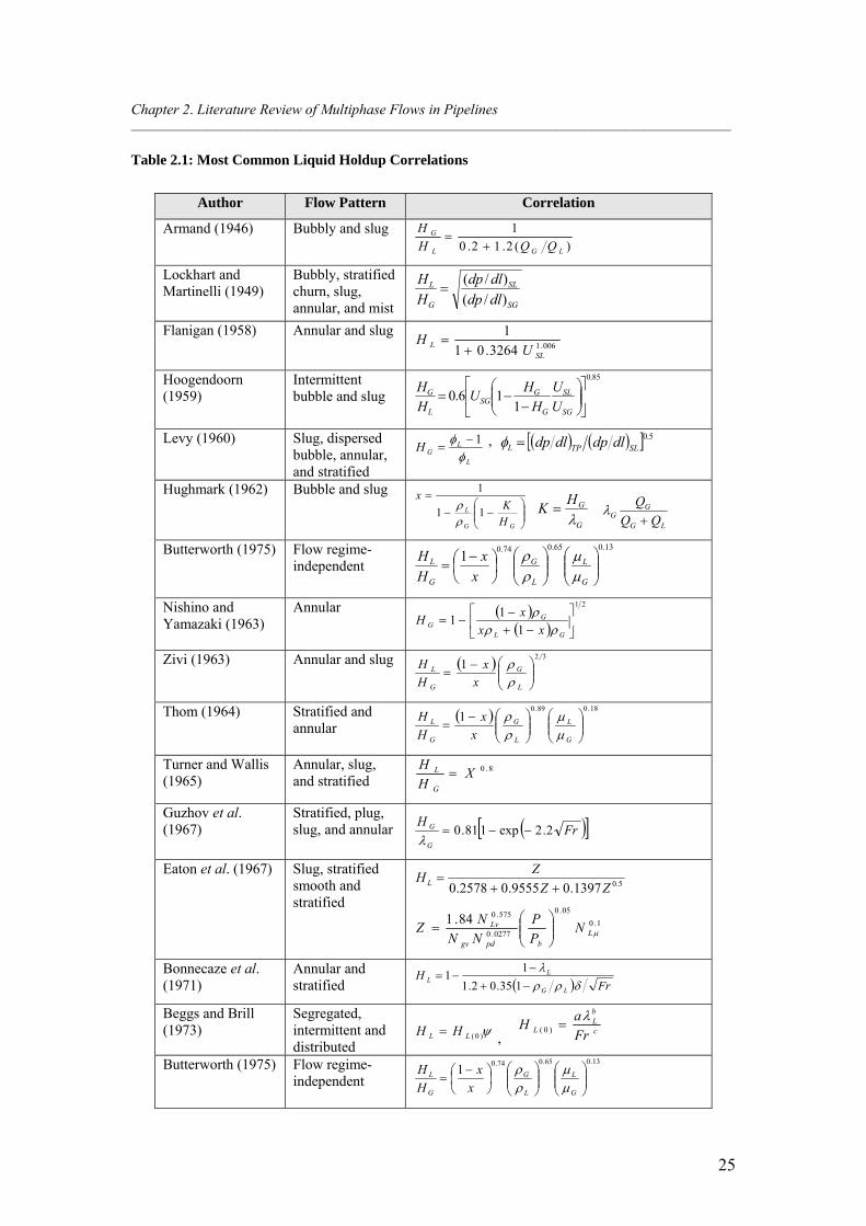
Chapter 2. Literature Review of Multiphase Flows in Pipelines _______________________________________________________________________________________________________
25
Table 2.1: Most Common Liquid Holdup Correlations
Author Flow Pattern Correlation
Armand (1946) Bubbly and slug )(2.12.0
1
LGL
G
QQH
H
Lockhart and Martinelli (1949)
Bubbly, stratified churn, slug, annular, and mist SG
SL
G
L
dldp
dldp
H
H
)/(
)/(
Flanigan (1958) Annular and slug 006.13264.01
1
SLL U
H
Hoogendoorn (1959)
Intermittent bubble and slug
85.0
116.0
SG
SL
G
GSG
L
G
U
U
H
HU
H
H
Levy (1960) Slug, dispersed bubble, annular, and stratified
L
LGH
1
, 5.0SLTPL dldpdldp
Hughmark (1962) Bubble and slug
GG
L
H
Kx
11
1
G
GHK
LG
GG QQ
Q
Butterworth (1975) Flow regime-independent
13.065.074.01
G
L
L
G
G
L
x
x
H
H
Nishino and Yamazaki (1963)
Annular
21
1
11
GL
GG xx
xH
Zivi (1963) Annular and slug 321
L
G
G
L
x
x
H
H
Thom (1964) Stratified and annular
18.089.01
G
L
L
G
G
L
x
x
H
H
Turner and Wallis (1965)
Annular, slug, and stratified
8.0XH
H
G
L
Guzhov et al. (1967)
Stratified, plug, slug, and annular Fr
H
G
G 2.2exp181.0
Eaton et al. (1967) Slug, stratified smooth and stratified
5.01397.09555.02578.0 ZZ
ZH L
1.0
05.0
0277.0
575.084.1L
bpdgv
Lv NP
P
NN
NZ
Bonnecaze et al. (1971)
Annular and stratified Fr
HLG
LL
135.02.1
11
Beggs and Brill (1973)
Segregated, intermittent and distributed
)0(LL HH , c
bL
L Fr
aH
)0(
Butterworth (1975) Flow regime-independent
13.065.074.01
G
L
L
G
G
L
x
x
H
H
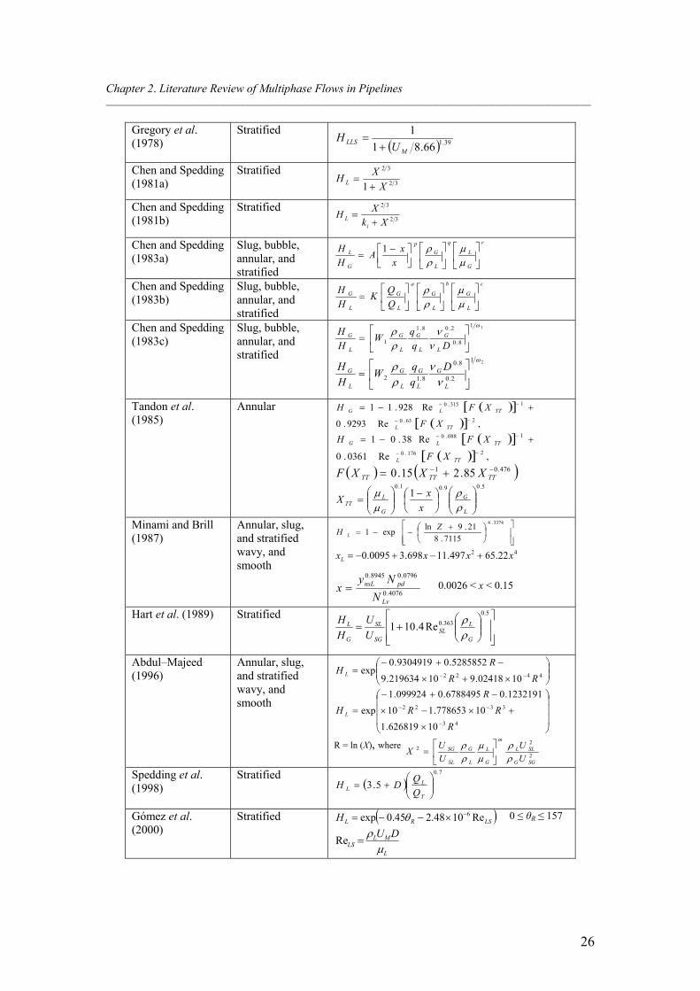
Chapter 2. Literature Review of Multiphase Flows in Pipelines _______________________________________________________________________________________________________
26
Gregory et al. (1978)
Stratified
39.166.81
1
M
LLSU
H
Chen and Spedding (1981a)
Stratified 32
32
1 X
XH L
Chen and Spedding (1981b)
Stratified 32
32
Xk
XH
iL
Chen and Spedding (1983a)
Slug, bubble, annular, and stratified
r
G
L
q
L
G
p
G
L
x
xA
H
H
1
Chen and Spedding (1983b)
Slug, bubble, annular, and stratified
c
L
G
b
L
G
a
L
G
L
G
Q
QK
H
H
Chen and Spedding (1983c)
Slug, bubble, annular, and stratified
11
8.0
2.08.1
1
Dq
qW
H
H
L
G
L
G
L
G
L
G
21
2.0
8.0
8.12
L
G
L
G
L
G
L
G D
q
qW
H
H
Tandon et al. (1985)
Annular ,Re9293.0
Re928.11263.0
1315.0
TTL
TTLG
XF
XFH
,Re0361.0
Re38.012176.0
1088.0
TTL
TTLG
XF
XFH
476.01 85.215.0 TTTTTT XXXF 5.09.01.0
1
L
G
G
LTT x
xX
Minami and Brill (1987)
Annular, slug, and stratified wavy, and smooth
3374.4
7115.821.9ln
exp1Z
H L
42 22.65497.11698.30095.0 xxxxL
4076.0
0796.08945.0
Lv
pdnsL
N
Nyx 0.0026 < x < 0.15
Hart et al. (1989) Stratified
5.0
363.0Re4.101G
LSL
SG
SL
G
L
U
U
H
H
Abdul–Majeed (1996)
Annular, slug, and stratified wavy, and smooth
4422 1002418.910219634.9
5285852.09304919.0exp
RR
RH L
43
3322
10626819.1
10778653.110
1232191.06788495.0099924.1
exp
R
RR
R
H L
R = ln (X), where 2
22
SGG
SLL
m
G
L
L
G
SL
SG
U
U
U
UX
Spedding et al. (1998)
Stratified
7.0
5.3
T
LL Q
QDH
Gόmez et al. (2000)
Stratified LSRLH Re1048.245.0exp 6 0 ≤ θR ≤ 157
L
MLLS
DU
Re
Chapter 2. Literature Review of Multiphase Flows in Pipelines _______________________________________________________________________________________________________
27
2.3.2 Pressure Drop Correlations of Adiabatic Two–phase Flow
The pressure drop of two–phase flow depends on a different number of independent
factors, such as conduit geometry, mass flux, conduit orientation (i.e. vertical,
horizontal or inclined), two–phase properties (i.e. density, viscosity), volume fraction
of each phase, flow direction (i.e. down flow, upward flow, or counter-current flow),
and flow regimes. Moreover, in practical engineering applications, two–phase flow
processes can be classified into different physical situations, such as adiabatic and
diabatic, or in different flow components such as one–phase, two–phase or multi–
phase. The pressure drop of these several applications has to be correlated for
availability.
A number of correlations for two–phase pressure drop in a horizontal co–current flow
can be found in the literature. Most of them in practice are realistically only valid for
a limited range of parameters. Mechanistic models are derived based on specific
assumptions, and careful assessment of a particular system is required to ensure that
these assumptions are in close agreement.
The two–phase flow pressure drop correlations can be categorized into four groups.
These are:
1- Empirical correlations based on a homogenous model.
2- Empirical correlations based on a two–phase friction multiplier model.
3- Direct empirical models.
4- Flow regime specific models.
Most of the widely utilized and frequently referred to correlations of these classes are
given in Table (2.2).
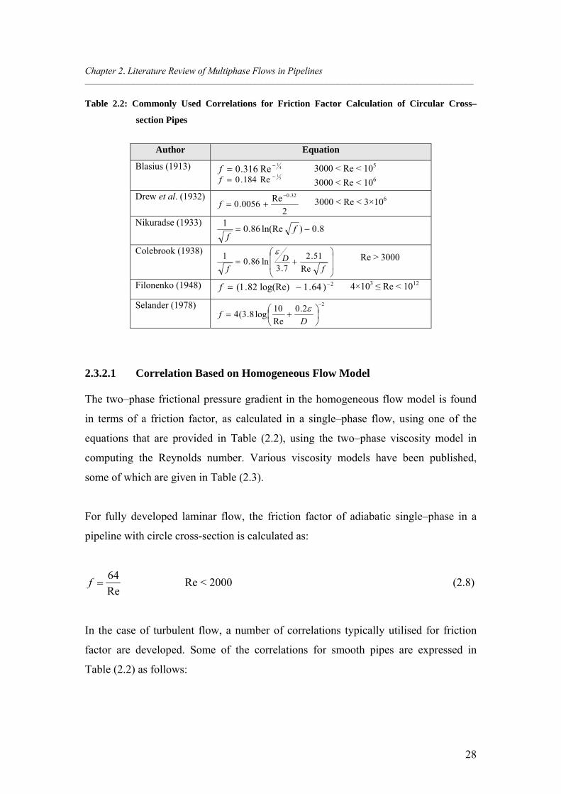
Chapter 2. Literature Review of Multiphase Flows in Pipelines _______________________________________________________________________________________________________
28
Table 2.2: Commonly Used Correlations for Friction Factor Calculation of Circular Cross–
section Pipes
Author Equation
Blasius (1913) 41
Re316.0 f 3000 < Re < 105
51
Re184.0 f 3000 < Re < 106
Drew et al. (1932)
2
Re0056.0
32.0
f 3000 < Re < 3×10⁶
Nikuradse (1933) 8.0)ln(Re86.0
1 f
f
Colebrook (1938)
fD
f Re
51.2
7.3ln86.0
1 Re > 3000
Filonenko (1948) 2)64.1log(Re)82.1( f 4×10³ ≤ Re < 1012
Selander (1978) 22.0
Re
10log8.3(4
Df
2.3.2.1 Correlation Based on Homogeneous Flow Model
The two–phase frictional pressure gradient in the homogeneous flow model is found
in terms of a friction factor, as calculated in a single–phase flow, using one of the
equations that are provided in Table (2.2), using the two–phase viscosity model in
computing the Reynolds number. Various viscosity models have been published,
some of which are given in Table (2.3).
For fully developed laminar flow, the friction factor of adiabatic single–phase in a
pipeline with circle cross-section is calculated as:
Re
64f Re < 2000 (2.8)
In the case of turbulent flow, a number of correlations typically utilised for friction
factor are developed. Some of the correlations for smooth pipes are expressed in
Table (2.2) as follows:
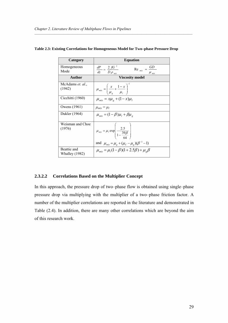
Chapter 2. Literature Review of Multiphase Flows in Pipelines _______________________________________________________________________________________________________
29
Table 2.3: Existing Correlations for Homogeneous Model for Two–phase Pressure Drop
Category Equation
Homogeneous Mode
mixD
fG
dz
dP
22
mixmix
GD
Re
Author Viscosity model
McAdams et. al., (1942)
1
1
lgmix
xx
Cicchitti (1960) lgmix xx )1(
Owens (1961) μmix = μl
Dukler (1964) glmix )1(
Weisman and Choe (1976)
64
391
5.2exp lmix
and )1)(( 1 gCgmix
Beattie and Whalley (1982)
glmix )5.21)(1(
2.3.2.2 Correlations Based on the Multiplier Concept
In this approach, the pressure drop of two–phase flow is obtained using single–phase
pressure drop via multiplying with the multiplier of a two–phase friction factor. A
number of the multiplier correlations are reported in the literature and demonstrated in
Table (2.4). In addition, there are many other correlations which are beyond the aim
of this research work.
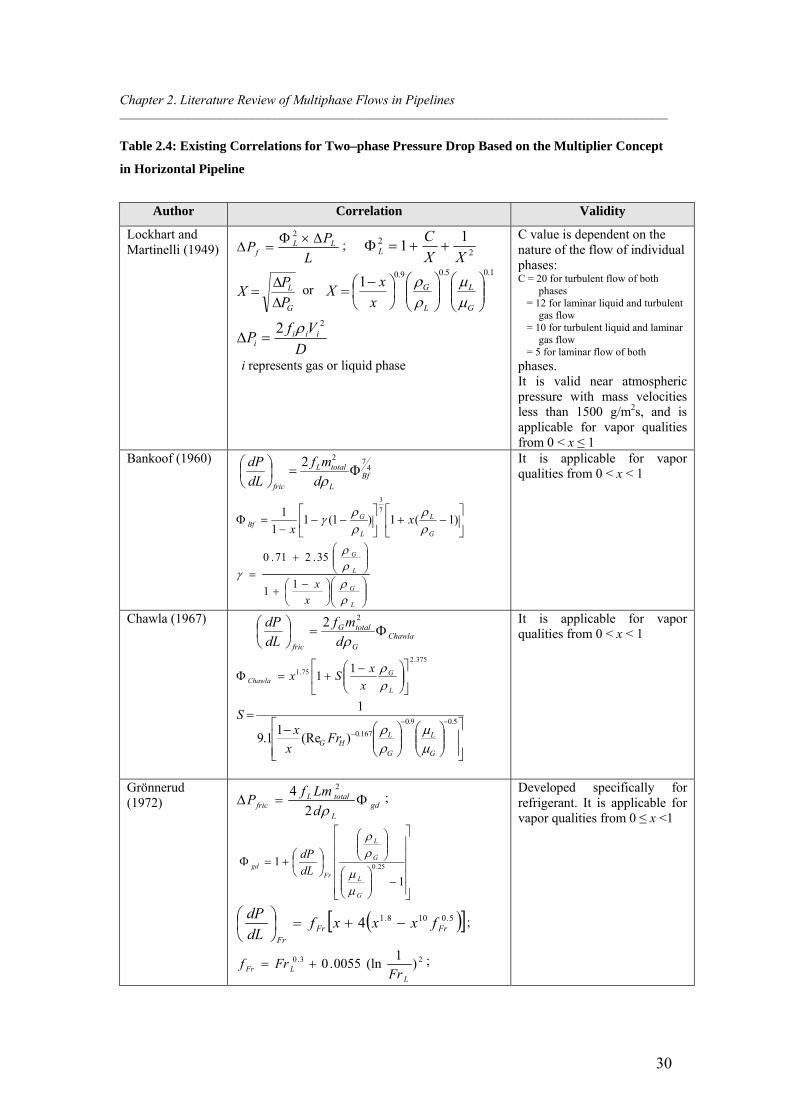
Chapter 2. Literature Review of Multiphase Flows in Pipelines _______________________________________________________________________________________________________
30
Table 2.4: Existing Correlations for Two–phase Pressure Drop Based on the Multiplier Concept
in Horizontal Pipeline
Author Correlation Validity
Lockhart and Martinelli (1949)
L
PP LL
f
2
; 2
2 11
XX
CL
G
L
P
PX
or
1.05.09.01
G
L
L
G
x
xX
D
VfP iii
i
22
i represents gas or liquid phase
C value is dependent on the nature of the flow of individual phases: C = 20 for turbulent flow of both
phases = 12 for laminar liquid and turbulent
gas flow = 10 for turbulent liquid and laminar
gas flow = 5 for laminar flow of both
phases. It is valid near atmospheric pressure with mass velocities less than 1500 g/m2s, and is applicable for vapor qualities from 0 < x ≤ 1
Bankoof (1960) 4
722Bf
L
totalL
fric d
mf
dL
dP
)1(1)1(1
1
1 7
3
G
L
L
GBf x
x
L
G
L
G
x
x
1
1
35.271.0
It is applicable for vapor qualities from 0 < x < 1
Chawla (1967)
ChawlaG
totalG
fric d
mf
dL
dP
22
375.2
75.1 11
L
GChawla x
xSx
5.09.0
167.0)(Re1
1.9
1
G
L
G
LHG Fr
x
xS
It is applicable for vapor qualities from 0 < x < 1
Grönnerud (1972) gd
L
totalLfric d
LmfP
2
4 2
;
1
1 25.0
G
L
G
L
Frgd dL
dP
5.0108.14 FrFrFr
fxxxfdL
dP
;
23.0 )1
(ln0055.0L
LFr FrFrf ;
Developed specifically for refrigerant. It is applicable for vapor qualities from 0 ≤ x <1
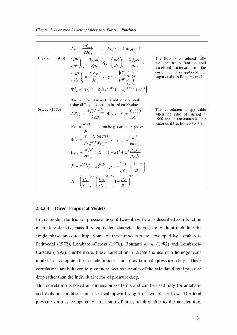
Chapter 2. Literature Review of Multiphase Flows in Pipelines _______________________________________________________________________________________________________
31
2
2
L
totalL gd
mFr
if FrL ≥ 1 then fFr = 1
Chisholm (1973) 2
22Ch
L
tL
fric d
mf
dz
dP
,
G
tG
G d
mf
dz
dP
22
,
G
tL
L d
mf
dz
dP
22
;
L
G
dzdP
dzdP
Y 2
nnnCh xxBxY 22/)2(2/)2(22 )1()1(1
B is function of mass flux and is calculated using different equations based on Y values
The flow is considered fully turbulent Re < 2000 to void undefined interval in the correlation. It is applicable for vapor qualities from 0 ≤ x ≤ 1
Friedel (1979) 2
2
2
4fr
L
totalLfric d
LmfP
;
25.0Re
079.0
iif
i
ti
dm
Re i can be gas or liquid phase
035.0045.02 24.3
LHfr WeFr
FHE ;
2
2
H
tH gd
mFr
H
tL
dmWe
2
, LG
GL
f
fxxE
22)1(
224.078.0 )1( xxF ,
11
LGH
xx
7.019.091.0
1
L
G
L
G
G
LH
This correlation is applicable when the ratio of (μL/μG) < 1000 and is recommended for vapor qualities from 0 ≤ x ≤ 1
2.3.2.3 Direct Empirical Models
In this model, the friction pressure drop of two–phase flow is described as a function
of mixture density, mass flux, equivalent diameter, length, etc. without including the
single phase pressure drop. Some of these models were developed by Lombardi–
Pedrocchi (1972), Lombardi–Ceresa (1978), Bonfanti et al. (1982) and Lombardi–
Carsana (1992). Furthermore, these correlations indicate the use of a homogeneous
model to compute the accelerational and gravitational pressure drop. These
correlations are believed to give more accurate results of the calculated total pressure
drop rather than the individual terms of pressure drop.
This correlation is based on dimensionless terms and can be used only for adiabatic
and diabatic conditions in a vertical upward single or two–phase flow. The total
pressure drop is computed via the sum of pressure drop due to the acceleration,
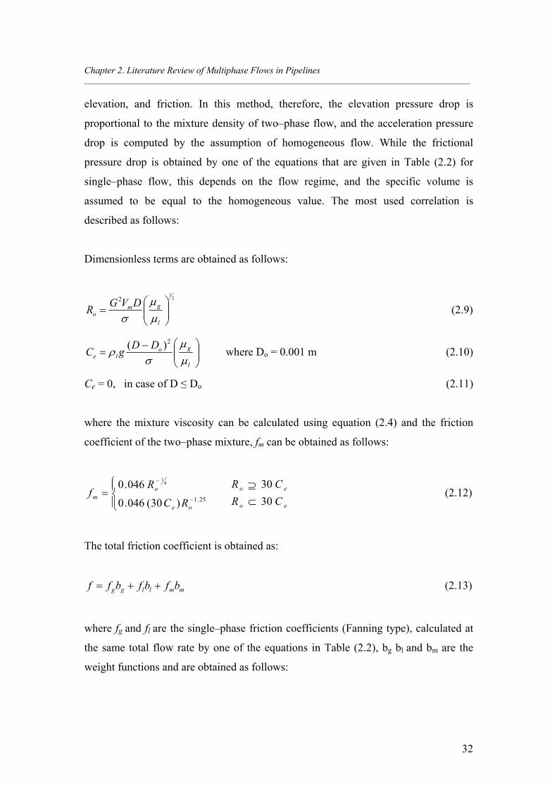
Chapter 2. Literature Review of Multiphase Flows in Pipelines _______________________________________________________________________________________________________
32
elevation, and friction. In this method, therefore, the elevation pressure drop is
proportional to the mixture density of two–phase flow, and the acceleration pressure
drop is computed by the assumption of homogeneous flow. While the frictional
pressure drop is obtained by one of the equations that are given in Table (2.2) for
single–phase flow, this depends on the flow regime, and the specific volume is
assumed to be equal to the homogeneous value. The most used correlation is
described as follows:
Dimensionless terms are obtained as follows:
21
2
l
gmo
DVGR
(2.9)
l
gole
DDgC
2)( where Do = 0.001 m (2.10)
Ce = 0, in case of D ≤ Do (2.11)
where the mixture viscosity can be calculated using equation (2.4) and the friction
coefficient of the two–phase mixture, fm can be obtained as follows:
25.1)30(046.0
046.0 41
oe
om
RC
Rf
eo
eo
CR
CR
30
30
(2.12)
The total friction coefficient is obtained as:
mmllgg bfbfbff (2.13)
where fg and fl are the single–phase friction coefficients (Fanning type), calculated at
the same total flow rate by one of the equations in Table (2.2), bg bl and bm are the
weight functions and are obtained as follows:
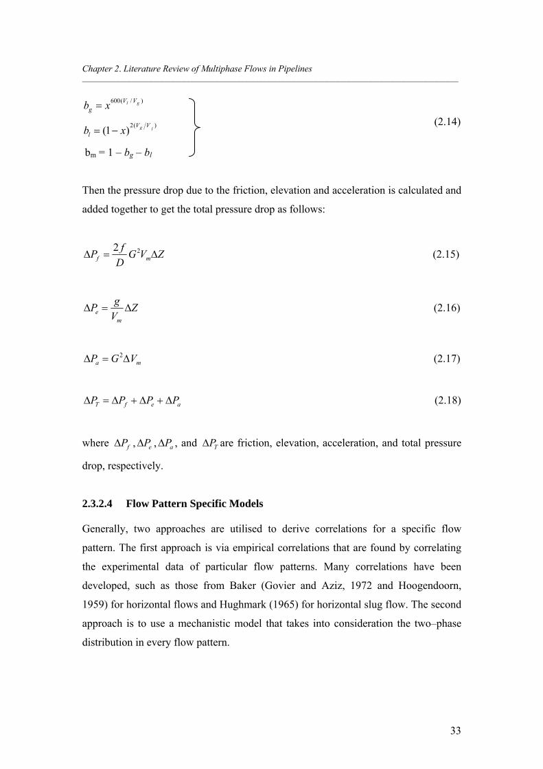
Chapter 2. Literature Review of Multiphase Flows in Pipelines _______________________________________________________________________________________________________
33
)/(600 gl VVg xb
)(2)1( lg VV
l xb
bm = 1 – bg – bl
Then the pressure drop due to the friction, elevation and acceleration is calculated and
added together to get the total pressure drop as follows:
ZVGD
fP mf 22
(2.15)
ZV
gP
me (2.16)
ma VGP 2 (2.17)
aefT PPPP (2.18)
where fP , eP , aP , and TP are friction, elevation, acceleration, and total pressure
drop, respectively.
2.3.2.4 Flow Pattern Specific Models
Generally, two approaches are utilised to derive correlations for a specific flow
pattern. The first approach is via empirical correlations that are found by correlating
the experimental data of particular flow patterns. Many correlations have been
developed, such as those from Baker (Govier and Aziz, 1972 and Hoogendoorn,
1959) for horizontal flows and Hughmark (1965) for horizontal slug flow. The second
approach is to use a mechanistic model that takes into consideration the two–phase
distribution in every flow pattern.
(2.14)
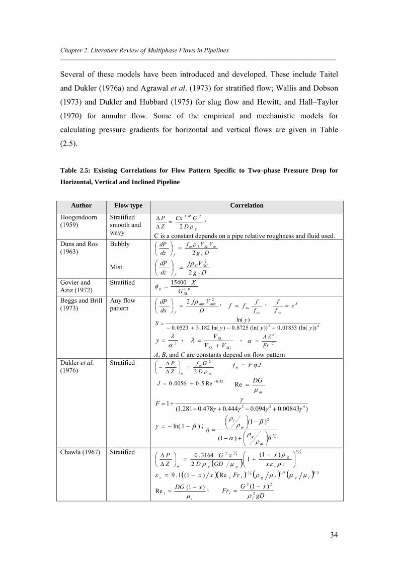
Chapter 2. Literature Review of Multiphase Flows in Pipelines _______________________________________________________________________________________________________
34
Several of these models have been introduced and developed. These include Taitel
and Dukler (1976a) and Agrawal et al. (1973) for stratified flow; Wallis and Dobson
(1973) and Dukler and Hubbard (1975) for slug flow and Hewitt; and Hall–Taylor
(1970) for annular flow. Some of the empirical and mechanistic models for
calculating pressure gradients for horizontal and vertical flows are given in Table
(2.5).
Table 2.5: Existing Correlations for Flow Pattern Specific to Two–phase Pressure Drop for
Horizontal, Vertical and Inclined Pipeline
Author Flow type Correlation
Hoogendoorn (1959)
Stratified smooth and wavy
gD
GCx
Z
P
2
245.1
,
C is a constant depends on a pipe relative roughness and fluid used. Duns and Ros (1963)
Bubbly Mist
Dg
VVf
dz
dP
C
mSLLm
f 2
Dg
Vf
dz
dP
C
SGG
f 2
2
Govier and Aziz (1972)
Stratified 8.0
15400
SLg G
X
Beggs and Brill (1973)
Any flow pattern D
Vf
dx
dP mixmix
f
22
,
nsns f
fff , S
ns
ef
f
42 ))(ln(01853.0))(ln(8725.0)ln(182.30523.0
)ln(
yyy
yS
2
y , SGSL
SL
VV
V
,
C
B
Fr
A
A, B, and C are constants depend on flow pattern Dukler et al. (1976)
Stratified
m
m
m D
Gf
Z
P
2
2
JFf m
32.0Re5.00056.0 J m
DG
Re
)00843.0094.0444.0478.0281.1(1
432
F
)1ln( ;
2
)1(
)1( 2
m
g
m
l
Chawla (1967) Stratified
8
19
47 )1(
12
3164.0 2
lc
g
ggm x
x
GDD
xG
Z
P
5.09.061
Re)1(1.9 lglgllc Frxx
ll
xDG
)1(
Re
; gD
xGFr
ll 2
22 )1(
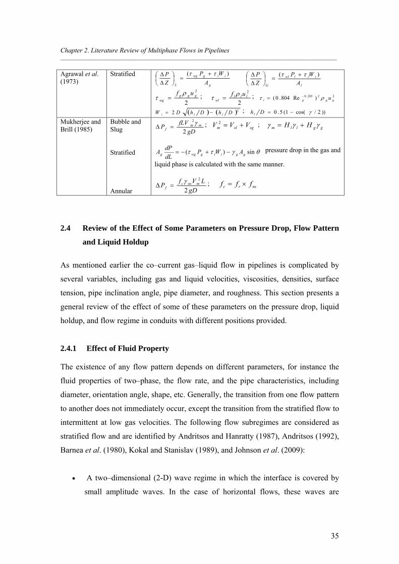
Chapter 2. Literature Review of Multiphase Flows in Pipelines _______________________________________________________________________________________________________
35
Agrawal et al. (1973)
Stratified
g
iigwg
L A
WP
Z
P )(
l
iilwl
G A
WP
Z
P )(
2
2ggg
wg
uf ;
2
2lll
wl
uf ; 22285.0 )Re804.0( gggi u
22 DhDhDW lli ; ))2/cos(1(5.0 Dh l
Mukherjee and Brill (1985)
Bubble and Slug Stratified Annular
gD
fLVP mm
f 2
2 ; sgslm VVV 2 ; ggllm HH
sin)( ggiigwgg AWPdL
dPA pressure drop in the gas and
liquid phase is calculated with the same manner.
gD
LVfP mnsc
f 2
2 ; nsrc fff
2.4 Review of the Effect of Some Parameters on Pressure Drop, Flow Pattern
and Liquid Holdup
As mentioned earlier the co–current gas–liquid flow in pipelines is complicated by
several variables, including gas and liquid velocities, viscosities, densities, surface
tension, pipe inclination angle, pipe diameter, and roughness. This section presents a
general review of the effect of some of these parameters on the pressure drop, liquid
holdup, and flow regime in conduits with different positions provided.
2.4.1 Effect of Fluid Property
The existence of any flow pattern depends on different parameters, for instance the
fluid properties of two–phase, the flow rate, and the pipe characteristics, including
diameter, orientation angle, shape, etc. Generally, the transition from one flow pattern
to another does not immediately occur, except the transition from the stratified flow to
intermittent at low gas velocities. The following flow subregimes are considered as
stratified flow and are identified by Andritsos and Hanratty (1987), Andritsos (1992),
Barnea et al. (1980), Kokal and Stanislav (1989), and Johnson et al. (2009):
A two–dimensional (2-D) wave regime in which the interface is covered by
small amplitude waves. In the case of horizontal flows, these waves are
Chapter 2. Literature Review of Multiphase Flows in Pipelines _______________________________________________________________________________________________________
36
generated due to the pressure variations in the phase with the wave slop. They
increase in amplitude and in wavelength as they propagate downstream.
A Kelvin–Helmholtz (K–H) wave region with large amplitude irregular
waves, also known as a roll wave. These waves are associated with pressure
variations in phase with the wave height (K–H instability).
An Atomization region, where droplets or liquid filaments are broken off
from the crests of the K–H waves and deposited on the pipe wall. Moreover,
the liquid begins to climb up the pipe wall and the average shape is not
approximated by a flat horizontal plane, at least for small conduit diameters
(Dpipe < 5 cm) and low viscosity liquids.
The effect of fluid properties is considered as one of the significant parameters in
two–phase flow phenomena, and it directly influences flow pattern, pressure drop, and
liquid holdup. Over the past five decades, several authors have studied this effect
(Hoogendoorn, 1959, Weisman et al., 1979, and Andritsos, 1986). One of the most
frequently examined fluid properties is liquid viscosity. Hoogendoorn (1959)
performed a two–phase experiment that utilized air–water and air–oil in horizontal
smooth pipelines with an inner diameter range from 0.024 to 0.14 m, and rough pipes
with an inside diameter of 0.05 m under various operating conditions.
Based on the results obtained from this experiment, Hoogendoorn found that the pipe
diameter and liquid viscosity had no significant effect on the transition among the
flow patterns. This finding was contradicted later by Andritsos (1986) and Carson
(1989). Hoogendoorn (1959) noted that stratified flow took place at higher air flow
rates with air–oil mixtures because of the surface tension effect. Moreover, a few
years later, Hoogendoorn (1961) investigated the effect of gas density using
superheated Freon–11 as the gas fluid. The increase in gas density was reported not to
have a significant influence on the transition to slug or plug flow, but reduces
drastically the onset of atomization. Hanratty and Hershman (1961) studied the
influence of fluid physical properties on the flow pattern in a horizontal pipeline.
They found that the increase of liquid viscosity slightly reduces the needed gas
Chapter 2. Literature Review of Multiphase Flows in Pipelines _______________________________________________________________________________________________________
37
velocity for transition to roll ripples, while adding the surfactant reduced the
disturbance of the surface.
The impact of fluid properties on two–phase flow patterns in horizontal conduits was
also investigated by Weisman et al. (1979). He found that the flow pattern maps for
glycerol–water solutions were slightly different from air–water system flow maps. A
similar trend was noted when using a surface active agent (Aliquat 221), with the only
difference being that the smooth–wavy transition was noted to take place at higher gas
flow rates.
In the experiments with boiling Freon–113, the gas density fluctuated at pressure
values of 1 and 4 atm, but the effect of the density was quite complicated compared to
liquid viscosity and surface tension, which were simultaneously significantly
decreased with respect to the air–water case. Andritsos and Hanratty (1987) and
Andritsos et al. (1989) performed a systematic experimental study of the effect of
liquid viscosity ranging from 0.001 to 0.08 Pa–s, on flow pattern. They reported that
increasing liquid viscosity with a lower liquid loading was required for the slug
transition at low gas flow rates. Furthermore, the region with two–dimensional waves
reduces in size with increasing viscosity, while the transition to roll waves is only
slightly affected.
The impact of gas density on the flow behaviour in gas–liquid flow in horizontal and
inclined pipelines has been experimentally investigated by Christina et al. (2011)
using air–carbon dioxide–helium fluid. They found that the gas density strongly
affects the transition of smooth to 2-D waves and later to K–H waves. Furthermore,
the increase of gas density destabilized the flow and the transition to 2-D and K–H
waves that occur at low gas velocities. The same observation also was reported for the
transition to the atomization region and annular flow patterns that are directly related
to the roll wave’s onset.
Chapter 2. Literature Review of Multiphase Flows in Pipelines _______________________________________________________________________________________________________
38
2.4.2 Effect of Surface Tension
A number of limited experimental results have been shown on the effect of surface
agents on two–phase flow parameters (liquid holdup, pressure drop). This is in
comparison to single–phase flow, where considerable attention has been focussed.
The effect of surface tension reduction on flow pattern, liquid holdup and pressure
drop has been investigated and the outcome of these studies is summarized as follows.
2.4.2.1 Effect of Surfactant on Flow Pattern
The reduction of surface tension is one of the factors that can influence the flow
pattern. Hand et al. (1991) conducted a two–phase flow of air–water and air–
surfactant solution in a horizontal “Perspex” pipe with 0.0935m diameter and around
13m in length. The air and water flow rates were delivered in the system up to 0.13
and 0.003m3/s, respectively. They performed a sensitivity analysis of the effect of
surface tension reduction on the flow pattern, liquid holdup and pressure drop. They
added a small amount of surface–active agent with different liquid flow rates of
1×10⁻⁴ m3/s, 3.33×10⁻⁴ m3/s, and 1×10⁻³ m3/s, respectively. The stratified flow pattern
typically was observed at higher rates of air flow.
This is a well–known phenomenon and was given by Franklin (1965), Davies and
Rose (1965) and Miles (1966) who noted that surface–active agents dampen capillary
waves in a closed basin. That saturated air created some waves on the liquid film
flowing on a flat plate was also seen by Craik (1968). Van Rossum (1959) observed
that at fully developed velocity, regular two–dimensional waves (i.e. stratified with
wave) occurred on the water film of 0.6 mm thickness in a horizontal rectangular pipe
and increased from 7 to 10 m/s via adding the Teepol surfactant. Thwaites et al.
(1976) studied the flow down of two–phase air–water flow co–current annular flows
with and without surfactant (Separan AR30) in 0.0318 m diameter and 10m long.
They concluded that the addition of surfactant (100 ppm) to water led to surface
waves becoming moist. As a result of that the roll wave frequency decreases by half
and increases the mean film thickness.
Chapter 2. Literature Review of Multiphase Flows in Pipelines _______________________________________________________________________________________________________
39
These results for annular flow have a similar behaviour to those observed in the study
by Hand et al. (1991) for stratified category flow patterns. The techniques employed
in Hand et al (1991) were unable to identify any change in the roll waves’ frequency
due to the addition of the surfactant (Chemtreat 271).
Hanratty and Hershman (1961) examined the effect of surfactant using (sodium lauyrl
sulphate agent) on the transition to the roll wave flow in a rectangular pipeline. They
noted that the stratified flow pattern was developed and the transition to stratified plus
roll waves can take place from a smooth stratified liquid film. Furthermore, based on
their results and suggestion, the reduction in the stratified with waves region could be
due to the increase of flow rate at which energy is dissipated to the liquid phase, or to
the increased the viscosity of the film surface. However, the effect of adding
surfactant was noted to be insignificant on the transition to stratified with roll waves.
Hanratty and Hershman (1961) also noted that the surface tension has no effect on the
transition to roll wave flow. Moreover, Weisman et al. (1979) noted that the use of a
surface active agent (Aliquat 221) has a slight impact on the flow maps of glycerol–
water solution in comparison with the air–water flow maps, with the only difference
at high gas flow rates where the smooth–wavy transition takes place.
Christina et al. (2011) investigated the reduction of surface tension of water from
0.072 to 0.035 N/m using a butanol aqueous solution on the flow pattern. It was
reported that at the same liquid flow rate, a significant reduction for gas flow rate is
needed for the onset of the first disturbances. Both transitions of smooth and later to
2-D and K–H waves respectively are moved to lower gas flow rates, therefore the 2-D
wave transition is more obviously affected.
2.4.2.2 The Effect of Surfactant on Holdup
Minami et al. (1987) studied the effect of surfactant on two–phase liquid holdup in a
horizontal pipe about 400 m long and 0.078 m diameter. Three different mixtures of
two–phase flow were utilized (air–kerosene, air–water, and air–water–surfactant). For
a very foamy mixture with very high two–phase superficial velocities, a crucial
Chapter 2. Literature Review of Multiphase Flows in Pipelines _______________________________________________________________________________________________________
40
decline in the liquid holdup was noted, while at very low velocity experiments the
liquid holdup was not affected.
It was concluded that at high turbulence, generated due to high superficial velocities
with very foamy mixture, small bubbles of air were expected to form in the liquid
phase, which leads to a decrease in the actual liquid holdup. The existence of the foam
near the interface therefore would be most likely to increase the interfacial stress,
resulting in a decrease in the difference of slip velocity between the phases and thus
reducing the final liquid holdup. In contrast to the results of air–water, and air–water
with surfactant, they reported that the effect of surface tension was insignificant. In
addition, at non–foamy water with surfactant mixture, the liquid holdup stayed
constant compared to air–water flow liquid holdup.
Hand et al. (1991) has classified the effect of surfactant on holdup based on the gas
flow rates. First of all, when the gas volumetric flow rate is less than 0.02 m3/s the
liquid holdup was not influenced via the reduction in surface tension where the flow
pattern was observed as a smooth stratified flow. When the gas volumetric flow rate is
increased to between 0.02 and 0.07 m3/s a significant increase in the liquid holdup
was noted, and different flow patterns were observed in this flow rate range. The
observed flow patterns are stratified with wave, roll wave, and long roll wave with
droplet. At gas volumetric flow rates above 0.08 m3/s there was no significant
difference between water and surfactant solution holdup. Also different flow patterns
were observed, such as stratified roll wave with droplet and film with droplet.
In addition, Hart et al. (1989) studied the effect of surface tension reduction (from
0.072 to 0.046 N/m) on two–phase air–water flow in a horizontal “copper” pipeline
with 0.051 m diameter and around 17 m long. They conducted experimental work
considering a small amount of liquid, similar to conditions found in gas condensate
pipelines (0 < αl < 0.06). The operating gas and liquid superficial velocities ranged
from 5 to 30m/s and from 0.00025 to 0.08 m/s, respectively. The results concluded
that the reduction of interfacial tension by adding 0.11 wt. % of Tween 80 solution
Chapter 2. Literature Review of Multiphase Flows in Pipelines _______________________________________________________________________________________________________
41
decreased the surface tension of water from 0.072 to 0.038 N/m, but had no influence
on the liquid holdup and wetted wall fraction.
Hart et al. (1989) were concerned with flow rates in which the low liquid loading was
less than 0.06, where it is likely that the holdup measurement technique used could
not have been precise enough to identify small changes in the liquid holdup. An
increase in the liquid holdup may be a consequence of the dampening of the surface
disturbances owing to dissipation, or an increased resistance to pressure and shear
stress forces in the viscous surface layer.
2.4.2.3 The Effect of Surfactant on Pressure Drop
In contrast, the pressure drop was reported as the only parameter affected by the
reduction of surface tension at air flow velocities ranging from 0.02 and 0.08m/s
when pressure drop was decreased (Hand et al., 1991). Thwaites et al. (1976) found
that the reduction of pressure drop as a result of surfactant is similar to those reported
in the study by Hand et al. (1991). Hart et al. (1989) observed an increase in the
pressure drop by 15% due to the addition of surfactant, but this observation was not
substantiated by Hand et al. (1991).
2.4.3 Effect of Two–phase Superficial Velocity
The superficial velocity is expressed by the average velocity of the fluid that is spread
into the pipe and is usually described as the volumetric flow rate divided via the pipe
cross sectional area. It is considered as one of the factors that affect the system
parameters of two–phase flow in a horizontal tube. The effect of two–phase
superficial velocities was examined by Abdul–Majeed (1995). He performed an
experimental study on two–phase air–kerosene flow in a horizontal pipe with
0.0508m diameter and 36 m long. The air and kerosene superficial velocities ranged
from 0.3−50 m/s and 0.006−1.5 m/s, respectively. The liquid holdup obtained ranged
from 0.009−0.61, where different flow patterns were observed. The flow pattern
observed at low gas and liquid superficial velocities below 0.5 and 0.05 m/s
respectively was a stratified flow, which is also observed at higher than 0.5 m/s of gas
Chapter 2. Literature Review of Multiphase Flows in Pipelines _______________________________________________________________________________________________________
42
velocity. The slug flow was observed when the gas superficial velocity was increased
to between 1–13 m/s, and when the superficial velocity of the gas increased further
the wavy and annular flow were observed.
In addition, based on Abdul–Majeed (1995) and Minami et al. (1987) data, a
mechanistic model of Taitel et al. (1976) was developed for assessing the liquid
holdup in two–phase horizontal pipes. Badie et al. (1999) collected experimental data
for pressure gradient and liquid holdup for air–water and air–oil in a horizontal pipe
with 0.079 m diameter. The result concluded that the increase of the liquid superficial
velocity at a constant gas superficial velocity led to an increase in liquid holdup. In
contrast, the pressure drop had a significant increase even for very low liquid
superficial velocity and in particular at high gas superficial velocity. On the other
hand, it was noted that the increase of gas superficial velocity at constant liquid
superficial velocity decreased the liquid holdup because of the higher drag exerted on
the liquid fluid at the interface by the faster travelling of the gas phase, while the
pressure drop increased proportional to the gas velocity.
Meng et al. (2001) performed numerous experiments with a small amount of liquid
loading in an acrylic pipeline with 0.05 m diameter and inclination angle between -2 ≥
θ ≤ 2. The gas and liquid superficial velocities ranged from 5–25 m/s and 0.001–0.053
m/s, respectively. Based on the result reported, there is a wide range of gas superficial
velocity that corresponds to a transition from stratified to intermittent flow at a low
input liquid fraction. It was also noted that liquid entrainment can take place in the gas
phase at relatively low velocities, and simultaneously the droplet deposition occurs. In
other words, the increase of gas superficial velocity had no influence on the
entrainment fraction of the liquid over various velocities. Furthermore, it was
observed that the increase of liquid superficial velocity increased the liquid
entrainment fraction. In the region of annular flow, it was noted that the increase of
liquid flow rate led to a reduction in the liquid–film velocity, and also in liquid holdup
and pressure gradient, while it increased the entrainment flow rate.
Chapter 2. Literature Review of Multiphase Flows in Pipelines _______________________________________________________________________________________________________
43
Olive et al. (2003) have studied the effect of low liquid loading in near horizontal
pipes of gas–liquid flow. They investigated the effect of pipe inclination angle, low
liquid loading, and viscosity using different liquid fluid (water and oil), on pressure
drop and liquid holdup. The gas superficial velocity was constant at 5, 10, 15, 20, and
25 m/s, and the liquid loading ranged from 300 to 1800 m3/MMm3. In the case of air–
oil two–phase flow, a remarkable phenomenon was noted at specific high gas
velocities. An increase of liquid loading significantly decreased the liquid film flow
rate, pressure gradient and liquid holdup. Nonetheless, this phenomenon was not
reported at the same liquid loading and gas velocity for air–water flow as a result of
the difference between water and oil physical properties.
In the case of air–water two–phase flow, two new remarkable phenomena were noted.
At relatively high liquid loadings and specific low gas superficial velocities, the
relationship between gas superficial velocity and the liquid holdup is proportional.
The reason for this is due to the liquid film spreading up the pipe wall, leading to an
increase of the wall frictional drag to the liquid film. Moreover, at relatively high
liquid loading and a specific range of high gas velocities, they observed the same
relationship; an increase of superficial gas velocity led to an increase of the liquid
holdup. These conditions of gas velocities and liquid loading are referred to as a flow
pattern transition from stratified wavy to annular flow. At relatively low liquid
loading in the air–water flow, the wall perimeter that has been made wet by the water
was not increased significantly with respect to increasing the gas superficial velocity
from 5 to 10 m/s, while at relatively high liquid loadings, the wet wall fraction
increased sharply with increasing gas velocity.
2.4.4 Effect of Initial Liquid Holdup
Badie et al. (1999) investigated the low liquid loading effect on the pressure drop and
liquid holdup in horizontal pipelines. They observed that adding a small amount of
liquid (water) leads to increase in the pressure gradient compared to a single gas phase
flow, where a similar observation was reported by Meng et al. (2001). When oil was
the liquid used, the pressure drop data increased compare to air–water pressure drop.
The reason for that is because the oil phase creates a rougher interface with the gas
Chapter 2. Literature Review of Multiphase Flows in Pipelines _______________________________________________________________________________________________________
44
fluid in comparison to water. The oil phase also maintains a very thin liquid film
along the upper wall and a thicker film on the bottom wall that increases the friction
with the pipe wall.
Olive et al. (2003) have also investigated the effect of low liquid loading (less than
1100 m3/MMm3) in near horizontal pipes of gas–liquid flow on the pressure drop and
liquid holdup. They noticed that the pressure gradient increases as the liquid loading
increases, where the pressure drop of air–oil is higher than air–water. This was due to
the viscosity difference between two liquid fluids.
2.4.5 The Effect of Inclination Angle
Several authors have investigated the two–phase gas–liquid flow in inclined pipelines.
Beggs and Brill (1973) noted that the pipe deviation angle has an effect on the
pressure drop and liquid holdup. Barnea et al. (1980) concluded that in the vertical
pipe down flow, the stratified region was developed as the pipe inclination angle
increases, and higher liquid flow rates are needed in order to get intermittent flow. On
the other hand the flow in an upward inclination can lead to the expansion of the
intermittent flow region while stratified flow shrinks in a small bell–shaped region. At
angles greater than 10 degrees the observation of stratified flow is impossible.
Experimental studies with down flow inclinations were conducted by Kokal and
Stanislav (1989) and Grolman et al. (1996). Woods et al. (2000) studied
experimentally the transition to intermittent flow in downward incline tubes. They
noted that large amplitude small wavelength waves, which become visible in
horizontal flows at the transition to slug flow, are reduced in conduits that are
deviated slightly downward from the horizontal.
Recently Lioumbas and co–workers (2005, 2006, and 2009) systematically studied the
effects of surfactant on the interfacial structure and also on the transition from a
smooth stratified to a wavy stratified flow in slightly inclined conduits. It has been
proposed that the transition of smooth interface to wavy in a downward flow can be
the result of transition from laminar to turbulent flow within the liquid layer. The
Chapter 2. Literature Review of Multiphase Flows in Pipelines _______________________________________________________________________________________________________
45
addition of a small amount of (non–ionic) surfactant strongly affects the interfacial
features (e.g., damping of small–amplitude waves) and the flow field inside the liquid
layer, leading to a significant reduction in the pressure drop.
The existence of surfactant has a significant influence on the transition to almost all
flow patterns, such as the slug froth region, which was shown to shift to higher liquid
flow rates than those seen for tap water, while the atomization flow pattern becomes
narrower. Christina et al. (2011) investigated the effect of gas density and surface
tension on the flow patterns of gas–liquid flow in horizontal and inclined pipes. They
found that even a small inclination of the pipe angle downward can result in a
significant expansion in the stratified flow region. It also noted that the smooth
stratified flow is not observed at angles higher than nearly 1 degree. In addition, two
different types of waves were observed in the horizontal conduit (low amplitude
waves reminiscent of 2-D waves in horizontal flow K–H waves) for all studied pipe
inclination.
2.5 Conclusions
The previous literature review provides information about gas hydrate formation
focusing on critical places where this can occur, such as lower sections of the pipe. It
is essential to conduct detailed numerical simulation experiments in standard and
bend pipes using CFD codes, which are given more attention in Chapter 4, where
different operating conditions were investigated to find out the effect on the flow
pattern and droplet hydrodynamic. It also demonstrated different techniques that can
be used when the hydrate plug happens.
Moreover, the fundamental concepts of two–phase flow in pipelines, including how
the velocity, density and viscosity can be calculated at homogeneous and non–
homogeneous flows have been reviewed. Various developed empirical correlations
for liquid holdup and pressure drop were also illustrated. A specific correlation was
used for validation of CFD results, which will be seen in Chapter 5. A large number
of models have been produced and can be found in the literature (Fan et al., 2005).
Chapter 2. Literature Review of Multiphase Flows in Pipelines _______________________________________________________________________________________________________
46
Finally, the effect of various factors, such as gas and liquid superficial velocity, pipe
inclination, fluid property, and the surface tension on the pressure drop, liquid holdup,
and the flow pattern behaviour have been analysed. The experimental investigations
that have been done for two–phase flow in horizontal, near horizontal and inclined
pipelines have been reviewed. The study of two–phase flow in pipes is complicated
because of the measurements of pressure drop and liquid holdup at varying initial
liquid holdup, and gas–liquid velocity. Stratified and dispersed two–phase flows have
not been studied in detail and not many numerical investigations have been
performed. A comprehensive study is given in Chapter 5 for two–phase flow through
horizontal pipelines at low liquid holdup to understand the behaviour of pressure drop
and liquid holdup.
2.6 Bibliography
Abdul-Majeed, G. H. (1996). Liquid holdup in horizontal two-phase gas-liquid flow.
Journal of Petroleum Science and Engineering, 15, 271-280.
Agrawal, S. S., G. A. Gregory and G. W. Govier (1973). An analysis of stratified two
phase flow in pipes, Canadian Journal of Chemical Engineering, 51, 280-286.
Ali, S. F. (2009). Two phase flow in large diameter vertical riser. PhD thesis,
Cranfield University.
Amadeu K. S., C. A. Koh, and E. D. Sloan (2009). Clathrate Hydrates: From
Laboratory Science to Engineering Practice, Ind. Eng. Chem. Res., 48, 7457–
7465.
Andritsos, N. (1986). Effect of pipe diameter and liquid viscosity on horizontal
stratified flow. Ph.D. Thesis, University of Illinois.
Andritsos, N., L. Williams and T. J. Hanratty (1989). Effect of Liquid Viscosity at the
Stratified-Slug Transition in Horizontal Pipe Flow. International Journal of
Multiphase Flow, 15(6), 877-892.
Andritsos, N. and T. J. Hanratty (1987). Interfacial Instabilities for Horizontal Gas-
Liquid Flows in Pipelines. International Journal of Multiphase Flow, 13(5),
583-603.
ANSYS FLUENT 12.1, Theory Guide (2010).
Chapter 2. Literature Review of Multiphase Flows in Pipelines _______________________________________________________________________________________________________
47
Armand, A. A. (1946). The resistance during the movement of two-phase system in
horizontal pipes. Izvestia Vses. Teplo. Inst. 1, 16-23.
Badie, S., C. P. Hale, C. J. Lawrence and G. F. Hewitt (2000). Pressure gradient and
holdup in horizontal two-phase gas–liquid flows with low liquid loading.
International Journal of Multiphase Flow, 26(9), 1525-1543.
Baker, O. (1954). Design pipelines for simultaneous flow of oil and gas. Oil and Gas
Journal, 53, 26.
Bankoff, S. G. (1960). A variable density single-fluid model for two-phase flow with
particular reference to steam-water flow. Journal of Heat Transfer, 82, 265–
272.
Barnea, D. (1987). A unified model for predicting flow pattern transitions for the
whole range of pipe inclinations. International Journal of Multiphase flow,
13(1), 1-12.
Barnea, D., O. Shoham, Y. Taitel and A. E. Dukler (1980). Flow pattern transition for
gas-liquid flow in horizontal and inclined pipes. International Journal of
Multiphase Flow, 6, 217-225.
Beattie, D. R. H. and P. B. Whalley (1982). A simple two-phase frictional pressure
drop calculation method, International Journal of Multiphase Flow, 8, 83–87.
Beggs, H. and J. P. Brill (1973). A study of two-phase flow in inclined pipes. Journal
of Petroleum Technology, 25, 607-617.
Blasius, H. (1913). Das Ähnlichkeitsgesetz bei Reibungsvorgängen in Flüssigkeiten.
Forschungs-Arbeit des Ingenieur-Wesens 131.
Bonfanti, F., I. Ceresa and C. Lombardi (1982). Two-phase densities and pressure
drops in the low flow rate region for different duct inclinations. Proceedings
in the 7th International Heat Transfer Conference, Munich.
Bonnecaze, R., W. Erskine and E. Greskovich (1971). Holdup and pressure drop for
two-phase slug flow in inclined pipelines. AIChE Journal, 17, 1109-1113.
Brauner, N. and D. Barnea (1986). Slug/Churn Transition Upward Gas-Liquid Flow.
Chemical Engineering Science, 41, 159-163.
Butterworth, D. (1975). A comparison of some void-fraction relationships for
concurrent gas liquid flow. International Journal of Multiphase Flow, 1, 845-
850.
Chapter 2. Literature Review of Multiphase Flows in Pipelines _______________________________________________________________________________________________________
48
Carson, K. (1989). An analysis of flow regime maps using an air-water system at
atmospheric conditions. Bsc. Eng. Research Project, Department of Chemical
Engineering, The Queen’s University of Belfast.
Chawla, J. M. (1967). Warmeubergang und Druckabfall in waagrechten Rohren bei
der Stromung von verdampfenden Kaltemitteln. VDI-Forschungsheft, No.
523.
Chen, J. and P. Spedding (1981). An extension of the Lockahart–Martinelli theory of
two phase pressure drop and holdup. International Journal of Multiphase
Flow, 7, 659–675.
Chen, J. and P. Spedding (1983). An analysis of holdup in horizontal two-phase gas–
liquid flow. International Journal of Multiphase Flow, 9, 147–159.
Chisholm, D. (1973). Pressure gradients due to friction during the flow of evaporating
two-phase mixtures in smooth tubes and channels. International Journal of
Heat and Mass Transfer, 16, 347–358.
Cicchitti, A., C. Lombardi, M. Silvestri, G. Soldaini and R. Zavttarelli (1960). Two-
phase cooling experiments: pressure drop, heat transfer and burnout
experiments, Energia Nucleare, 7 (6), 407-425.
Colebrook, C. F. (1938). Turbulent flow in pipes with particular reference to the
transition region between the smooth and rough pipe laws. Journal of
Institution of Civil Engineers, 11, 133-156.
Craik, A. D. D. (1968). Wind-generated waves in contaminated liquid films. Journal
of Fluid Mechanics, 31(1), 141-161.
Davies J. D. and R. W. Rose (1965). On the damping of capillary waves by surface
films, Proceedings of the Royal Society of London, A, 286, 218-234.
Drew, T. B., E. C. Koo and W. H. McAdams (1932). The friction factor for clean
round pipes. Trans. AIChE, 28, 56-72.
Dukler, A. E and Y. Taitel (1977). Flow regime transitions for vertical upward gas-
liquid flow. Paper presented at 70th Annual meeting of AIChE, New York.
Dukler, A. E. and M. G. Hubbard (1975). A model for gas-liquid slug flow in
horizontal and near horizontal tubes. Industrial and Engineering Chemistry
Fundamentals, 14(4), 337-347.
Chapter 2. Literature Review of Multiphase Flows in Pipelines _______________________________________________________________________________________________________
49
Dukler, A. E., M. Wicks, and R. G. Cleveland (1964). Frictional pressure drop and
holdup in two-phase flow, Part A- A comparison of existing correlations for
pressure drop and holdup, Part B- An approach through similarity analysis.
AIChE Journal, 10, 38-51.
Duns, H. Jr. and N. C. J. Ros (1963). Vertical flow of gas and liquid mixtures in
wells. Proceedings in the 6th World Petroleum Congress, Frankfurt, 451-465.
Eaton, B. A., D. E. Andrews, C. R. Knowles, I. H. Silberberg and K. E. Brown
(1967). The prediction of flow patterns, liquid holdup and pressure losses
occurring during continuous two-phase flow in horizontal pipelines. Journal of
Petroleum Engineering, 19, 815–828.
Fan, Y. Q., Q. Wang, H. -Q Zhang, C. Sarica and T. J. Dannielson (2007). A model to
predict liquid holdup and pressure gradient of near horizontal wet gas
pipelines. Society of Petroleum Engineering Project, Facilities &
Construction, 2(2), 1-8.
Filonenko, G. K. (1948). On friction factor for a smooth tube. All Union
Thermotechnical Institute, Izvestija VTI, No. 10, Russia.
Flanigan, O. (1958). Effect of uphill flow on pressure drop in design of two-phase
gathering systems. Oil and Gas Journal, 56, 132.
Frankhn, B. (1774). On the stilling waves by means of oil. Philosophical
Transactions of the Royal Society, 64, 445-460.
Friedel, L. (1979). Improved friction pressure drop correlations for horizontal and
vertical two-phase flow. European Two-phase Flow Group Meeting, Ispra,
Italy.
Gómez, L., O. Shohan and Y. Taitel (2000). Prediction of slug liquid holdup:
horizontal to upward vertical flow. International Journal of Multiphase Flow,
26, 517-521.
Govier, G. W. and K. Aziz (1972). The flow of complex mixtures in pipes. Van
Nostrand Reinhold Company, New York, NY.
Gregory, G., M. Nicholson and K. Aziz (1978). Correlation of the liquid volume
fraction in the slug for horizontal gas–liquid slug flow. International Journal
of Multiphase Flow, 4, 33-39.
Chapter 2. Literature Review of Multiphase Flows in Pipelines _______________________________________________________________________________________________________
50
Grolman, E., N. C. J. Commandeur, E. C. Baat and J. M. H. Fortuin (1996). Wavy to
slug flow transition in slightly inclined gas-liquid pipe flow. AIChE Journal,
42, 901.
Grönnerud, R. (1972). Investigation in liquid holdup, flow resistance and heat transfer
in circular type evaporators, Part IV: Two-phase resistance in boiling
refrigerants. Bulletin de l’Inst. Du Froid, Annexe 1972-1.
Guzhov, A., V. Mamayev and G. Odishariya (1967). A study of transportation in gas–
liquid systems. In 10th International Gas Conference, Hamburg, Germany.
Hand, N. P., P. L. Spedding and S. J. Ralph (1992). The effect of surface tension on
flow pattern, holdup and pressure drop during horizontal air-water pipe flow at
atmospheric conditions. Chemical Engineering Journal, 48, 197-210.
Hanratty, T. J. and A. Hershman (1961). Initiation of Roll Waves. AIChE Journal, 7,
488-497.
Hart, J., P. J. Hamersma and J. M. Fortuin (1989). Correlations predicting frictional
pressure drop and liquid holdup during horizontal gas–liquid pipe flow with a
small liquid holdup. International Journal of Multiphase Flow, 15(6), 947-
964.
Hewitt G. F. and S. Jayanti (1993). To churn or not to churn. International Journal of
Multiphase Flow, 19, 527-529.
Hewitt, G. F. (1982). Chapter 2: flow regimes and Chapter 10: Measurement of Two-
Phase Flow Parameters. In: Handbook of Multiphase Systems, Edited by
Hetsroni, G. Publisher: Hemisphere/McGraw Hill, Washington.
Hewitt, G. F. and D. N. Roberts (1969). Studies of two-phase patterns by
simultaneous x-ray and flash photography. Atomic Energy Research
Establishment Report, AERE-M 2159, Harwell, England.
Hewitt, G.F. and N. S. Hall-Taylor (1970). Annular Two-Phase Flow. Pergamon
Press, New York.
Hoogendom C. J. (1959). Gas-liquid flow in horizontal pipes. Chemical Engineering
Science, 9, 205-217.
Hubbard, M.G. and A.E. Dukler (1966). The characterization of flow regimes for
horizontal two-phase flow: statistical analysis of wall pressure fluctuations.
Chapter 2. Literature Review of Multiphase Flows in Pipelines _______________________________________________________________________________________________________
51
Proceedings of the 1966 Heat Transfer and Fluid Mechanics Institute, 100-
121.
Hughmark, G. A. (1962). Holdup in gas–liquid flow. Chemical Engineering Progress,
58, 62-65.
Hughmark, G. A. (1965). Holdup and heat transfer in horizontal slug gas-liquid flow,
Chemical Engineering Science, 20, 1007-1010.
Kokal, S. L., J. F. Stanislav and J. F (1989). An experimental study of two phase
flows in slightly inclined pipes: flow patterns. Chemical Engineering Science,
44(3), 665-679.
Lioumbas, J. S., C. Kolimenos and S. V. Paras (2009). Liquid layer characteristics in
gas-liquid flow in slightly inclined pipes: effect of non-ionic surfactant
additives. Chemical Engineering Science, 64, 5162-5172.
Lioumbas, J. S., A. A. Mouza and S. V. Paras (2006). Effect of surfactant additives on
co-current gas-liquid downflow. Chemical Engineering Science, 61, 4605-
4616.
Lioumbas, J. S., S. V. Paras and A. J. Karabelas (2005). Cocurrent stratified gas-
liquid downflow-influence of the liquid flow field on interfacial structure.
International Journal of Multiphase Flow, 31, 869-896.
Lockhart, R. and R. Martinelli (1949). Proposed correlation of data for isothermal
two-phase two component flow in pipes. Chemical Engineering Progress, 45,
39-48.
Lombardi, C. and C. G. Carsana (1992). A dimensionless pressure drop correlation
for two phase mixtures flowing upflow in vertical ducts covering wide
parameter ranges. Heat and Technology, 10, 125-141.
Lombardi, C. and E. Pedrocchi (1972). A pressure drop correlation in two-phase flow.
Energia Nucleare, 19(2), 91-99.
Lombardi, C. and I. Ceresa (1978). A generalized pressure drop correlation in two-
phase flow. Energia Nucleare, 25(4), 181-198.
Matsui, G. (1984). Identification of flow regimes in vertical gas-liquid two phase flow
using differential pressure fluctuations. International Journal of Multiphase
flow, 10(6), 711-720.
Chapter 2. Literature Review of Multiphase Flows in Pipelines _______________________________________________________________________________________________________
52
McAdams, W. H., W. K. Woods and R. H. Jr. Heroman (1942). Vaporization inside
horizontal tubes. II. Benzene-oil mixtures, Trans ASME, 64, 193-200.
McQuillan, K. W. and P. B. Whalley (1985). Flow patterns in vertical two phase flow.
International Journal of Multiphase Flow, 11, 161-175.
Meng, W., X. T. Chen, G. E. Kouba, C. Sarica and J. P. Brill (2001). Experimental
study of low-liquid-loading gas-liquid flow in near-horizontal pipes. Society of
Petroleum Engineers, 16(4), 240-249.
Miles, J. W. (1966). Surface-wave damping in closed basins. Proceedings of the
Royal Society of London, Ser. A, 297, 459-475.
Minami. K. and J. P. Brill (1987). Liquid holdup in wet gas pipelines. Society of
Petroleum Engineering, Production Engineering, 5, 36-44.
Mishima, K. and M. Ishii (1984). Flow regime transitions criteria for upward two
phase flow in vertical tubes. International Journal of Heat and Mass transfer,
27(5), 723-737.
Mukherjee, H. and J. P. Brill (1985). Empirical models to predict flow-patterns in
two-phase inclined flow, International Journal Multiphase Flow, 11 (3), 229-
315.
Nikuradse, J. (1933). Stromungsgesetz in rauhren rohren, vDI Forschungshefte 361
(English translation: Laws of flow in rough pipes). Tech. Rep. NACA
Technical Memorandum 1292. National Advisory Commission for
Aeronautics, Washington, DC, USA (1950).
Nishino, H. and Y. Yamazaki (1963). A new method of evaluating steam volume
fractions in boiling systems. Journal of Society of Atomic Energy Japan, 5, 39-
46.
Olive, N. R., H. Q. Zhang, Q. Wang, C. L. Redus and J. P. Brill (2003). Experimental
study of low liquid loading gas-liquid flow in near-horizontal pipes. Journal of
Energy Resources Technology, 125(4), 294-299.
Owens, W. S. (1961). Two-phase pressure gradient. International Developments in
Heat Transfer, Part II, ASME.
Selander, W. N. (1978). Explicit formulas for the computation of friction factors in
turbulent pipe flow. AECL-6354, November.
Chapter 2. Literature Review of Multiphase Flows in Pipelines _______________________________________________________________________________________________________
53
Sloan, D. (2000). Hydrate Engineering. First Edition, Society of Petroleum
Engineering, Richardson, TX.
Spedding, P., J. Watterson, S. Raghunathan and M. Fergusonn (1998). Two-phase co-
current flow in inclined pipe. International Journal of Heat Mass Transfer, 41,
4205-4228.
Taitel, Y. and A. E. Dukler (1976). A model for predicting flow regime transitions in
horizontal and near horizontal gas- liquid flow. The AIChE Journal, 22(1), 47-
55.
Taitel, Y., D. Barnea and A. E. Dukler (1980). Modelling flow pattern transitions for
steady upward gas-liquid flow in vertical tubes. AIChE Journal, 26(3), 345-
354.
Tandon, T., H. Varma and C. Gupta (1985). A void fraction model for annular two-
phase flow. International Journal of Heat Mass Transfer, 28, 191-198.
Thom, J. (1964). Prediction of pressure drop during forced circulation boiling water.
International Journal of Heat Mass Transfer, 7, 709-724.
Thwaites, G. R., N. N. Kulor and R. M. Nedderman (1976). Liquid film properties in
two phase annular flow. Chemical Engineering Science, 31, 481-486.
Turner, J. and G. Wallis (1965). The separate-cylinders model of two-phase flow.
Report NYO-3114-6, Thayer School of Engineering, Daetmouth College.
Tzotzi, C., V. Bontozoglou and N. Andritsos (2011). Effect of fluid properties on flow
patterns in two-phase gas-liquid flow in horizontal and downward pipes.
Industrial & Engineering Chemistry Research, 50, 645-655.
Van Rossum, J. J. (1959). Experimental investigation of horizontal liquid films.
Chemical Engineering Science, 11, 35-52.
Volk, M., E. Delle-Case and A. Coletta (2010). Investigations of flow behavior
formation in well-head jumpers during restart with gas and liquid. Technical
Report, Tulsa University.
Wallis, G. B. (1969). One-dimensional two-phase flow. McGraw-Hill Book
Company, New York.
Wallis, G. B. and J. E. Dobson (1973). The onset of slugging in horizontal stratified
air-water flow. International Journal of Multiphase Flow, 1, 173-193.
Chapter 2. Literature Review of Multiphase Flows in Pipelines _______________________________________________________________________________________________________
54
Weisman, J. and W. G. Choe (1976). Methods for calculation of pressure drop in co-
current gas-liquid flow. Proceedings of the Two-phase Flow and Heat
Transfer Symposium Workshop, Fort Lauderdale, Two-Phase Transport and
Reactor Safety, 1.
Weisman, J., D. Duncan, J. Gibson and T. Crawford (1979). Effects of fluid
properties and pipe diameter on two phase flow pattern in horizontal lines,
International Journal of Multiphase Flow, 5, 437-462.
Woods, B. D., E. T. Hulburt and T. J. Hanratty (2000). Mechanism of slug formation
in downwardly inclined pipes. International Journal of Multiphase Flow, 26,
977-298.
Zivi, S. (1963). Estimation of steady-state steam void fraction by means of the
principal of minimum entropy production. ASME Preprint 63-HT-16. In: 6th
National Heat Transfer Conference, AIChE-ASME, Boston.
“Every reasonable effort has been made to acknowledge the owners of copyright
material. I would be pleased to hear from any copyright owner who has been omitted
or incorrectly acknowledged.”
Chapter 3 General Background to Computational Fluid
Dynamics (CFD) and Numerical Techniques
In this chapter, a review of various techniques for simulating two–phase flow using
CFD is given. In particular, the discussion involves the different multiphase and
turbulence modelling approaches used, followed by the handling of interphase force
that is largely responsible for accurate prediction of dispersed phase distribution and
other system parameters. Moreover, an introduction to Computational Fluid
Dynamics (CFD) is given including applications, advantages and methodology. The
steps of the CFD analysis procedure are described, and the three discretisation
methods, namely finite element, finite difference, and finite volume schemes are
outlined. The discretisation technique utilized by the adopted CFD code in this work
in order to discretise each of the terms in the governing equations is explained, and
the strategy used to solve the resulting numerical equations is described, including the
coupled solver and the Algebraic Multigrid method. The basic tools used for
analysing the results are also given.
Chapter 3.General Background to CFD and Numerical Techniques _______________________________________________________________________________________________________
56
3.1 Definition and History
Computational Fluid Dynamics (CFD) is an engineering tool based on a computer
simulation that is used to assess the system performance, including the fluid flow,
heat transfer and associated phenomena such as chemical reaction (Versteeg and
Malalasekera, 1996). The set–up of CFD can be divided into two steps: firstly, a
numerical model is created by a set of mathematical equations that express the flow;
and secondly, these equations are solved by a computer program in order to gain the
flow variables through the flow domain.
Since the invention and development of the digital computer, CFD has been given
comprehensive attention and has been used extensively in the engineering industry to
contemplate different aspects of fluid dynamics. The development and application of
CFD has become a powerful tool for design and analysis in the oil and gas industry.
At the beginning of 1980s, computers developed into a sufficiently powerful tool for
general application CFD software to become accessible.
3.2 Applications of CFD
The earliest users of CFD were the nuclear, aerospace, and automotive industries
(Bakker et al., 2001). Further improvement in CFD and its capability to model
complicated phenomena, such as evaporation, condensation, and two–phase flow in
process engineering, in conjunction with the fast development in computer power
have increased the range of CFD applications. It is now employed in a wide range of
industries, such as petroleum, metallurgical, mechanical, mine, biomedical, and food
industries.
For a wide range of process industries CFD techniques have been utilized to gain
information about various flow phenomena, to investigate the design of different
equipment or to evaluate performance under various operating conditions. Some
examples of CFD practices in chemical processing industries include drying,
combustion, separation, heat exchange, mass transfer, reaction, mixing, multiphase
systems and material processing.
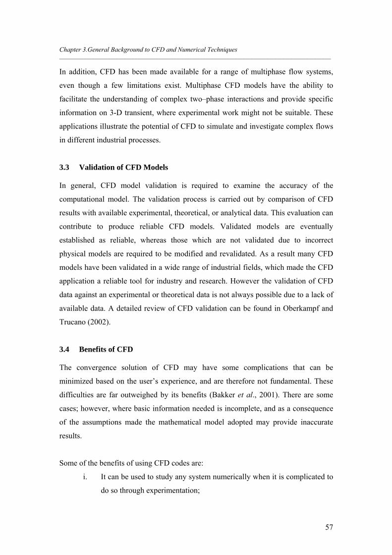
Chapter 3.General Background to CFD and Numerical Techniques _______________________________________________________________________________________________________
57
In addition, CFD has been made available for a range of multiphase flow systems,
even though a few limitations exist. Multiphase CFD models have the ability to
facilitate the understanding of complex two–phase interactions and provide specific
information on 3-D transient, where experimental work might not be suitable. These
applications illustrate the potential of CFD to simulate and investigate complex flows
in different industrial processes.
3.3 Validation of CFD Models
In general, CFD model validation is required to examine the accuracy of the
computational model. The validation process is carried out by comparison of CFD
results with available experimental, theoretical, or analytical data. This evaluation can
contribute to produce reliable CFD models. Validated models are eventually
established as reliable, whereas those which are not validated due to incorrect
physical models are required to be modified and revalidated. As a result many CFD
models have been validated in a wide range of industrial fields, which made the CFD
application a reliable tool for industry and research. However the validation of CFD
data against an experimental or theoretical data is not always possible due to a lack of
available data. A detailed review of CFD validation can be found in Oberkampf and
Trucano (2002).
3.4 Benefits of CFD
The convergence solution of CFD may have some complications that can be
minimized based on the user’s experience, and are therefore not fundamental. These
difficulties are far outweighed by its benefits (Bakker et al., 2001). There are some
cases; however, where basic information needed is incomplete, and as a consequence
of the assumptions made the mathematical model adopted may provide inaccurate
results.
Some of the benefits of using CFD codes are:
i. It can be used to study any system numerically when it is complicated to
do so through experimentation;
Chapter 3.General Background to CFD and Numerical Techniques _______________________________________________________________________________________________________
58
ii. CFD is able to provide different kinds of information which can be
difficult to obtain through experimentation due to the limitation of
equipment or technique;
iii. The complex physical interactions that take place in a flow condition can
be modeled simultaneously since no limiting assumptions are usually
required.
iv. CFD also enables the visualization of the flow behaviour of a system,
and it is commonly used in industry as a flow visualisation tool (Gaylard,
2001).
3.5 CFD Analysis Procedure
To employ CFD in process system investigations, the following information is
required:
i. A grid of points is used to store the variables calculated by CFD;
ii. Boundary conditions are needed for defining the conditions at the flow
domain boundaries and to allow the boundary values of all variables to be
estimated;
iii. Fluid properties are required to be specified, such as viscosity and density;
iv. Flow models describe the various characteristics of the flow, for instance
mass, heat transfer, turbulence, and multiphase models;
v. Initial conditions are used to give the initial state of the flow for a transient
simulation or an initial guess of the solution variables in a steady state
simulation;
vi. Solver control parameters are necessary to manage the behaviour of the
numerical solution process; and
vii. Analysis of the results is done to verify that the solution is satisfactory
against reliable data or correlation and to estimate the flow data required.
The entire CFD analysis structure can be classified into six steps as follows.
Chapter 3.General Background to CFD and Numerical Techniques _______________________________________________________________________________________________________
59
3.5.1 Initial Thinking
One of the fundamentals of this stage is to know and understand the problem before
simulation in order to select the correct physical model that describes the case. This
stage also requires some data which are necessary for the simulation, such as
geometry details, fluid properties, flow specifications, and boundary and initial
conditions.
3.5.2 Geometry Construction
The flow domain geometry is created by special software for drawing called Gambit.
First of all, 2-D sketches are typically drawn and then 3-D tools are employed to
generate the full geometry, which gives more accurate information about the problem
such as that taking place in reality.
3.5.3 Mesh Generation
The flow domain space is subdivided into sufficiently small discrete cells. These cells
are allocated to determine the positions of the flow variables which are to be
computed and stored up. Usually variable gradients are not accurately calculated on a
coarse mesh but on a fine one. Therefore, a fine mesh is very significant in regions
where the flow variables are expected to have large variations. More computational
power and time are required with a fine mesh. The optimization of mesh size is
considered as a critical test that examines the simulation results with respect to mesh
refinement.
3.5.4 Flow Specification
This step consists of defining the flow models, fluid physical properties, flow
boundary conditions, and initial flow conditions, as found in the initial thinking step.
3.5.5 Calculation of the Numerical Solution
When the simulation set up is done using all the required information, iterative
calculations are carried out by the CFD to reach a solution to the numerical equations
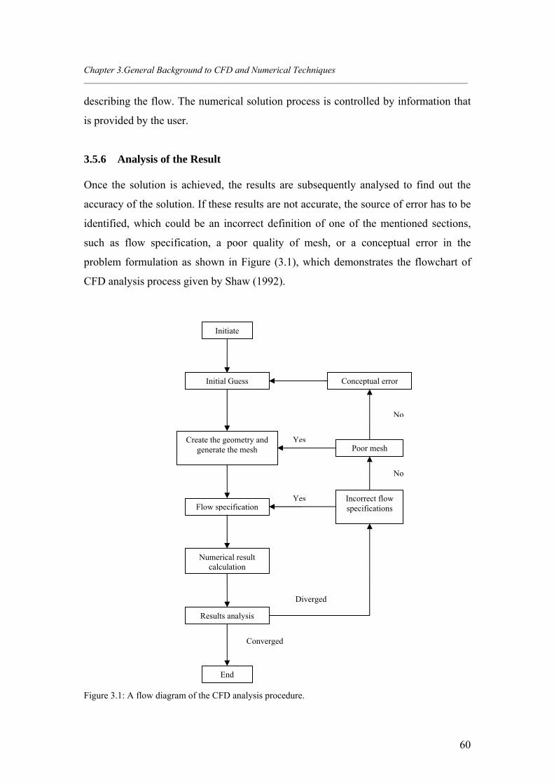
Chapter 3.General Background to CFD and Numerical Techniques _______________________________________________________________________________________________________
60
describing the flow. The numerical solution process is controlled by information that
is provided by the user.
3.5.6 Analysis of the Result
Once the solution is achieved, the results are subsequently analysed to find out the
accuracy of the solution. If these results are not accurate, the source of error has to be
identified, which could be an incorrect definition of one of the mentioned sections,
such as flow specification, a poor quality of mesh, or a conceptual error in the
problem formulation as shown in Figure (3.1), which demonstrates the flowchart of
CFD analysis process given by Shaw (1992).
Figure 3.1: A flow diagram of the CFD analysis procedure.
Initiate
Initial Guess
Create the geometry and generate the mesh
Flow specification
Numerical result calculation
Results analysis
End
Incorrect flow specifications
Poor mesh
Conceptual error
Yes
No
Yes
No
Converged
Diverged
Chapter 3.General Background to CFD and Numerical Techniques _______________________________________________________________________________________________________
61
3.6 Existing Commercial CFD Codes
In the last two decades, CFD has received interest from industry. This has led to the
development of a variety of CFD codes that are available commercially, for instance
CFX, FLUENT, PHOENICS, and STAR-CD. The benefit of these codes is that they
can deal with many complex areas of fluid flow in industrial applications. Generally,
the CFD package is made of three main components, which are:
a. A pre-processor
b. A solver
c. A post-processor
The first step is a pre-processor, which is considered the most important one because
it involves the creation of geometry and mesh. After that the flow model, fluid
properties and control parameters of the solver are specified, and then the boundary
and initial conditions are applied. The second step is a solver that is used to discretise
and solve the numerical transport equations based on the specified data. The final step
is a post-processor, in which the output results of the simulation can be visualised and
analysed.
3.7 Numerical Techniques
The governing equations are typically presented by partial differential equations
(PDEs), such as Navier–Stokes equations. Such equations can not be solved directly
using digital computers that are able to identify and operate with numerical data.
However, the PDEs have to be converted into numerical equations that include only
numbers and no derivates. This process of transferring the PDEs to a numerical
analogue is called Numerical Discretisation, where various approaches are used for
solving, including finite difference method, finite element method, and finite volume
method.
The method of Finite–difference is derived based on the use of the Taylor series to
change the partial differential equations into derivatives of dependent variables as
there are differences among the variable values at various points in space and time.
Chapter 3.General Background to CFD and Numerical Techniques _______________________________________________________________________________________________________
62
Linear algebraic equations are produced as a result of PDEs being transferred so that
they can be solved by one of the elimination approaches.
In the finite element method, the domain is separated into a finite number of small
elements or sub–domains. A simple variant of the dependent variables is assumed
over individual element, where this variable variant is computed based on the values
of the variable at the element nodes. The obtained equations for individual elements
are then placed in a matrix and boundary conditions are applied to solve the equations
in the matrix.
The finite volume method is that most employed for numerical discretisation. It is a
similar mode of application to the finite different method, while some of its
implementations are driven on characteristics based on the finite element approach.
This method takes into account the discretisation of the spatial domain into finite
control volumes. A control volume usually covers many mesh elements that can be
divided into sectors which belong to a different mesh element. The differential
governing equations are integrated over individual control volumes. The result of this
integration ensures the accurate conservation of related properties in individual finite
volumes. Each integral term is transformed to a discrete term that results into
discretised equations at the nodal, or centroids points of the control volumes. This
method is similar to the finite difference method where the numerical equations at a
particular point are derived from the values at neighbouring points.
3.8 CFD Modelling Approaches for Multiphase
The modelling of multi–phase flow is considered an enormous topic and includes a
wide range of industrial processes. Multi–fluid flow has been given special treatment
in oil and gas engineering due to its importance, and is significant in the current study
of two–phase flows in horizontal pipelines. This section revises the multi–phase
modelling aspects of dispersed and stratified flow, which are very common in low
liquid loading two–phase flow. In reality most of the fluids flow as a turbulent due to
the nature of the operating conditions. This section also discusses various turbulence
modelling features in two–phase flow systems. Particular attention is given to the
Chapter 3.General Background to CFD and Numerical Techniques _______________________________________________________________________________________________________
63
treatment of interface forces that play an important role in the prediction of system
parameters.
It is important to understand the need for modelling flow fields and turbulence in
order to resolve them directly. A special technique which provides for an exact
computation of the instantaneous flow fields and their turbulent fluctuations without
resorting to any kind of modelling is discussed. This method has some limitations that
are emphasized and, therefore, the requirement for modelling is demonstrated.
3.8.1 Dispersed Multi–fluid Flow Modelling
There are four recognized methods to modelling dispersed multi–phase flows
(Ranade, 2002):
1. Volume of Fluid (the Eulerian framework for both phases with interface
forces reformulation based on a volumetric basis).
2. Eulerian-Lagrangian (the continuous and dispersed phases are treated in the
framework of Eulerian and Lagrangian respectively).
3. Eulerian-Eulerian (both phases are treated within the Eulerian framework, not
including explicitly for the interface between phases), and
4. Mixture (it treats both phases as continuous and dispersed as a one mixture
phase).
3.8.1.1 Volume of Fluid (VOF) Approach
The volume of fluid method tracks the motion of a distinct phase in each cell through
the domain. In the VOF model, a single set of conservation equations is shared by the
two–phase using mixture properties, when both phases share the same control
volume. In addition, if the control volume is occupied by one of the phases, its related
properties are utilized. The benefit of this is to avoid any unexpected changes in the
physical properties of the fluid through a thin interface.
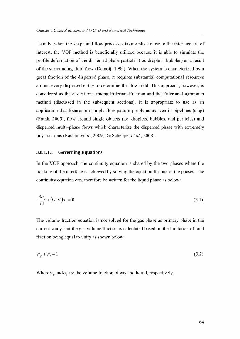
Chapter 3.General Background to CFD and Numerical Techniques _______________________________________________________________________________________________________
64
Usually, when the shape and flow processes taking place close to the interface are of
interest, the VOF method is beneficially utilized because it is able to simulate the
profile deformation of the dispersed phase particles (i.e. droplets, bubbles) as a result
of the surrounding fluid flow (Delnoij, 1999). When the system is characterized by a
great fraction of the dispersed phase, it requires substantial computational resources
around every dispersed entity to determine the flow field. This approach, however, is
considered as the easiest one among Eulerian–Eulerian and the Eulerian–Lagrangian
method (discussed in the subsequent sections). It is appropriate to use as an
application that focuses on simple flow pattern problems as seen in pipelines (slug)
(Frank, 2005), flow around single objects (i.e. droplets, bubbles, and particles) and
dispersed multi–phase flows which characterize the dispersed phase with extremely
tiny fractions (Rashmi et al., 2009, De Schepper et al., 2008).
3.8.1.1.1 Governing Equations
In the VOF approach, the continuity equation is shared by the two phases where the
tracking of the interface is achieved by solving the equation for one of the phases. The
continuity equation can, therefore be written for the liquid phase as below:
0.
lil U
t
(3.1)
The volume fraction equation is not solved for the gas phase as primary phase in the
current study, but the gas volume fraction is calculated based on the limitation of total
fraction being equal to unity as shown below:
1 lg (3.2)
Where g and l are the volume fraction of gas and liquid, respectively.
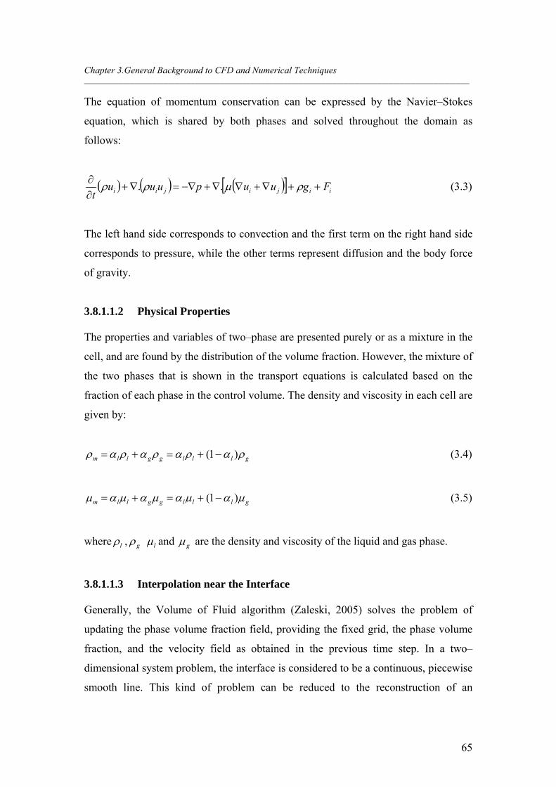
Chapter 3.General Background to CFD and Numerical Techniques _______________________________________________________________________________________________________
65
The equation of momentum conservation can be expressed by the Navier–Stokes
equation, which is shared by both phases and solved throughout the domain as
follows:
iijijii Fguupuuut
.. (3.3)
The left hand side corresponds to convection and the first term on the right hand side
corresponds to pressure, while the other terms represent diffusion and the body force
of gravity.
3.8.1.1.2 Physical Properties
The properties and variables of two–phase are presented purely or as a mixture in the
cell, and are found by the distribution of the volume fraction. However, the mixture of
the two phases that is shown in the transport equations is calculated based on the
fraction of each phase in the control volume. The density and viscosity in each cell are
given by:
glllggllm )1( (3.4)
glllggllm )1( (3.5)
where l , g l and g are the density and viscosity of the liquid and gas phase.
3.8.1.1.3 Interpolation near the Interface
Generally, the Volume of Fluid algorithm (Zaleski, 2005) solves the problem of
updating the phase volume fraction field, providing the fixed grid, the phase volume
fraction, and the velocity field as obtained in the previous time step. In a two–
dimensional system problem, the interface is considered to be a continuous, piecewise
smooth line. This kind of problem can be reduced to the reconstruction of an
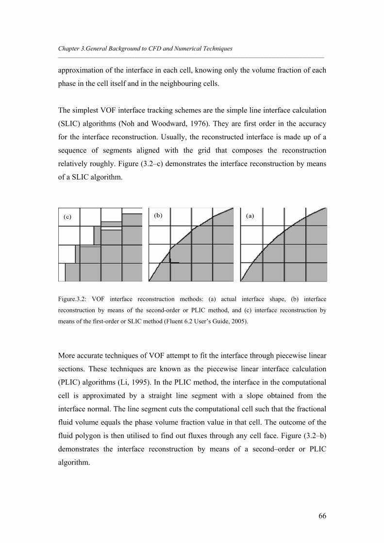
Chapter 3.General Background to CFD and Numerical Techniques _______________________________________________________________________________________________________
66
approximation of the interface in each cell, knowing only the volume fraction of each
phase in the cell itself and in the neighbouring cells.
The simplest VOF interface tracking schemes are the simple line interface calculation
(SLIC) algorithms (Noh and Woodward, 1976). They are first order in the accuracy
for the interface reconstruction. Usually, the reconstructed interface is made up of a
sequence of segments aligned with the grid that composes the reconstruction
relatively roughly. Figure (3.2–c) demonstrates the interface reconstruction by means
of a SLIC algorithm.
Figure.3.2: VOF interface reconstruction methods: (a) actual interface shape, (b) interface
reconstruction by means of the second-order or PLIC method, and (c) interface reconstruction by
means of the first-order or SLIC method (Fluent 6.2 User’s Guide, 2005).
More accurate techniques of VOF attempt to fit the interface through piecewise linear
sections. These techniques are known as the piecewise linear interface calculation
(PLIC) algorithms (Li, 1995). In the PLIC method, the interface in the computational
cell is approximated by a straight line segment with a slope obtained from the
interface normal. The line segment cuts the computational cell such that the fractional
fluid volume equals the phase volume fraction value in that cell. The outcome of the
fluid polygon is then utilised to find out fluxes through any cell face. Figure (3.2–b)
demonstrates the interface reconstruction by means of a second–order or PLIC
algorithm.
Chapter 3.General Background to CFD and Numerical Techniques _______________________________________________________________________________________________________
67
One of the significant simplifying characteristics of VOF/PLIC algorithms is that it
does not attempt to reconstruct the interface as a continuous chain of segments.
Therefore, the alternating chain with small discontinuities is retained. When the
curvature is small, the scheme will be more accurate. A VOF/PLIC algorithm
involves a two–step that is both a reconstruction and a propagation step. In the
reconstruction step, a linear interface that separates the computational cell into two
sections containing an appropriate area of each of the two–phase is constructed. The
orientation of the segment is found through the calculation of the unit normal vector
to the segment.
Many algorithms have been developed for the calculation of the unit normal vector
(Puckett, 1991). This unit normal vector, together with the value of phase volume
fraction in the cell, uniquely establishes the linear interface in the cell. The second
step of the VOF algorithm is propagation (Puckett, 1997). Once the interface has been
constructed, the interface motion caused by the velocity field must be modeled with a
suitable advection algorithm.
In the existing CFD code, this scheme is the most accurate one and it is applicable for
general unstructured meshes as used here. As typical for the PLIC method, this
interpolation scheme assumes that the interface between two fluids has a linear slope
within each cell and this linear shape is used for the calculation of the advection of the
fluid through the cell interfaces.
The first step in this reconstruction scheme consists of the calculation of the position
of the linear interface relative to the center of each partially filled cell, based on
information concerning the volume fraction and its derivatives in the cell. The second
step is the calculation of the advecting amount of fluid through each interface using
the computed linear interface representation and information about the normal and
tangential velocity distribution at the interface. In the third step, the volume fraction
in each cell is determined using the balance of fluid mass fluxes calculated in the
previous time step.
Chapter 3.General Background to CFD and Numerical Techniques _______________________________________________________________________________________________________
68
The Compressive Interface Capturing Scheme for Arbitrary Meshes (CICSAM) is
another method to improve the accuracy of the interface in the VOF approach and is
based on Ubbink’s research (1997). This method is suitable for flows with high ratios
of viscosity differences between the phases. It is implemented in FLUENT as an
explicit approach and provides an advantage of producing a sharp interface that is
similar to that produced by a geometric reconstruction method. During all simulations
in the current work in Chapter 4, the CICSAM interface reconstruction approach has
been utilized for interpolation in a cell.
3.8.1.2 Eulerian–Lagrangian (E–L) Approach
In the Eulerian–Lagrangian method, the fluid phase is considered as a continuum.
This is solved by time averaged of Navier–Stokes equations in the same way as it
solved for a single phase system, whilst the dispersed phase is solved by the equation
of motion for each dispersed phase entity where the explicit motion of the interface is
not modeled in this approach.
This method is able to capture the dispersed fluid dynamics accurately. Particle–level
processes (e.g. chemical reactions, heat and mass transfer effects etc) can be
simulated in sufficient manner and detailed and accounts for interaction between
particles and size distribution. However, a large number of particles are required in
turbulent flow simulation in order to achieve a significant average. Subsequently, as
the number of dispersed droplets, bubbles or particles increases, the computational
cost increases proportionally, and as result this approach is limited to simulating two–
phase flow with low fraction of less than 10% of dispersed flow (Domgin et al., 1997;
Jaworski and Pianko–Oprych, 2002).
3.8.1.2.1 Governing Equations
This approach is used for modelling a hydrodynamic or multiphase flow, where the
particle models are integrated with an Eulerian model for the continuous fluid in order
to simulate the disperse fluid. The fluid phase movement is attained by calculating the
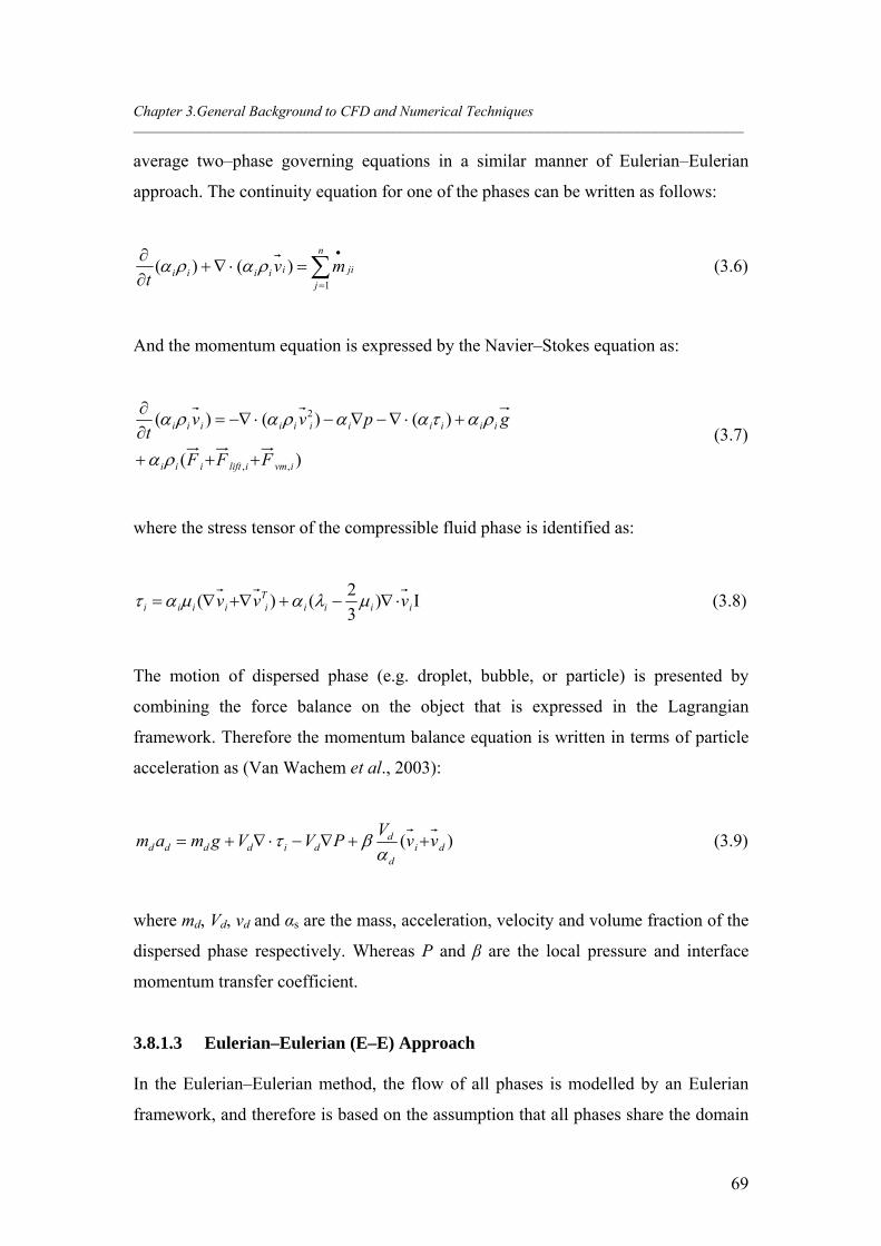
Chapter 3.General Background to CFD and Numerical Techniques _______________________________________________________________________________________________________
69
average two–phase governing equations in a similar manner of Eulerian–Eulerian
approach. The continuity equation for one of the phases can be written as follows:
n
j
jiiiiii mvt 1
)()( (3.6)
And the momentum equation is expressed by the Navier–Stokes equation as:
)(
)()()(
,,
2
ivmiliftiii
iiiiiiiiiii
FFF
gpvvt
(3.7)
where the stress tensor of the compressible fluid phase is identified as:
iiiiTiiiii vvv )
3
2()( (3.8)
The motion of dispersed phase (e.g. droplet, bubble, or particle) is presented by
combining the force balance on the object that is expressed in the Lagrangian
framework. Therefore the momentum balance equation is written in terms of particle
acceleration as (Van Wachem et al., 2003):
)( did
ddidddd vv
VPVVgmam
(3.9)
where md, Vd, vd and αs are the mass, acceleration, velocity and volume fraction of the
dispersed phase respectively. Whereas P and β are the local pressure and interface
momentum transfer coefficient.
3.8.1.3 Eulerian–Eulerian (E–E) Approach
In the Eulerian–Eulerian method, the flow of all phases is modelled by an Eulerian
framework, and therefore is based on the assumption that all phases share the domain
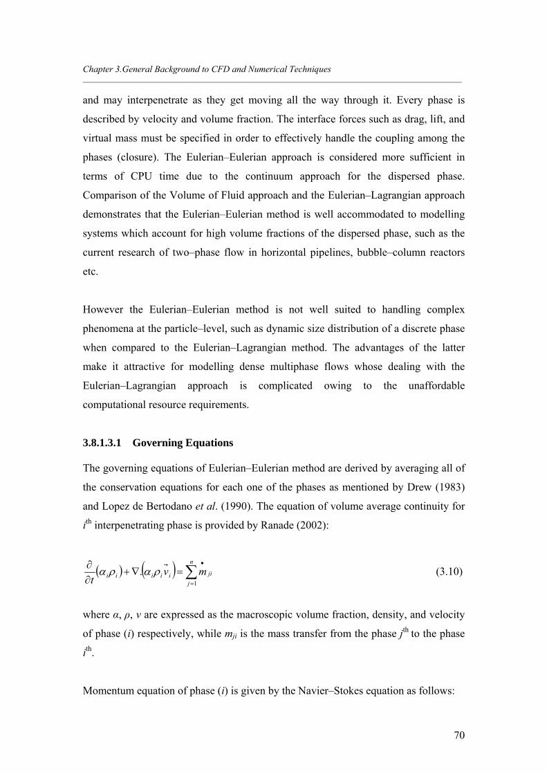
Chapter 3.General Background to CFD and Numerical Techniques _______________________________________________________________________________________________________
70
and may interpenetrate as they get moving all the way through it. Every phase is
described by velocity and volume fraction. The interface forces such as drag, lift, and
virtual mass must be specified in order to effectively handle the coupling among the
phases (closure). The Eulerian–Eulerian approach is considered more sufficient in
terms of CPU time due to the continuum approach for the dispersed phase.
Comparison of the Volume of Fluid approach and the Eulerian–Lagrangian approach
demonstrates that the Eulerian–Eulerian method is well accommodated to modelling
systems which account for high volume fractions of the dispersed phase, such as the
current research of two–phase flow in horizontal pipelines, bubble–column reactors
etc.
However the Eulerian–Eulerian method is not well suited to handling complex
phenomena at the particle–level, such as dynamic size distribution of a discrete phase
when compared to the Eulerian–Lagrangian method. The advantages of the latter
make it attractive for modelling dense multiphase flows whose dealing with the
Eulerian–Lagrangian approach is complicated owing to the unaffordable
computational resource requirements.
3.8.1.3.1 Governing Equations
The governing equations of Eulerian–Eulerian method are derived by averaging all of
the conservation equations for each one of the phases as mentioned by Drew (1983)
and Lopez de Bertodano et al. (1990). The equation of volume average continuity for
ith interpenetrating phase is provided by Ranade (2002):
n
j
jiiiiii mvt 1
. (3.10)
where α, ρ, v are expressed as the macroscopic volume fraction, density, and velocity
of phase (i) respectively, while mji is the mass transfer from the phase jth to the phase
ith.
Momentum equation of phase (i) is given by the Navier–Stokes equation as follows:
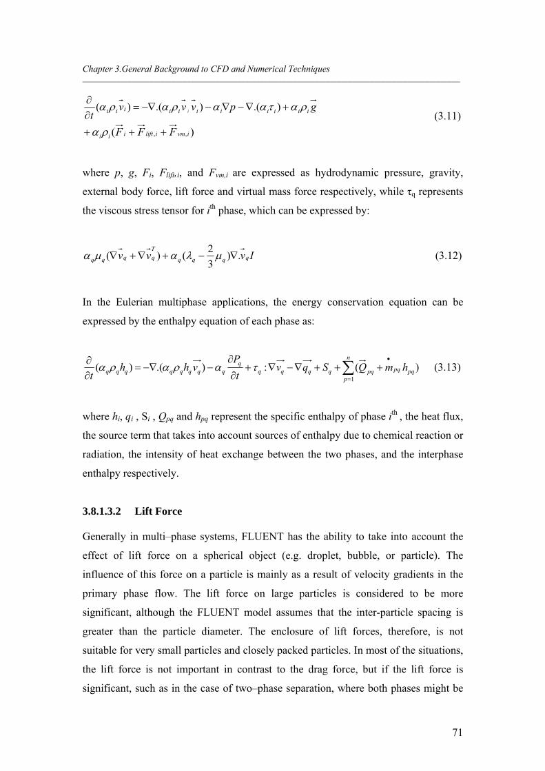
Chapter 3.General Background to CFD and Numerical Techniques _______________________________________________________________________________________________________
71
)(
).().()(
,, ivmiliftiii
iiiiiiiiiii
FFF
gpvvvt
i
(3.11)
where p, g, Fi, Flift,i, and Fvm,i are expressed as hydrodynamic pressure, gravity,
external body force, lift force and virtual mass force respectively, while τq represents
the viscous stress tensor for ith phase, which can be expressed by:
Ivvv qqqq
T
qqqq .)3
2()( (3.12)
In the Eulerian multiphase applications, the energy conservation equation can be
expressed by the enthalpy equation of each phase as:
n
ppqpqpqqqqq
qqqqqqqqq hmQSqv
t
Pvhh
t 1
)(:).()( (3.13)
where hi, qi , Si , Qpq and hpq represent the specific enthalpy of phase ith , the heat flux,
the source term that takes into account sources of enthalpy due to chemical reaction or
radiation, the intensity of heat exchange between the two phases, and the interphase
enthalpy respectively.
3.8.1.3.2 Lift Force
Generally in multi–phase systems, FLUENT has the ability to take into account the
effect of lift force on a spherical object (e.g. droplet, bubble, or particle). The
influence of this force on a particle is mainly as a result of velocity gradients in the
primary phase flow. The lift force on large particles is considered to be more
significant, although the FLUENT model assumes that the inter-particle spacing is
greater than the particle diameter. The enclosure of lift forces, therefore, is not
suitable for very small particles and closely packed particles. In most of the situations,
the lift force is not important in contrast to the drag force, but if the lift force is
significant, such as in the case of two–phase separation, where both phases might be
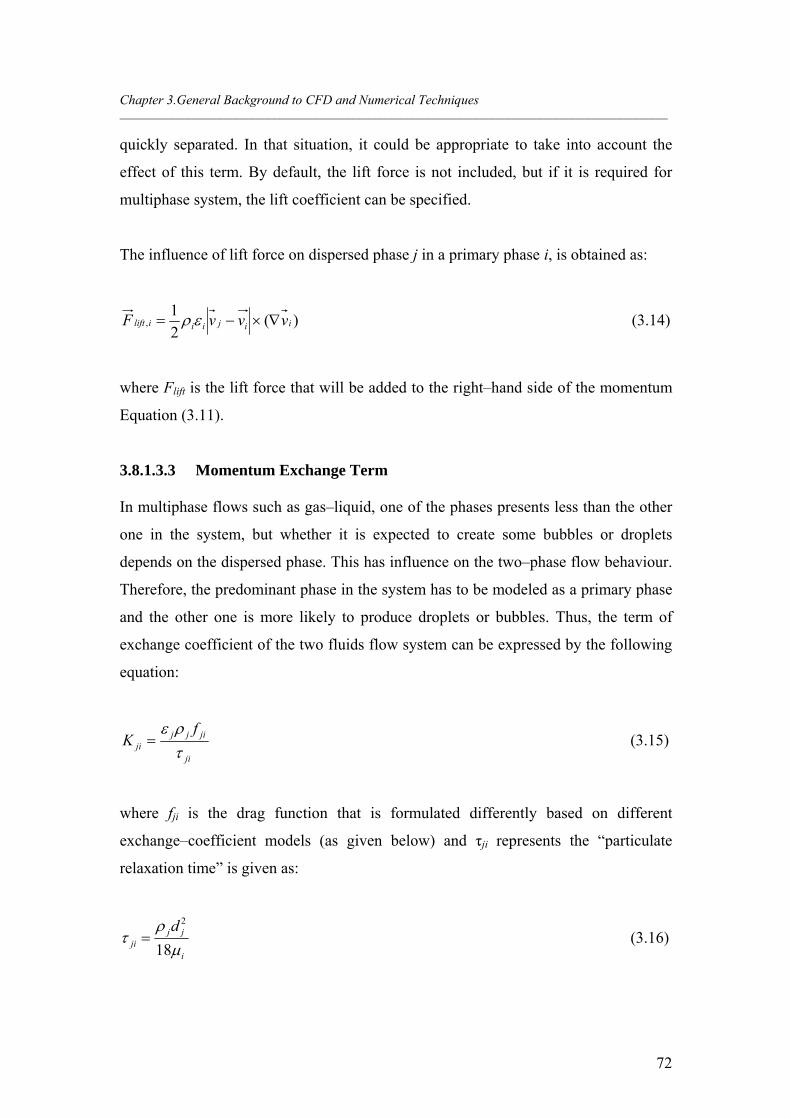
Chapter 3.General Background to CFD and Numerical Techniques _______________________________________________________________________________________________________
72
quickly separated. In that situation, it could be appropriate to take into account the
effect of this term. By default, the lift force is not included, but if it is required for
multiphase system, the lift coefficient can be specified.
The influence of lift force on dispersed phase j in a primary phase i, is obtained as:
)(2
1, iijiiilift vvvF (3.14)
where Flift is the lift force that will be added to the right–hand side of the momentum
Equation (3.11).
3.8.1.3.3 Momentum Exchange Term
In multiphase flows such as gas–liquid, one of the phases presents less than the other
one in the system, but whether it is expected to create some bubbles or droplets
depends on the dispersed phase. This has influence on the two–phase flow behaviour.
Therefore, the predominant phase in the system has to be modeled as a primary phase
and the other one is more likely to produce droplets or bubbles. Thus, the term of
exchange coefficient of the two fluids flow system can be expressed by the following
equation:
ji
jijjji
fK
(3.15)
where fji is the drag function that is formulated differently based on different
exchange–coefficient models (as given below) and τji represents the “particulate
relaxation time” is given as:
i
jjji
d
18
2
(3.16)
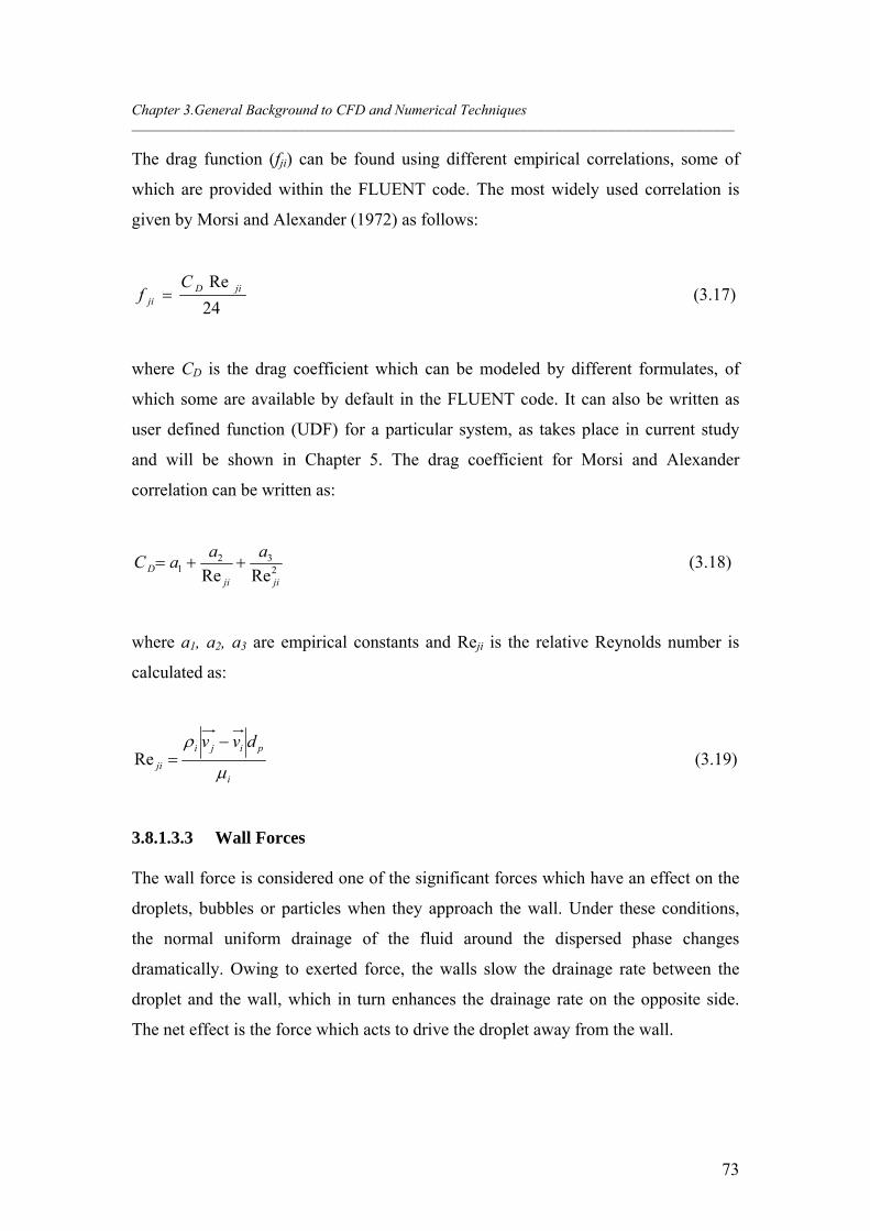
Chapter 3.General Background to CFD and Numerical Techniques _______________________________________________________________________________________________________
73
The drag function (fji) can be found using different empirical correlations, some of
which are provided within the FLUENT code. The most widely used correlation is
given by Morsi and Alexander (1972) as follows:
24
Re jiDji
Cf (3.17)
where CD is the drag coefficient which can be modeled by different formulates, of
which some are available by default in the FLUENT code. It can also be written as
user defined function (UDF) for a particular system, as takes place in current study
and will be shown in Chapter 5. The drag coefficient for Morsi and Alexander
correlation can be written as:
232
1 ReRe jijiD
aaaC (3.18)
where a1, a2, a3 are empirical constants and Reji is the relative Reynolds number is
calculated as:
i
piji
ji
dvv
Re (3.19)
3.8.1.3.3 Wall Forces
The wall force is considered one of the significant forces which have an effect on the
droplets, bubbles or particles when they approach the wall. Under these conditions,
the normal uniform drainage of the fluid around the dispersed phase changes
dramatically. Owing to exerted force, the walls slow the drainage rate between the
droplet and the wall, which in turn enhances the drainage rate on the opposite side.
The net effect is the force which acts to drive the droplet away from the wall.
Chapter 3.General Background to CFD and Numerical Techniques _______________________________________________________________________________________________________
74
3.8.1.4 Mixture
The mixture model is one of the simplified multi–fluid approaches, which can be
utilized to simulate two phases of different or same velocities, but assumes the local
equilibrium within small spatial length scales (FLUENT, 2005). As a result, the
accelerating entities of dispersed fluid reach the terminal velocity after travelling a
distance in which the length scale of the system is become greater (Chen et al., 2005).
The relative velocity among the fluids is described by using an algebraic equation,
which is based on the local equilibrium assumption (Hossain et al., 2003, and Chen et
al., 2005). In contrast to the Volume of Fluid (VOF) model, the two phases into the
mixture approach are permitted to interpenetrating, where the dispersed phase is
characterised by a volume fraction equation. Each dispersed phase has its individual
transport equation, which allows for the slip velocity between the phases (dispersed
and continuous).
Based on the mixture model theory, it treats both phases of continuous and dispersed
as a single phase. This is considered as a mixture phase in which physical properties,
such as density and viscosity of the mixture, are found based on each phase fraction.
These properties are employed in the governing equation. Furthermore, the
homogeneous multiphase flows can be simulated by the mixture model with very
strong coupling between the phases, which flow nearly with the same velocity. The
computational time of this model is much lower than other multiphase models which
have been discussed before, because it solves the minimum number of equations.
Nevertheless, there is a strong compromise in the level of flow information it can
present when compared with the inclusive Eulerian–Eulerian method. In addition,
none of drag interphase forces such as the lift and virtual mass forces are calculated
into the mixture model. The mixture model can be used in many industrial
applications, for instance sedimentation, bubbly flows where the dispersed phase
fraction remains low and particle–laden flows with low loading.
The mixture model also solves most of the equations for the mixture, such as the
continuity, momentum, and energy equation. The volume fraction equation is solved
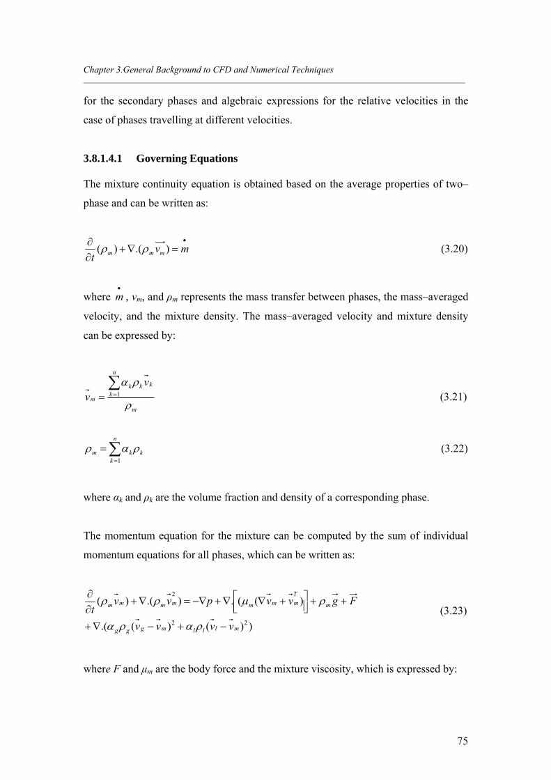
Chapter 3.General Background to CFD and Numerical Techniques _______________________________________________________________________________________________________
75
for the secondary phases and algebraic expressions for the relative velocities in the
case of phases travelling at different velocities.
3.8.1.4.1 Governing Equations
The mixture continuity equation is obtained based on the average properties of two–
phase and can be written as:
mvt mmm ).()( (3.20)
where
m , vm, and ρm represents the mass transfer between phases, the mass–averaged
velocity, and the mixture density. The mass–averaged velocity and mixture density
can be expressed by:
m
n
k
kkk
m
vv
1 (3.21)
n
kkkm
1
(3.22)
where αk and ρk are the volume fraction and density of a corresponding phase.
The momentum equation for the mixture can be computed by the sum of individual
momentum equations for all phases, which can be written as:
))()(.(
)((.).()(
22
2
mlllmggg
m
T
mmmmmmm
vvvv
Fgvvpvvt
(3.23)
where F and μm are the body force and the mixture viscosity, which is expressed by:
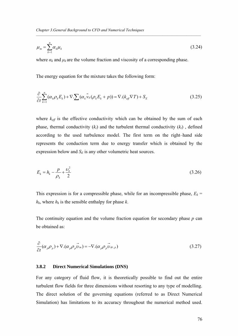
Chapter 3.General Background to CFD and Numerical Techniques _______________________________________________________________________________________________________
76
n
kkkm
1
(3.24)
where αk and μk are the volume fraction and viscosity of a corresponding phase.
The energy equation for the mixture takes the following form:
Eeffkkkkkk
n
kk STkpEvE
t
).())((.)(1
(3.25)
where keff is the effective conductivity which can be obtained by the sum of each
phase, thermal conductivity (ki) and the turbulent thermal conductivity (kt) , defined
according to the used turbulence model. The first term on the right–hand side
represents the conduction term due to energy transfer which is obtained by the
expression below and SE is any other volumetric heat sources.
2
2k
kkk
phE
(3.26)
This expression is for a compressible phase, while for an incompressible phase, Ek =
hk, where hk is the sensible enthalpy for phase k.
The continuity equation and the volume fraction equation for secondary phase p can
be obtained as:
).().()( , pdrppmppppt
(3.27)
3.8.2 Direct Numerical Simulations (DNS)
For any category of fluid flow, it is theoretically possible to find out the entire
turbulent flow fields for three dimensions without resorting to any type of modelling.
The direct solution of the governing equations (referred to as Direct Numerical
Simulation) has limitations to its accuracy throughout the numerical method used.
Chapter 3.General Background to CFD and Numerical Techniques _______________________________________________________________________________________________________
77
This method produces a lot of data including the time history of all flow variables at
each point in the domain. The characteristic of direct numerical simulation (DNS)
therefore is a beneficial way to study and understand the fundamentals of fluid flow
dynamics and turbulence phenomena, and as a result this assists in the evaluation and
development of existing models.
The DNS method however is not sufficient for practical engineering problems, mainly
owing to the excessive mesh sizes that are required to resolve all scales of motion in
the three spatial dimensions (FLUENT, 2005). Furthermore, the requirement of initial
and boundary conditions is considered as one of the most significant and difficult
stages in using the concept of DNS (Ranade, 2002). Further to the complexity of this
approach, the simulation would have to be a transient one with very small time steps.
Consequently, a computational power is needed to solve the highly dispersed phase
fraction, and usually turbulent and multi–phase flows are beyond the abilities of even
modern computers.
3.8.3 Treatment of Turbulence in Multi–fluid Flows
Multi–fluid dispersions detected in Chemical Process Industries (CPI) are basically
turbulent in nature and are thus classified based on velocity fields fluctuation. These
variations combine transported quantities such as energy and momentum, as well as
species concentration, and cause them to fluctuate as well. As these fluctuations can
be of small scale and high frequency, they become extremely expensive to be
simulated directly by DNS in terms of computational process time, as discussed in
Section 3.8.2. As an alternative, the instantaneous governing equations can be time–
averaged, ensemble–averaged, or otherwise controlled to remove the small scales of
Large Eddy simulation (LES), leading to reformulate a set of equations, which then be
developed and become computationally less expensive to solve. Nevertheless, the
modified equations have additional unidentified variables, and turbulence models are
required in order to find these variables in terms of known quantities (closure).
Chapter 3.General Background to CFD and Numerical Techniques _______________________________________________________________________________________________________
78
3.8.3.1 Large Eddy Simulations (LES)
Large Eddy Simulations (LES) are based on the assumption that the relevant scales in
turbulent flows can be divided into large and small–scale (also referred to as sub–
grid) components as shown in Figure (3.3). In this approach, it is implicitly assumed
that such separation does not considerably affect the evolution of large–scale
turbulent motions. The large–scale motions are generally much more energetic than
the small–scale motions, and as a result of that they contribute more to the transport of
conserved quantities. However, LES aims to simulate these large–scale motions much
more specifically than small–scale motions, which are considered to be more general
in character and hence more easily to be modeled.
The requirements of mesh resolution and time–step sizes are less restrictive in
contrast with the DNS approach. Even though LES have many advantages, they still
have some problems, similar to the shortcomings of DNS such as difficulties in
specifying boundary conditions and generating a huge amount of information which is
not useful for practical purposes (Bakker and Oshinowo, 2004).
The restricted ability (due to computational limitations) of using the DNS or LES
methods to flows of practical interest in CPI conducts the use of computationally
more tractable turbulence models based on the Reynolds Averaged Navier Stokes
(RANS) equation (Prasad et al., 1998; Bakker and Oshinowo, 2004), which is
explained in the next section. It should be noted that the latest advances in modelling
have resulted in a hybrid approach that combines RANS modelling with LES, known
as Detached Eddy Simulation (DES). Basically, DES reduces to RANS in regions
which are close to the walls, and changes to LES in regions away from the walls
(Constantinescu and Squires, 2003).
The outcome of this leads to a decrease in the computational effort significantly,
while providing more accurate flow features when compared to RANS.
Chapter 3.General Background to CFD and Numerical Techniques _______________________________________________________________________________________________________
79
Figure 3.3: Schematic representation of scales in turbulent flows (adapted from Ferziger and Peric,
1995).
3.8.3.2 Turbulence Models Based on RANS
In this approach of RANS, the instantaneous value of any flow variable () is
decomposed into a mean ( ) and a fluctuating component ( ):
(3.28)
where, , and are the Instantaneous value, Time averaged mean, and Fluctuating
component, respectively.
The mean value can be found by averaging over an appropriate time interval, where
the Reynolds averaging obeys the following properties:
and 0 (3.29)
where the over bar describes time averaging. Equation (3.28) is substituted in the
basic governing equations for the flow variable () (e.g. velocity of a phase) followed
by time averaging, subject to the conditions listed in Equation (3.29) in order to yield
governing equations for the mean quantities. When simplified the equation is led to a
new averaged equation featuring an extra term which takes into account the turbulent
transport of ‘’. As the fluctuation of time averaged quantities takes place at much
Chapter 3.General Background to CFD and Numerical Techniques _______________________________________________________________________________________________________
80
larger scales, resolving the smaller spatial and temporal scales is not needed in the
RANS–based approach.
The variation of fluid velocity with time is shown in Figure (3.4) and also
demonstrates a comparison between the RANS based approach with the DNS and
LES approaches.
Figure 3.4: A comparison of DNS, LES and RANS (Ranade, 2002).
The averaging of RANS approach requires considerably less computational power
compared to the LES or DNS methods. However, time averaging the basic governing
equations results in the creation of new terms which lead to a closure difficulty. These
new expressions might be integrated as apparent stress gradients and heat/mass fluxes
associated with turbulent motion (Ranade, 2002). The governing equations for these
new expressions can be derived theoretically. On the other hand, the obtained
equations would also have more unknown expressions. Therefore, it becomes very
important to establish a turbulence model, which relates these unidentified terms to
known ones in order to complete the set of governing equations. During the last three
decades, several turbulence models have been developed and utilized in simulations
that have confirmed different degrees of achievement. In the next section, a
comprehensive description of two–equation models will be given, such as standard k–
Chapter 3.General Background to CFD and Numerical Techniques _______________________________________________________________________________________________________
81
ε, Renormalization Group (RNG) k–ε, and k–ω. That discussion will focus on the
advantages, limitations and the range of applicability of each model.
3.8.3.2.1 k−ε Model
Generally, the k–ε model is the most utilized turbulence model to simulate turbulence
eddies. The k–ε turbulence model is described by a semi–empirical model, which is
based on model transport equations for the turbulence kinetic energy (k) and its
dissipation rate (ε). The transport equation for turbulence kinetic energy (k) is
obtained from the explicit equation, whereas the equation of dissipation rate (ε) is
derived using a physical hypothesis, and bears little resemblance to its mathematically
exact counterpart. Both turbulence kinetic energy k and its dissipation rate ε are found
from the following form of transport equations (FLUENT 6.2 User’s Guide 2005):
kMbkik
t
jkk
ik SYGG
x
k
xUk
xk
t
)()( (3.30)
and
Sk
C
GCGk
Cxx
Uxt bk
i
t
jkk
ik
2
2
31 )()()(
(3.31)
where Gk and Gb are the turbulence kinetic energy created as a result of the mean
velocity gradients and buoyancy respectively. YM presents the involvement of the
fluctuating dilatation in compressible turbulence to the total dissipation rate. Sk and Sε
are utilized to define the source terms, while the turbulent viscosity, μt is calculated
using the combination of k and ε as given below:
2kC
t (3.32)
Chapter 3.General Background to CFD and Numerical Techniques _______________________________________________________________________________________________________
82
where Cμ is an empirical constant. In turbulence layers, diffusion and the production
terms are equal to zero, thus 2C is a constant appearing in the equation (3.4).
Nevertheless, C2ε might be found directly from the decay measurement of turbulent
kinetic rate (k) and was computed to be in a range of 1.8−2. For local equilibrium
shear layers Cμ is equal to 0.09. The values of these empirical model constants C1ε,
C2ε, C3ε, Cμ, σk and σε are recommended by Launder and Spalding (1974) for
dispersed multiphase system as 1.44, 1.92, 1.3, 1.0, and 1.3, respectively.
3.8.3.2.2 RNG k−ε Model
This model is developed from the instantaneous Navier–Stokes equations, using a
mathematical technique entitled the “Renormalization Group” (RNG) approach. This
model is derived using analytical derivation, which generated dissimilar constants to
those in the standard k–ε model. Moreover, additional terms and functions also are
produced in the transport equations for k and ε. The impact that is caused by small
scale turbulence is usually recognised by a random forcing function in the Navier–
Stokes equations (Hjertager et al., 2002).
311 1
)1(
oo CC (3.33)
5.02222
2
z
U
y
U
x
U
z
U
y
U
x
U zyxzyx (3.34)
The empirical constants of this model recommended with (FLUENT 6.2 User’s Guide
2005), are 1.42, 1.68, 0.0845, 0.72, 0.72, 4.377, and 0.012 correspond to C1ε, C2ε, C3ε,
σk, σε, μo, and β, respectively.
3.8.3.2.3 k−ω Model
The present model is also based on model transport equations that are expressed by
two terms, which are the turbulence kinetic energy (k) and the specific dissipation rate
(ω), which can also be evaluated as the ratio of ε and k. The turbulence kinetic energy
Chapter 3.General Background to CFD and Numerical Techniques _______________________________________________________________________________________________________
83
k and specific dissipation rate ω are calculated from the given transport equations
(FLUENT 6.2 User’s Guide 2005) as:
kMki
t
jkk
ik SYGG
x
k
xUk
xk
t
)()( (3.35)
Sk
C
GGGk
Cxx
Uxt k
i
t
jkk
ik
2
2
31 )()()(
(3.36)
Since the k–ω model has been developed during last two decades, additional terms
have been included for both k and ω equations. This has resulted in an improvement
in the accuracy of the model for predicting free shear flows. In the above two
Equations (3.8) and (3.9), the term of Gk, and Gω express the turbulence kinetic
energy that is generated owing to the mean velocity gradients and buoyancy
respectively, YM presents the compressible turbulence to the all dissipation rate due to
the contribution of the fluctuating dilatation and Sk as well as Sω are terms of user
defined source, while the turbulent viscosity, μt is calculated by involving k and ω as
follows:
kCt (3.37)
The values of empirical constants of C1ε, C2ε, C3ε, σk, and σε, are given as 1.44, 1.92,
0.09, 1.0, and 1.3 respectively (FLUENT 6.2 User’s Guide, 2005).
3.8.4 Numerical Simulation
3.8.4.1 Initial Conditions
The initial conditions are required to be specified for all dependent variables for the
flow phase solution before using CFD simulation in order to obtain unique solutions
Chapter 3.General Background to CFD and Numerical Techniques _______________________________________________________________________________________________________
84
for the governing equations. Moreover, the initial solutions have to be taken carefully
into consideration in order to provide a desired ultimate solution and abstain from
numerical difficulties. Usually the initial pressure field is initialized using the gravity
force, resulting in the pressure drop at the fluid phase being equal to the atmospheric
pressure. Two different techniques are used in the existing CFD codes to initialize the
solution (FLUENT 6.2 User’s Guide, 2005). These are:
a. Initialize the whole flow field
b. Patch value in selected zone cell for chosen flow variables
3.8.4.2 Boundary Conditions
Boundary conditions are used to identify the flow and thermal variables on the system
boundaries under consideration and are significant factors of dynamic simulations.
Two types of boundary conditions for two–phase pipeline simulations are typically
employed in simulations of fluid flow:
i- inlet and outlet boundary conditions
ii- wall boundaries
3.8.4.3 Inlet and Outlet Boundary Conditions
The appropriate specifications of inlet and outlet boundaries are required in order to
obtain reliable solutions for the simulation. Different available boundaries for inlet
and outlet might be applied, such as velocity inlet, mass flow inlet, and inlet and
outlet pressure, where the velocity inlet is more commonly used to define the velocity
as well as other phase’s scalar properties at the inlet boundary such as turbulent
parameters, volume fraction, etc. On the other hand, the outlet boundary condition
could be described using outflow and pressure outlet. The assigned pressure outlet as
a boundary condition is more helpful if the objective is phase separation.
In this simulation study of two–phase flows in a horizontal pipe, the velocity inlet
condition is specified at the pipe inlet where the both phases are assumed
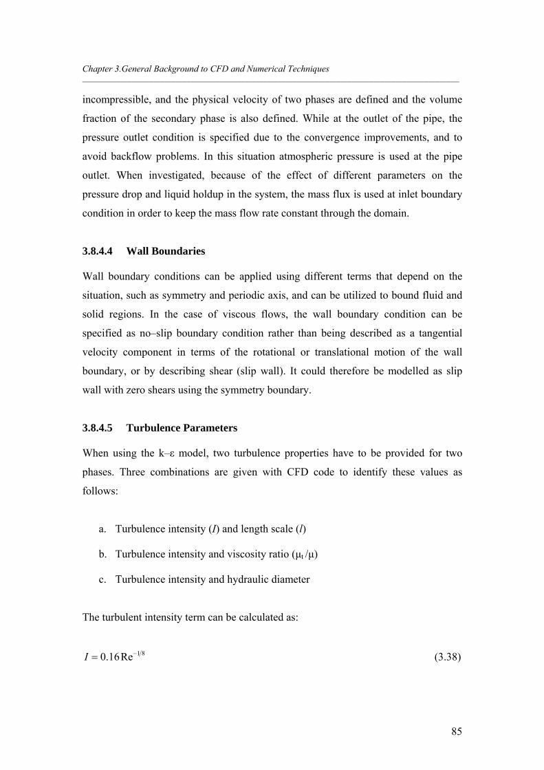
Chapter 3.General Background to CFD and Numerical Techniques _______________________________________________________________________________________________________
85
incompressible, and the physical velocity of two phases are defined and the volume
fraction of the secondary phase is also defined. While at the outlet of the pipe, the
pressure outlet condition is specified due to the convergence improvements, and to
avoid backflow problems. In this situation atmospheric pressure is used at the pipe
outlet. When investigated, because of the effect of different parameters on the
pressure drop and liquid holdup in the system, the mass flux is used at inlet boundary
condition in order to keep the mass flow rate constant through the domain.
3.8.4.4 Wall Boundaries
Wall boundary conditions can be applied using different terms that depend on the
situation, such as symmetry and periodic axis, and can be utilized to bound fluid and
solid regions. In the case of viscous flows, the wall boundary condition can be
specified as no–slip boundary condition rather than being described as a tangential
velocity component in terms of the rotational or translational motion of the wall
boundary, or by describing shear (slip wall). It could therefore be modelled as slip
wall with zero shears using the symmetry boundary.
3.8.4.5 Turbulence Parameters
When using the k–ε model, two turbulence properties have to be provided for two
phases. Three combinations are given with CFD code to identify these values as
follows:
a. Turbulence intensity (I) and length scale (l)
b. Turbulence intensity and viscosity ratio (μt /μ)
c. Turbulence intensity and hydraulic diameter
The turbulent intensity term can be calculated as:
81Re16.0 I (3.38)
Chapter 3.General Background to CFD and Numerical Techniques _______________________________________________________________________________________________________
86
Usually the turbulence intensity is between 1–10%, but sometimes it is greater 10%,
which is considered extremely high. In contrast 1% or less of turbulence intensity is
considered low. The above equation is the best practice for predicting the turbulent
intensity value. In contrast, in the situation of fully developed pipe flows, turbulent
length scales is limited by the flow path length because the turbulent eddies cannot be
greater than the conduit length. Nevertheless, the turbulence length scale can be taken
as between 5–10% of the pipe diameter or can be estimated approximately by the
following equation:
l = 0.07 D (3.39)
where D expresses the pipe diameter and 0.07 is an empirical constant based on the
maximum value of the mixing length in a fully developed turbulent flow (FLUENT
6.2 User’s Guide, 2005).
The turbulent kinetic energy and dissipation rate can be calculated as follows:
2inletIUk (3.40)
l
kC
2323
(3.41)
The turbulent intensity (I) and turbulent length scale (l) can be found from Equations
(3.38) and (3.39), respectively, Uinlet is the mixture velocity at the inlet and Cμ is an
empirical constant given by 0.09.
3.9 Numerical Solver
The commercial CFD codes are mainly based on two categories of solvers, which are
a coupled and segregated solver. In the coupled solver, the governing equations for
momentum, mass, and energy are solved simultaneously, but the segregated solver
equations of transport governing are solved sequentially. Moreover, governing
equations of additional scalars are calculated sequentially for both formulations.
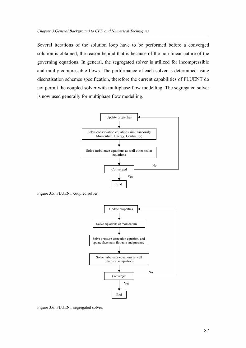
Chapter 3.General Background to CFD and Numerical Techniques _______________________________________________________________________________________________________
87
Several iterations of the solution loop have to be performed before a converged
solution is obtained, the reason behind that is because of the non-linear nature of the
governing equations. In general, the segregated solver is utilized for incompressible
and mildly compressible flows. The performance of each solver is determined using
discretisation schemes specification, therefore the current capabilities of FLUENT do
not permit the coupled solver with multiphase flow modelling. The segregated solver
is now used generally for multiphase flow modelling.
Figure 3.5: FLUENT coupled solver.
Figure 3.6: FLUENT segregated solver.
Yes
No
Update properties
Solve conservation equations simultaneously Momentum, Energy, Continuity)
Solve turbulence equations as well other scalar equations
Converged
End
Yes
No
Update properties
Solve equations of momentum
Solve pressure correction equation, and update face mass flowrate and pressure
Solve turbulence equations as well other scalar equations
Converged
End
Chapter 3.General Background to CFD and Numerical Techniques _______________________________________________________________________________________________________
88
As shown in Figures (3.5 and 3.6), flow diagrams of numerical solvers of both
coupled and segregated solvers, including the steps of each. Usually the solver
performance is obtained by the discretisation schemes specification and it is not likely
to make a priori selection of the solver. Nonetheless, the capabilities of current
FLUENT do not have support for the coupled solver with the multiphase modelling.
The segregated solver, therefore, is often utilized for multiphase modelling and has
been used in this thesis of two–phase flow in pipe simulation.
3.9.1 Discretisation
As referred in section (3.7), most of the CFD codes utilize a finite volume method,
which is able to convert the governing equations to algebraic equations that are solved
numerically. The finite volume approach includes the combination of governing
equations relating to each control volume, which leads to discrete equations that
preserve each quantity based on the control volume. Discretisation of these governing
equations can be demonstrated more simply using the generic transport equation of a
scalar quantity as written in the following form (Ferziger et al., 1999):
SUt
)()()( (3.42)
where (Λ) presents the scalar diffusivity of scalar (), while S describes the source
term.
When integrated with the equation of generic transport over a control volume, the
developing equation usually includes the face values of variables (e, w, n, and s).
These variables are represented in terms of the nodal values of the variable , such as
E ,W ,P ,S , and N. The available CFD codes as FLUENT gives different options
of algorithms that can be used to complete this target in conjunction with first and
second order upwind, power law, third order MUSCL (Monotone Upstream-centered
Scheme for conservation laws), and QUICK (Quadratic Upstream Interpolation for
Convective Kinetics) schemes. More information about these schemes is provided in
FLUENT 6.2 Manual.
Chapter 3.General Background to CFD and Numerical Techniques _______________________________________________________________________________________________________
89
Several discretisation schemes such as the first and second order upwind, as well as
QUICK are used for momentum, turbulence and phase volume fraction. Usually the
first order upwind scheme gives a stable solution, thus results in better convergence
which has less time compared with higher order discretisation schemes.
3.9.2 Under Relaxation
The ultimate equations of discretisation in a finite volume have a linear form, which is
written as follows:
i
iixyx (3.43)
where x and y are linearised constants. This equation is solved iteratively for until
the convergence is obtained. To prevent the calculation from fluctuations, however, it
is necessary to control the difference in consecutive values of . Typically, this can be
achieved using an under relation factor, which minimizes the change of attained
throughout the consecutive iterations. When the Equation (3.43) is modified, then it
can be written as:
oldnew (3.44)
old
newiiixy
(3.45)
where α refers to an under relation factor, which has a value ranged from 0.1 to 1.
3.9.3 Pressure Velocity Coupling
Typically pressure velocity coupling in the CFD solver is solved to develop an
equation for pressure from the continuity discrete equation. There are different
approaches which are based on the pressure velocity algorithm, such as SIMPLE,
SIMPLEC, and PISO. In general, The SIMPLE (semi–implicit pressure linked
equation) algorithm is broadly utilized in existing CFD codes. It employs the
Chapter 3.General Background to CFD and Numerical Techniques _______________________________________________________________________________________________________
90
relationship between velocity and pressure corrections to impose the mass
conservation in consequence to get the pressure. While the velocities are typically
calculated by a segregated solver, it is also coupled with the phases. The equation of
pressure correction is derived based on total volume continuity and is solved.
Following this the pressure and velocities are adjusted to assure the satisfaction of the
continuity constraint (FLUENT 6.2 User’s Guide, 2005).
Therefore, using the SIMPLE algorithm, the equation of pressure velocity is affected
by divergence difficulties, except if some under–relaxation is used. The velocity
components usually are under–relaxed to make this algorithm more powerful. One of
the factors that restrict the use of the SIMPLE algorithm is that the new velocities and
their related fluxes cannot satisfy the momentum balance after the pressure correction
equation is solved. Therefore, the calculation has to be iterated until the balance
equation is fulfilled. The modified form of SIMPLE algorithm has been utilized in
Eulerian–Eulerian simulations in this research as given in more detail in Chapter 5.
Another scheme which is one of the SIMPLE algorithm categories is the PISO
(Pressure–Implicit with Splitting of Operators) scheme. It is derived from the higher
degree of the approximate relation among the velocity and pressure corrections. In
contrast with the SIMPLE algorithm, it has the ability to do two further corrections,
these are skewness and neighbour correction. The advantage of using this algorithm is
that it allows a fast convergence rate and sufficient accuracy without loss (FLUENT
6.2 User’s Guide, 2005).
3.10 Conclusions
In this chapter Computational Fluid Dynamics (CFD) techniques have been reviewed
and their capabilities of modelling two–phase flow also have been summarised. In
addition, an overview of the available CFD codes, turbulence models, and related
issues of modelling two–phase flow were introduced. A detailed description of the
dispersed Multi-fluid flow modelling (Eulerian–Eulerian, Volume of Fluid, and
Eulerian–Lagrangian) was given, including the conservation equations that have been
used in each approach. No studies have been reviewed relating to two–phase flow in
Chapter 3.General Background to CFD and Numerical Techniques _______________________________________________________________________________________________________
91
pipes using CFD simulation. This part will be covered in subsequent chapters, which
will include discussion of droplet hydrodynamics, flow pattern, liquid holdup and
pressure drop.
3.11 Bibliography
Bakker, A. and L. M. Oshinowo (2004). Modeling of turbulence in stirred vessels
using Large Eddy Simulation. Chemical Engineering Research and Design, 82,
1169-1178.
Bakker, A., A. H. Haidari and L. M. Oshinowo (2001). Realize greater benefits from
CFD, fluid/solids handling. AIChE’s CEP magazine, March, 45-53.
Chen, P., M. P. Dudukovic and J. Sanyal (2005). Three-dimensional simulation of
bubble column flows with bubble coalescence and breakup. AIChE Journal, 51,
696-712.
Constantinescu, G. S. and K. D. Squires (2003). LES and DNS investigations of
turbulent flow over a sphere at Re = 10,000. Flow, Turbulence and Combustion,
70, 267-298.
De Schepper, S. C. K., G.J. Heynderickx and G. B. Marin (2008). CFD modeling of
all gas liquid and vapor liquid flow regimes predicted by the Baker chart.
Chemical Engineering Journal, 138(13), 349-357.
Delnoij, E., J. A. M. Kuipers and W. P. M. van Swaaij (1999). A three-dimensional
CFD model for gas-liquid bubble columns. Chemical Engineering Science, 54,
2217-2226.
Domgin, J., D. G. F. Huilier, H. Burnage and P. Gardin (1997). Coupling of a
lagrangian model with a CFD code: Application to the numerical modelling of
the turbulent dispersion of droplets in a turbulent pipe flow. Journal of
Hydraulic Research, 35, 473-488.
Drew, D. A. (1983). Mathematical modeling of two-phase flow. Annual Reviews in
Fluid Mechanics, 15, 261-291.
Ferziger, J. H. and M. Perić (1999). Computational models for fluid dynamics
(Second edition). Springer, Berlin.
FLUENT 6.2 User’s Guide (2005), FLUENT Inc., Lebanon, NH.
Chapter 3.General Background to CFD and Numerical Techniques _______________________________________________________________________________________________________
92
Gaylard, A. (2001). In: Computational fluid dynamics in practice. Rhodes, N.
(Editor). Professional Engineering Publishing.
Hjertager, L. K., B. H. Hjertager and T. Solberg (2002). CFD modelling of fast
chemical reactions in turbulent liquid flows. Computers & Chemical
Engineering, 26(4-5), 507-515.
Hossain, A., J. Naser, A. M. K. McManus and G. Ryan (2003). CFD Investigation of
particle deposition and distribution in a horizontal pipe. Presented at the 3th
international conference on CFD in the Minerals and Process Industries,
Melbourne, Australia, 10-12 December.
Jaworski, Z. and P. Pianko-oprych (2002). Two-phase laminar flow simulations in a
kenics static mixer. The Standard Eulerian and Lagrangian Approaches,
Transactions IChemE, Chemical Engineering Research and Design, Part A, 80,
910-916.
Launder, B. E. and D. B. Spalding (1974). The numerical computation of turbulent
flows, Computer Methods in Applied Mechanics and Engineering, 3(2), 269-
289.
Li, J. (1995). Calcul d’interface affine par morceaux (Piecewise Linear Interface
Calculation). C. R. Acad. Sci. Paris S´er. II, 320, 391–396.
Lopez de Bertodano, M., S. -J. Lee, Jr. R. T. Lahey and D. A. Drew (1990). The
prediction of two-phase distribution phenomena using a Reynolds stress model.
Journal of Fluids Engineering, 112, 107-113.
Morsi, S. A. and A. J. Alexander (1972). An investigation of particle trajectories in
two-phase flow systems. Journal of Fluid Mechanics, 55(2), 193-208.
Noh, W. and P. Woodward (1976). SLIC (simple line interface calculation), in: A.
van de Vooren, P. Zandbergen (Editions.), Proceedings of the 5th International
Conference on Fluid Dynamics, 59: Lecture Notes in Physics, Springer, Berlin,
330–340.
Oberkampf, W. L. and T. G. Trucano (2002). Verification and validation in
computational fluid dynamics. Progress in Aerospace Sciences, 38, 209–272.
Prasad R. O., A. Bakker and E. M. Marshall (1998). Numerical modeling of mixing
processes what can LES offer? Presented at the Annual Meeting of the AIChE,
Session 238, Nov. 15-20, Miami Beach.
Chapter 3.General Background to CFD and Numerical Techniques _______________________________________________________________________________________________________
93
Puckett, E. G. (1991). A volume-of-fluid interface tracking algorithm with
applications to computing shock wave refraction, in: H. Dwyer (Edition),
Proceedings of the 4th International Symposium on Computational Fluid
Dynamics, Davis, CA, 933–938.
Puckett, E. G., A. S. Almgren, J. B. Bell, D. L. Marcus and W. G. Rider (1997). A
high order projection method for tracking fluid interfaces in variable density
incompressible flows. Journal of Computational Physics, 130, 269–282.
Ranade, V. (2002). Computational flow modeling for chemical reactor engineering.
Academic press.
Rashmi G. W., T. S. Y. Choong, S. A. Hussain, M. Khalid and T. G. Chuah (2009).
Numerical study of dispersed oil–water turbulent flow in horizontal tube.
Journal of Petroleum Science and Engineering, 65, 123–128.
Shaw, C. T. (1992). Using computational fluid dynamics. Prentice Hall International
(UK) Ltd.
Ubbink O. (1997). Numerical prediction of two fluid systems with sharp interfaces.
Ph.D. Thesis, Dept. of Mechanical Engineering, Imperial College of Science,
Technology & Medicine.
Van Wachem, B. G. M. and A. E. Almstedt (2003). Methods for multiphase
computational fluid dynamic. Chemical Engineering Journal, 96(1-3), 81-98.
Versteeg, H. K. and W. Malalasekera (1996). Introduction to computational fluid
dynamics: the finite volume method: Addison-Wesley.
Zaleski, S. (2005). Interface tracking-VOF, in: Lecture Given at Course: Industrial
two-phase flow CFD, von Karman Institute for Fluid Dynamics, Belgium.
“Every reasonable effort has been made to acknowledge the owners of copyright
material. I would be pleased to hear from any copyright owner who has been omitted
or incorrectly acknowledged.”
Chapter 4 Numerical Simulation of Flow Pattern and
Droplets Hydrodynamic using Volume of fluid
(VOF) Model
As oil and gas developments are moving into deeper waters, production strategies are
becoming more challenging due to the aggressive environment, and the problems
associated with deep water. In general, oil and gas wells have flowlines that transport
hydrocarbons, water, or chemicals between the platforms and manifolds, satellite
wells and onshore facilities. These flow lines are normally buried on the sea bed.
There is a high risk of water accumulation in the low spot sections during shutdown
operations. During the restart operation, gas contracts and displaces the water,
creating droplets as a result of disturbing the liquid film. This phenomenon of
breaking up of the liquid film in the high velocity gas phase is very complicated.
Understanding the hydrodynamics of droplets in a gas is of engineering importance.
In this chapter, we have attempted to simulate the droplet dynamics for two–phase
flows in a horizontal flow conduit using the Volume of Fluid approach. The objective
of this investigation is to study the flow pattern and drop hydrodynamics in gas
dominated restarts in a low spot flowline. This will assist us to gain a better understanding
of the liquid displacement during restart and to predict the operating conditions which
have a high risk of hydrate formation. Various simulations of air–oil and air–water are
performed to study the effect of different operating parameters. The effect of gas
superficial velocity, liquid patching, low spot depth, and liquid viscosity on flow pattern
and droplet formation is investigated into 0.5 m diameter and 55 m long. Both 2D and 3D
simulations are performed in which all the predicted flow patterns are compared with
Backer flow map.
Chapter 4. Numerical Simulation of Flow Pattern and Droplets Hydrodynamic using VOF model ___________________________________________________________________________________
95
4.1 Introduction
Exploration and production of oil and gas has moved into deep offshore waters with
extreme conditions such as high pressure and low temperature since onshore
reservoirs have been depleted. Typically the pipelines are used to transport the crude
oil and gas from offshore to the processing facilities. In such systems, two–phase flow
is more likely to take place during the transportation of hydrocarbons and gas
condensate. Different flow patterns are expected to be generated, such as stratified,
dispersed, slug, annular flow etc.
As mentioned in Chapter 2, several authors have reported their studies on two–phase
flow in the conduit with different orientation angles (horizontal, vertical, and
inclined). Therefore, the pipeline configuration is typically curved due to the
topography of the sea floor. The accumulated water is most likely to accumulate in
parts of the low sections, which can lead to a high risk of hydrate formation during
restart operations. The consequence of this can result in a blockage to the pipeline,
which is considered a very important challenge to the offshore deep–water
development. The earlier practice of hydrate control strategy is usually based only on
hydrate equilibrium data provided, without considering the other system features,
such as the physical design of the production system, fluid properties, and two–phase
distribution. The consequence of this could lead to quite a conservative approach
providing a significant negative impact on the project economy. Overcautiousness
however is due to the lack of knowledge and understanding of the hydrate formation
and plugging tendencies of carrying two or multi–phase at any flowing conditions.
One of the objectives of flow assurance is to optimize the hydrate control strategy in
order to minimize the capital and operational costs.
The current state–of–the art in the subject of hydrate control has not yet developed to
establish criteria and an experimental methodology that would assist us to find
conclusively whether safe operation within the hydrate zone (expressed by pressure–
temperature plot) is possible or not. Few cases are reported where certain production
systems have been sufficiently operated inside the hydrate area. Moreover, the cause
of such behaviour is due to the natural surfactants, which exist with the crude oil.
Chapter 4. Numerical Simulation of Flow Pattern and Droplets Hydrodynamic using VOF model ___________________________________________________________________________________
96
These surfactants provide self prevention of the hydrate plugging as seen in the
literature review in Chapter 2. Some case studies based on field data have shown that
multi–fluid transportation with up to 30% of water into the hydrate region is possible
without adding any inhibitor. This behaviour is called “self–inhibition through natural
surfactants” in which hydrate formation is not avoided, but under specific conditions
pipeline blockage is prevented by transporting the hydrate as slurry flow.
The first attempt to examine the two–phase flow in a curved pipeline was conducted
by Fitreman (1975). He studied the stability of two–phase gas–liquid flow in the
curved section of a pipe by conducting a theoretical and experimental study.
Leporcher et al. (2002) investigated the hydrate plugging of multi–phase flow in flow
loops consisting of a two parts horizontal section with 140 m, 0.05 m diameter with a
low pipe section about 22 m long and around 1 m depth. The author studied various
parameters, such as levels of stagnant liquid before restart, different gas restart
velocities, pipe geometry, and different fluid systems (gas–water, and gas–water–oil),
to examine the impact on hydrate plugging.
It was found that the most significant case is at the low restart gas velocity throughout
the accumulated stagnant water, where the plugging took place immediately and was
controlled by the gas flow rate. In the case of three phases, it was found that the oil
layer can delay the plugging time or even prevent it, especially in the case of low
water level, while at high gas velocity no hydrate plugging was noted. The author
concluded that the high energy hydrodynamic restart procedure would allow restarting
the production inside the hydrate zone, whereas the low energy restart would assist
hydrate plug formation.
The result obtained provides some preliminary input to the actual field operations.
Therefore, more research is needed in order to investigate the risk of hydrate plugging
in different pipe geometries. Volk et al. (2007) investigated the hydrate plugging of
multi–phase flow in a horizontal stainless steel flow loop of 0.076 m, including the
low section with and without an inhibitor. Different experiments at the low spot were
performed at various operating conditions of restart gas flowrates and water fractions
Chapter 4. Numerical Simulation of Flow Pattern and Droplets Hydrodynamic using VOF model ___________________________________________________________________________________
97
that ranged from 0.15–0.25 ft/s and from 5–75%, respectively. Two different flow
patterns were observed, theses were dispersed and segregated flow. Moreover, low
gas restart velocities had a significant impact on the plugging tendency.
Such systems of multi–phase flow requires a better understanding of multi–phase
transient flow patterns to assist in understanding the mechanisms of hydrate plug
formation. In addition they also examined the effect of water fraction, and found that
the importance of transient flow pattern which depends on the water fraction, liquid
loading, pipe geometry, restart velocity, and two–phase distribution. The author noted
that the water level plays a crucial role in the hydrate plugging in which the
probability of hydrate formation is proportional to the water level. Furthermore, the
plug can take place at a low water fraction, depending on the operating conditions and
the pipe geometry.
Volk et al. (2007) studied also the effect of water salinity, since the produced water
will not be clean, but will be brine with various salinities. The influence of the salt
hydrodynamic is relatively well understood and known however the effects of salinity
on hydrate kinetics, particle agglomeration, and plug formation is not understood.
Different experiments were performed to study the effect of salinity on the plug
development throughout the restart in the low point pipe sections. The experiment
concluded that the salinity had an effect on the hydrate formation rate and also
affected the flow patterns. However, these experiments demonstrated that an
understanding of the transient flow patterns is required when studying hydrate
plugging in low section pipelines. Therefore, further work is needed to provide a
better understanding of the flow pattern risks at low liquid loading.
In this chapter, the Volume of Fluid model is employed to investigate the effects of
restart gas superficial velocity at different liquid patching on the flow pattern, in a 0.5
m diameter and 55 m long tube. All the fluids used are assumed to be incompressible
and isothermal. The Baker flow map is used to find out the accuracy of the obtained
flow pattern. The effects of restart gas velocity, liquid patching and the level of low
sections are studied both with air–water and air–oil two phases flow. A brief
Chapter 4. Numerical Simulation of Flow Pattern and Droplets Hydrodynamic using VOF model ___________________________________________________________________________________
98
comparison between the simulation flow pattern and Baker chart is reported, also
between 2D and 3D simulations.
4.2 Multiphase Flow Modeling
As mentioned before, multiphase flow processes consist of several different flow
patterns according to the operating conditions. Three steps need to be considered
when modelling multiphase flow. The first step is to determine the number of phases.
The next step involves the formulation of the governing equations which describe the
multiphase flow. The numerical simulation of any flow problem requires solving the
basic flow equations that describe the conservation of momentum, mass and energy in
the control volume. The last step in the multiphase flow modelling consists of the
solution of these governing equations.
In order to study the hydrodynamics of droplets and flow patterns in horizontal
pipelines, including low spots, an existing CFD code is used. For this purpose, the
Volume of Fluid (VOF) model in an Eulerian–Eulerian method is chosen for the two–
phase flow simulation, in which the grid is fixed and the fluids are assumed to behave
as continuous media. In the VOF model, an Eulerian scheme is shared by both phases,
combined with a reformulation of the interface forces on a volumetric basis, as will be
illustrated next.
4.2.1 Solution Procedure The VOF model in ANSYS FLUENT 12.1 has been used to simulate the flow pattern
and the droplet formation. In this model, as mentioned before in section (3.8.1.1), the
progress of gas–liquid interface is tracked using the distribution of the liquid fraction
(αl) in the computational cell. It is equal to zero in the gas phase and unity in the
liquid phase. However, the interface of two–phase presents in the cell, where the
liquid fraction ranges from 0−1. The finite volume discretisation scheme is employed
for interface tracking. There are different discretisation schemes available with the
explicit scheme for VOF that are first order upwind, second order upwind,
Compressive Interface Capturing Scheme for Arbitrary Meshes (CICSAM), modified
Chapter 4. Numerical Simulation of Flow Pattern and Droplets Hydrodynamic using VOF model ___________________________________________________________________________________
99
High Resolution Interface Capturing (HRIC), and Quadratic Upstream Interpolation
for Convective Kinetics (QUICK). The CICSAM method was used to track the
interface accurately. The surface tension was taken into account and given a constant
value (0.073 N/m), and the k–ε turbulence model was applied to model the phase
turbulence.
4.2.1.1 Equation of Continuity (conservation of mass)
0.
iut
(4.1)
4.2.1.2 Conservation of Momentum (Navier–Stokes equation)
One momentum equation is shared by all phases, and is solved all through the entire
domain.
iijijii Fguupuuut
)(.).()( (4.2)
The term on the left hand side represents the convection and the other four terms on
the right side represent the pressure, diffusion, the body force of the gravity and the
external body force, respectively.
4.2.1.3 The Volume Fraction Equation
The interface tracking between two phases of gas–liquid is achieved by solving the
continuity equations of the liquid phase volume fraction, which can be written as:
0.
lil U
t
(4.3)
This equation of volume fraction is not solved for the gas phase volume fraction,
which is calculated based on the following constraint:
Chapter 4. Numerical Simulation of Flow Pattern and Droplets Hydrodynamic using VOF model ___________________________________________________________________________________
100
1 lg (4.4)
where g and l are the volume fraction of gas and liquid phase, respectively.
4.2.2 Turbulence Model
The turbulence model of k–ε that is available in ANSYS FLUENT 12.1 was utilized
to model the turbulence in the continuous phase (gas). A turbulence model is
commonly used for simulating turbulence eddies. This model takes into account the
transport of turbulence velocity and length scale. It utilizes a transport equation for the
length scale, which provides a distribution of the length scale even in the case of
complex flow, such as two–phase flow in a pipeline, with which the present research
is concerned.
4.2.3 Physical Properties
At any given cell, the properties and variables of a two–phase mixture are obtained
either by the volume fraction contributions or presented purely. However, the two–
phase mixture properties used in the transport equations are found by the existence of
the gas–liquid phase in each control volume. The density of the mixture in each cell
can be expressed by:
glllggllmix )1( (4.5)
And the viscosity of the mixture is calculated in the same manner:
glllggllmix )1( (4.6)
where l , l , g and g are the density and viscosity of liquid and gas phase,
respectively.
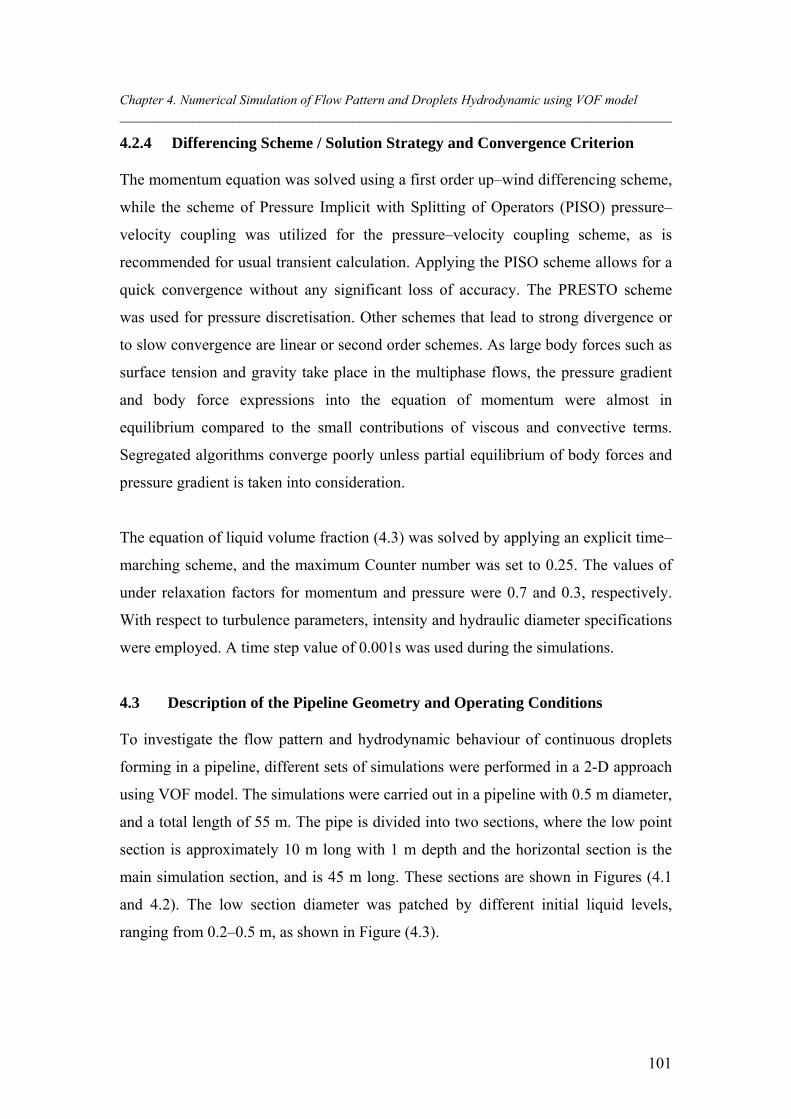
Chapter 4. Numerical Simulation of Flow Pattern and Droplets Hydrodynamic using VOF model ___________________________________________________________________________________
101
4.2.4 Differencing Scheme / Solution Strategy and Convergence Criterion
The momentum equation was solved using a first order up–wind differencing scheme,
while the scheme of Pressure Implicit with Splitting of Operators (PISO) pressure–
velocity coupling was utilized for the pressure–velocity coupling scheme, as is
recommended for usual transient calculation. Applying the PISO scheme allows for a
quick convergence without any significant loss of accuracy. The PRESTO scheme
was used for pressure discretisation. Other schemes that lead to strong divergence or
to slow convergence are linear or second order schemes. As large body forces such as
surface tension and gravity take place in the multiphase flows, the pressure gradient
and body force expressions into the equation of momentum were almost in
equilibrium compared to the small contributions of viscous and convective terms.
Segregated algorithms converge poorly unless partial equilibrium of body forces and
pressure gradient is taken into consideration.
The equation of liquid volume fraction (4.3) was solved by applying an explicit time–
marching scheme, and the maximum Counter number was set to 0.25. The values of
under relaxation factors for momentum and pressure were 0.7 and 0.3, respectively.
With respect to turbulence parameters, intensity and hydraulic diameter specifications
were employed. A time step value of 0.001s was used during the simulations.
4.3 Description of the Pipeline Geometry and Operating Conditions
To investigate the flow pattern and hydrodynamic behaviour of continuous droplets
forming in a pipeline, different sets of simulations were performed in a 2-D approach
using VOF model. The simulations were carried out in a pipeline with 0.5 m diameter,
and a total length of 55 m. The pipe is divided into two sections, where the low point
section is approximately 10 m long with 1 m depth and the horizontal section is the
main simulation section, and is 45 m long. These sections are shown in Figures (4.1
and 4.2). The low section diameter was patched by different initial liquid levels,
ranging from 0.2–0.5 m, as shown in Figure (4.3).
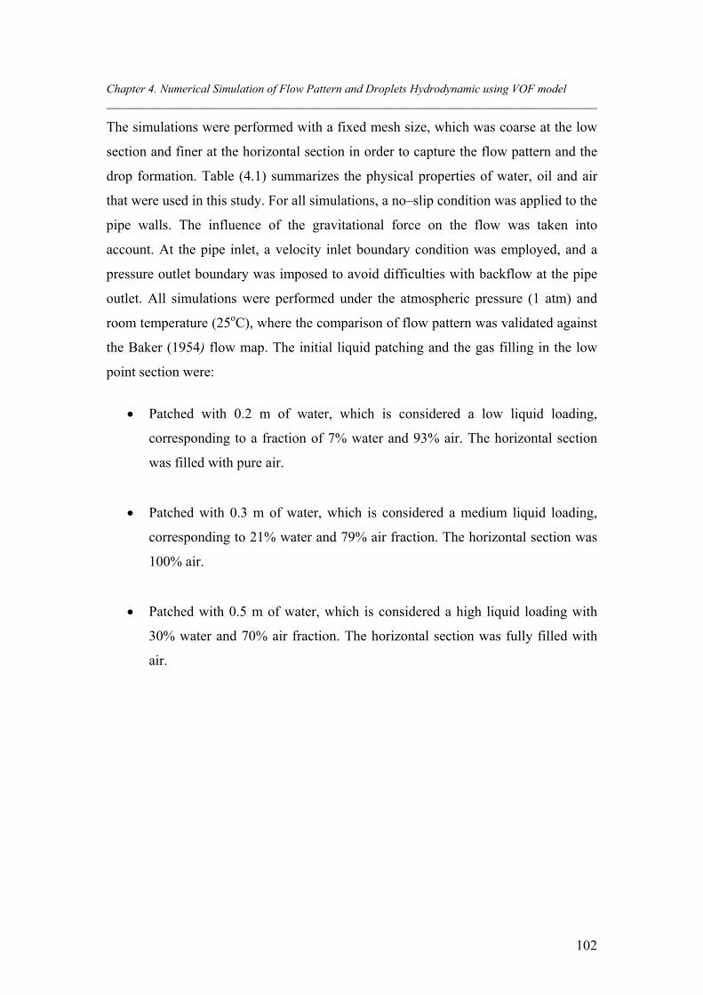
Chapter 4. Numerical Simulation of Flow Pattern and Droplets Hydrodynamic using VOF model ___________________________________________________________________________________
102
The simulations were performed with a fixed mesh size, which was coarse at the low
section and finer at the horizontal section in order to capture the flow pattern and the
drop formation. Table (4.1) summarizes the physical properties of water, oil and air
that were used in this study. For all simulations, a no–slip condition was applied to the
pipe walls. The influence of the gravitational force on the flow was taken into
account. At the pipe inlet, a velocity inlet boundary condition was employed, and a
pressure outlet boundary was imposed to avoid difficulties with backflow at the pipe
outlet. All simulations were performed under the atmospheric pressure (1 atm) and
room temperature (25oC), where the comparison of flow pattern was validated against
the Baker (1954) flow map. The initial liquid patching and the gas filling in the low
point section were:
Patched with 0.2 m of water, which is considered a low liquid loading,
corresponding to a fraction of 7% water and 93% air. The horizontal section
was filled with pure air.
Patched with 0.3 m of water, which is considered a medium liquid loading,
corresponding to 21% water and 79% air fraction. The horizontal section was
100% air.
Patched with 0.5 m of water, which is considered a high liquid loading with
30% water and 70% air fraction. The horizontal section was fully filled with
air.
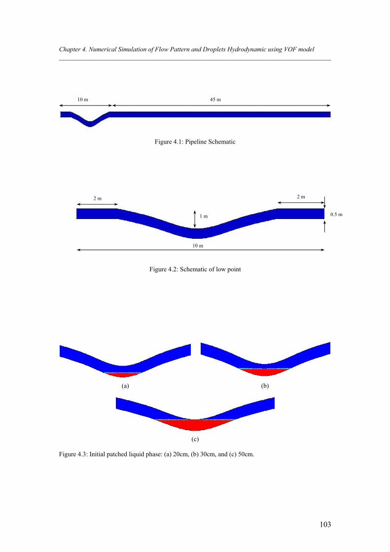
Chapter 4. Numerical Simulation of Flow Pattern and Droplets Hydrodynamic using VOF model ___________________________________________________________________________________
103
Figure 4.1: Pipeline Schematic
Figure 4.2: Schematic of low point
(a) (b)
(c)
Figure 4.3: Initial patched liquid phase: (a) 20cm, (b) 30cm, and (c) 50cm.
2 m 2 m
0.5 m 1 m
10 m
45 m 10 m
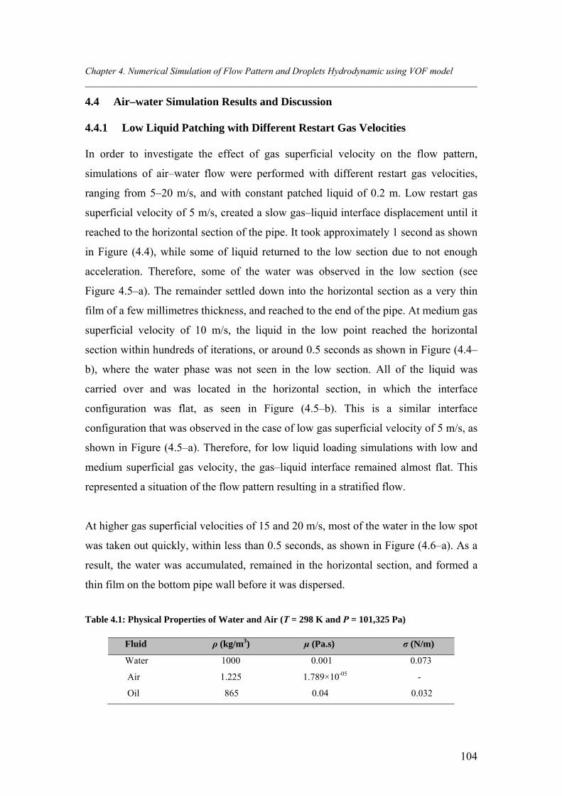
Chapter 4. Numerical Simulation of Flow Pattern and Droplets Hydrodynamic using VOF model ___________________________________________________________________________________
104
4.4 Air–water Simulation Results and Discussion
4.4.1 Low Liquid Patching with Different Restart Gas Velocities
In order to investigate the effect of gas superficial velocity on the flow pattern,
simulations of air–water flow were performed with different restart gas velocities,
ranging from 5–20 m/s, and with constant patched liquid of 0.2 m. Low restart gas
superficial velocity of 5 m/s, created a slow gas–liquid interface displacement until it
reached to the horizontal section of the pipe. It took approximately 1 second as shown
in Figure (4.4), while some of liquid returned to the low section due to not enough
acceleration. Therefore, some of the water was observed in the low section (see
Figure 4.5–a). The remainder settled down into the horizontal section as a very thin
film of a few millimetres thickness, and reached to the end of the pipe. At medium gas
superficial velocity of 10 m/s, the liquid in the low point reached the horizontal
section within hundreds of iterations, or around 0.5 seconds as shown in Figure (4.4–
b), where the water phase was not seen in the low section. All of the liquid was
carried over and was located in the horizontal section, in which the interface
configuration was flat, as seen in Figure (4.5–b). This is a similar interface
configuration that was observed in the case of low gas superficial velocity of 5 m/s, as
shown in Figure (4.5–a). Therefore, for low liquid loading simulations with low and
medium superficial gas velocity, the gas–liquid interface remained almost flat. This
represented a situation of the flow pattern resulting in a stratified flow.
At higher gas superficial velocities of 15 and 20 m/s, most of the water in the low spot
was taken out quickly, within less than 0.5 seconds, as shown in Figure (4.6–a). As a
result, the water was accumulated, remained in the horizontal section, and formed a
thin film on the bottom pipe wall before it was dispersed.
Table 4.1: Physical Properties of Water and Air (T = 298 K and P = 101,325 Pa)
Fluid ρ (kg/m3) μ (Pa.s) σ (N/m)
Water 1000 0.001 0.073
Air 1.225 1.789×10-05 -
Oil 865 0.04 0.032
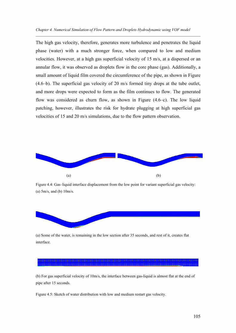
Chapter 4. Numerical Simulation of Flow Pattern and Droplets Hydrodynamic using VOF model ___________________________________________________________________________________
105
The high gas velocity, therefore, generates more turbulence and penetrates the liquid
phase (water) with a much stronger force, when compared to low and medium
velocities. However, at a high gas superficial velocity of 15 m/s, at a dispersed or an
annular flow, it was observed as droplets flow in the core phase (gas). Additionally, a
small amount of liquid film covered the circumference of the pipe, as shown in Figure
(4.6–b). The superficial gas velocity of 20 m/s formed tiny drops at the tube outlet,
and more drops were expected to form as the film continues to flow. The generated
flow was considered as churn flow, as shown in Figure (4.6–c). The low liquid
patching, however, illustrates the risk for hydrate plugging at high superficial gas
velocities of 15 and 20 m/s simulations, due to the flow pattern observation.
(a) (b) Figure 4.4: Gas–liquid interface displacement from the low point for variant superficial gas velocity:
(a) 5m/s, and (b) 10m/s.
(a) Some of the water, is remaining in the low section after 35 seconds, and rest of it, creates flat
interface.
(b) For gas superficial velocity of 10m/s, the interface between gas-liquid is almost flat at the end of
pipe after 15 seconds.
Figure 4.5: Sketch of water distribution with low and medium restart gas velocity.
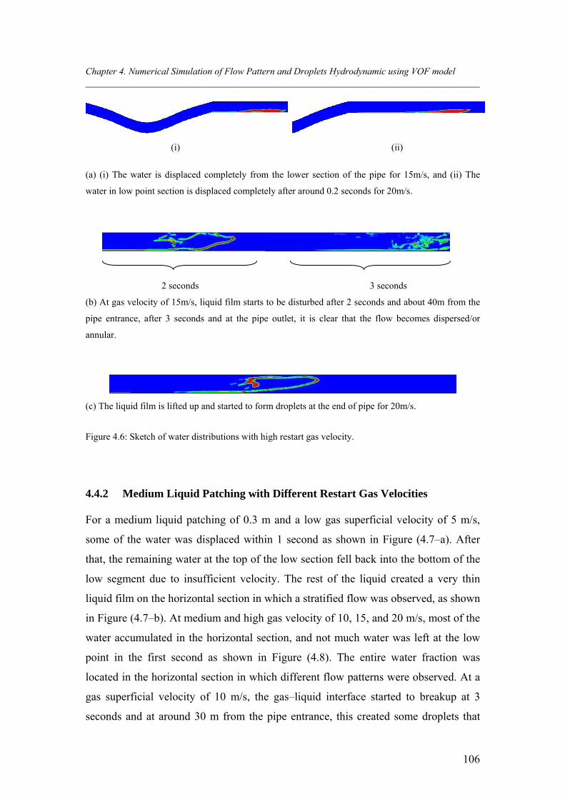
Chapter 4. Numerical Simulation of Flow Pattern and Droplets Hydrodynamic using VOF model ___________________________________________________________________________________
106
(i) (ii)
(a) (i) The water is displaced completely from the lower section of the pipe for 15m/s, and (ii) The
water in low point section is displaced completely after around 0.2 seconds for 20m/s.
2 seconds 3 seconds
(b) At gas velocity of 15m/s, liquid film starts to be disturbed after 2 seconds and about 40m from the
pipe entrance, after 3 seconds and at the pipe outlet, it is clear that the flow becomes dispersed/or
annular.
(c) The liquid film is lifted up and started to form droplets at the end of pipe for 20m/s.
Figure 4.6: Sketch of water distributions with high restart gas velocity.
4.4.2 Medium Liquid Patching with Different Restart Gas Velocities
For a medium liquid patching of 0.3 m and a low gas superficial velocity of 5 m/s,
some of the water was displaced within 1 second as shown in Figure (4.7–a). After
that, the remaining water at the top of the low section fell back into the bottom of the
low segment due to insufficient velocity. The rest of the liquid created a very thin
liquid film on the horizontal section in which a stratified flow was observed, as shown
in Figure (4.7–b). At medium and high gas velocity of 10, 15, and 20 m/s, most of the
water accumulated in the horizontal section, and not much water was left at the low
point in the first second as shown in Figure (4.8). The entire water fraction was
located in the horizontal section in which different flow patterns were observed. At a
gas superficial velocity of 10 m/s, the gas–liquid interface started to breakup at 3
seconds and at around 30 m from the pipe entrance, this created some droplets that
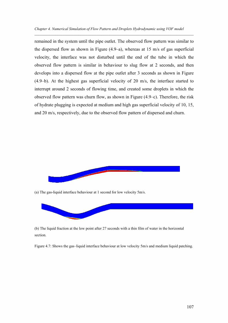
Chapter 4. Numerical Simulation of Flow Pattern and Droplets Hydrodynamic using VOF model ___________________________________________________________________________________
107
remained in the system until the pipe outlet. The observed flow pattern was similar to
the dispersed flow as shown in Figure (4.9–a), whereas at 15 m/s of gas superficial
velocity, the interface was not disturbed until the end of the tube in which the
observed flow pattern is similar in behaviour to slug flow at 2 seconds, and then
develops into a dispersed flow at the pipe outlet after 3 seconds as shown in Figure
(4.9–b). At the highest gas superficial velocity of 20 m/s, the interface started to
interrupt around 2 seconds of flowing time, and created some droplets in which the
observed flow pattern was churn flow, as shown in Figure (4.9–c). Therefore, the risk
of hydrate plugging is expected at medium and high gas superficial velocity of 10, 15,
and 20 m/s, respectively, due to the observed flow pattern of dispersed and churn.
(a) The gas-liquid interface behaviour at 1 second for low velocity 5m/s.
(b) The liquid fraction at the low point after 27 seconds with a thin film of water in the horizontal
section.
Figure 4.7: Shows the gas–liquid interface behaviour at low velocity 5m/s and medium liquid patching.
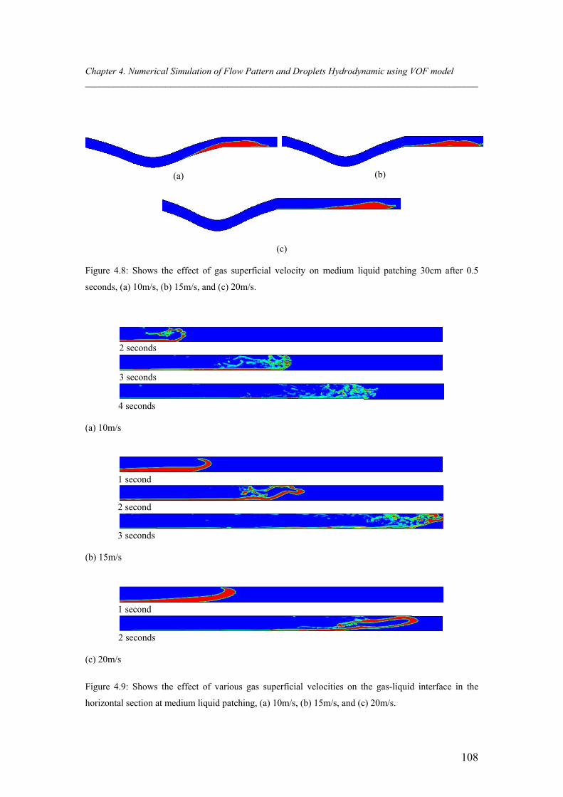
Chapter 4. Numerical Simulation of Flow Pattern and Droplets Hydrodynamic using VOF model ___________________________________________________________________________________
108
(a) (b)
(c)
Figure 4.8: Shows the effect of gas superficial velocity on medium liquid patching 30cm after 0.5
seconds, (a) 10m/s, (b) 15m/s, and (c) 20m/s.
2 seconds
3 seconds
4 seconds (a) 10m/s
1 second
2 second
3 seconds
(b) 15m/s
1 second
2 seconds (c) 20m/s
Figure 4.9: Shows the effect of various gas superficial velocities on the gas-liquid interface in the
horizontal section at medium liquid patching, (a) 10m/s, (b) 15m/s, and (c) 20m/s.
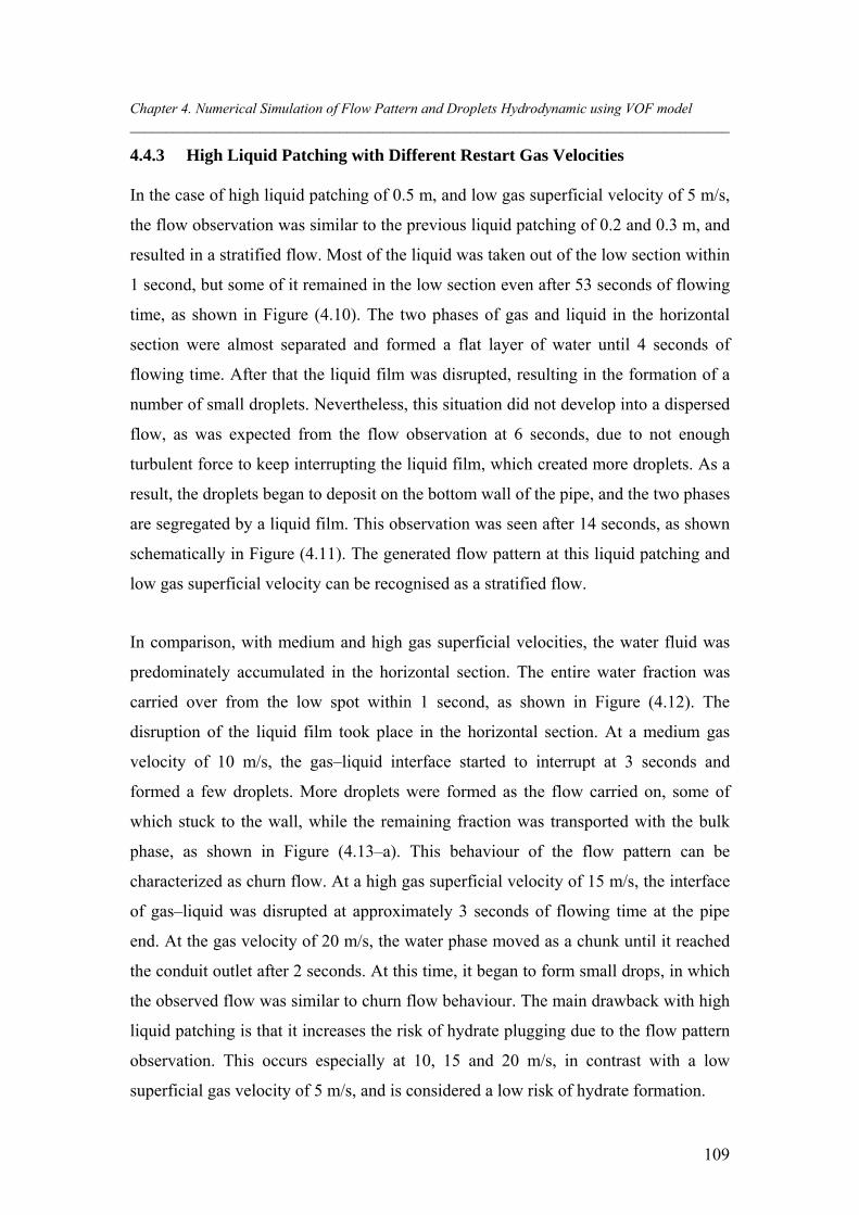
Chapter 4. Numerical Simulation of Flow Pattern and Droplets Hydrodynamic using VOF model ___________________________________________________________________________________
109
4.4.3 High Liquid Patching with Different Restart Gas Velocities
In the case of high liquid patching of 0.5 m, and low gas superficial velocity of 5 m/s,
the flow observation was similar to the previous liquid patching of 0.2 and 0.3 m, and
resulted in a stratified flow. Most of the liquid was taken out of the low section within
1 second, but some of it remained in the low section even after 53 seconds of flowing
time, as shown in Figure (4.10). The two phases of gas and liquid in the horizontal
section were almost separated and formed a flat layer of water until 4 seconds of
flowing time. After that the liquid film was disrupted, resulting in the formation of a
number of small droplets. Nevertheless, this situation did not develop into a dispersed
flow, as was expected from the flow observation at 6 seconds, due to not enough
turbulent force to keep interrupting the liquid film, which created more droplets. As a
result, the droplets began to deposit on the bottom wall of the pipe, and the two phases
are segregated by a liquid film. This observation was seen after 14 seconds, as shown
schematically in Figure (4.11). The generated flow pattern at this liquid patching and
low gas superficial velocity can be recognised as a stratified flow.
In comparison, with medium and high gas superficial velocities, the water fluid was
predominately accumulated in the horizontal section. The entire water fraction was
carried over from the low spot within 1 second, as shown in Figure (4.12). The
disruption of the liquid film took place in the horizontal section. At a medium gas
velocity of 10 m/s, the gas–liquid interface started to interrupt at 3 seconds and
formed a few droplets. More droplets were formed as the flow carried on, some of
which stuck to the wall, while the remaining fraction was transported with the bulk
phase, as shown in Figure (4.13–a). This behaviour of the flow pattern can be
characterized as churn flow. At a high gas superficial velocity of 15 m/s, the interface
of gas–liquid was disrupted at approximately 3 seconds of flowing time at the pipe
end. At the gas velocity of 20 m/s, the water phase moved as a chunk until it reached
the conduit outlet after 2 seconds. At this time, it began to form small drops, in which
the observed flow was similar to churn flow behaviour. The main drawback with high
liquid patching is that it increases the risk of hydrate plugging due to the flow pattern
observation. This occurs especially at 10, 15 and 20 m/s, in contrast with a low
superficial gas velocity of 5 m/s, and is considered a low risk of hydrate formation.
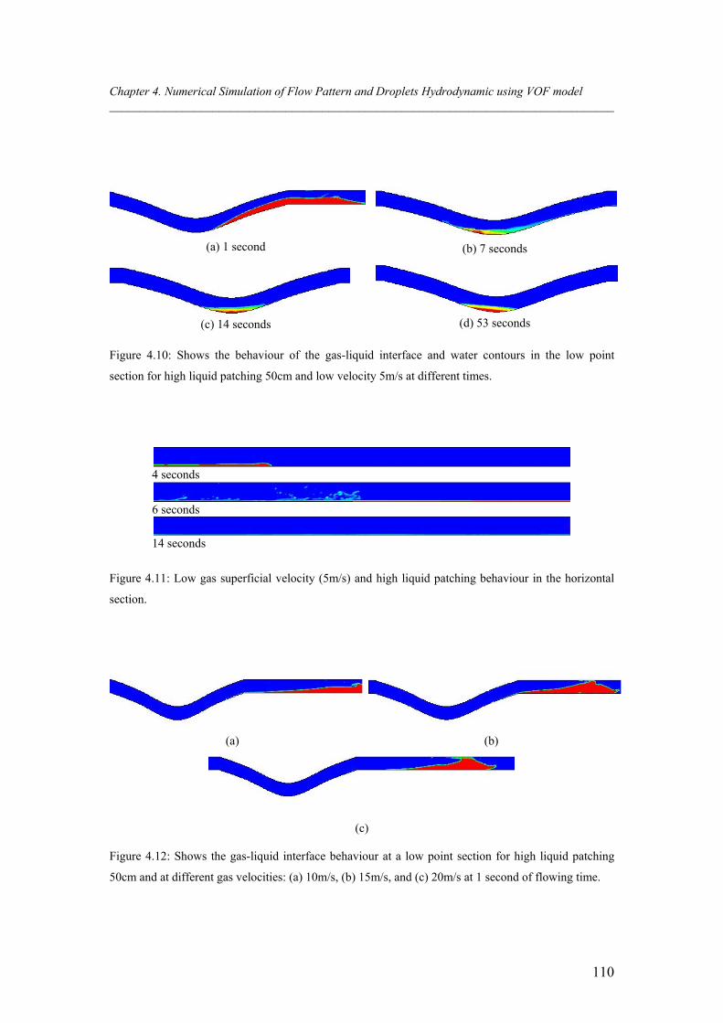
Chapter 4. Numerical Simulation of Flow Pattern and Droplets Hydrodynamic using VOF model ___________________________________________________________________________________
110
(a) 1 second (b) 7 seconds
(c) 14 seconds (d) 53 seconds
Figure 4.10: Shows the behaviour of the gas-liquid interface and water contours in the low point
section for high liquid patching 50cm and low velocity 5m/s at different times.
4 seconds
6 seconds
14 seconds
Figure 4.11: Low gas superficial velocity (5m/s) and high liquid patching behaviour in the horizontal
section.
(a) (b)
(c)
Figure 4.12: Shows the gas-liquid interface behaviour at a low point section for high liquid patching
50cm and at different gas velocities: (a) 10m/s, (b) 15m/s, and (c) 20m/s at 1 second of flowing time.
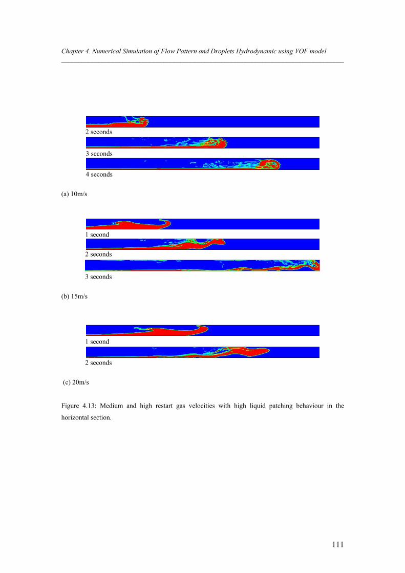
Chapter 4. Numerical Simulation of Flow Pattern and Droplets Hydrodynamic using VOF model ___________________________________________________________________________________
111
2 seconds
3 seconds
4 seconds
(a) 10m/s
1 second
2 seconds
3 seconds
(b) 15m/s
1 second
2 seconds
(c) 20m/s
Figure 4.13: Medium and high restart gas velocities with high liquid patching behaviour in the
horizontal section.
Chapter 4. Numerical Simulation of Flow Pattern and Droplets Hydrodynamic using VOF model ___________________________________________________________________________________
112
4.4.4 Compare the Flow Pattern Simulation with Flow Map for 1m Low
Section Depth
In this work Baker’s flow map in Figure (4.14) is used to identify and compare the
obtained flow pattern as a result of CFD two–phase flow simulation. The flow chart
demonstrates the various boundaries of flow pattern zones as functions of a mass flux
of gas, which is expressed by (G), and the ratio of mass fluxes of liquid and gas phase,
which is expressed via (L/G). The dimensionless parameters ψ and λ are expressed by
Equation (4.7) and (4.8), respectively. They are included when the gas–liquid
combination is different from the standard combination, at which both parameters are
equal to unity, such as in this case where the gas and liquid are defined by air and
water.
31
2
L
W
W
Lw
(4.7)
5.0
W
L
A
G
(4.8)
In all simulation cases, the flow pattern of two–phase air–water flow was obtained
under the atmospheric pressure (101.325 kPa) and room temperature (298 k). The
mass flux of each phase of air and water was calculated to find out the corresponding
flow pattern according to the Baker flow map. Based on the physical properties of
each phase of air and water, the dimensionless parameters (ψ, λ) are equal to 1 in this
situation. In the case of low liquid patching (0.2m), Table (4.2) presents the flow
pattern obtained from different cases of simulation as a result of various restart gas
superficial velocities.
As can be seen from Table (4.2) the predicted flow patterns using the Baker chart are
quite adequate compared with the CFD simulations, especially at low and medium gas
superficial velocities of 5 and 10 m/s respectively. At higher gas velocities all the
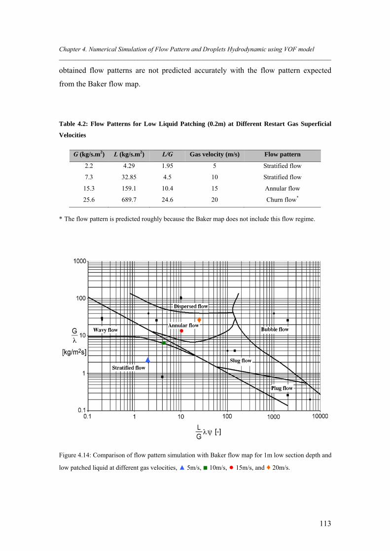
Chapter 4. Numerical Simulation of Flow Pattern and Droplets Hydrodynamic using VOF model ___________________________________________________________________________________
113
obtained flow patterns are not predicted accurately with the flow pattern expected
from the Baker flow map.
Table 4.2: Flow Patterns for Low Liquid Patching (0.2m) at Different Restart Gas Superficial
Velocities
G (kg/s.m2) L (kg/s.m2) L/G Gas velocity (m/s) Flow pattern
2.2 4.29 1.95 5 Stratified flow
7.3 32.85 4.5 10 Stratified flow
15.3 159.1 10.4 15 Annular flow
25.6 689.7 24.6 20 Churn flow*
* The flow pattern is predicted roughly because the Baker map does not include this flow regime.
Figure 4.14: Comparison of flow pattern simulation with Baker flow map for 1m low section depth and
low patched liquid at different gas velocities, ▲ 5m/s, ■ 10m/s, ● 15m/s, and ♦ 20m/s.
▲
■
●♦
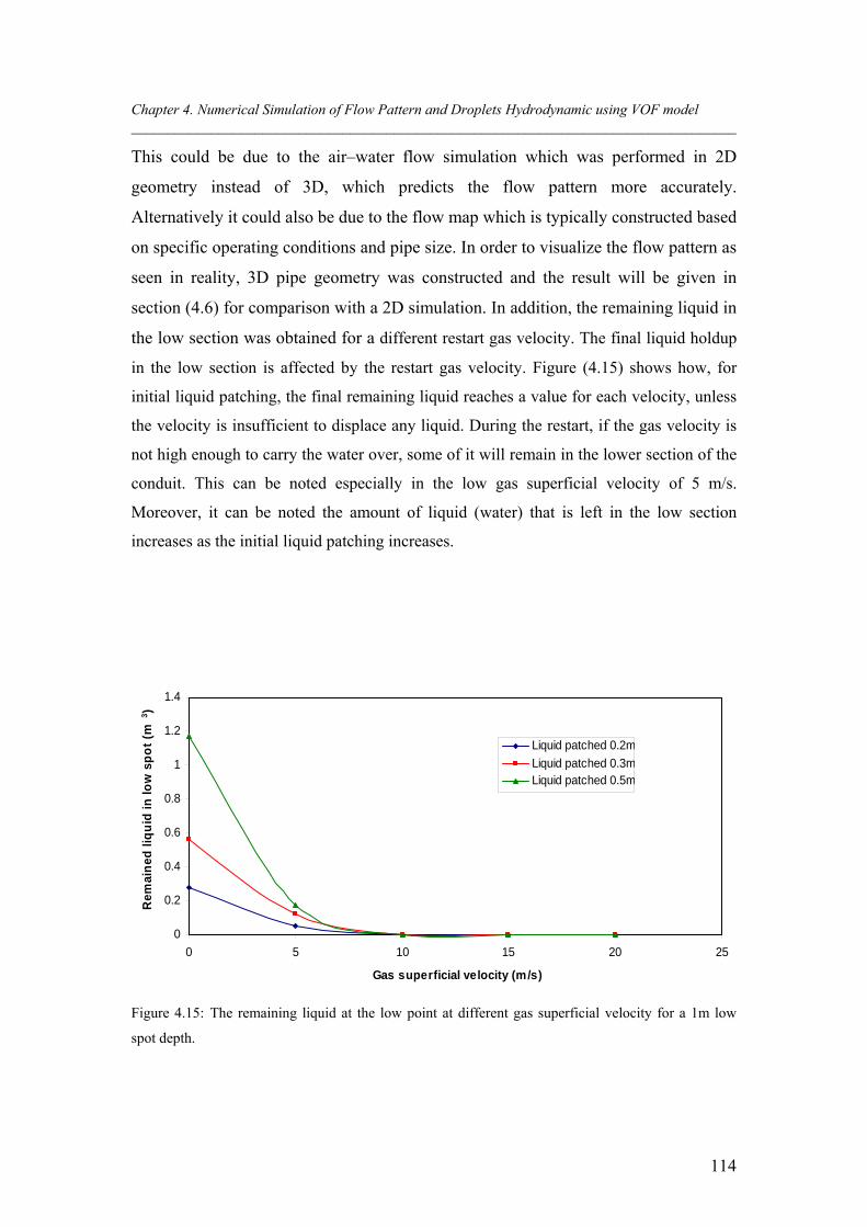
Chapter 4. Numerical Simulation of Flow Pattern and Droplets Hydrodynamic using VOF model ___________________________________________________________________________________
114
This could be due to the air–water flow simulation which was performed in 2D
geometry instead of 3D, which predicts the flow pattern more accurately.
Alternatively it could also be due to the flow map which is typically constructed based
on specific operating conditions and pipe size. In order to visualize the flow pattern as
seen in reality, 3D pipe geometry was constructed and the result will be given in
section (4.6) for comparison with a 2D simulation. In addition, the remaining liquid in
the low section was obtained for a different restart gas velocity. The final liquid holdup
in the low section is affected by the restart gas velocity. Figure (4.15) shows how, for
initial liquid patching, the final remaining liquid reaches a value for each velocity, unless
the velocity is insufficient to displace any liquid. During the restart, if the gas velocity is
not high enough to carry the water over, some of it will remain in the lower section of the
conduit. This can be noted especially in the low gas superficial velocity of 5 m/s.
Moreover, it can be noted the amount of liquid (water) that is left in the low section
increases as the initial liquid patching increases.
0
0.2
0.4
0.6
0.8
1
1.2
1.4
0 5 10 15 20 25
Gas superficial velocity (m/s)
Rem
ain
ed li
qu
id in
low
sp
ot
(m3)
Liquid patched 0.2m
Liquid patched 0.3mLiquid patched 0.5m
Figure 4.15: The remaining liquid at the low point at different gas superficial velocity for a 1m low
spot depth.
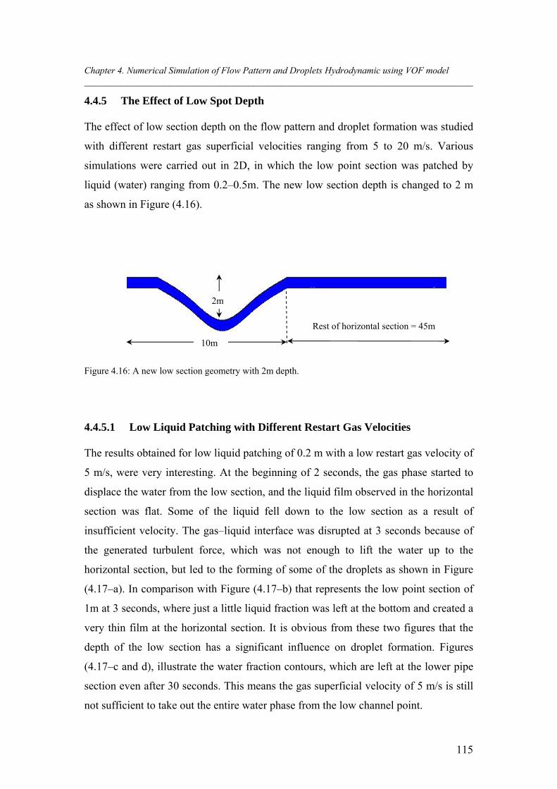
Chapter 4. Numerical Simulation of Flow Pattern and Droplets Hydrodynamic using VOF model ___________________________________________________________________________________
115
4.4.5 The Effect of Low Spot Depth
The effect of low section depth on the flow pattern and droplet formation was studied
with different restart gas superficial velocities ranging from 5 to 20 m/s. Various
simulations were carried out in 2D, in which the low point section was patched by
liquid (water) ranging from 0.2–0.5m. The new low section depth is changed to 2 m
as shown in Figure (4.16).
Figure 4.16: A new low section geometry with 2m depth.
4.4.5.1 Low Liquid Patching with Different Restart Gas Velocities
The results obtained for low liquid patching of 0.2 m with a low restart gas velocity of
5 m/s, were very interesting. At the beginning of 2 seconds, the gas phase started to
displace the water from the low section, and the liquid film observed in the horizontal
section was flat. Some of the liquid fell down to the low section as a result of
insufficient velocity. The gas–liquid interface was disrupted at 3 seconds because of
the generated turbulent force, which was not enough to lift the water up to the
horizontal section, but led to the forming of some of the droplets as shown in Figure
(4.17–a). In comparison with Figure (4.17–b) that represents the low point section of
1m at 3 seconds, where just a little liquid fraction was left at the bottom and created a
very thin film at the horizontal section. It is obvious from these two figures that the
depth of the low section has a significant influence on droplet formation. Figures
(4.17–c and d), illustrate the water fraction contours, which are left at the lower pipe
section even after 30 seconds. This means the gas superficial velocity of 5 m/s is still
not sufficient to take out the entire water phase from the low channel point.
2m
10m
Rest of horizontal section = 45m
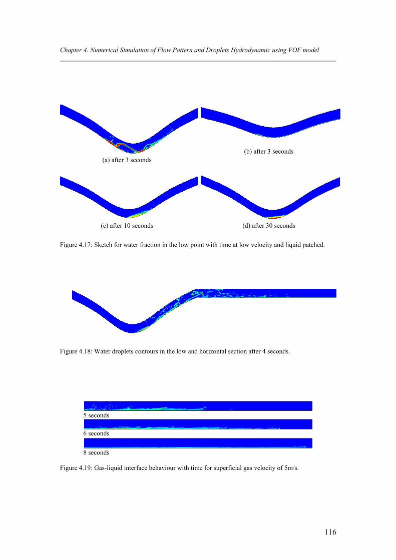
Chapter 4. Numerical Simulation of Flow Pattern and Droplets Hydrodynamic using VOF model ___________________________________________________________________________________
116
(a) after 3 seconds
(b) after 3 seconds
(c) after 10 seconds (d) after 30 seconds
Figure 4.17: Sketch for water fraction in the low point with time at low velocity and liquid patched.
Figure 4.18: Water droplets contours in the low and horizontal section after 4 seconds.
5 seconds
6 seconds
8 seconds Figure 4.19: Gas-liquid interface behaviour with time for superficial gas velocity of 5m/s.
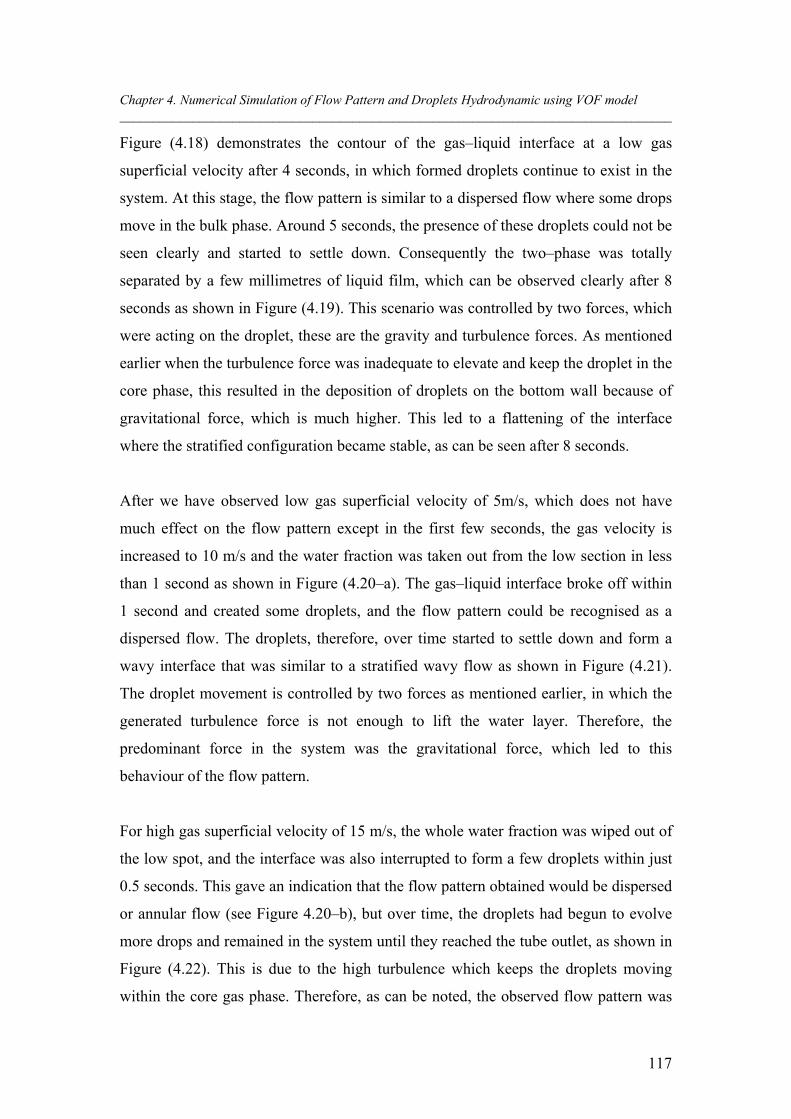
Chapter 4. Numerical Simulation of Flow Pattern and Droplets Hydrodynamic using VOF model ___________________________________________________________________________________
117
Figure (4.18) demonstrates the contour of the gas–liquid interface at a low gas
superficial velocity after 4 seconds, in which formed droplets continue to exist in the
system. At this stage, the flow pattern is similar to a dispersed flow where some drops
move in the bulk phase. Around 5 seconds, the presence of these droplets could not be
seen clearly and started to settle down. Consequently the two–phase was totally
separated by a few millimetres of liquid film, which can be observed clearly after 8
seconds as shown in Figure (4.19). This scenario was controlled by two forces, which
were acting on the droplet, these are the gravity and turbulence forces. As mentioned
earlier when the turbulence force was inadequate to elevate and keep the droplet in the
core phase, this resulted in the deposition of droplets on the bottom wall because of
gravitational force, which is much higher. This led to a flattening of the interface
where the stratified configuration became stable, as can be seen after 8 seconds.
After we have observed low gas superficial velocity of 5m/s, which does not have
much effect on the flow pattern except in the first few seconds, the gas velocity is
increased to 10 m/s and the water fraction was taken out from the low section in less
than 1 second as shown in Figure (4.20–a). The gas–liquid interface broke off within
1 second and created some droplets, and the flow pattern could be recognised as a
dispersed flow. The droplets, therefore, over time started to settle down and form a
wavy interface that was similar to a stratified wavy flow as shown in Figure (4.21).
The droplet movement is controlled by two forces as mentioned earlier, in which the
generated turbulence force is not enough to lift the water layer. Therefore, the
predominant force in the system was the gravitational force, which led to this
behaviour of the flow pattern.
For high gas superficial velocity of 15 m/s, the whole water fraction was wiped out of
the low spot, and the interface was also interrupted to form a few droplets within just
0.5 seconds. This gave an indication that the flow pattern obtained would be dispersed
or annular flow (see Figure 4.20–b), but over time, the droplets had begun to evolve
more drops and remained in the system until they reached the tube outlet, as shown in
Figure (4.22). This is due to the high turbulence which keeps the droplets moving
within the core gas phase. Therefore, as can be noted, the observed flow pattern was
Chapter 4. Numerical Simulation of Flow Pattern and Droplets Hydrodynamic using VOF model ___________________________________________________________________________________
118
dispersed flow. The same observation was noted at a gas superficial velocity of 20
m/s as shown in Figure (4.23).
(a) at 0.5 seconds (b) at 0.5 seconds Figure 4.20: Sketch for water fraction in the low point with time for different gas velocities: (a) 10m/s
and (b) 15m/s.
1 second
2 seconds
3 seconds
4 seconds Figure 4.21: Gas-liquid interface behaviour with time for superficial gas velocity of 10m/s.
1 second
2 seconds
2.8 seconds Figure 4.22: Gas–liquid interface behaviour with time for gas superficial velocity of 15m/s.
1 second
2 seconds
2.5 seconds Figure 4.23: The gas–liquid interface behaviour with time for gas superficial velocity of 20m/s.
Chapter 4. Numerical Simulation of Flow Pattern and Droplets Hydrodynamic using VOF model ___________________________________________________________________________________
119
4.4.5.2 Medium Liquid Patching with Different Restart Gas Velocities
When the liquid patching increased to 0.3 m, almost 1.5 times that of low liquid
patching, the flow behaviour and droplets hydrodynamics were investigated at
different operating conditions of restart gas superficial velocity. Figure (4.24)
demonstrates the liquid behaviour at low gas superficial velocity of 5 m/s, which was
inadequate to take the whole water fraction out of the low point. It was expected that
the low gas velocity of 5 m/s is insufficient to take the water out since it had the same
behaviour at low liquid patching.
Figure (4.24) shows the formation of small droplets at the low point after around 3
seconds. These droplets began to progress in the first 5 m of the horizontal section as
shown in Figure (4.25), in which the obtained two–phase behaviour at 4 seconds was
comparable to the previous simulation of low liquid patching, as seen in Figure (4.18).
Subsequently the droplets started to fall back because of insufficient acceleration to
carry on the water phase. They deposited and created a wavy flow at around 6 seconds
as shown in Figure (4.25). The liquid fraction in the low section started to settle down
after 10 seconds as shown in Figure (4.24–k and l), as well as in the horizontal section
where the water phase most likely spread over the total length of 45 m. This water
layer was only a few millimetres and became completely flattened after 8 seconds.
The observed flow pattern can be described as a stratified flow as shown in Figure
(4.25).
It can be concluded that the behaviour of two–phase flow at medium liquid patching
is quite similar to low liquid patching in terms of droplet formation and deposition
time, as well as the flow behaviour which is exhibited by small droplets and waves on
the gas–liquid interface.
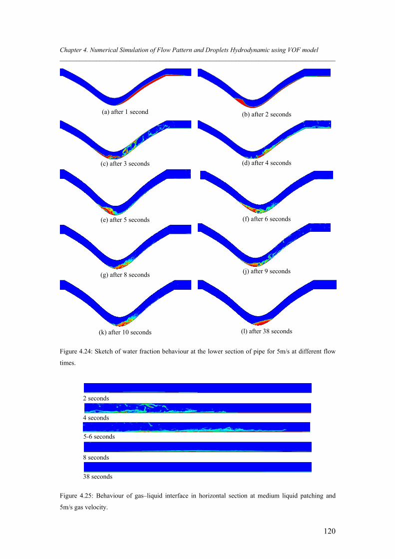
Chapter 4. Numerical Simulation of Flow Pattern and Droplets Hydrodynamic using VOF model ___________________________________________________________________________________
120
(a) after 1 second (b) after 2 seconds
(c) after 3 seconds
(d) after 4 seconds
(e) after 5 seconds
(f) after 6 seconds
(g) after 8 seconds
(j) after 9 seconds
(k) after 10 seconds (l) after 38 seconds
Figure 4.24: Sketch of water fraction behaviour at the lower section of pipe for 5m/s at different flow
times.
2 seconds
4 seconds
5-6 seconds
8 seconds
38 seconds
Figure 4.25: Behaviour of gas–liquid interface in horizontal section at medium liquid patching and
5m/s gas velocity.
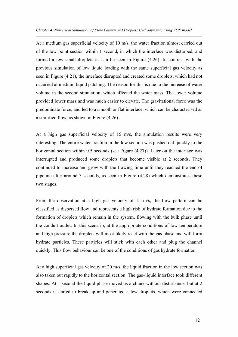
Chapter 4. Numerical Simulation of Flow Pattern and Droplets Hydrodynamic using VOF model ___________________________________________________________________________________
121
At a medium gas superficial velocity of 10 m/s, the water fraction almost carried out
of the low point section within 1 second, in which the interface was disturbed, and
formed a few small droplets as can be seen in Figure (4.26). In contrast with the
previous simulation of low liquid loading with the same superficial gas velocity as
seen in Figure (4.21), the interface disrupted and created some droplets, which had not
occurred at medium liquid patching. The reason for this is due to the increase of water
volume in the second simulation, which affected the water mass. The lower volume
provided lower mass and was much easier to elevate. The gravitational force was the
predominate force, and led to a smooth or flat interface, which can be characterised as
a stratified flow, as shown in Figure (4.26).
At a high gas superficial velocity of 15 m/s, the simulation results were very
interesting. The entire water fraction in the low section was pushed out quickly to the
horizontal section within 0.5 seconds (see Figure (4.27)). Later on the interface was
interrupted and produced some droplets that become visible at 2 seconds. They
continued to increase and grow with the flowing time until they reached the end of
pipeline after around 3 seconds, as seen in Figure (4.28) which demonstrates these
two stages.
From the observation at a high gas velocity of 15 m/s, the flow pattern can be
classified as dispersed flow and represents a high risk of hydrate formation due to the
formation of droplets which remain in the system, flowing with the bulk phase until
the conduit outlet. In this scenario, at the appropriate conditions of low temperature
and high pressure the droplets will most likely react with the gas phase and will form
hydrate particles. These particles will stick with each other and plug the channel
quickly. This flow behaviour can be one of the conditions of gas hydrate formation.
At a high superficial gas velocity of 20 m/s, the liquid fraction in the low section was
also taken out rapidly to the horizontal section. The gas–liquid interface took different
shapes. At 1 second the liquid phase moved as a chunk without disturbance, but at 2
seconds it started to break up and generated a few droplets, which were connected
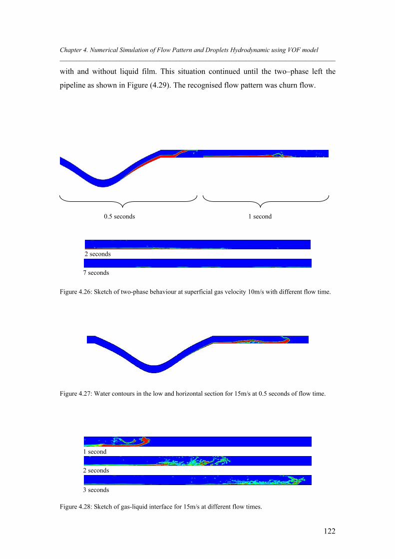
Chapter 4. Numerical Simulation of Flow Pattern and Droplets Hydrodynamic using VOF model ___________________________________________________________________________________
122
with and without liquid film. This situation continued until the two–phase left the
pipeline as shown in Figure (4.29). The recognised flow pattern was churn flow.
2 seconds
7 seconds
Figure 4.26: Sketch of two-phase behaviour at superficial gas velocity 10m/s with different flow time.
Figure 4.27: Water contours in the low and horizontal section for 15m/s at 0.5 seconds of flow time.
1 second
2 seconds
3 seconds Figure 4.28: Sketch of gas-liquid interface for 15m/s at different flow times.
0.5 seconds 1 second
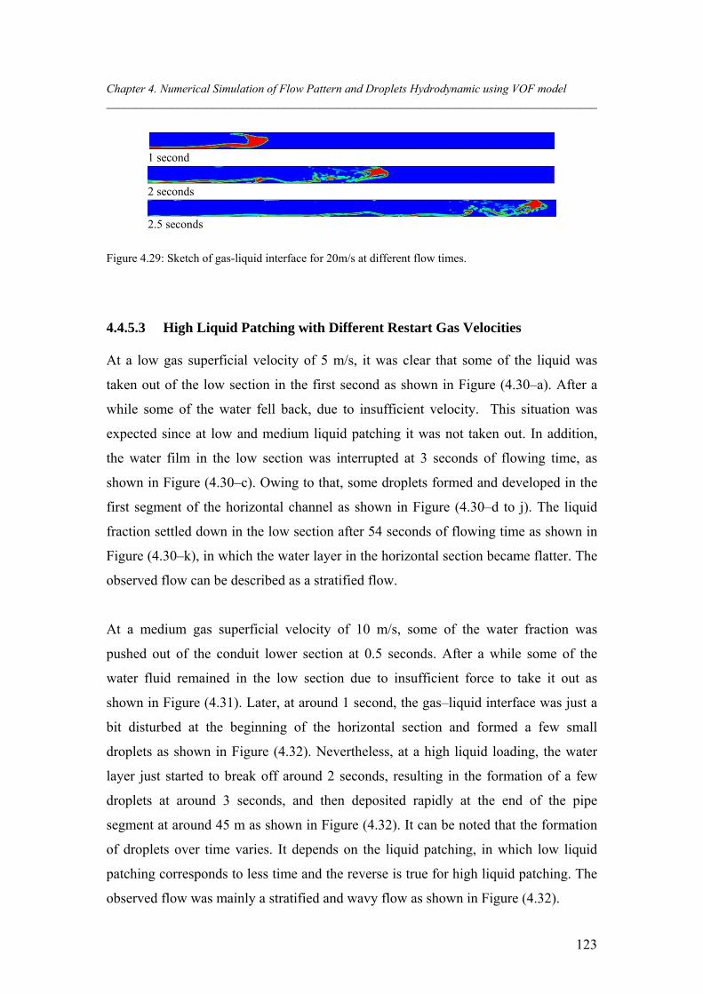
Chapter 4. Numerical Simulation of Flow Pattern and Droplets Hydrodynamic using VOF model ___________________________________________________________________________________
123
1 second
2 seconds
2.5 seconds
Figure 4.29: Sketch of gas-liquid interface for 20m/s at different flow times. 4.4.5.3 High Liquid Patching with Different Restart Gas Velocities
At a low gas superficial velocity of 5 m/s, it was clear that some of the liquid was
taken out of the low section in the first second as shown in Figure (4.30–a). After a
while some of the water fell back, due to insufficient velocity. This situation was
expected since at low and medium liquid patching it was not taken out. In addition,
the water film in the low section was interrupted at 3 seconds of flowing time, as
shown in Figure (4.30–c). Owing to that, some droplets formed and developed in the
first segment of the horizontal channel as shown in Figure (4.30–d to j). The liquid
fraction settled down in the low section after 54 seconds of flowing time as shown in
Figure (4.30–k), in which the water layer in the horizontal section became flatter. The
observed flow can be described as a stratified flow.
At a medium gas superficial velocity of 10 m/s, some of the water fraction was
pushed out of the conduit lower section at 0.5 seconds. After a while some of the
water fluid remained in the low section due to insufficient force to take it out as
shown in Figure (4.31). Later, at around 1 second, the gas–liquid interface was just a
bit disturbed at the beginning of the horizontal section and formed a few small
droplets as shown in Figure (4.32). Nevertheless, at a high liquid loading, the water
layer just started to break off around 2 seconds, resulting in the formation of a few
droplets at around 3 seconds, and then deposited rapidly at the end of the pipe
segment at around 45 m as shown in Figure (4.32). It can be noted that the formation
of droplets over time varies. It depends on the liquid patching, in which low liquid
patching corresponds to less time and the reverse is true for high liquid patching. The
observed flow was mainly a stratified and wavy flow as shown in Figure (4.32).
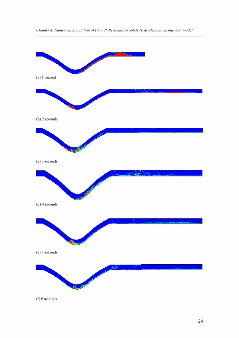
Chapter 4. Numerical Simulation of Flow Pattern and Droplets Hydrodynamic using VOF model ___________________________________________________________________________________
124
(a) 1 second
(b) 2 seconds
(c) 3 seconds
(d) 4 seconds
(e) 5 seconds
(f) 6 seconds
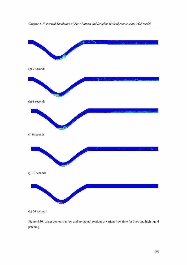
Chapter 4. Numerical Simulation of Flow Pattern and Droplets Hydrodynamic using VOF model ___________________________________________________________________________________
125
(g) 7 seconds
(h) 8 seconds
(i) 9 seconds
(j) 10 seconds
(k) 54 seconds
Figure 4.30: Water contours at low and horizontal sections at variant flow time for 5m/s and high liquid
patching.
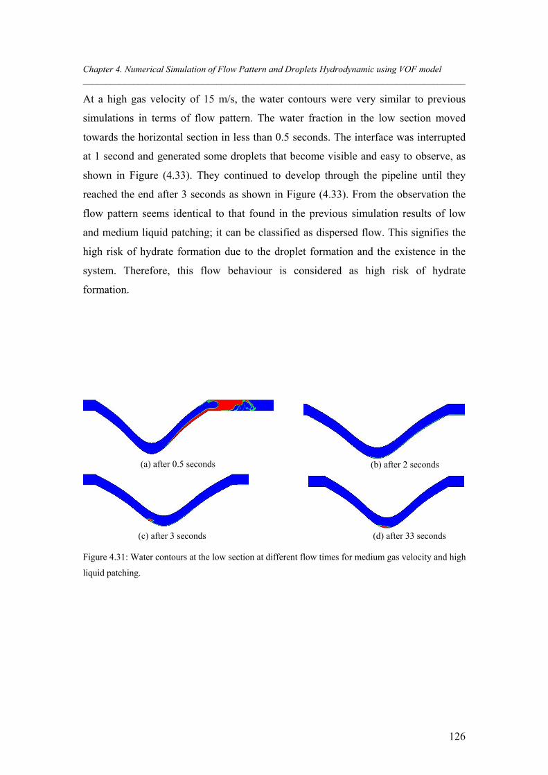
Chapter 4. Numerical Simulation of Flow Pattern and Droplets Hydrodynamic using VOF model ___________________________________________________________________________________
126
At a high gas velocity of 15 m/s, the water contours were very similar to previous
simulations in terms of flow pattern. The water fraction in the low section moved
towards the horizontal section in less than 0.5 seconds. The interface was interrupted
at 1 second and generated some droplets that become visible and easy to observe, as
shown in Figure (4.33). They continued to develop through the pipeline until they
reached the end after 3 seconds as shown in Figure (4.33). From the observation the
flow pattern seems identical to that found in the previous simulation results of low
and medium liquid patching; it can be classified as dispersed flow. This signifies the
high risk of hydrate formation due to the droplet formation and the existence in the
system. Therefore, this flow behaviour is considered as high risk of hydrate
formation.
Figure 4.31: Water contours at the low section at different flow times for medium gas velocity and high
liquid patching.
(a) after 0.5 seconds
(b) after 2 seconds
(c) after 3 seconds
(d) after 33 seconds
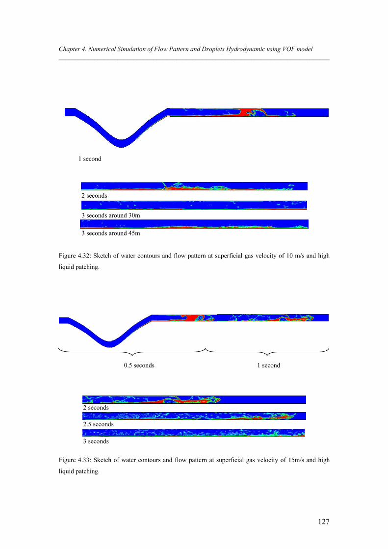
Chapter 4. Numerical Simulation of Flow Pattern and Droplets Hydrodynamic using VOF model ___________________________________________________________________________________
127
1 second
2 seconds
3 seconds around 30m
3 seconds around 45m Figure 4.32: Sketch of water contours and flow pattern at superficial gas velocity of 10 m/s and high
liquid patching.
0.5 seconds 1 second
2 seconds
2.5 seconds
3 seconds
Figure 4.33: Sketch of water contours and flow pattern at superficial gas velocity of 15m/s and high
liquid patching.
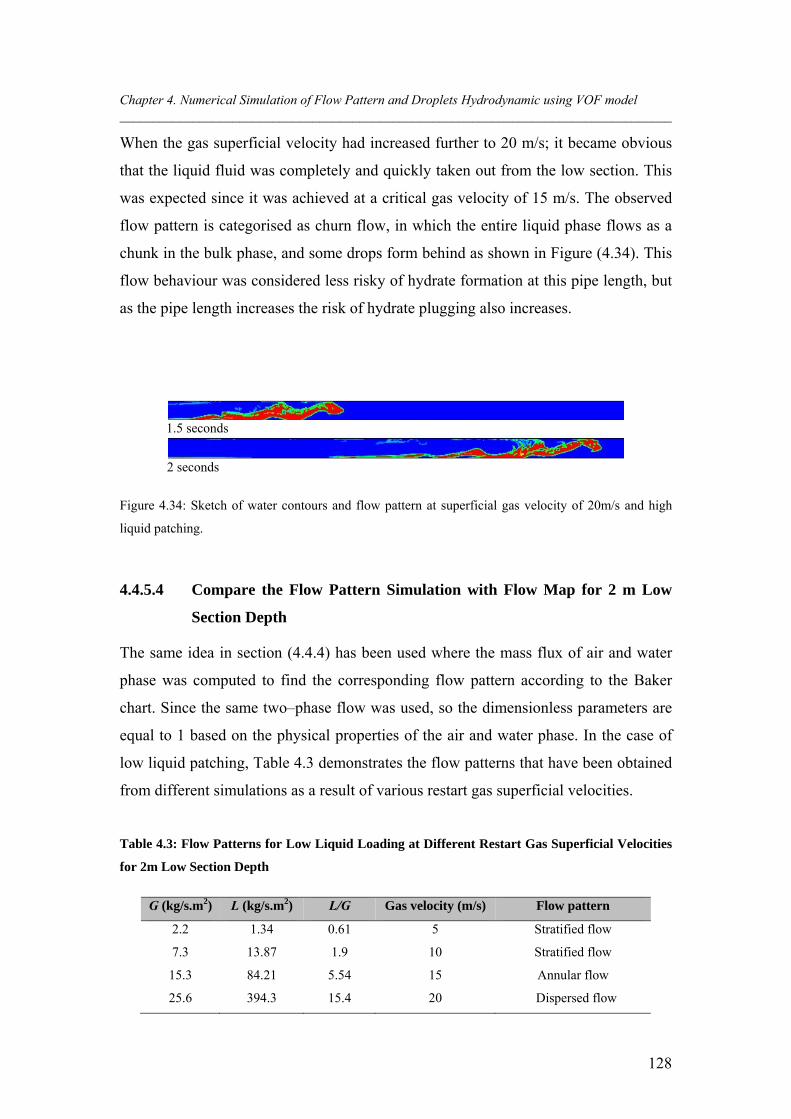
Chapter 4. Numerical Simulation of Flow Pattern and Droplets Hydrodynamic using VOF model ___________________________________________________________________________________
128
When the gas superficial velocity had increased further to 20 m/s; it became obvious
that the liquid fluid was completely and quickly taken out from the low section. This
was expected since it was achieved at a critical gas velocity of 15 m/s. The observed
flow pattern is categorised as churn flow, in which the entire liquid phase flows as a
chunk in the bulk phase, and some drops form behind as shown in Figure (4.34). This
flow behaviour was considered less risky of hydrate formation at this pipe length, but
as the pipe length increases the risk of hydrate plugging also increases.
1.5 seconds
2 seconds
Figure 4.34: Sketch of water contours and flow pattern at superficial gas velocity of 20m/s and high
liquid patching.
4.4.5.4 Compare the Flow Pattern Simulation with Flow Map for 2 m Low
Section Depth
The same idea in section (4.4.4) has been used where the mass flux of air and water
phase was computed to find the corresponding flow pattern according to the Baker
chart. Since the same two–phase flow was used, so the dimensionless parameters are
equal to 1 based on the physical properties of the air and water phase. In the case of
low liquid patching, Table 4.3 demonstrates the flow patterns that have been obtained
from different simulations as a result of various restart gas superficial velocities.
Table 4.3: Flow Patterns for Low Liquid Loading at Different Restart Gas Superficial Velocities
for 2m Low Section Depth
G (kg/s.m2) L (kg/s.m2) L/G Gas velocity (m/s) Flow pattern
2.2 1.34 0.61 5 Stratified flow
7.3 13.87 1.9 10 Stratified flow
15.3 84.21 5.54 15 Annular flow
25.6 394.3 15.4 20 Dispersed flow
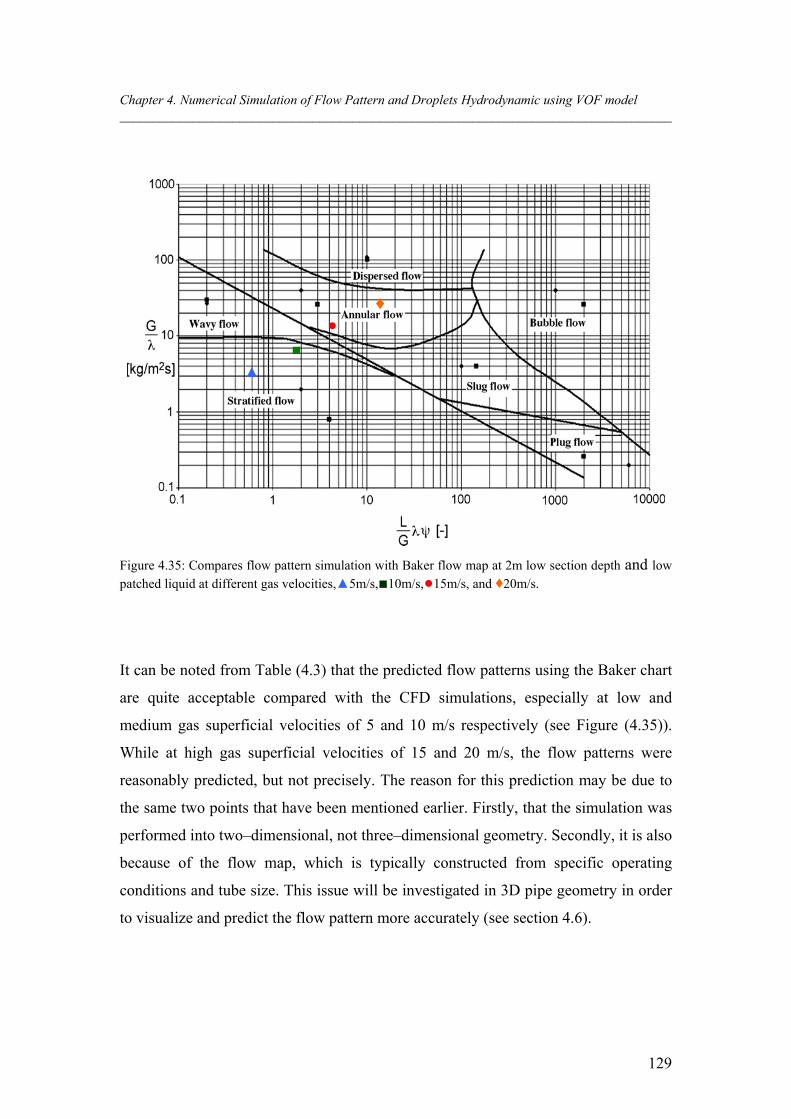
Chapter 4. Numerical Simulation of Flow Pattern and Droplets Hydrodynamic using VOF model ___________________________________________________________________________________
129
Figure 4.35: Compares flow pattern simulation with Baker flow map at 2m low section depth and low patched liquid at different gas velocities,▲5m/s,■10m/s,●15m/s, and ♦20m/s.
It can be noted from Table (4.3) that the predicted flow patterns using the Baker chart
are quite acceptable compared with the CFD simulations, especially at low and
medium gas superficial velocities of 5 and 10 m/s respectively (see Figure (4.35)).
While at high gas superficial velocities of 15 and 20 m/s, the flow patterns were
reasonably predicted, but not precisely. The reason for this prediction may be due to
the same two points that have been mentioned earlier. Firstly, that the simulation was
performed into two–dimensional, not three–dimensional geometry. Secondly, it is also
because of the flow map, which is typically constructed from specific operating
conditions and tube size. This issue will be investigated in 3D pipe geometry in order
to visualize and predict the flow pattern more accurately (see section 4.6).
▲
■
●♦
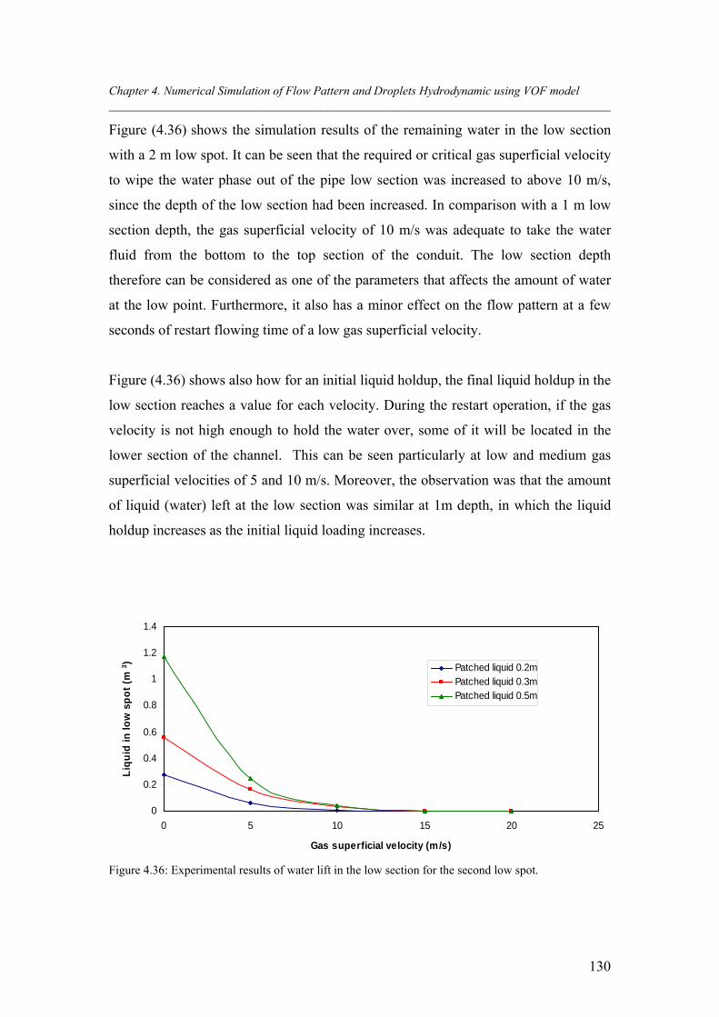
Chapter 4. Numerical Simulation of Flow Pattern and Droplets Hydrodynamic using VOF model ___________________________________________________________________________________
130
Figure (4.36) shows the simulation results of the remaining water in the low section
with a 2 m low spot. It can be seen that the required or critical gas superficial velocity
to wipe the water phase out of the pipe low section was increased to above 10 m/s,
since the depth of the low section had been increased. In comparison with a 1 m low
section depth, the gas superficial velocity of 10 m/s was adequate to take the water
fluid from the bottom to the top section of the conduit. The low section depth
therefore can be considered as one of the parameters that affects the amount of water
at the low point. Furthermore, it also has a minor effect on the flow pattern at a few
seconds of restart flowing time of a low gas superficial velocity.
Figure (4.36) shows also how for an initial liquid holdup, the final liquid holdup in the
low section reaches a value for each velocity. During the restart operation, if the gas
velocity is not high enough to hold the water over, some of it will be located in the
lower section of the channel. This can be seen particularly at low and medium gas
superficial velocities of 5 and 10 m/s. Moreover, the observation was that the amount
of liquid (water) left at the low section was similar at 1m depth, in which the liquid
holdup increases as the initial liquid loading increases.
0
0.2
0.4
0.6
0.8
1
1.2
1.4
0 5 10 15 20 25
Gas superficial velocity (m/s)
Liq
uid
in lo
w s
po
t (m
3)
Patched liquid 0.2mPatched liquid 0.3mPatched liquid 0.5m
Figure 4.36: Experimental results of water lift in the low section for the second low spot.
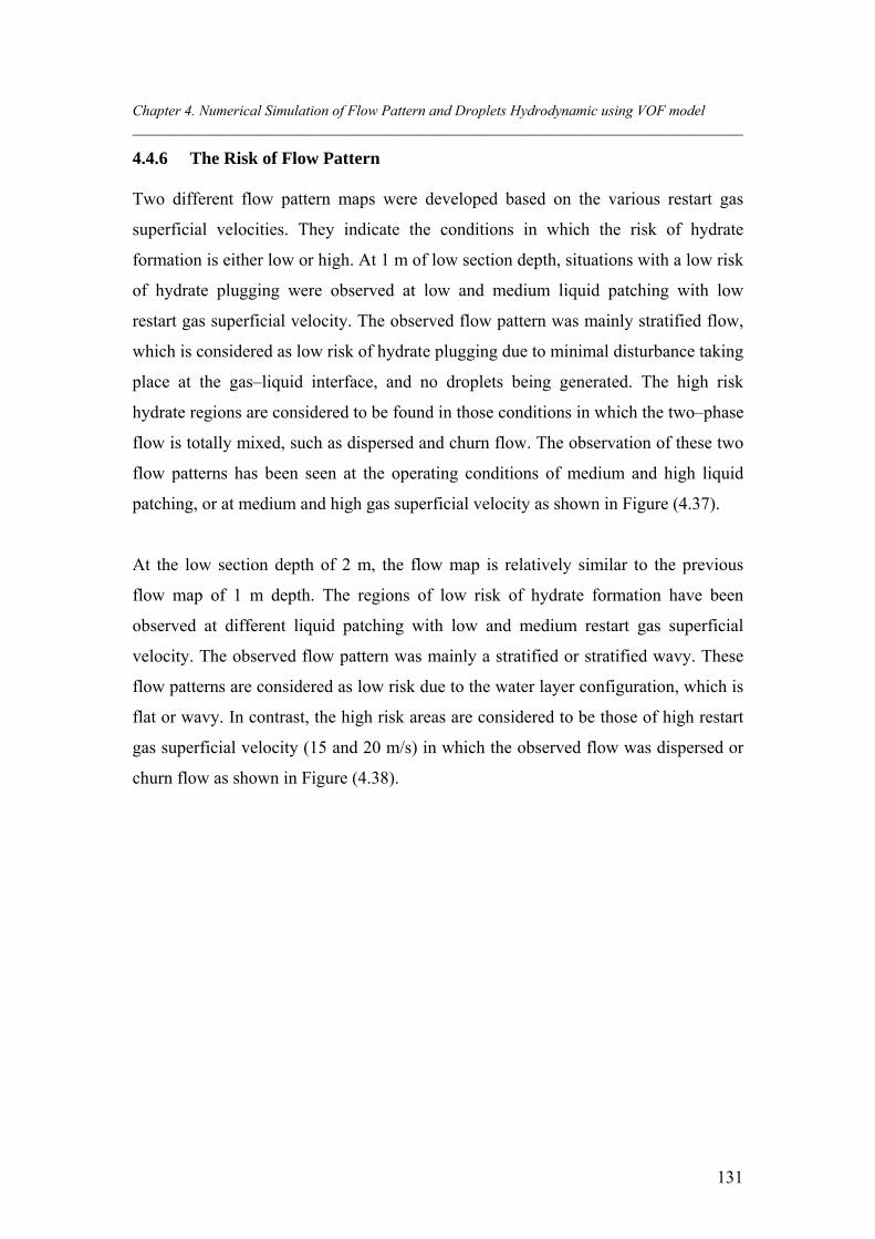
Chapter 4. Numerical Simulation of Flow Pattern and Droplets Hydrodynamic using VOF model ___________________________________________________________________________________
131
4.4.6 The Risk of Flow Pattern
Two different flow pattern maps were developed based on the various restart gas
superficial velocities. They indicate the conditions in which the risk of hydrate
formation is either low or high. At 1 m of low section depth, situations with a low risk
of hydrate plugging were observed at low and medium liquid patching with low
restart gas superficial velocity. The observed flow pattern was mainly stratified flow,
which is considered as low risk of hydrate plugging due to minimal disturbance taking
place at the gas–liquid interface, and no droplets being generated. The high risk
hydrate regions are considered to be found in those conditions in which the two–phase
flow is totally mixed, such as dispersed and churn flow. The observation of these two
flow patterns has been seen at the operating conditions of medium and high liquid
patching, or at medium and high gas superficial velocity as shown in Figure (4.37).
At the low section depth of 2 m, the flow map is relatively similar to the previous
flow map of 1 m depth. The regions of low risk of hydrate formation have been
observed at different liquid patching with low and medium restart gas superficial
velocity. The observed flow pattern was mainly a stratified or stratified wavy. These
flow patterns are considered as low risk due to the water layer configuration, which is
flat or wavy. In contrast, the high risk areas are considered to be those of high restart
gas superficial velocity (15 and 20 m/s) in which the observed flow was dispersed or
churn flow as shown in Figure (4.38).
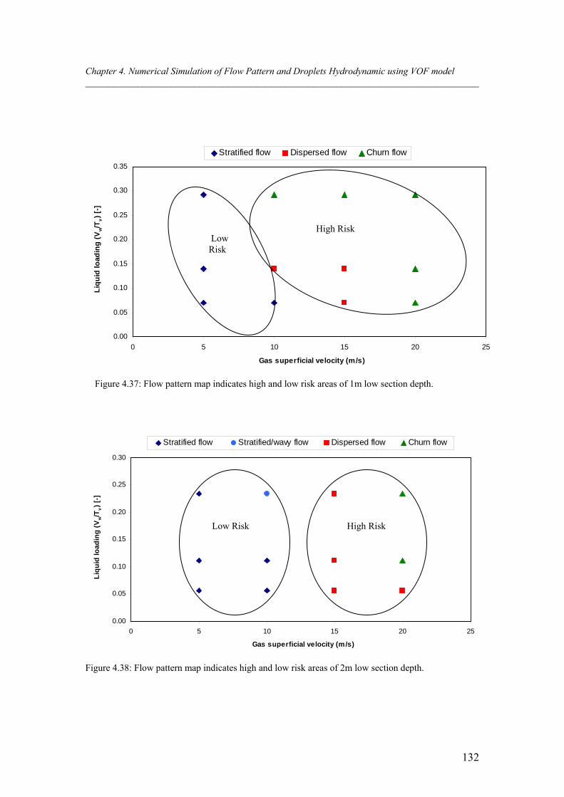
Chapter 4. Numerical Simulation of Flow Pattern and Droplets Hydrodynamic using VOF model ___________________________________________________________________________________
132
0.00
0.05
0.10
0.15
0.20
0.25
0.30
0.35
0 5 10 15 20 25
Gas superficial velocity (m/s)
Liq
uid
load
ing
(V
w/T
v)
[-]
Stratified flow Dispersed flow Churn flow
Figure 4.37: Flow pattern map indicates high and low risk areas of 1m low section depth.
0.00
0.05
0.10
0.15
0.20
0.25
0.30
0 5 10 15 20 25
Gas superficial velocity (m/s)
Liq
uid
load
ing
(V
w/T
v)
[-]
Stratified flow Stratified/wavy flow Dispersed flow Churn flow
Figure 4.38: Flow pattern map indicates high and low risk areas of 2m low section depth.
Low Risk
High Risk
Low Risk
High Risk
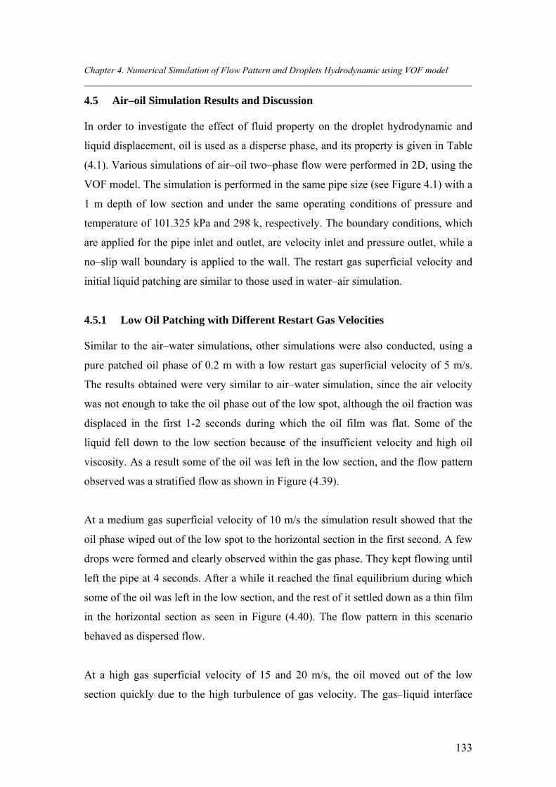
Chapter 4. Numerical Simulation of Flow Pattern and Droplets Hydrodynamic using VOF model ___________________________________________________________________________________
133
4.5 Air–oil Simulation Results and Discussion
In order to investigate the effect of fluid property on the droplet hydrodynamic and
liquid displacement, oil is used as a disperse phase, and its property is given in Table
(4.1). Various simulations of air–oil two–phase flow were performed in 2D, using the
VOF model. The simulation is performed in the same pipe size (see Figure 4.1) with a
1 m depth of low section and under the same operating conditions of pressure and
temperature of 101.325 kPa and 298 k, respectively. The boundary conditions, which
are applied for the pipe inlet and outlet, are velocity inlet and pressure outlet, while a
no–slip wall boundary is applied to the wall. The restart gas superficial velocity and
initial liquid patching are similar to those used in water–air simulation.
4.5.1 Low Oil Patching with Different Restart Gas Velocities
Similar to the air–water simulations, other simulations were also conducted, using a
pure patched oil phase of 0.2 m with a low restart gas superficial velocity of 5 m/s.
The results obtained were very similar to air–water simulation, since the air velocity
was not enough to take the oil phase out of the low spot, although the oil fraction was
displaced in the first 1-2 seconds during which the oil film was flat. Some of the
liquid fell down to the low section because of the insufficient velocity and high oil
viscosity. As a result some of the oil was left in the low section, and the flow pattern
observed was a stratified flow as shown in Figure (4.39).
At a medium gas superficial velocity of 10 m/s the simulation result showed that the
oil phase wiped out of the low spot to the horizontal section in the first second. A few
drops were formed and clearly observed within the gas phase. They kept flowing until
left the pipe at 4 seconds. After a while it reached the final equilibrium during which
some of the oil was left in the low section, and the rest of it settled down as a thin film
in the horizontal section as seen in Figure (4.40). The flow pattern in this scenario
behaved as dispersed flow.
At a high gas superficial velocity of 15 and 20 m/s, the oil moved out of the low
section quickly due to the high turbulence of gas velocity. The gas–liquid interface
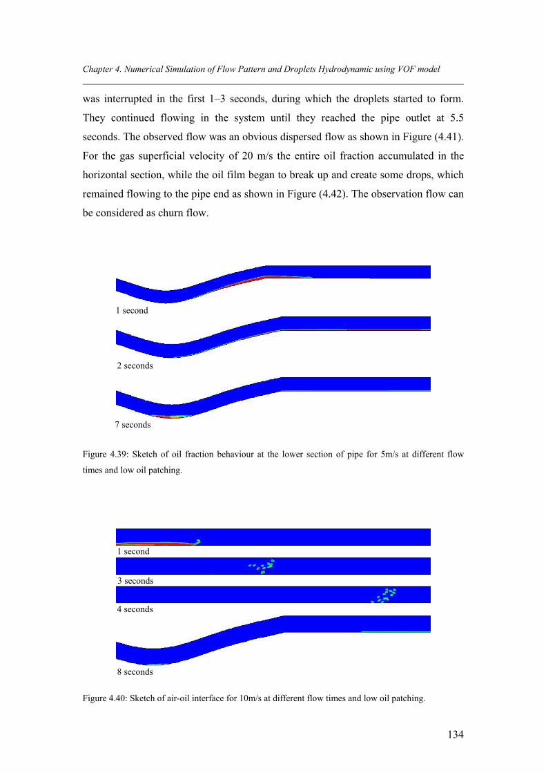
Chapter 4. Numerical Simulation of Flow Pattern and Droplets Hydrodynamic using VOF model ___________________________________________________________________________________
134
was interrupted in the first 1–3 seconds, during which the droplets started to form.
They continued flowing in the system until they reached the pipe outlet at 5.5
seconds. The observed flow was an obvious dispersed flow as shown in Figure (4.41).
For the gas superficial velocity of 20 m/s the entire oil fraction accumulated in the
horizontal section, while the oil film began to break up and create some drops, which
remained flowing to the pipe end as shown in Figure (4.42). The observation flow can
be considered as churn flow.
1 second
2 seconds
7 seconds
Figure 4.39: Sketch of oil fraction behaviour at the lower section of pipe for 5m/s at different flow
times and low oil patching.
1 second
3 seconds
4 seconds
8 seconds
Figure 4.40: Sketch of air-oil interface for 10m/s at different flow times and low oil patching.
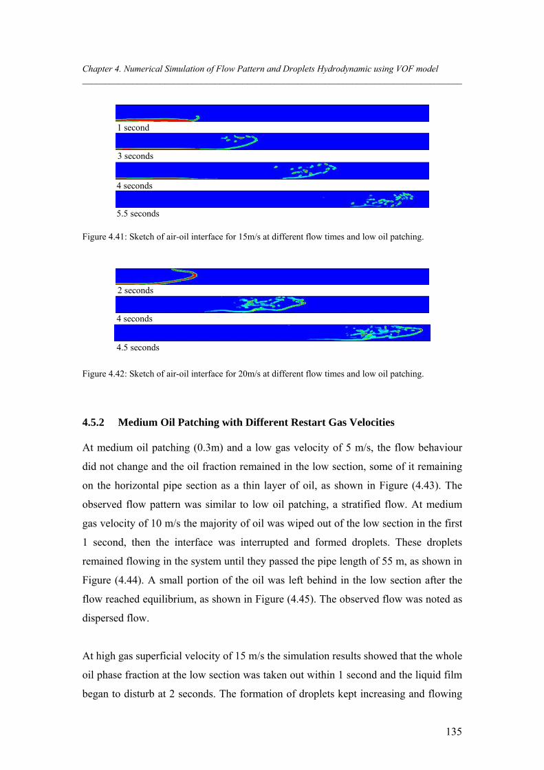
Chapter 4. Numerical Simulation of Flow Pattern and Droplets Hydrodynamic using VOF model ___________________________________________________________________________________
135
1 second
3 seconds
4 seconds
5.5 seconds Figure 4.41: Sketch of air-oil interface for 15m/s at different flow times and low oil patching.
2 seconds
4 seconds
4.5 seconds
Figure 4.42: Sketch of air-oil interface for 20m/s at different flow times and low oil patching.
4.5.2 Medium Oil Patching with Different Restart Gas Velocities
At medium oil patching (0.3m) and a low gas velocity of 5 m/s, the flow behaviour
did not change and the oil fraction remained in the low section, some of it remaining
on the horizontal pipe section as a thin layer of oil, as shown in Figure (4.43). The
observed flow pattern was similar to low oil patching, a stratified flow. At medium
gas velocity of 10 m/s the majority of oil was wiped out of the low section in the first
1 second, then the interface was interrupted and formed droplets. These droplets
remained flowing in the system until they passed the pipe length of 55 m, as shown in
Figure (4.44). A small portion of the oil was left behind in the low section after the
flow reached equilibrium, as shown in Figure (4.45). The observed flow was noted as
dispersed flow.
At high gas superficial velocity of 15 m/s the simulation results showed that the whole
oil phase fraction at the low section was taken out within 1 second and the liquid film
began to disturb at 2 seconds. The formation of droplets kept increasing and flowing
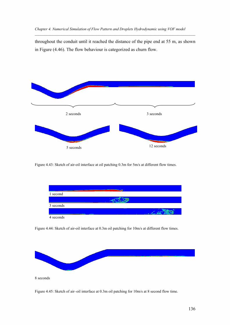
Chapter 4. Numerical Simulation of Flow Pattern and Droplets Hydrodynamic using VOF model ___________________________________________________________________________________
136
throughout the conduit until it reached the distance of the pipe end at 55 m, as shown
in Figure (4.46). The flow behaviour is categorized as churn flow.
2 seconds 3 seconds
5 seconds 12 seconds
Figure 4.43: Sketch of air-oil interface at oil patching 0.3m for 5m/s at different flow times.
1 second
3 seconds
4 seconds
Figure 4.44: Sketch of air-oil interface at 0.3m oil patching for 10m/s at different flow times.
8 seconds
Figure 4.45: Sketch of air–oil interface at 0.3m oil patching for 10m/s at 8 second flow time.
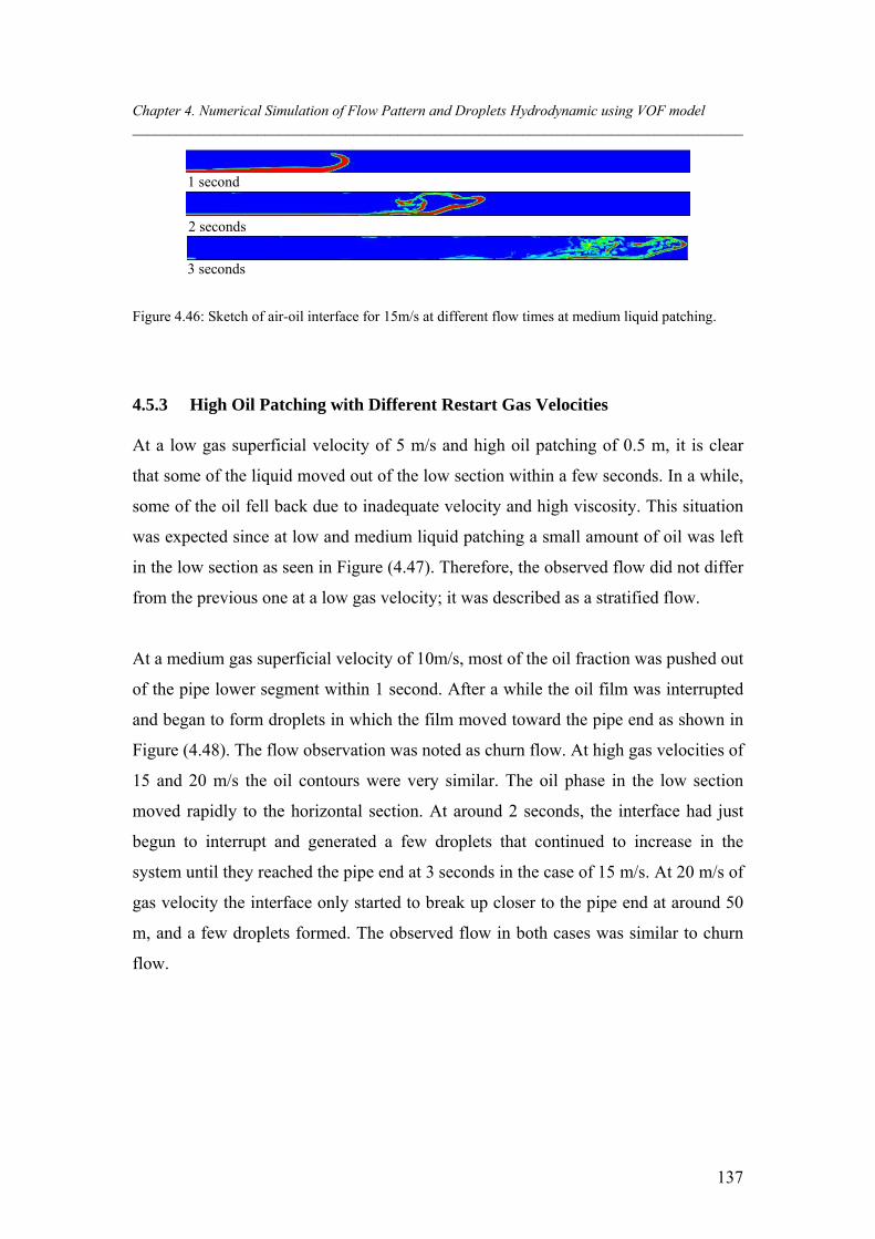
Chapter 4. Numerical Simulation of Flow Pattern and Droplets Hydrodynamic using VOF model ___________________________________________________________________________________
137
1 second
2 seconds
3 seconds
Figure 4.46: Sketch of air-oil interface for 15m/s at different flow times at medium liquid patching.
4.5.3 High Oil Patching with Different Restart Gas Velocities
At a low gas superficial velocity of 5 m/s and high oil patching of 0.5 m, it is clear
that some of the liquid moved out of the low section within a few seconds. In a while,
some of the oil fell back due to inadequate velocity and high viscosity. This situation
was expected since at low and medium liquid patching a small amount of oil was left
in the low section as seen in Figure (4.47). Therefore, the observed flow did not differ
from the previous one at a low gas velocity; it was described as a stratified flow.
At a medium gas superficial velocity of 10m/s, most of the oil fraction was pushed out
of the pipe lower segment within 1 second. After a while the oil film was interrupted
and began to form droplets in which the film moved toward the pipe end as shown in
Figure (4.48). The flow observation was noted as churn flow. At high gas velocities of
15 and 20 m/s the oil contours were very similar. The oil phase in the low section
moved rapidly to the horizontal section. At around 2 seconds, the interface had just
begun to interrupt and generated a few droplets that continued to increase in the
system until they reached the pipe end at 3 seconds in the case of 15 m/s. At 20 m/s of
gas velocity the interface only started to break up closer to the pipe end at around 50
m, and a few droplets formed. The observed flow in both cases was similar to churn
flow.
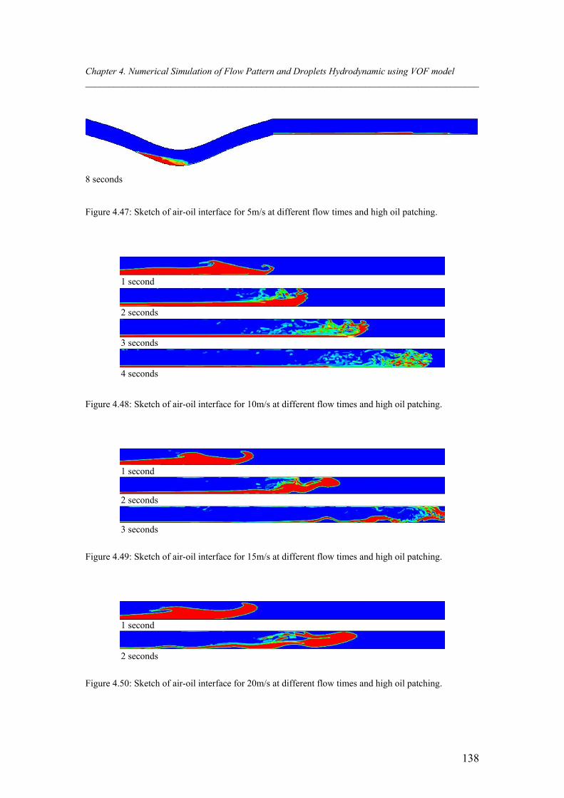
Chapter 4. Numerical Simulation of Flow Pattern and Droplets Hydrodynamic using VOF model ___________________________________________________________________________________
138
8 seconds
Figure 4.47: Sketch of air-oil interface for 5m/s at different flow times and high oil patching.
1 second
2 seconds
3 seconds
4 seconds
Figure 4.48: Sketch of air-oil interface for 10m/s at different flow times and high oil patching.
1 second
2 seconds
3 seconds
Figure 4.49: Sketch of air-oil interface for 15m/s at different flow times and high oil patching.
1 second
2 seconds
Figure 4.50: Sketch of air-oil interface for 20m/s at different flow times and high oil patching.
Chapter 4. Numerical Simulation of Flow Pattern and Droplets Hydrodynamic using VOF model ___________________________________________________________________________________
139
4.5.4 Liquid in the Low Section
In order to study the effect of fluid properties on liquid displacement from the low
section, oil is used with the physical properties as shown in Table (4.1). The result
illustrates that for high oil viscosity, the remaining oil in the low section is
considerably higher than the water fluid. At low gas velocity of 5 m/s and low liquid
patching, the oil had a higher residue of liquid than the water. Even at higher a
velocity of 15 m/s, more liquid (oil) was actually removed, but it was still a small
fraction in the low spot compared with the water as shown in Figure (4.51).
Furthermore, the critical gas velocity in oil simulation was higher than when using
water fluid at low and medium oil patching. A velocity of 15 m/s was insufficient to
wipe the liquid (oil) completely out of the low section whereas 10 m/s had been
enough to take out the water phase, as shown in Figure (4.52). It can be concluded
that fluid viscosity plays a significant role in liquid displacement.
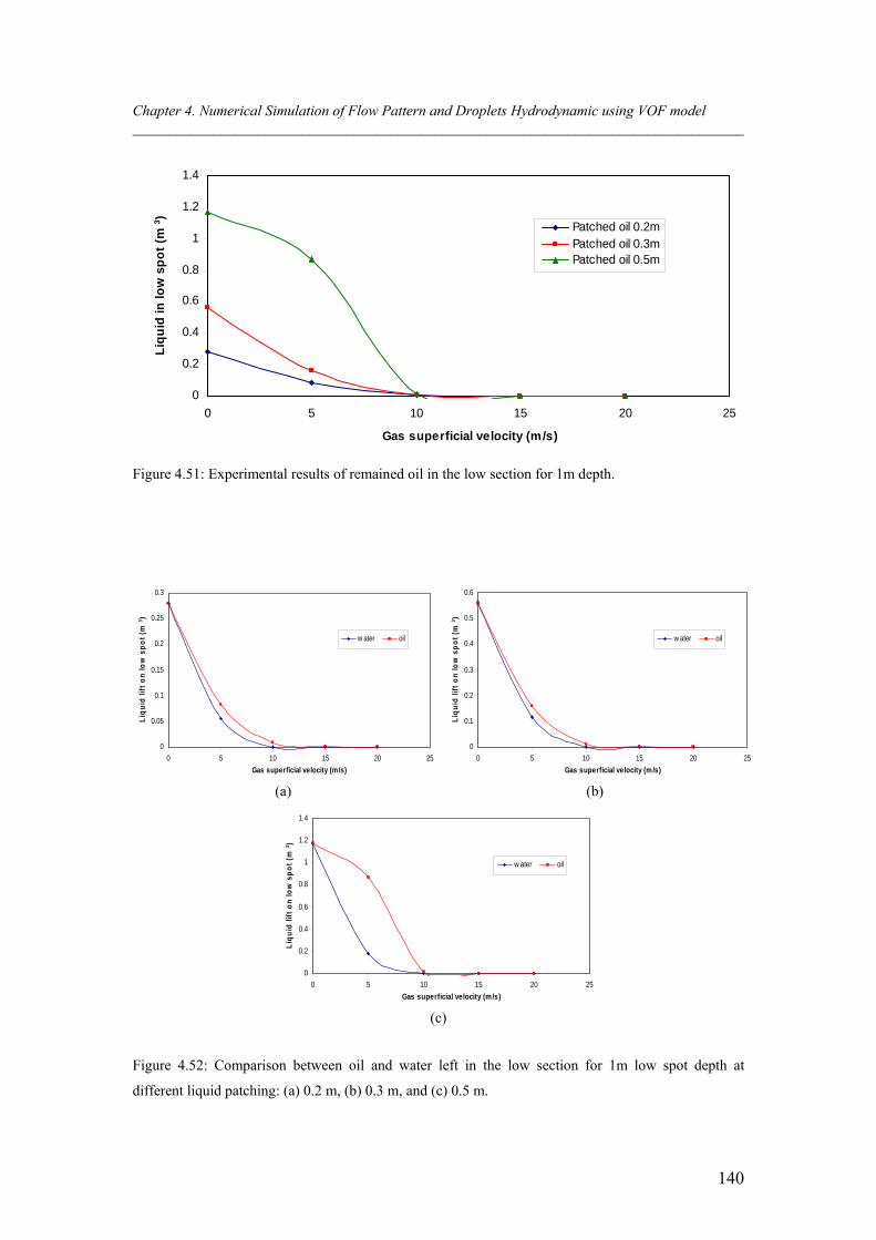
Chapter 4. Numerical Simulation of Flow Pattern and Droplets Hydrodynamic using VOF model ___________________________________________________________________________________
140
0
0.2
0.4
0.6
0.8
1
1.2
1.4
0 5 10 15 20 25
Gas superficial velocity (m/s)
Liq
uid
in lo
w s
po
t (m
3)
Patched oil 0.2mPatched oil 0.3mPatched oil 0.5m
Figure 4.51: Experimental results of remained oil in the low section for 1m depth.
0
0.05
0.1
0.15
0.2
0.25
0.3
0 5 10 15 20 25
Gas superficial velocity (m/s)
Liq
uid
lift
on
low
sp
ot
(m3)
w ater oil
(a)
0
0.1
0.2
0.3
0.4
0.5
0.6
0 5 10 15 20 25
Gas superficial velocity (m/s)
Liq
uid
lift
on
low
sp
ot
(m3)
w ater oil
(b)
0
0.2
0.4
0.6
0.8
1
1.2
1.4
0 5 10 15 20 25
Gas superficial velocity (m/s)
Liq
uid
lift
on
low
sp
ot
(m3)
w ater oil
(c)
Figure 4.52: Comparison between oil and water left in the low section for 1m low spot depth at
different liquid patching: (a) 0.2 m, (b) 0.3 m, and (c) 0.5 m.
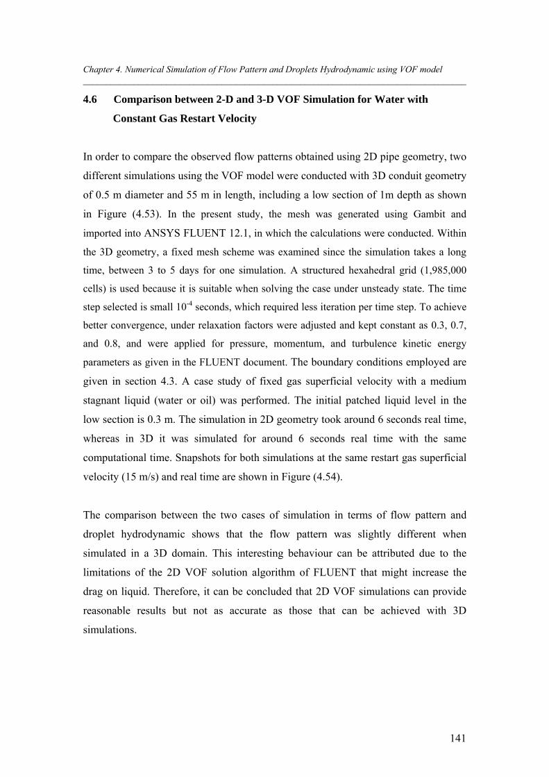
Chapter 4. Numerical Simulation of Flow Pattern and Droplets Hydrodynamic using VOF model ___________________________________________________________________________________
141
4.6 Comparison between 2-D and 3-D VOF Simulation for Water with
Constant Gas Restart Velocity
In order to compare the observed flow patterns obtained using 2D pipe geometry, two
different simulations using the VOF model were conducted with 3D conduit geometry
of 0.5 m diameter and 55 m in length, including a low section of 1m depth as shown
in Figure (4.53). In the present study, the mesh was generated using Gambit and
imported into ANSYS FLUENT 12.1, in which the calculations were conducted. Within
the 3D geometry, a fixed mesh scheme was examined since the simulation takes a long
time, between 3 to 5 days for one simulation. A structured hexahedral grid (1,985,000
cells) is used because it is suitable when solving the case under unsteady state. The time
step selected is small 10-4 seconds, which required less iteration per time step. To achieve
better convergence, under relaxation factors were adjusted and kept constant as 0.3, 0.7,
and 0.8, and were applied for pressure, momentum, and turbulence kinetic energy
parameters as given in the FLUENT document. The boundary conditions employed are
given in section 4.3. A case study of fixed gas superficial velocity with a medium
stagnant liquid (water or oil) was performed. The initial patched liquid level in the
low section is 0.3 m. The simulation in 2D geometry took around 6 seconds real time,
whereas in 3D it was simulated for around 6 seconds real time with the same
computational time. Snapshots for both simulations at the same restart gas superficial
velocity (15 m/s) and real time are shown in Figure (4.54).
The comparison between the two cases of simulation in terms of flow pattern and
droplet hydrodynamic shows that the flow pattern was slightly different when
simulated in a 3D domain. This interesting behaviour can be attributed due to the
limitations of the 2D VOF solution algorithm of FLUENT that might increase the
drag on liquid. Therefore, it can be concluded that 2D VOF simulations can provide
reasonable results but not as accurate as those that can be achieved with 3D
simulations.
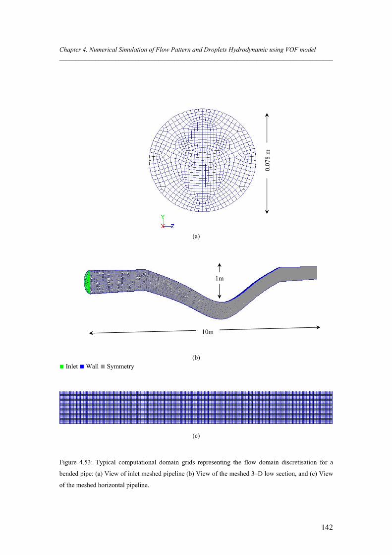
Chapter 4. Numerical Simulation of Flow Pattern and Droplets Hydrodynamic using VOF model ___________________________________________________________________________________
142
(a)
(b) ■ Inlet ■ Wall ■ Symmetry
(c)
Figure 4.53: Typical computational domain grids representing the flow domain discretisation for a
bended pipe: (a) View of inlet meshed pipeline (b) View of the meshed 3–D low section, and (c) View
of the meshed horizontal pipeline.
10 m
0.07
8 m
10m
1m
Chapter 4. Numerical Simulation of Flow Pattern and Droplets Hydrodynamic using VOF model ___________________________________________________________________________________
143
In the three–dimensional simulation of air–water flow, the effect of restart gas
superficial velocity of 15 m/s with the initial patched liquid of 0.3 m on the flow
pattern was quite similar to that observed with 2D simulation, as shown in Figure
(4.54–a). It can also be noted that the water phase was taken out of the low section in
less than 0.5 seconds in the 3D simulation, while in the 2D simulation, it was taken
out in around 1 second. The flow behaviour at 1 second of flowing time was quite
similar, where the liquid film began to lift up, but with slight differences in the
interface configuration. The air–water interface at 2 seconds was also quite similar in
both simulations in which a liquid film was created along the bottom pipe wall, while
the interface configuration was slightly different. In the 3D simulation, the water layer
covered the pipe perimeter, and some drops were located in the core phase. However
in the case of the 2D simulation, the water layer was distributed on the pipe edge, and
some drops flowed in the core phase. Schematically the description of both cases are
shown in Figure (4.54–a).
The predicted flow patterns using the two different dimensions were similarly quite
descriptive. Another simulation was conducted under the same conditions of a restart
gas velocity and low section level, but with high liquid patching of 0.5 m. The flow
pattern observation at 1 second in two and three–dimensional simulations was quite
similar, in which most of the liquid film remained on the bottom pipe wall while some
of it rose up. At 2 seconds of flowing time, the air–water interface began to break off
and produced few drops, whereas the liquid film remained on the bottom tube wall.
The liquid film remained down at 3 seconds of flowing time with more developed
drops. Therefore, the prediction of flow pattern using 2D and 3D simulations was
quite reasonable, but the interface configuration was slightly different as shown
schematically in Figure (4.54–b). In order to verify the flow pattern result, the flow
pattern was obtained using the Baker (1954) flow map. Figure (4.55) shows the flow
pattern obtained from each simulation of 2D and 3D. Clearly the 3D simulation
prediction was much more accurate in comparison to the 2D simulation, which had
provided a reasonable prediction.
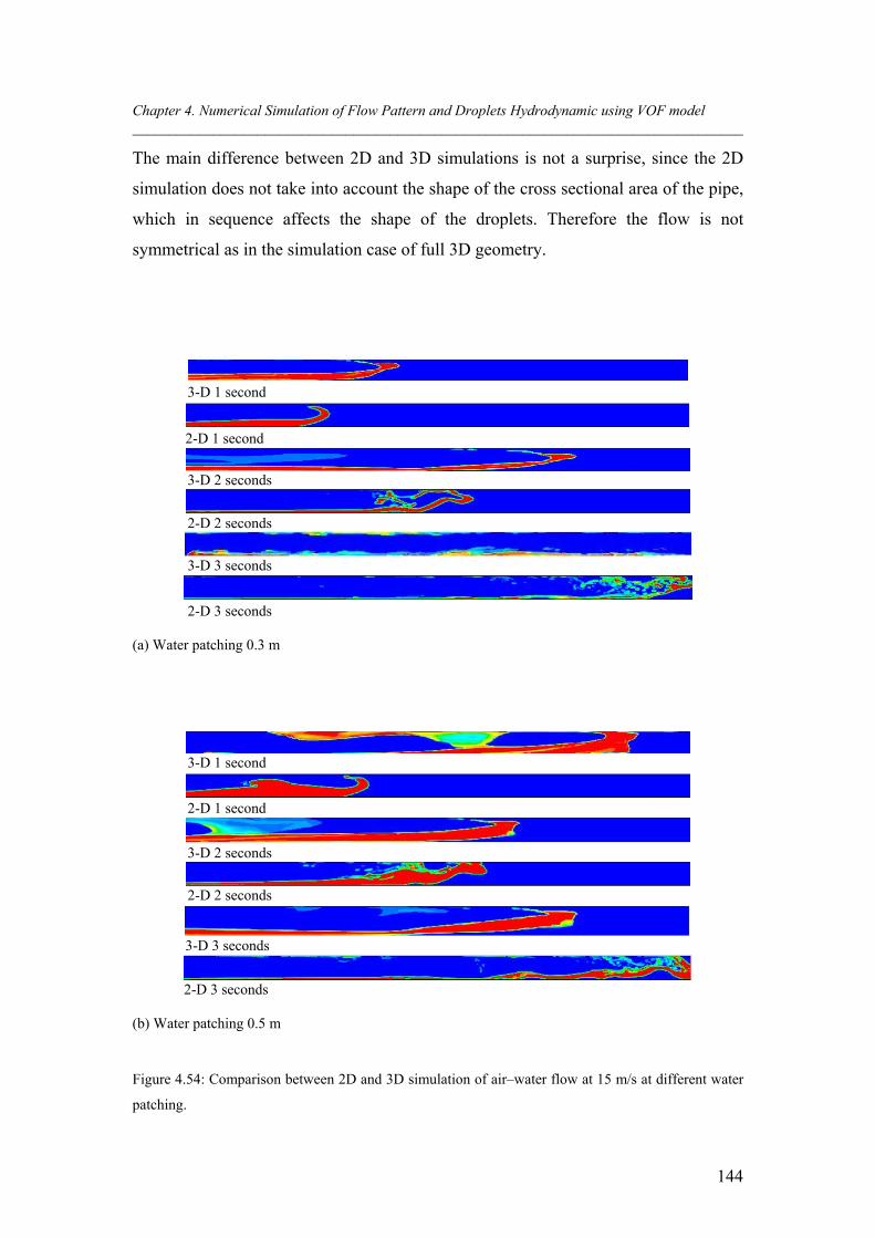
Chapter 4. Numerical Simulation of Flow Pattern and Droplets Hydrodynamic using VOF model ___________________________________________________________________________________
144
The main difference between 2D and 3D simulations is not a surprise, since the 2D
simulation does not take into account the shape of the cross sectional area of the pipe,
which in sequence affects the shape of the droplets. Therefore the flow is not
symmetrical as in the simulation case of full 3D geometry.
3-D 1 second
2-D 1 second
3-D 2 seconds
2-D 2 seconds
3-D 3 seconds
2-D 3 seconds (a) Water patching 0.3 m
3-D 1 second
2-D 1 second
3-D 2 seconds
2-D 2 seconds
3-D 3 seconds
2-D 3 seconds (b) Water patching 0.5 m
Figure 4.54: Comparison between 2D and 3D simulation of air–water flow at 15 m/s at different water
patching.
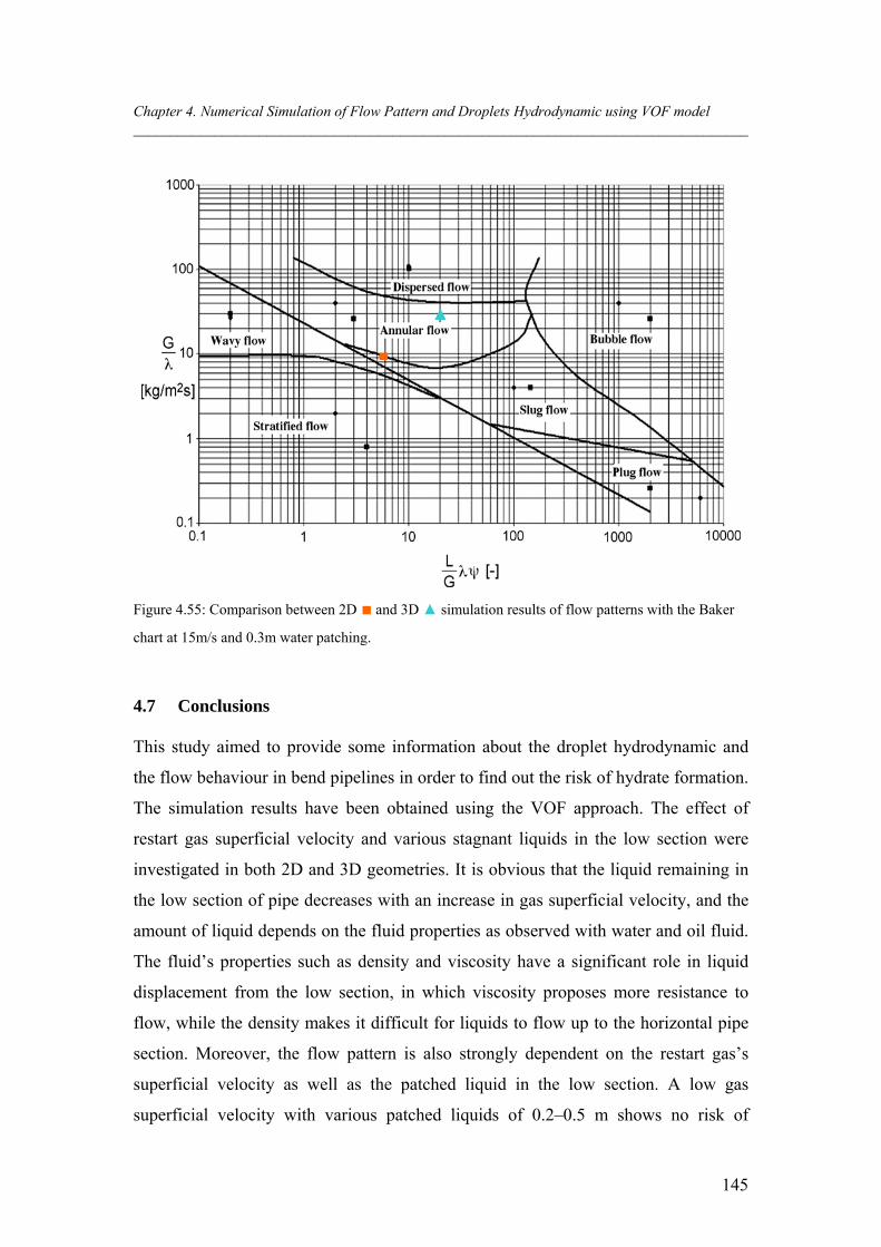
Chapter 4. Numerical Simulation of Flow Pattern and Droplets Hydrodynamic using VOF model ___________________________________________________________________________________
145
Figure 4.55: Comparison between 2D ■ and 3D ▲ simulation results of flow patterns with the Baker
chart at 15m/s and 0.3m water patching.
4.7 Conclusions
This study aimed to provide some information about the droplet hydrodynamic and
the flow behaviour in bend pipelines in order to find out the risk of hydrate formation.
The simulation results have been obtained using the VOF approach. The effect of
restart gas superficial velocity and various stagnant liquids in the low section were
investigated in both 2D and 3D geometries. It is obvious that the liquid remaining in
the low section of pipe decreases with an increase in gas superficial velocity, and the
amount of liquid depends on the fluid properties as observed with water and oil fluid.
The fluid’s properties such as density and viscosity have a significant role in liquid
displacement from the low section, in which viscosity proposes more resistance to
flow, while the density makes it difficult for liquids to flow up to the horizontal pipe
section. Moreover, the flow pattern is also strongly dependent on the restart gas’s
superficial velocity as well as the patched liquid in the low section. A low gas
superficial velocity with various patched liquids of 0.2–0.5 m shows no risk of
▲
■
Chapter 4. Numerical Simulation of Flow Pattern and Droplets Hydrodynamic using VOF model ___________________________________________________________________________________
146
hydrate formation due to the observed flow pattern, and is often a stratified flow.
However as the restart gas velocity is increased, regardless of initial liquid patching,
hydrate formation is more likely to be observed when the flow can be described as
annular, churn or dispersed flow.
The prediction of flow pattern using 3D geometry was more accurate and reliable
compared to the 2D simulation, which provided a reasonable prediction of flow
patterns appearing in the Baker map, specifically at low gas velocity. The results
obtained by the 2D simulation can be considered as an initial start for studying the
flow behaviour at bend pipes. In order to validate the simulation result of the VOF
model more accurately, it is necessary to conduct experimental work to determine the
validity of the model more accurately, instead of using the flow map which is
generated for specific operating conditions and pipe sizes.
4.8 Bibliographies
Fitremann, J. M. (1976). The stability of gas-flow over a stagnant liquid in a pipe and
the onset of slugging. International Journal of Multiphase Flow, 3, 117-122.
Leporcher, E., K. Kinnari, C. Labes-carrier, Ph. Maurel and W. Vandersippe (2002).
Multiphase flow: Can we take advantage of hydrodynamic conditions to avoid
hydrate plugging during deepwater restart operations? The SPE Annual
Technical Conference and Exhibition, San Antonio, Taxes, 29 September-2
October.
Volk, M., E. Delle-Case and A. Coletta (2010). Investigations of flow behavior
formation in well-head jumpers during restart with gas and liquid. Technical
Report, University of Tulsa.
Volk, M., E. Delle-Case and D. Estanga (2007). Risk-based restarts of untreated
subsea oil and gas flowlines in the GoM. Technical Report, University of Tulsa.
“Every reasonable effort has been made to acknowledge the owners of copyright
material. I would be pleased to hear from any copyright owner who has been omitted
or incorrectly acknowledged.”
Chapter 5 Modelling Pressure Drop and Liquid Holdup
with Fixed Droplet Size using Eulerian–
Eulerian Model In this chapter, the three dimensional two–phase flow in a horizontal pipe has been
investigated numerically. The steady state numerical simulations of two–phase gas–
liquid stratified flow in a 0.078 m diameter and 7 m long pipe have been studied using
the commercial CFD package FLUENT 12.1, in conjunction with a multiphase model.
The Eulerian–Eulerian k–ε model was selected to describe the turbulence in
continuous phase. Three fluids were used in this work with air representing the gas
phase and water and oil representing the liquid phase. The purpose is to develop a
model for predicting the pressure drop and liquid holdup at low liquid holdup and also
to examine the behaviour of pressure drop and liquid holdup under different operating
conditions. The numerical results in terms of pressure drop and liquid holdup are
presented and discussed. The predicted results are noted to be in close agreement with
previous results found in the literature. Moreover, it compared well with one of the
existing correlations of two–phase pressure drop and liquid holdup.
Chapter 5.Modelling Pressure Drop and Liquid Holdup with Fixed Drop Size using Eulerian–Eulerian _______________________________________________________________________________________________________
148
5.1 Introduction
The stratified flow regime is frequently encountered in long distance transport
pipelines (e.g. natural gas and oil flows) and in petrochemical and process plants. The
requirements for economic design, optimization of operating conditions and
assessment of safety factors create the need for quantitative information about such
flows. In general, the flow patterns for two–phase flow in a horizontal pipe vary
because of the role played by buoyancy. The prediction of pressure drop and liquid
holdup in two–phase based on the flow conditions has been studied for decades.
Many empirical correlations have been reported in the literature review in Chapter 2.
During the development stage of any gas field many problems have arisen within gas
transmission lines, such as the existence of a small amount of liquid (Cawkwell and
Charles, 1985). Condensation in gas pipelines commonly takes place because of the
variation of temperature and pressure that occurs along the pipeline. The predominant
flow regime in gas condensate pipelines with a small amount of liquid holdup is
Stratified flow. Typically, the existence of liquids in the pipeline is lower than 200
bbl/MMSCFD and corresponding to 1.1% of liquid (Olive et al., 2003).
This amount of liquid can cause several operational problems such as increasing the
pressure that leads to pipe burst and gas hydrate. Such problems can be avoided if an
accurate prediction of two–phase liquid holdup and pressure gradient is obtained.
These two system parameters are significant to pipeline size selection and
downstream facilities. Owing to the inherent complexity of two–phase flows from a
physical and numerical viewpoint, “general” applicable computational fluid dynamics
(CFD) codes are non–existent. The reasons for the lack of fundamental knowledge on
two–phase flows are three–fold:
1. Two-phase flow is a very complex physical phenomenon where many flow
types can occur, and within each flow type several possible flow regimes can
exist (annular, stratified flow, etc.).
Chapter 5.Modelling Pressure Drop and Liquid Holdup with Fixed Drop Size using Eulerian–Eulerian _______________________________________________________________________________________________________
149
2. The complex physical laws and mathematical treatment of phenomena taking
place in the presence of the two–phase (interface dynamics, coalescence,
break–up, drag, etc.) are still largely undeveloped. For instance, there is still
no agreement on the governing equations (Ghorai and Nigam, 2006).
Additionally, proposed constitutive models are empirical, but often lack
experimental validation for the conditions under which they are applied.
3. The numerics for solving the governing equations and closure laws of two–
phase flows are very complicated. Frequently two–phase flows demonstrate
inherent oscillatory behaviour, requiring costly transient solution algorithms.
In spite of the major difficulties mentioned above, significant progress has been made
in different areas of two–phase flow (Ghorai and Nigam, 2006). Many empirical
correlations and phenomenological models have been proposed for the prediction of
stratified gas–liquid flow parameters over the past two decades (Taitel and Dukler,
1976, Hart et al., 1989, Chen et al., 1997, Vlachos et al., 1999, and Fan et al., 2005).
Due to the lack of knowledge about the distribution of wall shear in stratified pipe
flows, expediential recourse is usually made to the relationship established in single–
phase tube flow, with a resulting loss in the accuracy of the calculation.
Computational fluid dynamics (CFD) techniques have been applied to the calculation
of the stratified pipe flows.
One of the early CFD models of turbulent stratified flow in a horizontal conduit was
presented by Shoham and Taitel, 1984. Solutions for turbulent liquid flows were
obtained in horizontal and slightly inclined pipes of 25.4 mm diameter. Issa (1988)
numerically simulated the stratified gas–liquid two–phase flow in pipes, using the
standard k–ε turbulence model with the wall functions for each phase. Newton and
Behnia (1988) obtained more satisfactory solutions for stratified pipe flow using a low
Reynolds number turbulent model instead of wall functions.
In the present chapter, the CFD code ANSYS FLUENT 12.1 is used to develop a
model for pressure drop and liquid holdup at low liquid loading and to understand the
Chapter 5.Modelling Pressure Drop and Liquid Holdup with Fixed Drop Size using Eulerian–Eulerian _______________________________________________________________________________________________________
150
pressure drop behaviour of gas–liquid two–phase in horizontal pipelines as well as the
liquid holdup, which strongly influences the pressure drop in the system.
5.2 Development of Multiphase Flow Model
The gas–liquid two–phase flow in a pipeline is a complex multiphase and turbulent
flow governed by mass and momentum conservation, turbulence transport, and
interphase momentum transfer. Therefore, the following assumptions were made in
developing a theoretical model that characterizes the gas–liquid (air–water/or oil)
multiphase process.
I. The two–phase pipeline system temperature is constant at an ambient
temperature of 25 oC, and the outlet pressure is at 1 atm, in which each phase
is isothermal and incompressible.
II. The two–phase flow is assumed to be a stratified flow based on the two–phase
superficial velocity and flow map (as shown in Figure 5.7), in which the gas
phase is treated as the primary phase, while the liquid phase is treated as the
secondary phase.
III. All droplets are assumed to be uniform in size and exhibit a spherical shape,
and droplet coalescence and breakage are assumed to be negligible in this case
study.
IV. Different phases move at different velocities which are identified here as
physical velocity, and is calculated based on the volume fraction of each
phase.
V. The drag force from the gas phase acting on the water droplets is included in
the interphase momentum exchange.
Chapter 5.Modelling Pressure Drop and Liquid Holdup with Fixed Drop Size using Eulerian–Eulerian _______________________________________________________________________________________________________
151
VI. No external body force and virtual mass force are included in this simulation,
but the effect of lift force on the droplet is assumed constant at 0.005 in order
to math the experiment data.
VII. Each turbulence model is only applicable to the mixture in which two phases
share the same turbulence quantities (e.g. k, ε).
The constant lift coefficient is by definition, a single value which can be either
positive or negative. Therefore, it does not vary with local hydrodynamic conditions
or other flow properties. Several gas–liquid studies in the past have successfully fitted
both positive and negative constant lift coefficients to experimental data (Wang et al.,
1986; Bel Fdhila, 1991; Lahey et al., 1993; Grossetete, 1995). For instance, for fully
developed gas–liquid flows in a vertical pipe, the values of constant lift coefficient
that resulted in a good fit to the experimental data were found to be in the range 0.01
≤ CL ≤ 0.15 (Wang et al., 1986; Lahey et al., 1993).
Therefore, many investigators found it necessary to use lift coefficient values that are
significantly less than the inviscid value of 0.5, and in some cases even negative, in
order to match their experimental data. Therefore, the value of 0.005 was a good
match with the experimental data.
5.3 Domain Description
In order to study the validity of the Eulerian–Eulerian approach for modeling the
pressure drop and liquid holdup in a horizontal pipeline, 3D simulations were
performed with air and water as continuous and dispersed phases, respectively. The
geometry consisted of a straight horizontal pipe 78 mm in diameter. This value of the
pipe diameter was chosen to be consistent with that normally used by Badie et al.
(2000) for studying the pressure drop and liquid holdup. A pipe length of 7 m was
used with three surface boundaries: inlet, outlet, and wall. The actual pipe length that
was used in the experiment is 20 m, but 7 m was chosen because it was sufficient to
obtain a fully developed velocity profile.
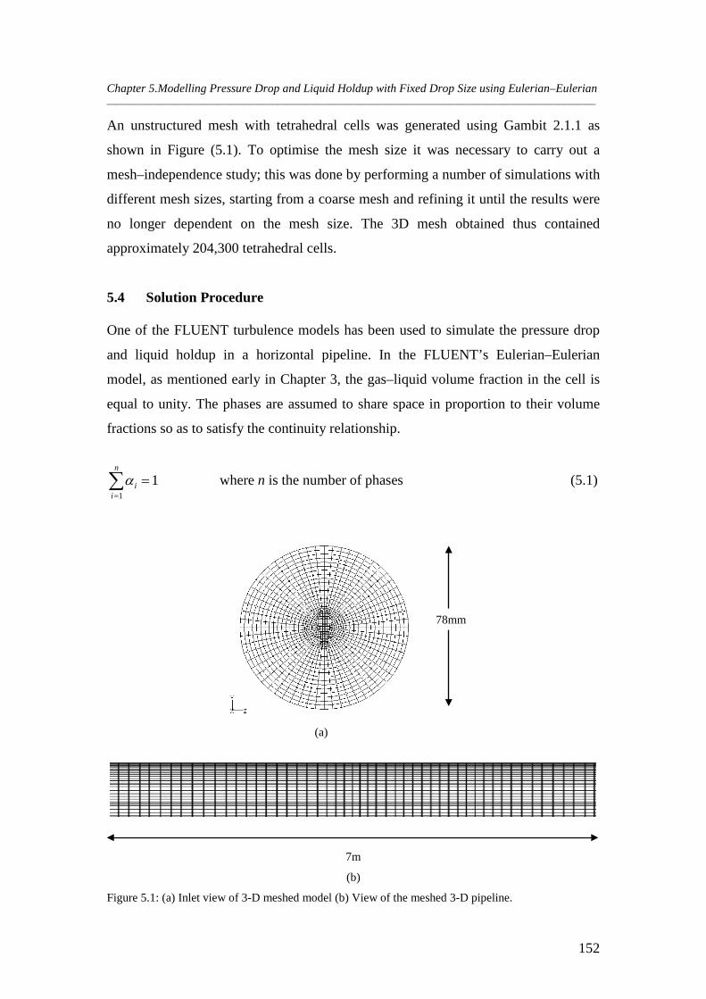
Chapter 5.Modelling Pressure Drop and Liquid Holdup with Fixed Drop Size using Eulerian–Eulerian _______________________________________________________________________________________________________
152
An unstructured mesh with tetrahedral cells was generated using Gambit 2.1.1 as
shown in Figure (5.1). To optimise the mesh size it was necessary to carry out a
mesh–independence study; this was done by performing a number of simulations with
different mesh sizes, starting from a coarse mesh and refining it until the results were
no longer dependent on the mesh size. The 3D mesh obtained thus contained
approximately 204,300 tetrahedral cells.
5.4 Solution Procedure
One of the FLUENT turbulence models has been used to simulate the pressure drop
and liquid holdup in a horizontal pipeline. In the FLUENT’s Eulerian–Eulerian
model, as mentioned early in Chapter 3, the gas–liquid volume fraction in the cell is
equal to unity. The phases are assumed to share space in proportion to their volume
fractions so as to satisfy the continuity relationship.
11
=∑=
n
iiα where n is the number of phases (5.1)
(a)
7m
(b)
Figure 5.1: (a) Inlet view of 3-D meshed model (b) View of the meshed 3-D pipeline.
78mm
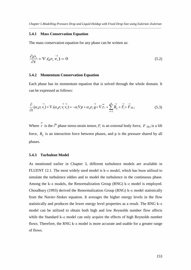
Chapter 5.Modelling Pressure Drop and Liquid Holdup with Fixed Drop Size using Eulerian–Eulerian _______________________________________________________________________________________________________
153
5.4.1 Mass Conservation Equation
The mass conservation equation for any phase can be written as:
0).( =∇+∂
∂ →
iii v
tρρ (5.2)
5.4.2 Momentum Conservation Equation
Each phase has its momentum equation that is solved through the whole domain. It
can be expressed as follows:
ilifti
m
nijiiiiiiiiiii FFRgpvvv
t,
1.).()(
→→
=
→→→→→
+++∇++∇−=∇+∂∂ ∑τρααραρα (5.3)
Where τ is the ith phase stress-strain tensor, iF is an external body force, F lift,i is a lift
force, ijR is an interaction force between phases, and p is the pressure shared by all
phases.
5.4.3 Turbulent Model
As mentioned earlier in Chapter 3, different turbulence models are available in
FLUENT 12.1. The most widely used model is k–ε model, which has been utilised to
simulate the turbulence eddies and to model the turbulence in the continuous phase.
Among the k–ε models, the Renormalization Group (RNG) k–ε model is employed.
Choudhury (1993) derived the Renormalization Group (RNG) k–ε model statistically
from the Navier–Stokes equation. It averages the higher energy levels in the flow
statistically and produces the lower energy level properties as a result. The RNG k–ε
model can be utilized to obtain both high and low Reynolds number flow affects
while the Standard k–ε model can only acquire the effects of high Reynolds number
flows. Therefore, the RNG k–ε model is more accurate and usable for a greater range
of flows.
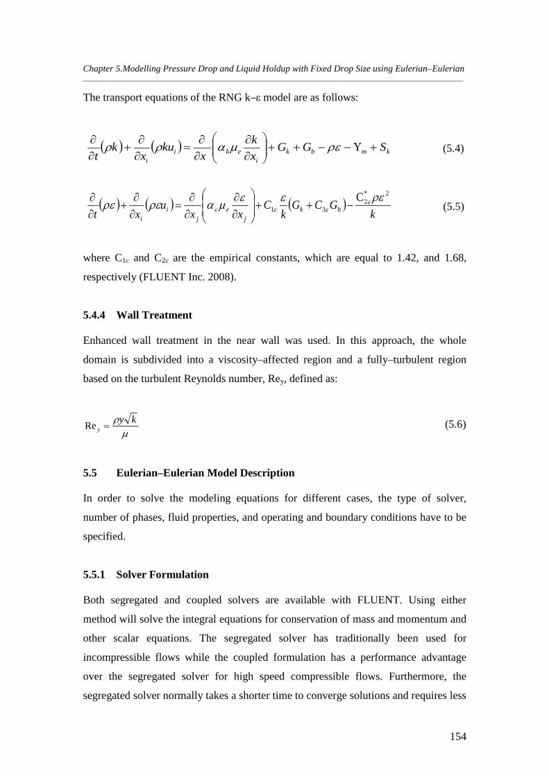
Chapter 5.Modelling Pressure Drop and Liquid Holdup with Fixed Drop Size using Eulerian–Eulerian _______________________________________________________________________________________________________
154
The transport equations of the RNG k–ε model are as follows:
( ) ( ) kmbki
ekii
SGGxk
xku
xk
t+Υ−−++
∂∂
∂∂
=∂∂
+∂∂ ρεµαρρ (5.4)
( ) ( ) ( )k
GCGk
Cxx
uxt bk
je
ji
i
2*2
31C ρεεεµαρερε ε
εεε −++
∂∂
∂∂
=∂∂
+∂∂
(5.5)
where C1ε and C2ε are the empirical constants, which are equal to 1.42, and 1.68,
respectively (FLUENT Inc. 2008).
5.4.4 Wall Treatment
Enhanced wall treatment in the near wall was used. In this approach, the whole
domain is subdivided into a viscosity–affected region and a fully–turbulent region
based on the turbulent Reynolds number, Rey, defined as:
µρ ky
y =Re (5.6)
5.5 Eulerian–Eulerian Model Description
In order to solve the modeling equations for different cases, the type of solver,
number of phases, fluid properties, and operating and boundary conditions have to be
specified.
5.5.1 Solver Formulation
Both segregated and coupled solvers are available with FLUENT. Using either
method will solve the integral equations for conservation of mass and momentum and
other scalar equations. The segregated solver has traditionally been used for
incompressible flows while the coupled formulation has a performance advantage
over the segregated solver for high speed compressible flows. Furthermore, the
segregated solver normally takes a shorter time to converge solutions and requires less
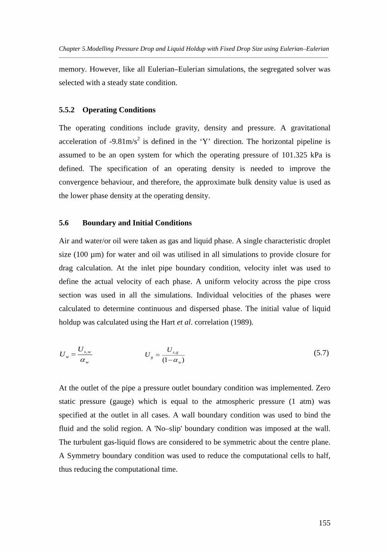
Chapter 5.Modelling Pressure Drop and Liquid Holdup with Fixed Drop Size using Eulerian–Eulerian _______________________________________________________________________________________________________
155
memory. However, like all Eulerian–Eulerian simulations, the segregated solver was
selected with a steady state condition.
5.5.2 Operating Conditions
The operating conditions include gravity, density and pressure. A gravitational
acceleration of -9.81m/s2 is defined in the ‘Y’ direction. The horizontal pipeline is
assumed to be an open system for which the operating pressure of 101.325 kPa is
defined. The specification of an operating density is needed to improve the
convergence behaviour, and therefore, the approximate bulk density value is used as
the lower phase density at the operating density.
5.6 Boundary and Initial Conditions
Air and water/or oil were taken as gas and liquid phase. A single characteristic droplet
size (100 µm) for water and oil was utilised in all simulations to provide closure for
drag calculation. At the inlet pipe boundary condition, velocity inlet was used to
define the actual velocity of each phase. A uniform velocity across the pipe cross
section was used in all the simulations. Individual velocities of the phases were
calculated to determine continuous and dispersed phase. The initial value of liquid
holdup was calculated using the Hart et al. correlation (1989).
w
wsw
UU
α,=
)1(,
w
gsg
UU
α−= (5.7)
At the outlet of the pipe a pressure outlet boundary condition was implemented. Zero
static pressure (gauge) which is equal to the atmospheric pressure (1 atm) was
specified at the outlet in all cases. A wall boundary condition was used to bind the
fluid and the solid region. A 'No–slip' boundary condition was imposed at the wall.
The turbulent gas-liquid flows are considered to be symmetric about the centre plane.
A Symmetry boundary condition was used to reduce the computational cells to half,
thus reducing the computational time.
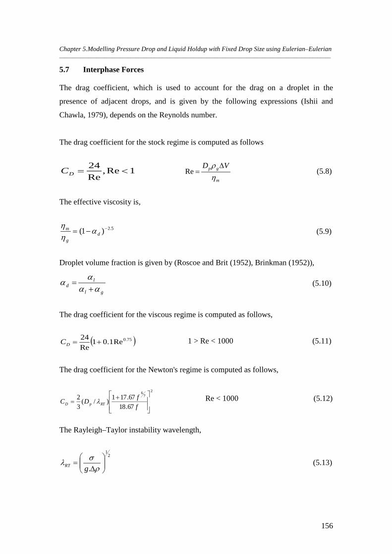
Chapter 5.Modelling Pressure Drop and Liquid Holdup with Fixed Drop Size using Eulerian–Eulerian _______________________________________________________________________________________________________
156
5.7 Interphase Forces
The drag coefficient, which is used to account for the drag on a droplet in the
presence of adjacent drops, and is given by the following expressions (Ishii and
Chawla, 1979), depends on the Reynolds number.
The drag coefficient for the stock regime is computed as follows
1Re,Re24
<=DC m
gp VDηρ ∆
=Re (5.8)
The effective viscosity is,
5.2)1( −−= d
g
m αηη
(5.9)
Droplet volume fraction is given by (Roscoe and Brit (1952), Brinkman (1952)),
gl
ld αα
αα+
= (5.10)
The drag coefficient for the viscous regime is computed as follows,
( )75.0Re1.01Re24
+=DC 1 > Re < 1000 (5.11)
The drag coefficient for the Newton's regime is computed as follows,
2
76
67.1867.171)/(
32
+=
ffDC RTpD λ Re < 1000 (5.12)
The Rayleigh–Taylor instability wavelength,
2
1
.
∆
=ρ
σλgRT (5.13)
Chapter 5.Modelling Pressure Drop and Liquid Holdup with Fixed Drop Size using Eulerian–Eulerian _______________________________________________________________________________________________________
157
5.8 Numerical Technique
All of the Eulerian–Eulerian simulations were carried out with two different phase
flows, such as air–water and air–oil where the gas and liquid are taken as primary and
secondary phases, respectively. All of the equations of two–phase 3D turbulence flow
were solved in each cell of the computational domain. In the present Eulerian–
Eulerian model, turbulence was modeled using k–ε model. A renormalization group
of k–ε (RNG k–ε) was used while the enhanced wall treatment functions proposed by
Kader (1981) were used to specify the wall boundary conditions.
All model equations were solved in a segregated, iterative fashion. Calculations were
performed in a time dependent mode and a first order upwind scheme was used for
the discretisation of momentum, volume fraction, k, and ε for a few iterations, and
then was switched to second order for all of them except volume fraction to Quick,
whereas a phase–coupled SIMPLE algorithm was used for pressure velocity coupling.
Under relaxation factors used for pressure and momentum were 0.3 and 0.05
respectively. The same time step of 0.001 seconds was used throughout the
simulation. For turbulence parameters, intensity and hydraulic diameter specifications
were found to be quite useful. The convergence criteria for residuals were set to
1×10⁻⁴ for each time step.
In order to reduce computational time for these memory intensive simulation studies
all simulations were performed on high speed clusters, which includes 8 processors.
Simulations were performed until a fully developed flow field was ensured by
examining the overall mass balance and time history of the relevant flow variable.
5.9 Validation of CFD Model
To achieve validation of the Eulerian–Eulerian model used in this study the pressure
drop and liquid holdup were compared with the experimental data for a similar
horizontal pipeline specification (Badie et al., 2000). The objective here was to
attempt and validate the CFD model as much as possible so as to establish confidence
in the numerical results. The various stages of the validation process are described
below.
Chapter 5.Modelling Pressure Drop and Liquid Holdup with Fixed Drop Size using Eulerian–Eulerian _______________________________________________________________________________________________________
158
5.9.1 Examination of Turbulence Models
Several turbulence models were available for utilization. Each turbulence model has
advantages, disadvantages, limitations, and appropriate flow regimes. A large family
of turbulence models exists in the literature, yet there are no quantitative guidelines
for choosing an appropriate turbulence model for a multiphase flow.
This section concentrates on an assessment of three turbulence models, which are
standard k–ε, RNG k–ε, and realizable k–ε. The model tests were conducted in a
horizontal pipe having an internal diameter of 0.078 m and a length of 7 m. Prior to
examining each turbulence model, the standard k–ε, RNG k–ε, and realizable k–ε
models were chosen for a grid independent test.
The following Figures (5.2 and 5.3), illustrate the relationship between the pressure
gradient and liquid holdup against superficial water velocity at constant droplet size
and superficial air velocity of 100 µm and 20 m/s, respectively. It can be seen that
RNG k–ε model had close agreement with the experimental data in terms of pressure
gradient and liquid holdup, and had less percentage of error. Therefore, this model has
been chosen for further sensitivity analysis.
5.9.2 Grid–independent Test
The aim of the grid–independent test was to verify the minimum grid resolution
required to generate a solution that is independent of the grid used. In this test, the
initial value of liquid volume fraction was calculated using the Hart et al. (1989)
correlation. The droplet diameter was constant at 1×10⁻⁴ m, and three different mesh
sizes were used for grid generation. These were 110,330, 204,300, and 401,200.
Table (5.1) shows a comparison between three CFD turbulence models with respect to
the experimental data in which the pressure gradient was chosen at a constant
superficial gas and liquid velocity. The CFD pressure gradient decreases as the grids
become finer. The errors (δ) further indicates that the mesh cell number of 204,300 is
insignificant compared with other two–mesh sizes of 110,330 and 401,200
respectively. In general, a total of 204,300 cells are acceptable for the pipe meshing.
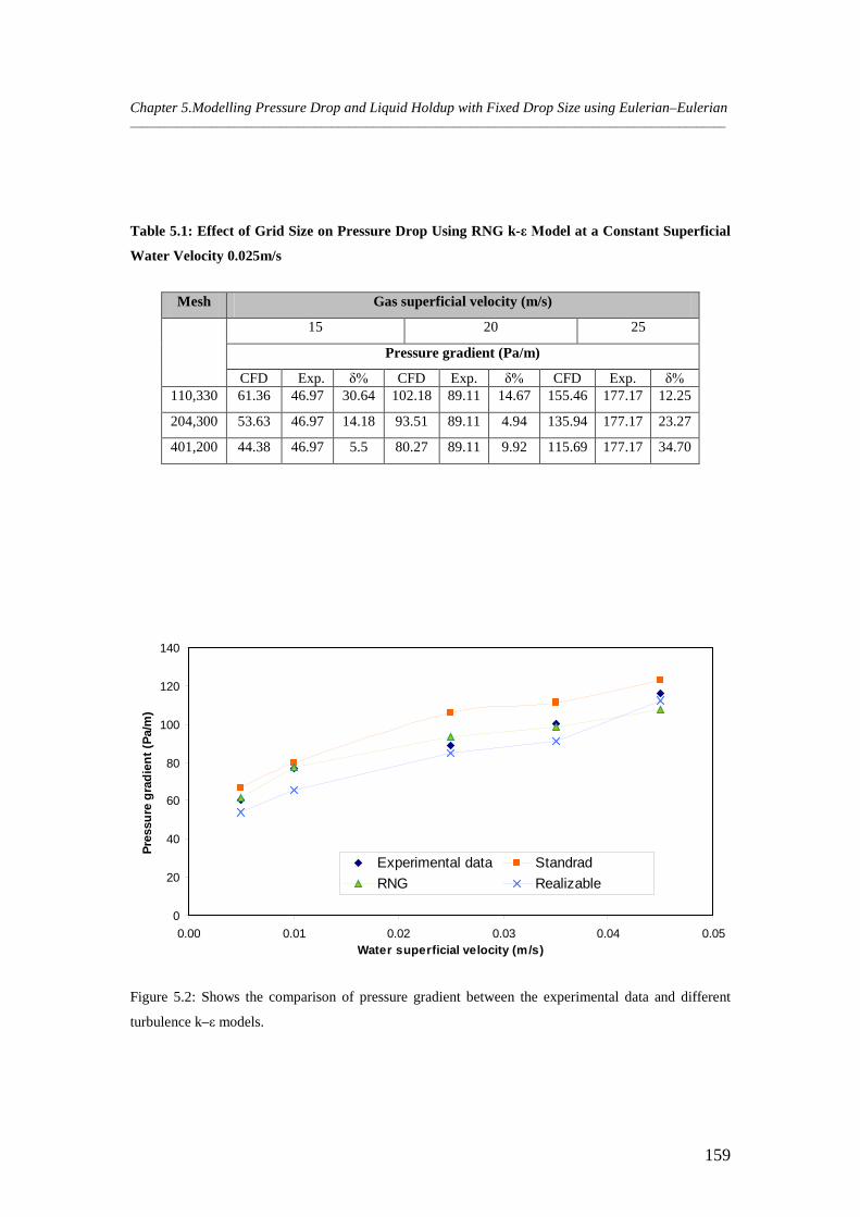
Chapter 5.Modelling Pressure Drop and Liquid Holdup with Fixed Drop Size using Eulerian–Eulerian _______________________________________________________________________________________________________
159
Table 5.1: Effect of Grid Size on Pressure Drop Using RNG k-ε Model at a Constant Superficial
Water Velocity 0.025m/s
Mesh Gas superficial velocity (m/s)
15 20 25
Pressure gradient (Pa/m)
CFD Exp. δ% CFD Exp. δ% CFD Exp. δ% 110,330 61.36 46.97 30.64 102.18 89.11 14.67 155.46 177.17 12.25
204,300 53.63 46.97 14.18 93.51 89.11 4.94 135.94 177.17 23.27
401,200 44.38 46.97 5.5 80.27 89.11 9.92 115.69 177.17 34.70
0
20
40
60
80
100
120
140
0.00 0.01 0.02 0.03 0.04 0.05Water superficial velocity (m/s)
Pre
ssu
re g
rad
ien
t (P
a/m
)
Experimental data Standrad
RNG Realizable
Figure 5.2: Shows the comparison of pressure gradient between the experimental data and different
turbulence k–ε models.
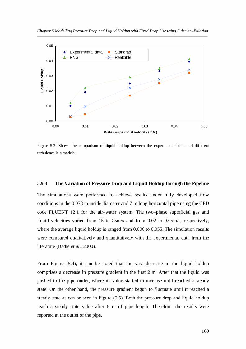
Chapter 5.Modelling Pressure Drop and Liquid Holdup with Fixed Drop Size using Eulerian–Eulerian _______________________________________________________________________________________________________
160
0.00
0.01
0.02
0.03
0.04
0.05
0.00 0.01 0.02 0.03 0.04 0.05
Water superficial velocity (m/s)
Liq
uid
Ho
ldu
p
Experimental data StandradRNG Realzible
Figure 5.3: Shows the comparison of liquid holdup between the experimental data and different
turbulence k–ε models.
5.9.3 The Variation of Pressure Drop and Liquid Holdup through the Pipeline
The simulations were performed to achieve results under fully developed flow
conditions in the 0.078 m inside diameter and 7 m long horizontal pipe using the CFD
code FLUENT 12.1 for the air–water system. The two–phase superficial gas and
liquid velocities varied from 15 to 25m/s and from 0.02 to 0.05m/s, respectively,
where the average liquid holdup is ranged from 0.006 to 0.055. The simulation results
were compared qualitatively and quantitatively with the experimental data from the
literature (Badie et al., 2000).
From Figure (5.4), it can be noted that the vast decrease in the liquid holdup
comprises a decrease in pressure gradient in the first 2 m. After that the liquid was
pushed to the pipe outlet, where its value started to increase until reached a steady
state. On the other hand, the pressure gradient begun to fluctuate until it reached a
steady state as can be seen in Figure (5.5). Both the pressure drop and liquid holdup
reach a steady state value after 6 m of pipe length. Therefore, the results were
reported at the outlet of the pipe.
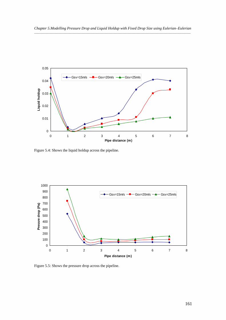
Chapter 5.Modelling Pressure Drop and Liquid Holdup with Fixed Drop Size using Eulerian–Eulerian _______________________________________________________________________________________________________
161
0
0.01
0.02
0.03
0.04
0.05
0 1 2 3 4 5 6 7 8Pipe distance (m)
Liq
uid
ho
ldu
p
Gsv=15m/s Gsv=20m/s Gsv=25m/s
Figure 5.4: Shows the liquid holdup across the pipeline.
0
100
200
300
400
500
600
700
800
900
1000
0 1 2 3 4 5 6 7 8
Pipe distance (m)
Pre
ssre
dro
p (
Pa)
Gsv=15m/s Gsv=20m/s Gsv=25m/s
Figure 5.5: Shows the pressure drop across the pipeline.
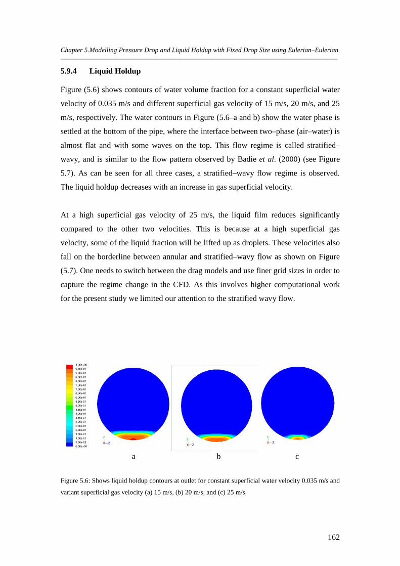
Chapter 5.Modelling Pressure Drop and Liquid Holdup with Fixed Drop Size using Eulerian–Eulerian _______________________________________________________________________________________________________
162
5.9.4 Liquid Holdup
Figure (5.6) shows contours of water volume fraction for a constant superficial water
velocity of 0.035 m/s and different superficial gas velocity of 15 m/s, 20 m/s, and 25
m/s, respectively. The water contours in Figure (5.6–a and b) show the water phase is
settled at the bottom of the pipe, where the interface between two–phase (air–water) is
almost flat and with some waves on the top. This flow regime is called stratified–
wavy, and is similar to the flow pattern observed by Badie et al. (2000) (see Figure
5.7). As can be seen for all three cases, a stratified–wavy flow regime is observed.
The liquid holdup decreases with an increase in gas superficial velocity.
At a high superficial gas velocity of 25 m/s, the liquid film reduces significantly
compared to the other two velocities. This is because at a high superficial gas
velocity, some of the liquid fraction will be lifted up as droplets. These velocities also
fall on the borderline between annular and stratified–wavy flow as shown on Figure
(5.7). One needs to switch between the drag models and use finer grid sizes in order to
capture the regime change in the CFD. As this involves higher computational work
for the present study we limited our attention to the stratified wavy flow.
Figure 5.6: Shows liquid holdup contours at outlet for constant superficial water velocity 0.035 m/s and
variant superficial gas velocity (a) 15 m/s, (b) 20 m/s, and (c) 25 m/s.
a b c
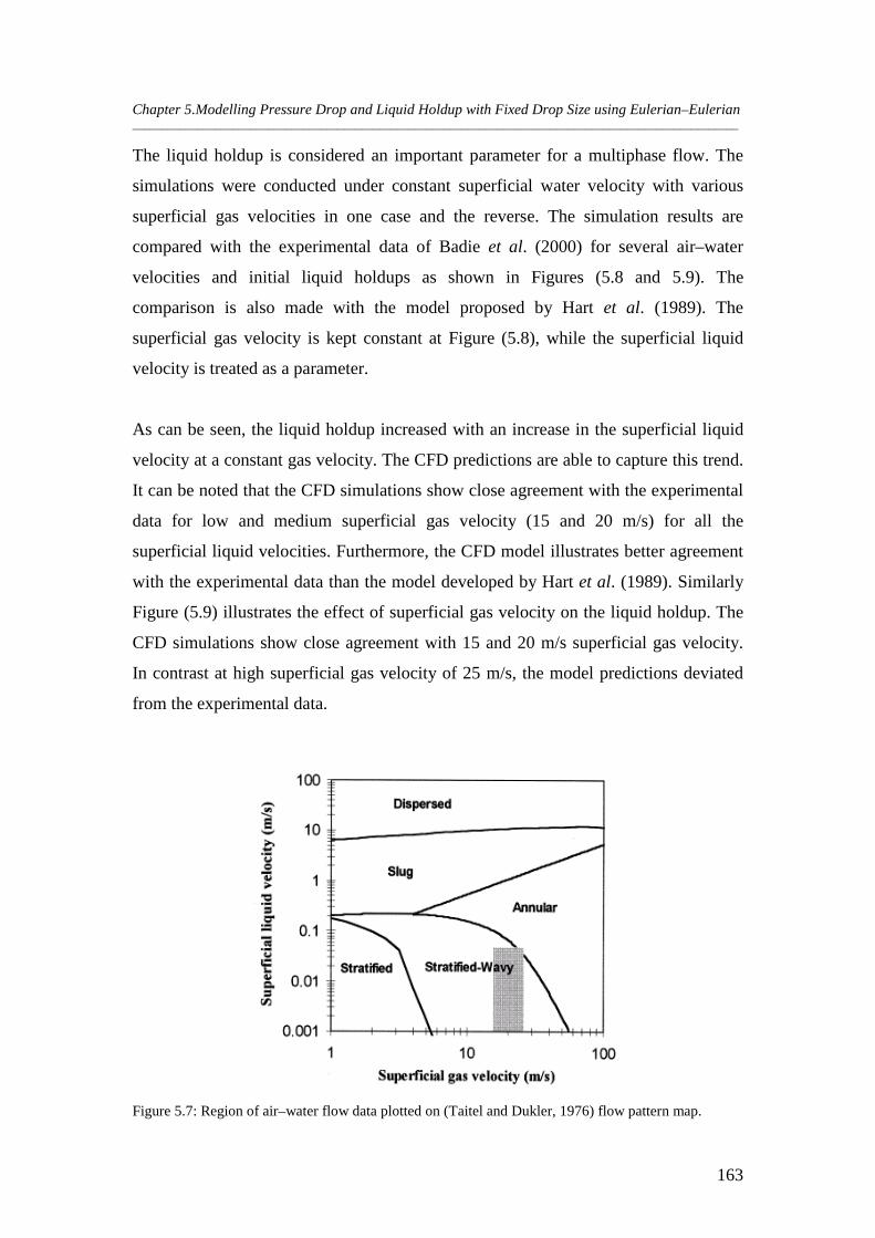
Chapter 5.Modelling Pressure Drop and Liquid Holdup with Fixed Drop Size using Eulerian–Eulerian _______________________________________________________________________________________________________
163
The liquid holdup is considered an important parameter for a multiphase flow. The
simulations were conducted under constant superficial water velocity with various
superficial gas velocities in one case and the reverse. The simulation results are
compared with the experimental data of Badie et al. (2000) for several air–water
velocities and initial liquid holdups as shown in Figures (5.8 and 5.9). The
comparison is also made with the model proposed by Hart et al. (1989). The
superficial gas velocity is kept constant at Figure (5.8), while the superficial liquid
velocity is treated as a parameter.
As can be seen, the liquid holdup increased with an increase in the superficial liquid
velocity at a constant gas velocity. The CFD predictions are able to capture this trend.
It can be noted that the CFD simulations show close agreement with the experimental
data for low and medium superficial gas velocity (15 and 20 m/s) for all the
superficial liquid velocities. Furthermore, the CFD model illustrates better agreement
with the experimental data than the model developed by Hart et al. (1989). Similarly
Figure (5.9) illustrates the effect of superficial gas velocity on the liquid holdup. The
CFD simulations show close agreement with 15 and 20 m/s superficial gas velocity.
In contrast at high superficial gas velocity of 25 m/s, the model predictions deviated
from the experimental data.
Figure 5.7: Region of air–water flow data plotted on (Taitel and Dukler, 1976) flow pattern map.
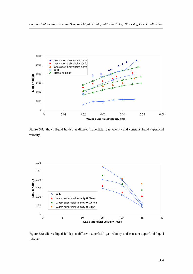
Chapter 5.Modelling Pressure Drop and Liquid Holdup with Fixed Drop Size using Eulerian–Eulerian _______________________________________________________________________________________________________
164
0
0.01
0.02
0.03
0.04
0.05
0.06
0 0.01 0.02 0.03 0.04 0.05 0.06
Water superficial velocity (m/s)
Liq
uid
ho
ldu
p
Gas superficial velocity 15m/sGas superficial velocity 20m/sGas superficial velocity 25m/sCFD Hart et al. Model
Figure 5.8: Shows liquid holdup at different superficial gas velocity and constant liquid superficial
velocity.
0
0.01
0.02
0.03
0.04
0.05
0.06
0 5 10 15 20 25 30
Gas superficial velocity (m/s)
Liq
uid
ho
ldu
p
CFD
w ater superficial velocity 0.02m/s
w ater superficial velocity 0.035m/s
w ater superficial velocity 0.05m/s
Figure 5.9: Shows liquid holdup at different superficial gas velocity and constant superficial liquid
velocity.
Chapter 5.Modelling Pressure Drop and Liquid Holdup with Fixed Drop Size using Eulerian–Eulerian _______________________________________________________________________________________________________
165
5.9.5 Pressure Gradient
In order to study the effect of a superficial velocity of gas and liquid on the pressure
gradient of two–phase flow in horizontal pipes, different simulation studies were
performed with several air and water superficial velocities ranging from 15 to 25m/s,
and 0.02 to 0.05m/s, respectively. The results were compared with experimental data
(Badie et al., 2000) and also with the models developed by Hart et al., (1989) and
Chen et al. (1997). Figure (5.10) shows the relationship between the superficial water
velocity and pressure gradient in which the superficial gas velocity is kept constant.
It can be noted that the pressure gradient increases with the superficial water velocity
as shown on Figure (5.10–a and b). The rate of increase can be seen clearly as the
superficial gas velocity also increased. At low superficial gas velocity the pressure
gradient changes cannot be distinguished with variant superficial water velocity, and
is represented as a straight line.
The pressure gradient results at low superficial gas velocity are well predicted by
CFD simulations with respect to experimental data. In contrast the Hart et al. (1989)
and Chen et al. (1997) developed models over predicted the pressure gradient at low
and medium superficial gas velocities of 15 and 20 m/s respectively. However at high
superficial gas velocity, the Hart and Chen models predicted pressure gradient quite
well with respect to the Badie experimental data, especially at low superficial water
velocity according to the Hart model, and at medium superficial water velocity
according to the Chen model, where the CFD result under predicted.
Figure (5.11) demonstrates the effect of superficial gas velocity on the pressure
gradient at a stable superficial water velocity. It can be observed that an increase in
the water superficial velocity at a constant gas superficial velocity leads to a
substantial increase in the pressure gradient. In addition, it shows a close agreement
with low and medium gas superficial velocities of 15 and 20 m/s respectively, and
deviated at high gas superficial velocity (25 m/s). This is due to the fact that when the
gas flow rate is increased, a greater friction of pipe wall is covered by a rough
Chapter 5.Modelling Pressure Drop and Liquid Holdup with Fixed Drop Size using Eulerian–Eulerian _______________________________________________________________________________________________________
166
interface formed between the liquid and gas, which leads to an increased friction
factor and pressure gradient.
The validation of the model used in this study is achieved by comparison with
experimental data. The results were in close agreement in particular at a superficial
gas velocity lower than 25 m/s. Therefore, the model can be used for studying the
effect of different parameters on the pressure drop and liquid holdup in a horizontal
pipeline. In order to study these parameters, such as mass flux and initial liquid
holdup, on the pressure drop and liquid holdup simulations were performed for a
series of liquid holdup at a constant gas and liquid superficial velocity.
0
50
100
150
200
250
0 0.01 0.02 0.03 0.04 0.05 0.06
Water superficial velocity (m/s)
Pre
ss
ure
gra
die
nt
(Pa
/m)
Gas superficial velocity 15m/sGas superficial velocity 20m/sGas superficial velocity 25m/sCFDHart et al. Model
(a)
Chapter 5.Modelling Pressure Drop and Liquid Holdup with Fixed Drop Size using Eulerian–Eulerian _______________________________________________________________________________________________________
167
0
50
100
150
200
250
0 0.01 0.02 0.03 0.04 0.05 0.06
Water superficial velocity (m/s)
Pre
ss
ure
gra
die
nt
(Pa
/m)
Gas superficial velocity 15m/sGas superficial velocity 20m/sGas superficial velocity 25m/sCFDChen et al. Model
(b)
Figure 5.10: Shows CFD comparison of pressure gradient with an experimental data and (a) the Hart et
al. model and (b) the Chen et al. model.
0
50
100
150
200
250
0 5 10 15 20 25 30
Gas superficial velocity (m/s)
Pre
ssu
re g
rad
ien
t (P
a/m
)
w ater superficial velocity 0.02m/s
w ater superficial velocity 0.035m/s
w ater superficial velocity 0.05m/s
CFD
Figure 5.11: Shows CFD comparison of pressure gradient with an experimental data.
Chapter 5.Modelling Pressure Drop and Liquid Holdup with Fixed Drop Size using Eulerian–Eulerian _______________________________________________________________________________________________________
168
5.10 Effect of Different Parameters on Pressure Drop and Liquid Holdup
5.10.1 Effect of Droplet Size
This section has investigated the effect of droplet diameter on the pressure gradient
and liquid holdup at a high gas superficial velocity of 25 m/s. The previous
simulations were performed under constant droplet diameter (100 μm), where the
result deviated from the experimental data. Moreover, as we know that the droplet
sizes are not uniform in reality, it varies (e.g. from 10–1000 μm). The droplet size is
examined to capture the effect on the two–phase pressure drop and liquid holdup
parameters. The simulation was performed under a fixed droplet diameter of 300 μm.
Figure (5.12) represents the pressure gradient versus superficial water velocity at a
constant superficial gas velocity of 25 m/s. The CFD prediction result of pressure
gradient at a drop size of 300 μm is found to have closely followed the experimental
data as shown in Figure (5.12). It can also be observed that the CFD simulations data
confirm close agreement with the experimental data at a constant high gas superficial
velocity of 25 m/s with entire range of liquid (water) superficial velocities. In
addition, the CFD model confirms agreement with the experimental data, compared to
the model developed by Hart et al. (1989). On the other hand, Figure (5.13)
demonstrates the effect of water superficial velocity on the liquid holdup at a constant
gas superficial velocity of 25 m/s.
The CFD simulation results of a 300 μm drop size also show closer agreement with
the experimental data compared with the previous case study of 100 μm drop size. It
can also be observed clearly in Figure (5.14–b), in which the interface between the
two–phase is more obvious in comparison with the first simulation with 100 μm, as
shown in Figure (5.14–a), and represents the stratified flow. Additionally, at a 300 μm
droplet diameter, the model predictions of liquid holdup are predicted well at low
water superficial velocities between 0.02–0.025 m/s. At medium and high water
superficial velocities above 0.03 m/s, the CFD predictions of liquid holdup data are
over predicted compared with the model by Hart et al. (1989).
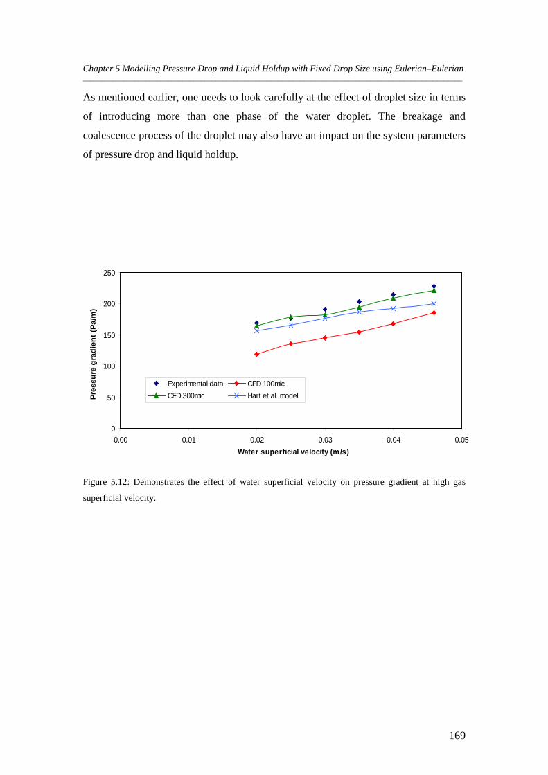
Chapter 5.Modelling Pressure Drop and Liquid Holdup with Fixed Drop Size using Eulerian–Eulerian _______________________________________________________________________________________________________
169
As mentioned earlier, one needs to look carefully at the effect of droplet size in terms
of introducing more than one phase of the water droplet. The breakage and
coalescence process of the droplet may also have an impact on the system parameters
of pressure drop and liquid holdup.
0
50
100
150
200
250
0.00 0.01 0.02 0.03 0.04 0.05
Water superficial velocity (m/s)
Pre
ssu
re g
rad
ien
t (P
a/m
)
Experimental data CFD 100mic
CFD 300mic Hart et al. model
Figure 5.12: Demonstrates the effect of water superficial velocity on pressure gradient at high gas
superficial velocity.
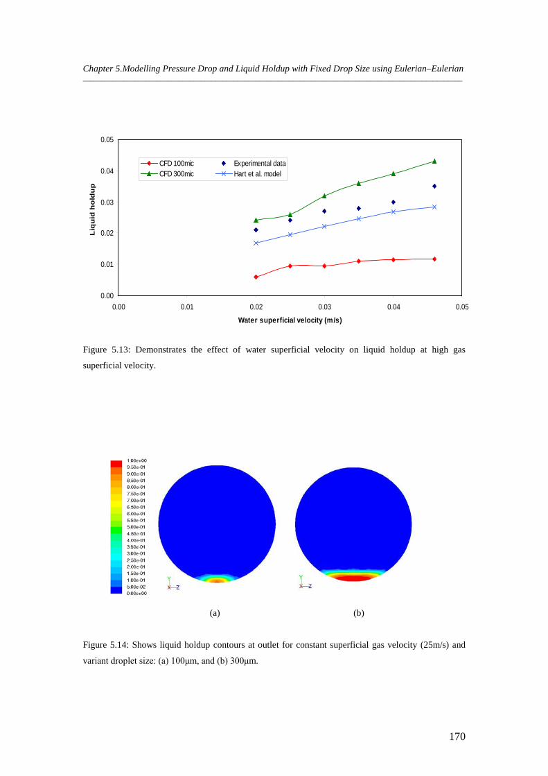
Chapter 5.Modelling Pressure Drop and Liquid Holdup with Fixed Drop Size using Eulerian–Eulerian _______________________________________________________________________________________________________
170
0.00
0.01
0.02
0.03
0.04
0.05
0.00 0.01 0.02 0.03 0.04 0.05
Water superficial velocity (m/s)
Liq
uid
ho
ldu
p
CFD 100mic Experimental data CFD 300mic Hart et al. model
Figure 5.13: Demonstrates the effect of water superficial velocity on liquid holdup at high gas
superficial velocity.
(a) (b)
Figure 5.14: Shows liquid holdup contours at outlet for constant superficial gas velocity (25m/s) and
variant droplet size: (a) 100μm, and (b) 300μm.
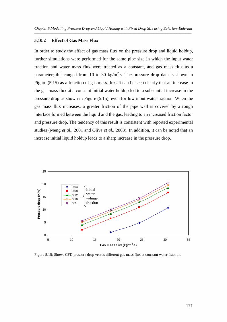
Chapter 5.Modelling Pressure Drop and Liquid Holdup with Fixed Drop Size using Eulerian–Eulerian _______________________________________________________________________________________________________
171
5.10.2 Effect of Gas Mass Flux
In order to study the effect of gas mass flux on the pressure drop and liquid holdup,
further simulations were performed for the same pipe size in which the input water
fraction and water mass flux were treated as a constant, and gas mass flux as a
parameter; this ranged from 10 to 30 kg/m2.s. The pressure drop data is shown in
Figure (5.15) as a function of gas mass flux. It can be seen clearly that an increase in
the gas mass flux at a constant initial water holdup led to a substantial increase in the
pressure drop as shown in Figure (5.15), even for low input water fraction. When the
gas mass flux increases, a greater friction of the pipe wall is covered by a rough
interface formed between the liquid and the gas, leading to an increased friction factor
and pressure drop. The tendency of this result is consistent with reported experimental
studies (Meng et al., 2001 and Olive et al., 2003). In addition, it can be noted that an
increase initial liquid holdup leads to a sharp increase in the pressure drop.
0
5
10
15
20
25
5 10 15 20 25 30 35
Gas mass flux (kg/m2.s)
Pre
ssu
re d
rop
(K
Pa)
0.040.080.120.160.2
Figure 5.15: Shows CFD pressure drop versus different gas mass flux at constant water fraction.
Initial water volume fraction
Chapter 5.Modelling Pressure Drop and Liquid Holdup with Fixed Drop Size using Eulerian–Eulerian _______________________________________________________________________________________________________
172
On the other hand, the simulation results obtained of liquid holdup for air–water flow
were plotted versus gas mass flux with different initial water fractions which varied
from 0.04 to 0.2, and are treated as a factor in Figure (5.16). It can be observed that
the liquid holdup decreases with increasing gas mass flux at different initial water
holdup. This is due to the increase of the interfacial shear stress at larger velocity
differences between the gas and liquid fluid, where this result of decreasing liquid
holdup with increasing gas mass flux was expected. This observation was similar to
that reported in experimental data of gas–liquid flow with low liquid loading in
horizontal pipes by Meng et al. (2001).
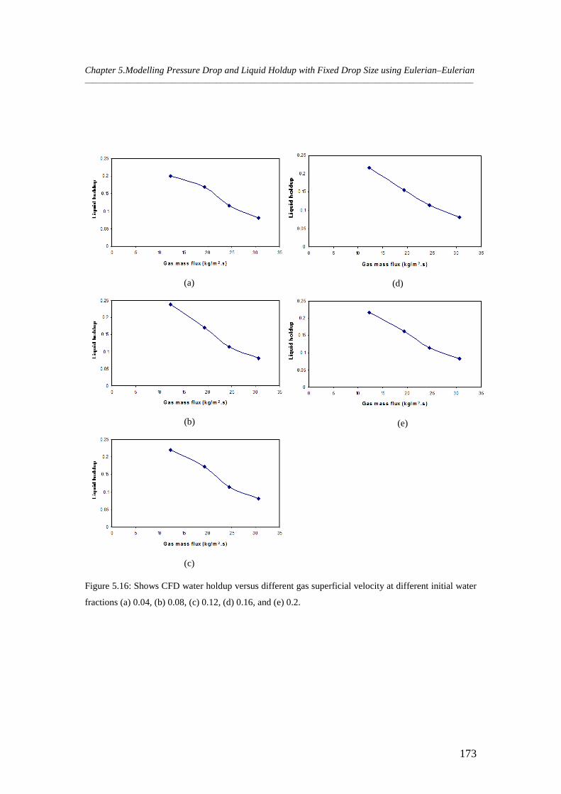
Chapter 5.Modelling Pressure Drop and Liquid Holdup with Fixed Drop Size using Eulerian–Eulerian _______________________________________________________________________________________________________
173
(a)
(b)
(c)
(d)
(e)
Figure 5.16: Shows CFD water holdup versus different gas superficial velocity at different initial water
fractions (a) 0.04, (b) 0.08, (c) 0.12, (d) 0.16, and (e) 0.2.
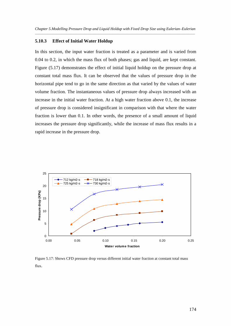
Chapter 5.Modelling Pressure Drop and Liquid Holdup with Fixed Drop Size using Eulerian–Eulerian _______________________________________________________________________________________________________
174
5.10.3 Effect of Initial Water Holdup
In this section, the input water fraction is treated as a parameter and is varied from
0.04 to 0.2, in which the mass flux of both phases; gas and liquid, are kept constant.
Figure (5.17) demonstrates the effect of initial liquid holdup on the pressure drop at
constant total mass flux. It can be observed that the values of pressure drop in the
horizontal pipe tend to go in the same direction as that varied by the values of water
volume fraction. The instantaneous values of pressure drop always increased with an
increase in the initial water fraction. At a high water fraction above 0.1, the increase
of pressure drop is considered insignificant in comparison with that where the water
fraction is lower than 0.1. In other words, the presence of a small amount of liquid
increases the pressure drop significantly, while the increase of mass flux results in a
rapid increase in the pressure drop.
0
5
10
15
20
25
0.00 0.05 0.10 0.15 0.20 0.25
Water volume fraction
Pre
ssu
re d
rop
(K
Pa)
712 kg/m2-s 718 kg/m2-s725 kg/m2-s 730 kg/m2-s
Figure 5.17: Shows CFD pressure drop versus different initial water fraction at constant total mass
flux.
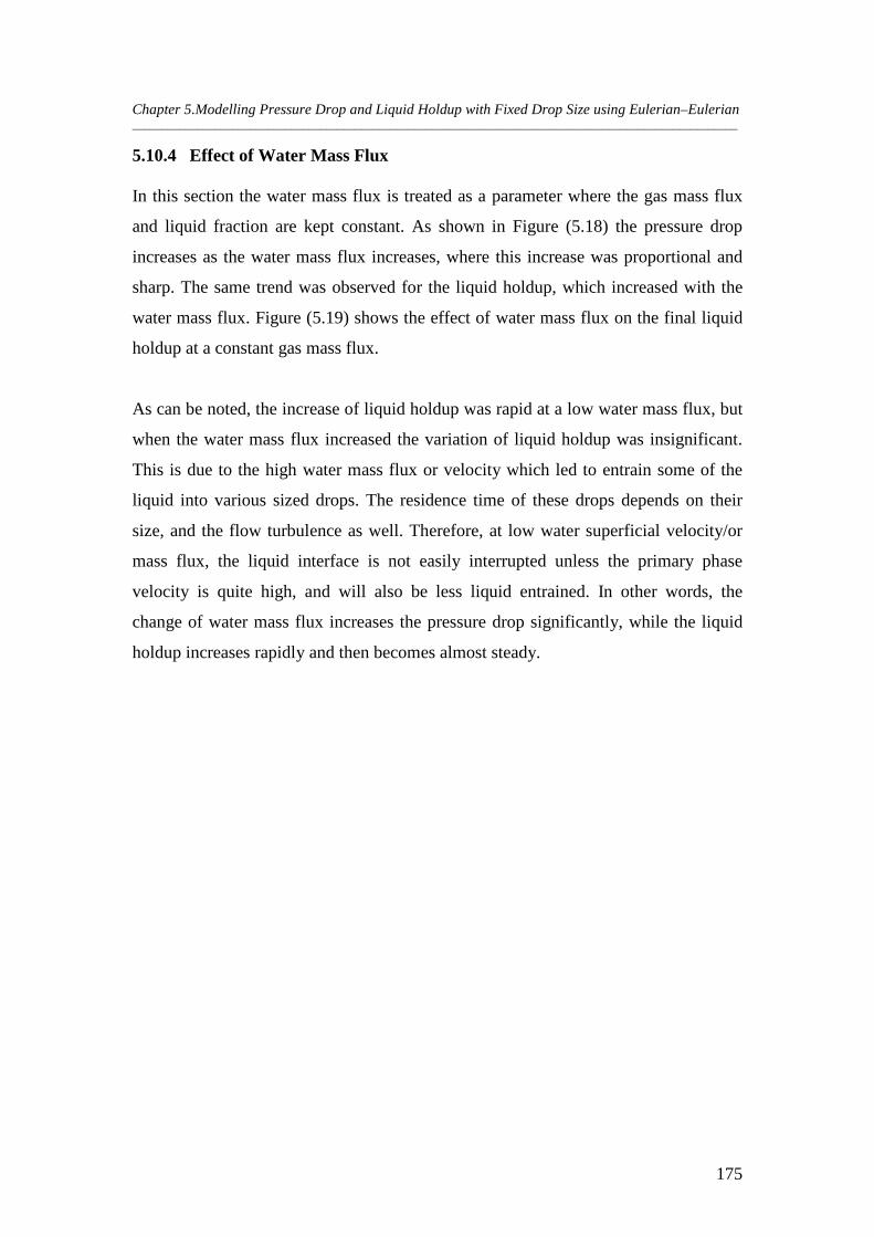
Chapter 5.Modelling Pressure Drop and Liquid Holdup with Fixed Drop Size using Eulerian–Eulerian _______________________________________________________________________________________________________
175
5.10.4 Effect of Water Mass Flux
In this section the water mass flux is treated as a parameter where the gas mass flux
and liquid fraction are kept constant. As shown in Figure (5.18) the pressure drop
increases as the water mass flux increases, where this increase was proportional and
sharp. The same trend was observed for the liquid holdup, which increased with the
water mass flux. Figure (5.19) shows the effect of water mass flux on the final liquid
holdup at a constant gas mass flux.
As can be noted, the increase of liquid holdup was rapid at a low water mass flux, but
when the water mass flux increased the variation of liquid holdup was insignificant.
This is due to the high water mass flux or velocity which led to entrain some of the
liquid into various sized drops. The residence time of these drops depends on their
size, and the flow turbulence as well. Therefore, at low water superficial velocity/or
mass flux, the liquid interface is not easily interrupted unless the primary phase
velocity is quite high, and will also be less liquid entrained. In other words, the
change of water mass flux increases the pressure drop significantly, while the liquid
holdup increases rapidly and then becomes almost steady.
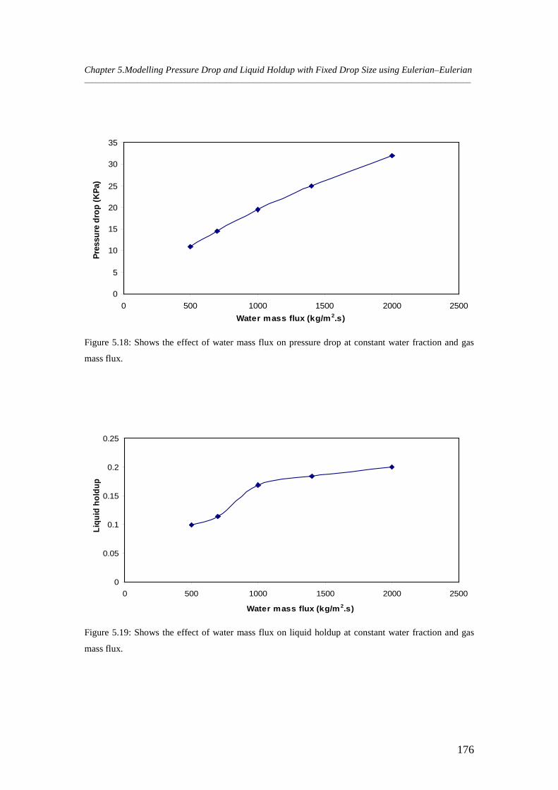
Chapter 5.Modelling Pressure Drop and Liquid Holdup with Fixed Drop Size using Eulerian–Eulerian _______________________________________________________________________________________________________
176
0
5
10
15
20
25
30
35
0 500 1000 1500 2000 2500
Water mass flux (kg/m2.s)
Pre
ssu
re d
rop
(K
Pa)
Figure 5.18: Shows the effect of water mass flux on pressure drop at constant water fraction and gas
mass flux.
0
0.05
0.1
0.15
0.2
0.25
0 500 1000 1500 2000 2500
Water mass flux (kg/m2.s)
Liq
uid
ho
ldu
p
Figure 5.19: Shows the effect of water mass flux on liquid holdup at constant water fraction and gas
mass flux.
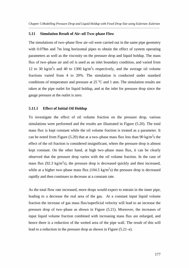
Chapter 5.Modelling Pressure Drop and Liquid Holdup with Fixed Drop Size using Eulerian–Eulerian _______________________________________________________________________________________________________
177
5.11 Simulation Result of Air–oil Two–phase Flow
The simulations of two–phase flow air–oil were carried out in the same pipe geometry
with 0.078m and 7m long horizontal pipes to obtain the effect of system operating
parameters as well as the viscosity on the pressure drop and liquid holdup. The mass
flux of two–phase air and oil is used as an inlet boundary condition, and varied from
12 to 30 kg/m2s and 40 to 1300 kg/m2s respectively, and the average oil volume
fractions varied from 4 to 20%. The simulation is conducted under standard
conditions of temperature and pressure at 25 oC and 1 atm. The simulation results are
taken at the pipe outlet for liquid holdup, and at the inlet for pressure drop since the
gauge pressure at the outlet is zero.
5.11.1 Effect of Initial Oil Holdup
To investigate the effect of oil volume fraction on the pressure drop, various
simulations were performed and the results are illustrated in Figure (5.20). The total
mass flux is kept constant while the oil volume fraction is treated as a parameter. It
can be noted from Figure (5.20) that at a two–phase mass flux less than 90 kg/m2s the
effect of the oil fraction is considered insignificant, where the pressure drop is almost
kept constant. On the other hand, at high two–phase mass flux, it can be clearly
observed that the pressure drop varies with the oil volume fraction. In the case of
mass flux (92.3 kg/m2s), the pressure drop is decreased quickly and then increased,
while at a higher two–phase mass flux (104.5 kg/m2s) the pressure drop is decreased
rapidly and then continues to decrease at a constant rate.
As the total flow rate increased, more drops would expect to entrain in the inner pipe,
leading to a decrease the real area of the gas. At a constant input liquid volume
fraction the increase of gas mass flux/superficial velocity will lead to an increase the
pressure drop of two–phase as shown in Figure (5.21). Moreover, the increases of
input liquid volume fraction combined with increasing mass flux are enlarged, and
hence there is a reduction of the wetted area of the pipe wall. The result of this will
lead to a reduction in the pressure drop as shown in Figure (5.21–e).
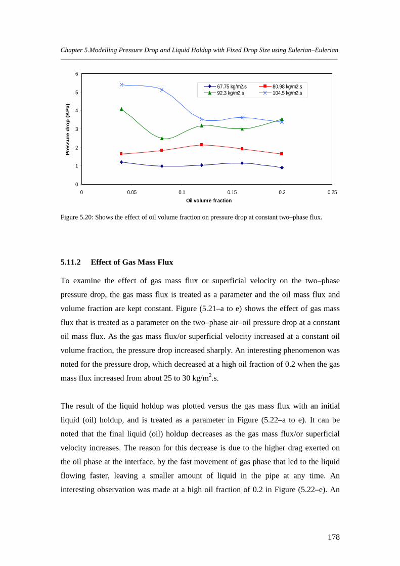
Chapter 5.Modelling Pressure Drop and Liquid Holdup with Fixed Drop Size using Eulerian–Eulerian _______________________________________________________________________________________________________
178
0
1
2
3
4
5
6
0 0.05 0.1 0.15 0.2 0.25
Oil volume fraction
Pre
ssu
re d
rop
(K
Pa)
67.75 kg/m2.s 80.98 kg/m2.s92.3 kg/m2.s 104.5 kg/m2.s
Figure 5.20: Shows the effect of oil volume fraction on pressure drop at constant two–phase flux.
5.11.2 Effect of Gas Mass Flux
To examine the effect of gas mass flux or superficial velocity on the two–phase
pressure drop, the gas mass flux is treated as a parameter and the oil mass flux and
volume fraction are kept constant. Figure (5.21–a to e) shows the effect of gas mass
flux that is treated as a parameter on the two–phase air–oil pressure drop at a constant
oil mass flux. As the gas mass flux/or superficial velocity increased at a constant oil
volume fraction, the pressure drop increased sharply. An interesting phenomenon was
noted for the pressure drop, which decreased at a high oil fraction of 0.2 when the gas
mass flux increased from about 25 to 30 kg/m2.s.
The result of the liquid holdup was plotted versus the gas mass flux with an initial
liquid (oil) holdup, and is treated as a parameter in Figure (5.22–a to e). It can be
noted that the final liquid (oil) holdup decreases as the gas mass flux/or superficial
velocity increases. The reason for this decrease is due to the higher drag exerted on
the oil phase at the interface, by the fast movement of gas phase that led to the liquid
flowing faster, leaving a smaller amount of liquid in the pipe at any time. An
interesting observation was made at a high oil fraction of 0.2 in Figure (5.22–e). An
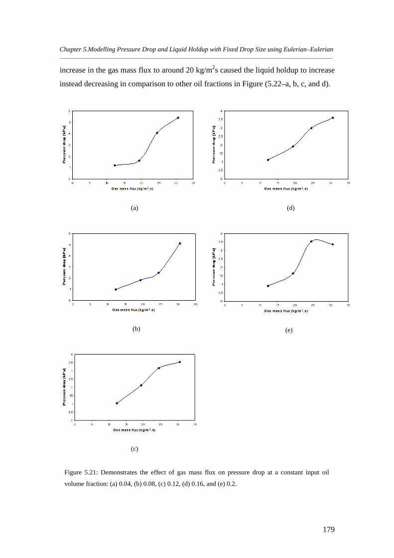
Chapter 5.Modelling Pressure Drop and Liquid Holdup with Fixed Drop Size using Eulerian–Eulerian _______________________________________________________________________________________________________
179
increase in the gas mass flux to around 20 kg/m2s caused the liquid holdup to increase
instead decreasing in comparison to other oil fractions in Figure (5.22–a, b, c, and d).
(a)
(b)
(c)
(d)
(e)
Figure 5.21: Demonstrates the effect of gas mass flux on pressure drop at a constant input oil
volume fraction: (a) 0.04, (b) 0.08, (c) 0.12, (d) 0.16, and (e) 0.2.
Chapter 5.Modelling Pressure Drop and Liquid Holdup with Fixed Drop Size using Eulerian–Eulerian _______________________________________________________________________________________________________
180
(a)
(b)
(c)
(d)
(e)
Figure 5.22: Demonstrates the effect of gas mass flux on liquid holdup at a constant input oil
volume fraction: (a) 0.04, (b) 0.08, (c) 0.12, (d) 0.16, and (e) 0.2.
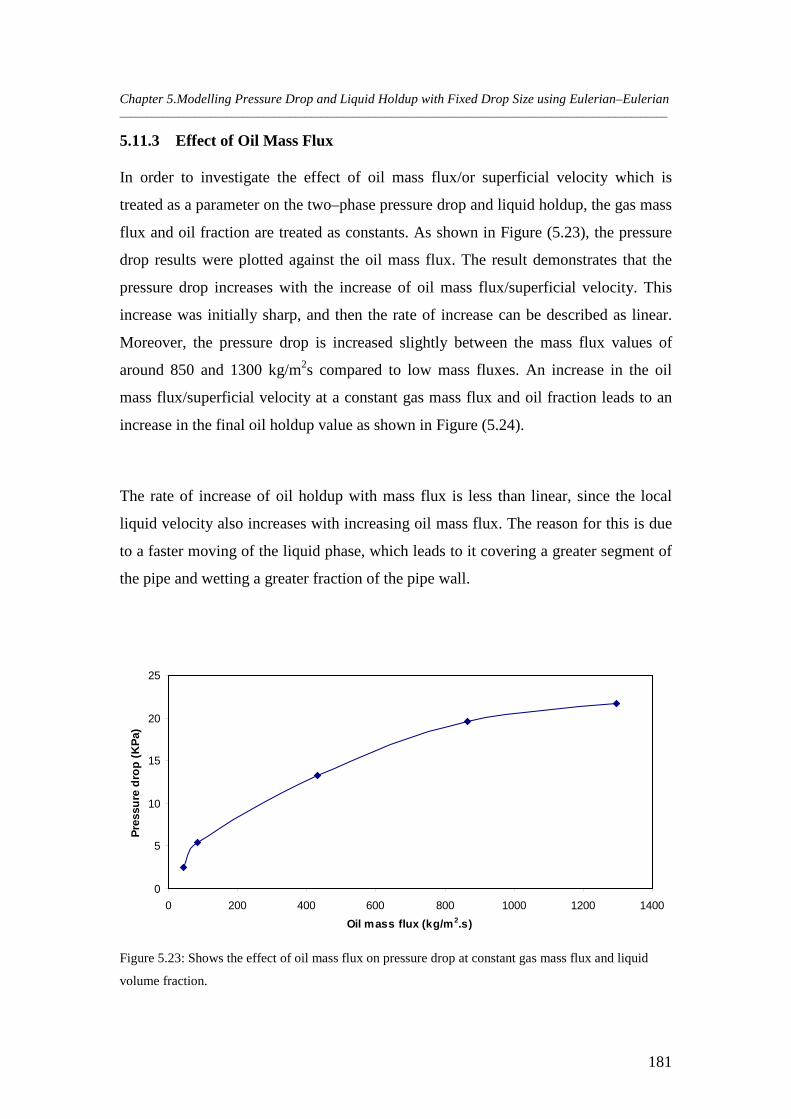
Chapter 5.Modelling Pressure Drop and Liquid Holdup with Fixed Drop Size using Eulerian–Eulerian _______________________________________________________________________________________________________
181
5.11.3 Effect of Oil Mass Flux
In order to investigate the effect of oil mass flux/or superficial velocity which is
treated as a parameter on the two–phase pressure drop and liquid holdup, the gas mass
flux and oil fraction are treated as constants. As shown in Figure (5.23), the pressure
drop results were plotted against the oil mass flux. The result demonstrates that the
pressure drop increases with the increase of oil mass flux/superficial velocity. This
increase was initially sharp, and then the rate of increase can be described as linear.
Moreover, the pressure drop is increased slightly between the mass flux values of
around 850 and 1300 kg/m2s compared to low mass fluxes. An increase in the oil
mass flux/superficial velocity at a constant gas mass flux and oil fraction leads to an
increase in the final oil holdup value as shown in Figure (5.24).
The rate of increase of oil holdup with mass flux is less than linear, since the local
liquid velocity also increases with increasing oil mass flux. The reason for this is due
to a faster moving of the liquid phase, which leads to it covering a greater segment of
the pipe and wetting a greater fraction of the pipe wall.
0
5
10
15
20
25
0 200 400 600 800 1000 1200 1400
Oil mass flux (kg/m2.s)
Pre
ssu
re d
rop
(K
Pa)
Figure 5.23: Shows the effect of oil mass flux on pressure drop at constant gas mass flux and liquid
volume fraction.
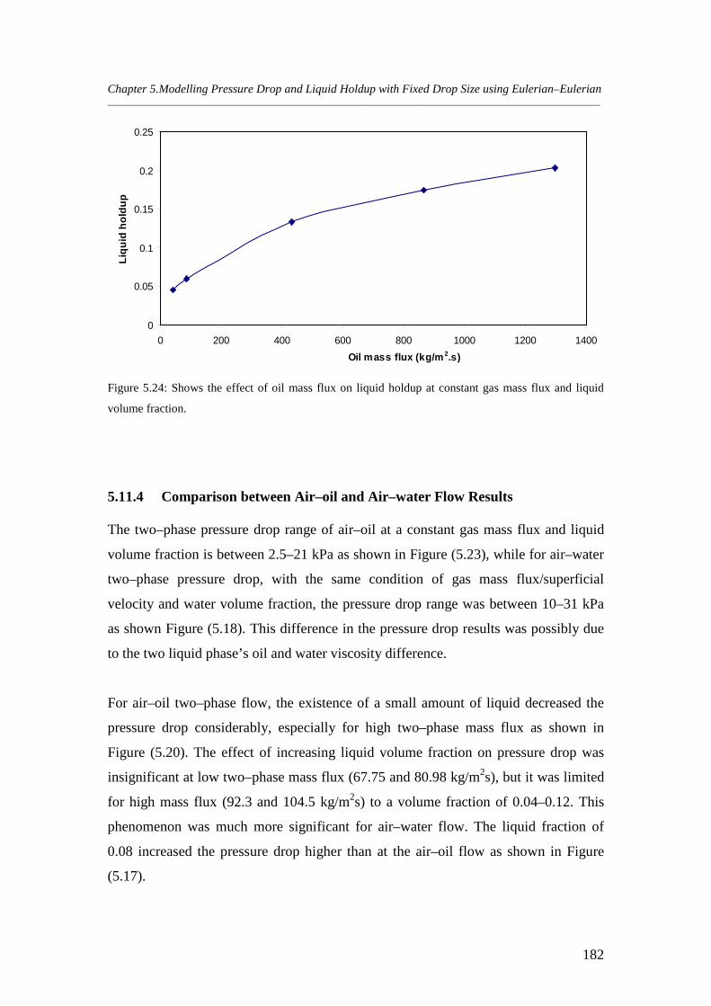
Chapter 5.Modelling Pressure Drop and Liquid Holdup with Fixed Drop Size using Eulerian–Eulerian _______________________________________________________________________________________________________
182
0
0.05
0.1
0.15
0.2
0.25
0 200 400 600 800 1000 1200 1400
Oil mass flux (kg/m2.s)
Liq
uid
ho
ldu
p
Figure 5.24: Shows the effect of oil mass flux on liquid holdup at constant gas mass flux and liquid
volume fraction.
5.11.4 Comparison between Air–oil and Air–water Flow Results
The two–phase pressure drop range of air–oil at a constant gas mass flux and liquid
volume fraction is between 2.5–21 kPa as shown in Figure (5.23), while for air–water
two–phase pressure drop, with the same condition of gas mass flux/superficial
velocity and water volume fraction, the pressure drop range was between 10–31 kPa
as shown Figure (5.18). This difference in the pressure drop results was possibly due
to the two liquid phase’s oil and water viscosity difference.
For air–oil two–phase flow, the existence of a small amount of liquid decreased the
pressure drop considerably, especially for high two–phase mass flux as shown in
Figure (5.20). The effect of increasing liquid volume fraction on pressure drop was
insignificant at low two–phase mass flux (67.75 and 80.98 kg/m2s), but it was limited
for high mass flux (92.3 and 104.5 kg/m2s) to a volume fraction of 0.04–0.12. This
phenomenon was much more significant for air–water flow. The liquid fraction of
0.08 increased the pressure drop higher than at the air–oil flow as shown in Figure
(5.17).
Chapter 5.Modelling Pressure Drop and Liquid Holdup with Fixed Drop Size using Eulerian–Eulerian _______________________________________________________________________________________________________
183
For air–oil two–phase flow, it was observed that the pressure drop decreased when the
liquid volume fraction increased from 0.04–0.12 at a high superficial gas velocity of
20–25 m/s. This phenomenon was not seen with air–water two–phase flow where the
two–phase pressure drop was noted to increase until the increase in the liquid fraction
was less significant on the pressure drop change.
The result obtained for the liquid holdup for air–water was greater than for the air–oil
two–phase flow. In the case of air–water two–phase flow, the range of liquid holdup
was 0.2–0.24 for a gas mass flux of 12.25 kg/m2s, which corresponds to 10 m/s and
0.08–0.084 for 30.63 kg/m2s (corresponding to 25 m/s). On the other hand, the air–oil
liquid holdup range was 0.1–0.12 for a gas mass flux of 12.25 kg/m2s and 0.016–
0.027 for a gas mass flux of 30.63 kg/m2s. Moreover, the phenomenon of decreasing
the liquid holdup with the increase in the initial liquid volume fraction was observed
for varying gas mass flux values/superficial velocities in both cases of two–phase
flow. However as the liquid holdup at air–water is greater than for air–oil, this could
be that the flow pattern in each of these two–phase flows is different, annular flow for
air–water and stratified wavy flow for air–oil. This would be expected due to the
viscosity difference.
5.12 Comparison of CFD Result with An empirical Correlation
As mentioned in Chapter 2, different empirical correlations have been developed
based on experimental data for calculating the pressure drop and liquid holdup. One
of these correlations is the Beggs and Brill (1973) (labelled “B–B”) correlation
analysis. This is based on experimental data for air–water flow in small tubes with
various inclination angles and has been widely used to describe the pressure drop in a
horizontal pipe of two–phase flow that may be encountered in oil and gas
transportation, although numerous empirical or semi–empirical models are available
in the literature.
The Beggs and Brill correlation can be used to find the friction pressure loss and the
hydrostatic pressure difference, which is not included here since the pipeline used is
horizontal. The two–phase flow pattern defined as Segregated, Intermittent or
Chapter 5.Modelling Pressure Drop and Liquid Holdup with Fixed Drop Size using Eulerian–Eulerian _______________________________________________________________________________________________________
184
Distributed is obtained based on the Beggs and Brill parameters. Then the liquid
holdup and in-situ density of two–phase mixture is computed based on the flow
regime. The gas–liquid two–phase flow friction factor is obtained based on the input
ratio of two–phase and the Fanning friction factor. Based on this the friction pressure
drop can be estimated using the input mixture properties of two phases.
5.12.1 Identified Flow Pattern
To identify the flow pattern, transition lines are obtained as follows:
738.64
4516.13
4684.252
302.01
5.0
1.0
1052.92
316
−
−
−−
=
=
×=
=
λ
λ
λ
λ
LLLL
Where L1, L2, L3, and L4 are Beggs and Brill parameters, and λ is the initial liquid
holdup that is calculated using this equation:
m
l
uu
=λ (5.15)
Where ul is the liquid velocity and um is the mixture velocity. The flow pattern is
determined either from the existence of a flow pattern map or based on the following
conditions of the correlation as:
gDuFr m
m
2
= (5.16)
To find out one of the flow patterns (Segregated, Intermittent or Distributed), the
following conditions are applied:
• The flow is described as Segregated if
λ < 0.01 and Frm < L1 or λ > 0.01 and Frm < L2
(5.14)
Chapter 5.Modelling Pressure Drop and Liquid Holdup with Fixed Drop Size using Eulerian–Eulerian _______________________________________________________________________________________________________
185
• The flow is described as Transition if
λ ≥ 0.01 and L2 < Frm ≤ L3
• The flow is described as Intermittent if
0.01 ≤ λ < 0.4 and L3 < Frm ≤ L1 or λ ≥ 0.4 and L3 < Frm ≤ L4
• The flow is described as Distributed if
λ < 0.4 and Frm ≥ L1 or λ ≥ 0.4 and Frm > L4
5.12.2 Two–phase Pressure Drop
In order to calculate the pressure drop due to friction, the empirical parameter “S” is
obtained using one of the following formulas based on the “y” value.
if 1 < y < 1.2, then
)2.12.2ln( −= yS (5.17)
Otherwise
42 01853.08725.0182.30523.0 yyyyS
+−+−= (5.18)
where y can be defined as,
αλln=y and C
m
B
FrAλα = (5.19)
where A, B and C are constants and depend on the flow regime
Chapter 5.Modelling Pressure Drop and Liquid Holdup with Fixed Drop Size using Eulerian–Eulerian _______________________________________________________________________________________________________
186
The two–phase friction factor is obtained from equation (5.19) based on no–slip
friction factor, which is based on no–slip Reynolds number that is calculated as
follows:
mix
mixmixns
DVµ
ρ=Re (5.20)
The Blasius equation for the Fanning friction factor can be written as:
nns
nsxf
Re= (5.21)
where x = 16 and n = 1.0 for laminar flow (Re < 2000), while x = 0.079 and n = 0.25
for turbulent flow (Re > 2000). The two-phase friction factor is calculated as:
s
nseff = (5.22)
The two –phase pressure drop due to friction can be expressed as:
DVfP mixmix
22 ρ=∆ (5.23)
5.12.3 Liquid Holdup Correlation
The liquid holdup correlation used in this investigation, is the Mukherjee and Brill
(1985) (Labelled “M–B”) correlation developed for different pipe inclination angles.
In this research we will focus on the horizontal segment and exclude the uphill section
of the correlation. The general liquid holdup correlation is presented in the equation
(5.24) below.
( )
+++=
6
52
42
321 sinsinexp CLv
Cgv
LL NN
NCCCCH θθ (5.24)
Chapter 5.Modelling Pressure Drop and Liquid Holdup with Fixed Drop Size using Eulerian–Eulerian _______________________________________________________________________________________________________
187
The second and third terms in the equation are equal to zero because the pipe is
horizontal. C1, C2, C3, C4, C5, and C6 are regression coefficients depending on flow
direction uphill, downhill and horizontal. Ngv, NLv, and NL are the gas velocity number,
liquid velocity number and liquid viscosity number, respectively. They can be
obtained as follows:
25.0
=
l
lsggv g
vNσρ (5.25)
25.0
=
l
lslLv g
vNσρ (5.26)
25.0
3
=
llLL
gNσρ
µ (5.27)
5.12.4 Results and Discussion The Beggs and Brill correlation has been tested at two different initial liquid (water/or
oil) volume fractions. Figure (5.25) demonstrates the CFD simulation results of the
pressure drop of two–phase air–water flow against the gas mass flux that was treated
as a parameter and compared with the calculated values of the Beggs and Brill
correlation. In general, the results of the pressure drop show close agreement between
the CFD and the Beggs and Brill correlation.
This correlation gives satisfactory predictions for air–water systems, where it
performs better at high gas mass flux/superficial velocity and at low liquid holdup of
0.08 (see Figure (5.25–a)), while it performs quite reasonably at high liquid holdup of
0.2 (see Figure (5.25–b)). Generally, the CFD prediction is quite accurate where it
produces the same trend in comparison with the Beggs and Brill correlation, but the
CFD pressure drop results of one fixed drop size is under predicted over ranged gas
mass fluxes. On the other hand, the predicted pressure drop of air–oil two–phase flow
by the Beggs and Brill correlation shows agreement with the CFD simulation results,
as shown in Figure (5.26).
Chapter 5.Modelling Pressure Drop and Liquid Holdup with Fixed Drop Size using Eulerian–Eulerian _______________________________________________________________________________________________________
188
The Beggs and Brill correlation agrees quite well with the air–oil pressure drop data
over the entire range of gas mass flux. The CFD pressure drop result at high liquid
holdup of 0.2 deviates from the correlation (as shown in Figure (5.26–b) and indicates
that the pressure drop was not affected by increasing the gas mass flux whereas the
correlation is contrary to that. In general, the result of the CFD pressure drop of air–
oil is in close agreement with the Beggs and Brill correlation in comparison with the
air–water pressure drop simulation result, but the CFD result of air–oil still shows as
under predicted at both a low and high input liquid volume fraction. The tendency of
the two-phase air-water increasingly underpredict the pressure drop for increasing gas
fluxes at low and high liquid holdups may arise as a result of different flow regimes
not being explicitly accounted for. These are conditions in which the slip factor is
high, and the flow is expected to be inhomogeneous. This deviation increased at a
high liquid holdup and high gas mass flux/superficial velocity, therefore the pressure
drop deviation is much higher in the case of air–water rather than air–oil two–phase
flow.
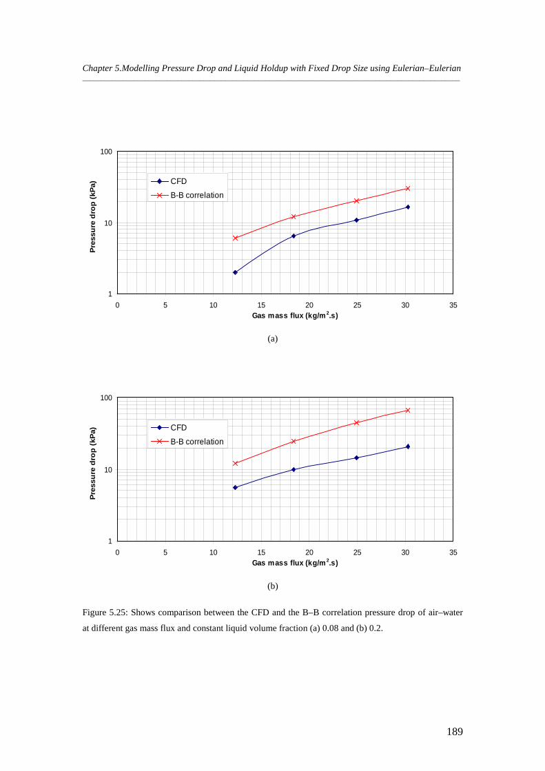
Chapter 5.Modelling Pressure Drop and Liquid Holdup with Fixed Drop Size using Eulerian–Eulerian _______________________________________________________________________________________________________
189
1
10
100
0 5 10 15 20 25 30 35Gas mass flux (kg/m2.s)
Pre
ssu
re d
rop
(kP
a) CFD
B-B correlation
(a)
1
10
100
0 5 10 15 20 25 30 35Gas mass flux (kg/m2.s)
Pre
ssu
re d
rop
(kP
a) CFD
B-B correlation
(b)
Figure 5.25: Shows comparison between the CFD and the B–B correlation pressure drop of air–water
at different gas mass flux and constant liquid volume fraction (a) 0.08 and (b) 0.2.
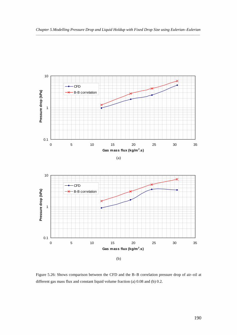
Chapter 5.Modelling Pressure Drop and Liquid Holdup with Fixed Drop Size using Eulerian–Eulerian _______________________________________________________________________________________________________
190
0.1
1
10
0 5 10 15 20 25 30 35
Gas mass flux (kg/m2.s)
Pre
ssu
re d
rop
(kP
a)
CFD
B-B correlation
(a)
0.1
1
10
0 5 10 15 20 25 30 35
Gas mass flux (kg/m2.s)
Pre
ssu
re d
rop
(kP
a)
CFD
B-B correlation
(b)
Figure 5.26: Shows comparison between the CFD and the B–B correlation pressure drop of air–oil at
different gas mass flux and constant liquid volume fraction (a) 0.08 and (b) 0.2.
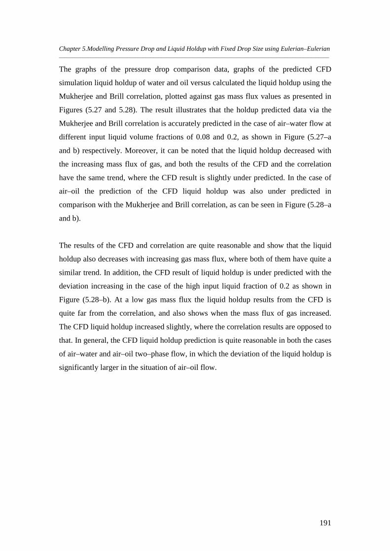
Chapter 5.Modelling Pressure Drop and Liquid Holdup with Fixed Drop Size using Eulerian–Eulerian _______________________________________________________________________________________________________
191
The graphs of the pressure drop comparison data, graphs of the predicted CFD
simulation liquid holdup of water and oil versus calculated the liquid holdup using the
Mukherjee and Brill correlation, plotted against gas mass flux values as presented in
Figures (5.27 and 5.28). The result illustrates that the holdup predicted data via the
Mukherjee and Brill correlation is accurately predicted in the case of air–water flow at
different input liquid volume fractions of 0.08 and 0.2, as shown in Figure (5.27–a
and b) respectively. Moreover, it can be noted that the liquid holdup decreased with
the increasing mass flux of gas, and both the results of the CFD and the correlation
have the same trend, where the CFD result is slightly under predicted. In the case of
air–oil the prediction of the CFD liquid holdup was also under predicted in
comparison with the Mukherjee and Brill correlation, as can be seen in Figure (5.28–a
and b).
The results of the CFD and correlation are quite reasonable and show that the liquid
holdup also decreases with increasing gas mass flux, where both of them have quite a
similar trend. In addition, the CFD result of liquid holdup is under predicted with the
deviation increasing in the case of the high input liquid fraction of 0.2 as shown in
Figure (5.28–b). At a low gas mass flux the liquid holdup results from the CFD is
quite far from the correlation, and also shows when the mass flux of gas increased.
The CFD liquid holdup increased slightly, where the correlation results are opposed to
that. In general, the CFD liquid holdup prediction is quite reasonable in both the cases
of air–water and air–oil two–phase flow, in which the deviation of the liquid holdup is
significantly larger in the situation of air–oil flow.
Chapter 5.Modelling Pressure Drop and Liquid Holdup with Fixed Drop Size using Eulerian–Eulerian _______________________________________________________________________________________________________
192
0
0.05
0.1
0.15
0.2
0.25
0.3
0 5 10 15 20 25 30 35
Gas mass flux (kg/m2.s)
Liq
uid
ho
ldu
p
CFD
M-B correlation
(a)
0
0.05
0.1
0.15
0.2
0.25
0.3
0 5 10 15 20 25 30 35
Gas mass flux (kg/m2.s)
Liq
uid
ho
ldu
p
CFD
M-B correlation
(b)
Figure 5.27: Shows liquid holdup comparison between the CFD simulation and the M–B correlation
results at variant gas mass flux and constant water volume fraction: (a) 0.08 and (b) 0.2.
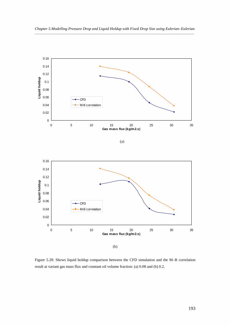
Chapter 5.Modelling Pressure Drop and Liquid Holdup with Fixed Drop Size using Eulerian–Eulerian _______________________________________________________________________________________________________
193
0
0.02
0.04
0.06
0.08
0.1
0.12
0.14
0.16
0 5 10 15 20 25 30 35Gas mass flux (kg/m2.s)
Liq
uid
ho
ldu
p
CFD
M-B correlation
(a)
0
0.02
0.04
0.06
0.08
0.1
0.12
0.14
0.16
0 5 10 15 20 25 30 35Gas mass flux (kg/m2.s)
Liq
uid
ho
ldu
p
CFD
M-B correlation
(b)
Figure 5.28: Shows liquid holdup comparison between the CFD simulation and the M–B correlation
result at variant gas mass flux and constant oil volume fraction: (a) 0.08 and (b) 0.2.
Chapter 5.Modelling Pressure Drop and Liquid Holdup with Fixed Drop Size using Eulerian–Eulerian _______________________________________________________________________________________________________
194
5.13 Conclusions
The following conclusions can be derived based on the results that are achieved from
this investigation:
Various multi–phase turbulence models available in ANYSY FLUENT 12.1 are
applicable to low liquid loading. These models include three high Reynolds number
k–ε models which are standard k–ε, RNG k–ε, and realizable k–ε, and are utilized to
examine the pressure drop in a horizontal pipe. It was found that the RNG k–ε model
is the most appropriate model to predict the pressure drop in comparison with the
experimental data that is available in the literature, and the existing models of Hart et
al. (1989) and Chen et al. (1997). Moreover, a new drag coefficient has been
implemented to account for the drag on a droplet by using the Ishii and Chawla
(1979) expression. There is good quantitative agreement with the experimental data
with the Renormalization Group (RNG) k–ε model for different superficial gas
velocity and a wide range of superficial water velocities. It was observed that the
pressure gradient increased with the system parameters, such as the drop size, water
and gas superficial velocity and the water volume fraction.
The liquid holdup decreased with respect to gas mass flux/superficial velocity, but
increased with the water mass flux/superficial velocity. The deviation of pressure
gradient and liquid holdup obtained throughout the CFD simulation with respect to
the experimental data (Badie et al., 2000) was found to be relatively small at low
superficial gas velocities. Furthermore, when the two empirical correlations that have
been examined (Beggs and Brill (1973), and Mukherjee and Brill (1985)) against the
CFD simulation results of pressure drop and liquid holdup, it was noted that they gave
closer agreement with the air–oil system rather than the air–water system, but shows
reasonable agreement over the entire gas mass flux/superficial velocity.
The pressure drop data for air–water was found to be much higher than for air–oil
systems. This is due to the viscosity difference. It can be concluded that the CFD
simulation, which is more efficient and economic, can be employed as an alternative
to the empirical correlation to obtain the pressure gradient and liquid holdup in two–
Chapter 5.Modelling Pressure Drop and Liquid Holdup with Fixed Drop Size using Eulerian–Eulerian _______________________________________________________________________________________________________
195
phase flow in horizontal pipelines. It is recommended that further investigation of the
pressure drop and liquid holdup prediction be conducted by using a population
balance equation that takes into account the droplet breakage and coalescence.
5.14 Bibliography
ANSYS-FLUENT Inc (2008). FLUENT 12.0, ANSYS-FLUENT Inc, Lebanon, N.H.
Badie, S., C. P. Hale, C. J. Lawrence and G. F. Hewitt (2000). Pressure gradient and
holdup in horizontal two phase gas-liquid flows with low liquid loading.
International Journal of Multiphase Flow, 26, 1525-1543.
Beggs, H. D. and J. P. Brill (1973). A study of two–phase flow in inclined pipes.
Journal of Petroleum Technology, 25, 607-617.
Bel Fdhila, R'Bei (1991). “Analyse experimentale et modeelisation d'un ecoulement
vertical a bulles un elargissement brusque”, PhD thesis, L'Institute National
Polytechnique de Tolouse, Tolouse, France.
Cawkwell, M. G. and M. E. Charles (1985). Pressure, temperature predicted for two-
phase pipelines. Oil and Gas Journal, 85, 101-107.
Chen, X. T., X. D. Cai and J. P. Brill (1997). Gas–liquid stratified-wavy flow in
horizontal pipelines. Journal Energy Resources Technology, 119(2), 209-216.
Chhabra, R. P., S. I. Farooqi and J. F. Richardson (1984). Isothermal Two Phase Flow
of Air and Aqueous Polymer Solutions in a Smooth Horizontal Pipe. Chemical
Engineering Research Design, 62, 22-32.
Chisholm D. (1967). A theoretical basis for the Lockhart-Martinelli correlation for
two-phase flow. International Journal of Heat Mass Transfer, 10, 1767-1778.
Choudhury, D. (1993). Introduction to the renormalization group method and
turbulence modelling. FLUENT Inc. Technical memorandum TM-107.
Fan, Y., Q. Wang, H. Zhang, C. Sarica and T. J. Danielson (2005). A model to predict
liquid holdup and pressure gradient of near-horizontal wet-gas pipelines. The
SPE Annual Technical Conference and Exhibition, Dallas, Texas, 9-12
October.
Ghorai, S. and K. D. P. Nigam (2006). CFD modeling of flow profiles and interfacial
phenomena in two-phase flow in pipes. Chemical Engineering and
Processing, 45(1), 55-65.
Chapter 5.Modelling Pressure Drop and Liquid Holdup with Fixed Drop Size using Eulerian–Eulerian _______________________________________________________________________________________________________
196
Grossetete, C. (1995). “Caraterisation experimentale et simulations de l’evolution
d’un ecoulemnt diphasique a bulles ascendant dans un conduite verticale”,
Collection de notes internes de la Direction des Études et Recherches.
Electricité de France.
Hart, J., P. J. Hamersma and J. M. H. Fortuin (1989). Correlations predicting
frictional pressure drop and liquid holdup during horizontal gas-liquid pipe
flow with a small liquid holdup. International Journal of Multiphase Flow,
15(5), 947-964.
Ishii, M. and T. C. Chawla (1979). Local drag laws in dispersed two-phase flow.
NUREG/CR-1230, ANL-79-105.
Issa, R. I. (1988). Prediction of turbulent, stratified, two-phase flow in inclined pipes
and channels. International Journal of Multiphase Flow, 14(1), 141-154.
Kader, B. A. (1981). Temperature and concentration profiles in fully turbulent
boundary layers. International Journal of Heat and Mass Transfer, 24(9),
1541-1544.
Lahey Jr., R.T., M. Lopez de Bertodano and O.C. Jones Jr. (1993), “Phase distribution
phenomena in complex geometry conduits”, Nuclear Eng. and Design, 141,
177-201.
Lockhart, R. W. and R. C. Martinelli (1949). Proposed correlation of data for
isothermal two-phase, two-component flow in pipes. Chemical Engineering
Progress, 45(1), 39-48.
Mukherjee, H. and J. P. Brill (1985). Pressure drop correlation for inclined two–phase
flow. Journal of Energy Resources Technology, 107, 549-554.
Newton, C. H. and M. Behnia (1998). Numerical calculation of turbulent stratified
gas-liquid pipe flows. International Journal of Multiphase Flow, 24(5), 327-
337.
Olive, N. R., H. -Q. Zhang, Q. Wang, C. L. Redus and J. P. Brill (2003). Experimental
study of low liquid loading gas–liquid flow in near-horizontal pipes. Journal
of Energy Resources Technology, 125, 293-298.
Roscoe, R. and J. Brit (1952). Applied Physics, 3, 267-269.
Shoham, O. and Y. Taitel (1984). Stratified turbulent-turbulent gas-liquid flow in
horizontal and inclined pipes, AIChE Journal, 30(2), 377-385.
Chapter 5.Modelling Pressure Drop and Liquid Holdup with Fixed Drop Size using Eulerian–Eulerian _______________________________________________________________________________________________________
197
Taitel, Y. and A. E. Dukler (1976). Model for predicting flow regime transitions in
horizontal and near horizontal gas–liquid flow. AIChE Journal, 22, 47-55.
Vlachos, N. A., S. A. Paras and A. J. Karabelas (1999). Prediction of holdup, axial
pressure gradient and wall shear stress in wavy stratified and
stratified/atomisation gas/liquid flow. International Journal of Multiphase
Flow, 25(3), 365-376.
Wang, S.K.,S.J. Lee, J. Jones, O. C. and J. Lahey, R. T., "3-D Turbulence Structure
and Phase Distribution Measurements in Bubbly Two-Phase Flows", Int. J.
Multiphase Flow,13, 327-343 (1987).
“Every reasonable effort has been made to acknowledge the owners of copyright
material. I would be pleased to hear from any copyright owner who has been omitted
or incorrectly acknowledged.”
Chapter 6 Prediction of System Parameters and Drop
Size Distribution using CFD and Population
Balance Equation
In the present Chapter, numerical aspects of the coupling between the population of
droplets and the surrounding fluid are exposed. This contribution focuses on the
combined Computational Fluid Dynamics (CFD) and Droplet Population Balance
Model (DPBM), where the DPBM is solved as part of the CFD code.
The droplet population balance equations are solved by the Quadrature Method of
Moments (QMOM). The droplet size distribution in gas–liquid air–water horizontal
co–current annular flow is investigated through a CFD–PBM coupled model. Also the
pressure drop and liquid holdup are obtained and compared with k–ε model of
constant droplet size (presented in Chapter 5) and with an empirical correlation. The
Eulerian–Eulerian k–ε approach is utilized as the framework of this model, and the
population balance equation is used to obtain the dispersed liquid droplet diameter
distribution where the droplet size distribution is investigated in different pipe sizes of
0.0953 and 0.078 m inside diameter. The Turbulent coalescence kernel and Luo's
breakup kernel are used in this investigation.
Chapter 6. Prediction of System Parameters and Drop Size Distribution using CFD–PBM Model ___________________________________________________________________________________
199
6.1 Introduction
A number of different flow regimes can exist for the simultaneous co–current of two–
phase flow in a pipeline. In the transport of two–phase gas–liquid mixtures in a
conduit with a small amount of liquid, the expected flow pattern is characterized by a
wavy interface and drops in the core phase (gas). In this situation, the dynamics of the
film and the liquid droplets is significant in obtaining the pressure drop and liquid
holdup in the conduit (Fore and Dukler, 1995; Simmons and Hanratty, 2001).
The most common flow is annular flow, which can take place at all pipe inclination
angles, and the liquid fraction carried as droplets can differ from zero to one. Droplets
deposit on the wall and form some waves that exist on the liquid film while some
droplets are entrained in the core phase (gas). For a fully developed flow, the liquid
entrained fraction as droplets is illustrated as a balance between the two mechanism
rates of atomisation and deposition. The prediction of such phenomena requires
knowledge of the distribution of droplet sizes in the gas phase (Simmons and
Hanratty, 2001).
The measurement of droplet size in annular flows has been studied by Azzopardi
(1997). Different techniques have been used to find the droplet size distribution.
Tatterson et al. (1977) utilized charge removal from an insulated probe. Wicks and
Dukler (1966) employed a needle bridging technique in which two needles were
placed at a small distance apart and connected to a battery and a resistance. The
droplets larger than the gap completed the circuit and led to an electrical pulse. By
changing the needle gap, the cumulative size distribution was obtained. Semiat and
Dukler (1981) and Lopes and Dukler (1985) utilized a laser grating technique that
generated a local measurement of velocity and droplet size.
The previous techniques were unable to detect small droplets lower than 100 μm.
Therefore, further work has demonstrated that these techniques cause significant error
in measuring the volume median size since a significant proportion of the volume is
carried by small drops with a diameter less than 100 μm. Further refinements were
Chapter 6. Prediction of System Parameters and Drop Size Distribution using CFD–PBM Model ___________________________________________________________________________________
200
made to the laser–grating technique by Fore and Duker (1995). These allowed the
measurement of very small droplet sizes such as 10 μm.
Several measurement techniques which have been used to obtain the droplet size
distribution in horizontal and vertical pipes can be found in Simmon and Hanratty
(2001). For numerical studies, this type of flow pattern (annular) in the horizontal
pipe has received less attention in the literature than other flows such as bubbly flow,
even though this flow is very common in industrial processes such as the transport of
hydrocarbons. Some of the numerical studies that have been conducted in a horizontal
pipe, for example: Ekambara et al. (2008) have employed the two–phase Multiple
Size Group (MUSIG) model to study the internal phase size distribution of horizontal
bubbly flow. In this model, the continuous bubble size distribution is divided into a
series number of discrete size classes.
The mass conservation of each class fraction is balanced using source terms that
describe the inter–fraction mass transfer as a result of bubble coalescence and
breakage processes. Typically, the MUSIG model requires considerable
computational time and resources in order to obtain accurate numerical predictions for
system parameters and size distribution. Dorao et al. (2009) have investigated
numerically the evolution of the droplet size distribution by modelling the interaction
between the droplet and the film based on the statistical method resembling the
population balance equation. They found the distribution of droplet size and a liquid
film are strongly based on entrainment and deposition processes. The numerical
experiments are demonstrated and show the modelling framework principles.
Li et al. (2010) have examined the performance of population balance models using
Average Bubble Number Density technique to predict the phase size distribution,
avoid fraction, interfacial area concentration, and superficial velocity of two–phase
air–water flows in a horizontal pipe. The results obtained have achieved agreement
with the experimental data, but with some inconsistency at specific locations of the
pipe as a result of the insufficient resolution of the turbulent model. They have
Chapter 6. Prediction of System Parameters and Drop Size Distribution using CFD–PBM Model ___________________________________________________________________________________
201
concluded that some challenging issues still need to be addressed in order to improve
the prediction parameters of gas–liquid bubbly flow in a horizontal conduit.
This Chapter presents the population balance equation and the available techniques to
solve it, and also demonstrates the available coalescence and breakage kernels.
Furthermore, the droplet size distribution in gas–liquid horizontal co–current annular
flow is investigated through a CFD in conjunction with population balance model
(PBM) coupled model. A two fluid Eulerian approach is used as the framework of this
model and a population balance equation is used to obtain the dispersed liquid droplet
diameter distribution, pressure drop and liquid holdup of two–phase. Turbulent and
Luo models for coalescence and breakup kernels are utilized in this study.
6.2 Population Balance Equation
In practice, during two–phase flow applications, droplets can break and aggregate due
to droplet–droplet and droplet–fluid interactions. Under these circumstances, a
constant droplet size model might not be suitable for predicting the correct thermo–
fluid dynamics of the gas–liquid two–phase flow. A single droplet size model cannot
properly describe the interfacial interactions that take place between the phases, such
as the mass and heat transfer and interfacial forces. Therefore, in order to develop the
system design and optimization, depending on droplet–film interactions, new
simulation tools are needed to take into account the evolution of the droplet size
distribution resulting from breakage and aggregation or coalescence phenomena in
two–phase flows. Typically, this can be performed using the population balance
modelling framework for illustrating the populations’ evolution of entities (i.e.
droplet, bubble, or particle).
Usually, population balances are encountered in a number of scientific and
engineering disciplines. They are used to study crystallization, polymerization,
precipitation, food processes, particle size distribution (PSD) of crushed material or
dispersed liquid and rain drop formation etc. Although there are a few cases in which
the analytical solutions of population balance equations are available, numerical
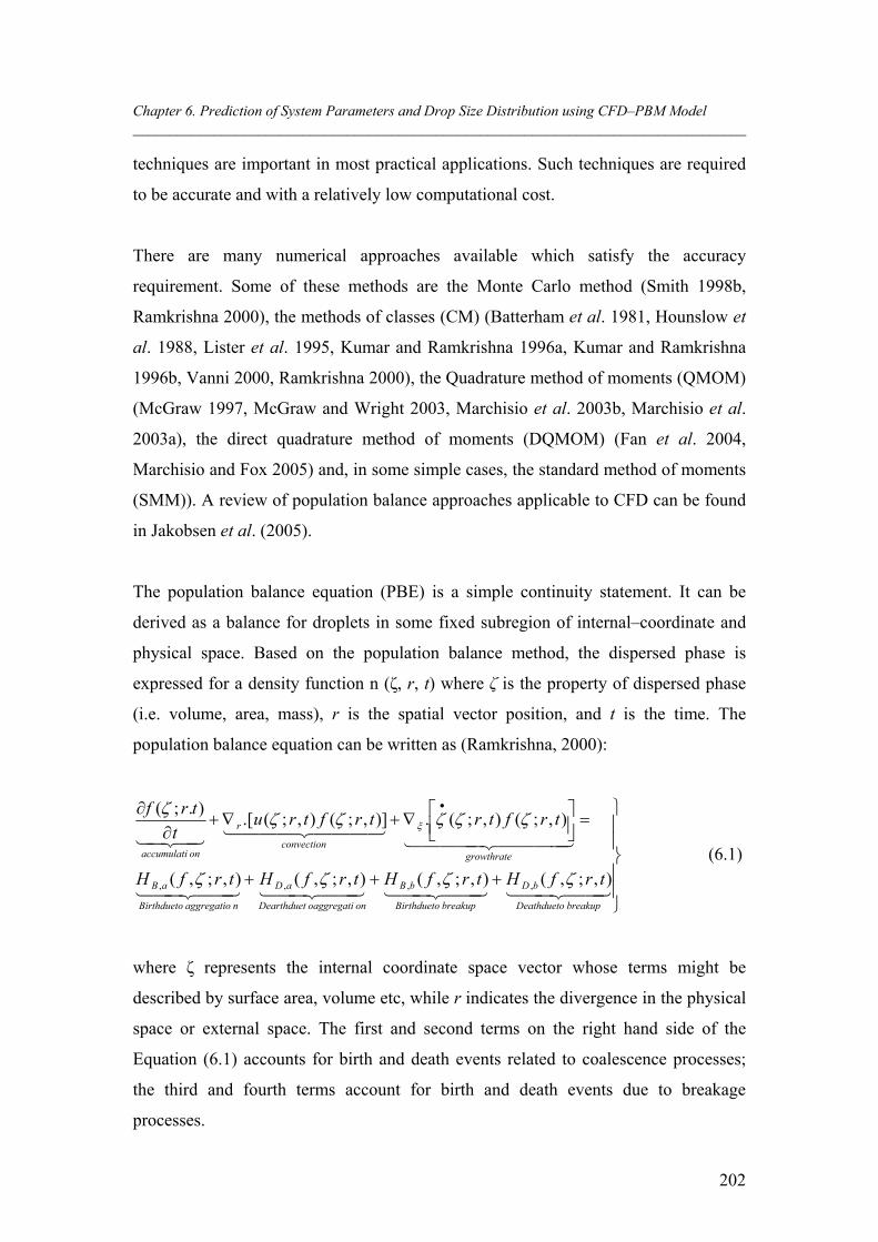
Chapter 6. Prediction of System Parameters and Drop Size Distribution using CFD–PBM Model ___________________________________________________________________________________
202
techniques are important in most practical applications. Such techniques are required
to be accurate and with a relatively low computational cost.
There are many numerical approaches available which satisfy the accuracy
requirement. Some of these methods are the Monte Carlo method (Smith 1998b,
Ramkrishna 2000), the methods of classes (CM) (Batterham et al. 1981, Hounslow et
al. 1988, Lister et al. 1995, Kumar and Ramkrishna 1996a, Kumar and Ramkrishna
1996b, Vanni 2000, Ramkrishna 2000), the Quadrature method of moments (QMOM)
(McGraw 1997, McGraw and Wright 2003, Marchisio et al. 2003b, Marchisio et al.
2003a), the direct quadrature method of moments (DQMOM) (Fan et al. 2004,
Marchisio and Fox 2005) and, in some simple cases, the standard method of moments
(SMM)). A review of population balance approaches applicable to CFD can be found
in Jakobsen et al. (2005).
The population balance equation (PBE) is a simple continuity statement. It can be
derived as a balance for droplets in some fixed subregion of internal–coordinate and
physical space. Based on the population balance method, the dispersed phase is
expressed for a density function n (ζ, r, t) where ζ is the property of dispersed phase
(i.e. volume, area, mass), r is the spatial vector position, and t is the time. The
population balance equation can be written as (Ramkrishna, 2000):
breakupDeathdueto
bD
breakupBirthdueto
bB
onoaggregatiDearthduet
aD
naggregatioBirthdueto
aB
growthrateconvection
r
onaccumulati
trfHtrfHtrfHtrfH
trftrtrftrut
trf
),;,(),;,(),;,(),;,(
),;(),;(.)],;(),;(.[).;(
,,,,
(6.1)
where ζ represents the internal coordinate space vector whose terms might be
described by surface area, volume etc, while r indicates the divergence in the physical
space or external space. The first and second terms on the right hand side of the
Equation (6.1) accounts for birth and death events related to coalescence processes;
the third and fourth terms account for birth and death events due to breakage
processes.
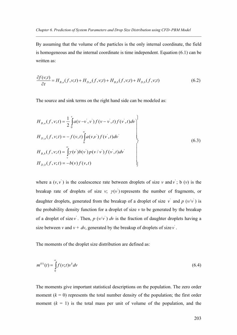
Chapter 6. Prediction of System Parameters and Drop Size Distribution using CFD–PBM Model ___________________________________________________________________________________
203
By assuming that the volume of the particles is the only internal coordinate, the field
is homogeneous and the internal coordinate is time independent. Equation (6.1) can be
written as:
);,();,();,();,();(
,,,, tvfHtvfHtvfHtvfHt
tvfbDbBaDaB
(6.2)
The source and sink terms on the right hand side can be modeled as:
),()();,(
),()/()()();,(
),(),(),();,(
),(),(),(2
1);,(
,
''''',
'''
0
,
'''''
0
,
tvfvbtvfH
dvtvfvvpvbvtvfH
dvtvfvvatvftvfH
dvtvftvvfvvvatvfH
bD
v
bB
aD
v
aB
(6.3)
where a (v, 'v ) is the coalescence rate between droplets of size v and 'v ; b (v) is the
breakup rate of droplets of size v; )( 'v represents the number of fragments, or
daughter droplets, generated from the breakup of a droplet of size 'v and p (v/ 'v ) is
the probability density function for a droplet of size v to be generated by the breakup
of a droplet of size 'v . Then, p (v/ 'v ) dv is the fraction of daughter droplets having a
size between v and v + dv, generated by the breakup of droplets of size 'v .
The moments of the droplet size distribution are defined as:
0
)( );()( dvvtvftm kk (6.4)
The moments give important statistical descriptions on the population. The zero order
moment (k = 0) represents the total number density of the population; the first order
moment (k = 1) is the total mass per unit of volume of the population, and the
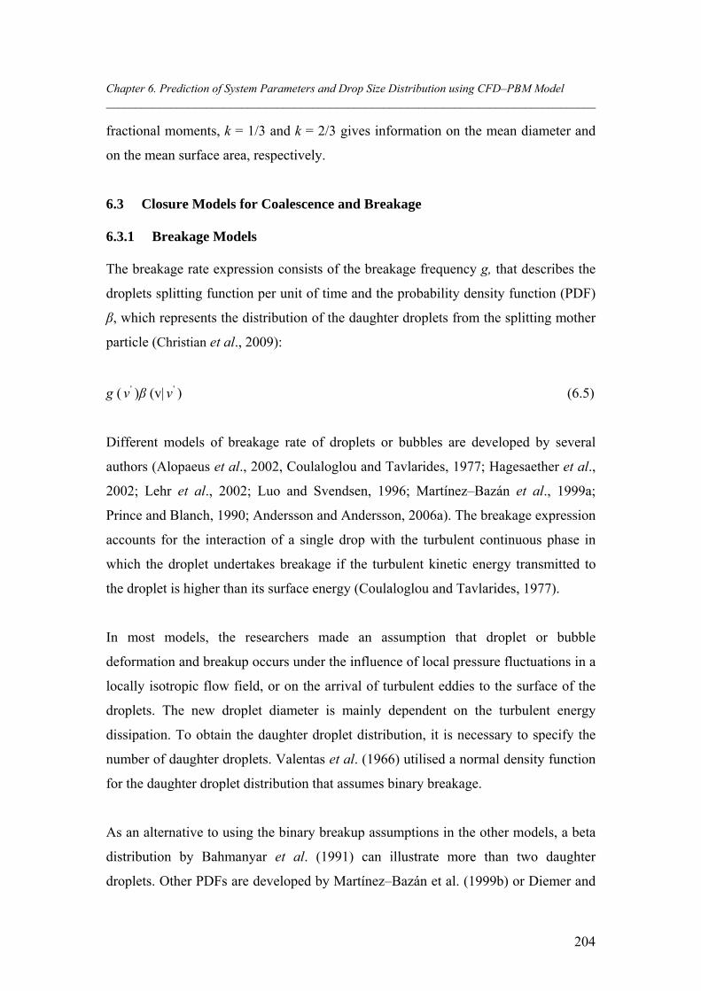
Chapter 6. Prediction of System Parameters and Drop Size Distribution using CFD–PBM Model ___________________________________________________________________________________
204
fractional moments, k = 1/3 and k = 2/3 gives information on the mean diameter and
on the mean surface area, respectively.
6.3 Closure Models for Coalescence and Breakage
6.3.1 Breakage Models
The breakage rate expression consists of the breakage frequency g, that describes the
droplets splitting function per unit of time and the probability density function (PDF)
β, which represents the distribution of the daughter droplets from the splitting mother
particle (Christian et al., 2009):
g ( 'v )β (v| 'v ) (6.5)
Different models of breakage rate of droplets or bubbles are developed by several
authors (Alopaeus et al., 2002, Coulaloglou and Tavlarides, 1977; Hagesaether et al.,
2002; Lehr et al., 2002; Luo and Svendsen, 1996; Martínez–Bazán et al., 1999a;
Prince and Blanch, 1990; Andersson and Andersson, 2006a). The breakage expression
accounts for the interaction of a single drop with the turbulent continuous phase in
which the droplet undertakes breakage if the turbulent kinetic energy transmitted to
the droplet is higher than its surface energy (Coulaloglou and Tavlarides, 1977).
In most models, the researchers made an assumption that droplet or bubble
deformation and breakup occurs under the influence of local pressure fluctuations in a
locally isotropic flow field, or on the arrival of turbulent eddies to the surface of the
droplets. The new droplet diameter is mainly dependent on the turbulent energy
dissipation. To obtain the daughter droplet distribution, it is necessary to specify the
number of daughter droplets. Valentas et al. (1966) utilised a normal density function
for the daughter droplet distribution that assumes binary breakage.
As an alternative to using the binary breakup assumptions in the other models, a beta
distribution by Bahmanyar et al. (1991) can illustrate more than two daughter
droplets. Other PDFs are developed by Martínez–Bazán et al. (1999b) or Diemer and
Chapter 6. Prediction of System Parameters and Drop Size Distribution using CFD–PBM Model ___________________________________________________________________________________
205
Olson (2002). Binary breakup is more appropriate for bubbles but usually not for
droplets in which more than two daughter droplets are formed (Schmidt, 2006). A
review of daughter size distributions and breakage models in the literature can be
found in Wang et al. (2003) and in Lasheras et al. (2002). The experimental
investigation and modelling of breakage phenomena and daughter droplet or bubble
distribution in gas–liquid and liquid–liquid two–phase flow systems is a current
research area (Andersson and Andersson, 2006b; Eastwood et al., 2004; Maaß et al.,
2007; Maaß et al., 2009; Vankova et al., 2007).
6.3.2 Coalescence Models
The process of droplet coalescence takes place due to the interaction between two
droplets and the turbulent continuous phase. The coalescence process among the
droplets is expected to occur if the intervening liquid film has sufficient contact time
to be drained out (Chatzi and Lee, 1987). The coalescence source expressions take
into account the aggregation kernel that considers the probability of successful
collisions between two droplets (v and 'v ). It is usually explained as the result of two
quantities, which are the collision frequency h and the coalescence efficiency λ.
a (v, 'v ) = h (v, 'v ) × λ (v, 'v ) (6.6)
Most of the models are based on the assumption of film drainage (Coulaloglou and
Tavlarides, 1977; Chesters, 1991; Luo (1993), Prince and Blanch (1990), Tsouris and
Tavlarides, 1994). Other methods replaced the film drainage by using a mechanism
derived from the effect of the collision impact (Sovová, 1981) but could not achieve
acceptance. The influence of mass transfer is generally neglected while the droplet–
droplet coalescence is very sensitive to changes in local chemical composition (Simon
and Bart, 2002). Therefore, coalescence phenomena are complicated to tackle, and
there are only a few models in the literature that have a predictive character.
The coalescence mechanism in gas–liquid systems was not fully understood until
recently and is still an important research topic (Eiswirth and Bart, 2008; Henschke et
Chapter 6. Prediction of System Parameters and Drop Size Distribution using CFD–PBM Model ___________________________________________________________________________________
206
al., 2002; Simon, 2004; Tobin and Ramkrishna, 1999). Some of the well known
models, which are available in the literature, such as Coulaloglou and Tavlarides
(1977), Luo and Svendsen (1996), Martínez–Bazán et al. (1999) and Prince and
Blanch (1990), where the Luo and Svendsen (1996) model was applied in this study.
6.4 Numerical Techniques
Analytical solutions of PBEs were presented in some cases where the coalescence and
breakup kernels have a simple form and when the particle size distribution (PSD) has
a specific initial shape (Scott 1968, McCoy and Madras 2003). In some situations the
analytical solution of the PSD is available, but some properties of the PSD, such as
mean diameter and mean surface area, are derived using numerical integration of the
analytical solution. This method computationally is more expensive than solving the
PBE via discretisation approaches. Nevertheless, the analytical solutions can be a
valuable source for validating and testing numerical techniques; it can also be
validated against experimental data, which is considered the easiest way for
validation.
In industrial applications of practical interest, numerical methods are needed to solve
the PBE. The most common techniques employed are the methods of Classes, the
methods of moments, and the Monte Carlo method. Therefore, the three most
common techniques that are available in the CFD application: the standard methods of
moments (SMM), the quadrature method of moments (QMOM), and the discrete
method (DM), will be reviewed.
6.4.1 The Discrete Method
The discrete technique is also called the classes or sectional method, and was
developed by Hounslow et al. (1988), Litster et al. (1995), and Ramkrishna (2000). In
the discrete technique, the entity population (i.e. droplet, bubble or particle) is
discretised into a finite number of size intervals, which describe a set of discrete size
classes or bins. The benefit of this method is robust numerics that lead to discovering
the particle size distribution (PSD) directly. This approach is more valuable when the
Chapter 6. Prediction of System Parameters and Drop Size Distribution using CFD–PBM Model ___________________________________________________________________________________
207
range of particle sizes is identified before and does not span more than two or three
orders of magnitude. In this situation, the particle population can be discretised by a
small number of size intervals and the size distribution, which is combined with fluid
dynamics can be obtained. On the other hand, the disadvantage of this method is that
it is computationally expensive when using a large number of intervals or bins that
must be identified.
The population balance equation (6.1) can be written in terms of droplet size (v) and
volume fraction excluding the growth and nucleation processes.
)().()( ,,,, vDvDvBvBvwvvwvw DBDBVut
(6.7)
where w is the density of water phase and the v is the volume fraction of droplet size
(v), expressed as:
vvv VN where v = 0, 1,… N −1 (6.8)
1
),()(v
v
V
V
v dVtVntN (6.9)
Vv is the volume fraction of droplet size v. The droplet birth and death rates are
described as follows:
'"'"'"
'' '
'"
1 1, vvvvvv
N
v
N
vvvvB xNNaB
(6.10)
'
'
'
1, vv
N
vvvvB NNaD
(6.11)
Chapter 6. Prediction of System Parameters and Drop Size Distribution using CFD–PBM Model ___________________________________________________________________________________
208
N
vvvvvvvD VVNVkB
1,
'
''' )()( (6.12)
vvvD NVkD )(, (6.13)
6.4.2 The Standard Method of Moments
The standard method of moments (SMM) is an effective approach compared to the
discrete population balance approach. The SMM was developed by Randolph and
Larson (1971); it is an alternative method for solving the population balance equation.
In this method, the population balance equation is described via a set of transport
equations that represent the moments of the distribution. The ith moment is identified
by coupling the number density of the entire particle space weighted with the particle
property raised to its ith power.
It is usually sufficient to solve only a few equations of moment, usually between three
to six equations. This can significantly reduce the number of equations to be solved in
contrast with the discretised technique. The advantage of this approach is valuable
when the entire distribution is not required to be presented and certain average and
total quantities are sufficient to characterize the particle distribution. In general, the
first four moments are the most commonly used where the zeroth moment describes
the total number density, the second moment describes the total surface area per unit
volume, and the third moment signifies the total mass density. The disadvantages of
this approach are that exact closure of the right–hand side of Equation (6.1) is
possible only in cases of constant aggregation and size–independent growth, and that
breakage modelling is difficult.
In the SMM approach, assumptions about the size distribution are not needed, and the
moment equations are described with a formula that is created in a closed form
including only the moment’s functions. Nonetheless, the requirement of this exact
closure leads to a serious constraint, where the aggregation term (with the exception
Chapter 6. Prediction of System Parameters and Drop Size Distribution using CFD–PBM Model ___________________________________________________________________________________
209
of the constant aggregation kernel) and breakage phenomena cannot be described as
functions of moments.
The SMM method is derived from taking moments of the PBE with respect to the
internal coordinate of the entity (i.e. M is droplet size). For the homogeneous system,
the ith moment can be written as:
0
);()( dMtMnMtm kk (6.14)
The first four moments (k 0, 1, 2, 3) m0, m1, m2, m3 are the most significant as
mentioned earlier, since they are related to the total number density, the total length,
the total surface area per unit volume, and the total volume density, respectively.
Furthermore, these quantities can be used in this approach to find out the mean
droplet size that can be defined as follows:
0mNtotal (6.15)
1mLtotal (6.16)
2mKA atotal (6.17)
3mKV vtotal (6.18)
2
332 m
md (6.19)
6.4.3 The Quadrature Method of Moments
The quadrature method of moments (QMOM) was developed by McGraw (1997)
when he studied the growth of size–dependence in aerosols. Later it used for
aggregation problems by Barrett and Webb (1998). Wright et al. (2002) have also
Chapter 6. Prediction of System Parameters and Drop Size Distribution using CFD–PBM Model ___________________________________________________________________________________
210
developed a QMOM approach to treat a bivariate aerosol distribution. Furthermore,
the approach was developed for aggregation–breakage processes by Marchisio
(2003a, 2003c). This method has a similar advantage compare to the SMM in terms of
computational costs, but replaces the exact closure needed by SMM with an
approximate closure. This leads to employing the QMOM approach in a wide range of
applications with no limitations. On the other hand, the QMOM approach has a
disadvantage in that it may destroy the shape of the distribution, and information
regarding the distribution is only stored in its moments. The ith moment is described
by integrating the function of population number density with respect to specific
population property, such as droplet sizes, weighted with this property raised to its ith
power. The kth moment can be then identified as:
0
),,(),( dLLtxLntxm kk (6.20)
where L represents the droplet size. When i is equal to zero, it means the zero
moment, which signifies the total number of particles per unit volume, and when the
value of i is equal to three the third moment describing the volume fraction (volume
concentration) of the entities (droplet, bubble, or particle). The QMOM tracks the
population moments, for instance the zero and third moments, instead of its size.
Therefore, it is not based on the minimum and maximum particle sizes; it depends on
the Product–Difference algorithm to obtain weights and abscissas from the moments
that needs the solution of an eigenvalue problem in terms of the population low order
moments.
6.5 Mathematical Modelling
The aim of this investigation is to obtain complete information on the droplet size
distribution and system parameters of two–phase air–water flow in three–dimensional
horizontal pipes. As mentioned in Chapter 3, multiphase CFD models are considered
significant tools that can be used for different chemical and mineral processes. Such a
method utilizes numerical techniques for solving the conservation equations for a
Chapter 6. Prediction of System Parameters and Drop Size Distribution using CFD–PBM Model ___________________________________________________________________________________
211
given flow geometry and boundary conditions. Therefore, using the CFD coupled
with a population balance model for capturing phenomena such as interface
interactions, turbulence for heat and mass transfer, and momentum is seen as relevant
for the particular problem. The governing equations of the flow and the population
balance terms of the coalescence and break–up kernels are described in detail in the
following sections.
6.5.1 Mass Conservation Equation
The numerical simulation is based on the concept of the two fluids Eulerian–Eulerian
model that is derived from the ensemble–average mass and momentum transport
equations for each fluid. The gas phase is considered as a continuum and the liquid
phase (droplets) as the dispersed phase, these equations can be expressed without the
interface mass transfer as follows:
Continuity equation of the gas phase:
0).()(
ggggg ut
(6.21)
Continuity equation of the liquid phase:
iilllill Sfuft
).()( (6.22)
where fi is the volume fraction of droplets of group i (fi = αli / αl) and Si is the source
term, which accounts for the death and birth of droplets as a result of coalescence and
breakage processes. Based on the assumption that is given in Chapter 5 that there is
no mass transfer between two–phase, the term of Si is equal to zero at constant and
uniform droplet size, but in this situation of coalescence and breakage, Si term can be
computed as:
Ci
Bi
Ci
Bii DDBBS where i =1, 2,……, N (6.23)
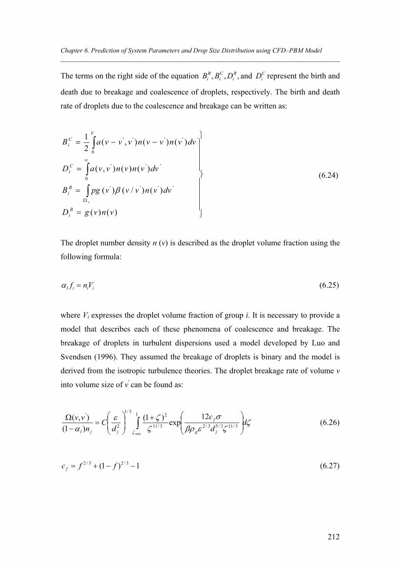
Chapter 6. Prediction of System Parameters and Drop Size Distribution using CFD–PBM Model ___________________________________________________________________________________
212
The terms on the right side of the equation ,,, Bi
Ci
Bi DBB and C
iD represent the birth and
death due to breakage and coalescence of droplets, respectively. The birth and death
rate of droplets due to the coalescence and breakage can be written as:
)()(
)()/()(
)()(),(
)()(),(2
1
''''
0
'''
0
'''''
vnvgD
dvvnvvvpgB
dvvnvnvvaD
dvvnvvnvvvaB
Bi
Bi
Ci
VCi
v
(6.24)
The droplet number density n (v) is described as the droplet volume fraction using the
following formula:
iiil Vnf (6.25)
where Vi expresses the droplet volume fraction of group i. It is necessary to provide a
model that describes each of these phenomena of coalescence and breakage. The
breakage of droplets in turbulent dispersions used a model developed by Luo and
Svendsen (1996). They assumed the breakage of droplets is binary and the model is
derived from the isotropic turbulence theories. The droplet breakage rate of volume v
into volume size of v′ can be found as:
dd
c
dC
n
vv
jg
f
jjl
1
3/113/53/23/11
23/1
2
'
min
12exp
)1(
)1(
),( (6.26)
1)1( 3/23/2 ffc f (6.27)
Chapter 6. Prediction of System Parameters and Drop Size Distribution using CFD–PBM Model ___________________________________________________________________________________
213
where:
ε = the energy dissipation rate per unit of gas mass
ζ = the size ratio between a particle and an eddy in the inertial sub–
range
C and β = empirical constants 0.923 and 2.0, respectively, and are based
on droplet breakage in a turbulent dispersion system
cf = the increase coefficient of surface area
f = the breakage volume fraction
The coalescence of two–droplet is modelled using the turbulent model. The
coalescence process can take place via two methods that are viscous and inertial
subrange mechanisms. The viscous subrange mechanism is used when the particles
sizes are smaller than the Kolmogorov microscale. The collision rate of particles is
influenced by the local shear within the eddy, it is expressed by the Saffman and
Turner (1956) developed relation that can be written as:
8
)(
15
8),(
3ji
Tji
LLLLa
(6.28)
5.0
(6.29)
where T and
represent the pre–factor which accounts for the capture efficiency
coefficient of turbulent collision, and the shear rate, respectively.
The second mechanism of inertial subrange applies in the case where particle sizes are
bigger than the Kolmogorov microscale or smallest eddy. Therefore, they are dragged
via the velocity fluctuations in the flow field. In this situation, the aggregation rate is
described by Abrahamson’s model (1975):
222
2/3
4
)(2),( ji
jiTji UU
LLLLa
(6.30)
Chapter 6. Prediction of System Parameters and Drop Size Distribution using CFD–PBM Model ___________________________________________________________________________________
214
where Ui and Uj are the mean velocity of particle i and j, respectively.
Higshitani et al. (1968) developed relationship for the empirical capture efficiency
coefficient of turbulent collision, which demonstrates the hydrodynamic and attractive
interaction between colliding particles. It can be written as follows:
242.05
732.0
TT N ; NT ≥ 5 (6.31)
where NT describes the ratio between the Van der Waals and the viscous forces, it can
be expressed as:
H
LLN ji
T 8
)(6 3
(6.32)
15
4
(6.33)
where H and
are the Hamaker constant and the deformation rate, respectively.
6.5.2 Momentum Transfer Equations
The momentum conservation of multiphase flows can be described using the volume
averaged momentum equation as follows:
glgggggggggggg Fgpuuut
)().()( (6.34)
where:
ug = the volume averaged velocity vector
p = the pressure
g = the gravity
Chapter 6. Prediction of System Parameters and Drop Size Distribution using CFD–PBM Model ___________________________________________________________________________________
215
τg = the phase shear stress tensor
Fgl = the interface force term between gas and liquid phases
The right hand side expression of Equation (6.34) demonstrates the forces which are
acting on the gas phase. These forces include the pressure gradient, gravity, the
viscous stress term and the interface momentum forces. The pressure is equally
identified in each phase and the effective viscosity of the viscous stress term includes
the laminar viscosity and turbulent component in the turbulence situation. The only
interfacial force considered between the two phases could arise from the drag force in
which other forces are neglected. The cause of drag force is due to the resistance that
is generated by the movement of the body in the gas fluid. Viscous stress produces
skin drag and pressure distribution around the travelling body leading to create a form
drag. The drag force expression can be described in the following form:
)(4
3dcdccdD
dD uuuuC
dF (6.35)
where dp and CD are the droplet diameter and the drag coefficient accounts for the
character of the flow around the droplets, respectively. The drag coefficient has been
modelled using the same expression of the Ishii and Chawla (1976) drag model that is
used in Chapter 5.
6.5.3 Turbulence Equations
Turbulence that is generated by the continuous phase is taken into consideration. The
very common single–phase turbulence models are typically utilized to model the gas
phase turbulence in Eulerian–Eulerian multiphase simulations. In the current study the
RNG k–ε model developed by Choudhury (1993) is employed. The governing
equations for kinetic energy and turbulent dissipation terms are expressed by the
following equations:
Chapter 6. Prediction of System Parameters and Drop Size Distribution using CFD–PBM Model ___________________________________________________________________________________
216
kmbki
ekii
SGGx
k
xku
xk
t
(6.36)
k
GCGk
Cxx
uxt bk
je
ji
i
2*2
31
C
(6.37)
where C1ε and C2ε are the RNG k–ε model constants, which are equal to 1.42, and
1.68, respectively (FLUENT Inc. 2008).
6.6 Method of Solution
The first case of simulation was performed in a three–dimensional horizontal pipe
with dimensions of 0.0953 m ID and 10 m long to examine the CFD–PBM model for
the prediction of drop size distribution and validate that against the experimental data
of Simmons and Hanratty (2001). The rest of the simulations were conducted in the
same pipe size that is used in Chapter 5. The gas phase (air) was considered as a
continuous phase and the liquid phase (water) was considered as a dispersed phase.
For the description of the population balances in the present case the QMOM was
chosen for modelling the drop size distribution where the droplet size ranged from
10–1000 μm.
For the boundary conditions the general method with velocity-inlet at the inlet and
pressure outlet condition at the outlet were applied, but the volume fraction of the
dispersed phase at the inlet was assumed. The surfaces of the upper and the bottom
pipe wall were defined with no–slip wall boundary conditions. All flow conditions at
the inlet were similar to the experiments (Simmons and Hanratty, 2001). The 3D
mesh obtained thus included approximately 936,000 tetrahedral cells.
The computational grid is shown in Figure (6.1). Enhanced wall treatment modeled
the near wall region. The simulations were performed unsteady where the time step
was chosen as 0.001 seconds and is found to be sufficient to produce results
independent of the choice of time step and thus utilized here.
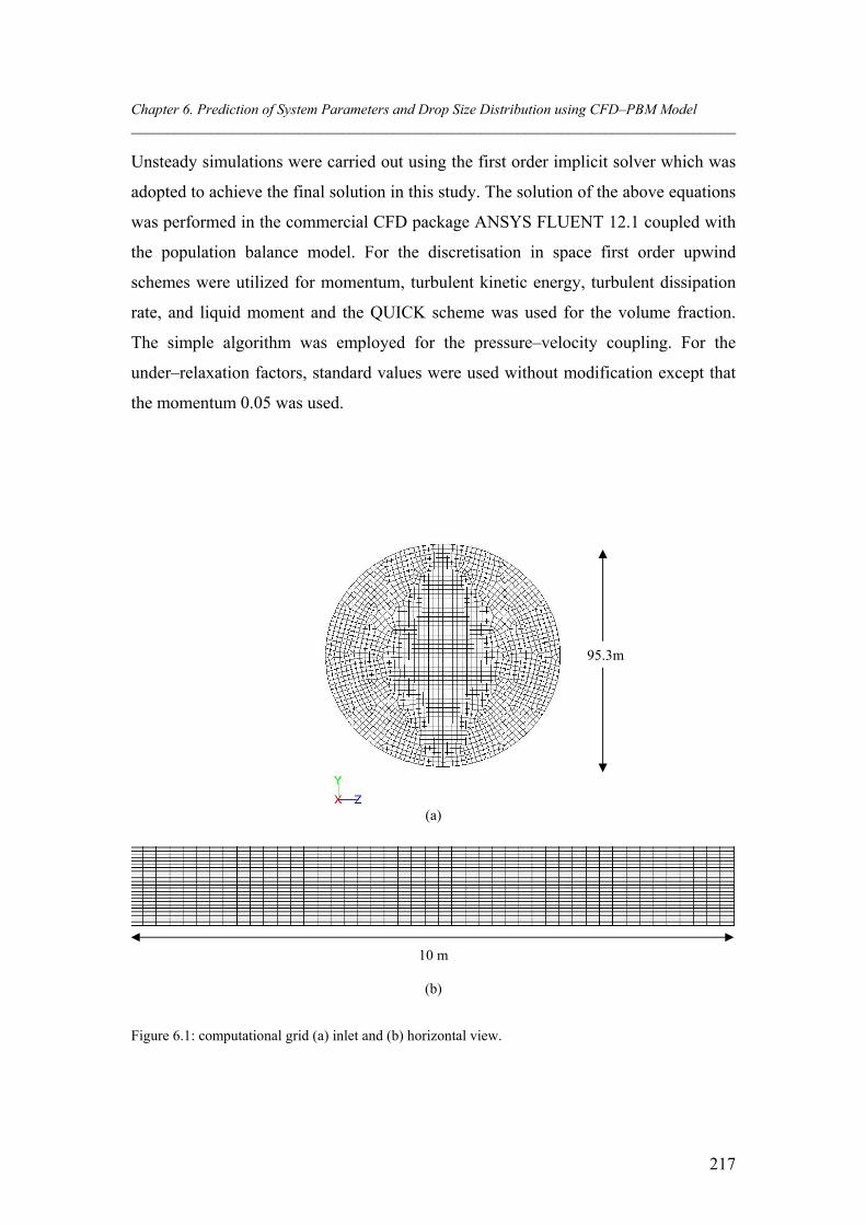
Chapter 6. Prediction of System Parameters and Drop Size Distribution using CFD–PBM Model ___________________________________________________________________________________
217
Unsteady simulations were carried out using the first order implicit solver which was
adopted to achieve the final solution in this study. The solution of the above equations
was performed in the commercial CFD package ANSYS FLUENT 12.1 coupled with
the population balance model. For the discretisation in space first order upwind
schemes were utilized for momentum, turbulent kinetic energy, turbulent dissipation
rate, and liquid moment and the QUICK scheme was used for the volume fraction.
The simple algorithm was employed for the pressure–velocity coupling. For the
under–relaxation factors, standard values were used without modification except that
the momentum 0.05 was used.
(a)
10 m
(b)
Figure 6.1: computational grid (a) inlet and (b) horizontal view.
95.3m
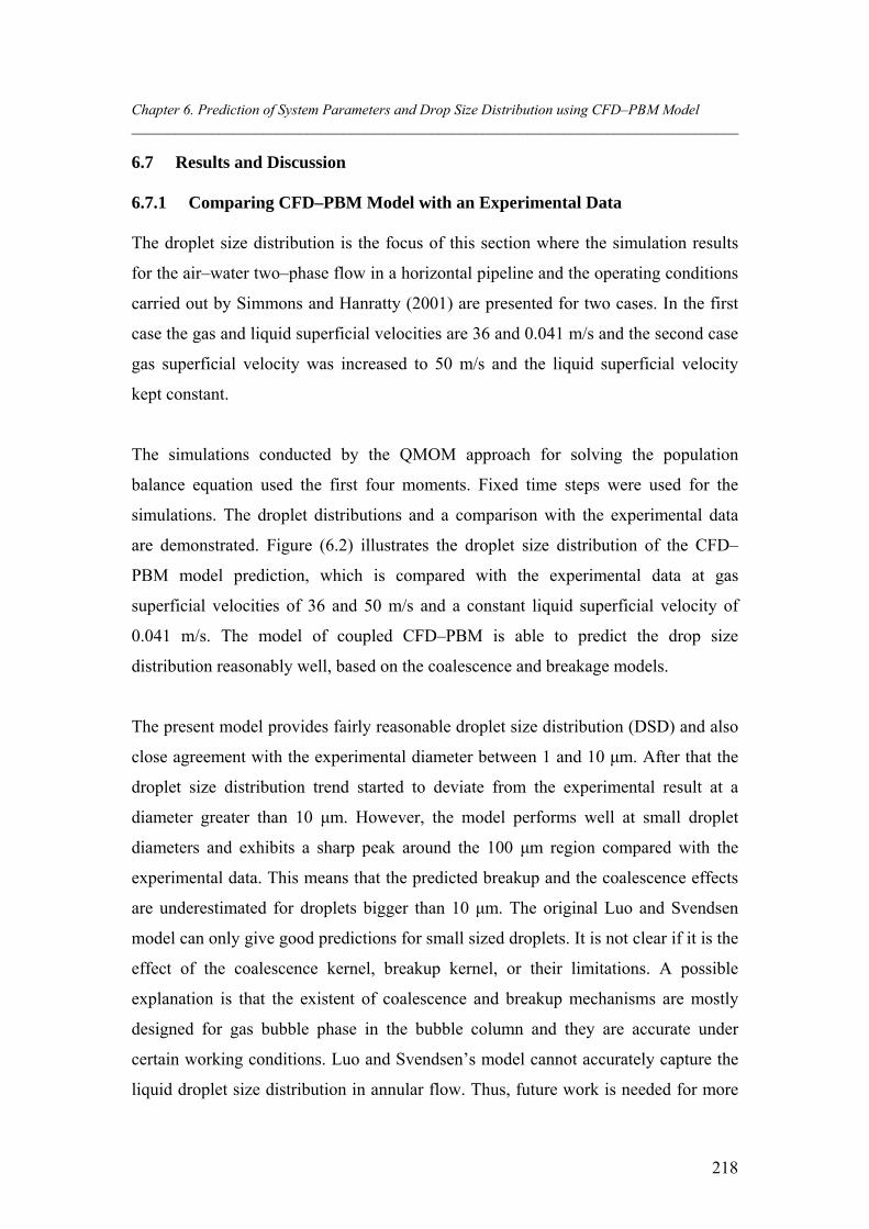
Chapter 6. Prediction of System Parameters and Drop Size Distribution using CFD–PBM Model ___________________________________________________________________________________
218
6.7 Results and Discussion
6.7.1 Comparing CFD–PBM Model with an Experimental Data
The droplet size distribution is the focus of this section where the simulation results
for the air–water two–phase flow in a horizontal pipeline and the operating conditions
carried out by Simmons and Hanratty (2001) are presented for two cases. In the first
case the gas and liquid superficial velocities are 36 and 0.041 m/s and the second case
gas superficial velocity was increased to 50 m/s and the liquid superficial velocity
kept constant.
The simulations conducted by the QMOM approach for solving the population
balance equation used the first four moments. Fixed time steps were used for the
simulations. The droplet distributions and a comparison with the experimental data
are demonstrated. Figure (6.2) illustrates the droplet size distribution of the CFD–
PBM model prediction, which is compared with the experimental data at gas
superficial velocities of 36 and 50 m/s and a constant liquid superficial velocity of
0.041 m/s. The model of coupled CFD–PBM is able to predict the drop size
distribution reasonably well, based on the coalescence and breakage models.
The present model provides fairly reasonable droplet size distribution (DSD) and also
close agreement with the experimental diameter between 1 and 10 μm. After that the
droplet size distribution trend started to deviate from the experimental result at a
diameter greater than 10 μm. However, the model performs well at small droplet
diameters and exhibits a sharp peak around the 100 μm region compared with the
experimental data. This means that the predicted breakup and the coalescence effects
are underestimated for droplets bigger than 10 μm. The original Luo and Svendsen
model can only give good predictions for small sized droplets. It is not clear if it is the
effect of the coalescence kernel, breakup kernel, or their limitations. A possible
explanation is that the existent of coalescence and breakup mechanisms are mostly
designed for gas bubble phase in the bubble column and they are accurate under
certain working conditions. Luo and Svendsen’s model cannot accurately capture the
liquid droplet size distribution in annular flow. Thus, future work is needed for more
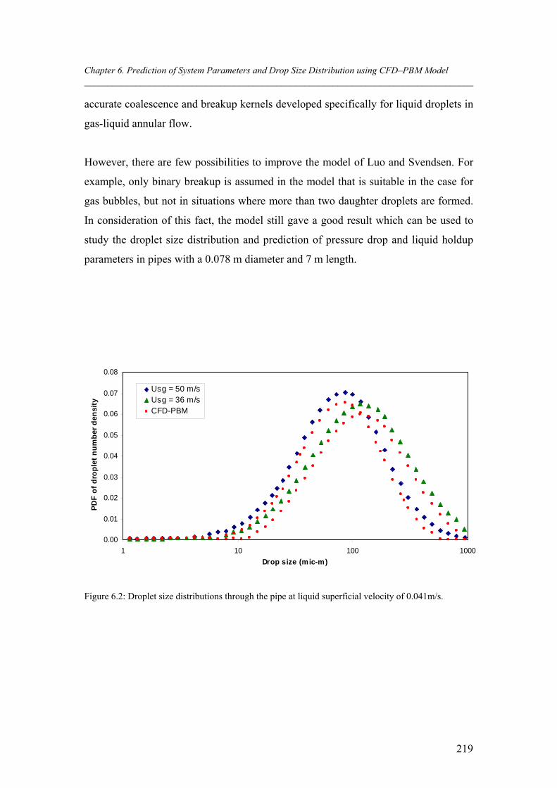
Chapter 6. Prediction of System Parameters and Drop Size Distribution using CFD–PBM Model ___________________________________________________________________________________
219
accurate coalescence and breakup kernels developed specifically for liquid droplets in
gas-liquid annular flow.
However, there are few possibilities to improve the model of Luo and Svendsen. For
example, only binary breakup is assumed in the model that is suitable in the case for
gas bubbles, but not in situations where more than two daughter droplets are formed.
In consideration of this fact, the model still gave a good result which can be used to
study the droplet size distribution and prediction of pressure drop and liquid holdup
parameters in pipes with a 0.078 m diameter and 7 m length.
0.00
0.01
0.02
0.03
0.04
0.05
0.06
0.07
0.08
1 10 100 1000
Drop size (mic-m)
PD
F o
f d
rop
let
nu
mb
er d
ensi
ty
Usg = 50 m/sUsg = 36 m/sCFD-PBM
Figure 6.2: Droplet size distributions through the pipe at liquid superficial velocity of 0.041m/s.
Chapter 6. Prediction of System Parameters and Drop Size Distribution using CFD–PBM Model ___________________________________________________________________________________
220
6.7.2 Effect of Gas Superficial Velocity
6.7.2.1 Droplet Size Distribution (DSD)
Figure (6.3) shows the probability density function (PDF) result for droplet number
density for the present CFD–PBM coupled model in a horizontal pipe with 0.078 m
diameter. The simulated droplet size distribution is plotted at a constant aggregation
and using the aggregation kernel of the turbulent model, where there are constant gas
and liquid velocities of 15 and 0.7 m/s, respectively.
It can be noted that there is a peak in the droplet diameter size, which represents a
balance point between the coalescence and breakup processes. From the perspective
of a liquid droplet, the coalescence is a negative effect for its diameter while the
breakup process is a positive one, and the turbulent effect is the driving force for the
two mechanisms. Different particle size distribution (PSD) has been observed at each
scenario, and differences in the peak of droplet diameter at constant aggregation and
using the aggregation kernel (turbulent model) are around 80 μm and 100 μm,
respectively. Also the PDF of the droplet size was higher than in the case of using
constant aggregation. This means that this scenario does not describe the droplet size
distribution accurately.
Figure (6.4) demonstrates the droplet size distribution at various superficial gas
velocities and a constant superficial liquid velocity of 0.7 m/s. It can be seen that there
is no obvious increase in the small droplet size distribution as the gas superficial
velocity is increased. This shift can be considered less important at medium and high
gas superficial velocity. It can also be noted that there is a clear increase in the
importance of large droplet sizes as the gas superficial velocity increased. The
increase of gas velocity from 20 to 25 m/s does not show any change in the DSD of
the large size (roughly around 900 μm). The CFD–PBM model exhibits the peak of
around 100 μm at a low gas superficial velocity of 15 m/s, which means this drop
diameter is the predominant one in the system.
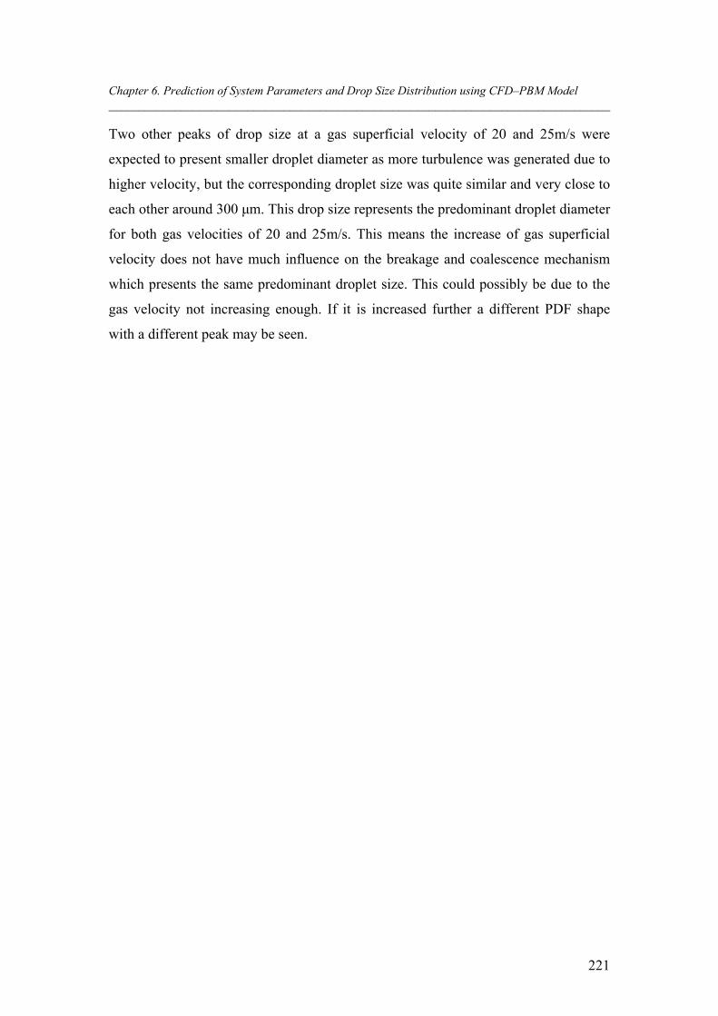
Chapter 6. Prediction of System Parameters and Drop Size Distribution using CFD–PBM Model ___________________________________________________________________________________
221
Two other peaks of drop size at a gas superficial velocity of 20 and 25m/s were
expected to present smaller droplet diameter as more turbulence was generated due to
higher velocity, but the corresponding droplet size was quite similar and very close to
each other around 300 μm. This drop size represents the predominant droplet diameter
for both gas velocities of 20 and 25m/s. This means the increase of gas superficial
velocity does not have much influence on the breakage and coalescence mechanism
which presents the same predominant droplet size. This could possibly be due to the
gas velocity not increasing enough. If it is increased further a different PDF shape
with a different peak may be seen.
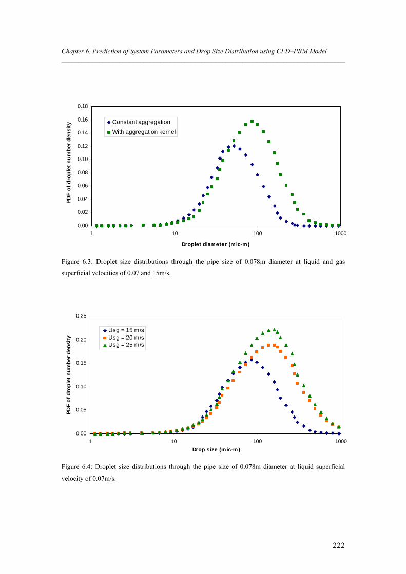
Chapter 6. Prediction of System Parameters and Drop Size Distribution using CFD–PBM Model ___________________________________________________________________________________
222
0.00
0.02
0.04
0.06
0.08
0.10
0.12
0.14
0.16
0.18
1 10 100 1000
Droplet diameter (mic-m)
PD
F o
f d
rop
let
nu
mb
er d
ensi
ty Constant aggregation
With aggregation kernel
Figure 6.3: Droplet size distributions through the pipe size of 0.078m diameter at liquid and gas
superficial velocities of 0.07 and 15m/s.
0.00
0.05
0.10
0.15
0.20
0.25
1 10 100 1000
Drop size (mic-m)
PD
F o
f d
rop
let
nu
mb
er d
ensi
ty
Usg = 15 m/sUsg = 20 m/sUsg = 25 m/s
Figure 6.4: Droplet size distributions through the pipe size of 0.078m diameter at liquid superficial
velocity of 0.07m/s.
Chapter 6. Prediction of System Parameters and Drop Size Distribution using CFD–PBM Model ___________________________________________________________________________________
223
6.7.2.2 Pressure Drop and Liquid Holdup
In contrast with the previous model presented in Chapter 5 of k–ε model of constant
drop size for two–phase flow, in this Chapter the k–ε single drop size model is
Labelled CFD without PBM to be compared with CFD with PBM. The obtained
pressure drop result of two–phase air–water flow was higher in the case of the CFD–
PBM model at a low gas mass flux of 12.5 kg/m2s (corresponding to 10 m/s) and at a
constant input water fraction of 0.08 as shown in Figure (6.5). Therefore, the result of
CFD without PBM pressure drop is deviated from the correlation compared to the
CFD with PBM pressure drop result, which exhibits comparatively less deviation at a
low gas mass flux of 12.5 kg/m2s.
At medium and high gas mass flux of between 18–25 kg/m2s (corresponding to 15–
20m/s), the prediction of pressure drop increased when compared to CFD without
PBM, and became closer to the correlation prediction. At a high gas superficial
velocity of 25m/s (around 32 kg/m2s), the CFD with PBM model pressure drop
prediction is quite similar to the CFD without PBM.
This gives an indication that the predominant droplet diameter into the system is
around 100 μm due to the predicted pressure drop value from both models being
almost comparable. Moreover, as concluded from Figure (6.4) the predominant
droplet size was increased as the gas velocity increased, therefore, the result of the
CFD–PBM model pressure drop at high gas velocity is under predicted. Thus the
current result of pressure drop demonstrates a closer agreement with the correlation
data, particularly at low and medium gas mass fluxes/or superficial velocities for the
CFD with PBM model, where the result showed less deviation compared with the
correlation, although it was slightly higher at CFD without BPM.
The obtained CFD data from the two–phase liquid holdup was plotted against the gas
mass flux, which is treated as a parameter with a constant input water fraction of 0.08
as shown in Figure (6.6). In this figure, it can be observed that the two–phase flow
liquid holdup of the CFD with BPM model has a higher liquid holdup prediction in
comparison with the CFD without PBM model, and the Mukherjee and Brill
Chapter 6. Prediction of System Parameters and Drop Size Distribution using CFD–PBM Model ___________________________________________________________________________________
224
correlation at a low gas mass flux of 12.25 kg/m2s or gas superficial velocity of 10
m/s. At a low gas mass flux we would expect a high amount of liquid holdup, due to
the low turbulence that is generated as a result of low gas phase velocity.
In this situation, the droplets progress to settle down even for small droplet diameters,
but the large droplets require high drag force to push them toward the pipe outlet. This
result might be expected and considered as over prediction at this flow condition;
however the empirical correlation analysis is not able to account for drop size
variation.
At the medium gas mass flux between 18–25 kg/m2s (corresponding to 15–20 m/s),
the two–phase liquid holdup is fluctuating around the empirical correlation result.
Sometimes the predicted liquid holdup of the CFD–PBM model is under and over
prediction, but the predicted liquid holdup data is much closer and less deviated from
the correlation result compared with k–ε of single drop size model. At a higher gas
mass flux above 25 to 30 kg/m2s (corresponding to 20–25 m/s), the CFD–PBM model
predictions agree fully with the results of the Mukherjee and Brill correlation when
compared to the Eulerian–Eulerian model of single droplet diameter.
At high gas velocity we would expect high turbulence and large drag force to be
generated, and this could have a significant influence on the large droplet diameters.
In general, the CFD–PBM model provides close agreement with the empirical
correlation at medium and high gas velocities.
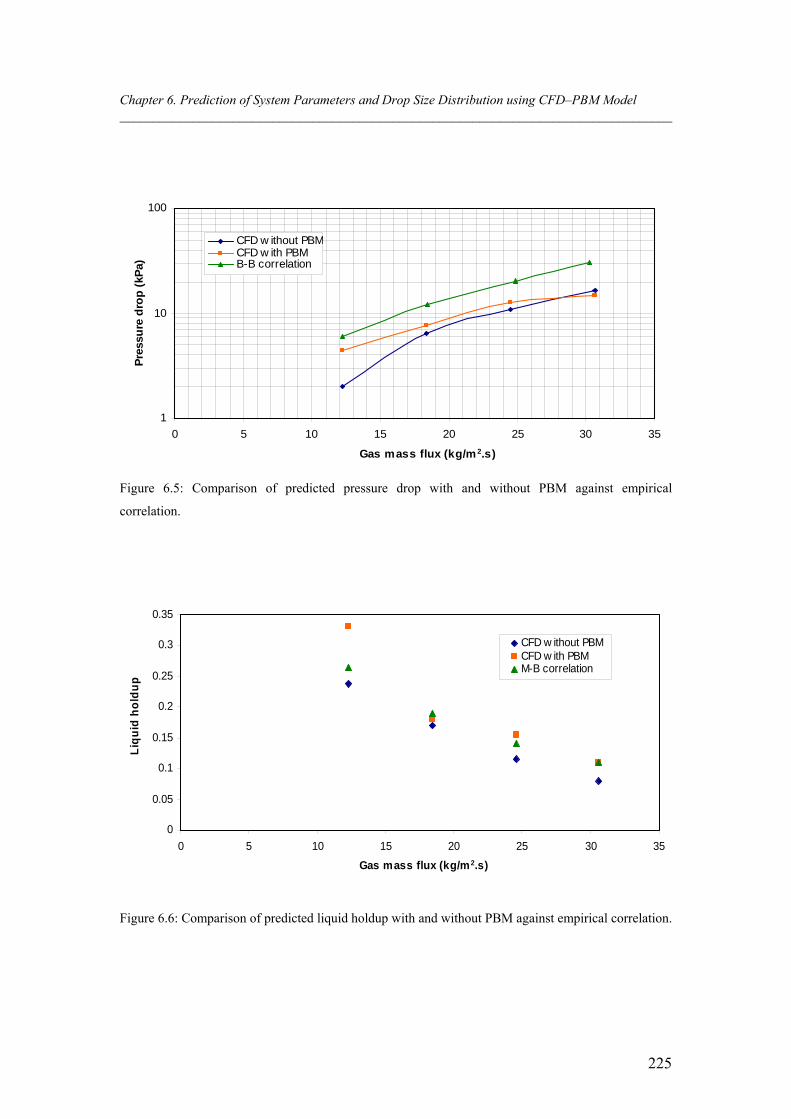
Chapter 6. Prediction of System Parameters and Drop Size Distribution using CFD–PBM Model ___________________________________________________________________________________
225
1
10
100
0 5 10 15 20 25 30 35
Gas mass flux (kg/m 2.s)
Pre
ssu
re d
rop
(kP
a)
CFD w ithout PBMCFD w ith PBMB-B correlation
Figure 6.5: Comparison of predicted pressure drop with and without PBM against empirical
correlation.
0
0.05
0.1
0.15
0.2
0.25
0.3
0.35
0 5 10 15 20 25 30 35
Gas mass flux (kg/m2.s)
Liq
uid
ho
ldu
p
CFD w ithout PBMCFD w ith PBMM-B correlation
Figure 6.6: Comparison of predicted liquid holdup with and without PBM against empirical correlation.
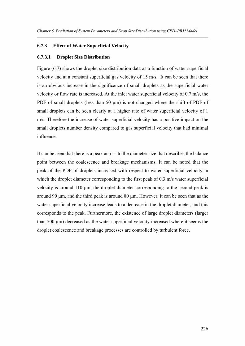
Chapter 6. Prediction of System Parameters and Drop Size Distribution using CFD–PBM Model ___________________________________________________________________________________
226
6.7.3 Effect of Water Superficial Velocity
6.7.3.1 Droplet Size Distribution
Figure (6.7) shows the droplet size distribution data as a function of water superficial
velocity and at a constant superficial gas velocity of 15 m/s. It can be seen that there
is an obvious increase in the significance of small droplets as the superficial water
velocity or flow rate is increased. At the inlet water superficial velocity of 0.7 m/s, the
PDF of small droplets (less than 50 μm) is not changed where the shift of PDF of
small droplets can be seen clearly at a higher rate of water superficial velocity of 1
m/s. Therefore the increase of water superficial velocity has a positive impact on the
small droplets number density compared to gas superficial velocity that had minimal
influence.
It can be seen that there is a peak across to the diameter size that describes the balance
point between the coalescence and breakage mechanisms. It can be noted that the
peak of the PDF of droplets increased with respect to water superficial velocity in
which the droplet diameter corresponding to the first peak of 0.3 m/s water superficial
velocity is around 110 μm, the droplet diameter corresponding to the second peak is
around 90 μm, and the third peak is around 80 μm. However, it can be seen that as the
water superficial velocity increase leads to a decrease in the droplet diameter, and this
corresponds to the peak. Furthermore, the existence of large droplet diameters (larger
than 500 μm) decreased as the water superficial velocity increased where it seems the
droplet coalescence and breakage processes are controlled by turbulent force.
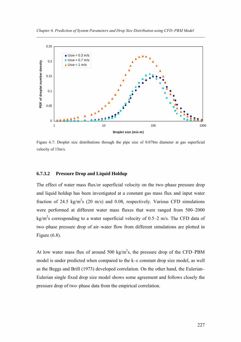
Chapter 6. Prediction of System Parameters and Drop Size Distribution using CFD–PBM Model ___________________________________________________________________________________
227
0
0.05
0.1
0.15
0.2
0.25
1 10 100 1000
Droplet size (mic-m)
PD
F o
f d
rop
let
nu
mb
er d
ensi
ty
Usw = 0.3 m/sUsw = 0.7 m/sUsw = 1 m/s
Figure 6.7: Droplet size distributions through the pipe size of 0.078m diameter at gas superficial
velocity of 15m/s.
6.7.3.2 Pressure Drop and Liquid Holdup
The effect of water mass flux/or superficial velocity on the two–phase pressure drop
and liquid holdup has been investigated at a constant gas mass flux and input water
fraction of 24.5 kg/m2s (20 m/s) and 0.08, respectively. Various CFD simulations
were performed at different water mass fluxes that were ranged from 500–2000
kg/m2s corresponding to a water superficial velocity of 0.5–2 m/s. The CFD data of
two–phase pressure drop of air–water flow from different simulations are plotted in
Figure (6.8).
At low water mass flux of around 500 kg/m2s, the pressure drop of the CFD–PBM
model is under predicted when compared to the k–ε constant drop size model, as well
as the Beggs and Brill (1973) developed correlation. On the other hand, the Eulerian–
Eulerian single fixed drop size model shows some agreement and follows closely the
pressure drop of two–phase data from the empirical correlation.
Chapter 6. Prediction of System Parameters and Drop Size Distribution using CFD–PBM Model ___________________________________________________________________________________
228
At a medium water mass flux of 1000 kg/m2s, the predicted CFD two–phase pressure
drop data of both models with and without PBM are under predicted, compared to the
empirical correlation in which the deviation of the CFD without PBM model is much
less than the CFD with PBM approach.
Both model predictions at low and medium water mass fluxes have similar trends, in
which the two–phase pressure drop is proportional to the water mass flux. At higher
water mass flux above 1500 kg/m2s, an interesting observation for two–phase pressure
drop of CFD with PBM model that is totally deviated from the correlation and rapidly
increased. This increase was significant in comparison with the fixed drop size model,
which exhibits a similar trend to that of the developed correlation of Beggs and Brill
(1973), with a tendency of over prediction compared to the correlation. Moreover, the
CFD without PBM model predicted results are much better with less deviation from
the correlation data as shown in Figure (6.8).
In general, the predicted two–phase pressure drop using two CFD models increases as
water mass flux increases, except at high water mass flux where the CFD–PBM
model is over predicted. This reflects the limitation of the two–phase flow empirical
correlations, which do not take into account the drop size. Again it is important for the
CFD two-phase flows in pipelines to be treated with concern, in particular when using
gas–liquid drag and other forces that could be included. It might also be conducted as
an experimental work in the same pipe size for a better understanding of the two–
phase pressure drop and liquid holdup behaviour.
The other quantity examined with increasing water mass flux is the two–phase liquid
holdup as shown in Figure (6.9). At the inlet water mass flux of 500 kg/m2s, the data
of k–ε with the population balance model are more close to and show less deviation
from the correlation, rather than the k–ε model with a constant drop size. At a medium
of water mass flux of 1000 kg/m2s, the predictions of the CFD liquid holdup data of
the two models are observed to be in close agreement with the correlation, and both
strongly follow the same trend with a slight deviation.
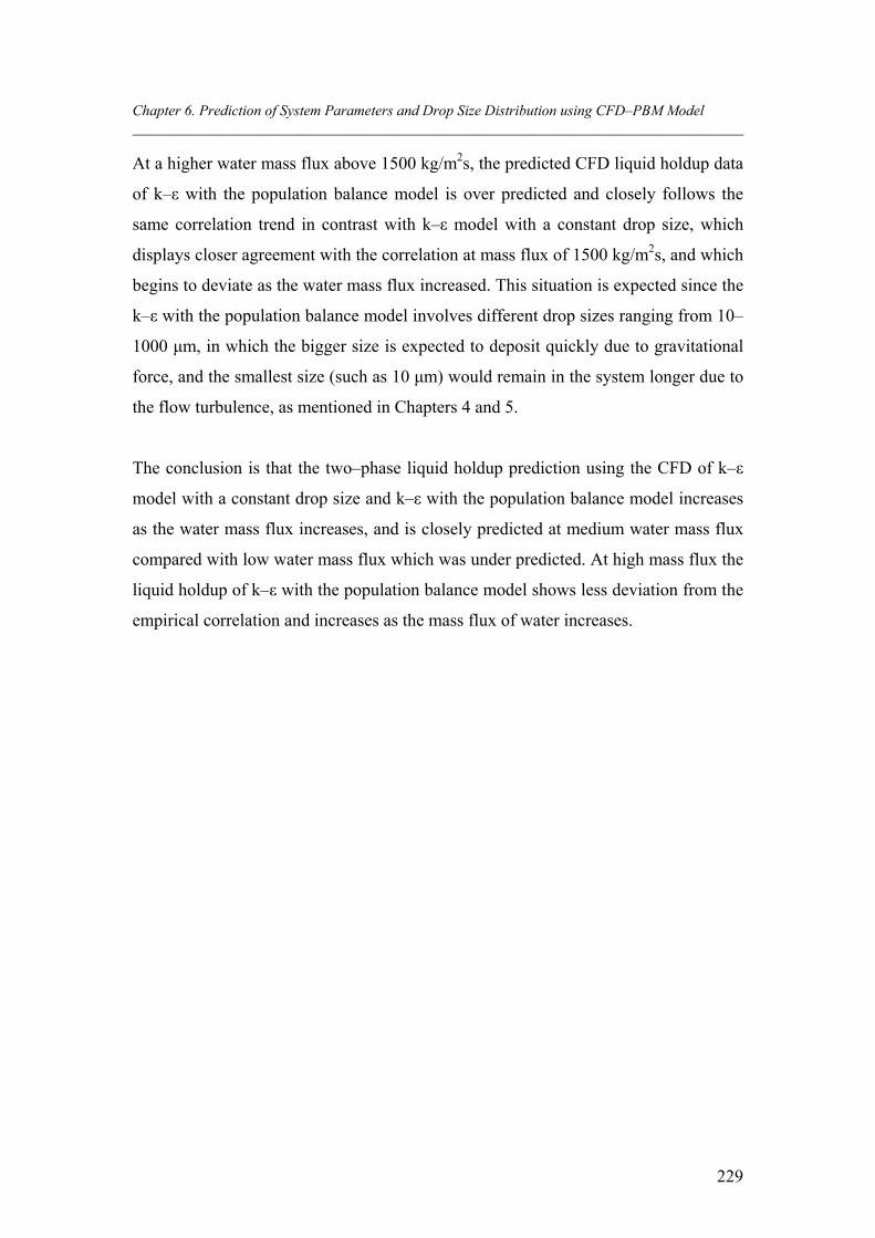
Chapter 6. Prediction of System Parameters and Drop Size Distribution using CFD–PBM Model ___________________________________________________________________________________
229
At a higher water mass flux above 1500 kg/m2s, the predicted CFD liquid holdup data
of k–ε with the population balance model is over predicted and closely follows the
same correlation trend in contrast with k–ε model with a constant drop size, which
displays closer agreement with the correlation at mass flux of 1500 kg/m2s, and which
begins to deviate as the water mass flux increased. This situation is expected since the
k–ε with the population balance model involves different drop sizes ranging from 10–
1000 μm, in which the bigger size is expected to deposit quickly due to gravitational
force, and the smallest size (such as 10 μm) would remain in the system longer due to
the flow turbulence, as mentioned in Chapters 4 and 5.
The conclusion is that the two–phase liquid holdup prediction using the CFD of k–ε
model with a constant drop size and k–ε with the population balance model increases
as the water mass flux increases, and is closely predicted at medium water mass flux
compared with low water mass flux which was under predicted. At high mass flux the
liquid holdup of k–ε with the population balance model shows less deviation from the
empirical correlation and increases as the mass flux of water increases.
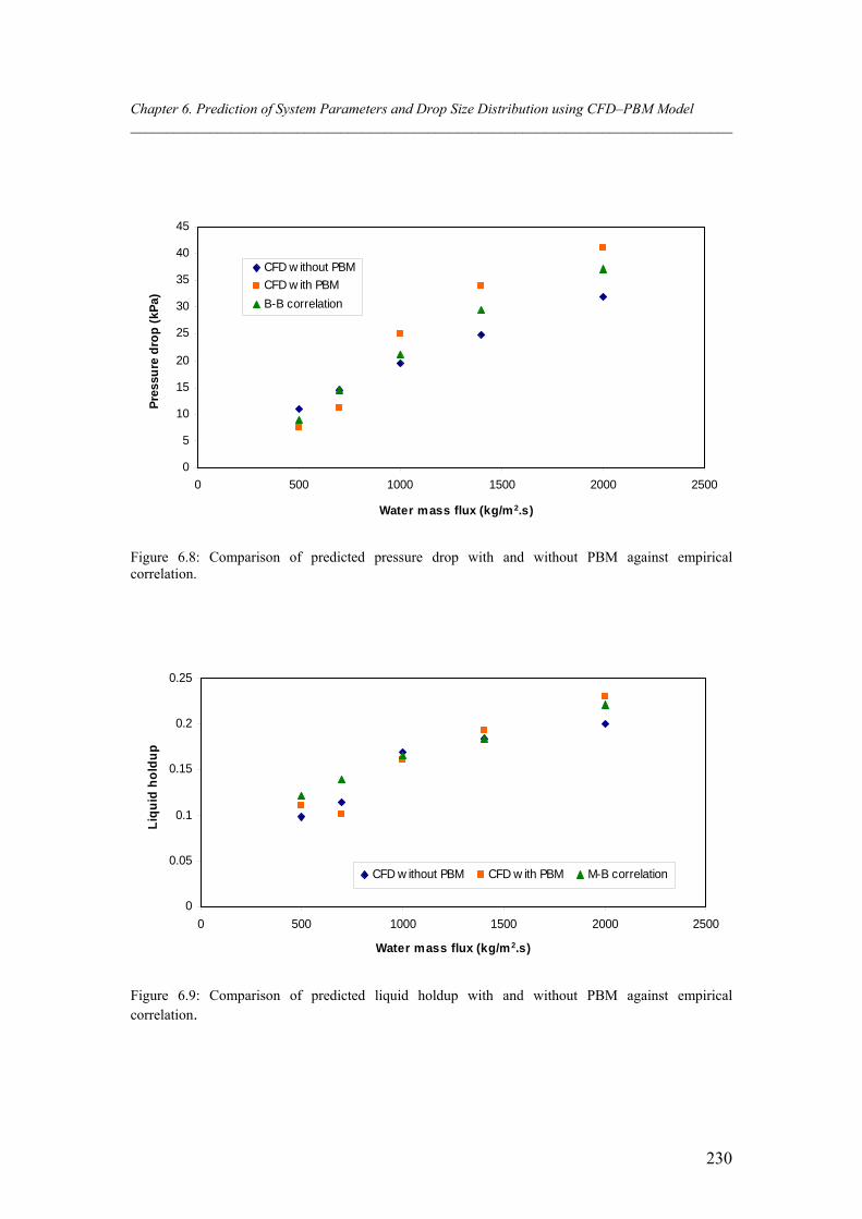
Chapter 6. Prediction of System Parameters and Drop Size Distribution using CFD–PBM Model ___________________________________________________________________________________
230
0
5
10
15
20
25
30
35
40
45
0 500 1000 1500 2000 2500
Water mass flux (kg/m 2.s)
Pre
ssu
re d
rop
(kP
a)
CFD w ithout PBM
CFD w ith PBM
B-B correlation
Figure 6.8: Comparison of predicted pressure drop with and without PBM against empirical correlation.
0
0.05
0.1
0.15
0.2
0.25
0 500 1000 1500 2000 2500
Water mass flux (kg/m2.s)
Liq
uid
ho
ldu
p
CFD w ithout PBM CFD w ith PBM M-B correlation
Figure 6.9: Comparison of predicted liquid holdup with and without PBM against empirical correlation.
Chapter 6. Prediction of System Parameters and Drop Size Distribution using CFD–PBM Model ___________________________________________________________________________________
231
6.8 Conclusions
In this Chapter, a CFD–PBM coupled model in the framework of ANSYS FLUENT
12.1 was intended to investigate the droplet’s size distribution in a gas–liquid air–
water annular flow system. Two phases are modeled by the Eulerian–Eulerian method
and the turbulence is accounted for by a renormalization group k–ε model. For the
solution of PBE, the Quadrature Method of Moments is used and particular
coalescence and breakup kernels were utilized to demonstrate the droplet size
distribution behaviour. The flow variables, such as gas and liquid superficial
velocities are employed to examine the k–ε with population balance model for
predicting the two–phase pressure drop and liquid holdup.
The results of using k–ε with the population balance model illustrate that the
numerical prediction of droplet size distribution in annular flow using traditional
coalescence and breakup kernels is possible. The results suggest that using the
turbulent model and the Luo and Svendsen model for the aggregation and breakage
kernel shows reasonable performance compared with the Simmons and Henratty
(2001) experimental data covering all diameter ranges in the present investigation.
The CFD–PBM model shows good predictions for small sized droplets. It is clear that
the use of two models of the coalescence and breakage kernels leads to presentation of
a reasonable result. Luo and Svendsen’s model and turbulent model could not
precisely capture the liquid droplet size distribution in annular flow. Therefore,
further work is required for more accurate coalescence and breakup kernels developed
specifically for liquid droplets in gas–liquid annular flow.
A comparison of computational data of k–ε model of constant droplet size and the
CFD–PBM approach for the prediction of two–phase pressure drop and liquid holdup
has been made. Also the computational data were compared with an empirical
correlation reported in the literature. The pipe simulations were performed with a
different mass flux of two–phase and constant input volume fraction of dispersed
phase. The CFD–PBM model shows that the two–phase pressure drop and liquid
holdup as well increase as the superficial velocity of air and water increase.
Moreover, the gas and liquid mass flux had significant influence on the pressure drop,
Chapter 6. Prediction of System Parameters and Drop Size Distribution using CFD–PBM Model ___________________________________________________________________________________
232
and led to a rapid increase. In comparison with the single drop size model, the
pressure drop data were lower than the CFD–PBM approach. The liquid holdup was
also increased but at high mass flux rather than at low mass flux.
It can be concluded that this study showed that the introduced CFD–PBM model can
lead to a reasonable prediction for two–phase pressure drop and liquid holdup
compared to the k–ε model with a constant drop size, and gives a better understanding
for the two–phase flow pressure drop and liquid holdup behaviour. However, in order
to obtain more reliable CFD simulation data relating to droplet size distribution,
pressure drop and liquid holdup of two–phase flow, an experimental work using the
same pipe size dimensions to validate the data more accurately, rather than using an
empirical correlation which provides a reasonable indication to the system
parameters, is required.
6.9 Bibliography
Abrahamson, J. (1975). Collision Rates of Small Particles in a Vigourously Turbulent
Fluid. Chemical Engineering Science, 30, 1371-1379.
Alopaeus, V., J. Koskinen and K. I. Keskinen (2002). Simulation of the population
balances for liquid-liquid systems in a nonideal stirred tank. Part 2 Parameter
fitting and the use of the multiblock model for dense dispersions. Chemical
Engineering Science, 57, 1815-1825.
Andersson, R. and B. Andersson (2006a). Modeling the breakup of fluid particles in
turbulent flows. AIChE Journal, 52 (6), 2031-2038.
Andersson, R. and B. Andersson (2006b). On the breakup of fluid particles in
turbulent flows. AIChE Journal, 52 (6), 2020-2030.
Azzopardi, B. J. (1997). Drops in annular two–phase flow. International Journal of
Multiphase Flow, 23, 1-53.
Bahmanyar, H. and M. J. Slater (1991). Studies of drop-break-up in liquid-liquid
systems in a rotating disc contactor part I: conditions of no mass transfer.
Chemical Engineering Technology, 14, 79-89.
Chapter 6. Prediction of System Parameters and Drop Size Distribution using CFD–PBM Model ___________________________________________________________________________________
233
Barrett, J. C. and N. A. Webb (1998). A comparison of some approximate methods
for solving the aerosol general dynamic equation. Journal of Aerosol Science,
29, 31-39.
Batterham, R. J., J. S. Hall and G. Barton (1981). Pelletizing kinetics and simulation
of full-scale balling circuits. In: 3rd International Symposium on
Agglomeration, Nürnberg, Germany, 136 (A).
Chatzi, E. and J. L. Lee (1987). Analysis of interaction for liquid-liquid dispersion in
agitated vessels. Industrial & Engineering Chemistry Research, 26, 2263-
2267.
Chesters, A. K. (1991). The modelling of coalescence processes in fluid-liquid
dispersions. A review of current understanding. Trans IChemE, 69 (A), 259-
281.
Choudhury D. (1993). Introduction to the renormalization group method and
turbulence modelling. Fluent Inc. Technical memorandum TM-107.
Christian D., M. M. Attarakih and H. -J. Bart (2009). Coupling of CFD with DPBM
for an RDC extractor. Chemical Engineering Science, 64, 721-732.
Coulaloglou, C. A. and L. L. Tavlarides (1977). Description of interaction processes
in agitated liquid-liquid dispersions. Chemical Engineering Science, 32, 1289-
1297.
Diemer, R. B. and J. H. Olson (2002). A moment methodology for coagulation and
breakage problems: Part 3- generalized daughter distribution functions.
Chemical Engineering Science, 57, 4187-4198.
Dorao, C. A., M. Fernandino, L. E. Patruno, P. M. Dupuy, H. A. Jakobsen and H. F.
Svendsen (2009). Macroscopic description of droplet–film interaction for gas–
liquid systems. Applied Mathematical Modelling Journal, 33 (8), 3309-3318.
Eastwood, C. D., L. Armi and J. C. Lasheras (2004). The breakup of immiscible fluids
in turbulent flows. Journal of Fluid Mechanics 502, 309-333.
Eiswirth, R. T. and H. -J. Bart (2008). Experimental investigation of droplet-droplet
coalescence in liquid-liquid systems. Proceeding International Solvent
Extraction Conference ISEC 2008, Moyer, B. (Edition), Canadian Institute of
Mining, Metallurgy and Petroleum, Montreal, 2, 1177-1182.
Chapter 6. Prediction of System Parameters and Drop Size Distribution using CFD–PBM Model ___________________________________________________________________________________
234
Ekambara, K., R. S. Sanders, K. Nandakumar and J. H. Masliyah (2008). CFD
simulation of bubbly two–phase flow in horizontal pipes. Chemical
Engineering Journal, 144, 277-288.
Fan, R., D. L. Marchisio and R. O. Fox (2004). Application of the direct quadrature
method of moments to polydisperse gas-solid fluidized beds. Journal of
Aerosol Science 139, 7-20.
Fore, L. B. and A. E. Dukler (1995). Distribution of drop size and velocity in gas–
liquid annular flow. International Journal of Multiphase Flow, 21 (2), 137-
149.
Hagesaether, L. (2002). Coalescence and break-up of drops and bubbles. PhD thesis,
Norwegian University of Science and Technology, Trondheim, Norway.
Henschke, M., L. H. Schlieper and A. Pfennig (2002). Determination of coalescence
parameter from batch-settling experiments. Chemical Engineering Journal, 85
(2), 369-378.
Higashitani, K., K. Yamauchi, Y. Matsuno and G. Hosokawa (1983). Turbulent
coagulation of particles dispersed in a viscous fluid. Chemical Engineering
Journal Japan, 16 (4), 299-304.
Hounslow, M. J., R. L. Ryall and V. R. Marshall (1988). A discretized population
balance for nucleation, growth and aggregation. AIChE Journal, 34 (11),
1821-1832.
Hounslow, M. J., R. L. Ryall and V. R. Marshall (1988). A discretized population
balance for nucleation, growth, and aggregation. AIChE Journal, 34 (11),
1821-1832.
Ishii, M. and T. C. Chawla (1979). Local drag laws in dispersed two-phase flow,
NUREG/CR-1230, ANL-79-105.
Jakobsen, H. A., H. Lindborg and C. A. Dorao (2005). Modeling of bubble column
reactors: progress and limitations. Industrial and Chemical Engineering
Research, 44 (14), 5107-5151.
Kumar, S. and D. Ramkrishna (1996a). On the solution of population balance
equations by discretization-i. a fixed pivot technique. Chemical Engineering
Science 51 (8), 1311–1332.
Chapter 6. Prediction of System Parameters and Drop Size Distribution using CFD–PBM Model ___________________________________________________________________________________
235
Kumar, S. and D. Ramkrishna (1996b). On the solution of population balance
equations by discretization-ii. a moving pivot technique. Chemical
Engineering Science 51(8), 1333–1342.
Lasheras, J. C., C. Eastwood, C. Martínez-Bazán and J. L. Montañés (2002). A review
of statistical models for the break-up of an immiscible fluid immersed into a
fully developed turbulent flow. International Journal of Multiphase Flow, 28,
247-278.
Lehr, F., M. Millies and D. Mewes (2002). Bubble-size distributions and flow fields
in bubble columns. AIChE Journal, 48, 2426-2442.
Li, C., G. H. Yeoh, S. C. P. Cheung and J. Y. Tu (2010). On modelling horizontal
gas–liquid flow using population balance approach, 17th Australian Fluid
Mechanics Conference, Auckland, 5-9 December.
Lister, J. D., D. J. Smith and M. J. Hounslow (1995). Adjustable discretized
population balance for growth and aggregation. AIChE Journal, 41(3), 591-
603.
Litster, J. D., D. J. Smit and M. J. Hounslow (1995). Adjustable discretization
population balance for growth and aggregation. AIChE Journal, 41 (3), 591-
603.
Lopes, J. C. B. and A. E. Dukler (1985). Droplet sizes dynamics and deposition in
vertical annular flow. US Nuclear Regulatory Commission, Washington DC,
USA, Report NUREG/CR-4424.
Luo, H. (1993). Coalescence, breakup and liquid circulation in bubble column
reactors. PhD thesis, University of Trondheim, Norway.
Luo, H. and H. F. Svendsen (1996). Theoretical model for drop and bubble breakup in
turbulent dispersions. AIChE Journal, 42, 1225-1233.
Maaß, S., A. Gäbler, A. Zaccone, A. R. Paschedag and M. Kraume (2007).
Experimental investigations and modelling of breakage phenomena in stirred
liquid/liquid systems. Chemical Engineering Research and Design, 85, 703-
709.
Maaß, S., S. Wollny, R. Sperling and M. Kraume (2009). Numerical and experimental
analysis of particle strain and breakage in turbulent dispersions. Chemical
Engineering Research and Design, 87, 565-572.
Chapter 6. Prediction of System Parameters and Drop Size Distribution using CFD–PBM Model ___________________________________________________________________________________
236
Marchisio, D. L. and R. O. Fox (2005). Solution of population balance equations
using the direct quadrature method of moments. Journal of Aerosol Science
36(1), 43-73.
Marchisio, D. L., J. T. Pikturna, R. O. Fox and R. D. Vigil (2003a). Quadrature
method of moments for population balance equations. AIChE Journal, 49(5),
1266-1276.
Marchisio, D. L., R. D. Vigil and R. O. Fox (2003b). Quadrature method of moments
for aggregation-breakage processes. Journal of Colloid and Interface Science,
258, 322-334.
Marchisio, D. L., R. O. Fox and R. D. Vigil (2003c). Implementation of the
quadrature method of moments in CFD codes for aggregation-breakage
problems. Chemical Engineering Science, 58, 3337-33351.
Martínez-Bazán, C., J. L. Montañés and J. C. Lasheras (1999a). On the breakup of an
air bubble injected into a fully developed turbulent flow. Part 1. breakup
frequency. Journal of Fluid Mechanics, 401, 157-182.
McCoy, B. J. and G. Madras (2003). Analytical solution for a population balance
equation with aggregation and fragmentation. Chemical Engineering Science,
58, 3049-3051.
McGraw, R. (1997). Description of aerosol dynamics by the quadrature method of
moments. Aerosol Science and Technology, 27, 255-265.
McGraw, R. and D. L. Wright (2003). Chemically resolved aerosol dynamics for
internal mixtures by the quadrature method of moments. Journal of Aerosol
Science, 34, 189-209.
Prince, M. J. and H. W. Blanch (1990). Bubble coalescence and break-up in air-
sparged bubble columns. AIChE Journal, 36, 1485-1499.
Ramkrishna, D. (2000). Population balances. Academic Press. San Diego.
Randolph, A. D. and M. A. Larson (1971). Theory of Particulate Processes: Analysis
and Techniques of Continuous Crystallization. Academic Press, San Diego,
CA.
Saffman, P. G. and J. S. Turner (1956). On the collision of droplets in turbulent
clouds. Journal of Fluid Mechanics, 1, 16-30.
Chapter 6. Prediction of System Parameters and Drop Size Distribution using CFD–PBM Model ___________________________________________________________________________________
237
Schmidt, S. A. (2006). Populations dynamische Simulation gerührter
Extraktionskolonnen auf der Basis von Einzeltropfen-und
Tropfenschwarmuntersuchungen. Dr.-Ing. Thesis, Shaker Verlag, Aachen.
Scott, W. T. (1968). Analytic studies of cloud droplet coalescence i. Journal of the
Atmospheric Science, 25, 54-65.
Semiat, R. and A. E. Dukler (1981). Simultaneous measurement of size and velocity
of bubbles and drops: a new optical technique. American Institute of Chemical
Engineering Journal, 27, 148-159.
Simmons, M. J. H. and T. J. Hanratty (2001). Droplet size measurements in horizontal
annular gas–liquid flow. International Journal of Multiphase Flow, 27(5),
861-883.
Simon, M. (2004). Koaleszenz von Tropfen und Tropfenschwärmen. Dr.-Ing. Thesis,
TU Kaiserslautern, Kaiserslautern.
Simon, M. and H. -J. Bart (2002). Experimental studies of coalescence in liquid-liquid
systems. Chemical Engineering Technology, 25, 481-484.
Smith, M. (1998b). Constant-number monte carlo simulation of population balances.
Chemical Engineering Science, 53(9), 1777-1786.
Sovova, H. (1981). Breakage and coalescence of drops in a batch stirred vessel–II.
Comparison of model and experiments. Chemical Engineering Science, 36,
1567-1573.
Tatterson, D. F., J. C. Dallman and T. J. Hanratty (1977). Drop sizes in annular gas–
liquid flow. AIChE Journal, 23, 68-76.
Tobin, T. and D. Ramkrishna (1999). Modeling the effect of drop charge in turbulent
liquid-liquid dispersions. Canadian Journal of Chemical Engineering, 77,
1090-1104.
Tsouris, C. and L. L. Tavlarides (1994). Breakage and coalescence models for drops
in turbulent dispersions. AIChE Journal, 40, 395-406.
Valentas, K.J. and N. R. Amundson (1966). Breakage and coalescence in dispersed
phase systems. Industrial & Engineering Chemistry Fundamentals, 5, 533-
542.
Chapter 6. Prediction of System Parameters and Drop Size Distribution using CFD–PBM Model ___________________________________________________________________________________
238
Valentas, K.J., O. Bilous and N. R. Amundson (1966). Analysis of breakage in
dispersed phase systems. Industrial & Engineering Chemistry Fundamentals,
5, 271-279.
Vankova, N., S. Tcholakova, N. D. Denkov, V. D. Vulchev and T. Danner (2007).
Emulsifiaction in turbulent flow 2. Breakage rate constants. Journal of Colloid
and Interface Science, 313, 612-629.
Vanni, M. (2000). Approximate population balance equations for aggregation
breakage processes. Journal of Colloid and Interface Science, 221, 143–160.
Wang, T., J. Wang and Y. Jin (2003). A novel theoretical breakup kernel function for
bubbles/droplets in a turbulent flow. Chemical Engineering Science, 58, 4629-
4637.
Wicks, M. and A. E. Dukler (1966). In-situ measurements of drop size distribution in
two–phase flow: a new method for electrically conducting liquids. 3rd
International Heat Transfer Conference, Chicago.
Wright, D. L., R. McGraw and D. E. Rosner (2002). Bivariate extension of the
quadrature method of moments for modeling simultaneous coagulation and
sintering of particle populations. Journal of Colloid and Interface Science,
236, 242-251.
“Every reasonable effort has been made to acknowledge the owners of copyright
material. I would be pleased to hear from any copyright owner who has been omitted
or incorrectly acknowledged.”
Chapter 7 Conclusions and Future Work
7.1 Summary and Conclusions
A comprehensive review of the literature revealed the obvious importance of gas–
liquid flows in several industrial processes. However very few attempts to focus on
using CFD to model the hydrodynamics and accurately predict fundamental
multiphase characteristics such as the dispersed phase distribution, two–phase
pressure drop and liquid holdup were found.
A review of the existence of two–phase flow maps in different inclination angles, and
empirical correlations for two–phase pressure drop and liquid holdup prediction was
also carried out. Production from oil and gas reservoirs is shifting into deeper waters
which will be more challenging due to high pressure and low temperature conditions.
With these conditions many problems may be encountered when transporting the
hydrocarbon in flowlines to onshore facilities. During the shutdown operation there is
a high risk of water accumulation in the low sections where, at the restart operation
gas contracts and displaces the water, creating droplets as a result of disturbing the
liquid film. Understanding the hydrodynamics of droplets in a gas is of engineering
importance.
A few CFD studies investigated the two–phase pressure drop and liquid holdup in
horizontal pipes. In particular, general closure for turbulent gas–liquid dispersions
were not developed. The present work attempts to fill this gap by implementing a new
drag coefficient in a commercial CFD code for better prediction of pressure drop and
liquid holdup.
In this work, numerical investigation and modelling of the two–phase gas–liquid flow
in bend and horizontal pipelines have been conducted. Two CFD approaches, which
are the Volume of Fluid (VOF) and the Eulerian–Eulerian, have been employed for
Chapter 7. Conclusion and Future Work ___________________________________________________________________________________
240
this study. The VOF approach is used to study the droplet hydrodynamic and predict
the flow pattern in bend pipes at different restart gas velocities using different patched
liquids (i.e. water and oil). The k–ε two–fluid Eulerian model has been developed for
predicting the pressure drop and liquid holdup of two–phase gas–liquid co current
flow in horizontal conduits.
The primary objective of developing this model was to predict the two–phase pressure
drop and liquid holdup, and also to study the behaviour of these parameters under
specific operating conditions. Last but not least, the CFD–PBM model is introduced
to study the physical processes of coalescence and breakup in two–phase flows. The
evaluation of the model was performed by comparing experimental data obtained
from the open literature and empirical correlations. A summary of the most important
conclusions drawn from each chapter of this thesis is given in the next section.
7.1.1 Numerical Simulation of Two–phase Flow in Bend Pipelines
In Chapter 4, the applicability of interface tracking CFD modeling of two–phase flow
in a bend pipeline was investigated using the VOF technique. The investigation is
proposed to give some information about the droplet hydrodynamic and the flow
behaviour in bend pipelines to find out the risk of hydrate formation. All simulations
were performed under atmospheric pressure and room temperature for air–water and
air–oil two–phase flows, with different restart gas superficial velocities and stagnant
liquid levels.
The results obtained of the flow pattern observation are validated against the two–
phase flow map of Baker (1954). The predicted results from the VOF approach
appeared to provide reasonable agreement with the Baker chart. Moreover, the liquid
fluid properties such as viscosity and density played a major role in the liquid
displacement where the remaining liquid in the low section decreased as the restart
gas superficial velocity increased. In general, the low restart of gas superficial
velocity showed less risk of hydrate formation when compared to a high gas
superficial velocity which generates annular or dispersed flow, and is considered to be
Chapter 7. Conclusion and Future Work ___________________________________________________________________________________
241
at high risk of hydrate formation. The low section depth also affected the flow pattern
generation even at low restart gas velocity.
A flow map was developed based on the achieved result; it described the high and low
risk regions of flow pattern based on the patched liquid in the low section and restart
gas velocity. The three–dimensional VOF simulations can give more accurate
observations to the flow pattern when compared to a two–dimensional simulation.
7.1.2 Development of E–E Model for Two–phase Flow in Horizontal Pipeline
In Chapter 5, the E–E two–fluid model has been developed for prediction of pressure
drop and liquid holdup for two–phase gas–liquid flow with the existence of a small
amount of liquid (typically around 1%). Different k–ε models, which are available in
ANSYS FLUENT 12.1, such as standard k–ε, renormalization group k–ε, and
realizable k–ε, were employed to predict the pressure drop and liquid holdup of two–
phase flow in horizontal pipes, using constant droplet diameter (100 μm).
The RNG k–ε model provided a close agreement with the experimental data of Badie
et al. (2000) by implementing a new drag coefficient, which was developed
experimentally by Ishii and Chawla (1979). The developed CFD model also showed
closer agreement when compared to the Hart et al. (1989) and Chen et al. (1997)
models through a wide range of gas and water superficial velocities, specifically at
low and medium velocities whereas at high gas velocity some deviation was shown.
The developed CFD model of constant droplet size was used to study the pressure
drop and liquid holdup at various factors such as gas and water mass flux, and initial
liquid holdup. The two–phase pressure drop increased as these factors also increased,
while the liquid holdup decreased with respect to gas mass flux and increased with the
water mass flux. It was also found that the pressure drop and liquid holdup of air–
water flow is much higher than air–oil flow due to the difference in the properties of
the two liquids.
Chapter 7. Conclusion and Future Work ___________________________________________________________________________________
242
7.1.3 Prediction of Droplet Size Distribution Using CFD–PBM Model
In Chapter 6, a CFD–PBM coupled model is introduced to account for the droplet size
distribution in a gas–liquid annular flow system, and to investigate the pressure drop
and liquid holdup. The QMOM model used in this thesis was derived in the research
work of McGraw (1997) and is based on an alternative approach to the modeling of
population balances.
The concept is to model the two–phase gas and liquid in the potentially more efficient
Eulerian formulation in order to capture the full polydisperse nature of the two–phase
flow. There are several breakup and coalescence models available in the FLUENT
12.1 for the population balance equation (PBE). The turbulent model and the Luo and
Svendsen model for coalescence and breakage kernels were employed in this work.
The results obtained for the evolution of droplet sizes due to breakup and coalescence
were predicted using the QMOM, which agreed with the experimental data of Simmons
and Hanratty (2001). The CFD–PBM model demonstrated that the prediction of two–
phase pressure drop and liquid holdup were improved when compared with k–ε model
with constant drop size.
7.2 Recommendations for Future Work
In this section, the possibilities for advanced improvements to the droplet
hydrodynamic study using the VOF model to predict pressure drop and liquid holdup
and using the E–E k–ε model of constant droplet diameter and CFD–PBM model for
two–phase flow in pipes and related challenges, are discussed.
7.2.1 Improvement to Droplet Hydrodynamic VOF model
In order to validate the simulation result of the VOF model more accurately, it is
necessary to conduct experimental work that takes into account the pipe sizes
which are used in this work. This can provide more accurate results for the flow
pattern, instead of using the flow map which is generated from a specific
operating condition and pipe size.
Chapter 7. Conclusion and Future Work ___________________________________________________________________________________
243
Chapter 4 focused on the risk of operating conditions and liquid patching that
generate a specific flow pattern that possibly has a high risk of hydrate formation.
It will be interesting to construct a new facility that will be able to form hydrates
in order to know the regions in which the hydrate formation begins, and where
they will essentially build up.
All simulation experiments were performed for water and oil phase with restart gas
fluid. The hydrate can also be formed in multiphase flow systems in an oil dominated
system. To understand and find out the best operating parameter for hydrate
formation in an oil/water mixture system with liquid restart, more liquid restart
numerical experiments are needed in order to characterise the hydrodynamics of the
droplet and the flow behaviour in a dense phase.
7.2.2 k–ε Model of Constant Droplet Size
The main consideration that should be taken into account is inter–phase forces
and turbulence modeling. For instance, drag force models are quite accurate only
at certain conditions as seen with the Ishii and Chawla drag coefficient, but it
does not give an accurate result at high superficial velocity. Therefore, switching
among other drag coefficients that might provide good results at a high gas
superficial velocity in order to minimize the deviation of pressure drop and liquid
holdup data could be examined.
Turbulence is still not a well understood physical problem and is complicated in
multiphase flows. Future investigation should focus on the mechanisms of turbulence
production and dissipation due to the interaction between the two phases. Also, the
ability to accurately predict turbulence in the continuous phase should be tested.
The use of other approaches to turbulence modeling for multi–phase, such as
Direct Eddy Simulation, Reynolds Stress Model, and Large Eddy Simulation
should also be assessed.
Chapter 7. Conclusion and Future Work ___________________________________________________________________________________
244
Further validation of the proposed closure guidelines should be undertaken,
preferably in two–phase flow in pipes. It might be necessary to include the effect
of other interphase forces in addition to drag, lift and turbulent dispersion.
7.2.3 Improvements to CFD–PBM Model
One of the biggest challenges in two–phase flow modeling is the accurate
prediction of droplet size distribution. More emphasis should be given for
modeling the physics of the breakup and coalescence mechanisms, which require
assumptions about the daughter droplet distributions.
7.2.4 Recommendation on the Experimental Work
Comprehensive experimental data on horizontal gas–liquid pipe flows are
required in order to achieve accurate results. Particularly, experimental work
should be conducted to obtain the two–phase flow map in bend pipes, as well as
the droplet size distribution which would assist in developing better closure
models for CFD. Such an experimental facility requires significant thought and
resources, but will be invaluable to validate and refine the developed models.
7.3 Bibliography
Badie, S., C. P. Hale, C. J. Lawrence and G. F. Hewitt (2000). Pressure gradient and
holdup in horizontal two-Phase gas-liquid flows with low liquid loading.
International Journal of Multiphase Flow, 26, 1525-1543.
Baker, O. (1954). Design pipelines for simultaneous flow of oil and gas. Oil and Gas
Journal, 53, 26.
Chen, X. T., X. D. Cai and J. P. Brill (1997). Gas–Liquid stratified-wavy flow in
horizontal pipelines. Journal of Energy Resources Technology, 119(4), 209-
216.
Hart, J., P. J. Hamersma and J. M. H. Fortuin (1989). Correlations predicting
frictional pressure drop and liquid holdup during horizontal gas-liquid pipe
flow with a small liquid holdup. International Journal of Multiphase Flow,
15(5), 947-964.
Chapter 7. Conclusion and Future Work ___________________________________________________________________________________
245
Ishii M. and T. C. Chawla (1979). Local drag laws in dispersed two-phase flow,
NUREG/CR-1230, ANL-79-105.
McGraw, R. (1997). Description of aerosol dynamics by the quadrature method of
moments. Aerosol Science and Technology, 27, 255-265.
Simmons, M. J. H. and T. J. Hanratty (2001). Droplet size measurements in horizontal
annular gas–liquid flow. International Journal of Multiphase Flow, 27(5),
861-883.
“Every reasonable effort has been made to acknowledge the owners of copyright
material. I would be pleased to hear from any copyright owner who has been omitted
or incorrectly acknowledged.”