This article was downloaded by: [DTU Library]On: 15 February 2013, At: 05:53Publisher: Taylor & FrancisInforma Ltd Registered in England and Wales Registered Number: 1072954 Registeredoffice: Mortimer House, 37-41 Mortimer Street, London W1T 3JH, UK

Vehicle System Dynamics: InternationalJournal of Vehicle Mechanics andMobilityPublication details, including instructions for authors andsubscription information:http://www.tandfonline.com/loi/nvsd20

Multiple attractors and criticalparameters and how to find themnumerically: the right, the wrong andthe gambling wayHans True aa DTU Informatics, The Technical University of Denmark,Asmussens alle 305, DK-2800 Kgs., Lyngby, DenmarkVersion of record first published: 08 Nov 2012.

To cite this article: Hans True (2013): Multiple attractors and critical parameters and how tofind them numerically: the right, the wrong and the gambling way, Vehicle System Dynamics:International Journal of Vehicle Mechanics and Mobility, 51:3, 443-459

To link to this article: http://dx.doi.org/10.1080/00423114.2012.738919

PLEASE SCROLL DOWN FOR ARTICLE

Full terms and conditions of use: http://www.tandfonline.com/page/terms-and-conditions

This article may be used for research, teaching, and private study purposes. Anysubstantial or systematic reproduction, redistribution, reselling, loan, sub-licensing,systematic supply, or distribution in any form to anyone is expressly forbidden.

The publisher does not give any warranty express or implied or make any representationthat the contents will be complete or accurate or up to date. The accuracy of anyinstructions, formulae, and drug doses should be independently verified with primarysources. The publisher shall not be liable for any loss, actions, claims, proceedings,demand, or costs or damages whatsoever or howsoever caused arising directly orindirectly in connection with or arising out of the use of this material.

Vehicle System Dynamics, 2013Vol. 51, No. 3, 443–459, http://dx.doi.org/10.1080/00423114.2012.738919

Multiple attractors and critical parameters and how to findthem numerically: the right, the wrong and the gambling way

Hans True*

DTU Informatics, The Technical University of Denmark, Asmussens alle 305, DK-2800 Kgs. Lyngby,Denmark

(Received 4 June 2012; final version received 7 October 2012 )

In recent years, several authors have proposed ‘easier numerical methods’ to find the critical speed inrailway dynamical problems. Actually, the methods do function in some cases, but in most cases it isreally a gamble. In this article, the methods are discussed and the pros and contras are commentedupon. I also address the questions when a linearisation is allowed and the curious fact that the huntingmotion is more robust than the ideal stationary-state motion on the track. Concepts such as ‘multipleattractors’, ‘subcritical and supercritical bifurcations’, ‘permitted linearisation’, ‘the danger of runningat supercritical speeds’ and ‘chaotic motion’ are addressed.

Keywords: bifurcation analysis; stability analysis; state estimation

1. Introduction

The calculation of critical parameters leads to the mathematical problem of finding multiplesolutions to a nonlinear initial value problem. The mathematical problem is an existenceproblem. In order to solve this problem, we shall use a geometrical description of the solutions,and the practical problem is to then find the appropriate solutions in the state space.

The state of a dynamical multibody system at time t0 is defined as the pair of the positionand the velocity vectors of each and every body in the physical Euclidean space at time t0. Ina three-dimensional physical space, this definition yields six scalars for the description of thestate of a body. For a multibody system with N bodies, the 6N scalars define the state of themultibody system at time t0 in the 6N-dimensional state space. The solution of the dynamicalsystem x(t) with a given set of appropriate 6N initial values will, as a function of time t, createa curve in the state space with time t as the curve parameter. This curve is called a trajectoryor often a phase trajectory. If the first derivative dx/dt is defined for all t, then the trajectoryis uniquely defined. In that case, trajectories can never cross each other or themselves. If thesecond derivative d2x/dt2 exists for all t, then the system is called smooth; otherwise it isnon-smooth. We consider dissipative dynamical systems on the form

dxdt

= x = F(x, λ), (1)

where F is a vector function of the state variables x(t) and the set of parameters λ.

*Email: ht@imm.dtu.dk

© 2013 Taylor & Francis

Dow

nloa

ded

by [

DT

U L

ibra

ry]

at 0

5:53

15

Febr

uary

201

3

444 H. True

Figure 1. Two stable spirals separated by a saddle in the state plane. The ‘incoming’ asymptotic trajectories of thesaddle – the inset – split the domains of attraction of the two spirals.

The solutions of Equation (1) with x = 0 are called equilibrium points. They are calculatedfrom the following equation:

F(x, λ) = 0. (2)

An equilibrium point is also a trajectory. It corresponds to a stationary solution in thephysical space. An equilibrium point is called asymptotically stable if all trajectories in aninfinitesimally small open neighbourhood of the point approach the point asymptotically fort → ∞. Otherwise, the equilibrium point is unstable. Depending on the way the trajectoriesapproach the equilibrium point in dissipative systems, we call the point a spiral point or a node.In the high-dimensional state spaces in railway dynamical problems, the unstable equilibriumpoints are saddle points or simply saddles. The trajectories in the neighbourhood of a saddleapproach the saddle asymptotically from certain directions in the state space and diverge fromthe saddle in at least one other direction. An example in the state plane of a saddle with twospirals is shown in Figure 1. Equation (1) may also have periodic, quasi-periodic or aperiodicsolutions with the property that if the initial condition lies on the trajectory of such a solutionin the state space, then the solution remains on the trajectory for all t. In other words, thesolution is invariant. Since the trajectory of such a solution has stability properties that arevery similar to the stability of equilibrium points, that is, the trajectories are asymptoticallyorbitally stable or orbitally unstable, they are called equilibrium solutions in this article. Anequilibrium solution is globally unique if the asymptotic limit is independent of the initialvalues of the dynamic problem. An asymptotically stable equilibrium solution attracts thetransient solutions in a certain domain in the state space, and it is therefore called an attractor,and the domain is called its domain of attraction. In Figure 1, for example, the domain ofattraction of the right-hand spiral is shaded. The domain of attraction of a globally uniqueequilibrium solution is the entire state space

In vehicle dynamical problems, parameters such as the speed, V , or the applied brake force,P, vary, and then the solutions and their trajectories also change depending on the parameters.In this article, we only consider the changes caused by variation of the speed, V , which is calledthe control parameter. The number of equilibrium solutions of railway dynamical problemsin the state space depends on the value of V . In most cases, the railway dynamical problemsare formulated in an appropriate physical frame, where the desired solution in the state spaceis the stationary solution x = 0.

The multiplicity of solutions arises through bifurcations, and the speeds at which the bifur-cations occur in the parameter-state space are called bifurcation points or branch points. Theparameter dependence of the number of solutions is plotted as a characteristic number foreach and every solution versus the speed in a so-called bifurcation diagram. The plotted curve

Dow

nloa

ded

by [

DT

U L

ibra

ry]

at 0

5:53

15

Febr

uary

201

3

Vehicle System Dynamics 445

Figure 2. A bifurcation diagram with a subcritical bifurcation from the stationary solution and a tangent bifurcationbetween two periodic solutions, which are characterised by their amplitudes. r �= 0 is the amplitude of a componentof the periodic motion. The stationary solution is the axis r = 0. The stable solutions are drawn by a full line and theunstable solutions by a dotted line. The critical speed – the tangent bifurcation point – is 134 km/h, and there existsa subcritical Hopf bifurcation point at 160 km/h. Below 134 km/h, the stationary solution is globally unique.

is called a path. A typical and fairly simple example of a bifurcation diagram for a railwayvehicle is shown in Figure 2. A bifurcation is called subcritical if the branching solution existson the same side of the bifurcation point as the original stable solution, and the new branch isin most cases unstable. A bifurcation is called supercritical if the branching solution exists onthe opposite side of the bifurcation point of the original stable solution, and in that case, thenew branch is stable in most cases. The very often occurring bifurcation of a periodic solutionfrom a stationary solution is called a Hopf bifurcation. An unstable solution may gain stabilityin a saddle-node or tangent or fold bifurcation point, where the path has a vertical tangent inthe bifurcation diagram.

A brief guide to the nonlinear dynamics that apply to most railway dynamical problems canbe found in the author’s articles [1,2] and a thorough treatment of nonlinear dynamics in thenumerous books about the topic.

In the case of the calculation of the critical speed, the upper limit of the vehicle speed forwhich an equilibrium solution of a nonlinear dynamical problem is globally unique must befound. It is not a stability problem. The lowest critical parameter needs not be the value atwhich the fundamental stationary solution loses its stability. This has been known now fordecades, and the problem of finding the critical speed through the solution of a problem ofexistence has been described by the author in [1–6].

The mathematical problem of the calculation of the critical speed therefore leads to acalculation of the smallest bifurcation point. Bifurcations occur in railway dynamical problemsoften as a combination of a subcritical bifurcation of an unstable periodic solution from thestable stationary solution, in Figure 2 at V = 160 km/h, and a fold or saddle-node bifurca-tion at a lower speed, where the unstable periodic solution meets a stable periodic solution.In Figure 2, it is at V = 134 km/h. The stationary solution in Figure 2, r = 0, is asymptoti-cally stable in the speed interval 0 < V < 160 km/h, in which it is an attractor. In this speedinterval, the stationary solution is stable to infinitesimally small initial perturbations and it istherefore impossible to calculate the critical speed through a conventional stability analysis

Dow

nloa

ded

by [

DT

U L

ibra

ry]

at 0

5:53

15

Febr

uary

201

3

446 H. True

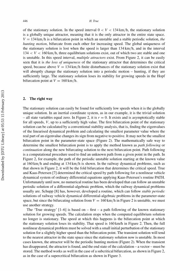
of the stationary solution. In the speed interval 0 < V < 134 km/h, the stationary solutionis a globally unique attractor, meaning that it is the only attractor in the entire state space.V = 134 km/h is a bifurcation point in which an unstable and a stable periodic solution, thehunting motion, bifurcate from each other for increasing speed. The global uniqueness ofthe stationary solution is lost when the speed is larger than 134 km/h, and in the interval134 < V < 160 km/h, three equilibrium solutions exist, out of which two are stable and oneis unstable. In this speed interval, multiple attractors exist. From Figure 2, it can be easilyseen that it is the loss of uniqueness of the stationary attractor that determines the criticalspeed, because above V = 134 km/h finite disturbances of the stationary solution exist thatwill abruptly change the stationary solution into a periodic motion – hunting, if they aresufficiently large. The stationary solution loses its stability for growing speeds in the Hopfbifurcation point at V = 160 km/h.

2. The right way

The stationary solution can easily be found for sufficiently low speeds when it is the globallyunique solution. In an inertial coordinate system, as in our example, it is the trivial solution– all state variables equal zero. In Figure 2, it is r = 0. It exists and is asymptotically stablefor all speeds, V , up to a sufficiently high value. The first bifurcation point of the stationarysolution can be calculated by a conventional stability analysis, that is, finding the eigenvaluesof the linearised dynamical problem and calculating the smallest parameter value where thereal part of an eigenvalue changes its sign from negative to positive. It may not be the smallestbifurcation point in the parameter-state space (Figure 2). The mathematically safe way todetermine the smallest bifurcation point is to apply the method known as path following orcontinuation along the new bifurcating solution to the next bifurcation point. Path followingis a computational procedure used to find an unknown path from a given point in the path. InFigure 2, for example, the path of the periodic unstable solution starting at the known valueat 160 km/h and ending at 134 km/h is shown. In the railway dynamical problems, such asthat shown in Figure 2, it will be the fold bifurcation that determines the critical speed. Trueand Kaas-Petersen [7] determined the critical speed by path following for a nonlinear vehicledynamical system of ordinary differential equations applying Kaas-Petersen’s routine PATH.Unfortunately until now, no numerical routine has been developed that can follow an unstableperiodic solution of a differential-algebraic problem, which the railway dynamical problemsusually are. Schupp [8] has, however, developed a routine, which can follow stable periodicsolutions of railway vehicle dynamical differential-algebraic problems in the parameter-statespace, but since the bifurcating solution from V = 160 km/h in Figure 2 is unstable, we mustuse another strategy.

The ‘True strategy’ [1–6] is based on – first – a path following of the known stationarysolution for growing speeds. The calculation stops when the computed equilibrium solutionno longer is stationary. The speed at which this happens is the bifurcation point at whichthe stationary solution loses its stability. That speed is 160 km/h in Figure 2. Then, the fullnonlinear dynamical problem must be solved with a small initial perturbation of the stationarysolution for a slightly higher speed than the bifurcation point. The transient solution will tendto the nearest attractor in the state space since the stationary solution now is unstable. In mostcases known, the attractor will be the periodic hunting motion (Figure 2). When the transienthas disappeared, the attractor is found, and the end state of the calculation – a vector – must bestored. The method works as well in the case of a subcritical bifurcation, as shown in Figure 2,as in the case of a supercritical bifurcation as shown in Figure 3.

Dow

nloa

ded

by [

DT

U L

ibra

ry]

at 0

5:53

15

Febr

uary

201

3

Vehicle System Dynamics 447

120 125 130 135 140 145 150 155 160−0.1

0

0.1

0.2

0.3

0.4

0.5

0.6

0.7

0.8

0.9

V (km/h)

r (c

m)

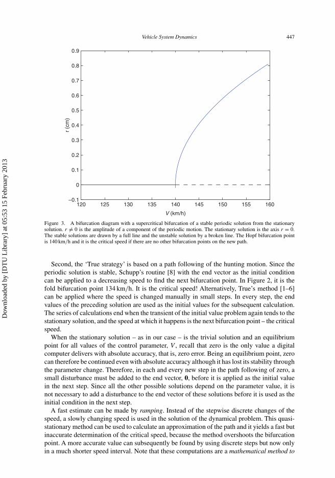
Figure 3. A bifurcation diagram with a supercritical bifurcation of a stable periodic solution from the stationarysolution. r �= 0 is the amplitude of a component of the periodic motion. The stationary solution is the axis r = 0.The stable solutions are drawn by a full line and the unstable solution by a broken line. The Hopf bifurcation pointis 140 km/h and it is the critical speed if there are no other bifurcation points on the new path.

Second, the ‘True strategy’ is based on a path following of the hunting motion. Since theperiodic solution is stable, Schupp’s routine [8] with the end vector as the initial conditioncan be applied to a decreasing speed to find the next bifurcation point. In Figure 2, it is thefold bifurcation point 134 km/h. It is the critical speed! Alternatively, True’s method [1–6]can be applied where the speed is changed manually in small steps. In every step, the endvalues of the preceding solution are used as the initial values for the subsequent calculation.The series of calculations end when the transient of the initial value problem again tends to thestationary solution, and the speed at which it happens is the next bifurcation point – the criticalspeed.

When the stationary solution – as in our case – is the trivial solution and an equilibriumpoint for all values of the control parameter, V , recall that zero is the only value a digitalcomputer delivers with absolute accuracy, that is, zero error. Being an equilibrium point, zerocan therefore be continued even with absolute accuracy although it has lost its stability throughthe parameter change. Therefore, in each and every new step in the path following of zero, asmall disturbance must be added to the end vector, 0, before it is applied as the initial valuein the next step. Since all the other possible solutions depend on the parameter value, it isnot necessary to add a disturbance to the end vector of these solutions before it is used as theinitial condition in the next step.

A fast estimate can be made by ramping. Instead of the stepwise discrete changes of thespeed, a slowly changing speed is used in the solution of the dynamical problem. This quasi-stationary method can be used to calculate an approximation of the path and it yields a fast butinaccurate determination of the critical speed, because the method overshoots the bifurcationpoint. A more accurate value can subsequently be found by using discrete steps but now onlyin a much shorter speed interval. Note that these computations are a mathematical method to

Dow

nloa

ded

by [

DT

U L

ibra

ry]

at 0

5:53

15

Febr

uary

201

3

448 H. True

find attractors – to solve an existence problem – which in principle has nothing in commonwith stability.

3. The wrong way

The application of a conventional stability analysis, that is, to find the eigenvalues of the lin-earised dynamical problem and calculate the smallest parameter value where the real part ofan eigenvalue changes its sign from negative to positive, is the wrong way to find the criticalspeed. The problem to be solved is not a stability problem, it is a problem of existence of solu-tions. A stability analysis will therefore in general not deliver the critical speed but only whatit can deliver: a stability limit for the stationary motion to infinitesimal initial disturbances! InFigure 3, the stability limit may indeed be the critical speed, but it is not so in Figure 2, whichillustrates the most often occurring case. It is never known in advance whether the bifurcationfrom the stationary solution is subcritical or supercritical. The difference between the bifurca-tion point on the stationary solution and the critical speed can be several hundred kilometresper hour for high-speed trains according to manufacturers! The details and the references areconfidential. Jensen [9] calculated in his PhD thesis the Hopf bifurcation point and the criticalspeed for a ‘half car’ of the Danish IC3 train, Figure 4. For an adhesion coefficient of 0.30,the critical speed is V = 317 km/h and the Hopf bifurcation point is 562 km/h.

It is necessary to follow the bifurcating periodic solution in order to find the smallestbifurcation point. Also in the case of a supercritical bifurcation – when the bifurcating periodicsolution is stable – it is necessary to follow the periodic solution to the next bifurcation point,because there may be a secondary bifurcation point in that branch from where a third solutionwill bifurcate to the left. This third solution might reach a smaller speed than the supercriticalbifurcation point found on the stationary solution.An example can be found in [10,11], where achaotic attractor bifurcates from the stable periodic solution and it disappears at a much lowerspeed in a so-called crisis. This speed is the critical speed. Another example was presented byGasch et al. [12].

Figure 4. The Hopf bifurcation point (upper curve) and the critical speed (lower curve) versus the coefficient ofadhesion for a ‘half car’ of the Danish IC3 train. The wheel profile is DSB 82-1 and the rails are UIC60 canted 1

40with the gauge 1435 mm.

Dow

nloa

ded

by [

DT

U L

ibra

ry]

at 0

5:53

15

Febr

uary

201

3

Vehicle System Dynamics 449

Figure 5. A one-dimensional nonlinear problem with three equilibrium points: the attractors −1 and 1, and 0, whichis unstable. The abscissa is the state space, and the ordinate, dy/dx, determines the direction of the flow on the x-axis.

Figure 6. A problem the same as that shown in Figure 5, the inclined line through −1 is the linearisation of thenonlinear dynamical problem around the point −1.

Dow

nloa

ded

by [

DT

U L

ibra

ry]

at 0

5:53

15

Febr

uary

201

3

450 H. True

Linearisations, such as those made in a conventional stability analysis of a nonlinear dynam-ical problem, must be treated with caution. First, we must choose an attractor in the nonlineardynamical problem that we can linearise around. In Figure 5, a simple one-dimensional exam-ple of a nonlinear dynamical problem is illustrated. In this problem, we choose the attractorx = −1. Then, we linearise the problem around x = −1 and find the linearisation (Figure 6).Then, we isolate the problem linearised around x = −1, see Figure 7, and find that the lin-earised problem only has one attractor, namely x = −1, and all other equilibrium points havedisappeared from the state space, which is the x-axis. Similarly, the vehicle dynamical problemthat is linearised around the bifurcation point on the stationary solution contains no informa-tion about other equilibrium solutions in Figure 2 and, in particular, none about the existenceof the hunting motion.

Linearisations are not always permitted. The first derivative of the function to be linearisedmust exist in the point of linearisation. For

√x, it does not exist in x = 0. The railway dynamical

problems are – practically all – non-smooth, and in the points of non-smoothness, the firstderivative of the force and torque functions is not defined. The Jacobian is needed when implicitroutines are applied for the numerical solution, but the Jacobian does not exist in the pointsof non-smoothness. Problems may also occur with the application of solvers of higher ordersto problems with a discontinuity of the second derivatives, which occur in the description ofa rail surface. The numerical procedure must therefore be modified in order to obtain reliableresults. Appropriate modifications can be found in the works by Xia [13] and Hoffmann [14],and True has discussed the modification in [2].

Figure 7. The problem shown in Figure 5 linearised around −1. Two of the equilibrium points have disappearedand with them every information about the stable equilibrium 1. When only the linearised problem is analysed is itimpossible to find the point 1.

Dow

nloa

ded

by [

DT

U L

ibra

ry]

at 0

5:53

15

Febr

uary

201

3

Vehicle System Dynamics 451

Two very recent papers on the numerical solution of vehicle dynamical problems are thestate-of-the-art paper by Arnold et al. [15] and the survey paper by True et al. [16].

4. Gambling

Some railway dynamicists feel that ‘the right method’for the calculation of the critical speed iseither too complicated or too slow. They therefore present and argue for modifications of ‘theright method’. Stichel [17] proposes the use of a finite disturbance of the stationary motion forgrowing speeds to find the periodic attractor. When it is found, the periodic attractor is followedbackwards for a decreasing speed – using ramping – until the hunting motion stops. Thereby,Stichel saves computer time for the path following of the stationary solution up to the Hopfbifurcation (which is very fast) and back again from there along the periodic attractor to thespeed at which he found the periodic attractor. This step can be time consuming. This methodis also ‘right’, because Stichel follows the hunting motion for a decreasing speed. Stichel’smethod is not a stability investigation. He conducts a legitimate search for other attractors inthe state space. Other authors, however, make the mistake of not following the hunting motionbackwards in the parameter-state space and call the speed at which the hunting motion firstoccurs, when the speed is increased, the critical speed. It is pure luck if the found speed isanywhere near the critical speed of the vehicle, because the found value of the speed dependson the size and the kind of the initial disturbance – an initial condition, which is only one ofthe many states that are excited in a real situation on the railway line. This method is thereforea gamble. By disturbing only one component of the initial value vector, valuable computertime is wasted with excitation of all the other components until the transient disappears.

The railway dynamicists in the Southwest Jiaotong university in Chengdu have alreadyrealised this. They use the data from the measurements of a sufficiently long section of arailway line as the input to the dynamical problem. In that case, several components of thestate of the vehicle are excited, and the critical speed found by growing speed will be basedon a seemingly realistic calculation. The found hunting motion was, however, not followedbackwards in the parameter-state space. During a visit to Chengdu in 2009, the author hadthe opportunity of testing the result of such a calculation together with one of its scientists.We started ramping, using commercial software, at the critical speed found by gambling in anearlier work. The hunting motion was now followed for a decreasing speed, but the calculationswere stopped when the speed had decreased by 10%, and the vehicle model was still hunting!Obviously, the critical speed in the model was lower than the one that had been claimed tobe the critical speed in the original report. In the test, a commercial routine was used, and itbecame obvious why ‘the right way’ is found cumbersome by dynamicists. The routine doesnot allow the download and storage of the end vector for a direct use as an initial value in thesubsequent calculation. This is, however, a shortage of the routine and not of the method. Onan earlier occasion, the author had the opportunity of using the same routine together with thehead of the IT department in Bombardier. He was able to modify the routine in less than halfan hour and enable its use in ‘the right method’. The calculations with ‘the right method’ thenran fast and without any problems.

The conclusion is that the published critical speeds that have been found by gambling arenot reliable – with the exception of Stichel’s work [17], because he actually completed hiscalculations in ‘the right way’.

It must be emphasised that the use of ‘the right method’ will not yield the correct resultin all theoretically possible cases. The author has, however, never found any of these ‘otherpossible cases’ during 25 years of railway dynamical research.

Dow

nloa

ded

by [

DT

U L

ibra

ry]

at 0

5:53

15

Febr

uary

201

3

452 H. True

5. The robustness of the hunting motion

More emphasis is often put on figures such as Figure 2 than what they are worth. For example,it is often stated – if we use Figure 2 as an example – that a lateral disturbance of the leadingwheel set �r > 0.2 cm at V = 157 km/h will initiate a hunting motion, and if �r < 0.2 cm,then the transient will die out. It is tacitly assumed that the point (157, 0.2) lies on the unstablelimit cycle and that it separates the domain of attraction of the stationary motion, which is anattractor, from the domain of attraction of the hunting motion, which is also an attractor. Thestatement is wrong, because the state space is multi-dimensional, and it is only in the one-dimensional state space that a point can separate two domains of attraction. As an example,see the unstable point 0 in Figure 5. Furthermore, it is impossible to determine the positionof the unstable limit cycle of differential-algebraic problems numerically in the state spaceby the methods available today. Daniele Bigoni, one of the students of the author, has evendemonstrated that a disturbance of only the lateral motion of the leading axle, a little bit largerthan the amplitude of the stable limit cycle, may start a transient that tends asymptoticallyto the stationary motion. This is certainly possible in a multi-dimensional state space. Moredetails are given in the next section on multi-dimensional spaces.

A simple two-dimensional example will illustrate the point made. Consider Figure 8 withan unstable limit cycle – the ellipse – in a state space with the lateral displacement of theleading wheel set as the abscissa and the yaw angle as the ordinate. The point (0, 0) is anattractor, and the interior of the ellipse is the domain of attraction of (0, 0). The exterior ofthe ellipse is the domain of attraction of another attractor further away. The point (157, 0.2) inFigure 2 corresponds to one of the points (±0.2, 0) in Figure 8, and it can be easily seen that foryaw = 0, all the trajectories through the points |x| < 0.2 will approach (0, 0), because theylie in the domain of attraction of that point.

−0.2 −0.15 −0.1 −0.05 0 0.05 0.1 0.15 0.2−0.08

−0.06

−0.04

−0.02

0

0.02

0.04

0.06

0.08

Lateral displacement, (cm)

Yaw

ang

le, (

°)

Figure 8. A stable equilibrium point (0, 0) surrounded by an unstable limit cycle. The interior of the limit cycle isthe domain of attraction of (0, 0). The exterior of the limit cycle is the domain of attraction of another attractor furtheraway.

Dow

nloa

ded

by [

DT

U L

ibra

ry]

at 0

5:53

15

Febr

uary

201

3

Vehicle System Dynamics 453

If, on the other hand, the yaw �= 0, then there are points with abscissae |x| < 0.2 – forexample, also x = 0 – through which the transients will run away from (0, 0), because thepoints lie outside the domain of attraction of (0, 0). So, it is possible in Figure 2 – where �ris the only component of the state of the system – that the disturbance of another mode canstart hunting of the vehicle even for �r = 0.

The conclusion is that the existence of an unstable limit cycle should not be indicated bya curve on the bifurcation diagrams of dynamical systems in state spaces of dimension 2 orhigher because it may lead to misinterpretations.

We have seen that in railway vehicle dynamics there very often exists a speed interval inwhich multiple attractors exist – namely the stationary motion and the hunting motion. It isalso a fact that the hunting motion is more robust in the sense that it is easy to start hunting,but virtually impossible to stop hunting without slowing down the vehicle. Due to the greatcomplexity of the attractors in the high-dimensional state space, it is impossible to explainthis fact exactly, but a simple picture may make it plausible. In Figure 9, the small ellipse,which is an unstable limit cycle, splits the domains of attraction of the stable equilibrium point(0, 0), on the one side, and the domain of attraction of the stable limit cycle, the large ellipse,on the other side. The angle φ covers the domain of arguments of the vectors from P that canend inside the unstable limit cycle, the domain of attraction of the stable equilibrium point(0, 0). Here – in two dimensions – it is easily seen that a sufficiently large initial disturbanceof (0, 0) will start the hunting independently of its direction in the plane. In contrast, an initialdisturbance on the ‘hunting ellipse’ must not only be sufficiently large – and not too large –but also lie inside the angle φ in order to reach the domain of attraction of (0, 0). Furthermore,(0, 0) is an equilibrium point, that is, independent of time, while the point P moves around onthe large ellipse all the time, whereby φ changes place and size.

Figure 9. A picture of an unstable limit cycle – the small ellipse – with a stable equilibrium point in the centre,surrounded by a stable limit cycle – the large ellipse.

Dow

nloa

ded

by [

DT

U L

ibra

ry]

at 0

5:53

15

Febr

uary

201

3

454 H. True

6. Multi-dimensional state spaces

The unstable limit cycle will lie on a surface in the N-dimensional state space. It can be mathe-matically proven that close to the subcritical bifurcation point, this surface has a tangent planethat is spanned by the eigenvectors belonging to the complex conjugated purely imaginaryeigenvalues at the bifurcation point. The limit cycle is the base of the generators of an (N − 1)-dimensional cylindrical subspace, which is the inset of the unstable limit cycle. It divides theN-dimensional state space into a domain of attraction of the origin and a domain of attrac-tion of the stable limit cycle – the hunting motion. Without showing the actual geometry inthe N-dimensional state space, Figure 10 might help the reader to understand the underly-ing dynamics. The cylindrical surface shown in Figure 10 is generated by a projection of an(N − 1)-dimensional subspace onto a two-dimensional surface. All the trajectories on thiscylindrical surface drift towards the unstable limit cycle while at the same time swirlingaround on the cylindrical surface. Outside the cylindrical surface, all the trajectories approach

Figure 10. A pictorial presentation of the unstable limit cycle in a three-dimensional space. The interior of thecylinder is the domain of attraction of the trivial solution. The limit cycle is a saddle cycle, which is the boundary ofa surface on which all solutions spiral towards zero. Outside the cylinder, all solutions drift towards the stable limitcycle far away. The structure of the cylindrical surface in the N-dimensional space is given in the upper corner, whereeach of the coordinate planes again has a similar three-dimensional structure and each of these coordinate planesagain has a three-dimensional . . . and so on until the dimension N − 1 has been reached in the full state space.

Dow

nloa

ded

by [

DT

U L

ibra

ry]

at 0

5:53

15

Febr

uary

201

3

Vehicle System Dynamics 455

the stable limit cycle, and inside the surface, all the trajectories approach zero in a swirlingfashion. In a state space with dimension 3 or higher, it is the inset and NOT the unstable limitcycle that splits the state space into the two domains of attraction of, respectively, zero andthe hunting motion.

The tangent plane mentioned above lies obliquely in the state space with respect to someof the axes in the N-dimensional state space with projections of the limit cycle onto theseaxes of non-zero lengths. These axes represent the modes that are excited with the loss ofthe stability of the trivial solution in the subcritical bifurcation point. The tangent plane willbe perpendicular to the remaining axes. With a decreasing speed, the unstable limit cycle willbe deformed in such a way that its projections on all the axes in the N-dimensional state spacewill have a finite length, meaning that all modes of the dynamical system become excited.The shape of the deformed unstable limit cycle in the state space cannot be computed bythe methods available today. An example of a closed curve in a three-dimensional space isshown in Figure 11.

Three different examples indicate that the domain of attraction of the trivial solution in theN-dimensional state space winds around the stable limit cycle in such a way that a very largedisturbance may push the solution back onto the trivial one – but only for a short time. First,Jens Christian Jensen (personal communication) numerically demonstrated to the author in arealistic dynamical model of a bogie that a large disturbance may stop the hunting. Second,TTCI in Pueblo demonstrated to the author in a field test with a gondola wagon that the huntingmotion of the wagon at a certain speed would abruptly end when the wheel sets are hit hardat the point in a frog. A few seconds later, the hunting starts again as could be expected. The

Figure 11. A closed curve in a three-dimensional xyz-space. Its projections on all the three coordinate planes areclosed plane curves. The curve in the xz-plane is degenerate because the x- and z-components are in phase.

Dow

nloa

ded

by [

DT

U L

ibra

ry]

at 0

5:53

15

Febr

uary

201

3

456 H. True

Figure 12. A demonstration in a three-dimensional state space as to how a disturbance of a single mode with Vnear by but larger than the fold bifurcation (the critical speed) can lie in the domain of attraction of the trivial solution,although the size of the disturbance is larger than the coordinate of the amplitude of the stable limit cycle. r is theordinate shown in Figure 2. (1) is a part of the unstable limit cycle in the neighbourhood of its maximum value of rwith a part of its inset on a conically shaped surface below. The domain of attraction of the trivial solution lies to theleft of the surface. (2) is a part of the stable limit cycle (the hunting motion). a is the largest r-value of the unstablelimit cycle, b is the largest r-value of the stable limit cycle and c > b is the intersection of the r-axis with the insetof the unstable limit cycle.

test wagon had three-piece freight trucks, of which one had the snubbers removed, and it wasthis truck that would stop hunting by passing the point. Third, von Wagner [18] has calculatedthe domain of attraction of the trivial solution for a simple model of a wheel set. He showedsome projections of the domain onto coordinate planes, where the projection of the domainof attraction was not connected.

Let us again consider the case of multiple attractors. In Figure 10, we can see that thereexists an unstable limit cycle – a saddle cycle, which is the base of the inset – the subspace thatseparates the two domains of attraction of zero and the hunting motion, respectively. Figure 10illustrates the geometry of the state space at a speed smaller than but very close to the subcriticalbifurcation. The stable limit cycle is so far away that it cannot be seen in the figure. With adecreasing speed, the two limit cycles and the cylindrical surface are strongly deformed, andthe limit cycles approach each other. Figure 12 illustrates in 3D how the situation may looklocally, when the speed is larger than but close to the fold bifurcation point. The limit cyclesare deformed but close to each other, and the inset may locally have a shape that is conical. Wecan see that an initial value vector with one component r|b < r < c, and all other componentsequal to zero, can fall inside the domain of attraction of the stationary solution although r islarger than the projection, b, of the amplitude of the stable limit cycle on the r-axis.

7. Driving with supercritical speed and chaos

It is often written in technical articles that ‘driving with supercritical speed’ is dangerous.I would warn against the use of the word ‘dangerous’ because many – if not most – freightwagons hunt at the normal service speeds. The public might get the impression that the highly

Dow

nloa

ded

by [

DT

U L

ibra

ry]

at 0

5:53

15

Febr

uary

201

3

Vehicle System Dynamics 457

praised safety on the railways is not guaranteed. Hunting is certainly undesirable, but it isonly dangerous in extreme situations, for example, when the track or the vehicle has seriousdefects.

Self-excited chaotic oscillations were never found worse than hunting in any of the numericalinvestigations that the author and his co-workers have performed. The amplitudes of the chaoticmotion were of the same order of magnitude as those of the hunting – when the solutions inthe state space lie on chaotic attractors. The chaotic attractors attract the solutions in theirneighbourhood in the state space so strongly that the external excitations are bounded and dieout very fast.

In contrast, motions that are characterised as chaotic transients may be dangerous and mustbe avoided. The amplitudes of chaotic transients may be very large and in real life lead to dan-gerous situations. Chaotic transients may, for example, appear as a transient motion betweentwo competing attractors. They have been found by the author in numerical investigations oflow-dimensional dynamical systems such as the famous Lorenz system. At a certain parametercombination, a pair of stable equilibrium points exist in the Lorenz problem. Certain initialconditions can start a transient motion with large amplitudes. It has a chaotic nature, for exam-ple, sensitivity of the motion to infinitesimal changes of the initial conditions, and the motionmay prevail for a fair amount of time until it dies out in one of the equilibrium points. Pascal[19] has simulated the occurrence of a derailment of a chaotically moving freight wagon. Theamplitudes of the oscillations became so large that the wagon derailed. Due to the continuousexcitation from the track, the chaos must be characterised as ‘transient’, because the wagonnever reached an equilibrium state. The author recommends the book by Moon [20] for furtherstudies on chaos, but it is only one of many.

8. Comments on the determination of the critical speed of real railway vehicles inroad tests

This article has dealt with the theoretical aspects of defining and calculating the critical speedof vehicles. The method, however, carries over to the measurements of the critical speed in roadtests. The critical speed of a real railway vehicle must be determined by ‘Stichel’s method’.It is mandatory that the critical speed is measured as the speed at which the hunting stopsduring idle deceleration. The method has been used at least in Germany for decades. The testvehicle running idle is pushed by an accelerating motorised vehicle until the test vehicle beginshunting. Then, the motorised vehicle slows down to release the test vehicle, which then runsidle and slows down due to friction and air resistance. When the test vehicle stops hunting, thecritical speed is reached. The method used is the ramping method, which is described in thesection ‘The right way’. It is impossible to accelerate a railway vehicle on a real railway lineall the way up to the speed of the subcritical bifurcation, because the track irregularities onall tracks in normal service are so large that the vehicle during acceleration will hunt beforethe speed of the subcritical bifurcation point is reached. So, the proposed method correspondsto ‘Stichel’s method’ described in the section ‘Gambling’. It is fortunate that it is impossiblein the case with multiple attractors to reach the speed of the subcritical bifurcation, becauseit may be hundred or more kilometres per hour higher than the critical speed. In practice,therefore, the length of the track section needed for the idle slow down of the test vehicle isreasonable.

The results of an application of ‘the right method’ or ‘Stichel’s method’ do not depend onthe criteria chosen for the variable(s) that is/are calculated or measured. The physical lawsand mathematical theorems guarantee that the disturbed motion in real life will not lead to

Dow

nloa

ded

by [

DT

U L

ibra

ry]

at 0

5:53

15

Febr

uary

201

3

458 H. True

wrong results, because all the equilibrium solutions have a domain of attraction. The resultsare therefore independent of the imposed disturbances within a realistically applicable range.Therefore, the criteria can be expressed as limits for displacements, rotations, velocities oraccelerations of vehicle components. It is important to remember that it is not the amplitudeof a disturbance that defines the critical speed but the significant change of the amplitude,when the decelerating vehicle passes the critical speed. The amplitude of a hunting motion isnot well defined, but the decreasing speed, where the amplitude abruptly changes, is.

The standard of the selected railway line must, of course, be so high that it is possible todistinguish between the calculated or measured amplitudes caused by the deviations from theideal track geometry and those caused by the errors plus hunting. The critical speed in curvesmay be lower than the critical speed on the tangent track. The effect is only relevant for curveswith large radii, because the maximum speed in curves with radii below, say, 1000 m. usuallyis lower than the critical speed of the vehicle in these curves.

In the theoretical problem, the engineer can choose all the parameters in his vehicle/trackmodel at will, but that is not possible in practice. The coefficient of adhesion, which is animportant parameter in the wheel/rail stress relations, depends on the weather conditions andit may vary along the test track and with the time of the day. The suspension system in thereal vehicle is manufactured with tolerances, and last but not least, a suitable section of arailway line must be available for the test. All this gives rise to practical problems that mustbe solved before ‘Stichel’s method’ can be used in real-life tests for a reliable and repeatabledetermination of the critical speed of a railway vehicle.

9. Conclusion

The only safe computation of the theoretical critical speed of a railway vehicle uses the rightway described in the section ‘The right way’, possibly using the modification proposed byStichel [17] described in the section ‘Gambling’. All other results are unreliable. In road testsof real vehicles, the same method applies by letting the vehicle roll out idling and measure thespeed at which the hunting stops.

References

[1] H. True, On the theory of nonlinear dynamics and its applications in vehicle systems dynamics, Veh. Syst. Dyn.31 (1999), pp. 393–421.

[2] H. True, Dynamics of railway vehicles and rail/wheel contact, DynamicAnalysis ofVehicle Systems, TheoreticalFoundations and Advanced Applications, CISM Courses and Lectures – No. 497, Springer, Wien New York,2007, pp. 75–128. Available at http://www2.imm.dtu.dk/pubdb/p.php?5617.

[3] H. True, Does a critical speed for railroad vehicles exist? RTD-Vol. 7, Proceedings of the 1994 ASME/IEEEJoint Railroad Conference, Chicago, Ill, March 22–24, 1994, American Society of Mechanical Engineers, 1994.

[4] H. True, Nichtlineare Schienenfahrzeugdynamik, neue Grundlagen, Methoden und Ergebnisse, ZEVrail GlasersAnnalen 128 (2004), pp. 526–537.

[5] H. True, Recent advances in the fundamental understanding of railway vehicle dynamics, Int. J. Veh. Des.40 (2006), pp. 251–264.

[6] H. True, On the critical speed of high-speed railway vehicles, Workshop: Noise and Vibration on High-SpeedRailways, 2 and 3. October 2008, FEUP Porto, Portugal, Civil Engineering Department, Faculty of Engineeringof the University of Porto, 2008, pp. 149–166.

[7] H. True and Chr. Kaas-Petersen, A bifurcation analysis of nonlinear oscillations in railway vehicles, Proceedingsof the 8th IAVSD-IUTAM Symposium on Vehicle System Dynamics, The Dynamics of Vehicles on Roads andTracks, Swets & Zeitlinger, 1984, pp. 655–665.

[8] G. Schupp, Computational bifurcation analysis of mechanical systems with applications to railway vehicles,Proceedings of the 18th IAVSD Symposium on Vehicle System Dynamics, The Dynamics of Vehicles on Roadsand on Tracks, Taylor & Francis, 2004, pp. 458–467.

Dow

nloa

ded

by [

DT

U L

ibra

ry]

at 0

5:53

15

Febr

uary

201

3

Vehicle System Dynamics 459

[9] J.C. Jensen, Teoretiske og Eksperimentelle Undersøgelser af Jernbanekøretøjer (in Danish), Ph.D. thesis, IMM,The Technical University of Denmark, 1995.

[10] F. Xia and H. True, On the dynamics of the three-piece-freight truck, RTD-Vol. 25, IEEE/ASME Joint RailConference, Chicago Ill., 22–24 April 2003, American Society of Mechanical Engineers, 2003, pp. 149–159.

[11] F. Xia and H. True, The dynamics of the three-piece-freight truck, Proc. 18th IAVSD Symposium on VehicleSystem Dynamics, The Dynamics of Vehicles on Roads and on Tracks, Taylor & Francis, 2004, pp. 212–221.

[12] R. Gasch, D. Moelle, and K. Knothe, The effects of nonlinearities on the limit-cycles of railway vehicles,Proceedings of the 8th IAVSD IUTAM Symposium on Vehicle System Dynamics, The Dynamics of Vehicleson Roads and Tracks, Swets & Zeitlinger, 1984, pp. 655–665.

[13] F. Xia, The dynamics of the three-piece-freight truck, Ph.D. thesis, IMM, The Technical University of Denmark,2002.Available at http://www2.imm.dtu.dk/pubdb/public/search.php?searchstr=Fujie+Xia &n=5&searchtype=strict.

[14] M. Hoffmann, Dynamics of European two-axle freight wagons, PhD. thesis, IMM, The Technical University ofDenmark, 2006. Available at http://www2.imm.dtu.dk/pubdb/views/publication_details.php?id=4853.

[15] M. Arnold, B. Burgermeister, C. Führer, G. Hippmann, and G. Rill, Numerical methods in vehicle systemdynamics: State of the art and current developments, Veh. Syst. Dyn. 49 (2011), pp. 1159–1207.

[16] H. True, A.P. Engsig-Karup, and D. Bigoni, On the numerical and computational aspects of non-smoothnessesthat occur in railway vehicle dynamics, Math. Comput. Simulation, (2012), http://dx.doi.org/10.1016/j.matcom.2012.09.016.

[17] S. Stichel, Modellierung und Parameterstudien zum Fahrverhalten von Güterwagen mit UIC-Fahrwerken, ZEVGlasers Annalen 23 (1999), pp. 289–296.

[18] U. von Wagner, Nonlinear dynamic behaviour of a railway wheelset, Veh. Syst. Dyn. 47 (2009), pp. 627–640.[19] J.-P. Pascal, Oscillations and chaotic behaviour of unstable railway wagons over large distances, Chaos Solitons

Fractals 5 (1995), pp. 1725–1753.[20] F.C. Moon, Chaotic and Fractal Dynamics, John Wiley & Sons, New York, 1992.

Dow

nloa

ded

by [

DT

U L

ibra

ry]

at 0

5:53

15

Febr

uary

201

3